Embed Size (px)
Citation preview
The Pennsylvania State University
The Graduate School
Energy & Geo-Environmental Engineering
HIGH TEMPERATURE CONDUCTIVITY PROBE FOR MONITORING
CONTAMINATION LEVELS IN POWER PLANT BOILER WATER
A Thesis in
Energy & Geo-Environmental Engineering
by
Sarah Hipple
2008 Sarah Hipple
Submitted in Partial Fulfillment of the Requirements
for the Degree of
Master of Science
August 2008

The thesis of Sarah Hipple was reviewed and approved* by the following:
Serguei Lvov Professor of Energy & Mineral Engineering Professor of Materials Science & Engineering Thesis Advisor
Jeffrey Brownson Assistant Professor of Energy & Mineral Engineering
Derek Elsworth Professor of Energy & Mineral Engineering
Jonathan Mathews Assistant Professor of Energy & Mineral Engineering Graduate Program Chair of Energy & Mineral Engineering
*Signatures are on file in the Graduate School
iii
ABSTRACT
A high temperature/high pressure flow through probe was designed to measure
high temperature electrical conductivity of aqueous (aq) dilute electrolyte solutions, an
application which can be useful in determining the levels of impurities in power plant
boiler water. The experimental solutions were pure water, ammonia solution known as
the All Volatile Treatment (AVT regime) corresponding to 10-5 mol kg-1 NH4OH, and a
series of dilute NaCl solutions in the AVT regime. A series of probe designs resulted in
the use of two probes for two different systems. In the first system, a probe with
platinum black electrodes was tested in the temperature range of 25-350°C and at a
pressure of 18 MPa. The flow rate was constant at 6 cm3min-1. Contamination was a
problem with this system, so the second system and second probe were chosen to
eliminate some of the factors that contributed to the ionic impurities in our test solution.
The second probe, with a steel working electrode and gold reference electrode, was tested
in a temperature range of 25-350°C and at pressures of 5-18 MPa. The flow rate was
constant at 5 cm3min-1. The conductivity results for both experimental setups were
obtained using electrochemical impedance spectroscopy (EIS) methods and were
compared with the calculated conductivities of aqueous NaCl and ammonia test solutions.
Theoretical conductivities were calculated using the conductivity model with three
components as it was developed and described by R.H. Wood and coworkers:
Hnedkovsky et al. (2005) and Sharygin et al. (2006; 2001; 2002). The second probe
proved successful in determining the in-situ presence of a number of concentrations of
NaCl, which corresponded to the level of Cl- contamination in power plant boiler water.
iv
TABLE OF CONTENTS
LIST OF FIGURES .....................................................................................................v
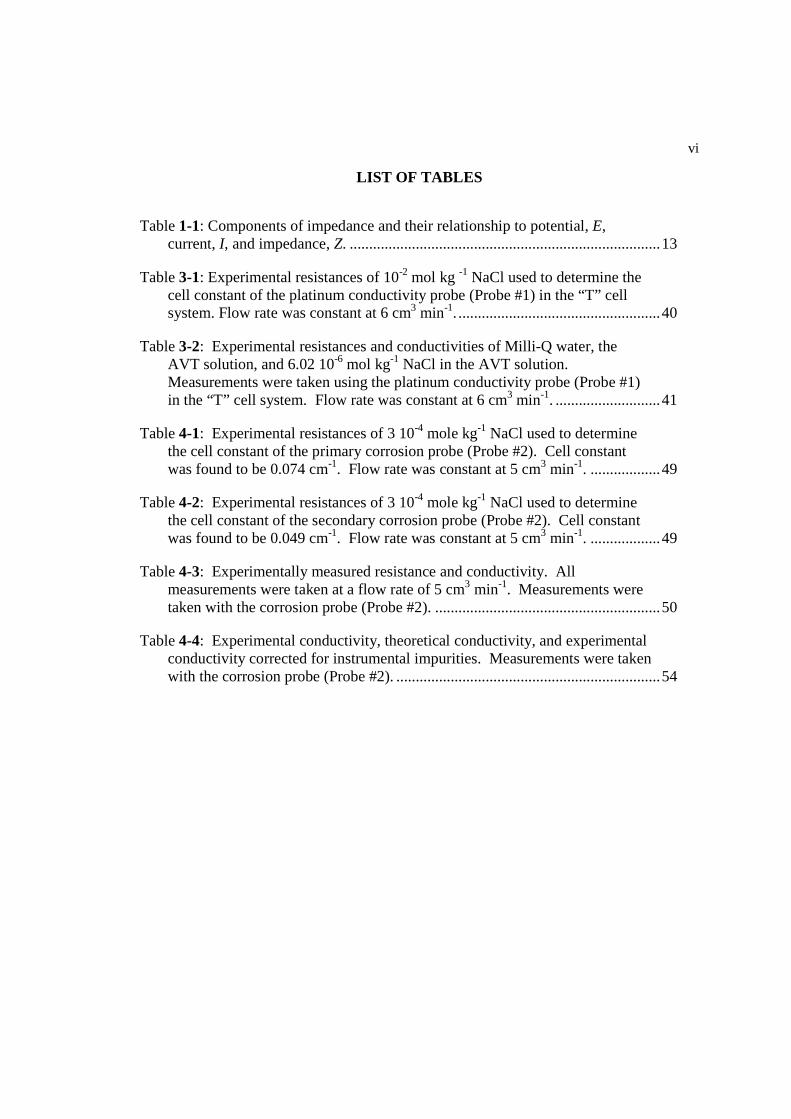
LIST OF TABLES.......................................................................................................vi
ACKNOWLEDGEMENTS.........................................................................................vii
Chapter 1 Introduction, Objectives, and Literature Review .......................................1
1.1 Basic Electrical Conductivity Theory.............................................................4 1.2 Experimental Electrochemical Impedance Spectroscopy (EIS) Methods ......12 1.3 Literature Review ...........................................................................................23 1.3.1 Previous high temperature conductivity measurements of NaCl (aq) ....23 1.3.2 Modern conductivity measurements of NaCl (aq)..................................23 1.3.3 Theoretical analysis of conductivity data ...............................................25 1.3.4 Instruments for in situ conductivity measurements of high
temperature/high pressure aqueous solutions................................................26
Chapter 2 Experimental Techniques...........................................................................29
2.1 Preparation of Solutions .................................................................................30 2.2 Conductivity Measurements ...........................................................................31
Chapter 3 First Experimental System .........................................................................35
3.1 Probe Design and Experimental Setup for First Experimental System..........35 3.2 Observed Data for First Experimental System ...............................................39
Chapter 4 Second Experimental System.....................................................................45
4.1 Probe Design and Experimental Setup for Second Experimental System .....45 4.2 Observed Data for Second Experimental System...........................................47
Chapter 5 Discussion, Conclusions, and Future Work...............................................57
5.1 Discussion of Experimental Procedure...........................................................57 5.2 Conclusions on the Applications of This Experimental Work .......................58 5.3 Recommendations for Future Work ...............................................................60
References....................................................................................................................62
v
LIST OF FIGURES
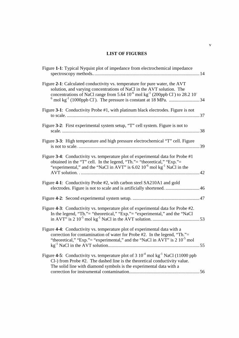
Figure 1-1: Typical Nyquist plot of impedance from electrochemical impedance spectroscopy methods.. .........................................................................................14
Figure 2-1: Calculated conductivity vs. temperature for pure water, the AVT solution, and varying concentrations of NaCl in the AVT solution. The concentrations of NaCl range from 5.64 10-6 mol kg-1 (200ppb Cl-) to 28.2 10-6 mol kg-1 (1000ppb Cl-). The pressure is constant at 18 MPa. ..........................34
Figure 3-1: Conductivity Probe #1, with platinum black electrodes. Figure is not to scale. .................................................................................................................37
Figure 3-2: First experimental system setup, “T” cell system. Figure is not to scale. .....................................................................................................................38
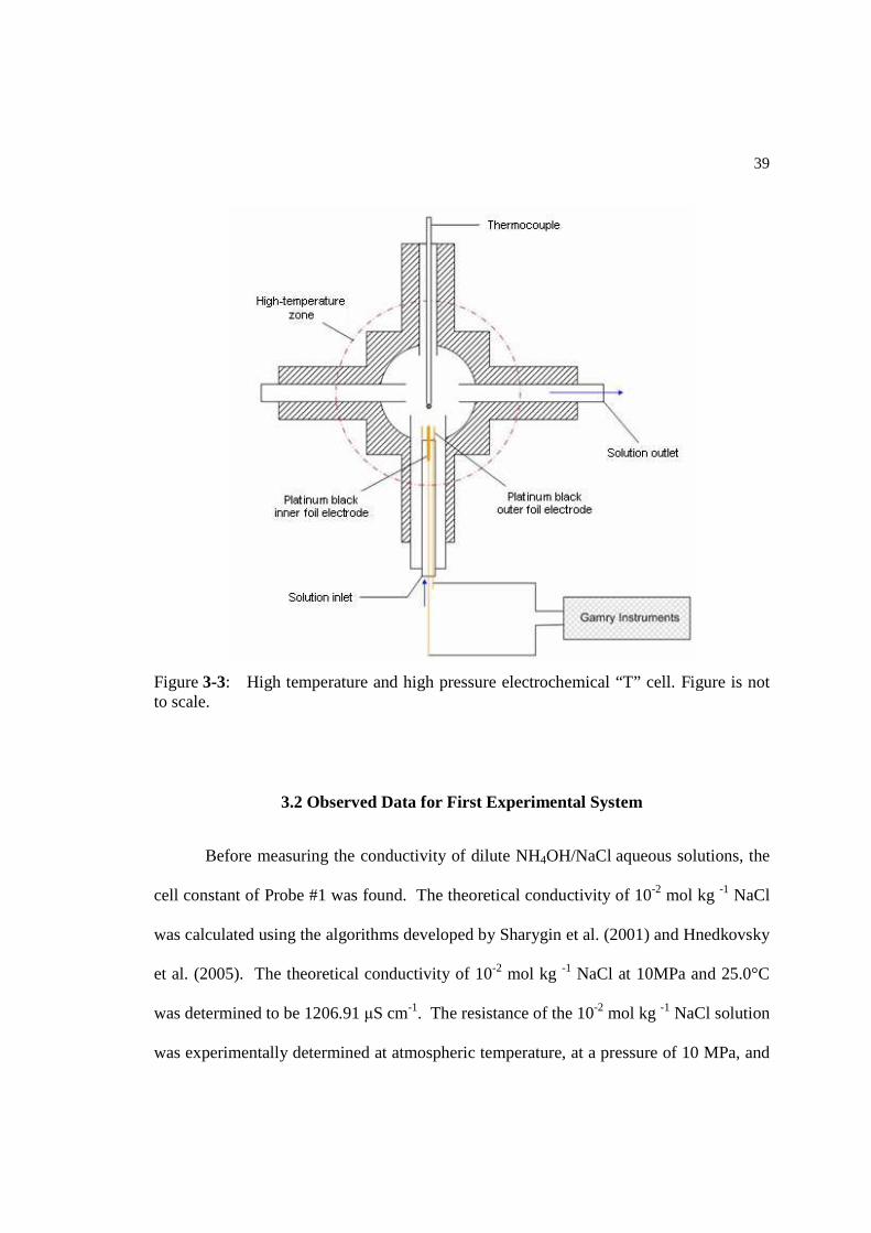
Figure 3-3: High temperature and high pressure electrochemical “T” cell. Figure is not to scale. .......................................................................................................39
Figure 3-4: Conductivity vs. temperature plot of experimental data for Probe #1 obtained in the “T” cell. In the legend, “Th.”= “theoretical,” “Exp.”= “experimental,” and the “NaCl in AVT” is 6.02 10-6 mol kg-1 NaCl in the AVT solution. . .....................................................................................................42
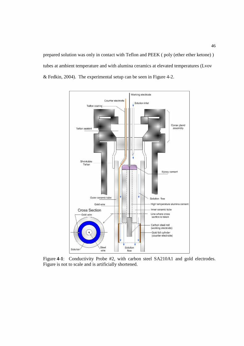
Figure 4-1: Conductivity Probe #2, with carbon steel SA210A1 and gold electrodes. Figure is not to scale and is artificially shortened. .............................46
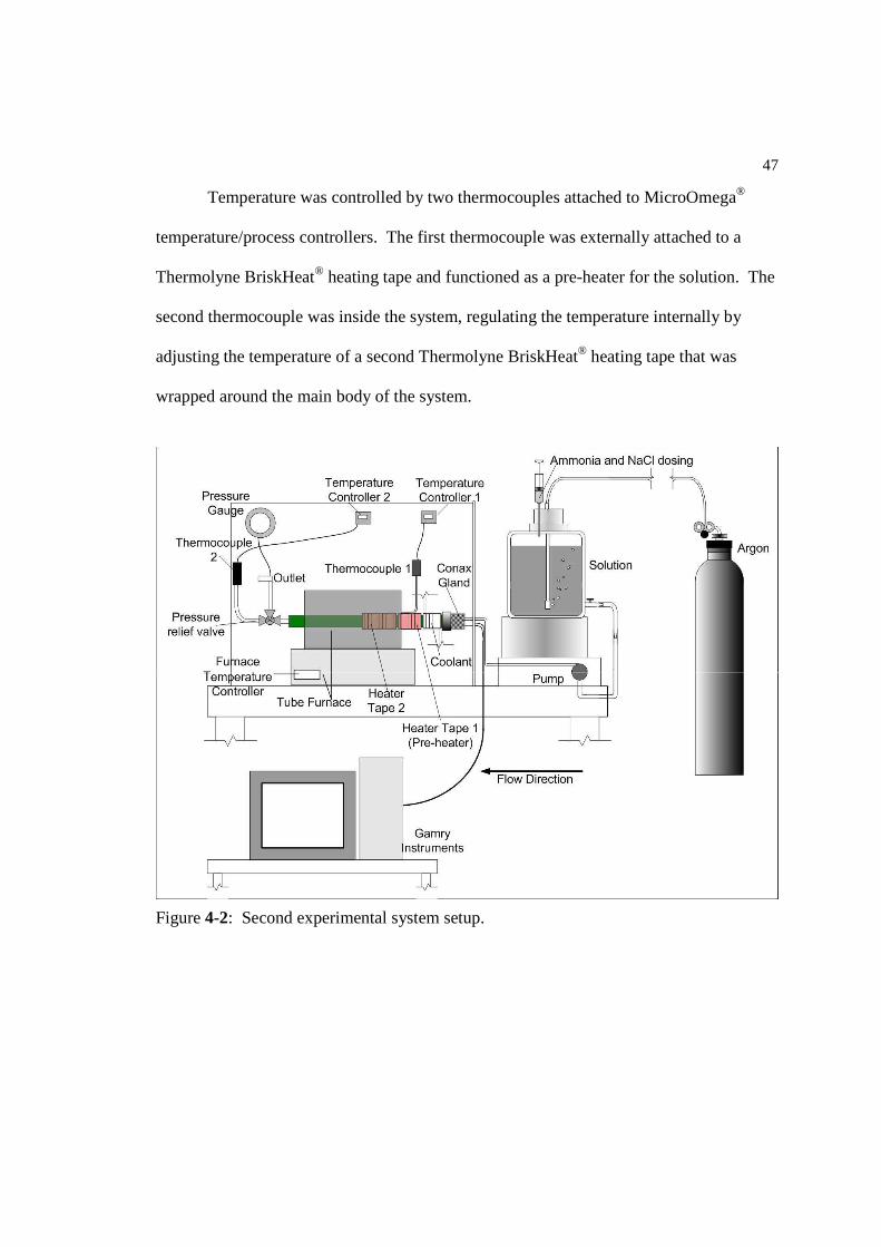
Figure 4-2: Second experimental system setup. .........................................................47
Figure 4-3: Conductivity vs. temperature plot of experimental data for Probe #2. In the legend, “Th.”= “theoretical,” “Exp.”= “experimental,” and the “NaCl in AVT” is 2 10-5 mol kg-1 NaCl in the AVT solution. ........................................53
Figure 4-4: Conductivity vs. temperature plot of experimental data with a correction for contamination of water for Probe #2. In the legend, “Th.”= “theoretical,” “Exp.”= “experimental,” and the “NaCl in AVT” is 2 10-5 mol kg-1 NaCl in the AVT solution..............................................................................55
Figure 4-5: Conductivity vs. temperature plot of 3 10-4 mol kg-1 NaCl (11000 ppb Cl-) from Probe #2. The dashed line is the theoretical conductivity value. The solid line with diamond symbols is the experimental data with a correction for instrumental contamination............................................................56
vi
LIST OF TABLES
Table 1-1: Components of impedance and their relationship to potential, E, current, I, and impedance, Z. ................................................................................13
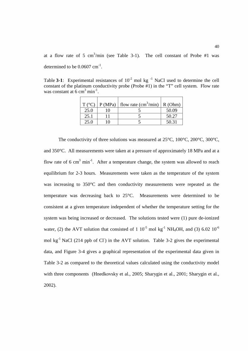
Table 3-1: Experimental resistances of 10-2 mol kg -1 NaCl used to determine the cell constant of the platinum conductivity probe (Probe #1) in the “T” cell system. Flow rate was constant at 6 cm3 min-1. ....................................................40
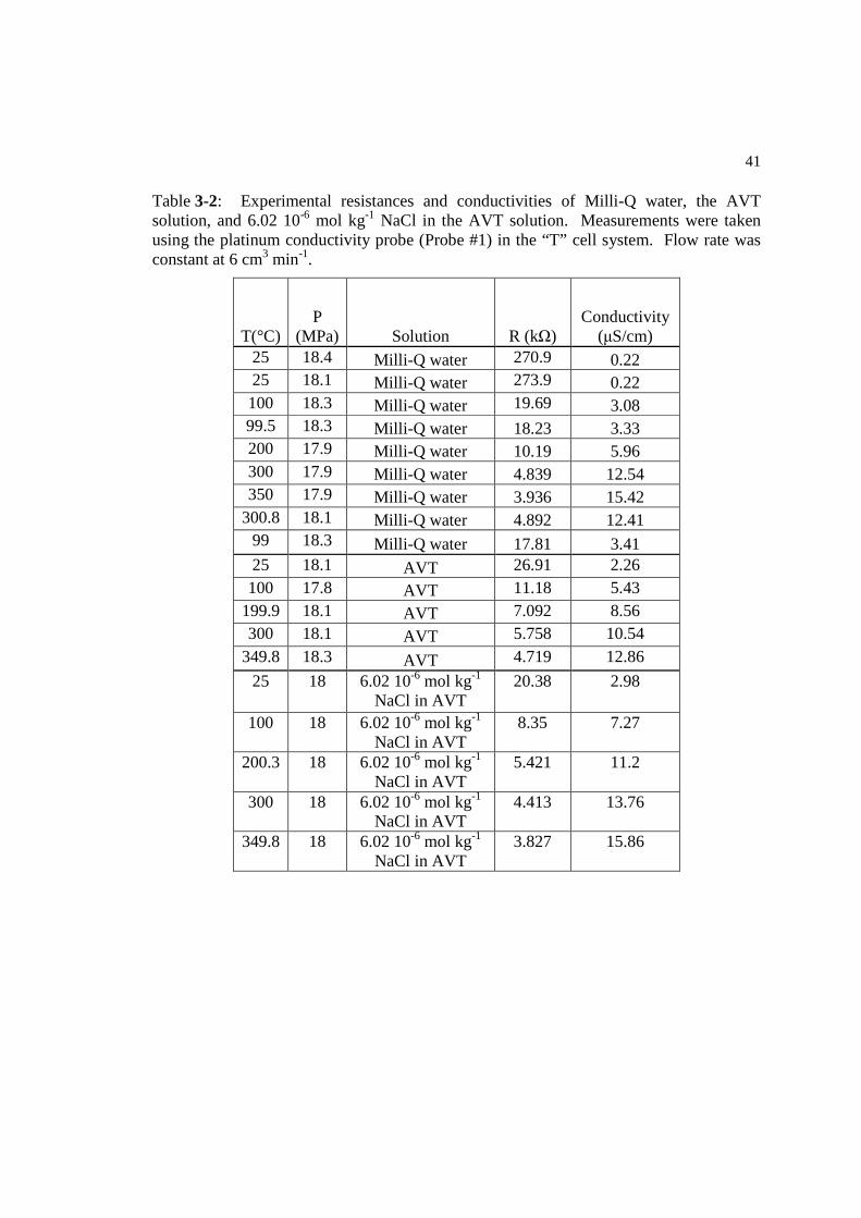
Table 3-2: Experimental resistances and conductivities of Milli-Q water, the AVT solution, and 6.02 10-6 mol kg-1 NaCl in the AVT solution. Measurements were taken using the platinum conductivity probe (Probe #1) in the “T” cell system. Flow rate was constant at 6 cm3 min-1. ...........................41
Table 4-1: Experimental resistances of 3 10-4 mole kg-1 NaCl used to determine the cell constant of the primary corrosion probe (Probe #2). Cell constant was found to be 0.074 cm-1. Flow rate was constant at 5 cm3 min-1. ..................49
Table 4-2: Experimental resistances of 3 10-4 mole kg-1 NaCl used to determine the cell constant of the secondary corrosion probe (Probe #2). Cell constant was found to be 0.049 cm-1. Flow rate was constant at 5 cm3 min-1. ..................49
Table 4-3: Experimentally measured resistance and conductivity. All measurements were taken at a flow rate of 5 cm3 min-1. Measurements were taken with the corrosion probe (Probe #2). ..........................................................50
Table 4-4: Experimental conductivity, theoretical conductivity, and experimental conductivity corrected for instrumental impurities. Measurements were taken with the corrosion probe (Probe #2). ....................................................................54
vii
ACKNOWLEDGEMENTS
I would like to acknowledge and thank my thesis advisor Dr. Serguei Lvov for
having given me the opportunity to conduct this research and for his confidence in my
abilities. Dr. Lvov was a key contributor to the research conducted for this thesis and an
editor of this thesis.
A great deal of thanks is owed to Dr. Victor Balashov for his advice and help
throughout the experimental and data treatment process. This project was inspired by his
work in the laboratory of Dr. Robert Wood at the University of Delaware. I would also
like to acknowledge Dr. Balashov as an editor of this thesis and as the creator of Figure
2-1, which was slightly modified by the author of this thesis for clarity.
I would like to thank the Electric Power Research Institute (EPRI) for funding the
research conducted for this thesis.
The help of Dr. Mark Fedkin was greatly appreciated, and I would like to
acknowledge him for his contributions to Figures 3-1, 3-3, and 4-1 within this thesis.
These images were created by Dr. Fedkin and modified by the author of this thesis to
depict the author’s experimental system.
The comments and contributions of my thesis advisory committee members, Dr.
Jeffrey Brownson and Dr. Derek Elsworth, were appreciated in the effort toward this
master’s degree.
I would also like to thank Nigel Laracuente for looking over my thesis for any
blatant errors or minor grammatical infractions.
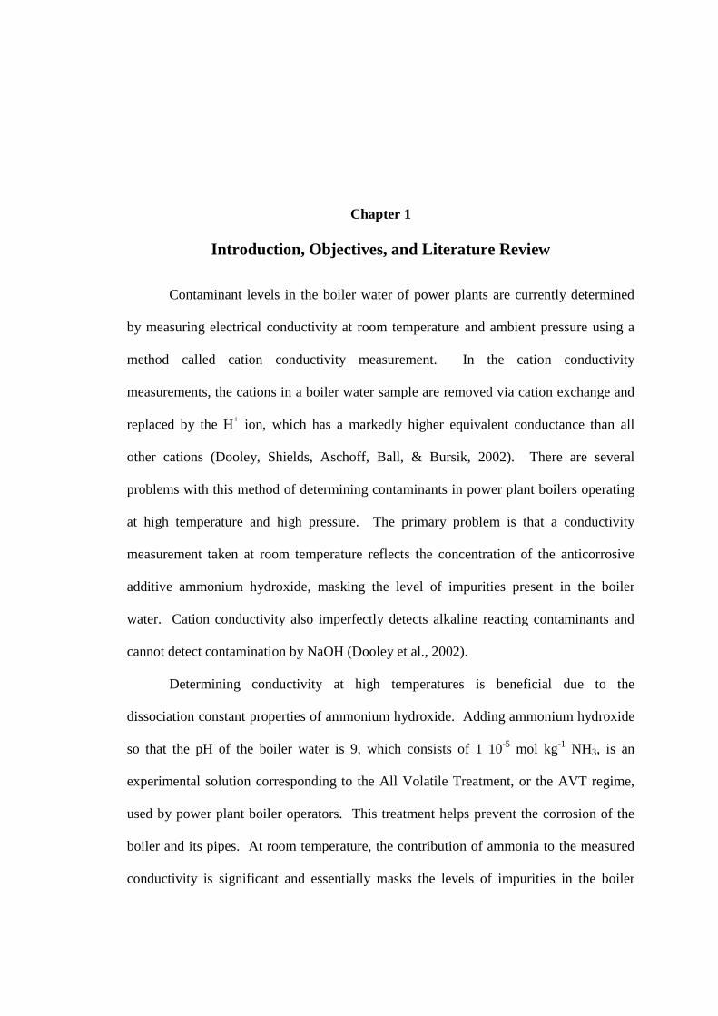
Chapter 1
Introduction, Objectives, and Literature Review
Contaminant levels in the boiler water of power plants are currently determined
by measuring electrical conductivity at room temperature and ambient pressure using a
method called cation conductivity measurement. In the cation conductivity
measurements, the cations in a boiler water sample are removed via cation exchange and
replaced by the H+ ion, which has a markedly higher equivalent conductance than all
other cations (Dooley, Shields, Aschoff, Ball, & Bursik, 2002). There are several
problems with this method of determining contaminants in power plant boilers operating
at high temperature and high pressure. The primary problem is that a conductivity
measurement taken at room temperature reflects the concentration of the anticorrosive
additive ammonium hydroxide, masking the level of impurities present in the boiler
water. Cation conductivity also imperfectly detects alkaline reacting contaminants and
cannot detect contamination by NaOH (Dooley et al., 2002).
Determining conductivity at high temperatures is beneficial due to the
dissociation constant properties of ammonium hydroxide. Adding ammonium hydroxide
so that the pH of the boiler water is 9, which consists of 1 10-5 mol kg-1 NH3, is an
experimental solution corresponding to the All Volatile Treatment, or the AVT regime,
used by power plant boiler operators. This treatment helps prevent the corrosion of the
boiler and its pipes. At room temperature, the contribution of ammonia to the measured
conductivity is significant and essentially masks the levels of impurities in the boiler
2
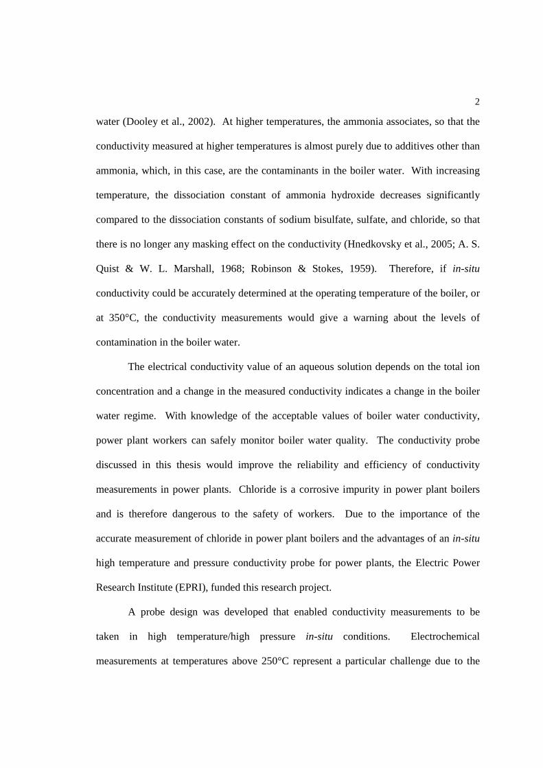
water (Dooley et al., 2002). At higher temperatures, the ammonia associates, so that the
conductivity measured at higher temperatures is almost purely due to additives other than
ammonia, which, in this case, are the contaminants in the boiler water. With increasing
temperature, the dissociation constant of ammonia hydroxide decreases significantly
compared to the dissociation constants of sodium bisulfate, sulfate, and chloride, so that
there is no longer any masking effect on the conductivity (Hnedkovsky et al., 2005; A. S.
Quist & W. L. Marshall, 1968; Robinson & Stokes, 1959). Therefore, if in-situ
conductivity could be accurately determined at the operating temperature of the boiler, or
at 350°C, the conductivity measurements would give a warning about the levels of
contamination in the boiler water.
The electrical conductivity value of an aqueous solution depends on the total ion
concentration and a change in the measured conductivity indicates a change in the boiler
water regime. With knowledge of the acceptable values of boiler water conductivity,
power plant workers can safely monitor boiler water quality. The conductivity probe
discussed in this thesis would improve the reliability and efficiency of conductivity
measurements in power plants. Chloride is a corrosive impurity in power plant boilers
and is therefore dangerous to the safety of workers. Due to the importance of the
accurate measurement of chloride in power plant boilers and the advantages of an in-situ
high temperature and pressure conductivity probe for power plants, the Electric Power
Research Institute (EPRI), funded this research project.
A probe design was developed that enabled conductivity measurements to be
taken in high temperature/high pressure in-situ conditions. Electrochemical
measurements at temperatures above 250°C represent a particular challenge due to the
3
limitations of material stability in sub- and super-critical hydrothermal environments
(Balashov, Fedkin, Lvov, & Dooley, 2007). This is the upper boundary for the stability
of Teflon®, and no other inert isolating polymeric material is available for use in high
temperature electrochemical systems, so a strategic cooling system was a necessary part
of the system design process (Balashov et al., 2007).
The purpose of this probe development was to develop a sensor that could
determine the level of contaminants in power plant boiler water by measuring
conductivity under in situ conditions. Power plant boiler water typically has low
concentrations of ionic species, so very dilute solutions were studied (Balashov et al.,
2007). For the dilute solutions, a flow through apparatus is necessary to accurately
measure conductivity, which is why a static cell design was not considered (Zimmerman,
Gruszkiewicz, & Wood, 1995).
This Laboratory had previously undertaken investigations into the most successful
electrode assembly design with controlled hydrodynamics that can be used for high
temperature and pressure conditions. It was determined that the fairly simple annular
duct geometry design was preferable to other possible designs, such as the wall-tube
geometry (Balashov et al., 2007).
1.1 Basic Electrical Conductivity Theory
Studying the conductivity of electrolytic solutions requires investigating the
ability of the ions in a solution to pass electrical current between two electrodes. The
following is an introduction to basic electrochemical conductivity theory. Several
4
interrelated terms such as conductivity, molar conductivity, conductance, and limiting
ionic conductivity are used in this thesis. The following section explains the relationship
between such terms and the properties that each term describes. The terms defined in this
section lay the groundwork for understanding the experimental methods used to measure
the conductivity of test solutions. These basic concepts are also important in
understanding the series of equations that were used to calculate the theoretical
conductivity of a solution.
In an electric field with strength E, ions with charge ze0 will be subject to
frictional force KR. The ion charge is from one unit of elementary charge, e0 with
e0=1.602 10-19 Coulombs and z is the charge number of the ion. Due to the frictional
force, which increases with any increase in the electric field strength, balancing E, ions
attain a terminal velocity, vmax. For a spherical ion with radius rI in a medium with
viscosity η (Hamann, Hamnett, & Vielstich, 1998),
Therefore, for a given viscosity and electric field strength, the transport velocity depends
upon the charge and radius of the solvated ion, and the sign of the ion determines its
direction of migration (Hamann et al., 1998).
The velocity of an ion, vmax, is a vector quantity that is dependent upon the
magnitude of the electric field E. When the geometry of the system is fixed, the
velocity is dependent upon the potential difference, ∆V, between electrodes. A scalar
value related to vmax but independent of the magnitude of the electric field is the mobility,
u, with units of m2 V-1 s-1, where (Hamann et al., 1998):
Ir
zev
πη60
max
E= (1.1)
5
The ionic mobility, ui, of an ion i is related to the diffusion coefficient, Di, of ion i
by the relationship Di = uikBT where kB is the Boltzmann’s constant and T is temperature
(Hamann et al., 1998).
The current measured between the electrodes can be given as the current per unit
area, I, and is related to mobility by the following equation (Hamann et al., 1998):
where A is the area of the electrode surface normal to the direction of flow, n+ is the
number of ions of unit charge z+ per unit volume and n- is similarly defined. If there are
more than two types of ion in the solution, the summation to determine current would
include all ions (Hamann et al., 1998).
If the geometry is fixed such that the distance between electrodes is l and the
potential difference between electrodes is ∆V, then E= ∆V/l, and we have (Hamann et
al., 1998):
with
where G is the conductance of the electrolyte solution with units of Ω-1 or siemens, S.
Ir
zevu
π60max ==
E (1.2)
E)(0−−−+++ += uznuznAeI (1.3)
VGI ∆= (1.4)
)(0−−−+++ += uznuzne
l
AG (1.5)
6
As can be seen, the conductance is dependent upon the geometry of the setup,
whereas the conductivity, κ, with units of Ω-1 m-1 or S m-1, is a characteristic property of
the electrolyte solution given by (Hamann et al., 1998):
where R is the solution resistance with units of Ω, which is equal to the inverse of
conductance, and ρ, with units of Ω m, is the intrinsic property of the solution known as
resistivity.
The conductivity of a solution is dependent upon its concentration. The above
equation defines κ with respect to concentration n, but in order to define conductivity
with respect to the more typical concentration c in units of mol m-3, consider the
electrolyte Aυ+Bυ- which dissociates into the ions Az+ and Bz-. From the principle of
electroneutrality, z+υ+=z-υ-≡z±υ±. Note that the term z±υ± is called the equivalent number
of the electrolyte. Now κ can be defined with respect to concentration c (Hamann et al.,
1998):
where L is Avagadro’s number and υ± is the number of cation or anion per formula unit
of electrolyte.
Once conductivity is defined with respect to the concentration of the electrolyte
solution, a term that separates concentration from mobility can be defined. The molar
conductivity, Λ, with units of Ω-1 mol-1 m2, and equivalent molar conductivity, Λeq, are
given by the following equations (Hamann et al., 1998):
)(1
0−−−+++ +==== uznuzne
RA
l
A
lG
ρκ (1.6)
)(0−+
±± += uucLezυκ (1.7)
7
Molar conductivity and equivalent molar conductivity are useful in studying the
relationship between concentration and mobility (Hamann et al., 1998).
The dependence between κ and c is nonlinear due to electrostatic interactions
between ions. This means that Λ is also dependent on concentration. To study
conductivity of an ion independent of interionic interactions, there must be no other ions
with which the ion of interest could interact. Therefore, the concept of molar
conductivity at infinite dilution, or limiting molar conductivity, Λ0, is studied. At low
concentrations of strong electrolytes there is a linear relationship between Λ and Λ0,
called Kohlrauch’s law (Hamann et al., 1998):
where c0 is a standard concentration, 1 mol dm-1, and k is a constant that is dependent
upon the electrolyte.
Since there are no ionic interactions at infinite dilution, the limiting ionic molar
conductivity, λ0, of each ion can be separately identified such that (Hamann et al., 1998):
where υ+/ υ- is the number of cation/anion per formula unit of electrolyte. For example,
for CuCl2, υ+= 1 and υ-=2. The above equation is also known as the law of independent
migration of ions, and this additive property of limiting ionic molar conductivities is
)(0−+
±± +==Λ uuLezc
υκ (1.8)
)(0−+
±±
+=Λ=Λ uuLezeq υ
(1.9)
00 c
ck−Λ=Λ (1.10)
−−
++ +=Λ 000 λνλν (1.11)
8
valuable in finding the limiting molar conductivity of weak electrolytes (Hamann et al.,
1998).
Strong electrolytes almost fully dissociate and therefore their conductivity is
dependent upon concentration as seen in Kohlrauch’s law. NaCl (aq) is an example of a
strong electrolyte. Kohlrauch’s law makes experimentation a valuable tool in
determining the limiting molar conductivity of strong electrolytes. For weak electrolytes,
such as ammonia, the variation of molar conductivity with concentration is dependent
upon the electrolyte’s degree of dissociation and a reaction’s dissociation constant. The
degree of dissociation is defined as the ratio of the amount of dissociated species to the
total amount of species present. The dissociation constant is the equilibrium constant for
a dissociation reaction and is a thermodynamic property directly related the Gibbs free
energy of the reaction. Due to the additive property of the law of independent migration
of ions, limiting ionic molar conductivities can be determined in strong electrolytes and
then be added to determine the limiting molar conductivities of weak electrolytes
(Hamann et al., 1998).
At infinite dilution, the ionic molar conductivities are independent of the
concentration of the electrolyte and are independent of the other ions in the solution. The
relationships above still hold true, but the mobilities and therefore the ionic molar
conductivities are not independent of each other or of the concentration in the following
relationships (Hamann et al., 1998).
since
−−−
+++
−−
++ +=+=Λ FuzFuz ννλνλν (1.12)
9
where F is Faraday’s constant with F= e0L.
The conductivity of an electrolyte solution is affected by several different effects
between ions. These effects determine the arrangement of ions within the solution.
Electrostatic forces cause like ions to repel and oppositely charged ions to attract, causing
a local ordering such that an ion is surrounded by a cloud of ions of an opposite charge
(Hamann et al., 1998).
Applying an electric field causes positive and negative ions to accelerate in
opposite directions, which distorts the local ordering such that the central ion is slightly
off center of its ionic cloud. Each ion attempts to re-center itself, and the time it takes to
do so is termed the relaxation time. Each central ion experiences drag due to the fact that
its ionic cloud is attempting to travel in the opposite direction of the central ion. This is
the relaxation effect and it increases with increased concentration (Hamann et al., 1998).
Another effect acting on ions in the solution is the electrophoretic effect. The
electrophoretic effect is when an individual ion experiences additional drag due to the
ionic cloud surrounding an oppositely charged ion. This effect depends on the viscosity
of the liquid and decreases the conductivity of a solution. The Debye-Hückel-Onsager
equation determines the molar conductivity of an electrolyte by taking into account the
relaxation effect and the electrophoretic effect and is given by the following equation.
The second term is a reduction in the conductivity due to the relaxation effect. The third
term accounts for the electrophoretic effect and depends upon the viscosity of the
solution (Hamann et al., 1998).
Fzu
+
++ = λ
(1.13)
10
where η is viscosity, ε0 is the absolute permittivity of free space with ε0 = 8.854 10-12 F
m-1, εr is the relative permittivity of a medium, and q and κd are given by the following
equations (Hamann et al., 1998):
where ci is the molarity or concentration in mol L-1, and c0 is the standard molarity with
c0 = 1 mol L-1. κd-1 is also known as the Debye screening length, and, at a distance
greater than approximately κd-1 from an ion, the ion’s electrostatic effect becomes very
small (Hamann et al., 1998).
When considering a fully dissociated 1-1 electrolyte, the Debye-Hückel-Onsager
equation can be reduced to Kohlrauch’s empirical law (Hamann et al., 1998).
As discussed above, an oppositely charged ion cloud surrounds an ion, and the
density of the ionic cloud increases with increased concentration. For an ion to be able to
react, energy must be input to remove the ionic cloud. The energy input is a loss for the
system and reduces the reactivity of the ion. Due to the greater density of the ionic cloud
in more concentrated systems, reactivity decreases with increased concentration. To
describe the thermodynamic or electrochemical properties of dissolved ions, a measure of
concentration, such as molality, does not account for the lost reactivity of an ion.
πηκκ
επε 6
)(
1
2
24
20
0
20
00dd
Br
zzLe
q
q
Tk
ezz −+−+ +−
+⋅Λ−Λ=Λ (1.14)
−++−
−+
−+
−+
++
⋅+
=00
00
λλλλzzzz
zzq
(1.15)
0
2
0
0202
c
cz
Tk
Lce iii
Brd
∑
=
εεκ (1.16)
11
Therefore, an effective molality, called activity, ai, for ion i is employed, with ai defined
as (Hamann et al., 1998):
where γi is the activity coefficient, which represents the deviation from ideality, mi is the
molality or concentration in mol kg-1, and m0 is the standard molality with m0=1 mol kg-1.
The only way to experimentally determine an activity coefficient is to determine
the mean activity coefficient of an electrolyte using the Debye-Hückel limiting law,
which is only applicable for very dilute solutions. The Debye-Hückel limiting law is
(Hamann et al., 1998):
where A is a constant that depends on the properties of the solvent, and, for water at
25°C, A=1.172. And I is the ionic strength, a unitless variable, given by (Hamann et al.,
1998):
At a given concentration, a solution’s conductivity is also affected by the relative
permittivity, or dielectric constant, of the medium. For an unvarying temperature, a
solvent’s dielectric constant is constant; however, the dielectric constant changes with
changes in temperature. The dielectric constant affects conductivity in the following
manner. The attraction between two species is governed by Coulomb’s Law. According
to Coulomb’s law, the energy of interaction between particles is inversely proportional to
0m
ma i
ii γ= (1.17)
I−+± −= zzAγ (1.18)
∑
=i
ii
m
mz
02
2
1I
(1.19)
12
the relative permittivity of the medium, or solvent (Hamann et al., 1998). For the
solutions considered in this work, water is the solvent, and at 25°C water has a large
relative permittivity of 78.3, greatly reducing the attractive forces between ions (Hamann
et al., 1998). The large value of water’s dielectric constant helps prevent ions from
combining to form neutral species, which would decrease the solution’s conductivity. As
temperature increases, the dielectric constant of water decreases (Robinson & Stokes,
1959). Therefore, more neutral species form, and the solution is less conductive. This
decrease in water’s relative permittivity at high temperatures is one of the main reasons
that aqueous solutions’ conductivity values start to decrease at high temperatures.
1.2 Experimental Electrochemical Impedance Spectroscopy (EIS) Methods
The technique used in this research to measure conductivity was electrochemical
impedance spectroscopy (EIS). In EIS measurements a small sinusoidal AC potential
perturbation, E, with amplitude E0 is applied with angular frequency, ω, where fπω 2= .
The excitation signal, E, causes the AC current response, I, with amplitude I0. The
current response is shifted in phase from the potential signal by the phase angle, φ. From
these two measurements, the complex impedance, Z, is determined using the following
equation (Gamry Instruments, 2007):
where j is the imaginary unit, t is time, and Z0 is the magnitude of the impedance.
)sin(cos)exp()exp(
)exp()( 00
0
0 φφφφω
ωφ jZjZtjI
tjE
I
EZ +==
−== (1.20)
13
Steady state conditions are necessary to use EIS methods so that the current
response is accurately measured. EIS perturbation signals are quickly brought back to
equilibrium because, for example, if the anodic reaction is increased and releases more
electrons, the metal potential becomes more negative, which increases the cathodic
reaction. Conversely, if more electrons are consumed than in the equilibrium state, the
anodic reaction is activated, so equilibrium is quickly restored (Gamry Instruments,
2007).
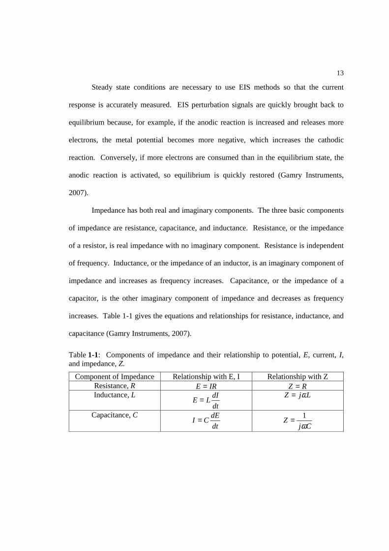
Impedance has both real and imaginary components. The three basic components
of impedance are resistance, capacitance, and inductance. Resistance, or the impedance
of a resistor, is real impedance with no imaginary component. Resistance is independent
of frequency. Inductance, or the impedance of an inductor, is an imaginary component of
impedance and increases as frequency increases. Capacitance, or the impedance of a
capacitor, is the other imaginary component of impedance and decreases as frequency
increases. Table 1-1 gives the equations and relationships for resistance, inductance, and
capacitance (Gamry Instruments, 2007).
Table 1-1: Components of impedance and their relationship to potential, E, current, I, and impedance, Z.
Component of Impedance Relationship with E, I Relationship with Z Resistance, R IRE = RZ = Inductance, L
dt
dILE =
LjZ ω=
Capacitance, C
dt
dECI =
CjZ
ω1=
14
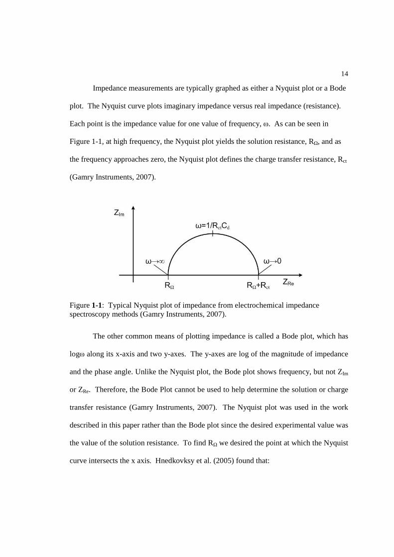
Impedance measurements are typically graphed as either a Nyquist plot or a Bode
plot. The Nyquist curve plots imaginary impedance versus real impedance (resistance).
Each point is the impedance value for one value of frequency, ω. As can be seen in
Figure 1-1, at high frequency, the Nyquist plot yields the solution resistance, RΩ, and as
the frequency approaches zero, the Nyquist plot defines the charge transfer resistance, Rct
(Gamry Instruments, 2007).
The other common means of plotting impedance is called a Bode plot, which has
logω along its x-axis and two y-axes. The y-axes are log of the magnitude of impedance
and the phase angle. Unlike the Nyquist plot, the Bode plot shows frequency, but not ZIm
or ZRe. Therefore, the Bode Plot cannot be used to help determine the solution or charge
transfer resistance (Gamry Instruments, 2007). The Nyquist plot was used in the work
described in this paper rather than the Bode plot since the desired experimental value was
the value of the solution resistance. To find RΩ we desired the point at which the Nyquist
curve intersects the x axis. Hnedkovksy et al. (2005) found that:
Figure 1-1: Typical Nyquist plot of impedance from electrochemical impedance spectroscopy methods (Gamry Instruments, 2007).
15
from the calibration data on KCl and H2SO4, it is evident that the charge transfer resistance is approximately proportional to the solution resistance, and thus, the systematic error caused by the presence of Rct will always be relatively the same so the effect of Rct approximately cancels out (Hnedkovsky et al., 2005).
Therefore, if the ratio of the charge transfer resistance to the solution resistance is
independent of electrolyte concentration, the effect of charge transfer resistance is taken
into account by the cell constant, and, with the relatively small error of 1-2 percent, we
can determine the value of the solution resistance or conductivity independent of the
charge transfer resistance (Hnedkovsky et al., 2005).
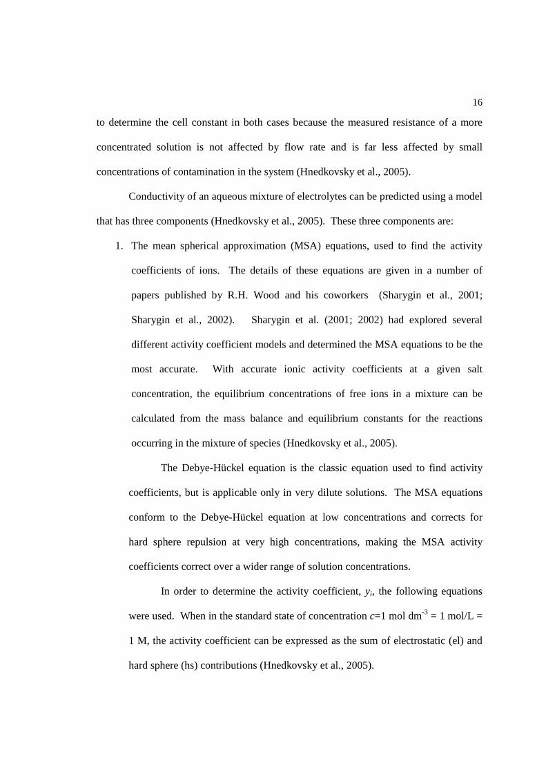
Solution resistance can be found using only a working electrode and a
counter/reference electrode. The conductivity, κ, of the electrolyte is determined using
the equation which was previously noted in the overview of basic concepts of
conductivity (Gamry Instruments, 2007):
where R is the experimentally measured solution resistance measured in Ohms (Ω), A is
the area of the electrodes, l is the distance between the electrodes, and κ is the
conductivity of the solution measured in inverse Ohms per centimeter (Ω-1 cm-1) or
Siemens per centimeter (S cm-1). l/A is known as the cell constant, measured in cm-1, and
can be determined by measuring the resistance of a solution with a well known
conductivity. In this experiment, for the first experimental setup, a solution of 10-2 mol
kg -1 NaCl with known conductivity was used to determine the cell constant. For the
second experimental setup, 3 10-4 mol kg-1 NaCl (aq) solution was used. Solutions with
higher concentrations than the dilute solutions being tested experimentally were chosen
A
l
R
1=κ (1.21)
16
to determine the cell constant in both cases because the measured resistance of a more
concentrated solution is not affected by flow rate and is far less affected by small
concentrations of contamination in the system (Hnedkovsky et al., 2005).
Conductivity of an aqueous mixture of electrolytes can be predicted using a model
that has three components (Hnedkovsky et al., 2005). These three components are:
1. The mean spherical approximation (MSA) equations, used to find the activity
coefficients of ions. The details of these equations are given in a number of
papers published by R.H. Wood and his coworkers (Sharygin et al., 2001;
Sharygin et al., 2002). Sharygin et al. (2001; 2002) had explored several
different activity coefficient models and determined the MSA equations to be the
most accurate. With accurate ionic activity coefficients at a given salt
concentration, the equilibrium concentrations of free ions in a mixture can be
calculated from the mass balance and equilibrium constants for the reactions
occurring in the mixture of species (Hnedkovsky et al., 2005).
The Debye-Hückel equation is the classic equation used to find activity
coefficients, but is applicable only in very dilute solutions. The MSA equations
conform to the Debye-Hückel equation at low concentrations and corrects for
hard sphere repulsion at very high concentrations, making the MSA activity
coefficients correct over a wider range of solution concentrations.
In order to determine the activity coefficient, yi, the following equations
were used. When in the standard state of concentration c=1 mol dm-3 = 1 mol/L =
1 M, the activity coefficient can be expressed as the sum of electrostatic (el) and
hard sphere (hs) contributions (Hnedkovsky et al., 2005).
17
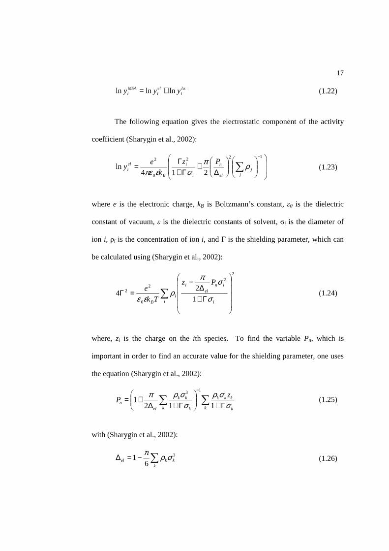
The following equation gives the electrostatic component of the activity
coefficient (Sharygin et al., 2002):
where e is the electronic charge, kB is Boltzmann’s constant, ε0 is the dielectric
constant of vacuum, ε is the dielectric constants of solvent, σi is the diameter of
ion i, ρi is the concentration of ion i, and Γ is the shielding parameter, which can
be calculated using (Sharygin et al., 2002):
where, zi is the charge on the ith species. To find the variable Pn, which is
important in order to find an accurate value for the shielding parameter, one uses
the equation (Sharygin et al., 2002):
with (Sharygin et al., 2002):
hsi
eli
MSAi yyy lnlnln += (1.22)
∆+
Γ+Γ
=−
∑122
0
2
214ln
jj
el
n
i
i
B
eli
Pz
k
ey ρπ
σεπε (1.23)
22
0
22
1
24
Γ+∆
−=Γ ∑
i
inel
i
ii
B
Pz
Tk
e
σ
σπ
ρεε
(1.24)
∑∑ Γ+
Γ+∆+=
−
k k
kkk
k k
kk
eln
zP
σσρ
σσρπ
1121
13
(1.25)
∑−=∆k
kkel3
61 σρπ
(1.26)
18
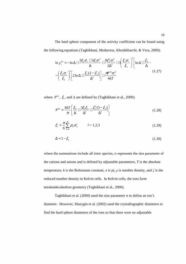
The hard sphere component of the activity coefficient can be found using
the following equations (Taghikhani, Modarress, Khoshkbarchi, & Vera, 2000):
where hsP , lξ , and ∆ are defined by (Taghikhani et al., 2000):
where the summations include all ionic species, σ represents the size parameter of
the cations and anions and is defined by adjustable parameters, T is the absolute
temperature, k is the Boltzmann constant, π is pi, ρ is number density, and ξ is the
reduced number density in Kelvin cells. In Kelvin cells, the ions form
tetrakaidecahedron geometry (Taghikhani et al., 2000).
Taghikhani et al. (2000) used the size parameter σ to define an ion’s
diameter. However, Sharygin et al. (2002) used the crystallographic diameters to
find the hard sphere diameters of the ions so that there were no adjustable
kT
P
y
ihs
i
iiiihsi
6
)2(ln2
ln32
933lnln
3
333
3
3
2
3
2
3
22
222
212
σπξξξσξ
ξξσξσξσξσξ
+
∆−
+∆
−
−
∆+∆
+
∆+
∆+
+∆−=
(1.27)
∆−
+∆
+∆
=3
332
2210 )3(36 ξξξξξ
πkT
P hs (1.28)
∑=
=N
k
lkkl
16σρπξ l = 1,2,3 (1.29)
31 ξ−=∆ (1.30)
19
parameters. The radii of an ion cluster, ric, was found using (Sharygin et al.,
2002):
where rA+ is the crystallographic radii of the cation and rB- is the crystallographic
radii of the anion, and where υi is the number of cations/anions per formula unit
of electrolyte.
Once activity coefficients have been determined, other experimentally
determined thermodynamic data, such as the dissociation constant and the
equilibrium constant can be used in conjunction with the activity of a species to
determine the concentration of each species present at a given temperature and
pressure. Knowing the concentration of each species is necessary in determining
the next component of the conductivity model, the conductivity of a single
electrolyte.
2. The Turq – Bernard – Blum – Kunz (TBBK) equation, used to find the equivalent
conductivity of a single strong electrolyte as a function of concentration
(Hnedkovsky et al., 2005). Sharygin et al. (2001) had explored several models
for the conductivity of a single strong electrolyte and found the TBBK model was
applicable with reasonable accuracy across a temperature range from 25 to
300°C. Wood and coworkers confirmed the TBBK equation in its application to
NaCl (aq) solutions up to 1 mol kg-1 at 400°C (28 MPa), and for KCl (aq)
solutions up to 4.5 mol kg-1 at 300-600°C (100-300 MPa) (Sharygin et al., 2002).
3 32
31 −+ += BAic rvrvr (1.31)
20
The Debye-Hückel-Onsager equation to determine the conductivity of
dilute electrolyte solutions is a classical equation to determine electrolyte
conductivity at a given concentration by adjusting the limiting molar ionic
conductivity to account for the relaxation effect and the electrophoretic effect
(Hamann et al., 1998). The TBBK method uses a similar approach but extends
the concentration range of the Debye-Hückel-Onsager equation. For the TBBK
model, the molar conductivity of a single electrolyte solution, ΛF, with two types
of free ions is given by (Sharygin et al., 2002):
where the molar conductivity of ion i, λiF, is given by (Sharygin et al., 2002):
for which, 0iλ is the limiting equivalent molar conductivity at infinite dilution,
0/ ieli vvδ is the free ion electrophoretic velocity effect, δX/X is the free ion
relaxation force correction, and viO is the ion velocity at infinite dilution in
electric field E, which is defined by the equation (Sharygin et al., 2002):
FFF 21 λλ +=Λ (1.32)
+
+=
X
X
v
v
i
eli
iFi
δδλλ 110
0 (1.33)
Tk
Dev
B
iii
00 E= (1.34)
21
where ei = zie is the electric charge of the ith ion, E is the electric field, and Di0 is
the diffusion coefficient of the ith ion at infinite dilution, which is given by
(Sharygin et al., 2002):
where F is Faraday’s constant.
Within the TBBK model, qκ defines the influence of absolute ion
mobility on molar conductivity. For a 1-1 electrolyte like NaCl, qκ -1 is equal to
the Debye screening length, which was previously defined. In this case, the qκ
does not depend on individual ion mobility, and the molar conductivity depends
on sum of equivalent ion conductivities at infinite dilution but not on their
difference. qκ is defined by (Sharygin et al., 2002):
3. A mixing rule, used to predict the molar conductivity of mixtures of strong
electrolytes based upon the molar conductivity of single component electrolytes
(Hnedkovsky et al., 2005). It was demonstrated by Sharygin et al. (2001) that
there is a general mixing rule that was given in several papers by different
authors, and this rule contained the same essential components. The chosen
mixing rule, given by Reilly and Wood (1969), is similar to the mixing rule of
Anderko and Lencka (1997) and is a similar, but more generalized version of the
2
00
Fz
RTD
i
ii
λ= (1.35)
00
0202
0
22
ji
jjjiii
Bq
DD
DzDz
Tk
e
++
=
ρρεε
κ (1.36)
22
mixing rule tested by Miller and Young and coworkers (Wu, Smith, & Young,
1965; Young & Smith, 1954).
The equation for determining the conductivity, κ, of a solution with molar
ionic strength, Ic, is (Sharygin et al., 2002):
where Nc and Na are, respectively, the numbers of cations and anions in the
mixture, x is the equivalent fractions of species in solution define by xM= cMzM/N
and xX=cX|zX|/N, c is the concentration in mol dm-3 = mol L-1, zi is the charge on
the ith species, and N is the equivalent concentration defined by (Sharygin et al.,
2002):
with summations over all cations M and all anions X. ΛMX is an electrolyte’s
molar conductivity calculated at molar ionic strength, Ic, where (Sharygin et al.,
2002):
][][1 1
c
N
M
N
XMXXMc IxxNI
c a
∑∑= =
Λ=κ (1.37)
∑∑ == XXMM zczcN (1.38)
2
22 ∑∑ += XXMM
c
zczcI (1.39)
23
1.3 Literature Review
1.3.1 Previous high temperature conductivity measurements of NaCl (aq)
Although electrical conductivity measurements at ambient temperature and
pressure predominate in the industries that use electrochemical conductivity sensors, such
as power plants, high temperature and pressure conductivity measurements were
pioneered by Noyes et al. in the early 1900s. Noyes’ work included the study of high
temperature NaCl (aq) solutions (Noyes, 1907). Later, Marshall and Franck and
coworkers obtained important data on the electrical conductivity of NaCl (aq) solutions at
Oak Ridge National Laboratory (ORNL). Marshall and Quist studied the conductivity of
solutions from the ambient to supercritical range (A. S. Quist, 1970; A. S. Quist & W. L.
Marshall, 1968). In the early 1960’s, Franck, Marshall, and others built an apparatus at
ORNL to measure conductivity at high temperatures and pressures (Franck, Savolainen,
& Marshall, 1962; A. S. Quist, Jolley, Marshall, & Franck, 1963). This instrument
allowed measurements to be taken in conditions up to 800°C and 400 MPa (Mesmer et
al., 1997).
1.3.2 Modern conductivity measurements of NaCl (aq)
The instrument built and designed by Franck, Marshall, and others (Franck et al.,
1962; A. S. Quist et al., 1963) was later modified by Ho and Palmer (Ho & Palmer, 1995;
Ho, Palmer, & Mesmer, 1994) to improve the apparatus’s temperature control and
24
measurement capabilities. The apparatus was then limited to temperatures up to 650°C
and pressures up to 300 MPa (Mesmer et al., 1997).
At ORNL, Ho and Palmer (1995; 1994) obtained NaCl (aq) data, modeling its
conductance at and near the supercritical region. Ho and Palmer (1995; 1994) used the
Shedlovsky or Fuoss and Hsia conductance equations to fit data and obtain the
association constant of NaCl (aq).
In 1995 Zimmerman, Guszkiewics and Wood (1995) had built the first flow-
through conductance cell that was capable of functioning at the critical temperature of
pure water (Ho, Bianchi, Palmer, & Wood, 2000). Zimmerman et al. (1995) measured
the conductivity of dilute NaCl (aq) solutions at high temperatures and pressures, and the
results of that data proved consistent with previous research by Noyes (1907) and
Pearson et al. (1963). The methodology used by Zimmerman et al. (1995) was used by
Gruszkiewicz and Wood (1997) to obtain conductivity data on dilute NaCl solutions at
supercritical conditions, and the results compared favorably to the data of Fogo et al.
(1954) and Pearson et al. (1963). The overall consistency of this experimental data on
the conductivity of NaCl (aq) is important because this data was later used by R. H.
Wood and coworkers as validation for a three component model for predicting the
conductivity of electrolyte mixtures (Hnedkovsky et al., 2005; Sharygin et al., 2001;
Sharygin et al., 2002).
The instrument used at ORNL employed a static high-pressure cell, and in order
to obtain accurate measurements for the dilute solutions, a flow-through cell was
necessary (Ho et al., 2000). Ho and Palmer teamed up with R. H. Wood and co-workers
at the University of Delaware to create a flow-through electrical conductance cell at
25
ORNL (Ho et al., 2000). Ho et al. (2000) tested the conductivity of several dilute
electrolytes, including NaCl (aq). It was found that the conductivity data for NaCl (aq)
measured by Ho et al. (2000) agreed with the earlier experimental data of Ho and Palmer
(1995; 1994) and the experimental data of Zimmerman et al. (1995).
1.3.3 Theoretical analysis of conductivity data
In 1995, after using the new high temperature and pressure flow-through
conductance cell to obtain experimental NaCl (aq) conductivity data at and near the
critical point of water, Zimmerman et al. (1995) used their data on NaCl (aq) conductivity
to test the Fuoss-Hsia-Fernández-Prini (FHFP) model for describing the dependence of
the dilute 1:1 electrolyte’s equivalent molar conductivity on concentration and found the
model to be accurate for NaCl (aq) data. The Fuoss-Hsia-Fernández-Prini (FHFP) model
is based upon the theoretical treatment of Fuoss and Hsia (1967) and equations given by
Fernandez-Prini (1969). Viscosity was determined using a compilation of data from
Johnson and Norton (1991).
Sharygin et al. (2001) later tested equations to calculate the conductivity of
mixtures of ions in aqueous solutions at high temperatures. The conductivities resulting
from these equations were tested against the experimental NaCl (aq) data measured by
Gruszkiewicz and Wood (1997) and against the theoretical equation by Durand-Vidal et
al. (1996) for three ion mixtures. Sharygin et al. (2001) also tested the equations against
their own experimental data on Na2SO4 (aq). The experimental results and calculated
conductivities were found to be in agreement. Sharygin et al. (2001) showed that
26
conductivity measurements can yield accurate equilibrium constants in complex mixtures
of ions. Sharygin et al. (2001; 2002) had explored several different activity coefficient
models, models for the conductivity of a single strong electrolyte, and an equation
determined by Reilly and Wood (1969) for obtaining the conductivity of ionic mixtures.
To find the conductivity of a strong electrolyte as a function of concentration, Sharygin et
al. (2001) tested the FHFP model and the Turq, Blum, Bernard, and Kunz (TBBK)
model, which expanded upon the same basic theories used in the FHFP model and was
developed by Turq et al. (1995). The TBBK model was found to be reasonably accurate
for ionic mixtures. The TBBK model, the mixing rule, and the mean spherical
approximation of activity coefficients developed by Blum and Høye (1977) were again
proved to be accurate when compared to experimental data by Sharygin et al. (2002) and
Hnedkovsky et al. (2005). Hnedkovsky et al. (2005) successfully applied the model
developed by Sharygin et al. (2001) for determining the conductivity of electrolyte
mixtures and showed that for dilute solutions (with molality below 0.016) the equations
gave satisfactory fits to the experimental conductivity data, so this model has been shown
to be applicable for the dilute solutions being tested in this thesis.
1.3.4 Instruments for in situ conductivity measurements of high temperature/high pressure aqueous solutions
Asakura et al. (1989) had designed an in-line conductivity monitor to aid in the
determination of impurities in boiler water. However, their design employed poly-
tetrafluorethylene (PTFE) directly in the electrode assembly, and PTFE, a type of
Teflon®, is known to be unstable above approximately 250°C (Balashov et al., 2007).
27
Asakura et al. (1989) also did not have had access to the breakthroughs made by R.H.
Wood and co-workers in determining the conductivity of electrolyte mixtures
(Hnedkovsky et al., 2005; Sharygin et al., 2006; Sharygin et al., 2001; Sharygin et al.,
2002). In the report of Asakura et al. (1989), deviations of the experimental conductivity
from the predicted conductivity were particularly notable above 200°C.
According to Larson, Olson, & Lilley (2007), in a paper that was submitted in
February of 2006, at that time there was no sensor capable of measuring chloride
concentration under in situ conditions on a long-term basis other than their own. Larson
et al. (2007) had developed an oceanographic application for their high temperature and
pressure sensor, which was capable of withstanding temperatures up to 380°C and
pressures up to 30 MPa; their probe was developed for deployment into deep-sea
hydrothermal vents. Larson et al. (2007) used measurements of solution resistance to
determine the concentration of NaCl (aq), or chloride. The probe employed four gold
ball electrodes, which functioned in pairs and were pressed into a magnesium stabilized
ZrO2 ceramic rod creating a gold/ceramic seal (Larson et al., 2007). The wire leads were
ceramic-insulated and housed in a pressure compensated titanium wand. Beyond the
wand, the wires were enclosed in a Tygon-tube containing non-conductive oil and then
attached to a deep-sea cable. Temperature measurements were taken using a
thermocouple which was attached to the outside of the wand (Larson et al., 2007). This
device shows some distinct similarities to the device described in this thesis. Both
apparatuses were devised for use in high temperature and pressure in-situ conditions and
both determine concentration of NaCl using conductivity measurements. However, due
to the emphasis of oceanography specifically on oceanic chloride concentrations, Larson
28
et al. (2007) have specialized in the change of conductivity with temperature of a specific
solution of NaCl mixed with a given concentration of K+ and Ca+2 ions that is typical in
the Main Endeavour Field hydrothermal vents. Their approach to determining the
dissolved chloride concentration from conductivity data is based on the empirical
treatment of experimental conductivities of high temperature aqueous mixtures of NaCl
and other alkali metal halides performed by Quist and Marshall (A.S. Quist & W.L.
Marshall, 1968; A.S. Quist & Marshall, 1969). The work done in this thesis was not
based upon purely empirical formulas; instead, the concentration of chloride was
determined by taking experimental conductivity measurements and comparing these
conductivities to the theoretically calculated conductivity of aqueous electrolyte mixtures
from the progressive models developed by R. H. Wood and co-workers (Hnedkovsky et
al., 2005; Sharygin et al., 2006; Sharygin et al., 2001; Sharygin et al., 2002). Due to the
flexibility of this model, our data treatment is more versatile than the treatment performed
by Larson et al. (2007). Larson et al. (2007) also considered more concentrated NaCl
(aq) solutions, from 0.054 to 3 mol kg-1, whereas our device was used to determine the
concentration of much more dilute NaCl (aq) solutions, which have historically presented
difficulties in electrical conductivity measurements.
Chapter 2
Experimental Techniques
A series of probe designs and experimental measurements resulted in testing two
probes in two different systems. In the first experimental setup, a flow-through probe
with two platinum black electrodes was tested in the “T” cell system, in a high
temperature flow-through electrochemical cell designed and available in our Laboratory
(Lvov, 2007; Lvov & Zhou, 1998; Lvov, Zhou, & Macdonald, 1999; Lvov et al., 2003).
In the second experimental setup, a flow-through probe originally designed for corrosion
studies with a steel working electrode and gold reference electrode was tested in a new
flow-through tubular reactor system available in our Laboratory. The changes were made
from the first to the second system due to experimental problems with the first system,
namely contamination in the conductivity measurements, difficulty regulating
temperature, and the large volume of the “T” cell system. The change in probes was
made due to contamination problems. Possible reasons for these contaminations
problems include the alumina in the platinum probe, the necessity of testing the
conductivity applications of a corrosion probe that was also designed for EPRI, and
because one of the Pt leads in the first probe was irreparably damaged. The two probes
were similar; both conductivity probes were designed on the basis of the working/counter
(w/c) electrode assembly developed in our Laboratory for the EPRI Corrosion Project
(Lvov, Fedkin, & Balashov, 2005). Both were flow-through probes with a Conax gland
30
connector and annular duct geometry for the electrodes, and both could be used
interchangeably in either experimental system.
2.1 Preparation of Solutions
Solutions were made using purified, de-ionized water, with a resistivity of 18.2
MΩ·cm, from a Milli-Q® ultrapure water purification system. NaCl solutions were made
from crystal sodium chloride of 99.9% purity from J. T. Baker, and the AVT solutions
were made from 0.1 mol L-1 ammonium hydroxide standard solution from Alfa Aesar.
The deoxygenated AVT regime for power plant boilers has minimal oxygen
content in order to prevent the formation of iron oxides causing the corrosion of steel
pipes and boilers. The composition of the solutions that were studied was based on the
targeted AVT specifications, so dilute deoxygenated NH4OH - H2O and NaCl - NH4OH -
H2O aqueous solutions with a pH of 9 were the test solutions and were prepared as
follows. The 20 liter Nalgene solution tank, calibrated to ± 0.1 liter, was purged with
argon for at least one hour and then filled with ultra-pure de-ionized Milli-Q water with a
resistivity of 18.2 MΩ.cm under an argon atmosphere. The argon kept the solution
deoxygenated by preventing its contact with air. The prepared solution was kept under
an argon atmosphere throughout the experiment by continuously bubbling argon through
the test solution. By using this procedure, the oxygen concentration was kept in the range
of 5-10 ppb. The oxygen content in the working solution was measured by colorimetric
analysis (CHEMets K-7501and K-7540).
31
To prepare the AVT solution, 4.0 ml of 0.1 mol L-1 NH4OH (Alfa Aesar
standardized solution) was injected to the 20 liter tank of Milli-Q water using a syringe.
The pH of the solution was monitored by removing a solution sample through a side
outlet in the tank and immediately placing the solution in a Cole Palmer high precision
glass pH electrode at room temperature. The electrode was left in the solution for several
minutes because the pH reading continued to increase and did not reach equilibrium for
several minutes. For solutions containing chloride, the necessary concentrations of 10-2
mol kg-1 NaCl stock solution were injected with a syringe. The conductivity of the
working solution was monitored at room temperature and pressure with an auxiliary high
precision standard Milli-Q resistivity flow cell obtained from the Millipore Corporation.
This measurement was taken to ensure that the conductivity of the solution under
atmospheric conditions matched the calculated conductivity of our test solution before
the solution entered the experimental system.
2.2 Conductivity Measurements
All conductivity measurements were made using a Gamry Instruments system,
which included a Gamry PC4-750TM Potentiostat and Gamry Instruments Framework
Version 4.35 software.
One of the main obstacles to accurately carrying out high temperature
conductivity measurements of very dilute solutions is the ionic contamination from the
instrument being used to take conductivity measurements. The contamination from the
instrument should be determined from the conductivity measurements of pure, de-ionized
32
water and then be subtracted from the experimental conductivities to determine the actual
conductivities of the solutions in the following manner (Hnedkovsky et al., 2005;
Sharygin et al., 2001):
where measuredκ is the measured specific conductivity of the solution, corrκ is the corrected
value of conductivity of the solution, and ..iiκ is the conductivity of instrumental ionic
impurity. The instrumental ionic contamination ..iiκ is defined by:
where obswκ is the experimental conductivity of pure de-ionized water, and wκ is the
calculated, theoretical conductivity of pure de-ionized water.
If experimental data has been adjusted to account for the total ionic
contamination, the fact will be noted.
All theoretical, calculated conductivities in this thesis have been calculated using
the conductivity model with three components as it was developed and described by R.H.
Wood and co-workers: Hnedkovsky et al. (2005) and Sharygin et al. (2006; 2001; 2002).
For the experiments presented in this thesis, the experimental solutions were pure water,
the AVT solution, and dilute NaCl solutions in NH4OH (aq) corresponding to the AVT
solution.
For the solutions of dilute NaCl in the AVT solution, the additives to pure water
were NaCl and NH4OH, causing 6 reactions and 11 species, which were used in the
calculations. The reactions used were:
..iimeasuredcorr κκκ −= (2.1)
wobswii κκκ −=.. (2.2)
33
The dissociation constant of NaCl was obtained from the empirical polynomial
function of water density and temperature given by Balashov (Balashov, 1995). The
dissociation constant of water was calculated using the equation developed by Bandura
and Lvov (Bandura & Lvov, 2006). Data for the AVT solution, or NH4OH – H2O
system, was obtained from Quist and Marhsall (1968), Robinson and Stokes (1959), and
Marshall (1987).
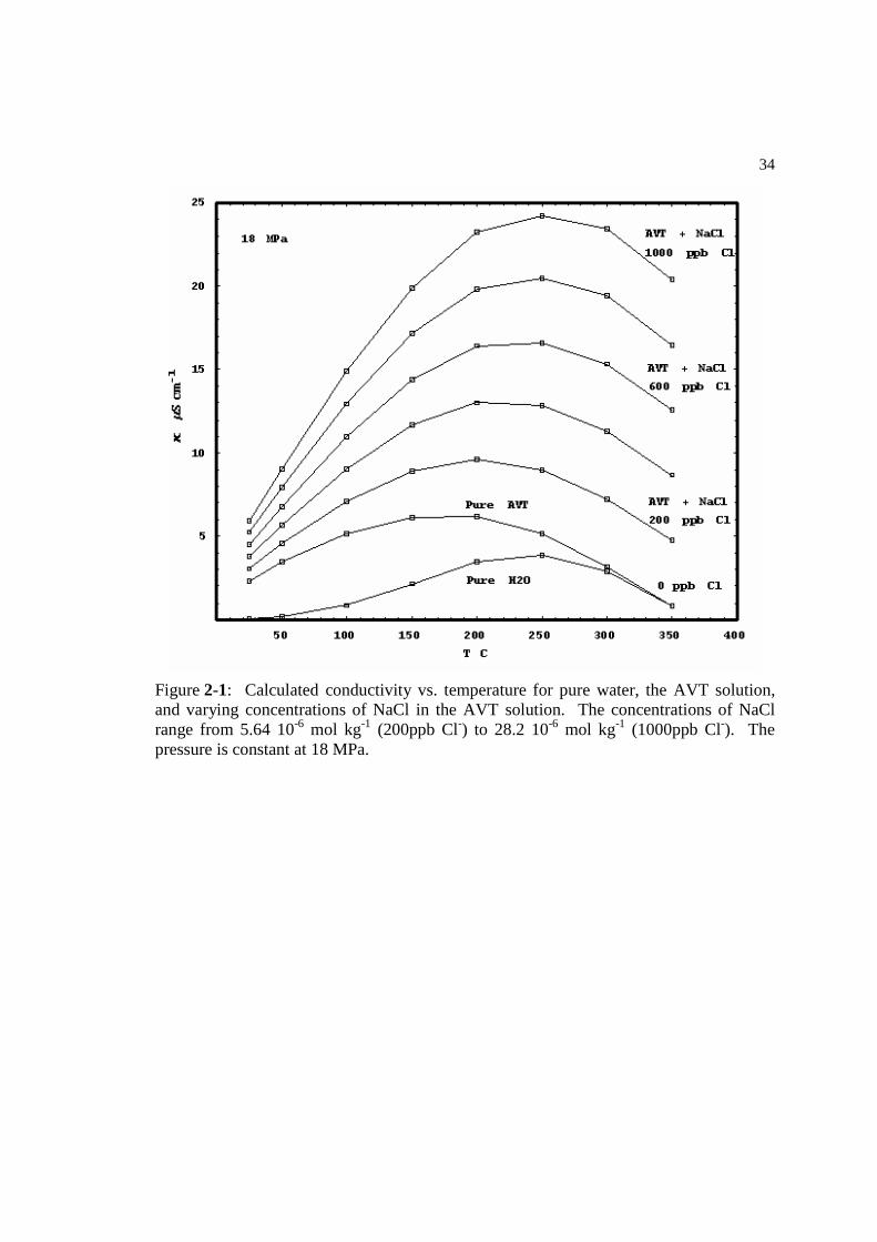
The theoretical conductivities of pure water, the AVT solution, and a range of
dilute NaCl solutions in the AVT regime were calculated (see Figure 3-1).
OH- + H+ = H2O (2.3)
HCl = H+ + Cl- (2.4)
NaCl = Na+ + Cl- (2.5)
NaOH = Na+ + OH- (2.6)
NH4Cl = NH4+ + Cl- (2.7)
NH4OH = NH4+ + OH- (2.8)
34
Figure 2-1: Calculated conductivity vs. temperature for pure water, the AVT solution, and varying concentrations of NaCl in the AVT solution. The concentrations of NaCl range from 5.64 10-6 mol kg-1 (200ppb Cl-) to 28.2 10-6 mol kg-1 (1000ppb Cl-). The pressure is constant at 18 MPa.
Chapter 3
First Experimental System
3.1 Probe Design and Experimental Setup for First Experimental System
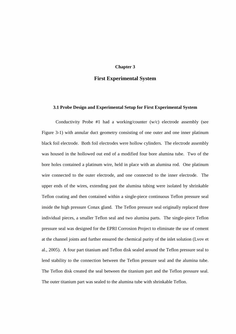
Conductivity Probe #1 had a working/counter (w/c) electrode assembly (see
Figure 3-1) with annular duct geometry consisting of one outer and one inner platinum
black foil electrode. Both foil electrodes were hollow cylinders. The electrode assembly
was housed in the hollowed out end of a modified four bore alumina tube. Two of the
bore holes contained a platinum wire, held in place with an alumina rod. One platinum
wire connected to the outer electrode, and one connected to the inner electrode. The
upper ends of the wires, extending past the alumina tubing were isolated by shrinkable
Teflon coating and then contained within a single-piece continuous Teflon pressure seal
inside the high pressure Conax gland. The Teflon pressure seal originally replaced three
individual pieces, a smaller Teflon seal and two alumina parts. The single-piece Teflon
pressure seal was designed for the EPRI Corrosion Project to eliminate the use of cement
at the channel joints and further ensured the chemical purity of the inlet solution (Lvov et
al., 2005). A four part titanium and Teflon disk sealed around the Teflon pressure seal to
lend stability to the connection between the Teflon pressure seal and the alumina tube.
The Teflon disk created the seal between the titanium part and the Teflon pressure seal.
The outer titanium part was sealed to the alumina tube with shrinkable Teflon.
36
Due to the Teflon coating on the wires and the alumina rods, the electrodes were
exposed to the experimental solution only in the target-temperature zone at the electrode
assembly. The solution flowed through the two remaining bore holes until it reached the
electrode assembly and flowed between the two cylindrical electrodes. The Teflon
pressure seal had the electrode terminals and the solution inlet capillary running through
it. The electrode terminals were connected to the Gamry system, and the capillary was
connected to a high pressure chromatography pump (Acuflow Series II Pump), which
does not contain any metallic parts. Thus, until reaching the electrode assembly, the
prepared solution was only in contact with Teflon and PEEK (polyether ether ketone)
tubes at ambient temperature and with alumina ceramics at elevated temperatures (Lvov
& Fedkin, 2004).
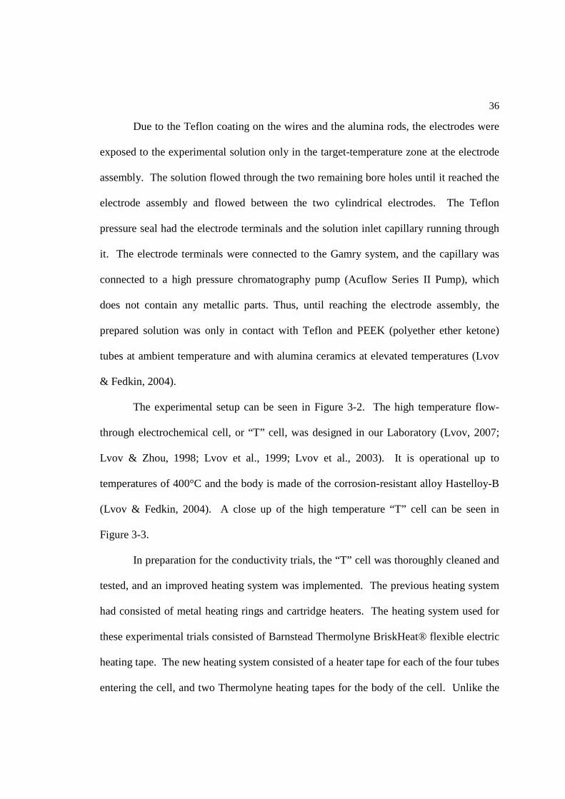
The experimental setup can be seen in Figure 3-2. The high temperature flow-
through electrochemical cell, or “T” cell, was designed in our Laboratory (Lvov, 2007;
Lvov & Zhou, 1998; Lvov et al., 1999; Lvov et al., 2003). It is operational up to
temperatures of 400°C and the body is made of the corrosion-resistant alloy Hastelloy-B
(Lvov & Fedkin, 2004). A close up of the high temperature “T” cell can be seen in
Figure 3-3.
In preparation for the conductivity trials, the “T” cell was thoroughly cleaned and
tested, and an improved heating system was implemented. The previous heating system
had consisted of metal heating rings and cartridge heaters. The heating system used for
these experimental trials consisted of Barnstead Thermolyne BriskHeat® flexible electric
heating tape. The new heating system consisted of a heater tape for each of the four tubes
entering the cell, and two Thermolyne heating tapes for the body of the cell. Unlike the
37
previous heating system, the new system did not contain any metallic parts and more
fully covered the exterior of the “T” cell. After the new heating system was
implemented, the cell was well insulated to maximize heating efficiency.
Figure 3-1: Conductivity Probe #1, with platinum black electrodes. Figure is not to scale.
38
Figure 3-2: First experimental system setup, “T” cell system. Figure is not to scale.
39
3.2 Observed Data for First Experimental System
Before measuring the conductivity of dilute NH4OH/NaCl aqueous solutions, the
cell constant of Probe #1 was found. The theoretical conductivity of 10-2 mol kg -1 NaCl
was calculated using the algorithms developed by Sharygin et al. (2001) and Hnedkovsky
et al. (2005). The theoretical conductivity of 10-2 mol kg -1 NaCl at 10MPa and 25.0°C
was determined to be 1206.91 µS cm-1. The resistance of the 10-2 mol kg -1 NaCl solution
was experimentally determined at atmospheric temperature, at a pressure of 10 MPa, and
Figure 3-3: High temperature and high pressure electrochemical “T” cell. Figure is not to scale.
40
at a flow rate of 5 cm3/min (see Table 3-1). The cell constant of Probe #1 was
determined to be 0.0607 cm-1.
The conductivity of three solutions was measured at 25°C, 100°C, 200°C, 300°C,
and 350°C. All measurements were taken at a pressure of approximately 18 MPa and at a
flow rate of 6 cm3 min-1. After a temperature change, the system was allowed to reach
equilibrium for 2-3 hours. Measurements were taken as the temperature of the system
was increasing to 350°C and then conductivity measurements were repeated as the
temperature was decreasing back to 25°C. Measurements were determined to be
consistent at a given temperature independent of whether the temperature setting for the
system was being increased or decreased. The solutions tested were (1) pure de-ionized
water, (2) the AVT solution that consisted of 1 10-5 mol kg-1 NH4OH, and (3) 6.02 10-6
mol kg-1 NaCl (214 ppb of Cl-) in the AVT solution. Table 3-2 gives the experimental
data, and Figure 3-4 gives a graphical representation of the experimental data given in
Table 3-2 as compared to the theoretical values calculated using the conductivity model
with three components (Hnedkovsky et al., 2005; Sharygin et al., 2001; Sharygin et al.,
2002).
Table 3-1: Experimental resistances of 10-2 mol kg -1 NaCl used to determine the cell constant of the platinum conductivity probe (Probe #1) in the “T” cell system. Flow rate was constant at 6 cm3 min-1.
T (°C) P (MPa) flow rate (cm3/min) R (Ohm) 25.0 10 5 50.09 25.1 11 5 50.27 25.0 10 5 50.31
41
Table 3-2: Experimental resistances and conductivities of Milli- Q water, the AVT solution, and 6.02 10-6 mol kg-1 NaCl in the AVT solution. Measurements were taken using the platinum conductivity probe (Probe #1) in the “T” cell system. Flow rate was constant at 6 cm3 min-1.
T(°C) P
(MPa) Solution R (kΩ) Conductivity
(µS/cm) 25 18.4 Milli-Q water 270.9 0.22 25 18.1 Milli-Q water 273.9 0.22 100 18.3 Milli-Q water 19.69 3.08 99.5 18.3 Milli-Q water 18.23 3.33 200 17.9 Milli-Q water 10.19 5.96 300 17.9 Milli-Q water 4.839 12.54 350 17.9 Milli-Q water 3.936 15.42
300.8 18.1 Milli-Q water 4.892 12.41 99 18.3 Milli-Q water 17.81 3.41 25 18.1 AVT 26.91 2.26 100 17.8 AVT 11.18 5.43
199.9 18.1 AVT 7.092 8.56 300 18.1 AVT 5.758 10.54
349.8 18.3 AVT 4.719 12.86
25 18 6.02 10-6 mol kg-1 NaCl in AVT
20.38 2.98
100 18 6.02 10-6 mol kg-1 NaCl in AVT
8.35 7.27
200.3 18 6.02 10-6 mol kg-1 NaCl in AVT
5.421 11.2
300 18 6.02 10-6 mol kg-1 NaCl in AVT
4.413 13.76
349.8 18 6.02 10-6 mol kg-1 NaCl in AVT
3.827 15.86
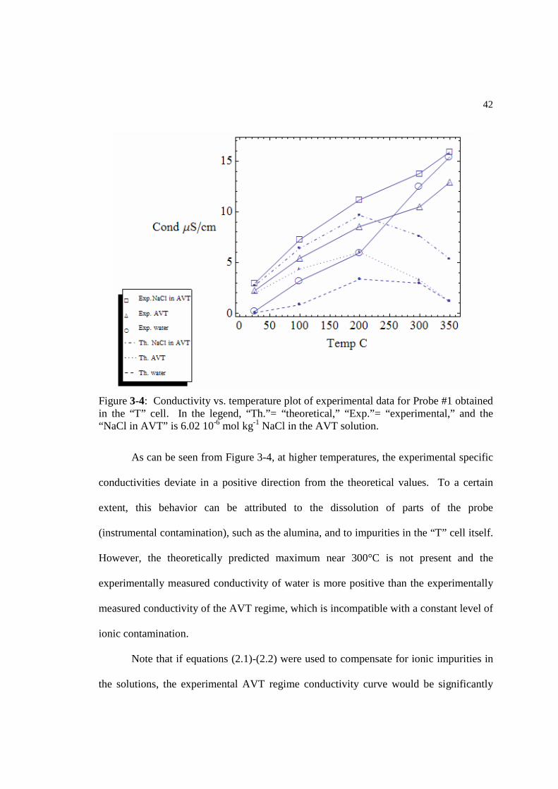
42
As can be seen from Figure 3-4, at higher temperatures, the experimental specific
conductivities deviate in a positive direction from the theoretical values. To a certain
extent, this behavior can be attributed to the dissolution of parts of the probe
(instrumental contamination), such as the alumina, and to impurities in the “T” cell itself.
However, the theoretically predicted maximum near 300°C is not present and the
experimentally measured conductivity of water is more positive than the experimentally
measured conductivity of the AVT regime, which is incompatible with a constant level of
ionic contamination.
Note that if equations (2.1)-(2.2) were used to compensate for ionic impurities in
the solutions, the experimental AVT regime conductivity curve would be significantly
Figure 3-4: Conductivity vs. temperature plot of experimental data for Probe #1 obtained in the “T” cell. In the legend, “Th.”= “theoretical,” “Exp.”= “experimental,” and the “NaCl in AVT” is 6.02 10-6 mol kg-1 NaCl in the AVT solution.
43
more negative than the theoretical, calculated curve corresponding to the chemistry of the
AVT solution. One possible reason that the level of ionic contamination did not remain
constant was that impurities remained in the “T” cell after it was cleaned. The “T” cell
had been in use for many years, so there was the possibility of a continual build up of
impurities from the previous experiments (Lvov & Zhou, 1998; Lvov et al., 1999; Lvov
et al., 2003). The level of impurities would have decreased due to the constant flow of
water during the first trial. Heating the “T” cell for the high temperature measurements
of pure water may have helped further release contaminants in the system, which would
both increase the experimental conductivity measurements of pure water since it was the
first trial and decrease the experimental conductivity measurements of the AVT regime
since it was the second trial and therefore in a cleaner system.
The problem of possible remaining contamination within the cell and problems
with the design of the “T” cell itself, such as difficulty maintaining a constant
temperature in the “T” cell due to the large volume of the cell and due to the high
incoming flow rate of unheated solution, led to the decision to move conductivity
measurements to a second system. The “T” cell’s large volume also meant that it was
difficult to fully eliminate a solution from the body of the cell, so impurities left in the
system from previous test solutions could cause deviations from the expected
conductivity.
The second system had better thermal regulation and a smaller volume than the
“T” cell system, making measurements more accurate and better regulated. Fully
cleaning the “T” cell system was difficult due to the manner in which it was constructed
with four cylindrical tubes attached to the larger main body of the cell. The main body of
44
the second system was a single high pressure tube, which was easier to clean and less
likely to trap impurities inside the flow area. In addition, the pump in the second system
was upgraded to a Lab Alliance Series 1500 Dual Piston Pump, which has a smoother
flow rate, a greater pressure range, and better accuracy and precision than the “T” cell’s
Acuflow Series II Pump with a single piston.
The change was made from Probe #1 to Probe #2 for several reasons. In Probe
#1, the electrodes were housed at the very end of the alumina tube so that they were in
closer contact with the large volume of solution housed within the “T” cell and
consequently in closer contact with several sources of impurities. In Probe #2, the
electrode assembly was housed further from the tip of the outer alumina tube, so that the
electrode assembly was better isolated from the main body of the system and the solution
in contact with the electrodes was almost solely inlet solution. There was also a possible
problem in Probe #1 with greater dissolution of the alumina tubes than in Probe #2. In
addition, one of the platinum leads in Probe #1 was irreparably damaged as it was
removed from the “T” cell, and Probe #2 allowed the possibility of taking both corrosion
and conductivity measurements with the same probe, which would be beneficial for
usage in a power plant.
Chapter 4
Second Experimental System
4.1 Probe Design and Experimental Setup for Second Experimental System
Conductivity Probe #2 had a w/c electrode assembly (see Figure 4-1) with annular duct
geometry consisting of an outer reference electrode of gold foil, shaped as a hollow
cylinder, and an inner working electrode made of a cylindrical carbon steel SA210A1
rod. This probe was developed for the EPRI Corrosion Project in order to study the
corrosion rate of boilers in power plants, which are made of SA210A1 carbon steel (Lvov
et al., 2005). Gold wire was attached to the gold foil and ran between the inner and outer
alumina tubes, through the body of the probe to a connection with the Gamry Instruments
system. Steel wire connected in a similar fashion to the carbon steel rod electrode,
running through the inner alumina tube for isolation from contact with the gold wire. The
upper ends of the wires, extending past the alumina tubing were isolated by a shrinkable
Teflon coating and then contained within a single-piece continuous Teflon pressure seal
inside the high pressure Conax gland. Shrinkable Teflon was used to connect the Teflon
pressure seal to the alumina tubing and create a seal. The Teflon pressure seal had the
electrode terminals and the solution inlet capillary running through it. The electrode
terminals were connected to the Gamry system, and the capillary was connected to a high
pressure chromatography pump (Lab Alliance Series 1500 Dual Piston Pump), which
does not contain any metallic parts. Thus, until reaching the electrode assembly, the
46
prepared solution was only in contact with Teflon and PEEK ( poly (ether ether ketone) )
tubes at ambient temperature and with alumina ceramics at elevated temperatures (Lvov
& Fedkin, 2004). The experimental setup can be seen in Figure 4-2.
Figure 4-1: Conductivity Probe #2, with carbon steel SA210A1 and gold electrodes. Figure is not to scale and is artificially shortened.
47
Temperature was controlled by two thermocouples attached to MicroOmega®
temperature/process controllers. The first thermocouple was externally attached to a
Thermolyne BriskHeat® heating tape and functioned as a pre-heater for the solution. The
second thermocouple was inside the system, regulating the temperature internally by
adjusting the temperature of a second Thermolyne BriskHeat® heating tape that was
wrapped around the main body of the system.
Figure 4-2: Second experimental system setup.
4.2 Observed Data for Second Experimental System
Two different carbon steel/gold electrode assembly corrosion probes were used to
find the experimental conductivity of several aqueous solutions. The primary probe used
for these experimental trials had a cell constant of 0.074 cm-1. For the purposes of this
paper, since both probes were constructed using the same design (see Figure 4-1), “Probe
#2” will refer generically to the carbon steel/gold corrosion probe used to find the
experimental results given in Table 4-3. Table 4-3 notes if the corrosion probe with a cell
constant of 0.049cm-1 was used for a conductivity measurement.
The cell constant of the corrosion probes was found using a 3 10-4 mol kg-1 NaCl
(aq) solution at atmospheric temperature and at a pressure of 5 MPa. The theoretical
conductivity of 3 10-4 mol kg -1 NaCl was calculated using the algorithms developed by
Sharygin et al. (2001) and Hnedkovsky et al. (2005). The theoretical conductivity of 3
10-4 mol kg -1 NaCl at 5 MPa and 25.0°C was determined to be 37.3928 µS cm-1. Tables
4-1 and 4-2 give the experimental resistance of 3 10-4 mol kg -1 NaCl at atmospheric
temperature, at a pressure of 5 MPa, and at a flow rate of 5 cm3 min-1. The cell constant
of the primary corrosion probe was determined to be 0.074 cm-1. From, Table 4-2, the
cell constant of the secondary corrosion probe was determined to be 0.049cm-1.
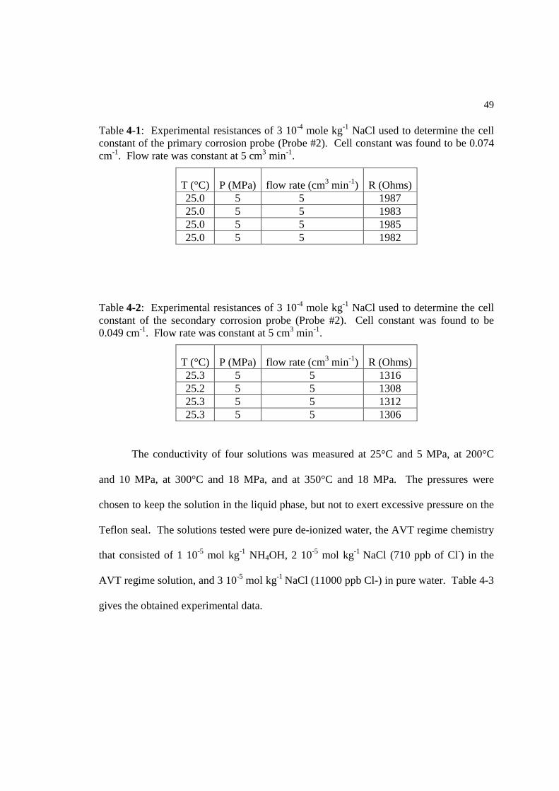
49
The conductivity of four solutions was measured at 25°C and 5 MPa, at 200°C
and 10 MPa, at 300°C and 18 MPa, and at 350°C and 18 MPa. The pressures were
chosen to keep the solution in the liquid phase, but not to exert excessive pressure on the
Teflon seal. The solutions tested were pure de-ionized water, the AVT regime chemistry
that consisted of 1 10-5 mol kg-1 NH4OH, 2 10-5 mol kg-1 NaCl (710 ppb of Cl-) in the
AVT regime solution, and 3 10-5 mol kg-1 NaCl (11000 ppb Cl-) in pure water. Table 4-3
gives the obtained experimental data.
Table 4-1: Experimental resistances of 3 10-4 mole kg-1 NaCl used to determine the cell constant of the primary corrosion probe (Probe #2). Cell constant was found to be 0.074 cm-1. Flow rate was constant at 5 cm3 min-1.
T (°C) P (MPa) flow rate (cm3 min-1) R (Ohms) 25.0 5 5 1987 25.0 5 5 1983 25.0 5 5 1985 25.0 5 5 1982
Table 4-2: Experimental resistances of 3 10-4 mole kg-1 NaCl used to determine the cell constant of the secondary corrosion probe (Probe #2). Cell constant was found to be 0.049 cm-1. Flow rate was constant at 5 cm3 min-1.
T (°C) P (MPa) flow rate (cm3 min-1) R (Ohms) 25.3 5 5 1316 25.2 5 5 1308 25.3 5 5 1312 25.3 5 5 1306
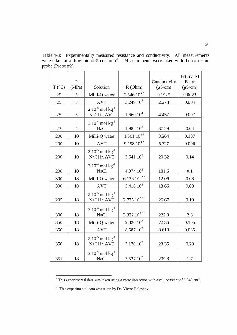
50
* This experimental data was taken using a corrosion probe with a cell constant of 0.049 cm-1.
** This experimental data was taken by Dr. Victor Balashov.
Table 4-3: Experimentally measured resistance and conductivity. All measurements were taken at a flow rate of 5 cm3 min-1. Measurements were taken with the corrosion probe (Probe #2).
T (°C) P
(MPa) Solution R (Ohm) Conductivity
(µS/cm)
Estimated Error
(µS/cm)
25 5 Milli-Q water 2.546 105 * 0.1925 0.0023
25 5 AVT 3.249 104 2.278 0.004
25 5 2 10-5 mol kg-1 NaCl in AVT 1.660 104 4.457 0.007
23 5 3 10-4 mol kg-1
NaCl 1.984 103 37.29 0.04
200 10 Milli-Q water 1.501 104 * 3.264 0.107
200 10 AVT 9.198 103 * 5.327 0.006
200 10 2 10-5 mol kg-1 NaCl in AVT 3.641 103 20.32 0.14
200 10 3 10-4 mol kg-1
NaCl 4.074 102 181.6 0.1
300 18 Milli-Q water 6.136 103 ** 12.06 0.08
300 18 AVT 5.416 103 13.66 0.08
295 18 2 10-5 mol kg-1 NaCl in AVT 2.775 103 ** 26.67 0.19
300 18 3 10-4 mol kg-1
NaCl 3.322 102 ** 222.8 2.6
350 18 Milli-Q water 9.820 103 7.536 0.105
350 18 AVT 8.587 103 8.618 0.035
350 18 2 10-5 mol kg-1 NaCl in AVT 3.170 103 23.35 0.28
351 18 3 10-4 mol kg-1
NaCl 3.527 102 209.8 1.7
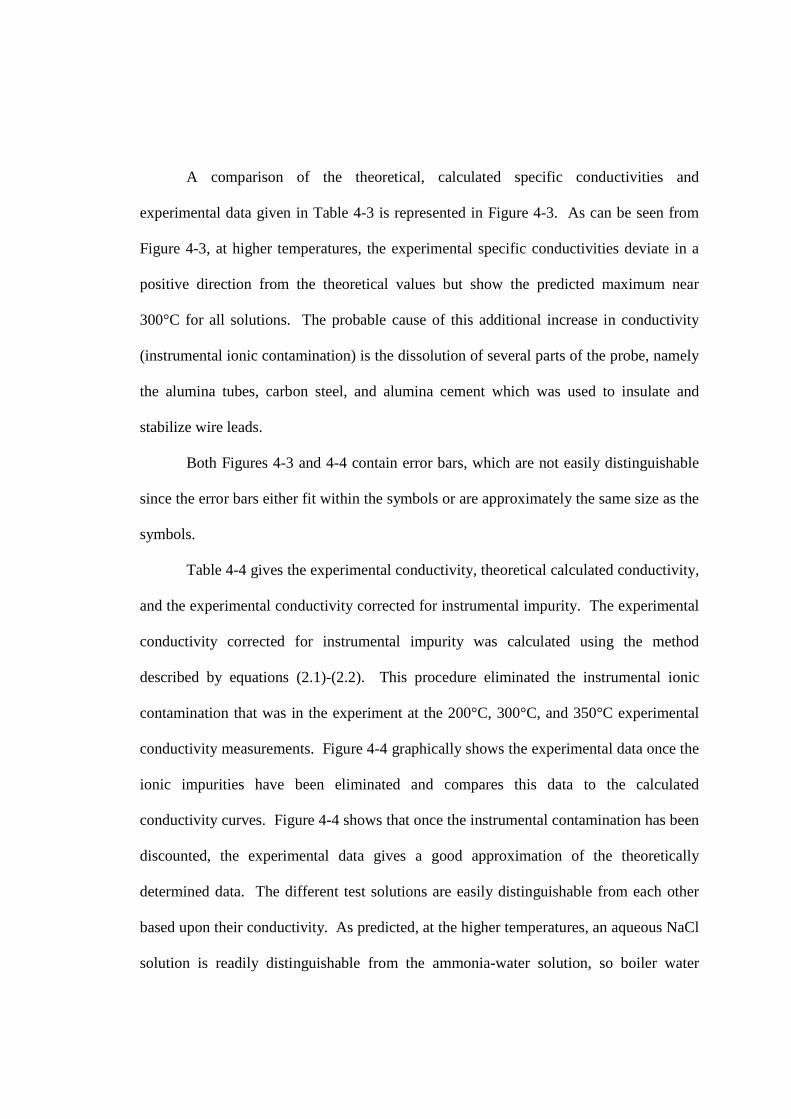
A comparison of the theoretical, calculated specific conductivities and
experimental data given in Table 4-3 is represented in Figure 4-3. As can be seen from
Figure 4-3, at higher temperatures, the experimental specific conductivities deviate in a
positive direction from the theoretical values but show the predicted maximum near
300°C for all solutions. The probable cause of this additional increase in conductivity
(instrumental ionic contamination) is the dissolution of several parts of the probe, namely
the alumina tubes, carbon steel, and alumina cement which was used to insulate and
stabilize wire leads.
Both Figures 4-3 and 4-4 contain error bars, which are not easily distinguishable
since the error bars either fit within the symbols or are approximately the same size as the
symbols.
Table 4-4 gives the experimental conductivity, theoretical calculated conductivity,
and the experimental conductivity corrected for instrumental impurity. The experimental
conductivity corrected for instrumental impurity was calculated using the method
described by equations (2.1)-(2.2). This procedure eliminated the instrumental ionic
contamination that was in the experiment at the 200°C, 300°C, and 350°C experimental
conductivity measurements. Figure 4-4 graphically shows the experimental data once the
ionic impurities have been eliminated and compares this data to the calculated
conductivity curves. Figure 4-4 shows that once the instrumental contamination has been
discounted, the experimental data gives a good approximation of the theoretically
determined data. The different test solutions are easily distinguishable from each other
based upon their conductivity. As predicted, at the higher temperatures, an aqueous NaCl
solution is readily distinguishable from the ammonia-water solution, so boiler water
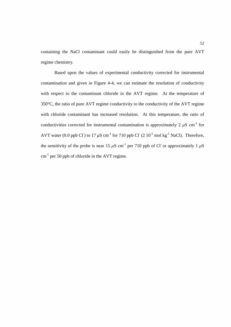
52
containing the NaCl contaminant could easily be distinguished from the pure AVT
regime chemistry.
Based upon the values of experimental conductivity corrected for instrumental
contamination and given in Figure 4-4, we can estimate the resolution of conductivity
with respect to the contaminant chloride in the AVT regime. At the temperature of
350°C, the ratio of pure AVT regime conductivity to the conductivity of the AVT regime
with chloride contaminant has increased resolution. At this temperature, the ratio of
conductivities corrected for instrumental contamination is approximately 2 mS cm-1 for
AVT water (0.0 ppb Cl-) to 17 mS cm-1 for 710 ppb Cl- (2 10-5 mol kg-1 NaCl). Therefore,
the sensitivity of the probe is near 15 mS cm-1 per 710 ppb of Cl- or approximately 1 mS
cm-1 per 50 ppb of chloride in the AVT regime.
53
Figure 4-3: Conductivity vs. temperature plot of experimental data for Probe #2. In the legend, “Th.”= “theoretical,” “Exp.”= “experimental,” and the “NaCl in AVT” is 2 10-5
mol kg-1 NaCl in the AVT solution.
54
Table 4-4: Experimental conductivity, theoretical conductivity, and experimental conductivity corrected for instrumental impurities. Measurements were taken with the corrosion probe (Probe #2).
T (°C)
P (MPa) Solution
Cond. (µS/cm)
Est. Error
(µS/cm)
Theo. Cond.
(µS/cm)
Corr. Cond.
(µS/cm)
Est. Error (µS/cm)
25 5 AVT 2.278 ± 0.004 1.9551 2.142 ± 0.004
25 5
2 10-5 mol kg-1 NaCl in AVT 4.457 ± 0.007 4.4654 4.321 ± 0.007
23 5 3 10-4 mol kg-1 NaCl 37.29 ± 0.04 37.393 37.15 ± 0.04
200 10 Milli-Q water 3.264 ± 0.0023 3.1802 3.180 ± 0.0046
200 10 AVT 5.327 ± 0.006 5.7560 5.243 ± 0.008
200 10
2 10-5 mol kg-1 NaCl in AVT 20.32 ± 0.14 17.881 20.24 ± 0.14
200 10 3 10-4 mol kg-1 NaCl 181.6 ± 0.1 182.80 181.5 ± 0.1
300 18 Milli-Q water 12.06 ± 0.08 2.9719 2.972 ± 0.16
300 18 AVT 13.66 ± 0.08 3.2805 4.572 ± 0.16
295 18
2 10-5 mol kg-1 NaCl in AVT 26.67 ± 0.19 17.670 17.58 ± 0.27
300 18 3 10-4 mol kg-1 NaCl 222.8 ± 2.6 215.13 213.7 ± 2.7
350 18 Milli-Q water 7.536 ± 0.105 1.1513 1.151 ± 0.210
350 18 AVT 8.618 ± 0.035 1.1645 2.233 ± 0.140
350 18
2 10-5 mol kg-1 NaCl in AVT 23.35 ± 0.28 15.076 16.97 ± 0.39
351 18 3 10-4 mol kg-1 NaCl 209.8 ± 1.7 204.45 203.4 ± 1.8
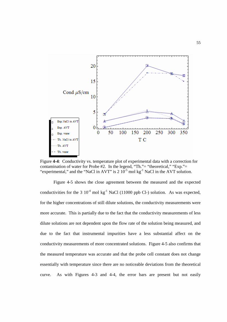
55
Figure 4-5 shows the close agreement between the measured and the expected
conductivities for the 3 10-4 mol kg-1 NaCl (11000 ppb Cl-) solution. As was expected,
for the higher concentrations of still dilute solutions, the conductivity measurements were
more accurate. This is partially due to the fact that the conductivity measurements of less
dilute solutions are not dependent upon the flow rate of the solution being measured, and
due to the fact that instrumental impurities have a less substantial affect on the
conductivity measurements of more concentrated solutions. Figure 4-5 also confirms that
the measured temperature was accurate and that the probe cell constant does not change
essentially with temperature since there are no noticeable deviations from the theoretical
curve. As with Figures 4-3 and 4-4, the error bars are present but not easily
Figure 4-4: Conductivity vs. temperature plot of experimental data with a correction for contamination of water for Probe #2. In the legend, “Th.”= “theoretical,” “Exp.”= “experimental,” and the “NaCl in AVT” is 2 10-5 mol kg-1 NaCl in the AVT solution.
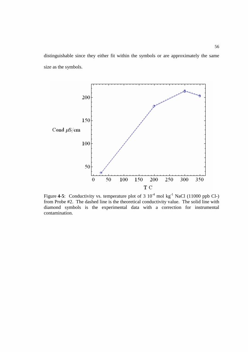
56
distinguishable since they either fit within the symbols or are approximately the same
size as the symbols.
Figure 4-5: Conductivity vs. temperature plot of 3 10-4 mol kg-1 NaCl (11000 ppb Cl-)from Probe #2. The dashed line is the theoretical conductivity value. The solid line with diamond symbols is the experimental data with a correction for instrumental contamination.
Chapter 5
Discussion, Conclusions, and Future Work
5.1 Discussion of Experimental Procedure
The first experimental system did not yield successful results due to problems
with both the “T” cell and the probe, so the system was changed to improve the
performance of the probe. Problems with the “T” cell included its large volume, slow
solution replacement in the cell body, difficulty cleaning the system due to the manner in
which it was constructed, and temperature regulation difficulties particularly at a fast
flow rate. These problems were particularly significant since the experimental solutions
were very dilute. Since dilute solutions are realistic simulations of power plant boiler
water, the second system was implemented and the problems with the “T” cell were
addressed. The second system was easier to cleanse, had a smaller volume and therefore
quicker volume replacement, the temperature was better regulated, and the shape of the
cell was less likely to trap impurities or past solutions in the body of the cell.
Probe #2 with carbon steel and gold electrodes in two single bore alumina tubes
was also an improvement over Probe #1 with platinum black electrodes in a four bore
alumina tube. Due to the difficulty of modifying a four bore alumina tube, the electrode
assembly in Probe #1 was housed closer to the tip of the alumina tube and was therefore
more sensitive to any impurities left in body of the system. In Probe #2, the electrode
assembly was housed further from the tip of the probe, so the alumina tubing provided
58
better insulation from contaminants still in the system. Due to this design, in Probe #2
conductivity measurements were taken when the electrodes were in contact with purer
solution, closer to the inlet. Using Probe #2 for conductivity measurements also showed
that a probe developed for the study of metal corrosion in boilers and boiler pipes could
function to determine conductivity in situ. This is an important conclusion because using
the same probe to study both the corrosion rate of the boiler system and the levels of
impurities in the boiler water would be a useful dual purpose sensor in power plants.
5.2 Conclusions on the Applications of This Experimental Work
From the experimental data produced in the second experimental setup, the
conclusion can be drawn that, using the methods based on the fundamental
thermodynamic and transport data of aqueous species reported by R.H. Wood and his
coworkers, Sharygin et al. (2006; 2001; 2002) and Hnedkovsky et al. (2005), the
measured conductivity of aqueous solutions can be used to predict the electrolyte
composition of boiler water within certain constraints. Those constraints include
knowing the approximate level of NH4OH (aq) present, either through pH measurements
or by recording the amount of NH4OH delivered to the system, and having a
concentration of NaCl (aq) that registers a notable change in conductivity from the
conductivity of pure AVT regime. We have noted that, based on Figure 4-4, at 350°C
Probe #2 has a resolution of approximately 1 mS cm-1 per 50 ppb of chloride in the AVT
regime, and the pure AVT regime has a corrected experimental conductivity of
approximately 2 mS cm-1. Therefore, a change in conductivity due to chloride
59
contamination in the AVT regime should be notable at approximately 50 ppb of chloride
when conductivity is measured at 350°C. Since 50 ppb of chloride is a very dilute
solution, the level of impurities in the boiler water is still very low by the time the
contaminant concentration reaches the point at which it is detectable. Under these
constraints, the experimental work in this thesis has shown that it is possible to predict
the approximate concentration of NaCl present in boiler water by analyzing experimental
conductivity measurements.
After corrections had been made for instrumental impurities, conductivities of
different solutions taken with Probe #2 were readily distinguishable, as shown in Figure
4-4. Probe #2 was therefore successful at determining the concentration of boiler water
contaminant based upon given theoretical conductivities. This was experimentally shown
through conductivity measurements of pure, de-ionized water, the AVT regime, and
2 10-5 mol kg-1 NaCl (710 ppb of Cl-) in the AVT regime solution. These measurements
were taken in a temperature range of 25-350°C and a pressure range of 5-18 MPa. At the
higher temperatures, the AVT regime was more readily distinguishable from the solution
containing dilute NaCl. The ratios of the conductivity of AVT regime to the conductivity
of 2 10-5 mol kg-1 NaCl (710 ppb of Cl-) in the AVT regime are 2, 5, and 9 at 25, 200, and
350°C, respectively. Based upon the increase in resolution that occurs with an increase
of temperature up to 350°C, there are obvious advantages to a high temperature and
pressure in-situ conductivity sensor. At 350°C, based upon the corrected experimental
conductivities, the sensitivity of the probe is approximately 1 mS cm-1 per 50 ppb of
chloride in the AVT regime.
60
Probe #2 is a simple solution to the problem of determining the levels of
contamination in boiler water at high temperatures and pressures when the masking effect
of the AVT solution no longer applies. Due to the effectiveness of the probe and its
possible applications for determining contamination levels in power plant boiler water, an
invention disclosure will be filed with the possibility of later filing for a patent.
5.3 Recommendations for Future Work
Possibilities to improve this system include replacing the alumina tubes in the
probe with zirconia tubes since alumina can have some dissolution at higher temperatures
within our target temperature range, releasing conducting ions into the solution and
increasing the experimental conductivity. Zirconia tubes do not have such a problem
with dissolution at the temperatures of interest. However, the largest probable cause of
contamination in the solutions was due to the dissolution of the alumina cement in Probe
#2 rather than dissolution of the alumina tubing. A corrosion probe without the alumina
cement has been successfully built and tested, so future probes also would not contain
this source of contamination.
With the suggested future improvements, the instrumental contamination noted in
this experimental data should be minimized. These improvements might allow the
experimental conductivity measurements to approximate the theoretical, calculated
curves without adjustments to account for instrumental impurities.
Future work should also include testing the conductivities of more electrolyte
mixtures of common contaminants in boiler water. Since the de-oxygenated AVT regime
61
in power plant boilers is characterized by the general composition of NH4OH + NaCl +
Na2SO4, conductivity measurements should be undertaken of dilute NaCl(aq) and
Na2SO4(aq) mixtures in the AVT solution to show that the probe can obtain experimental
conductivities that correspond to the theoretical, calculated conductivities of these
mixtures. A chart should be constructed for the theoretical conductivity curves calculated
from physico-chemical data (Hnedkovsky et al., 2005; Sharygin et al., 2001) to compare
to the experimental conductivity points obtained with our probe. These charts would then
be of use in power plants to determine what experimental value of conductivity is
associated with a NaCl and Na2SO4 contaminant concentration level at which boiler
water should be changed.
The conductivity probe with carbon steel and gold electrodes has so far proven to
be a simple solution to accurately determining the levels of impurities in dilute solutions
at high temperatures and pressures.
62
References
Anderko, A., & Lencka, M. M. (1997). Computation of electrical conductivity of
multicomponent aqueous systems in wide concentration and temperature ranges.
Ind. Eng. Chem. Res., 36(5), 1932-1943.
Asakura, Y., Nagase, M., Sakagami, M., Uchida, S., & Az. (1989). In-line monitor for
electrical conductivity of high-temperature, aqueous environments. J.
Electrochem. Soc., 136(11), 3309-3313.
Balashov, V. N. (1995). Diffusion of Electrolytes in Hydrothermal Systems: Free
Solution and Porous Media. In K. I. Shmulovich, B. W. D. Yardley & G. A.
Gonchar (Eds.), Fluids in Crust: Equilibrium and Transport Properties (pp. 215-
251). London: Chapman and Hall.
Balashov, V. N., Fedkin, M. V., Lvov, S. N., & Dooley, B. (2007). Experimental System
for Electrochemical Corrosion Studies in High Temperature Aqueous Solutions.
NACE International Conference & Expo, 07403\07401-07403\07412
Bandura, A. V., & Lvov, S. L. (2006). The Ionization Constant of Water over Wide
Ranges of Temperature and Density. J. Phys. Chem. Ref. Data, 35(1), 15-30.
Blum, L., & Hoye, J. S. (1977). Mean spherical model for asymmetric electrolytes 2.
Thermodynamic properties and the pair correlations function. J. Phys. Chem.,
81(13), 1311-1317.
63
Dooley, R. B., Shields, K., Aschoff, A., Ball, M., & Bursik, A. (2002). Cycle Chemistry
Guidelines for Fossil Plants: All-Volatile Treatment: Revision 1. Palo Alto, CA:
EPRI.
DurandVidal, S., Turq, P., & Bernard, O. (1996). Model for the conductivity of ionic
mixtures within the mean spherical approximation .1. Three simple ionic species.
J. Phys. Chem., 100(43), 17345-17350.
Fernández-Prini, R. (1969). Conductance of Electrolyte Solutions, a Modified Expression
for its Concentration Dependence. Transactions of the Faraday Society, 65, 3311-
3313.
Fogo, J. K., Benson, S. W., & Copeland, C. S. (1954). J. Phys Chem.-U.S., 22, 765+.
Franck, E. U., Savolainen, J. E., & Marshall, W. L. (1962). Electrical conductance cell
assembly for use with aqueous solutions up to 800 degree C and 4000 bars. Rev.
Sci. Instrum., 33(1), 115-&.
Fuoss, R. M., & Hsia, K. L. (1967). Association of 1-1 Salts in Water. Proc. Natl. Acad.
Sci. U. S. A., 57(6), 1550-&.
Gamry Instruments. (2007). Basics of Electrochemical Impedance Spectroscopy,
Revision 4. Retrieved October 5, 2007, from
http://www.gamry.com/App_Notes/EIS_Primer/EIS_Primer_2007.pdf
Gruszkiewicz, M. S., & Wood, R. H. (1997). Conductance of dilute LiCl, NaCl, NaBr,
and CsBr solutions in supercritical water using a flow conductance cell. J. Phys.
Chem. B, 101(33), 6549-6559.
Hamann, C. H., Hamnett, A., & Vielstich, W. (1998). Electrochemistry. Weinheim ; New
York: Wiley-VCH.
64
Hnedkovsky, L., Wood, R. H., & Balashov, V. N. (2005). Electrical conductances of
aqueous Na2SO4, H2SO4, and their mixtures: Limiting equivalent ion
conductances, dissociation constants, and speciation to 673 K and 28 MPa. J.
Phys. Chem. B, 109(18), 9034-9046.
Ho, P. C., Bianchi, H., Palmer, D. A., & Wood, R. H. (2000). Conductivity of dilute
aqueous electrolyte solutions at high temperatures and pressures using a flow cell.
J. Solut. Chem., 29(3), 217-235.
Ho, P. C., & Palmer, D. A. (1995). Electrical Conductivty Measurements of Aqueous
Electrolytes Solutions at High Temperatures and Pressures. Paper presented at
the Physical Chemistry of Aqueous Systems, Proceedings of the 12th
International Conference on the Properties of Water and Steam.
Ho, P. C., Palmer, D. A., & Mesmer, R. E. (1994). Electrical conductivity measurements
of aqueous sodium chloride solutions to 600 degrees and 300 MPa. J. Solut.
Chem., 23(9), 997-1018.
Johnson, J. W., & Norton, D. (1991). Am. J. Sci., 54, 291+.
Larson, B. I., Olson, E. J., & Lilley, M. D. (2007). In situ measurement of dissolved
chloride in high temperature hydrothermal fluids. Geochim. Cosmochim. Acta,
71(10), 2510-2523.
Lvov, S. N. (2007). Electrochemical Techniques for Studying High Temperature
Subcritical and Supercritical Aqueous Systems. In A. Bard, M. Stratmann, D. D.
Macdonald & P. Schmuki (Eds.), Encyclopedia of Electrochemistry (Vol. 5, pp.
723-747). Weinheim: Wiley-VCH.
65
Lvov, S. N., & Fedkin, M. V. (2004). EPRI Project: Electrochemical Studies of Carbon
Steel Corrosion in High Temperature Boiler Environments: EPRI.
Lvov, S. N., Fedkin, M. V., & Balashov, V. N. (2005). Simulated Boiler Corrosion
Studies Using Electrochemical Techniques: EPRI.
Lvov, S. N., & Zhou, X. Y. (1998). Mineral Mag., 62A.
Lvov, S. N., Zhou, X. Y., & Macdonald, D. D. (1999). Flow-through electrochemical cell
for accurate pH measurements at temperatures up to 400 degrees C J. Electroanal.
Chem., 463, 146+.
Lvov, S. N., Zhou, X. Y., Ulmer, G. C., Barnes, H. L., Macdonald, D. D., Ulyanov, S.
M., et al. (2003). Progress on yttria-stabilized zirconia sensors for hydrothermal
pH measurements. Chem. Geol., 198, 141+.
Marshall, W. L. (1987). Reduced State Relationship for Limiting Electrical Conductances
of Aqueous Ions under Wide Range of Temperature and Pressure. J. Chem. Phys.,
87(6), 3639-3643.
Mesmer, R. E., Palmer, D. A., Simonson, J. M., Holmes, H. F., Ho, P. C., Wesolowski,
D. J., et al. (1997). Experimental studies in high temperature aqueous chemistry at
Oak Ridge National Laboratory. Pure Appl. Chem., 69(5), 905-914.
Noyes, A. A. (1907). The Electrical Conductivity of Aqueous Solutions. Carnegie
Institution of Washington, Publication No. 63.
Pearson, D., Copeland, C. S., & Benson, S. W. (1963). Electrical Conductance of
Aqueous Sodium Chloride in Range 300 to 383 Degrees. J. Am. Chem. Soc.,
85(8), 1044-&.
66
Quist, A. S. (1970). Ionization constant of water to 800 degrees and 4000 bars. J. Phys.
Chem., 74(18), 3396-&.
Quist, A. S., Jolley, H. R., Marshall, W. L., & Franck, E. U. (1963). Electrical
conductances of aqueous solutions at high temperature and pressure 1.
Conductances of potassium sulfate-water solutions from 25 to 800 degrees and at
puressures up to 4000 bars. J. Phys. Chem., 67(11), 2453-&.
Quist, A. S., & Marshall, W. L. (1968). Electrical Conductances of Aqueous Sodium
Chloride Solutions from 0 to 800 0C and pressures to 4000 bars. J. Phys. Chem.,
72, 684-703.
Quist, A. S., & Marshall, W. L. (1968). Ionization equilibria in ammonia-water solutions
to 700 degrees and to 4000 bars of pressure. J. Phys. Chem. , 72(9), 3122-&.
Quist, A. S., & Marshall, W. L. (1969). Electrical Conductances of Some Alkali Metal
Halides in Aqueous Solutions from 0 to 800 0C and pressures to 4000 bars. J.
Phys. Chem., 73, 978-985.
Reilly, P. J., & Wood, R. H. (1969). Prediction of Properties of Mixed Electrolytes From
Measurements on Common Ion Mixtures. J. Phys. Chem. , 73(12), 4292-&.
Robinson, R. A., & Stokes, R. H. (1959). Electrolyte Solutions. London: Butterworth
Scientific.
Sharygin, A. V., Grafton, B. K., Xiao, C. B., Wood, R. H., & Balashov, V. N. (2006).
Dissociation constants and speciation in aqueous Li2SO4 and K2SO4 from
measurements of electrical conductance to 673 K and 29 MPa. Geochim.
Cosmochim. Acta, 70(20), 5169-5182.
67
Sharygin, A. V., Mokbel, I., Xiao, C. B., & Wood, R. H. (2001). Tests of equations for
the electrical conductance of electrolyte mixtures: Measurements of association of
NaCl (Aq) and Na2SO4 (Aq) at high temperatures. J. Phys. Chem. B, 105(1),
229-237.
Sharygin, A. V., Wood, R. H., Zimmerman, G. H., & Balashov, V. N. (2002). Multiple
ion association versus redissociation in aqueous NaCl and KCl at high
temperatures. J. Phys. Chem. B, 106(28), 7121-7134.
Taghikhani, V., Modarress, H., Khoshkbarchi, M. K., & Vera, J. H. (2000). Application
of the MSA to the modeling of the activity coefficients of individual ions. Fluid
Phase Equilibria, 167(2), 161-171.
Turq, P., Blum, L., Bernard, O., & Kunz, W. (1995). Conductance in Associated
Electrolytes Using the Mean Spherical Approximation. J. Phys. Chem. , 99(2),
822-827.
Wu, Y. C., Smith, M. B., & Young, T. F. (1965). Heats of Mixing of Electrolytes Having
Common Ions. J. Phys. Chem., 69(6), 1868-&.
Young, T. F., & Smith, M. B. (1954). Thermodynamic Properties of Mixtures of
Electrolytes in Aqueous Solutions. J. Phys. Chem., 58(9), 716-724.
Zimmerman, G. H., Gruszkiewicz, M. S., & Wood, R. H. (1995). New Apparatus for
Conductance Measurements at High Temperature: Conductance of Aqueous
Solutions of LiCl, NaCl, NaBr, and CsBr at 28 MPa and Water Densities from
700 to 260 kg m-3. J. Phys. Chem., 99(29), 11612-11625.