High-throughput Scientific Workflow Schedulingunder Deadline Constraint in Clouds

Michelle M. Zhu1, Fei Cao1, Chase Q. Wu21Dept. of Computer Science, Southern Illinois University, Carbondale, IL 62901

2Dept. of Computer Science, University of Memphis, Memphis,TN 38152Email: {mzhu, fcao}@cs.siu.edu; chase.wu@memphis.edu

Abstract— Cloud computing is a paradigm shift in servicedelivery that promises a leap in efficiency and flexibilityin using computing resources. As cloud infrastructures arewidely deployed around the globe, many data- and compute-intensive scientific workflows have been moved from tra-ditional high-performance computing platforms and gridsto clouds. With the rapidly increasing number of cloudusers in various science domains, it has become a criticaltask for the cloud service provider to perform efficient jobscheduling while still guaranteeing the workflow completiontime as specified in the Service Level Agreement (SLA).Based on practical models for cloud utilization, we formulatea delay-constrained workflow optimization problem to max-imize resource utilization for high system throughput andpropose a two-step scheduling algorithm to minimize thecloud overhead under a user-specified execution time bound.Extensive simulation results illustrate that the proposedalgo-rithm achieves lower computing overhead or higher resourceutilization than existing methods under the execution timebound, and also significantly reduces the total workflowexecution time by strategically selecting appropriate mappingnodes for prioritized modules.

Index Terms— scientific workflow, workflow scheduling,cloud computing

I. I NTRODUCTION

M ANY/modern e-sciences produce colossal amountsof data that must be processed and analyzed

by domain-specific workflows of interdependent com-puting modules for scientific discovery and invention.Such scientific workflows are traditionally executed onhigh-performance computing platforms and computationalgrids. With the advent of cloud computing, researchershave recognized the importance and benefit of shiftingscientific workflows to cloud environments, as alreadyevidenced in various science fields.

Cloud computing offers three generic types of cloudservices, namely, Infrastructure-as-a-Service (IAAS),Platform-as-a-Service (PAAS), and Software-as-a-Service(SAAS). IAAS creates virtual machines (VMs) on aphysical node with full user control, as exemplified byAmazon’s ES2’s instances [12]. PAAS provides an ex-ecution environment for users to run applications withspecific system configurations using particular program-ming paradigms such as Java and Python, as exempli-fied by Google’s App Engine [13]. SAAS enables users

Manuscript received May 8, 2013; revised October 18, 2013. Corre-sponding author email: mzhu@cs.siu.edu.

to run some particular software remotely without theneed of installing it on their local machines. Salesforce’sDatabase.com is one typical example that provides manyapplication programming interfaces (APIs) for users toaccess the database as though it is a local database. Con-sidering the wide variety of scientific computing modulesand their disparate performance and runtime requirements,IAAS is generally considered as the best suited cloudenvironment for scientific workflows. A typical IAAScloud employs a scheduler to determine the type andlocation of VM instances, and a pricing model to decidethe cost charged to the user.

Scientific workflows can be as simple as a single moduleor as complex as a Directed Acyclic Graph (DAG). Tofacilitate execution parallelism and maximize executionefficiency, workflow modules need to be dispatched ormapped to a set of strategically selected VMs. There existsa plethora of research on the mapping and schedulingof workflow systems in clouds. However, most of theseexisting efforts are based on static resource models. Inthis paper, we consider time-varying resource availabilityof both computer nodes and network links upon the arrivalof a user request. We believe that this model better reflectsthe use dynamics of a real-life cloud environment whereany user can make advance reservations or utilize VMresources during the scheduling process.

In our scheduling problem, we consider two objectivesfrom the perspective of a cloud service provider: i) satisfythe latest completion time of the entire workflow, which istypically specified as a Quality of Service (QoS) require-ment; ii) maximize the system throughput to accommo-date as many user requests as possible during a certaintime period. The system throughput is reflected by theresource utilization rate, which is defined as the usefulcomputing cost over the total cost including the overheadfor starting up and shutting down VMs as well as the idleVM time. Although most cloud service providers chargeusers by hours regardless of the time spent on comput-ing or overhead, the provider always wishes to reduceunnecessary CPU cycles spent on overhead since thesewasted resources could be allocated elsewhere to meetother users’ requests, especially when the cloud is heavilyloaded during the peak time. Resource utilization must beconsidered in the design of a scheduling algorithm to avoidearly resource saturation and job request turndown.

The aforementioned cloud scheduling problem has been

brought to you by COREView metadata, citation and similar papers at core.ac.uk

provided by OpenSIUC

proven to be NP-complete [9]. We propose a heuris-tic workflow mapping approach, referred to as High-throughput Workflow scheduling Algorithm with Execu-tion time bound (HiWAE), which is a two-step procedure:In the first step, modules are topologically sorted intodifferent layers to determine the module mapping orderstarting from the first layer. Each module is assignedwith a certain priority value based on its computationalcomplexity and mapped to the node that yields the lowestpartial end-to-end delay (EED) as the execution time fromthe starting module to the current one. This mappingprocess is repeated until a convergence point is reached.The main goal of the second step is to improve theresource utilization rate by minimizing the overhead ofVM’s startup and shutdown time as well as the idle time.For example, some modules may share the same VM forreduced startup/shutdown overhead, and some VMs maybe released early until the next active module arrives tosave the idle time. A preliminary version of this algorithmwas proposed in [1].

The rest of the paper is organized as follows. Section II,conducts a survey of workflow mapping algorithms. Sec-tion III constructs the models for scientific workflows andcloud environments to compute the workflow executioncost. Section IV proves that the EED and cost are two con-flicting objectives, and optimizing both at the same timeis not possible. Section V presents the algorithm detailsand Section VI evaluates the algorithm performance.

II. RELATED WORKS

We provide a brief description of existing workflowmapping algorithms in various environments with focuson those developed specifically for clouds.

The workflow mapping problem for minimal makespanin heterogeneous network environments has been exten-sively studied and is well known to be NP-hard [9]. Thereexist a number of heuristic algorithms [1], [2], [16], [17],[9], [18], [23] in the literature. In [18], the HeterogeneousEarliest Finish Time (HEFT) algorithm tries the mappingof each module onto all the nodes first, and then choosesthe best one with the earliest finish time.Streamline [9],a scheduling algorithm originally designed for streamingdata, creates a coarse-grained dataflow graph on availablegrid resources. In [17], an optimal algorithm is proposed todetermine an optimal static allocation of modules amonga large number of sensors based on anA∗ algorithm. TheRecursive Critical Path (RCP) algorithm takes a dynamicprogramming-based approach and recursively computes acritical path to minimize the EED [16]. This algorithm isused as the mapping scheme for the Scientific WorkflowAutomation and Management Platform (SWAMP) [19].Condor is a specialized workload management systemfor compute-intensive jobs [20] and it can be used ingrid environments such as Globus grid [22]. The DirectedAcyclic Graph Manager (DAGMan) is a meta-schedulerfor Condor jobs that manages dependencies between jobsat a higher level than the Condor Scheduler. DAGMansubmits jobs to Condor in an order represented by a DAG

and processes the results [21]. RCP provides a bettermapping performance than the default mapping schemeemployed by the Condor Scheduler [19]. However, theaforementioned algorithms either target static homoge-neous environments with fully connected networks, or failto find feasible mapping solutions when the system scalesup, or adopts a simple greedy approach that oftentimesleads to unsatisfactory performance.

Several efforts have been devoted to scheduling work-flows in cloud environments [5], [6], [7], [8], [4]. In [5],Hoffa et al. compared the performance and the overheadof running a workflow on a local machine, a local cluster,and a virtual cluster. Haizea is a lease management archi-tecture [7], which implements leases as VMs, leveragesthe ability to suspend, migrate, and resume computations,and provides the leased resources in a customized ap-plication environment. In [8], Vockleret al. discussedthe experience of running workflows and evaluating theirperformance as well as the challenges in different cloudenvironments. In [6], Figueiredoet al. made an effort tocreate a grid-like environment from cloud resources toensure a higher level of security and flexible resourcecontrol. In [4], Yu et al. proposed a cost-based workflowscheduling algorithm that minimizes execution cost whilemeeting the deadline for completing the tasks.

Several job scheduling policies including Greedy (FirstFit) and Round Robin algorithms are used in open-sourcecloud computing management systems such as Euca-lyptus [10]. Queuing system, advanced reservation andpreemption scheduling are adopted by OpenNebula [11].Nimbus uses some customizable tools such as PBS andSGE [14]. The Greedy and Round Robin are heuristicsthat select adaptive physical resources for the VM todeploy without considering the maximum usage of thephysical resource. The queuing system, advanced reser-vation and preemption scheduling also do not considerany balanced overall system utilization. Pegasus WorkflowManage System is a more advanced workflow schedulingalgorithm [15], which maps a workflow onto the cloudto generate an executable workflow using a clusteringapproach, where short-duration modules are grouped as asingle module to reduce data transfer overhead and thenumber of VMs created. The rank matching algorithmin [24] features a scheduling strategy that ranks eachmodule’s possible mapping nodes and selects the one withthe lowest cost as the mapping result.

Our work aims to achieve the maximum utilization ofcloud resources while guaranteeing the QoS required byindividual users. Although many techniques have beenproposed to meet these two objectives separately, theresearch efforts in tackling both problems at the same timeare still very limited.

III. A NALYTICAL MODELS

We construct the analytical cost models for the work-flow task graph and the underlying cloud computer net-work graph to facilitate a mathematical formulation of thedelay-constrained mapping optimization problem.

A. Workflow and Cloud Models

We model the workflow of a distributed computing ap-plication as a directed acyclic graphGwf = (Vwf , Ewf),|Vwf | = N , where the vertices represent computing mod-ules, i.e.Vwf = {u1, u2, ..., uN} with u1 and uN beingthe start and end modules, respectively. The dependencybetween a pair of modules(ui, uj) is represented as adirected edgeei,j with weightwij being the size of datatransferred from moduleui to moduleuj . Moduleuj re-ceives a data inputwij from each of its preceding modulesui and performs a predefined computing procedure whosecomplexity is modeled as a functioncuj

(·) of the totalaggregated input data sizezuj

. Note that in real scenarios,the complexity of a module is an abstract quantity, whichnot only depends on the computational complexity of theprocedure itself but also on its implementation details.Module uj sends a data outputwjk to each of its suc-ceeding modulesuk upon the completion of execution.In general, a module cannot start its execution until allinput data required by this module arrives. To generalizeour model, if an application has multiple starting or endingmodules, we can create a virtual starting or ending moduleof complexity zero and connect it to all starting or endingmodules without any data transfer along the edges.

We consider a general cloud environment that supportsboth advance VM reservations and on-demand user re-quests. Thus, the resource allocation status of the cloudnetwork is time dependent, i.e. the available computingresources on each node and the bandwidth on each net-work link vary over time. We model the underlying cloudnetwork as a complete network graphGcn = (Vcn, Ecn),consisting of a set of|Vcn| = K computing nodesVcn ={v1, v2, ..., vK} as well as a link between every pair ofnodes. Nodevj is featured by a normalized computingpowerpvj based on its CPU and memory, and the networklink Li,j from nodevi to vj is featured by bandwidthbvi,vjand minimum link delaydvi,vj .

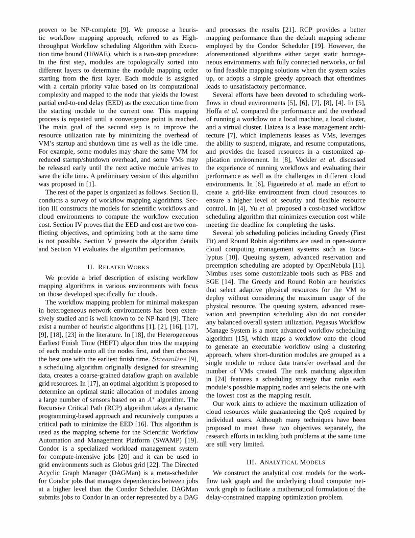
Fig. 1 illustrates an example of three reservation re-quests made on one cloud node during different timeslots. For example, request 1 reserves 60% of the node’scapacity fromt0 to t2; request 2 reserves 20% fromt1 tot4; request 3 reserves 40% fromt3 to t4. The maximalavailable computing power of this node fromt0 to t4 ispvj ,t0,t4 = min(40%, 20%, 80%, 40%). The largest VMinstance that can be allocated onvj from time t1 to tn,namelypVM

vj ,t1,tn, is computed using resources ofpvj ,t1,tn .

The execution time of moduleui on nodevj during timeslot t1 andtn is then computed astvj ,t1(ui) =

zui∗cui

(·)

pV Mvj,t1,tn

,

wherezuidenotes the aggregated complexity-normalized

input data size of moduleui. Similarly, the maximumlink bandwidth alongLvi,vj during time slottm andtn ismin(Bvi,vj ,tm,tn).

B. Workflow Execution Cost

The cost of running a workflow in a cloud is measuredby the sum of the total time, during which VMs arerunning including idle and overhead time, multiplied by

20%

40%

60%

80%

Timet0 t1 t2 t3 t4t0 t1 t2 t3 t4

VM1

(60%)

VM2 (20%)

VM3

(40%)

Server

Capacity

Time

Server

Capacity

100%

Figure 1. Reserved requests on a single cloud node from time point t0to t4.

TABLE I.NOTATIONS USED IN THE ANALYTICAL COST MODELS.

Parameters DefinitionsGwf = (Vwf , Ewf ) the computation workflowN the number of modules in the workflowui the i-th computing moduleei,j the dependency edge from moduleui to uj

wij the data size transferred over dependency edgeei,jzui

the aggregated input data size of moduleui

cui(·) the computational complexity of moduleui

sti the start time of moduleui

eti the end time of moduleui

Gcn = (Vcn, Ecn) the cloud networkK the total number of nodes in the cloudvj the j-th computer nodevs the source nodevd the destination nodepvj

the total computing power of nodevjpV Mvj,t1,tn

the maximal percentage of computing power of VM

on nodevj from t1 to tnLi,j the network link between nodesvi andvjbvi,vj,t1,tn the bandwidth of linkLi,j from t1 to tn

dvi,vjthe minimum link delay of linkLi,j

tstart the time spent on setting up a virtual machinefor the workflow running environment on a node

tshut the time spent on shutting down a virtual machinetvj (ui) the execution time of moduleui

running on nodevjKG the total number of nodes that have been allocated

for the workflowVMvj ,k the k-th VM on thej-th nodeMvj

the total number of VMs on thej-th nodepV Mvj,k

the computing power ofV Mvj,k

the corresponding VM’s capacity. The time spent ondeploying VM on a particular nodevj consists of thefollowing components:

1) The VM startup time for selecting a virtual node andtransferring a virtual image as well as the boot-uptime. It is assumed to be a fixed value oftstart.

2) The running time for every assigned module on thecorresponding VM. Suppose that a setU of mod-ules are assigned onVMvj ,k, and start to run fromtime ts and end at timete in a sequential manner.The running time for these modules is computed as∑

ui∈U zui·cui

(·)

pV Mvj,k

.

3) The idle time between the execution time of anytwo modules. When two modules run on the sameVM, there could be some idle time after one moduleis completed and before the next module starts,calculated asIdle(VMvj ,k) =

∑ui∈U (sti − eti−1).

4) The VM shutdown time, which is also assumed to aconstant oftshut.

Hence, the total resource cost for workflowGwf is:

TC(Gwf) =∑N

i=1 zui· cui

(·)

+∑KG

j=1

∑Mvj

k=1 pVMvj,k· (tstart + Idle(VMvj ,k) + tshut),

(1)whereN is the total number of modules in a workflow,KG

denotes the total number of nodes that have been allocatedfor the workflow, andMvj denotes the total number ofVMs that have been set up on nodevj .

The Utilization Rate (UR) is defined as:

UR =

∑N

i=1 zui· cui

(·)

TC(Gwf), (2)

which measures the efficiency of the cloud resource uti-lization excluding the VM overhead. Obviously, the cloudprovider always desires to maximize this ratio, i.e. reducethe cost to improve the resource utilization rate, whichleads to a higher system throughput. For convenience, weprovide a summary of the notations used in the cost modelsin Table I.

Minimum End-to-end Delay (MED) is an importantperformance requirement in time-critical applications es-pecially for interactive operations. Our mapping objectiveis to select an appropriate set of virtual nodes to set upVM instances for module execution to achieve MED. Theutilization rate can be improved by cutting down the VMstartup, shutdown and idle time. Our approach choosesthe mapping scheme that results in a higher UR underthe same End-to-End Delay (EED) constraint. Once amapping schedule is determined, EED is calculated as thetotal time incurred on the critical path (CP), i.e. the longestexecution path from the source module to the destinationmodule.

IV. PROBLEM FORMULATION

A scheduleS with the maximum resource utilizationrate may be obtained by simply mapping all the modulesonto one node. However, such a scheduleS usually has amuch longer EED than the optimal one.

We first consider a bi-objective scheduling problem tominimize the EED and maximize the utilization rate (orto minimize the total overhead). These two objectives areconflictive and cannot be achieved at the same time, asstated in Theorem 1.

Theorem 1:The bi-objective problem of minimizingthe EED and maximizing the utilization rate is non-approximable within a constant factor.

Proof: We consider a simple instance of the problemthat involves only three modules,u1, u2 andu3, and twocomputing nodes,v1 and v2, whose computing powershave a relationshippv1 = kpv2 . We assume a constant VMstartup timeSA and shutdown timeSU . The computa-tional complexity of modulesu1 andu2 has a relationshipcu1(·) = kcu2(·), and they provide two input datasetsto u3. The link bandwidth between these two nodes isa constantbv1,v2,t = Bv1,v2 without any other transfertask scheduled. The data size transferred fromu2 to u3

is represented byz12 = mBv1,v2 . Assume thatzu1 = zu2

and the data transfer time is small enough to be ignoredcompared with the module running time. Note that datatransfer in cloud environments is fast and such cost istypically not included in the user bill. There exist twofeasible solutions S1 and S2:

(i) S1 is optimal for EED: The modulesu1 and u3

are scheduled on nodev1, and moduleu2 is scheduledon nodev2. Two independent virtual nodes can start upsimultaneously. The EED of S1 is calculated in Eq. 3where cu1(·) = kcu2(·) and pv1 = kpv2 . As u1 and u2

are independent, they can run in parallel on two differentvirtual nodes, and thus only the latest running time needsto be counted for the EED. The efficiency resource (ERC),which is the useful cost for running the workflow (i.e. userpayload), is computed in Eq. 4 . The utilization rate of S1is calculated in Eq. 5.

EED(S1) = SA+cu1(·) · zu1

pv1+

z12

bv1,v2+cu3(·) · zu3

pv1+SU.

(3)

ERC = (k + 1)cu2(·) · zu2 + z12 + cu3(·) · zu3 . (4)

UR(S1) =ERC

ERC + (k + 1)(SA+ SU)pv2. (5)

(ii) S2 is optimal for the utilization rate: All the modulesshould be mapped tov1, which is more powerful, toachieve a better EED with maximized utilization rate. Tocalculate the EED, the running time ofu1 andu2 needsto be computed first. In the beginning, two modules needto share the computing power ofv1 until u2 is finished.The running time foru2 is

2cu2(·)·zu2

pv1=

2cu1(·)·zu1

kpv1

when ui is still in execution. Whenu2 releases thenode, the running time for the remaining portion ofu1

iscu1(·)∗zu1−

cu1(·)∗zu1k

pv1. Thus the EED(S2), ERC’ and

UR(S2) can be calculated as follows:

EED(S2) = SA+cu1(·) · zu1

pv1+

z12

bv1,v2+cu3(·) · zu3

pv1+SU.

(6)

ERC′ = (k + 1)cu2(·) · zu2 + z12 + cu3(·) · zu3 = ERC.

(7)

UR(S2) =ERC

ERC + (SA+ SU) · pv1

=ERC

ERC + k(SA+ SU) · pv2> UR(S1).

(8)

Since the transfer time is much faster than the runningtime, S1 has a smaller EED and also a smaller utilizationrate, which contradicts our assumption on its optimality.Therefore, it is impossible to optimize both objectives atthe same time. Thus, we attempt to maximize the utiliza-tion rate within the constraint of the largest acceptableEED.

We consider the following delay-constrained utilizationmaximization problem for workflow mapping:

Definition 1: Given a DAG-structured computing work-flow Gwf = (Vwf , Ewf ), and an arbitrary computer net-work in a cloud environmentGcn = (Vcn, Ecn) with time-dependent link bandwidth and node computing power, wewish to find a workflow mapping schedule such that theutilization rate is maximized within the largest acceptableend-to-end delay constraint, i.e. the execution time bound(ETB):

maxall possible mappings

(URGcn(Gwf )), such thatEED ≤ ETB.

(9)Here,URGcn

(Gwf ) is the product of the utilization ratesof all the resources that are assigned to either run a moduleor transfer data as shown in Eq. 2. Apparently, a smallernumber of resources yield a higher combined UR.

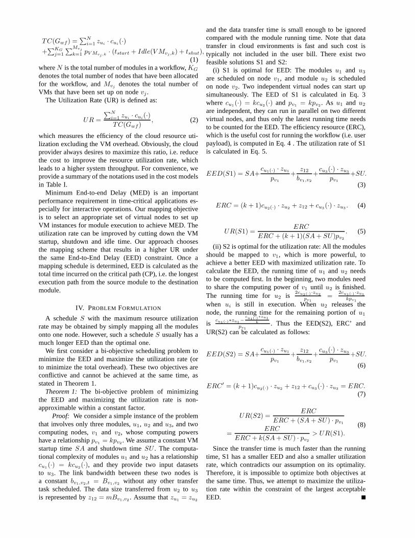
V. A LGORITHM DESIGN

We propose a two-step heuristic workflow mapping ap-proach, referred to as High-throughput Workflow schedul-ing Algorithm with Execution time bound (HiWAE). In thefirst step, modules are divided into different layers throughtopological sorting, which determines the module mappingorder starting from the first layer. Modules are assignedwith different priority values based on a combined con-sideration of their complexities and whether or not theyare on the critical path (CP). Each module is mapped tothe node that results in the lowest partial EED from thestarting module to the current one. This module mappingprocess is repeated until the difference in EED betweentwo contiguous rounds falls below a certain threshold.The second step improves the resource utilization rate bycutting down the VM’s startup, shutdown, and idle time.Strategies used for this purpose include module groupingon the same VM to save the startup/shutdown time andresource release to save the idle time. The pseudocode ofHiWAE is provided in Alg. 1.

Algorithm 1 HiWAE(Gwf , Gcn, ts, ETB)Input: workflow task graphGwf , cloud network graphGcn, workflow’searliest start timets, the execution time bound ETBOutput: a task scheduling scheme with the minimum resource costwithin the given execution time bound1: EEDOrientedForwardMapping(Gwf , Gcn, ts);2: DelayConstraintedBackwardMapping(Gwf , Gcn,Mtm, ts, ETB).

A. Step 1: Minimized End-to-End Delay (MED)

1) Construct a computing environmentGcn∗ with ho-

mogenous computing nodes and communication linksto calculate the initial Critical Path (CP). Sinceour cloud environment supports in-advance resourcereservations in addition to on-demand requests, theavailable resource capacity graph is time dependentand a set of time stamps are used to represent andtrack the periods when resources remain unchanged.

2) Call EEDOrientedForwardMapping() function inAlg. 2 to map all modules to underlying cloud nodes.

Data Center

Layer 1 Layer 2 Layer l-1 Layer l

u1

u3

u2

u4 ul

ut

Layer 3

...

...

uN-1

uN

Recursive Mapping order Module-Node MappingDependency Edge

...

...

Figure 2. Layer-ordered prioritized modules mapped to the underlyingcloud.

We first compute the CP by employing the well-known polynomial-time Longest Path (LP) algorithm,namely FindCriticalPath() , and then run the pri-oritized module mapping algorithmPModulesMap-ping() to map the workflow to the network graphuntil the convergence of EED is reached, as shownin Fig. 2.

Algorithm 2 EEDOrientedForwardMapping(Gwf , Gcn,

ts)Input: workflow task graphGwf , cloud network graphGcn, workflow’searliest start timetsOutput: the temporary mapping scheme with the minimum end-to-enddelay (MED)1: i = 1;2: Gwf

∗ = mapped workflow based onGcn∗;

3: CPi=FindCriticalPath (Gwf∗);

4: call MEDi = PModulesMapping(Gwf , Gcn, ts);5: updateGwf

∗;6: while |MEDi −MEDi−1| ≥ Threshold do7: CPi=FindCriticalPath (Gwf

∗);8: call MEDi =PModulesMapping(Gwf , Gcn, ts);9: updateGwf

∗;10: i++;11: end while12: returnMEDi.

The pseudocode ofPModulesMapping() algorithm isprovided in Alg. 3. This algorithm first conducts topo-logical sorting to sort modules into different layers. Eachmodule is assigned a priority value based on its computingand communication requirements. The module on the CPis given the highest priority value within the same layer.Starting from the first layer, each module is mapped ontoan appropriate node with the lowest partial executiontime from the starting module. A backtracking strategyis adopted to adjust the mapping of the preceding mod-ules (i.e. pre-modules) of each newly mapped module inorder to further reduce its partial EED. The remapping

of any pre-module may also trigger the remapping ofits succeeding modules (i.e. suc-modules) if necessary.Such back-and-forth remapping is only limited to onelayer, i.e. confined within the affected area in order tocontrol the algorithm’s complexity. The shaded modulesthat comprise of the CP are given the highest priority intheir corresponding layers. In Fig. 2, the forward orderto map those modules followsu1, u3, u2, u4, ut, ...,uN−1, uN , as marked by the dotted arrows. A new CP iscomputed after each round of module mapping and suchmapping is repeated until the improvement of EED overthe previous round is below a certain threshold.

The complexity of this iterative module mapping algo-rithm isO(k · l ·N · |Ecn|), wherel is the number of layersin the sorted task graph,N is the number of modules inthe task graph,Ecn is the number of links in the cloudnetwork graph, andk is the number of iterations wherethe obtainedEED meets a certain requirement.

Algorithm 3 PModulesMapping(Gwf, Gcn, ts)

Input: workflow task graphGwf , cloud network graphGcn, workflow’searliest start timetsOutput: the temporary mapping scheme with the best EED namelyMED1: for all uj ∈ CP do2: setuj .flag = 1;3: end for4: conduct topological sorting and assign the priority value to each

module;5: dMinMED = ∞;6: for all ui ∈ SortedArraydo7: for all vj ∈ Node SetVcn do8: calculate the start running time forui run onvj ;9: call GetPartialMED() to calculate the partial EED forui

mapped onvj ;10: if EED in this round is smaller than previous roundthen11: update mapping result for current module;12: end if13: end for14: end for

The above mapping procedure is illustrated in Fig. 2,where the upper part represents a DAG-structured work-flow with shaded modules along the CP, and the lowerpart represents a cloud environment. After the topologicalsorting, u1 falls in layer 1;u2, u3 and u4 fall in layer2. The modules in layer 1 are mapped ontovs first, thenthe modules in layer 2, and so on. For example,ut hasits pre-modules asu3 and u4, which are mapped ontov3 and v2, respectively. The mapping strategy that leadsto the lowest partial EED is chosen for that module. Weassume that the inter-module communication cost withinthe same node is negligible as the data transfer within thesame memory is typically much faster than that across anetwork. Since the resource capacity is time dependentin a cloud environment, instead of calculating one partialEED for each possible mapping, we calculateK (i.e. thenumber of time slots for one cloud node) possible partialEEDs.

After we map the downstream layer, we adjust its up-stream layer’s modules depending on its current mappingresult. For example, in the above case,ut is mapped tovt.We need to adjust its pre-modulesu3 andu4. During the

15%

30%

20%

100%

VM1

(medium)50%

VM2

(large)

Server

Capacity

90%

70%

0 vs1 t1 ve1 STi t2 vs2 t4 ve2 Time

VM3

VM5

VM4

Figure 3. Map moduleui with start running timeSTi on a cloud nodewith three possible VMs instances in forward mapping.

adjustment process, we also need to calculate the partialEED. Instead of calculating the EED from the sourcemodule to the adjusted module, we calculate the partialEED from the source module to its latest finished suc-module.

This module mapping process is essentially a dynamicprogramming process. Let us defineuj ∈ pre(ui) as theset of pre-modules of our current mapping moduleui, andMN(uj) as uj ’s mapping node. We have the followingrecursive Eq. 10 leading to the minimalEED(ui, vk) forthe forward mapping.

Similarly, we defineul ∈ suc(ui) as the set ofui’s suc-modules. We also define a recursive equation to updateEED(ui) as in Eq. 11 for the backward mapping.

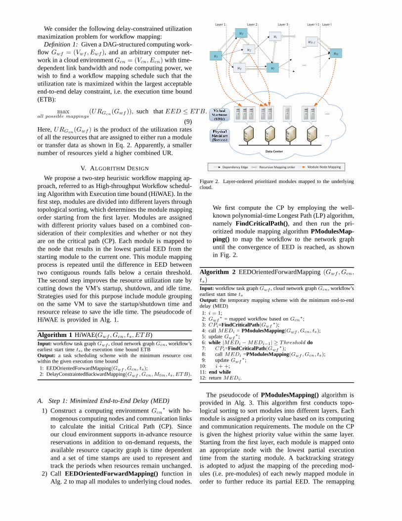
Fig. 3 illustrates how the partial EED is calculated for amodule to be mapped on a cloud node.VM1 andVM2 arevirtual machines that have been deployed to run some pre-modules. We can calculate the execution start time (STi)for moduleui, and then find out the time slot whereSTi

is located. We check all the possible VM strategies, andselect the one with the lowest partial EED. In this example,there are three possible VMs that can be allocated forui,namely,VM3, VM4 andVM5. We calculate the executiontime of ui on VM3 to obtain a partial EED, then check ifthe execution time is shorter than the life time ofVM3. Ifnot, we calculate the execution time onVM4; otherwise,we calculate the execution time onVM5. We comparethe partial EED on each VM, and select the one with thelowest partial EED.

B. Step 2: Reduce VM Overhead

In the second step of this algorithm, we want to reducethe VM overhead for the workflow while still meeting theuser-specified execution time bound (ETB). The overheadsin a cloud include setting up, shutting down and releasinga VM as well as the VM’s idle time. The goal of thisstep is to reduce unnecessary overheads and improve theresource utilization for higher system throughput.

We provide below a brief description ofDelayCon-straintedBackwardMapping(), which is presented in

EED(ui) = minvk∈Vcn

( maxuj∈pre(ui)

(EED(uj ,MN(uj)) +wij

bj,k) +

zui· cui

(·)

pk) (10)

EED(ui) = minvk∈Vcn

( maxuj∈pre(ui)

(EED(uj ,MN(uj))+wij

bj,k)+

zui· C(·)

pk+ max

ul∈suc(ui)(wkMN(ul)

bk,MN(ul)+

zul· cui

(·)

pMN(ul))) (11)

Algorithm 4 DelayConstraintedBackwardMapping(Gwf,

Gcn,Mtm, ts, ETB)Input: workflow task graphGwf , cloud network graphGcn, themapping result from step 1, earliest start timets, execution time boundETB.Output: mapping result with the lowest cost UR withinETB.1: Calculate the maximal acceptable running time for each module i as

MARTi;2: SortedArray = topological and priority sort;3: for all ui ∈ SortedArraydo4: SET findReuse = false;5: for all vj ∈ Node SetVcn do6: if vj has allocated VMthen7: call ReuseVM() to see whether we can reuse a VM onvj

;8: if vj has reusable VMthen9: update mapping result;

10: break;11: end if12: end if13: call AllocateNewVM() to allocate a new VM onvj ;14: end for15: end for

Alg. 4.1) Combine the user-specified execution time bound

(ETB) with the MED calculated from Step 1 to obtainthe initial maximal acceptable running time (MART) foreach module. The running time is calculated asMARTi =RTi ·

ETBMED

.2) Perform topological sorting in a reverse direction

starting from the destination module and assign the cor-responding priority value for each module similar to Step1.

3) For each moduleui from the last module to the firstmodule in the reverse topological sorting list, we comparethe mapping result for each possible mapping node andselect the node and its corresponding VM that incurs thelowest VM overhead as the final mapping node/VM forthis module. There are two cases to consider:i) If the mapping node has some allocated VMs, we then

call ReuseVM() method to check whether or notwe can reuse one of these VMs on that node. Twoconditions must be satisfied when we reuse a module:a) The available VM resource should be sufficient torun the module. b) Any possible idle time should beless than the time to shut down a VM and start upa new one. If both conditions are satisfied and thepartial EED to this module is less than previouslyfound one, we update the mapping information.

ii) If the mapping node has no VMs or those VMs cannot be reused, we callAllocateNewVM() to allocatea new VM for this module. TheAllocateNewVM()

15%

30%

20%

100%

Server

Capacity

80%

70%

0 t1 t2 ETi t3 t4 Time

VM3

VM2

VM1

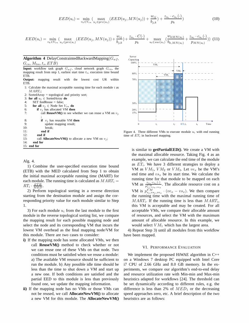
Figure 4. Three different VMs to execute moduleui with end runningtime of ETi in backward mapping.

is similar togetPartialEED(). We create a VM withthe maximal allocable resource. Taking Fig. 4 as anexample, we can calculate the end time of the moduleas ETi. We have 3 different strategies to deploy aVM as VM1, VM2 or VM3. Let vex be the VM’send time andvsx be its start time. We calculate therunning time for that module to be mapped on eachVM as

zui·cui

(·)

pV Mvj,vsx,vex

. The allocable resource cost on a

VM is pV Mvj ,vsx,vex

· (vex − vsx). We then comparethe running time with the maximal running time ofMARTi. If the running time is less thanMARTi,this VM is acceptable and may be created. For allacceptable VMs, we compare their allocable amountof resources, and select the VM with the maximumamount of allocable resource. In this example, wewould selectVM1 which has the largest area.

4) Repeat Step 3) until all modules from this workflowhave been mapped.

VI. PERFORMANCEEVALUATION

We implement the proposed HiWAE algorithm in C++on a Windows 7 desktop PC equipped with Intel Corei7 CPU of 2.66 GHz and 8.0 GB memory. In the ex-periments, we compare our algorithm’s end-to-end delayand resource utilization rate with Min-min and Max-minheuristics adapted for workflows [24]. The threshold canbe set dynamically according to different rules, e.g. thedifference is less than 2% ofMED1 or the decreasingspeed approaches zero, etc. A brief description of the twoheuristics are as follows:

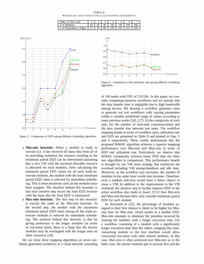
TABLE II.WORKFLOW CASES USED IN THE CLOUD MAPPING EXPERIMENTS.

Index of Test Case 1 2 3 4 5 6 7# of Modules 10 20 40 60 80 100 200# of Dependency Edges 21 36 88 120 156 215 420

Testcase

EED(hr)

1 2 3 4 5 6 70.5

1.0

1.5

2.0

2.5

3.0

3.5

HiWAE

Min-min

Max-min

ETB

Figure 5. Comparison of EED among different scheduling algorithms.

• Min-min heuristic: When a module is ready toexecute (i.e. it has received all input data from all ofits preceding modules), the resource resulting in theminimum partial EED can be determined (assumingthat a new VM with the maximal allocable resourceis allocated for each module). After calculating theminimum partial EED values for all such ready-to-execute modules, the module with the least minimumpartial EED value is selected for immediate schedul-ing. This is done iteratively until all the modules havebeen mapped. The intuition behind this heuristic isthat each iterative step incurs the least EED increasewith the hope that the final EED is minimized.

• Max-min heuristic: The first step of this heuristicis exactly the same as the Min-min heuristic. Inthe second step, the module with the maximumminimum partial EED value among all the ready-to-execute modules is selected for immediate schedul-ing. The intuition behind this heuristic is that bygiving preference to the longer modules (in termsof execution time), there is a hope that the shortermodules may be overlapped with the longer ones onother resources [24].

We run these three mapping algorithms on seven ran-domly generated workflows in a cloud network consisting

Testcase

UR

1 2 3 4 5 6 70.5

0.6

0.7

0.8

0.9

1.0

HiWAE

Min-minMax-min

Figure 6. Comparison of the utilization rate among different schedulingalgorithms.

of 100 nodes with CPU of 2.0 GHz. In this paper, we con-sider computing-intensive workflows and we assume thatthe data transfer time is negligible due to high bandwidthamong servers. We develop a workflow generator classto generate our test workflows with varying parameterswithin a suitably predefined range of values according tosome previous works [26], [27]: (i) the complexity of eachtask; (ii) the number of inter-task communications andthe data transfer size between two tasks. The workflowmapping results in terms of workflow sizes, utilization rateand EED are presented in Table II and plotted in Figs. 5and 6 respectively. These results demonstrate that theproposed HiWAE algorithm achieves a superior mappingperformance over Min-min and Max-min in terms ofEED and utilization rate. Particularly, we observe thatHiWAE consistently achieves lower EED than the othertwo algorithms in comparison. This performance benefitis brought by our VM reuse strategy that minimizes theoverhead including VM startup/shutdown and idle time.Moreover, as the workflow size increases, the number ofmodules in the same layer would also increase. Therefore,even a random selection would have a better chance toreuse a VM. In addition to the improvement in the VMoverhead, the iterative step to further improve EED of theentire workflow also leads to lowerEED than Min-minand Max-min because they only consider minimum partialEED for each module.

As discussed in [25], the percentage of modules as-signed to their first choices is likely to be higher for Min-min than for Max-min, which results in a smaller EED.Max-min attempts to minimize the penalties incurred byrunning the modules with a longer execution time. Fora workflow consisting of a module with a significantlylonger execution time than the others, mapping this time-consuming module to the best machine would allowconcurrent execution with other shorter modules. In thiscase, Max-min is often preferred over Min-min as in thelatter case, the shorter modules get to execute first and the

longest modules get executed with many idle nodes forlower utilization rate. Thus, Max-min results in a morebalanced workload across the nodes and a better EED.

Min-min and Max-min achieve similar utilization ratesbecause they are more likely to choose the same resourcefor each module (as stated in the first step of Min-min andMax-min heuristics). Our algorithm achieves about 24% -30% higher resource utilization than Min-min and Max-min on average because of our VM reuse strategy thatminimizes the overhead.

These experimental results show that the proposed Hi-WAE algorithm exhibits a better control over the executiontime of a workflow compared to Min-min and Max-min heuristics, and yields a significantly higher resourceutilization rate by reducing the VM overhead during theworkflow execution.

VII. C ONCLUSION AND FUTURE WORK

Many big data sciences are starting to use clouds asthe major computing platform. We formulated a workflowscheduling problem in cloud environments. In general, itis of the cloud service provider’s interest to improve thesystem throughout to satisfy as many user requests aspossible using the same hardware resources. Hence, theresource utilization rate is a very important performancemetric, which, however, has not been sufficiently ad-dressed by many existing workflow scheduling algorithmsdeveloped for clouds. Also, from the user’s perspective,one primary goal is to minimize the execution time ofeach individual workflow as stated in certain Quality ofService requirement.

Our mapping algorithm aims to achieve the dual goalsof end-to-end delay performance and low overhead usinga two-step approach. In the first step, modules are topo-logically sorted and mapped layer-by-layer to identify thebest mapping strategy with the minimal execution time. Ifthe final finish time is earlier than the latest finish timespecified by the user, the extra allowed time delay is usedto relax the mapping of modules to reduce the cost on VMsetup and shutdown as well as the idle time. A backwardmodule remapping procedure from the last layer towardthe first layer is conducted to cut down the overhead.One strategy is to maximize the allocable volume of aVM to open the window for more modules to reuse it.After this backward mapping, any unused VM volume interms of extra time is not requested. The simulation re-sults demonstrated that our algorithm significantly reducesthe VM cost compared with other representative cloudscheduling algorithms with a comparable or lower totalexecution time. It is of our future interest to implement andtest this scheduling algorithm in local cloud testbeds andproduction cloud environments to support real-life large-scale scientific workflows.

ACKNOWLEDGEMENT

We would like to acknowledge Ms. Yang Zhao for hercontributions to the preliminary design and implementa-tion of the workflow scheduling algorithm proposed in theconference paper [1].

REFERENCES

[1] M. Zhu, Q. Wu and Y. Zhao. A Cost-effective SchedulingAlgorithm for Scientific Workflows in Clouds. InProc. ofthe 31st IEEE International Performance Computing andCOmmunication Conference (IPCCC), pp. 256-265, 2012.

[2] A. Bala and I. Chana. A Survey of Various WorkflowScheduling Algorithms in Cloud Environment. InProc. ofthe 2nd National Conference on Information and Communi-cation Technology, pp. 26-30, 2011.

[3] S. Zhang, X. Chen, and X. Huo. Cloud Computing Researchand Development Trend. InProc. of the 2nd InternationalConference on Future Networks(ICFN’10), pp. 93-97, 2010.

[4] J. Yu, R. Buyya, and C.K. Tham. Cost-based Schedulingof Scientific Workflow Applications on Utility Grids. InProc. of the 1st IEEE International Conference on e-Scienceand Grid Computing(e-Science 2005), Dec. 5-8, 2005,Melbourne, Australia.

[5] C. Hoffa, G. Mehta, T. Freeman, E. Deelman, K. Keahey, B.Berriman, and J. Goo. On the Use of Cloud Computing forScientific Workflows. InProc. of the IEEE 4th InternationalConference on eScience, pp. 640-645, 2008.

[6] R. J. Figueiredo, P. A. Dinda, and J. A.B. Fortes.A Casefor Grid Computing On Virtual Machines. In Proc. ofDistributed Computing Systems, pp. 550-559, 2003.

[7] B. Sotomayor, K. Keahey, and I. Foster. Combining batchexecution and leasing using virtual machines. InProc. ofthe 17th International Symposium on High PerformanceDistributed Computing(HPDC’08), Boston, Massachusetts,USA, June 23-27, 2008.

[8] J. Vockler, G. Juve, E. Deelman, M. Rynge, and B. Berriman.Experiences using cloud computing for a scientific workflowapplication. InProc. of the 2nd International Workshop onScientific Cloud Computing(ScienceCloud’11), pp. 15-24,2011.

[9] B. Agarwalla, N. Ahmed, D. Hilley, and U. Ramachandran.Streamline: a scheduling heuristic for streaming applicationon the grid. InProc. of the 13th Multimedia Computing andNetworking Conf., San Jose, CA, 2006.

[10] D. Nurmi, R. Wolski, C. Grzegorczyk, G. Obertelli, S.So-man, L. Youseff, and D. Zagorodnov.The Eucalyptusopen-source cloud-computing system. InProc. of IEEEInternational Symposium on Cluster Computing and the Grid(CCGrid’09), 2009.

[11] Open Nebular, http://www.opennebula.org.[12] Amazon EC2, http://aws.amazon.com/ec2/.[13] Google App Engine, https://developers.google.com/app- en-

gine/.[14] Nimbus, http://nimbusproject.org..[15] E. Deelman, G. Singh, M. H. Su, J. blythe, and Y. e.a.

Gil. Pegasus: A framework for mapping complex scientificworkflows onto distributed systems.Scientific ProgrammingJournal, vol. 13, pp. 219-237, July 2005.

[16] Q. Wu and Y. Gu. Supporting distributed application work-flows in heterogeneous computing environments. InProc. ofthe 14th IEEE Int. Conf. on Parallel and Distributed Systems,Melbourne, Australia, pp. 3-10, 2008.

[17] A. Sekhar, B. Manoj, and C. Murthy. A state-space searchapproach for optimizing reliability and cost of execution indistributed sensor networks. InProc. of Int. Workshop onDistributed Computing, pp. 63-74, 2005.

[18] S. Topcuoglu and M. Wu. Task scheduling algorithmsfor heterogeneous processors. InProc. of the 8th IEEEHeterogeneous Computing Workshop(HCW’99), pp. 3-14,1999.

[19] Q. Wu, M. Zhu, X. Lu, P. Brown, Y. Lin, Y. Gu, F. Cao,and M. Reuter. Automation and management of scientificworkflows in distributed network environments. InProc. ofthe 6th Int. Workshop on Sys. Man. Tech., pp. 1-8, 2010.

[20] Condor,http://www.cs.wisc.edu/condor.

[21] DagMan,http://www.cs.wisc.edu/condor/dagman.[22] Globus,http://www.globus.org.[23] T. Ma and R. Buyya. Critical-path and priority based

algorithms for scheduling workflows with parameter sweeptasks on global grids. InProc. of the 17th Int. Symp. onComputer Architecture on High Performance Computing, pp.251-258, 2005.

[24] A. Mandal, K. Kennedy, C. Koelbel, G. Marin, J. Mellor-Crummey, B. Liu, and L. Johnsson. Scheduling Strategiesfor Mapping Application WorMows onto the Grid. InProc.of the IEEE International Symposium on High PerformanceDistributed Computing(HPDC), pp. 125-134, 2005.

[25] T. D. Braun, H. J. Siegel, and N. Beck. A comparison ofeleven static heuristics for mapping a class of independenttasks onto heterogeneous distributed computing systems. InJournal of Parallel and Distributed computing, 61(6): 810-837, 2011.

[26] Q. Wu, M. Zhu, Y. Gu, P. Brown, X. Lu, W. Lin, andY. Liu. A Distributed Workflow Management System withCase Study of Real-life Scientific Applications on Grids.InJournal of Grid Computing, vol. 10(3), pp. 367-393, 2012.

[27] Q. Wu, Y. Gu, Y. Lin, and N. Ra. Latency Modelingand Minimization for Large-scale ScientificWorkflows inDistributed Network Environments. Inthe 44th Annual Sim-ulation Symposium (ANSS 2011), 2011, pp. 205-212.

!

Michelle M. Zhu received the Ph.D. degreein computer science from Louisiana State Uni-versity in 2005. She spent two years in theComputer Science and Mathematics Division atOak Ridge National Laboratory for her Ph.D.dissertation from 2003 to 2005. She is currentlyan associate professor in the Computer Sci-ence Department at Southern Illinois Univer-sity, Carbondale. Her research interests includedistributed and high-performance computing,remote visualization, bioinformatics, and sensor

networks.

Fei Cao received the B.S. degree in soft-ware engineering from Zhejiang University,P.R. China, in 2007, the M.S. degree in com-puter science from California State University,Fullerton, in 2009. She is currently a Ph.D.student in the Department of Computer Scienceat Southern Illinois University, Carbondale. Herresearch interests include distributed computingand high-performance computing.

Chase Q. Wu received the B.S. degree inremote sensing from Zhejiang University, P.R.China, in 1995, the M.S. degree in geomaticsfrom Purdue University in 2000, and the Ph.D.degree in computer science from LouisianaState University in 2003. He was a researchfellow in the Computer Science and Mathemat-ics Division at Oak Ridge National Laboratoryduring 2003-2006. He is currently an AssociateProfessor with the Department of ComputerScience at University of Memphis. His research

interests include parallel and distributed computing, computer networks,and cyber security.