UNIVERSITY OF CALIFORNIARIVERSIDE

Higher Symplectic Geometry

A Dissertation submitted in partial satisfactionof the requirements for the degree of

Doctor of Philosophy

in

Mathematics

by

Christopher Lee Rogers

June 2011

Dissertation Committee:

Professor John C. Baez, ChairpersonProfessor Julia BergnerProfessor Yat-Sun Poon

Copyright byChristopher Lee Rogers

2011

The Dissertation of Christopher Lee Rogers is approved:

Committee Chairperson

University of California, Riverside

Acknowledgments

I wish to thank my advisor John Baez for his encouragement and guidance in completing

this thesis. I would also like to thank Julie Bergner and Yat-Sun Poon for serving on

my committee.

I wish to acknowledge the following individuals for helpful discussions, com-

ments, and suggestions: Maarten Bergvelt, Henrique Bursztyn, Jim Dolan, Vasily Dol-

gushev, Yael Fregier, Alex Hoffnung, Allen Knutson, Dmitry Roytenberg, Urs Schreiber,

Jim Stasheff, Danny Stevenson, Thomas Strobl, Alan Weinstein, and Marco Zambon.

Part of this work was completed while I was a Junior Research Fellow at the

Erwin Schrodinger International Institute for Mathematical Physics. I thank them for

their hospitality and financial support. Additional support for this work was provided

by NSF grants PHY-0653646 and DMS-0856196, and FQXi grant RFP2-08-04.

iv

ABSTRACT OF THE DISSERTATION

Higher Symplectic Geometry

by

Christopher Lee Rogers

Doctor of Philosophy, Graduate Program in MathematicsUniversity of California, Riverside, June 2011

Professor John C. Baez, Chairperson

In higher symplectic geometry, we consider generalizations of symplectic man-

ifolds called n-plectic manifolds. We say a manifold is n-plectic if it is equipped with

a closed, nondegenerate form of degree (n + 1). We show that certain higher algebraic

and geometric structures naturally arise on these manifolds. These structures can be

understood as the categorified or homotopy analogues of important structures studied

in symplectic geometry and geometric quantization. Our results imply that higher sym-

plectic geometry is closely related to several areas of current interest including string

theory, loop groups, and generalized geometry.

We begin by showing that, just as a symplectic manifold gives a Poisson algebra

of functions, any n-plectic manifold gives a Lie n-algebra containing certain differential

forms which we call Hamiltonian. Lie n-algebras are examples of strongly homotopy

Lie algebras. They consist of an n-term chain complex equipped with a collection of

skew-symmetric multi-brackets that satisfy a generalized Jacobi identity.

We then develop the machinery necessary to geometrically quantize n-plectic

manifolds. In particular, just as a prequantized symplectic manifold is equipped with

a principal U(1)-bundle with connection, we show that a prequantized 2-plectic mani-

fold is equipped with a U(1)-gerbe with 2-connection. A gerbe is a categorified sheaf,

or stack, which generalizes the notion of a principal bundle. Furthermore, over any 2-

plectic manifold there is a vector bundle equipped with extra structure called a Courant

algebroid. This bundle is the 2-plectic analogue of the Atiyah algebroid over a prequan-

tized symplectic manifold. Its space of global sections also forms a Lie 2-algebra. We

use this Lie 2-algebra to prequantize the Lie 2-algebra of Hamiltonian forms.

Finally, we introduce the 2-plectic analogue of the Bohr-Sommerfeld variety

associated to a real polarization, and use this to geometrically quantize 2-plectic man-

v

ifolds. For symplectic manifolds, the output from quantization is a Hilbert space of

quantum states. Similarly, quantizing a 2-plectic manifold gives a category of quantum

states. We consider a particular example in which the objects of this category can be

identified with representations of the Lie group SU(2).

vi

Contents

1 Introduction 1

2 n-Plectic geometry 132.1 Linear theory . . . . . . . . . . . . . . . . . . . . . . . . . . . . . . . . . 132.2 n-Plectic manifolds . . . . . . . . . . . . . . . . . . . . . . . . . . . . . . 152.3 k-Lagrangian submanifolds and k-polarizations . . . . . . . . . . . . . . 18

3 Algebraic structures on n-plectic manifolds 193.1 Hamiltonian forms . . . . . . . . . . . . . . . . . . . . . . . . . . . . . . 213.2 L∞-algebras and Lie n-algebras . . . . . . . . . . . . . . . . . . . . . . . 25

3.2.1 Lie 2-algebras . . . . . . . . . . . . . . . . . . . . . . . . . . . . . 273.3 Lie n-algebras from n-plectic manifolds . . . . . . . . . . . . . . . . . . . 28

4 Lie 2-algebras from compact simple Lie groups 364.1 Group actions on n-plectic manifolds . . . . . . . . . . . . . . . . . . . . 374.2 Compact simple Lie groups as 2-plectic manifolds . . . . . . . . . . . . . 384.3 The string Lie 2-algebra . . . . . . . . . . . . . . . . . . . . . . . . . . . 41

5 Stacks, gerbes, and Deligne cohomology 445.1 Stacks . . . . . . . . . . . . . . . . . . . . . . . . . . . . . . . . . . . . . 455.2 Gerbes . . . . . . . . . . . . . . . . . . . . . . . . . . . . . . . . . . . . . 495.3 Deligne cohomology . . . . . . . . . . . . . . . . . . . . . . . . . . . . . 535.4 2-Connections on U(1)-gerbes . . . . . . . . . . . . . . . . . . . . . . . . 625.5 2-Line stacks . . . . . . . . . . . . . . . . . . . . . . . . . . . . . . . . . 655.6 Holonomy of Deligne classes . . . . . . . . . . . . . . . . . . . . . . . . . 70

6 Prequantization of 2-plectic manifolds 756.1 Overview of prequantization . . . . . . . . . . . . . . . . . . . . . . . . . 756.2 Prequantization of symplectic manifolds . . . . . . . . . . . . . . . . . . 796.3 Courant algebroids . . . . . . . . . . . . . . . . . . . . . . . . . . . . . . 846.4 Courant algebroids and 2-plectic geometry . . . . . . . . . . . . . . . . . 876.5 Central extensions of Lie 2-algebras . . . . . . . . . . . . . . . . . . . . . 97

7 Geometric quantization of 2-plectic manifolds 1047.1 Geometric quantization of symplectic manifolds . . . . . . . . . . . . . . 106

7.1.1 The Bohr-Sommerfeld variety . . . . . . . . . . . . . . . . . . . . 1067.1.2 Example: R2 \ 0 . . . . . . . . . . . . . . . . . . . . . . . . . . 108

7.2 Categorified geometric quantization . . . . . . . . . . . . . . . . . . . . . 109

vii

7.2.1 Example: R3 \ 0 . . . . . . . . . . . . . . . . . . . . . . . . . . 1117.3 Applications to representation theory . . . . . . . . . . . . . . . . . . . . 117

8 Summary and future work 121

Bibliography 128

A Other algebraic structures on n-plectic manifolds 133A.1 dg Leibniz algebras . . . . . . . . . . . . . . . . . . . . . . . . . . . . . . 133A.2 Weak Lie 2-algebras . . . . . . . . . . . . . . . . . . . . . . . . . . . . . 136

B Twisted bundles and the proof of Proposition 5.28 142

viii

Chapter 1

Introduction

Higher symplectic geometry is a generalization of symplectic geometry which

begins with considering manifolds equipped with a closed nondegenerate form of higher

degree. This thesis explains how such a differential form gives rise to algebraic and

geometric structures which act as the higher analogues of important structures found

in symplectic geometry and geometric quantization. Indeed, a recurring theme in this

work is the idea that basic results in symplectic geometry are specific instances of more

general theorems which hold for a much larger class of structures.

In particular, we focus on manifolds equipped with a closed nondegenerate 3-

form. We call such manifolds ‘2-plectic’. In this case, we see that higher symplectic

geometry is intimately related to string theory. We use ideas from higher category

theory and homotopical algebra to develop a geometric quantization procedure for 2-

plectic manifolds. In doing so, we encounter structures known to play important roles in

other string-inspired areas of current interest. These include the theory of L∞-algebras,

loop groups, gerbes, and generalized geometry. Our results shine new light on these

structures, and suggest new relationships among the above fields. We invite the reader

who has some familiarity with these ideas to skip ahead and browse Table 1.1. There we

list examples of such structures and the roles they play in the quantization of 2-plectic

manifolds.

We wish to provide in this introductory chapter a gentle overview of the basic

ideas behind higher symplectic geometry, and describe, with some detail, the main

results of this thesis. We begin with a brief survey of symplectic geometry and geometric

quantization which emphasizes the role played by classical and quantum mechanics.

Higher symplectic geometry is then introduced as a consequence of combining two known

approaches to studying classical field theory: multisymplectic geometry and higher gauge

theory. We conclude by providing a chapter-by-chapter summary of our main results.

1

Symplectic geometry and geometric quantization

Symplectic geometry is the study of manifolds equipped with a closed non-

degenerate 2-form. nondegeneracy, in this context, means that the 2-form gives an

isomorphism between the space of tangent vectors and the space of 1-forms by contrac-

tion or “lowering indices”. Such a 2-form produces a variety of interesting algebraic and

geometric structures. Symplectic manifolds appear in many branches of mathematics

and these structures often provide useful characterizations of important phenomena. In

particular, symplectic manifolds play a crucial role in classical mechanics and represen-

tation theory.

The origins of symplectic geometry, in fact, lie in classical mechanics. In clas-

sical mechanics, one studies the physics of a system of point-like particles. For many

systems of interest, the state of the system at any time is uniquely determined by spec-

ifying the position and momentum of each particle. This state can be interpreted as a

point in a manifold called the ‘phase space’ of the system. The time evolution of the

system is therefore represented by a smooth path in this manifold, which is a solution

to an ordinary differential equation called ‘Hamilton’s equation’. Physical observables

of the system are smooth functions on the manifold. Measurement of an observable

corresponds to evaluating the function at a particular a point of phase space. Remark-

ably, the structures needed to guarantee a solution to Hamilton’s equation, and also

to describe how measurements change in time, are provided by equipping the manifold

with a symplectic 2-form.

For example, the nondegeneracy of the symplectic 2-form guarantees that

Hamilton’s equations have, at least for some interval of time, a solution. More in-

terestingly, the symplectic structure makes the space of functions on the manifold into a

special kind of Lie algebra called a Poisson algebra. The fact that the symplectic 2-form

is closed implies that the corresponding bracket satisfies the Jacobi identity. This Lie

bracket is used to compute the time evolution of observables.

There are many systems of interest, however, which must be studied by using

quantum mechanics, instead of classical mechanics. In these cases, classical mechanics

can be understood as a very rough approximation to the true physical behavior of the

system. In their attempts to understand such quantum systems, physicists developed a

process called ‘quantization’ in which one first considers a system classically, and then

replaces these structures with their quantum analogues. Roughly speaking, in quantum

mechanics the states of the system no longer correspond to points on a manifold, but

rather to vectors in a Hilbert space. Observables no longer correspond to functions on

2

a manifold, but rather to linear operators on the Hilbert space. The time evolution of

a system is given by a solution to a partial differential equation called ‘Schrodinger’s

equation’, rather than Hamilton’s equation. The time evolution of observables is now

determined by the commutator bracket of operators, rather than the Poisson bracket of

functions.

Hence, within the context of symplectic geometry, the physicists’ findings sug-

gests that quantization is a procedure which involves assigning to a symplectic manifold

a Hilbert space, and to the Poisson algebra a representation as linear operators on this

space. This is, in fact, the first step of a rigorous procedure called ‘geometric quanti-

zation’ developed by Kirillov [34], Kostant [37], and Souriau [64] (KKS) in the 1960’s.

It is based on the following facts: If a symplectic 2-form satisfies a certain integrality

condition, then it must be the curvature of a principal U(1)-bundle equipped with a

connection living over the manifold. Such a symplectic manifold is called ‘prequanti-

zable’. Certain global sections of the associated Hermitian line bundle form a Hilbert

space whose inner product is given by the symplectic structure. The connection on the

bundle then determines a faithful representation of the Poisson algebra as operators on

this prequantum Hilbert space.

However, in practice, this Hilbert space is “too large”. The second step in

the KKS procedure involves choosing an additional structure on the manifold called a

‘polarization’. Roughly speaking, a polarization on a symplectic manifold is a special

kind of integrable distribution [63, 70]. The size of the Hilbert space is reduced by

considering only those sections that are covariantly constant in the directions given by

vectors contained in the distribution. This smaller space is called the ‘quantum Hilbert

space’, or ‘space of quantum states’.

Geometric quantization may appear, at first sight, to be a rather mysterious

procedure with limited applicability. Not every symplectic manifold is prequantizable,

and not every prequantized symplectic manifold admits a polarization. Even when such

structures do exist, there are several non-canonical choices to be made. Furthermore, the

presence of certain topological obstructions often implies that additional fine-tuning is

required. Regardless, the KKS procedure is very powerful and has led to a large number

of important results, for example, in the representation theory of Lie groups. Here, one

typically studies the symmetry group of a geometric object by first understanding the

algebraic representation theory of the group. Kirillov and Kostant’s original motivation

for developing geometric quantization was, in some sense, the converse: to construct the

representations of groups as geometric objects. Indeed, the central tenet of Kirillov’s

orbit method [34] is, roughly, that an irreducible representation of a Lie group corre-

3

sponds to a particular symplectic manifold equipped with an action of the group. The

representation itself is recovered as the quantum Hilbert space obtained from geometric

quantization.

Higher degree, higher dimension, and higher structure

After digesting all of this, the curious reader might ask a simple question: What

is so special about 2-forms? After all, many manifolds admit interesting closed forms of

higher degrees, and some of these, such as volume forms, are “nondegenerate”. It is also

reasonable to ask how much, if any, of the above story involving symplectic geometry

and quantization carries over to manifolds equipped with such forms. The main goal of

this thesis is to address these questions.

At its most basic level, higher symplectic geometry involves studying manifolds

equipped with a closed, nondegenerate form of higher degree. We call such a manifold

‘n-plectic’ if the form has degree (n + 1), so that a 1-plectic manifold is a symplectic

manifold. Here, nondegeneracy means that the n-plectic form injectively maps the space

of tangent vectors into the space of n-forms, again by contraction. In contrast with the

symplectic case, this injection is not necessarily an isomorphism. Many examples of

n-plectic manifolds appear “in nature”. These include orientable manifolds, exterior

powers of cotangent bundles, and compact simple Lie groups.

Usually, n-plectic manifolds go by the name of multisymplectic manifolds [16].

Just as symplectic geometry has its origins in the classical mechanics of particles, mul-

tisymplectic geometry was initially developed to study higher-dimensional classical field

theories. Let us briefly explain what this means. As previously mentioned, the time evo-

lution of a point-like particle is described by a path which depends on one variable: time.

So, the ‘world-line’ of a zero-dimensional object is determined by a map from a one-

dimensional manifold. A physicist might call classical mechanics a (0 + 1)-dimensional

field theory. However, describing the behavior of a higher-dimensional object, such as

a string, requires more variables. The amplitude of a vibrating string depends on both

time and the position along the string. Hence, the time evolution of the one-dimensional

string is described by a map from a 2-dimensional manifold or ‘world-sheet’. In this way,

string theory is a (1 + 1)-dimensional field theory. In general, the physics of a (n− 1)-

dimensional object, or ‘brane’, is described by a n-dimensional field theory.

The basic ideas in multisymplectic geometry can be found in Weyl’s 1935 work

on the calculus of variations [68]. It was further developed in the 1970’s mainly by the

Polish school of mathematical physics. The work of Kijowski [32], Tulczyjew [33], and

4

others [51] showed that, just as symplectic manifolds can by used as phase spaces for

(0+1)-dimensional field theories, multisymplectic manifolds can be used as ‘multiphase’

spaces for higher-dimensional field theories. Specifically, the multiphase space used to

describe the physics of an (n−1)-dimensional object is an n-plectic manifold. A solution

to a partial differential equation called the de Donder-Weyl equation corresponds to a

particular n-dimensional submanifold of this space. The data encoded by these subman-

ifolds include the value of the field as well as the value of its ‘multi-momentum’ at each

point in space and time. The multi-momentum is a quantity that is related to the time

and spatial derivatives of the field, in a manner similar to the relationship between the

velocity of a point particle and its momentum. This formalism has several attractive

mathematical features, but it still needs further development before it can replace more

common frameworks used by physicists to study field theories.

The work of Baez and Schreiber [7], Freed [20], Schreiber [60], Sati, Schreiber,

and Stasheff [56] suggests that structures found in classical mechanics can be generalized

by using higher category and homotopy theory and then applied to the study of higher-

dimensional field theories. So far this viewpoint has been most fruitful in studying the

string and brane-theoretic generalizations of gauge theory. Although the details are

quite technical, the basic philosophy behind higher gauge theory is very simple. While

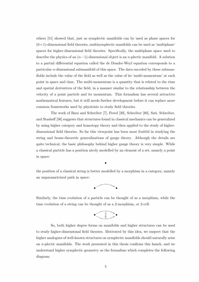
a classical particle has a position nicely modelled by an element of a set, namely a point

in space:

•

the position of a classical string is better modelled by a morphism in a category, namely

an unparametrized path in space:

• %% •

Similarly, the time evolution of a particle can be thought of as a morphism, while the

time evolution of a string can be thought of as a 2-morphism, or 2-cell:

• %%99•

So, both higher degree forms on manifolds and higher structures can be used

to study higher-dimensional field theories. Motivated by this idea, we suspect that the

higher analogues of well-known structures on symplectic manifolds should naturally arise

on n-plectic manifolds. The work presented in this thesis confirms this hunch, and we

understand higher symplectic geometry as the formalism which completes the following

diagram:

5

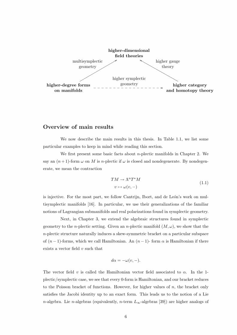
higher-dimensionalfield theories

higher-degree formson manifolds

multisymplecticgeometry

88rrrrrrrrrrrrrrrrrrrrrr higher symplecticgeometry

//__________________ higher categoryand homotopy theory

higher gaugetheory

ffMMMMMMMMMMMMMMMMMMMMMMM

Overview of main results

We now describe the main results in this thesis. In Table 1.1, we list some

particular examples to keep in mind while reading this section.

We first present some basic facts about n-plectic manifolds in Chapter 2. We

say an (n+ 1)-form ω on M is n-plectic if ω is closed and nondegenerate. By nondegen-

erate, we mean the contraction

TM → ΛnT ∗M

v 7→ ω(v,−)(1.1)

is injective. For the most part, we follow Cantrijn, Ibort, and de Leon’s work on mul-

tisymplectic manifolds [16]. In particular, we use their generalizations of the familiar

notions of Lagrangian submanifolds and real polarizations found in symplectic geometry.

Next, in Chapter 3, we extend the algebraic structures found in symplectic

geometry to the n-plectic setting. Given an n-plectic manifold (M,ω), we show that the

n-plectic structure naturally induces a skew-symmetric bracket on a particular subspace

of (n− 1)-forms, which we call Hamiltonian. An (n− 1)- form α is Hamiltonian if there

exists a vector field v such that

dα = −ω(v,−).

The vector field v is called the Hamiltonian vector field associated to α. In the 1-

plectic/symplectic case, we see that every 0-form is Hamiltonian, and our bracket reduces

to the Poisson bracket of functions. However, for higher values of n, the bracket only

satisfies the Jacobi identity up to an exact form. This leads us to the notion of a Lie

n-algebra. Lie n-algebras (equivalently, n-term L∞-algebras [39]) are higher analogs of

6

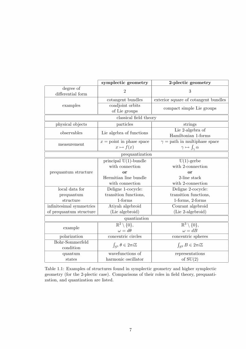
symplectic geometry 2-plectic geometrydegree of

2 3differential form

examplescotangent bundles exterior square of cotangent bundlescoadjoint orbits

compact simple Lie groupsof Lie groups

classical field theoryphysical objects particles strings

observables Lie algebra of functionsLie 2-algebra of

Hamiltonian 1-forms

measurementx = point in phase space γ = path in multiphase space

x 7→ f(x) γ 7→∫γ α

prequantization

prequantum structure

principal U(1)-bundle U(1)-gerbewith connection with 2-connection

or orHermitian line bundle 2-line stack

with connection with 2-connectionlocal data for Deligne 1-cocycle: Deligne 2-cocycle:prequantum transition functions, transition functions,

structure 1-forms 1-forms, 2-formsinfinitesimal symmetries Atiyah algebroid Courant algebroidof prequantum structure (Lie algebroid) (Lie 2-algebroid)

quantization

exampleR2 \ 0, R3 \ 0,ω = dθ ω = dB

polarization concentric circles concentric spheresBohr-Sommerfeld ∫

S1 θ ∈ 2πiZ∫S2 B ∈ 2πiZ

conditionquantum wavefunctions of representations

states harmonic oscillator of SU(2)

Table 1.1: Examples of structures found in symplectic geometry and higher symplecticgeometry (for the 2-plectic case). Comparisons of their roles in field theory, prequanti-zation, and quantization are listed.

7

differential graded Lie algebras. They consist of a graded vector space concentrated

in degrees 0, . . . , n − 1, and are equipped with a collection of skew-symmetric k-ary

brackets, for 1 ≤ k ≤ n + 1, that satisfy a generalized Jacobi identity. In particular,

the k = 2 bilinear bracket behaves like a Lie bracket that only satisfies the ordinary

Jacobi identity up to higher coherent chain homotopy. In Theorem 3.14, we prove that,

given an n-plectic manifold, one can explicitly construct a Lie n-algebra on a complex

consisting of Hamiltonian (n − 1)-forms and arbitrary p-forms for 0 ≤ p ≤ n − 2. The

bilinear bracket, as well as all higher k-ary brackets, are completely determined by the

n-plectic structure.

We consider an important example of this construction in Chapter 4: the Lie 2-

algebra arising from a compact simple Lie group. Every such Lie group has a 1-parameter

family of canonical 2-plectic structures generated by the ‘Cartan 3-form’. These 3-forms

are used to build central extensions of, and line bundles on, the corresponding loop

group [47]. They also play a key role in the theory of gerbes on Lie groups [43] and the

quantization of conjugacy classes [46]. We show how the Lie 2-algebra of Hamiltonian

1-forms on a compact simple Lie group G relates to the ‘string Lie 2-algebra’ of G [4].

It is known that the string Lie 2-algebra can be integrated to a ‘Lie 2-group’ [28]. This

Lie 2-group can be geometrically realized as a topological group which appears in the

study of spin structures on loop spaces.

Since geometric quantization has seen so much success in symplectic geometry,

we wish to extend it to the n-plectic setting. In symplectic geometry, prequantization

involves equipping the manifold with a principal U(1)-bundle with a connection, whose

curvature is the symplectic 2-form. Therefore, in Chapter 5 we consider ‘stacks’, the

2-plectic analogue of bundles. A stack on a manifold can be thought of as a categorified

sheaf i.e. an assignment of a category to each open neighborhood of the manifold. In

particular, the higher analogue of a principal U(1)-bundle is a special kind of stack

called a ‘U(1)-gerbe’. Just as a section of a U(1)-bundle locally looks like a U(1)-valued

function, a section of a U(1)-gerbe locally looks like a principal U(1)-bundle.

We then review Brylinski’s theory of ‘2-connections’ for U(1)-gerbes [13]. To

understand what a 2-connection is, first recall that a U(1)-bundle with connection can

be described by local transition functions and 1-forms satisfying certain compatibility

conditions. This local data represents a degree 1 class in ‘Deligne cohomology’, which

can be thought of as a refinement of the usual classification of bundles by Cech co-

homology. Similarly, a U(1)-gerbe equipped with a 2-connection can be described by

local transition functions, 1-forms, and 2-forms. This local data gives a degree 2 class

in Deligne cohomology. Just as the curvature of a connection on a principal bundle is

8

a 2-form, the ‘2-curvature’ of a 2-connection is a 3-form. In general, we define a pre-

quantized n-plectic manifold to be an n-plectic manifold equipped a Deligne n-cocycle

whose n-curvature is, up to sign, the n-plectic form. As in the symplectic case, we

show in Propositions 5.20 and 5.21 that only those n-plectic manifolds which satisfy an

integrality condition can be prequantized.

In the remainder of the thesis, we focus on developing a quantization scheme

for 2-plectic manifolds. For prequantized symplectic manifolds, the prequantum Hilbert

space is obtained by considering global sections of the Hermitian line bundle associated

to the U(1)-bundle. We generalize this to 2-plectic manifolds by constructing the ‘2-line

stack’ associated to a U(1)-gerbe. Sections of the 2-line stack locally look like Hermitian

vector bundles. In Section 5.5, we use some basic ideas from ‘2-bundle theory’ to explain

why 2-line stacks are a natural generalization of line bundles. We also present a for-

malism by Carey, Johnson, and Murray [17] which generalizes the notion of holonomy

to U(1)-gerbes equipped with a 2-connection. We shall use this ‘2-holonomy’ in our

quantization procedure for 2-plectic manifolds.

In Chapter 6, we consider prequantization for 2-plectic manifolds in detail.

In order to understand our results, it is, again, helpful to momentarily return to the

symplectic case. For a prequantized symplectic manifold, the connection on the prin-

cipal bundle determines a representation of the Poisson algebra as linear operators on

the prequantum Hilbert space. This representation identifies the Poisson algebra with

certain U(1)-invariant vector fields on the bundle’s total space. These vector fields are

characterized by the fact that their flows are connection-preserving automorphisms of

the bundle. Therefore, the Poisson algebra acts as linear differential operators on the

space of smooth complex-valued functions on the total space. The prequantum Hilbert

space is built using global sections of the associated Hermitian line bundle, and there is

a way to interpret these sections as functions on the total space of the principal bundle.

Hence, the Poisson algebra acts as operators on this Hilbert space.

This process of representing the Poisson algebra as operators can be nicely

explained in terms of the Atiyah sequence associated to a principal bundle. Over any

prequantized symplectic manifold, there is a special kind of vector bundle called the

‘Atiyah algebroid’ [15]. The global sections of this vector bundle are the U(1)-invariant

vector fields on the total space of the principal U(1)-bundle. Hence, the space of sections

form a Lie algebra under the Lie bracket of vector fields. In fact, the Atiyah algebroid is

an example of a more general structure called a ‘Lie algebroid’. The representation we

described in the previous paragraph corresponds to an injective Lie algebra morphism

embedding the Poisson algebra into the global sections of the Atiyah algebroid.

9

We define a prequantized 2-plectic manifold to be an integral 2-plectic manifold

equipped with a U(1)-gerbe with 2-connection. A construction given by Hitchin [29]

associates to any such gerbe on a manifold, a vector bundle called a ‘Courant algebroid’.

Its space of global sections is equipped with a skew-symmetric bracket which gives it

the structure of a Lie 2-algebra. Hence, the Courant algebroid can be understood

as a ‘Lie 2-algebroid’. This ‘Courant bracket’ plays an important role in generalized

complex geometry [26] and Poisson geometry [40]. Beginning in Section 6.3, we show

how the Courant algebroid associated to a U(1)-gerbe is the higher analogue of the

Atiyah algebroid associated to a U(1)-bundle. Such an analogy was conjectured to exist

by Bressler and Chervov [11] as well as others. Our main result in this chapter is

Theorem 6.16. It implies that the 2-connection of a gerbe on a prequantized 2-plectic

manifold induces an injective morphism from the Lie 2-algebra of Hamiltonian 1-forms

into the Lie 2-algebra of global sections of the Courant algebroid. In this way, we obtain

a prequantization of the Hamiltonian 1-forms, in complete analogy with the symplectic

case.

Finally, in Chapter 7, we use the 2-plectic analogue of ‘real polarizations’ to

fully geometrically quantize 2-plectic manifolds. A real polarization on a prequantized

symplectic manifold is a certain kind of foliation. Over any leaf of the polarization, the

prequantum bundle restricts to a flat bundle. The prequantum Hilbert space of global

sections is cut down by considering only those sections covariantly constant along the

leaves of the polarization. However, there are topological obstructions to obtaining a

non-trivial Hilbert space from this process. For example, if the leaves of the polariza-

tion are not simply-connected, then we are forced to consider only the leaves on which

the restricted bundle has trivial holonomy. The collection of all such leaves is called

the ‘Bohr-Sommerfeld variety’ associated to the polarization [63]. The space of quan-

tum states is built using certain sections which are covariantly constant on the leaves

contained in the variety. As the name suggests, there is a relationship between this

construction and the old Bohr-Sommerfeld quantization rules from physics.

Before we go to the 2-plectic case, we review a well-known example in symplec-

tic geometry in Section 7.1.2. We quantize the punctured plane M = R2 \0, equipped

with a volume-form ω = dθ, as the phase space of the ‘simple harmonic oscillator’. Here

θ is not the angular coordinate on M , but rather a global 1-form which is related to

the energy of the oscillator. We prequantize M using the trivial principal U(1)-bundle

with connection θ. The associated Hermitian line bundle is the trivial line bundle. We

choose the polarization given by concentric circles about the origin. The corresponding

Bohr-Sommerfeld variety is a countable subset of these circles. We find sections of the

10

prequantum line bundle over the Bohr-Somerfeld variety which are covariantly constant

along the circles contained in the variety. This is equivalent to finding solutions to the

Schrodinger wave equation. After applying a small correction, the radii of the circles in

the variety correspond to the discrete energy levels for the quantized oscillator.

We generalize this entire construction to the 2-plectic case in Section 7.2. We

start with a prequantized 2-plectic manifold equipped with a Deligne 2-cocycle. We

consider the associated 2-line stack with 2-connection whose 2-curvature is the 2-plectic

structure. The 2-plectic analogue of the prequantum Hilbert space is the category of

global sections of the 2-line stack, i.e. the category of twisted Hermitian vector bundles

on the manifold.

We quantize the manifold by choosing a real polarization as defined in Chapter

2. Over any leaf of the polarization, the 2-line stack restricts to a ‘flat stack’ i.e. the 2-

curvature vanishes. The Bohr-Sommerfeld variety associated to the polarization is made

up of those leaves on which the restricted 2-line stack has trivial 2-holonomy. Here, we

use the 2-holonomy formalism for Deligne 2-cocycles which we described in Chapter

5. The 2-plectic analogue of the space of quantum states is the category of quantum

states. Its objects are twisted vector bundles over the Bohr-Sommerfeld variety whose

restriction to each leaf in the variety is ‘twisted-flat’. This twisted-flat condition replaces

the covariantly constant condition used in the symplectic case.

As an example of 2-plectic quantization, we consider the space M = R3 \ 0equipped with a particular volume form ω = dB. We prequantize the space using the

trivial U(1)-gerbe whose 2-connection is given by the global 2-form B. The associated

2-line stack in this case is equivalent to the stack of Hermitian vector bundles equipped

with connection over M . (There is no twisting since the Deligne 2-cocycle is just a global

2-form.) We choose the polarization given by concentric spheres about the origin.

A sphere centered about the origin in R3 is a coadjoint orbit of the Lie group

SU(2). This can easily seen by identifying R3 with su(2) ∼= su(2)∗. It turns out that

the restriction of B to any such sphere gives the famous KKS symplectic form used in

Kirillov’s orbit method [34]. By definition, a sphere is included in the Bohr-Sommerfeld

variety if the Deligne 2-cocycle given by B has trivial 2-holonomy. Requiring trivial

2-holonomy is equivalent to the KKS symplectic form satisfying an integrality condi-

tion, which further implies that it is the curvature of a line bundle. We use some basic

facts about the orbit method to pass from bundles to representations. We show that,

in this example, the category of quantum states obtained from our quantization pro-

cess is closely related to the category of finite-dimensional representations of SU(2).

This suggests that, in some sense, 2-plectic quantization categorifies Kirillov’s orbit

11

method. Interestingly, the process fails to produce representations whose decomposition

into irreducibles contains the trivial representation of SU(2). However, this is some-

what expected, since it is well known that the analogous quantization procedure for the

harmonic oscillator in symplectic geometry requires an additional correction in order to

obtain the correct space of quantum states.

We conclude the thesis in Chapter8 by providing a technical summary of the

main results, and by discussing some open problems and future directions for research.

Previous work

We have recently published some of the results presented here. Theorem 3.14

in Chapter 3 and Proposition A.3 in Appendix A appear in [50]. Theorem 4.7 in Chapter

4 appears in [6], which was co-authored with J. Baez. The other results in Chapter 4

generalize or improve upon those of [6]. Chapter 6 is based on a recent preprint [49],

which has been submitted for publication. Finally, a different proof of Theorem A.10 in

Appendix A appears in [5], which was co-authored with J. Baez and A. Hoffnung.

12

Chapter 2

n-Plectic geometry

Our basic geometric objects of interest are n-plectic manifolds: manifolds

equipped with a closed, nondegenerate form of degree n+1. Hence, a 1-plectic manifold

is a symplectic manifold. n-Plectic manifolds are also called multisymplectic manifolds.

Multisymplectic geometry originated in covariant Hamiltonian formalisms for classical

field theory, just as symplectic geometry originated in classical mechanics. However,

multisymplectic manifolds can be found outside the context of classical field theory, and

are interesting from a purely geometric point of view. A few different definitions for

multisymplectic structures exist in the literature. We adopt the formalism developed

by Cantrijn, Ibort, and de Leon [16], since it provides the simplest generalization of

symplectic structures, and also encapsulates a wide variety of interesting examples.

2.1 Linear theory

We begin by introducing multisymplectic/n-plectic structures on vector spaces.

For the most part, we only present those aspects of the theory needed for subsequent

chapters. For more details, we refer the reader to [16].

Definition 2.1. An (n+1)-form ω on a vector space is n-plectic iff it is nondegenerate:

∀v ∈ V ιvω = 0⇒ v = 0.

If ω is an n-plectic form on V , then we call the pair (V, ω) an n-plectic vector space.

Note that a 1-plectic vector space is simply a symplectic vector space. A

straightforward exercise in linear algebra shows that n-plectic structures do not exist on

vector spaces of dimension n + 2. For the n = 1 case, there is the stronger result that

every finite-dimensional symplectic vector space has even dimension. Conversely, any

13

even-dimensional vector space V admits a symplectic form ω, which can be put into a

normal form by choosing a particular basis. Hence, GL(V ) acts transitively on the space

of symplectic structures on a symplectic vector space (V, ω). In contrast, it has been

shown that if dimV ≥ 6, then n-plectic structures on V are generic for 2 ≤ n ≤ dimV −4

[42]. Furthermore, 2-plectic structures on real vector spaces V with dimV ≤ 7 have been

classified. In these cases, the action of GL(V ) is not transitive. If dimV = 6, then there

are 2 equivalence classes, and if dimV = 7, then there are 8 classes [42]. In general, the

classification of n-plectic structures remains an open problem [16].

Next, we consider several natural generalizations of the orthogonal complement

associated to a bilinear form.

Definition 2.2 ([16]). Let (V, ω) be an n-plectic vector space and W ⊆ V be a subspace.

The k-orthogonal complement of W is the subspace

W⊥,k = v ∈ V | ω(v, w1, w2, . . . , wk) = 0 ∀w1, w2, . . . , wk ∈W .

Hence, there is a filtration of orthogonal complements:

W⊥,1 ⊆W⊥,2 ⊆ · · · ⊆W⊥,n.

Definition 2.3 ([16]). A subspace W of an n-plectic vector space (V, ω) is k-isotropic

iff W ⊆W⊥,k, and k-Lagrangian iff W = W⊥,k.

For convenience, if W is an n-isotropic or n-Lagrangian subspace of an n-plectic vector

space, then we will say W is isotropic or Lagrangian, respectively. The notion of a

k-co-isotropic subspace exists as well, but we will not need it here.

Obviously, every 1-dimensional subspace of an n-plectic vector space is 1-

isotropic. Hence, the next proposition guarantees the existence of k-Lagrangian sub-

spaces for all k ≥ 1.

Proposition 2.4. Let (V, ω) be an n-plectic vector space. If W ⊆ V is a k-isotropic

subspace, then for all k′ ≥ k there exists a k′-Lagrangian subspace containing W .

Proof. See Proposition 3.4 (iii) in the paper by Cantrijn, Ibort, and de Leon [16].

In contrast with the symplectic case, two k-Lagrangian subspaces need not have the

same dimension. However, if the n-plectic vector space is (n + 1)-dimensional, then it

is simply a vector space equipped with a volume form and we have:

Proposition 2.5. If (V, ω) is an n-plectic vector space with dimV = n + 1, then a

subspace W ⊆ V is n-Lagrangian if and only if dimW = n.

14

Proof. First suppose W = W⊥,n. Then dimW = k ≤ n. Let e1, . . . , ek be a basis for

W , and let e1, . . . , ek, ek+1, . . . , en+1 be its extension to a basis for V . Let θ1, . . . , θn+1

be the dual basis with θi(ej) = δij . The n-plectic form can be written as

ω = r · θ1 ∧ · · · ∧ θn+1,

with |r| > 0. If w1, . . . , wn are elements of W , with wi =∑k

j=1 cijej , and dimW is

strictly less than n, then

ω(v, w1, w2, . . . , wn) = 0

for all v ∈ V . Hence, we must have dimW = n.

Now suppose W has dimension n with basis e1, . . . , en. Let e1, . . . , en, en+1 be

the extended basis of V . It is easy to see that W ⊆W⊥,n. If v ∈W⊥,n is not an element

in W , then its contraction with the dual basis element θn+1 is non-zero. However, we

have:

0 = ω(v, e1, e2, . . . , en) = ±ω(e1, e2, . . . , en, v) = ±r · θn+1(v),

giving a contradiction. Hence no such v exists, and therefore W = W⊥,n.

2.2 n-Plectic manifolds

We now turn to the global theory. Our first definition generalizes the definition

of a symplectic manifold.

Definition 2.6. An (n + 1)-form ω on a smooth manifold M is n-plectic, or more

specifically an n-plectic structure, if it is both closed:

dω = 0,

and nondegenerate:

∀x ∈M ∀v ∈ TxM, ιvω = 0⇒ v = 0

If ω is an n-plectic form on M we call the pair (M,ω) an n-plectic manifold.

Remark 2.7. In general, n-plectic manifolds are much more abundant than symplectic

manifolds. On a finite-dimensional manifold M , n-plectic structures are generic for

2 ≤ n ≤ dimM − 4 (i.e. the set of n-plectic structures is comeager in Γ(Λn+1T ∗M) by

Thm. II 2.2 and Prop. II 4.2 in [42]). Also, the remarks made after Def. 2.1 imply that

no Darboux-like theorem holds for n-plectic structures.

15

Clearly, an n-plectic structure on an (n+ 1)-dimensional manifold M is a non-

vanishing section of the top-exterior power of the cotangent bundle. Hence, orientable

manifolds equipped with a volume form provide simple examples of n-plectic manifolds.

Below, we describe some other interesting examples of n-plectic manifolds.

Example 2.8 (Compact simple Lie groups). Every compact simple Lie group admits

a 1-parameter family of canonical 2-plectic structures. These structures have been dis-

cussed in the multisymplectic geometry literature [16, 30], and play an important role

in several branches of mathematics connected to string theory.

Recall that if G is a compact Lie group, then its Lie algebra g admits an inner

product⟨·, ·⟩

that is invariant under the adjoint representation Ad: G → Aut (g). For

any nonzero real number k, we can define a trilinear form

ωk(x, y, z) = k⟨x, [y, z]

⟩for any x, y, z ∈ g. Since the inner product is invariant under the adjoint representation,

it follows that the linear transformations ady : g → g given by ady(x) = [y, x] are

skew adjoint. That is,⟨ady(x), z

⟩= −

⟨x, ady(z)

⟩for all x, y, z ∈ g. Hence, ωk is

totally antisymmetric. Moreover, ωk is invariant under the adjoint representation since

[Adg(x),Adg(y)] = Adg ([x, y]).

Let Lg : G→ G and Rg : G→ G denote left and right translation by g, respec-

tively. Let θL ∈ Ω1(G, g) denote the left-invariant Maurer-Cartan form, which sends

a vector v ∈ TgG to Lg−1∗v ∈ g. Using left translation, we can extend ωk to a left

invariant 3-form νk on G:

νk = ωk (θL, θL, θL)

= k〈θL,[θL, θL

]〉.

It is straightforward to show that νk is also a right invariant 3-form. Indeed, since Adg =

Lg∗ Rg−1∗, the invariance of ωk under the adjoint representation implies R∗gνk = νk.

From the left and right invariance we can conclude

dνk = 0,

since any p-form on a Lie group that is both left and right invariant is closed.

Now suppose that G is a compact simple Lie group. Then g is simple, so it has

a canonical invariant inner product: the Killing form (up to a choice of normalization).

With this choice of inner product, the trilinear form ωk is nondegenerate in the sense of

Definition 2.1.

16

Proposition 2.9. If G is a compact simple Lie group, then (G, νk) is a 2-plectic man-

ifold.

Proof. We just need to show that ωk is nondegenerate i.e. if x ∈ g and ωk(x, y, z) = 0

for all y, z ∈ g then x = 0. Recall that if g is simple, then it is equal to its derived

algebra[g, g]. Hence we may write x =

∑ni=1[yi, zi]. Therefore

k⟨x, x

⟩= k

n∑i=1

⟨x, [yi, zi]

⟩=

n∑i=1

ωk(x, yi, zi) = 0,

implies x = 0 since⟨·, ·⟩

is an inner product.

Example 2.10 (Exterior powers of cotangent bundles). This next example generalizes

the well-known fact that cotangent bundles are symplectic manifolds. Suppose M is

a smooth manifold, and let X = ΛnT ∗M be the n-th exterior power of the cotangent

bundle of M . Then there is a canonical n-form θ on X given as follows:

θ(v1, . . . , vn)|x = x(π∗(v1), . . . , π∗(vn))

where v1, . . . vn are tangent vectors at the point x ∈ X, and π : X →M is the projection

from the bundle X to the base space M .

We claim the (n+ 1)-form

ω = dθ

is n-plectic. This can be seen by explicit computation. Let q1, . . . , qd be coordinates on

an open set U ⊆M . Then there is a basis of n-forms on U given by dqI = dqi1∧· · ·∧dqin

where I = (i1, . . . , in) ranges over multi-indices of length n. Corresponding to these n-

forms there are fiber coordinates pI which combined with the coordinates qi pulled back

from the base give a coordinate system on ΛnT ∗U . In these coordinates we have

θ = pIdqI ,

where we follow the Einstein summation convention to sum over repeated multi-indices

of length n. It follows that

ω = dpI ∧ dqI .

Using this formula one can check that ω is indeed n-plectic.

Example 2.11 (Hyper-Kahler manifolds). Let (M, g) be a Riemannian manifold which

admits two anti-commuting, almost complex structures J1, J2 : TM → TM , i.e. J21 =

J22 = − id and J1J2 = −J2J1. Then J3 = J1J2 is also an almost complex structure.

17

If J1, J2, J3 preserve the metric g, then one can define the 2-forms θ1, θ2, θ3, where

θi(v1, v2) = g(v1, Jiv2). If each θi is closed, then M is called a hyper-Kahler manifold

[65]. Given such a manifold, one can construct the 4-form:

ω = θ1 ∧ θ1 + θ2 ∧ θ2 + θ3 ∧ θ3.

Clearly, ω is closed. It is also straightforward to show nondegeneracy. Indeed, sup-

pose there existed a vector field v such that ω(v, ·, ·, ·) = 0. A calculation shows that

ω(v, J1v, J2v, J3v) = 0 implies that g(v, v)2 = 0. Since g is Riemannian, we must have

v = 0. Hence a hyper-Kahler manifold is a 3-plectic manifold.

2.3 k-Lagrangian submanifolds and k-polarizations

We return to our presentation of the general theory and describe some geomet-

ric structures that will play important roles in the geometric quantization of n-plectic

manifolds.

Definition 2.12 ([16]). A submanifold N of an n-plectic manifold (M,ω) is k-isotropic

(k-Lagrangian) iff for all x ∈ N , TxN is a k-isotropic (k-Lagrangian) subspace of the

n-plectic vector space (TxM,ω|x).

As in the linear case, if N is an n-isotropic or n-Lagrangian submanifold of an n-plectic

manifold, then we say N is isotropic or Lagrangian, respectively. Of course, we

recover the usual definitions when n = 1.

In symplectic geometry, polarizations are defined as integrable maximally isotropic

sub-bundles of the complexified tangent bundle of a symplectic manifold. They are used

in geometric quantization to cut down the size of the Hilbert space associated to the

symplectic manifold. Certain polarizations called “real polarizations” can be understood

as integrable distributions living in the real tangent bundle rather than its complexifica-

tion. We currently do not know what an “n-complex structure” should be. Therefore,

we are only able to generalize real polarizations to the n-plectic case.

Definition 2.13. A foliation F of an n-plectic manifold (M,ω) is a real k-polarization

iff the leaves of F are immersed k-Lagrangian submanifolds of M .

For brevity, we call a real n-polarization on an n-plectic manifold simply a polarization.

We conclude with an example which we will use in Chapter 7.

Example 2.14. A volume form on M = Rn+1 \ 0 is an n-plectic form. Let F be the

foliation of M by n-spheres centered about the origin. Since each leaf has codimension

1, it follows from Prop. 2.5 that F is a real polarization of M .

18

Chapter 3

Algebraic structures on n-plectic

manifolds

From the algebraic point of view, the fundamental object in symplectic geome-

try is the Poisson algebra of smooth functions whose bracket is induced by the symplectic

form. The nondegeneracy of a symplectic 2-form on M induces an isomorphism from

TM to T ∗M . Hence, for every function f there exists a unique vector field vf such that

df = −ω(vf , ·). This assignment gives the Poisson bracket:

f, g = ω(vf , vg), ∀f, g ∈ C∞(M). (3.1)

This bracket is skew-symmetric and satisfies the Jacobi identity. Hence, the space of

smooth functions on a symplectic manifold is a Lie algebra.1 In classical mechanics, the

functions play the role of the ‘observables’, or measurements, of a physical system of

point particles. The Poisson bracket is used to describe how these measurements change

as the system evolves in time.

Certain complications arise if we try to repeat the above construction for an

arbitrary n-plectic manifold (M,ω). The nondegeneracy of the n-plectic form gives an

injection TM → ΛnT ∗M that is not necessarily onto. Therefore, only a subspace of the

(n − 1)-forms on M have the property that there exists a unique vector field vα such

that

dα = −ω(vα, · · · ).

We call such (n − 1)-forms ‘Hamiltonian’. Hence, we can copy the definition of the

Poisson bracket given above and define a skew-symmetric bracket on the Hamiltonian

(n− 1)-forms

α, β = ω(vα, vβ, · · · ).1The Poisson bracket also obeys an additional Leibniz-like rule: f, gh = f, gh + g f, h.

19

However, as we will see in Lemma 3.6, this bracket only satisfies the Jacobi identity up

to an exact form:

α, β, γ − α, β , γ − β, α, γ = −d(ω(vα, vβ, vγ , · · · )

). (3.2)

Therefore, it is not necessarily a Lie bracket for n > 1.

Roughly speaking, we can imagine the Hamiltonian forms as being part of

a complex L whose boundary operator is the de Rham differential, and interpret the

left-hand side of Eq. 3.2 as the difference of two chain maps:

·, ·, · : L⊗ L⊗ L→ L,

and

·, · , ·+ ·, ·, · : L⊗ L⊗ L→ L.

From this point of view, the right-hand side of Eq. 3.2 suggests that we interpret the

evaluation of ω on three Hamiltonian vector fields as a chain homotopy. This leads us

to consider an algebraic structure called a Lie n-algebra.

Lie n-algebras are higher analogs of differential graded Lie algebras (DGLAs).

They consist of a graded vector space concentrated in degrees 0, . . . , n − 1 and are

equipped with a collection of skew-symmetric k-ary brackets, for 1 ≤ k ≤ n + 1, that

satisfy a generalized Jacobi identity [38, 39]. In particular, the k = 2 bilinear bracket

behaves like a Lie bracket that only satisfies the ordinary Jacobi identity up to ‘higher

coherent’ chain homotopy. When n = 1, we recover the definition of an ordinary Lie

algebra. For n = ∞, we obtain the more general notion of an L∞-algebra, which was

first discovered by Schlessinger and Stasheff [58]. The definition of a Lie n-algebra may

seem at first rather artificial. However, they are ubiquitous in mathematical physics and

in certain areas of algebraic topology. In fact, there is an alternative definition of an

L∞-algebra, based on a construction of Quillen [48], which shows that it is an obvious

and quite natural generalization of a DGLA.

The main result of this chapter is Theorem 3.14. Given an n-plectic manifold,

we explicitly construct a Lie n-algebra on a complex consisting of the Hamiltonian

(n− 1)-forms and arbitrary p-forms for 0 ≤ p ≤ n− 2. The bilinear bracket, as well as

all higher k-ary brackets, are specified by the n-plectic structure. For n = 1, the Lie

1-algebra we obtain from this construction is the underlying Lie algebra of the Poisson

algebra of a symplectic manifold. For a 2-plectic manifold representing the ‘multi-phase’

space of a bosonic string, we showed in our work with Baez and Hoffnung that the Lie

2-algebra of Hamiltonian 1-forms contains the physical observables used in string theory

20

[5]. Hence, we often refer to the Lie n-algebra arising from an n-plectic manifold as the

“algebra of observables”.

In Appendix A, we consider other algebraic structures which naturally arise in

higher symplectic geometry: dg Leibniz algebras and Roytenberg’s weak Lie 2-algebras.

3.1 Hamiltonian forms

In this section, we equip the space of Hamiltonian (n−1)-forms on an n-plectic

manifold with a bilinear skew-symmetric bracket, and note some of its properties. In

order to aid our computations, we introduce some notation and review the Cartan

calculus involving multivector fields and differential forms. We follow the notation and

sign conventions found in Appendix A of the paper by Forger, Paufler, and Romer [19].

Let X(M) be the C∞(M)-module of vector fields on a manifold M and let

X∧•(M) =dimM⊕k=0

Λk (X(M))

be the graded commutative algebra of multivector fields. On X∧•(M) there is a R-

bilinear map [·, ·] : X∧•(M)×X∧•(M)→ X∧•(M) called the Schouten bracket, which

gives X∧•(M) the structure of a Gerstenhaber algebra. This means the Schouten bracket

is a degree −1 Lie bracket which satisfies the graded Leibniz rule with respect to the

wedge product. The Schouten bracket of two decomposable multivector fields u1 ∧ · · · ∧um, v1 ∧ · · · ∧ vn ∈ X∧•(M) is

[u1 ∧ · · · ∧ um, v1 ∧ · · · ∧ vn] =m∑i=1

n∑j=1

(−1)i+j [ui, vj ] ∧ u1 ∧ · · · ∧ ui ∧ · · · ∧ um

∧ v1 ∧ · · · ∧ vj ∧ · · · ∧ vn, (3.3)

where [ui, vj ] is the usual Lie bracket of vector fields.

Given a form α ∈ Ω•(M), the interior product of a decomposable multivector

field v1 ∧ · · · ∧ vn with α is

ι(v1 ∧ · · · ∧ vn)α = ιvn · · · ιv1α, (3.4)

where ιviα is the usual interior product of vector fields and differential forms. The

interior product of an arbitrary multivector field is obtained by extending the above

formula by C∞(M)-linearity.

21

The Lie derivative Lv of a differential form along a multivector field v ∈X∧•(M) is defined via the graded commutator of d and ι(v):

Lvα = dι(v)α− (−1)|v|ι(v)dα, (3.5)

where ι(v) is considered as a degree − |v| operator.

The last identity we will need involving multivector fields is for the graded

commutator of the Lie derivative and the interior product. Given u, v ∈ X∧•(M), it

follows from Proposition A3 in [19] that

ι([u, v])α = (−1)(|u|−1)|v|Luι(v)α− ι(v)Luα. (3.6)

We return now to n-plectic geometry. Our first definition is:

Definition 3.1. Let (M,ω) be an n-plectic manifold. An (n−1)-form α is Hamiltonian

iff there exists a vector field vα ∈ X(M) such that

dα = −ιvαω.

We say vα is the Hamiltonian vector field corresponding to α. The set of Hamiltonian

(n− 1)-forms and the set of Hamiltonian vector fields on an n-plectic manifold are both

vector spaces and are denoted as Ωn−1Ham (M) and XHam (M), respectively.

The Hamiltonian vector field vα is unique if it exists, but there may be (n−1)-

forms having no Hamiltonian vector field. Note that if α ∈ Ωn−1(M) is closed, then it

is Hamiltonian and its Hamiltonian vector field is the zero vector field.

An elementary, yet important, fact is that the flow of a Hamiltonian vector

field preserves the n-plectic structure.

Lemma 3.2. If vα is a Hamiltonian vector field, then Lvαω = 0.

Proof.

Lvαω = dιvαω + ιvαdω = −ddα = 0

We now formally define the bracket on Ωn−1Ham (M), which we described earlier in

the introduction. One motivation for considering this bracket comes from its appearance

in the multisymplectic formulations of classical field theories [27, 32].

Definition 3.3. Given α, β ∈ Ωn−1Ham (M), the bracket α, β is the (n− 1)-form given

by

α, β = ιvβ ιvαω.

22

When n = 1, this bracket is the usual Poisson bracket of smooth functions

on a symplectic manifold. These next propositions show that for n > 1 the bracket of

Hamiltonian forms has several properties in common with the Poisson bracket. However,

unlike the case in symplectic geometry, we see that the bracket ·, · does not need to

satisfy the Jacobi identity for n > 1.

Proposition 3.4. Let α, β ∈ Ωn−1Ham (M) and vα, vβ be their respective Hamiltonian

vector fields. The bracket ·, · has the following properties:

1. The bracket is skew-symmetric:

α, β = −β, α .

2. The bracket of Hamiltonian forms is Hamiltonian:

d α, β = −ι[vα,vβ ]ω,

and in particular we have

vα,β = [vα, vβ].

Proof. The first statement follows from the antisymmetry of ω. To prove the second

statement, we use Lemma 3.2:

d α, β = dιvβ ιvαω

=(Lvβ − ιvβd

)ιvαω

= Lvβ ιvαω + ιvβddα

= ι[vβ ,vα]ω + ιvαLvβω

= −ι[vα,vβ ]ω.

Proposition 3.5. The bracket ·, · satisfies the Jacobi identity up to an exact (n− 1)-

form:

α1, α2, α3 − α1, α2 , α3 − α2, α1, α3 = −dι(vα1 ∧ vα2 ∧ vα3)ω.

The proof of Proposition 3.5 follows from the next lemma. We will also use

this lemma in the proof of Theorem 3.14 in Section 3.3.

23

Lemma 3.6. If (M,ω) is an n-plectic manifold and v1, . . . , vm ∈ XHam(M) with m ≥ 2

then

dι(v1 ∧ · · · ∧ vm)ω =

(−1)m∑

1≤i<j≤m(−1)i+jι([vi, vj ] ∧ v1 ∧ · · · ∧ vi ∧ · · · ∧ vj ∧ · · · ∧ vm)ω. (3.7)

Proof. We proceed via induction on m. For m = 2:

dι(v1 ∧ v2)ω = d α1, α2 ,

where α1, α2 are any Hamiltonian (n − 1)-forms whose Hamiltonian vector fields are

v1, v2, respectively. Then Proposition 3.4 implies Eq. 3.7 holds.

Assume Eq. 3.7 holds for m− 1. Since ι(v1 ∧ · · · ∧ vm) = ιvmι(v1 ∧ · · · ∧ vm−1),

Eq. 3.5 implies:

dι(v1 ∧ · · · ∧ vm)ω = Lvmι(v1 ∧ · · · ∧ vm−1)ω − ιvmdι(v1 ∧ · · · ∧ vm−1)ω. (3.8)

Consider the first term on the right hand side. Using Eq. 3.6 we can rewrite it as

Lvmι(v1 ∧ · · · ∧ vm−1)ω = ι([vm, v1 ∧ · · · ∧ vm−1])ω

+ ι(v1 ∧ · · · ∧ vm−1)Lvmω

= ι([vm, v1 ∧ · · · ∧ vm−1])ω,

where the last equality follows from Lemma 3.2.

The definition of the Schouten bracket given in Eq. 3.3 implies

[vm, v1 ∧ · · · ∧ vm−1] =m−1∑i=1

(−1)i+1[vm, vi] ∧ v1 ∧ · · · ∧ vi ∧ · · · ∧ vm−1.

Therefore we have

Lvmι(v1 ∧ · · · ∧ vm−1)ω = ι([vm, v1 ∧ · · · ∧ vm−1])ω

=m−1∑i=1

(−1)iι([vi, vm] ∧ v1 ∧ · · · ∧ vi ∧ · · · ∧ vm−1)ω.

24

Combining this with the second term in Eq. 3.8 and using the inductive hypothesis gives

dι(v1 ∧ · · · ∧ vm)ω =m−1∑i=1

(−1)iι([vi, vm] ∧ v1 ∧ · · · ∧ vi ∧ · · · ∧ vm−1)ω

− (−1)m−1∑

1≤i<j≤m−1

(−1)i+jιvmι([vi, vj ] ∧ v1 ∧ · · ·

∧ vi ∧ · · · ∧ vj ∧ · · · ∧ vm−1)ω

= (−1)m(m−1∑i=1

(−1)i+mι([vi, vm] ∧ v1 ∧ · · · ∧ vi ∧ · · · ∧ vm−1)ω

+∑

1≤i<j≤m−1

(−1)i+jι([vi, vj ] ∧ v1 ∧ · · · ∧ vi ∧ · · · ∧ vj ∧ · · · ∧ vm)ω

= (−1)m

∑1≤i<j≤m

(−1)i+jι([vi, vj ] ∧ v1 ∧ · · · ∧ vi ∧ · · · ∧ vj ∧ · · · ∧ vm)ω.

Proof of Proposition 3.5. Apply Lemma 3.6 with m = 3, and use the fact that vαi,αj =

[vαi , vαj ].

3.2 L∞-algebras and Lie n-algebras

We begin this section by recalling some basic graded linear algebra. Let V be

a graded vector space. Let x1, . . . , xn be elements of V and σ ∈ Sn a permutation. The

Koszul sign ε(σ) = ε(σ;x1, . . . , xn) is defined by the equality

x1 ∧ · · · ∧ xn = ε(σ;x1, . . . , xn)xσ(1) ∧ · · · ∧ xσ(n),

which holds in the free graded commutative algebra generated by V . Given σ ∈ Sn, let

(−1)σ denote the usual sign of a permutation. Note that ε(σ) does not include the sign

(−1)σ.

We say σ ∈ Sp+q is a (p,q)-unshuffle iff σ(i) < σ(i+ 1) whenever i 6= p. The

set of (p, q)-unshuffles is denoted by Sh(p, q). For example, Sh(2, 1) = (1), (23), (123).If V and W are graded vector spaces, a linear map f : V ⊗n → W is skew-

symmetric iff

f(vσ(1), . . . , vσ(n)) = (−1)σε(σ)f(v1, . . . , vn),

for all σ ∈ Sn. The degree of an element x1 ⊗ · · · ⊗ xn ∈ V ⊗• of the graded tensor

algebra generated by V is defined to be |x1 ⊗ · · · ⊗ xn| =∑n

i=1 |xi|.Proposition 3.5 implies that we should not expect Ωn−1

Ham (M) to be a Lie algebra

unless n = 1. However, the fact that the Jacobi identity is satisfied modulo boundary

25

terms suggests we consider what are known as strongly homotopy Lie algebras, or L∞-

algebras [38, 39].

Definition 3.7. An L∞-algebra is a graded vector space L equipped with a collectionlk : L⊗k → L|1 ≤ k <∞

of skew-symmetric linear maps with |lk| = k − 2 such that the following identity holds

for 1 ≤ m <∞ :∑i+j=m+1,σ∈Sh(i,m−i)

(−1)σε(σ)(−1)i(j−1)lj(li(xσ(1), . . . , xσ(i)), xσ(i+1), . . . , xσ(m)) = 0. (3.9)

Definition 3.8. An L∞-algebra (L, lk) is a Lie n-algebra iff the underlying graded

vector space L is concentrated in degrees 0, . . . , n− 1.

Note that if (L, lk) is a Lie n-algebra, then by degree counting lk = 0 for

k > n+ 1.

The identity satisfied by the maps in Definition 3.7 can be interpreted as a

‘generalized Jacobi identity’. Indeed, using the notation d = l1 and [·, ·] = l2, Eq. 3.9

implies

d2 = 0

d[x1, x2] = [dx1, x2] + (−1)|x1|[x1, dx2].

Hence the map l1 : L→ L can be interpreted as a differential, while the map l2 : L⊗L→L can be interpreted as a bracket. The bracket is, of course, skew symmetric:

[x1, x2] = −(−1)|x1||x2|[x2, x1],

but does not need to satisfy the usual Jacobi identity. In fact, Eq. 3.9 implies:

(−1)|x1||x3|[[x1, x2], x3] + (−1)|x2||x3|[[x3, x1], x2] + (−1)|x1||x2|[[x2, x3], x1]

= (−1)|x1||x3|+1(dl3(x1, x2, x3) + l3(dx1, x2, x3)

+ (−1)|x1|l3(x1, dx2, x3) + (−1)|x1|+|x2|l3(x1, x2, dx3)).

Therefore one can interpret the traditional Jacobi identity as a null-homotopic chain

map from L ⊗ L ⊗ L to L. The map l3 acts as a chain homotopy and is referred to as

the Jacobiator. Eq. 3.9 also implies that l3 must satisfy a coherence condition of its

own. From the above discussion, it is easy to see that a Lie 1-algebra is an ordinary

Lie algebra, while an L∞-algebra with lk ≡ 0 for all k ≥ 3 is a differential graded Lie

algebra.

26

Remark 3.9 (Morphisms of L∞-algebras). There is a more elegant way to define an

L∞-algebra using the language of graded coalgebras. This is inspired by the Quillen

construction [48] for DGLAs, which realizes any DGLA structure on a graded vector

space V as a codifferential on the cofree, cocommutative coalgebra (without counit)

generated by the suspension of V . One can then define an L∞-structure on V to simply

be any codifferential on this coalgebra [38]. The fact that a codifferential squares to zero

is equivalent to Eq. 3.9. The reader unfamiliar with coalgebras is probably quite confused

by these remarks. We only mention this alternative definition, since it provides a natural

definition of morphism between L∞-algebras. Such a morphism is just a morphism

between the corresponding graded coalgebras which respects the codifferentials. In this

thesis, we will only consider morphisms between Lie 2-algebras (Def. 3.11).

3.2.1 Lie 2-algebras

Since we will be focusing specifically on 2-plectic manifolds in later chapters, we

discuss here the theory of Lie 2-algebras in more detail. As L∞-algebras, Lie 2-algebras

are relatively easy to work with, since the underlying complex is concentrated in only

two degrees. In this case, one can write out the axioms explicitly using elementary

homological algebra.

Proposition 3.10. A Lie 2-algebra is a 2-term chain complex of vector spaces L =

(L1d→ L0) equipped with:

• skew-symmetric chain map [·, ·] : L⊗ L→ L called the bracket;

• an skew-symmetric chain homotopy J : L⊗ L⊗ L→ L from the chain map

L⊗ L⊗ L → L

x⊗ y ⊗ z 7−→ [x, [y, z]],

to the chain map

L⊗ L⊗ L → L

x⊗ y ⊗ z 7−→ [[x, y], z] + [y, [x, z]]

called the Jacobiator,

such that the following equation holds:

[x, J(y, z, w)] + J(x, [y, z], w) + J(x, z, [y, w]) + [J(x, y, z), w]

+[z, J(x, y, w)] = J(x, y, [z, w]) + J([x, y], z, w)

+[y, J(x, z, w)] + J(y, [x, z], w) + J(y, z, [x,w]).

(3.10)

27

Proof. See Lemma 33 in Baez and Crans [4]. Note that the Jacobiator J is the map l3

in Definition 3.8.

For Lie 2-algebras, it is easy to write down the definition of a morphism without

using coalgebras. (See Remark 3.9.)

Definition 3.11 ([4]). Given Lie 2-algebras L = (L, [·, ·], J) and L′ = (L′, [·, ·]′, J ′) a

morphism from L to L′ consists of:

• a chain map φ : L→ L′, and

• a chain homotopy Φ: L⊗ L→ L′ from the chain map

L⊗ L → L′

x⊗ y 7−→ φ ([x, y])

to the chain mapL⊗ L → L′

x⊗ y 7−→ [φ(x), φ(y)]′ ,

such that the following equation holds:

φ1(J(x, y, z))− J ′(φ0(x), φ0(y), φ0(z)) =

Φ(x, [y, z])− Φ([x, y], z)− Φ(y, [x, z])− [Φ(x, y), φ0(z)]′

+[φ0(x),Φ(y, z)]′ − [φ0(y),Φ(x, z)]′.

(3.11)

We say a morphism is strict iff Φ = 0.

Typically, isomorphism is too strong of an equivalence to use for L∞-algebras.

Instead we use:

Definition 3.12. A Lie 2-algebra morphism (φ,Φ): L→ L′ is a quasi-isomorphism

iff the chain map φ induces an isomorphism on the homology of the underlying chain

complexes of L and L′.

Since every vector space is free, quasi-isomorphism in our case is the same thing as chain

homotopy equivalence, or categorical equivalence in the sense of Baez and Crans [4].

3.3 Lie n-algebras from n-plectic manifolds

There are several clues that suggest that any n-plectic manifold gives an L∞-

algebra. Comparing Eq. 3.7 to the generalized Jacobi identity (3.9) suggests that, for

an n-plectic manifold, we should look for Lie n-algebra structures on the chain complex

C∞(M) d→ Ω1(M) d→ · · · d→ Ωn−2(M) d→ Ωn−1Ham (M) , (3.12)

28

with the l1 map equal to d. We denote this complex as (L, d). Note that here we are

using the de Rham differential as a degree -1 operator. Hence L0 = Ωn−1Ham (M), while

Ln−1 = C∞(M).

Note that the bracket ·, · given in Definition 3.3 induces a well-defined bracket

[·, ·]′ on the quotient

g = Ωn−1Ham (M) /dΩn−2(M),

where dΩn−2(M) is the space of exact (n − 1)-forms. This is because the Hamiltonian

vector field of an exact (n− 1)-form is the zero vector field. It follows from Proposition

3.5 that (g, [·, ·]′) is, in fact, a Lie algebra.

If M is contractible, then the homology of (L, d) is

H0(L) = g,

Hk(L) = 0 for 0 < k < n− 1,

Hn−1(L) = R.

Therefore, the augmented complex

0→ R → C∞(M) d→ Ω1(M) d→ · · · d→ Ωn−2(M) d→ Ωn−1Ham (M) (3.13)

is a resolution of g.

Barnich, Fulp, Lada, and Stasheff [9] showed that, in general, if (C, δ) is a

resolution of a vector space V ∼= H0(C) and C0 is equipped with a skew-symmetric map

l2 : C0 ⊗ C0 → C0 that induces a Lie bracket on V , then l2 extends to an L∞-structure

on (C, δ). Hence we have the following proposition:

Proposition 3.13. Given a contractible n-plectic manifold (M,ω), there is an L∞-

algebra (L, lk) with underlying graded vector space

Li =

Ωn−1

Ham (M) i = 0,

Ωn−1−i(M) 0 < i ≤ n− 1,

R i = n,

and l1 : L→ L defined as

l1(α) =

α, if |α| = n

dα if |α| 6= n,

and all higher mapslk : L⊗k → L|2 ≤ k <∞

are constructed inductively by using the

bracket

·, · : L0 ⊗ L0 → L0, α1, α2 = ιvα2ιvα1

ω,

29

where vα1 , vα2 are the Hamiltonian vector fields corresponding to the Hamiltonian forms

α1, α2. Moreover the maps lk may be constructed so that

lk(α1, . . . , αk) 6= 0 only if all αk have degree 0,

for k ≥ 2.

Proof. The proposition follows from Theorem 7 in the paper by Barnich, Fulp, Lada,

and Stasheff [9]. Since for any n-plectic manifold,

α, dβ = 0 ∀α ∈ Ωn−1Ham (M) ∀β ∈ Ωn−2(M),

the second remark following Theorem 7 in [9] implies that the maps lk may be con-

structed so that they are trivial when restricted to the positive-degree part of the k-th

tensor power of L.

For an arbitrary n-plectic manifold (M,ω), Proposition 3.13 guarantees the

existence of L∞-algebras locally. We want, of course, a global result in which the higher

lk maps are explicitly constructed using only the n-plectic structure. Moreover, in our

previous work on 2-plectic geometry [5], we were able to construct by hand a Lie 2-

algebra on a 2-term complex consisting of functions and Hamiltonian 1-forms. We did

not need to use a 3-term complex consisting of constants, functions, and Hamiltonian

1-forms. Hence in the general case, we’d expect an n-plectic manifold to give a Lie

n-algebra whose underlying complex is (L, d), instead of a Lie (n + 1)-algebra whose

underlying complex is the (n+ 1)-term complex used in the above proposition.

We can get an intuitive sense for what the maps lk : L⊗k → L should be by

unraveling the identity given in Definition 3.7 for small values of m and momentarily

disregarding signs and summations over unshuffles. For example, if m = 2, then Eq. 3.9

implies that the map l2 : L⊗ L→ L must satisfy:

l1l2 + l2l1 = 0. (3.14)

Obviously we want l1 to be the de Rham differential and l2 to be equal to the bracket

·, · when restricted to degree 0 elements:

l2(α1, α2) = ±ιvα2ιvα1

ω = α1, α2 ∀αi ∈ L0 = Ωn−1Ham (M) .

Now consider elements of degree 1. For example, if α ∈ L0 and β ∈ L1 = Ωn−2(M),

then l2(α, dβ) = α, dβ = 0. Therefore Eq. 3.14 implies

dl2(α, β) = l1l2(α, β) = 0.

30

Hence, when restricted to elements of degree 1, l2(α, β) must be a closed (n− 2)-form.

We will choose this closed form to be 0. In fact, we will choose l2 to vanish on all

elements with degree > 0, since, in general, we want the L∞ structure to only depend

on the de Rham differential and the n-plectic structure.

Now suppose l2 is defined as above and let m = 3. Then Eq. 3.9 implies:

l1l3 + l2l2 + l3l1 = 0. (3.15)

On degree 0 elements, l1 = 0. Therefore it is clear from Proposition 3.5 that the map

l3 : L⊗3 → L when restricted to degree 0 elements must be

l3(α1, α2, α3) = ±ι(vα1 ∧ vα2 ∧ vα3)ω,

where vαi is the Hamiltonian vector field associated to αi. Now consider a degree 1

element of L⊗ L⊗ L, for example: α1 ⊗ α2 ⊗ β ∈ Ωn−1Ham (M)⊗ Ωn−1

Ham (M)⊗ Ωn−2(M).

Since l3(α1, α2, dβ) = ±ι(vα1 ∧ vα2 ∧ vdβ)ω = 0, and l2 vanishes on the positive-degree

part of the k-th tensor power of L, Eq. 3.15 holds if and only if

dl3(α1, α2, β) = 0.

Hence, when restricted to elements of degree 1, l3(α1, α2, β) must be a closed (n − 2)-

form. Again, we will choose this closed form to be 0 by forcing l3 to vanish on all

elements with degree > 0.

Observations like these bring us to our main theorem. In general, we will define

the maps lk : L⊗k → L on degree zero elements to be completely specified (up to sign)

by the n-plectic structure ω:

lk(α1, . . . , αk) = ±ι(vα1 ∧ · · · ∧ vαk)ω if |α1 ⊗ · · · ⊗ αk| = 0,

and trivial otherwise:

lk(α1, . . . , αk) = 0 if |α1 ⊗ · · · ⊗ αk| > 0.

Theorem 3.14. Given an n-plectic manifold (M,ω), there is a Lie n-algebra L∞(M,ω) =

(L, lk) with underlying graded vector space

Li =

Ωn−1Ham (M) i = 0,

Ωn−1−i(M) 0 < i ≤ n− 1,

and mapslk : L⊗k → L|1 ≤ k <∞

defined as

l1(α) = dα,

31

if |α| > 0 and

lk(α1, . . . , αk) =0 if |α1 ⊗ · · · ⊗ αk| > 0,

(−1)k2

+1ι(vα1 ∧ · · · ∧ vαk)ω if |α1 ⊗ · · · ⊗ αk| = 0 and k even,

(−1)k−12 ι(vα1 ∧ · · · ∧ vαk)ω if |α1 ⊗ · · · ⊗ αk| = 0 and k odd,

(3.16)

for k > 1, where vαi is the unique Hamiltonian vector field associated to αi ∈ Ωn−1Ham (M).

Proof of Theorem 3.14. We begin by showing the maps lk are well-defined skew sym-

metric maps with |lk| = k − 2. If α1 ⊗ · · · ⊗ αk ∈ L⊗• has degree 0, then for all σ ∈ Skthe antisymmetry of ω implies

lk(ασ(1), . . . , ασ(k)) = (−1)σlk(α1, . . . , αk).

Since for each i, we have |αi| = 0, it follows that ε(σ) = 1. Hence lk is skew symmetric

and well-defined. Since ι(vα1 ∧ · · · ∧ vαk)ω ∈ Ωn+1−k(M) = Lk−2, we have |lk| = k − 2.

We also have, by construction, lk = 0 for k > n+ 1.

Now we prove the maps satisfy Eq. 3.9 in Definition 3.7. If m = 1, then it is

satisfied since l1 is the de Rham differential. If m = 2, then a direct calculation shows

l1(l2(α1, α2)) = l2(l1(α1), α2) + (−1)|α1|l2(α1, l1(α2)).

Let m > 2. We will regroup the summands in Eq. 3.9 into two separate sums depending

on the value of the index j and show that each of these is zero, thereby proving the

theorem.

We first consider the sum of the terms with 2 ≤ j ≤ m− 2:

m−2∑j=2

∑σ∈Sh(i,m−i)

(−1)σε(σ)(−1)i(j−1)lj(li(ασ(1), . . . , ασ(i)), ασ(i+1), . . . , ασ(m)). (3.17)

In this case we claim that for all σ ∈ Sh(i,m− i) we have

lj(li(ασ(1), . . . , ασ(i)), ασ(i+1), . . . , ασ(m)) = 0.

Indeed, if there exists an unshuffle such that the above equality did not hold, then the

definition of lj : L⊗j → L implies∣∣li(ασ(1), . . . , ασ(i))⊗ ασ(i+1) ⊗ · · · ⊗ ασ(m)

∣∣ = 0,

which further implies∣∣li(ασ(1), . . . , ασ(i))∣∣ =

∣∣ασ(1) ⊗ · · · ⊗ ασ(i)

∣∣+ i− 2 = 0. (3.18)

32

By assumption, li(ασ(1), . . . , ασ(i)) must be non-zero and j < m−1 implies i > 1. Hence

we must have∣∣ασ(1) ⊗ · · · ⊗ ασ(i)

∣∣ = 0 and therefore, by Eq. 3.18, i = 2. But this implies

j = m − 1, which contradicts our bounds on j. So no such unshuffle could exist, and

therefore the sum (3.17) is zero.

We next consider the sum of the terms j = 1, j = m− 1, and j = m:

l1(lm(α1, . . . , αm)) +∑

σ∈Sh(2,m−2)

(−1)σε(σ)lm−1(l2(ασ(1), ασ(2)), ασ(3), . . . , ασ(m))

+∑

σ∈Sh(1,m−1)

(−1)σε(σ)(−1)m−1lm(l1(ασ(1)), ασ(2), . . . , ασ(m)).

(3.19)

Note that if σ ∈ Sh(1,m− 1) and∣∣l1(ασ(1))

∣∣ > 0, then

lm(l1(ασ(1)), ασ(2), . . . , ασ(m)) = 0

by definition of the map lm. On the other hand, if∣∣l1(ασ(1))

∣∣ = 0, then l1(ασ(1)) = dασ(1)

is Hamiltonian and its Hamiltonian vector field is the zero vector field. Hence the third

term in (3.19) is zero.

Since the map l2 is degree 0, we only need to consider the first two terms of

(3.19) in the case when |α1 ⊗ · · · ⊗ αm| = 0. For the first term we have:

l1(lm(α1, . . . , αm)) =

(−1)m2

+1dι(vα1 ∧ · · · ∧ vαm)ω if m even,

(−1)m−1

2 dι(vα1 ∧ · · · ∧ vαm)ω if m odd.

Now consider the second term. If αi, αj ∈ Ωn−1Ham (M) are Hamiltonian (n−1)-forms then

by Definition 3.3, l2(αi, αj) = αi, αj. By Proposition 3.4, l2(αi, αj) is Hamiltonian

and its Hamiltonian vector field is vαi,αj = [vαi , vαj ]. Therefore for σ ∈ Sh(2,m− 2),

we have

lm−1(l2(ασ(1), ασ(2)), ασ(3), . . . , ασ(m)) =(−1)m2−1ι([vασ(1)

, vασ(2)] ∧ · · · ∧ vασ(m)

)ω if m even,

(−1)m+1

2 ι([vασ(1), vασ(2)

] ∧ · · · ∧ vασ(m))ω if m odd.

Since each αi is degree 0, we can rewrite the sum over σ ∈ Sh(2,m− 2) as

∑σ∈Sh(2,m−2)

(−1)σε(σ)lm−1(l2(ασ(1), ασ(2)), ασ(3), . . . , ασ(m)) =

∑1≤i<j≤m

(−1)i+j−1lm−1(l2(αi, αj), α1, α2, . . . , αi, . . . , αj , . . . , αm).

33

Therefore, if m is even, the sum (3.19) becomes

(−1)m2

+1dι(vα1 ∧ · · · ∧ vαm)ω + (−1)m2

∑1≤i<j≤m

(−1)i+jι([vαi , vαj ] ∧ vα1

∧ · · · ∧ vαi ∧ · · · ∧ vαj ∧ · · · ∧ vαm)ω

and, if m is odd:

(−1)m−1

2 dι(vα1 ∧ · · · ∧ vαm)ω + (−1)m−1

2

∑1≤i<j≤m

(−1)i+jι([vαi , vαj ] ∧ vα1

∧ · · · ∧ vαi ∧ · · · ∧ vαj ∧ · · · ∧ vαm)ω.

It then follows from Lemma 3.6 that, in either case, (3.19) is zero.

It is clear that in the n = 1 case, L∞(M,ω) is the underlying Lie algebra of the

usual Poisson algebra of smooth functions on a symplectic manifold. In the n = 2 case,

L∞(M,ω) is the Lie 2-algebra obtained in our previous work with Baez and Hoffnung

[5].

For the n = 2 case, it will be convenient for us in later chapters to express the

Lie 2-algebra L∞(M,ω) in the language of Prop. 3.10:

Proposition 3.15. If (M,ω) is a 2-plectic manifold, then there is a Lie 2-algebra

L∞(M,ω) = (L, [·, ·], J) where:

• L0 = Ω1Ham (M),

• L1 = C∞(M),

• the differential L1d→ L0 is the de Rham differential,

• the bracket [·, ·] is ·, · in degree 0 and trivial otherwise,

• the Jacobiator is given by the linear map J : Ω1Ham(M)⊗Ω1

Ham(M)⊗Ω1Ham(M)→

C∞, where J(α, β, γ) = ιvαιvβ ιvγω.

Proof. This follows from the fact that d, [·, ·], and J are the structure maps l1, l2, and

l3, respectively, described in Thm. 3.14.

Finally, we mention that the equality

d α, β = −ι[vα,vβ ]ω

given in Proposition 3.4 implies the existence of a bracket-preserving chain map

φ : L∞(M,ω)→ XHam (M) ,

34

which in degree 0 takes a Hamiltonian (n − 1)-form α to its vector field vα. Here we

consider the Lie algebra of Hamiltonian vector fields as a Lie 1-algebra whose underlying

complex is concentrated in degree 0:

. . .→ 0→ 0→ XHam (M) .

Hence φ is trivial in all higher degrees. In light of Theorem 3.14, φ becomes a strict

morphism of L∞-algebras. See the paper by Lada and Markl [38] for the definition of

strict L∞-algebra morphisms.

35

Chapter 4

Lie 2-algebras from compact

simple Lie groups

Here we consider some Lie 2-algebras which arise on an important class of

2-plectic manifolds: compact simple Lie groups. Recall from Example 2.8 that such a

group admits a 1 parameter family of 2-plectic structures given by a non-zero constant

times the Cartan 3-form:

νk = k〈θL,[θL, θL

]〉, k 6= 0,

where θL is the left-invariant Maurer-Cartan form, and 〈·, ·〉 is the inner product on the

corresponding Lie algebra, whose bracket is [·, ·]. This 3-form plays an important role in

the theory of affine Lie algebras, central extensions of loop groups, and gerbes [8, 13, 47].

Baez and Crans showed that the Lie algebra of a compact simple Lie group

G can be used to build a Lie 2-algebra called the ‘string Lie 2-algebra’ [4]. This Lie

2-algebra can be integrated to a special kind of category called a Lie 2-group. For

G = Spin(n), the geometric realization of this Lie 2-group is homotopy equivalent to the

topological group String(n) [8, 28]. The group String(n) naturally arises in the study of

spin structures on loop spaces [69].

The structure of the string Lie 2-algebra associated to G closely resembles

the structure of the Lie 2-algebra L∞(G, νk) of Hamiltonian 1-forms on the 2-plectic

manifold (G, νk). In a private communication, D. Stevenson asked if these Lie 2-algebras

are quasi-isomorphic. As we show in Section 4.3, this turns out not to be true. However,

we prove that the string Lie 2-algebra is isomorphic to a particular sub Lie-2 algebra of

L∞(G, νk), consisting of left-invariant Hamiltonian 1-forms. This gives a new geometric

construction of the string Lie 2-algebra. For another construction, based on central

extensions of loop groups, see the paper by Baez, Crans, Schreiber and Stevenson [8].

36

It will be interesting to see what can be learned from comparing these approaches.

4.1 Group actions on n-plectic manifolds

We begin by giving some basic results concerning group actions on n-plectic

manifolds. Suppose we have a Lie group acting on an n-plectic manifold (M,ω), preserv-

ing the n-plectic structure. In this situation the Lie n-algebra L∞(M,ω) constructed in

Thm. 3.14 has a sub-n-algebra consisting of invariant differential forms.

More precisely, let µ : G×M →M be a left action of the Lie group G on the

n-plectic manifold (M,ω), and assume this action preserves the n-plectic structure:

µ∗gω = ω,

for all g ∈ G. Denote the subspace of invariant Hamiltonian (n− 1)-forms by

Ωn−1Ham (M)G =

α ∈ Ωn−1

Ham (M) | ∀g ∈ G µ∗gα = α.

The Hamiltonian vector field of an invariant Hamiltonian (n− 1)-form is itself invariant

under the action of G:

Proposition 4.1. If α ∈ Ωn−1Ham (M)G and vα is the Hamiltonian vector field associated

with α, then µg∗vα = vα for all g ∈ G.

Proof. The exterior derivative commutes with the pullback of the group action. There-

fore if v1, . . . , vn are smooth vector fields, then dα(µg∗v1, . . . , µg∗vn

)= dα (v1, . . . , vn),

since we are assuming α is G-invariant. Since α ∈ Ωn−1Ham (M), we have dα = −ιvαω, so

ω(vα, µg∗v1, . . . , µg∗vn

)= ω (vα, v1, . . . , vn) = ω

(µg∗vα, µg∗v1, . . . , µg∗vn

),

where the last equality follows from µg∗ω = ω. Therefore

ω(vα − µg∗vα, µg∗v1, . . . , µg∗vn

)= 0.

Since ω is nondegenerate, and v1, . . . , vn are arbitrary, it follows that µg∗vα = vα.

Let Ωk(M)G denote the subspace of invariant k-forms on M :

Ωk(M)G =α ∈ Ωk(M) | ∀g ∈ G µ∗gα = α

,

and let (LG, d) denote the n-term complex

C∞(M)G d→ Ω1(M)G d→ · · · d→ Ωn−2(M)G d→ Ωn−1Ham (M)G .

37

Clearly, this is a subcomplex of the underlying complex of the Lie n-algebra L∞(M,ω).

Moreover, the invariant differential forms on M form a graded subalgebra that is stable

under exterior derivative and interior product with an invariant vector field [23][Sec.

III.4]. Since both the bracket introduced in Def. 3.3 and the proof of Lemma 3.6 de-

pend only on compositions of these operations, the Lie n-algebra structure described in

Theorem 3.14 restricts to a Lie n-algebra structure on the subcomplex LG. Hence, we

have the following theorem:

Theorem 4.2. Given an n-plectic manifold (M,ω) equipped with group action G×M →M preserving the n-plectic structure, there is a Lie n-algebra L∞(M,ω)G = (LG, lk)with underlying graded vector space

LGi =

Ωn−1Ham (M)G i = 0,

Ωn−1−i(M)G 0 < i ≤ n− 1,

and mapslk :(LG)⊗k → LG|1 ≤ k <∞

defined as

l1(α) = dα,

if |α| > 0 and

lk(α1, . . . , αk) =0 if |α1 ⊗ · · · ⊗ αk| > 0,

(−1)k2

+1ι(vα1 ∧ · · · ∧ vαk)ω if |α1 ⊗ · · · ⊗ αk| = 0 and k even,

(−1)k−12 ι(vα1 ∧ · · · ∧ vαk)ω if |α1 ⊗ · · · ⊗ αk| = 0 and k odd,

(4.1)

for k > 1, where vαi is the unique invariant Hamiltonian vector field associated to

αi ∈ Ωn−1Ham (M)G.

4.2 Compact simple Lie groups as 2-plectic manifolds

Recall from Example 2.8 that for any compact simple Lie group G, the 2-plectic

structure νk = k〈θL, [θL, θL]〉 is left-invariant. Hence, Thm. 4.2 implies there exists

a Lie 2-algebra whose underlying 2-term chain complex is composed of left-invariant

Hamiltonian 1-forms Ω1Ham (G)L on G in degree 0, and left-invariant functions C∞ (G)L

in degree 1.

If f ∈ C∞ (G)L, then by definition f = f Lg for all g ∈ G. Hence f must be

a constant function, so C∞ (G)L may be identified with R. Denote the space of all left

38

invariant 1-forms as Ω1(G)L ∼= g∗, and left invariant vector fields as X(G)L ∼= g. The

following theorem characterizes the left invariant Hamiltonian 1-forms.

Theorem 4.3. Every left invariant 1-form on (G, νk) is Hamiltonian. That is,

Ω1Ham (G)L = Ω1(G)L.

Proof. Recall that if α is a 1-form and v0, v1 are vector fields, then

dα (v0, v1) = v0 (α (v1))− v1 (α (v0))− α ([v0, v1]) .

Suppose now that α is a left invariant 1-form on G and v0, v1 are left invariant vector

fields. Then the smooth functions α (v1) and α (v0) are also left invariant and therefore

constant. Therefore the right hand side of the above equality simplifies and we have

dα (v0, v1) = −α ([v0, v1]) .

Let α ∈ Ω1(G)L and let⟨·, ·⟩

be the inner product on g used in the construction

of νk. Note we have two isomorphisms

gk〈·,·〉−−−→ g∗, X(G)L θL−→ g.

Therefore, there exists a left invariant vector field vα ∈ X(G)L such that α(v′) =

k⟨θL(vα), θL(v′)

⟩for all left invariant vector fields v′ ∈ X(G)L. Combining this with

the above expression for dα gives

dα (v0, v1) = −k⟨θL(vα), [θL(v0), θL(v1)]

⟩,

which implies

dα = −ιvανk.

Hence α ∈ Ω1Ham (G), and Ω1

Ham (G)L = Ω1Ham (G) ∩ Ω1(G)L = Ω1(G)L.

The most important application of Thm. 4.3 is that it allows us to use Thm.

4.2 and the isomorphism Ω1Ham (G)L = Ω1(G)L ∼= g∗ to construct a Lie 2-algebra having

g∗ as its space of 0-chains, for any compact simple Lie group. Recalling the simpler

definition of a Lie 2-algebra given in Prop. 3.10, we summarize these facts in the following

corollary.

Corollary 4.4. If G is a compact simple Lie group with Lie algebra g and 2-plectic

structure νk, then there is a Lie 2-algebra L∞(G, νk)L where:

• the space of 0-chains is g∗,

• the space of 1-chains is R,

39

• the differential is the exterior derivative d : R→ g∗ (i.e. d = 0),

• the bracket is α, β = νk(vα, vβ, ·) in degree 0, and trivial otherwise,

• the Jacobiator is the linear map J : g∗ ⊗ g∗ ⊗ g∗ → R defined by J(α, β, γ) =

−νk(vα, vβ, vγ).

In the statement of the above corollary, we are abusing notation slightly by viewing

α ∈ g∗ as a left-invariant Hamiltonian 1-form. Note that the corollary implies that we

have a 1-parameter family of Lie 2-algebras:

L∞(G, νk)L

k 6=0

.

Also, we see from the proof of Thm. 4.3 that there is a simple correspondence between

left invariant Hamiltonian 1-forms and left invariant Hamiltonian vector fields which

relies on the isomorphism between g and its dual space via the inner product⟨·, ·⟩. As

a result, we have the following proposition which will be useful in the next section.

Proposition 4.5. If G is a compact simple Lie group with 2-plectic structure νk and⟨·, ·⟩

is the inner product on the Lie algebra g of G used in the construction of νk, then

there is an isomorphism of vector spaces

ϕ : X (G)L ∼−→ Ω1Ham (G)L

such that ϕ(v) = k⟨θL(v), θL(·)

⟩is the unique left-invariant Hamiltonian 1-form whose

Hamiltonian vector field is v.

Proof. We show only uniqueness since the rest of the proposition follows immediately

from the arguments made in the proof of Thm. 4.3. Let α and β be left invariant 1-forms.

The arguments made in the aforementioned proof imply dα = −ιvανk and dβ = −ιvβνk,where vα and vβ are the unique left-invariant vector fields such that α = k

⟨θL(vα), ·

⟩and β = k

⟨θL(vβ), ·

⟩. If vα = vβ is the Hamiltonian vector field for both α and β, then

the nondegeneracy of the inner product implies α = β.

Remark 4.6. In general, if α and β are Hamiltonian 1-forms sharing the same Hamil-

tonian vector field, then d(α − β) = 0. Hence, Prop. 4.5 implies that there are no

non-trivial left invariant closed 1-forms. Since the left-invariant de Rham cohomology

of G is isomorphic to the Lie algebra cohomology of g, Prop. 4.5 is equivalent to the

well-known fact that H1CE(g,R) = 0 for any simple Lie algebra.

40

4.3 The string Lie 2-algebra

We have described how to construct a Lie 2-algebra of left-invariant forms,

from any compact simple Lie group G, and any nonzero real number k, using the 2-

plectic structure νk. Now we show that this Lie 2-algebra is isomorphic to the ‘string

Lie 2-algebra’ of G.

It was shown in previous work by Baez and Crans [4] that Lie 2-algebras can

be classified up to equivalence by data consisting of:

• a Lie algebra g,

• a vector space V ,

• a representation ρ : g→ End (V ),

• an element [j] ∈ H3 (g, V ) of the Lie algebra cohomology of g.

A Lie 2-algebra L is constructed from this data by setting the space of 0-chains L0 equal

to g, the space 1-chains L1 equal to V , and the differential to be the zero map: d = 0.

The bracket [·, ·] : L ⊗ L → L is defined to be the Lie bracket on g in degree 0, and

defined in degrees 1 and 2 by:

[x, a] = ρx(a), [a, x] = −ρx(a), [a, b] = 0,

for all x ∈ L0 and a, b ∈ L1. The Jacobiator is taken to be any 3-cocycle j representing

the cohomology class [j].

From this classification we can construct the string Lie 2-algebra gk of a

compact simple Lie group G by taking g to be the Lie algebra of G, V to be R, ρ to be

the trivial representation, and

j(x, y, z) = k⟨x, [y, z]

⟩where k ∈ R. When k 6= 0, the 3-cocycle j represents a nontrivial cohomology class.

Note that since ρ is trivial, the bracket of gk is trivial in all degrees except 0.

It is natural to expect that the string Lie 2-algebra is closely related to the Lie

2-algebra L∞(G, νk)L described in Corollary 4.4, since both are built using solely the

trilinear form k〈·, [·, ·]〉 on g. Indeed, this turns out to be the case:

Theorem 4.7. If G is a compact simple Lie group with Lie algebra g and 2-plectic struc-

ture νk, then the string Lie 2-algebra gk is isomorphic to the Lie 2-algebra L∞(G, νk)L

of left-invariant Hamiltonian 1-forms.

41

Proof. The underlying chain complex of gk is R 0−→ g, while the underlying chain complex

of L∞(G, νk)L is R 0−→ g∗. The isomorphism given Prop. 4.5:

ϕ : X(G)L ∼→ Ω1Ham (G)L , ϕ(v) = k〈θL(v), θL(·)〉

induces an isomorphism of complexes

Rid

0 // g

ϕ

R 0 // g∗

Note we implicitly used the identifications g ∼= X(G) and g∗ ∼= Ω1Ham (G)L. Let [·, ·] and

·, · be the brackets of gk and L∞(G, νk)L, respectively. According to Def. 3.11, we

must show that the maps ·, · (ϕ⊗ ϕ) and ϕ [·, ·] are chain homotopic. They are, in

fact, equal.

Indeed, if v1, v2 ∈ g, then it follows from Proposition 4.5 that ϕ(v1), ϕ(v2), and

ϕ ([v1, v2]) are the unique left invariant Hamiltonian 1-forms whose Hamiltonian vector

fields are v1, v2, and [v1, v2], respectively. But Proposition 3.4 implies

d ϕ(v1), ϕ(v2) = −ι[v1,v2]νk.

Hence [v1, v2] is also the Hamiltonian vector field of ϕ(v1), ϕ(v2). It then follows from

uniqueness that ϕ(·), ϕ(·) = ϕ ([·, ·]).

We conclude this chapter by showing that L∞(G, νk) and gk are not equivalent.

Proposition 4.8. If G is a compact simple Lie group with Lie algebra g, then the Lie

2-algebra of Hamiltonian 1-forms L∞(G, νk) and the string Lie 2-algebra gk are not

quasi-isomorphic.

Proof. By definition, any quasi-isomorphism of Lie 2-algebras must induce an isomor-

phism on homology. Hence, to prove the statement, it is sufficient to show that the

homology of the complex

L• = C∞(G) d−→ Ω1Ham (G) ,

is not isomorphic to the complex R 0−→ g. We will prove this by showing that the degree

0 homology of L• has dimension greater than dim g = dim X(G)L.

Let θR ∈ Ω1(G, g) be the right-invariant Maurer-Cartan form. At any point

g ∈ G, it can be written as

θR|g(v) = Rg−1∗v, v ∈ TgG.

42

Therefore, θR|g = Adg θL|g. Since the 2-plectic form νk is left and right invariant, we

have the equalities:

νk = k〈θL, [θL, θL]〉

= k〈Adg θL,Adg[θL, θL]〉

= k〈Adg θL, [Adg θL,Adg θL]〉

= k〈θR, [θR, θR]〉.

The last equality implies that we can use the proof of Thm. 4.3 to show that every right

invariant form is Hamiltonian.

Since the Lie algebra g is simple, it is not abelian. Therefore, there exists

x, y ∈ g such that [x, y] 6= 0. Let vx be the right invariant vector field equal to x at the

identity. That is,

vx|g = Rg∗x.

Note that vx is the Hamiltonian vector field corresponding to the right invariant Hamil-

tonian 1-form k〈θR(vx), θR〉. We claim vx is not left invariant. Indeed, if it was then

the equality

Lg∗x = vx|g = Rg∗x

would hold for all g. In particular, this implies

Adexp(ty) x = x,

and therefore

[y, x] =d

dtAdexp(ty) x

∣∣∣∣t=0

= 0,

which contradicts our choice of x and y. Hence

X(G)L ∩ spanRvx = 0 (4.2)

The kernel of the surjection Ω1Ham (G) XHam(G) which sends a Hamiltonian

1-form to its vector field is the space of closed 1-forms. Since G is compact, its de Rham

cohomology is isomorphic to the Chevalley-Eilenberg cohomology of g. Since g is simple,

its first cohomology group vanishes. Hence every closed 1-form on G is exact. Therefore,

H0(L•) = Ω1Ham (G) /dC∞(G) ∼= XHam(G).

The left invariant vector fields X(G)L ∼= g are all Hamiltonian by Prop. 4.5. Since vx is

Hamiltonian, (4.2) implies

dim g < dim XHam(G) = dimH0(L•).

43

Chapter 5

Stacks, gerbes, and Deligne

cohomology

In this chapter, we begin the passage from the classical to the quantum by in-

troducing the technical machinery needed to geometrically quantize n-plectic manifolds.

A principal U(1)-bundle P over a manifold M can be specified by giving U(1)-

valued transition functions with respect to an open cover of M . A connection on P is

given by specifying local 1-forms on M that satisfy a compatibility condition with the

transition functions. The exterior derivative of these 1-forms gives a global 2-form on

M called the curvature of the connection. Conversely, if M is equipped with a closed

2-form ω satisfying a certain integrality condition, then one can show that there exists

a principal U(1)-bundle, with connection, on M whose curvature is ω. When ω is also

non-degenerate, the bundle or, equivalently, its associated Hermitian line bundle, plays

a major role in the geometric quantization of the symplectic manifold (M,ω).

Our goal is to generalize these facts to n-plectic geometry. We begin by ob-

serving that the word “bundle” can be replaced by the word “sheaf”. From any fiber

bundle E → M , one can construct a sheaf of sections, which assigns to an open set

U ⊆M the set of local sections σ : U → E. In particular, the sheaf of sections of a prin-

cipal U(1)-bundle is what is known as a ‘U(1)-torsor’, where U(1) denotes the sheaf of

sections of the trivial U(1)-bundle. These torsors can be equipped with extra structure

which gives a connection on the corresponding bundle.

The higher analogue of a sheaf is what is known as a ‘stack’. In particular,

the higher analogue of a U(1)-torsor is a special kind of stack called a U(1)-gerbe. Just

as the transition functions of a U(1)-torsor give a 1-cocycle, the transition functions

of a U(1)-gerbe give a 2-cocycle. Stacks and gerbes were originally developed within

44

the context of algebraic geometry by Grothendieck [25] and Giraud [22], respectively.

More recent work demonstrates that they naturally arise in differential geometry as well.

Brylinski [13] showed that U(1)-gerbes on manifolds can be equipped with additional

structures, which we call ‘2-connections’. These are the higher analogues of connections

on U(1)-bundles. More precisely, a 2-connection on a U(1)-gerbe over M is specified by

local 1-forms and 2-forms on M satisfying various compatibility conditions. The exterior

derivative of the 2-forms give a global closed 3-form called the ‘2-curvature’. Conversely,

if M is equipped with a closed 3-form ω satisfying an integrality condition, then one

can show that there exists a U(1)-gerbe with 2-connection on M whose 2-curvature is

ω. As we will see, in analogy with the symplectic case, U(1)-gerbes with 2-connections

play an important role in the quantization of 2-plectic manifolds.

Brylinski’s results rely heavily on a formalism called ‘Deligne cohomology’,

which can be thought of as a refinement of the usual Cech cohomology that classifies

principal bundles. In degree one, Deligne cohomology classifies principal U(1)-bundles

equipped with a connection. Similarly, in degree two, it classifies U(1)-gerbes equipped

with a 2-connection. It is easy to describe the higher degree groups as well. However,

geometric structures [21] that are classified by these groups are, in general, more difficult

to work with.

Let us conclude this introduction by briefly outlining the main results found

in the chapter. We first review the basic theory of stacks and gerbes. We then give a

somewhat detailed description of Deligne cohomology, and we provide proofs of some

statements not easily found in the literature. After presenting Brylinski’s construction

for equipping a gerbe with a 2-connection, we introduce what we call a ‘2-line stack’.

This stack categorifies the concept of a Hermitian line bundle . We show that every

U(1)-gerbe with 2-connection has an associated 2-line stack with 2-connection. In the

final section, we present Carey, Johnson, and Murray’s formalism [17] for computing

the holonomy of a 2-connection, which we will use in our quantization procedure for

2-plectic manifolds in Chapter 7.

5.1 Stacks

When introducing sheaf theory, one begins by first defining a presheaf on a

topological space M as a contravariant functor Open(M) → Set. The objects of the

category Open(M) are open sets of M and the morphisms are inclusion maps. Similarly,

in the theory of stacks, we begin by defining fibered categories and prestacks. Just as a

presheaf assigns a set to each open set U ⊆M , a fibered category assigns a category to

45

each such set.

Definition 5.1 ([45]). A fibered category F over M consists of:

• a category F(U) for each open set U ⊆M ,

• a functor i∗ : F(V )→ F(U) for each inclusion i : U → V of open sets,

• a natural isomorphism ti,j : (ij)∗ ∼→ j∗i∗ for each pair of composable inclusions

Wj→ V

i→ U,

such that for any triple of composable inclusions

Yk→W

j→ V

i→ U

the following diagram commutes:

(ijk)∗

ti,jk

tij,k // k∗(ij)∗

k∗ti,j

(jk)∗i∗tj,ki

∗// k∗j∗i∗

The above definition implies that a fibered category is a contravariant ‘pseudo-

functor’ F : Open(M)→ Cat. The following example of a fibered category is perhaps the

most important one for us.

Example 5.2 (Sheaves on a manifold). Let M be a manifold. To each open set U ⊆M ,

assign the category Sh(U), whose objects are sheaves on U . To each inclusion of open

sets Vi→ U assign the functor

Sh(U) i∗→ Sh(V )

F 7→ F |V ,

where F |V is the restriction of the sheaf F to the open set V . For any open set W ⊆ V ,

we have F |V (W ) = F (W ). Hence, given Wj→ V

i→ U , the functors (ij)∗ and j∗i∗ are

equal. Therefore, the natural isomorphisms ti,j may be taken to be the identity.

Definition 5.3 ([45]). A morphism between fibered categories F and G over M consists

of

• a functor φU : F(U)→ G(U) for every open set U ⊆M ,

46

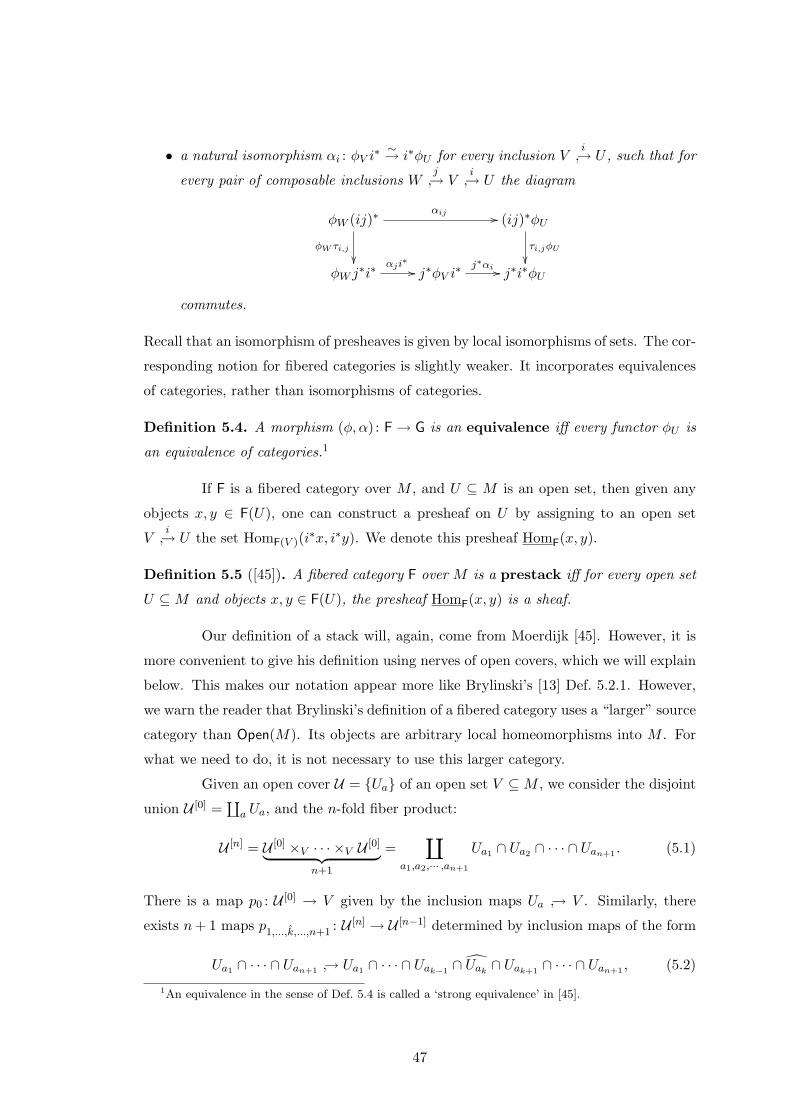
• a natural isomorphism αi : φV i∗∼→ i∗φU for every inclusion V

i→ U , such that for

every pair of composable inclusions Wj→ V

i→ U the diagram

φW (ij)∗

φW τi,j

αij // (ij)∗φU

τi,jφU

φW j∗i∗

αji∗

// j∗φV i∗ j∗αi // j∗i∗φU

commutes.

Recall that an isomorphism of presheaves is given by local isomorphisms of sets. The cor-

responding notion for fibered categories is slightly weaker. It incorporates equivalences

of categories, rather than isomorphisms of categories.

Definition 5.4. A morphism (φ, α) : F→ G is an equivalence iff every functor φU is

an equivalence of categories.1

If F is a fibered category over M , and U ⊆ M is an open set, then given any

objects x, y ∈ F(U), one can construct a presheaf on U by assigning to an open set

Vi→ U the set HomF(V )(i∗x, i∗y). We denote this presheaf HomF(x, y).

Definition 5.5 ([45]). A fibered category F over M is a prestack iff for every open set

U ⊆M and objects x, y ∈ F(U), the presheaf HomF(x, y) is a sheaf.

Our definition of a stack will, again, come from Moerdijk [45]. However, it is

more convenient to give his definition using nerves of open covers, which we will explain

below. This makes our notation appear more like Brylinski’s [13] Def. 5.2.1. However,

we warn the reader that Brylinski’s definition of a fibered category uses a “larger” source

category than Open(M). Its objects are arbitrary local homeomorphisms into M . For

what we need to do, it is not necessary to use this larger category.

Given an open cover U = Ua of an open set V ⊆M , we consider the disjoint

union U [0] =∐a Ua, and the n-fold fiber product:

U [n] = U [0] ×V · · · ×V U [0]︸ ︷︷ ︸n+1

=∐

a1,a2,··· ,an+1

Ua1 ∩ Ua2 ∩ · · · ∩ Uan+1 . (5.1)

There is a map p0 : U [0] → V given by the inclusion maps Ua → V . Similarly, there

exists n+ 1 maps p1,...,k,...,n+1 : U [n] → U [n−1] determined by inclusion maps of the form

Ua1 ∩ · · · ∩ Uan+1 → Ua1 ∩ · · · ∩ Uak−1∩ Uak ∩ Uak+1

∩ · · · ∩ Uan+1 , (5.2)

1An equivalence in the sense of Def. 5.4 is called a ‘strong equivalence’ in [45].

47

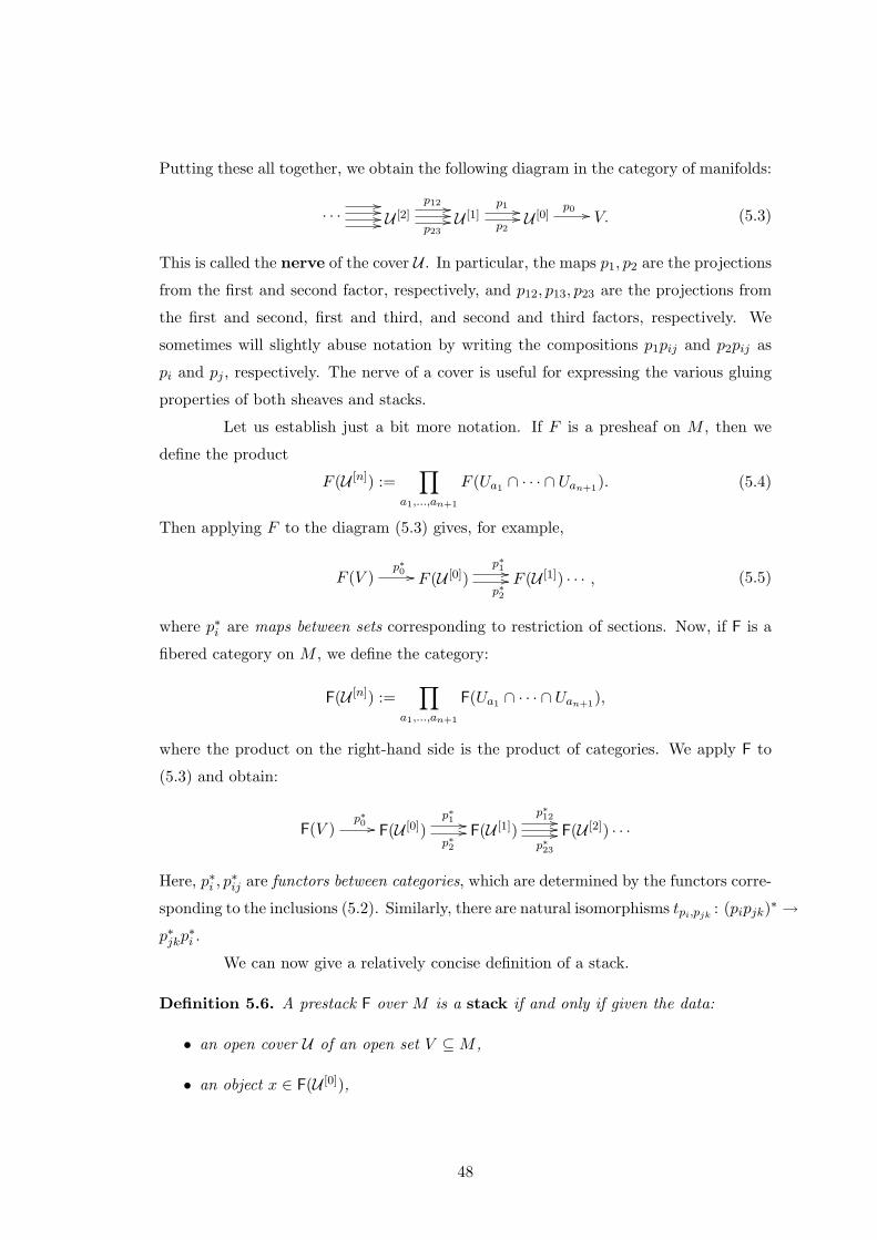
Putting these all together, we obtain the following diagram in the category of manifolds:

· · ·//////// U [2]

p12 ////p23

// U [1]p1 //p2

// U [0]p0 // V. (5.3)

This is called the nerve of the cover U . In particular, the maps p1, p2 are the projections

from the first and second factor, respectively, and p12, p13, p23 are the projections from

the first and second, first and third, and second and third factors, respectively. We

sometimes will slightly abuse notation by writing the compositions p1pij and p2pij as

pi and pj , respectively. The nerve of a cover is useful for expressing the various gluing

properties of both sheaves and stacks.

Let us establish just a bit more notation. If F is a presheaf on M , then we

define the product

F (U [n]) :=∏

a1,...,an+1

F (Ua1 ∩ · · · ∩ Uan+1). (5.4)

Then applying F to the diagram (5.3) gives, for example,

F (V )p∗0 // F (U [0])

p∗1 //p∗2

// F (U [1]) · · · , (5.5)

where p∗i are maps between sets corresponding to restriction of sections. Now, if F is a

fibered category on M , we define the category:

F(U [n]) :=∏

a1,...,an+1

F(Ua1 ∩ · · · ∩ Uan+1),

where the product on the right-hand side is the product of categories. We apply F to

(5.3) and obtain:

F(V )p∗0 // F(U [0])

p∗1 //p∗2

// F(U [1])p∗12 ////p∗23

// F(U [2]) · · ·

Here, p∗i , p∗ij are functors between categories, which are determined by the functors corre-

sponding to the inclusions (5.2). Similarly, there are natural isomorphisms tpi,pjk : (pipjk)∗ →p∗jkp

∗i .

We can now give a relatively concise definition of a stack.

Definition 5.6. A prestack F over M is a stack if and only if given the data:

• an open cover U of an open set V ⊆M ,

• an object x ∈ F(U [0]),

48

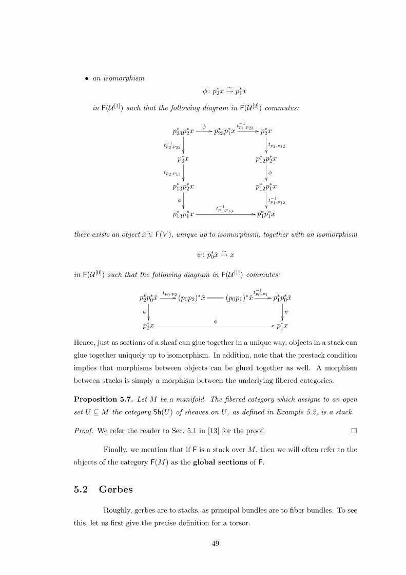
• an isomorphism

φ : p∗2x∼→ p∗1x

in F(U [1]) such that the following diagram in F(U [2]) commutes:

p∗23p∗2x

t−1p2,p23

φ // p∗23p∗1x

t−1p1,p23 // p∗2x

tp2,p12

p∗3x

tp2,p13

p∗12p∗2x

φ

p∗13p

∗2x

φ

p∗12p∗1x

t−1p1,p12

p∗13p

∗1x

t−1p1,p13 // p∗1p

∗1x

there exists an object x ∈ F(V ), unique up to isomorphism, together with an isomorphism

ψ : p∗0x∼→ x

in F(U [0]) such that the following diagram in F(U [1]) commutes:

p∗2p∗0x

ψ

tp0,p2// (p0p2)∗x (p0p1)∗xt−1p0,p1 // p∗1p

∗0x

ψ

p∗2x

φ // p∗1x

Hence, just as sections of a sheaf can glue together in a unique way, objects in a stack can

glue together uniquely up to isomorphism. In addition, note that the prestack condition

implies that morphisms between objects can be glued together as well. A morphism

between stacks is simply a morphism between the underlying fibered categories.

Proposition 5.7. Let M be a manifold. The fibered category which assigns to an open

set U ⊆M the category Sh(U) of sheaves on U , as defined in Example 5.2, is a stack.

Proof. We refer the reader to Sec. 5.1 in [13] for the proof.

Finally, we mention that if F is a stack over M , then we will often refer to the

objects of the category F(M) as the global sections of F.

5.2 Gerbes

Roughly, gerbes are to stacks, as principal bundles are to fiber bundles. To see

this, let us first give the precise definition for a torsor.

49

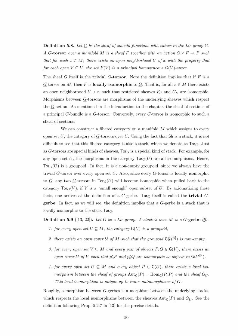
Definition 5.8. Let G be the sheaf of smooth functions with values in the Lie group G.

A G-torsor over a manifold M is a sheaf F together with an action G × F → F such

that for each x ∈ M , there exists an open neighborhood U of x with the property that

for each open V ⊆ U , the set F (V ) is a principal homogeneous G(V )-space.

The sheaf G itself is the trivial G-torsor. Note the definition implies that if F is a

G-torsor on M , then F is locally isomorphic to G. That is, for all x ∈M there exists

an open neighborhood U 3 x, such that restricted sheaves FU and GU are isomorphic.

Morphisms between G-torsors are morphisms of the underlying sheaves which respect

the G-action. As mentioned in the introduction to the chapter, the sheaf of sections of

a principal G-bundle is a G-torsor. Conversely, every G-torsor is isomorphic to such a

sheaf of sections.

We can construct a fibered category on a manifold M which assigns to every

open set U , the category of G-torsors over U . Using the fact that Sh is a stack, it is not

difficult to see that this fibered category is also a stack, which we denote as TorG. Just

as G-torsors are special kinds of sheaves, TorG is a special kind of stack. For example, for

any open set U , the morphisms in the category TorG(U) are all isomorphisms. Hence,

TorG(U) is a groupoid. In fact, it is a non-empty groupoid, since we always have the

trivial G-torsor over every open set U . Also, since every G-torsor is locally isomorphic

to G, any two G-torsors in TorG(U) will become isomorphic when pulled back to the

category TorG(V ), if V is a “small enough” open subset of U . By axiomatizing these

facts, one arrives at the definition of a G-gerbe. TorG itself is called the trivial G-

gerbe. In fact, as we will see, the definition implies that a G-gerbe is a stack that is

locally isomorphic to the stack TorG.

Definition 5.9 ([13, 22]). Let G be a Lie group. A stack G over M is a G-gerbe iff:

1. for every open set U ⊆M , the category G(U) is a groupoid,

2. there exists an open cover U of M such that the groupoid G(U [0]) is non-empty,

3. for every open set V ⊆ M and every pair of objects P,Q ∈ G(V ), there exists an

open cover U of V such that p∗0P and p∗0Q are isomorphic as objects in G(U [0]),

4. for every open set U ⊆ M and every object P ∈ G(U), there exists a local iso-

morphism between the sheaf of groups AutG(P ) = HomG(P, P ) and the sheaf GU .

This local isomorphism is unique up to inner automorphisms of G.

Roughly, a morphism between G-gerbes is a morphism between the underlying stacks,

which respects the local isomorphisms between the sheaves AutG(P ) and GU . See the

definition following Prop. 5.2.7 in [13] for the precise details.

50

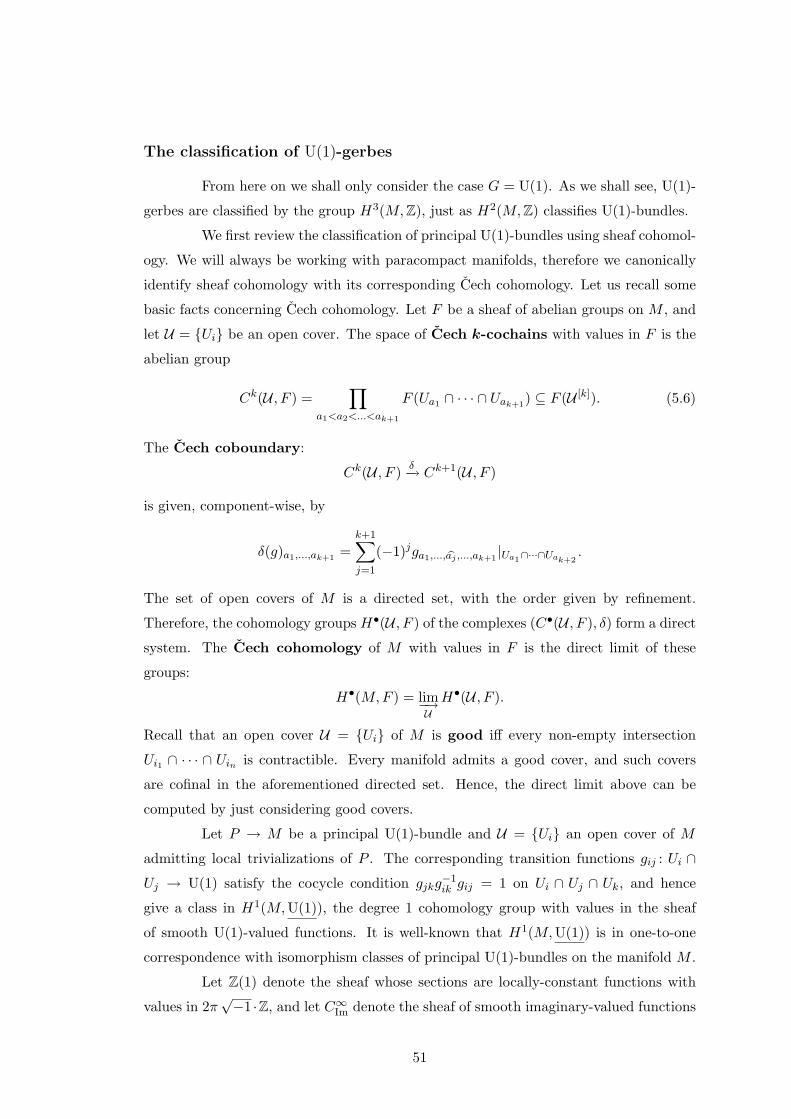
The classification of U(1)-gerbes

From here on we shall only consider the case G = U(1). As we shall see, U(1)-

gerbes are classified by the group H3(M,Z), just as H2(M,Z) classifies U(1)-bundles.

We first review the classification of principal U(1)-bundles using sheaf cohomol-

ogy. We will always be working with paracompact manifolds, therefore we canonically

identify sheaf cohomology with its corresponding Cech cohomology. Let us recall some

basic facts concerning Cech cohomology. Let F be a sheaf of abelian groups on M , and

let U = Ui be an open cover. The space of Cech k-cochains with values in F is the

abelian group

Ck(U , F ) =∏

a1<a2<...<ak+1

F (Ua1 ∩ · · · ∩ Uak+1) ⊆ F (U [k]). (5.6)

The Cech coboundary:

Ck(U , F ) δ−→ Ck+1(U , F )

is given, component-wise, by

δ(g)a1,...,ak+1=

k+1∑j=1

(−1)jga1,..., baj ,...,ak+1|Ua1∩···∩Uak+2

.

The set of open covers of M is a directed set, with the order given by refinement.

Therefore, the cohomology groups H•(U , F ) of the complexes (C•(U , F ), δ) form a direct

system. The Cech cohomology of M with values in F is the direct limit of these

groups:

H•(M,F ) = lim−→UH•(U , F ).

Recall that an open cover U = Ui of M is good iff every non-empty intersection

Ui1 ∩ · · · ∩ Uin is contractible. Every manifold admits a good cover, and such covers

are cofinal in the aforementioned directed set. Hence, the direct limit above can be

computed by just considering good covers.

Let P → M be a principal U(1)-bundle and U = Ui an open cover of M

admitting local trivializations of P . The corresponding transition functions gij : Ui ∩Uj → U(1) satisfy the cocycle condition gjkg

−1ik gij = 1 on Ui ∩ Uj ∩ Uk, and hence

give a class in H1(M,U(1)), the degree 1 cohomology group with values in the sheaf

of smooth U(1)-valued functions. It is well-known that H1(M,U(1)) is in one-to-one

correspondence with isomorphism classes of principal U(1)-bundles on the manifold M .

Let Z(1) denote the sheaf whose sections are locally-constant functions with

values in 2π√−1 ·Z, and let C∞Im denote the sheaf of smooth imaginary-valued functions

51

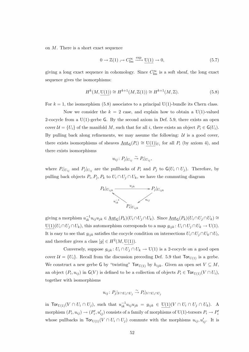
on M . There is a short exact sequence

0→ Z(1) → C∞Imexp−−→ U(1)→ 0, (5.7)

giving a long exact sequence in cohomology. Since C∞Im is a soft sheaf, the long exact

sequence gives the isomorphisms:

Hk(M,U(1)) ∼= Hk+1(M,Z(1)) ∼= Hk+1(M,Z). (5.8)

For k = 1, the isomorphism (5.8) associates to a principal U(1)-bundle its Chern class.

Now we consider the k = 2 case, and explain how to obtain a U(1)-valued

2-cocycle from a U(1)-gerbe G. By the second axiom in Def. 5.9, there exists an open

cover U = Ui of the manifold M , such that for all i, there exists an object Pi ∈ G(Ui).

By pulling back along refinements, we may assume the following: U is a good cover,

there exists isomorphisms of sheaves AutG(Pi) ∼= U(1)|Ui for all Pi (by axiom 4), and

there exists isomorphisms

uij : Pj |Uij∼→ Pi|Uij ,

where Pi|Uij and Pj |Uij are the pullbacks of Pi and Pj to G(Ui ∩ Uj). Therefore, by

pulling back objects Pi, Pj , Pk to Ui ∩ Uj ∩ Uk, we have the commuting diagram

Pk|Uijkujk // Pj |Uijk

uijzzuuuuuuuuu

Pi|Uijku−1ik

ddIIIIIIIII

giving a morphism u−1ik uijujk ∈ AutG(Pk)(Ui∩Uj ∩Uk). Since AutG(Pk)(Ui∩Uj ∩Uk) ∼=

U(1)(Ui ∩Uj ∩Uk), this automorphism corresponds to a map gijk : Ui ∩Uj ∩Uk → U(1).

It is easy to see that gijk satisfies the cocycle condition on intersections Ui∩Uj ∩Uk∩Ul,and therefore gives a class [g] ∈ H2(M,U(1)).

Conversely, suppose gijk : Ui ∩ Uj ∩ Uk → U(1) is a 2-cocycle on a good open

cover U = Ui. Recall from the discussion preceding Def. 5.9 that TorU(1) is a gerbe.

We construct a new gerbe G by “twisting” TorU(1) by hijk. Given an open set V ⊆ M ,

an object (Pi, uij) in G(V ) is defined to be a collection of objects Pi ∈ TorU(1)(V ∩ Ui),together with isomorphisms

uij : Pj |V ∩Ui∩Uj∼→ Pi|V ∩Ui∩Uj

in TorU(1)(V ∩ Ui ∩ Uj), such that u−1ik uijujk = gijk ∈ U(1)(V ∩ Ui ∩ Uj ∩ Uk). A

morphism (Pi, uij)→ (P ′i , u′ij) consists of a family of morphisms of U(1)-torsors Pi → P ′i

whose pullbacks in TorU(1)(V ∩ Ui ∩ Uj) commute with the morphisms uij , u′ij . It is

52

straightforward to show that by using the pullback functors defined for TorU(1), we

obtain a stack G in this way. To see that AutG(Pi, uij) is locally isomorphic to U(1),

note that such an automorphism must be given by a collection of morphisms Pi∼→

Pi corresponding to sections in U(1)(V ∩ Ui), which must agree when pulled back to

V ∩Ui∩Uj . These glue to give a section in U(1)(V ), thereby establishing an isomorphism

AutG(Pi, uij)(V ) ∼= U(1)(V ). To show that the other axioms in Def. 5.9 hold, one may

show that the categories G(Ui) and TorU(1)(Ui) are equivalent for all Ui. (This follows

from the fact that gijk restricted to Ui is a 2-coboundary since H2(Ui,U(1)) = 0. See

Sec. 5.2 in [13].) This construction, combined with the isomorphism (5.8) leads to the

following theorem:

Theorem 5.10 ([13, 22]). There is a one-to-one correspondence between equivalence

classes of U(1)-gerbes on a manifold M and classes in H3(M,Z).

In fact, one can go further and define the product of two U(1)-gerbes, which is similar

to the contracted product of principal U(1)-bundles. The set of equivalence classes of

U(1)-gerbes therefore form an abelian group, and the bijection in the above theorem

lifts to an isomorphism of groups.

U(1)-gerbes can be equipped with structures that are the higher analogs of

connections and curvature. To classify these, we need to introduce a more sophisticated

cohomology theory.

5.3 Deligne cohomology

To motivate this section, let us return to the familiar case of principal bundles.

If P → M is a principal U(1)-bundle equipped with a connection, then, in addition to

the transition functions gij , we have local 1-forms θi ∈ Ω1(Ui) satisfying a cocycle-like

condition√−1 · (θi − θj) = g−1

ij dgij on Ui ∩ Uj . The curvature of the connection is the

global 2-form ω on M satisfying ω|Ui = dθi.

The classification of principal U(1)-bundles equipped with connection requires

a refinement of the Cech cohomology group H1(M,U(1)). The purpose of real Deligne

cohomology is to make this notion precise. In fact, as we will see, Deligne cohomology

provides such a refinement for any geometric objects classified by Hk(M,Z) for arbitrary

k.

The primary reference for what follows is Sec. 1.5 of Brylinski [13]. However,

Brylinski works with the group C× instead of U(1). What we call real Deligne cohomol-

ogy is presented, without proofs, in Sec. 3 of Carey, Johnson, and Murray [17].

53

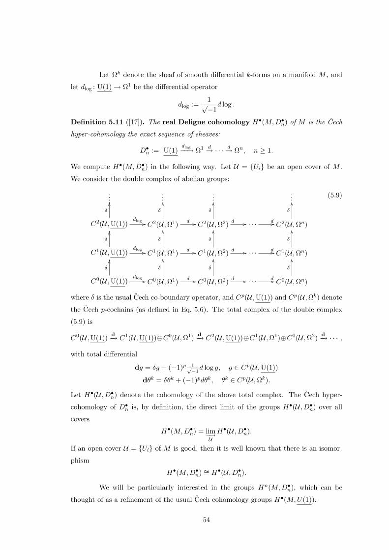
Let Ωk denote the sheaf of smooth differential k-forms on a manifold M , and

let dlog : U(1)→ Ω1 be the differential operator

dlog :=1√−1

d log .

Definition 5.11 ([17]). The real Deligne cohomology H•(M,D•n) of M is the Cech

hyper-cohomology the exact sequence of sheaves:

D•n := U(1)dlog−−→ Ω1 d→ · · · d→ Ωn, n ≥ 1.

We compute H•(M,D•n) in the following way. Let U = Ui be an open cover of M .

We consider the double complex of abelian groups:

......

......

C2(U ,U(1))

δ

OO

dlog // C2(U ,Ω1)

δ

OO

d // C2(U ,Ω2)

δ

OO

d // · · · d // C2(U ,Ωn)

δ

OO

C1(U ,U(1))

δ

OO

dlog // C1(U ,Ω1)

δ

OO

d // C1(U ,Ω2)

δ

OO

d // · · · d // C1(U ,Ωn)

δ

OO

C0(U ,U(1))

δ

OO

dlog // C0(U ,Ω1)

δ

OO

d // C0(U ,Ω2)

δ

OO

d // · · · d // C0(U ,Ωn)

δ

OO

(5.9)

where δ is the usual Cech co-boundary operator, and Cp(U ,U(1)) and Cp(U ,Ωk) denote

the Cech p-cochains (as defined in Eq. 5.6). The total complex of the double complex

(5.9) is

C0(U ,U(1)) d−→ C1(U ,U(1))⊕C0(U ,Ω1) d−→ C2(U ,U(1))⊕C1(U ,Ω1)⊕C0(U ,Ω2) d−→ · · · ,

with total differential

dg = δg + (−1)p 1√−1d log g, g ∈ Cp(U ,U(1))

dθk = δθk + (−1)pdθk, θk ∈ Cp(U ,Ωk).

Let H•(U , D•n) denote the cohomology of the above total complex. The Cech hyper-

cohomology of D•n is, by definition, the direct limit of the groups H•(U , D•n) over all

covers

H•(M,D•n) = lim−→UH•(U , D•n).

If an open cover U = Ui of M is good, then it is well known that there is an isomor-

phism

H•(M,D•n) ∼= H•(U , D•n).

We will be particularly interested in the groups Hn(M,D•n), which can be

thought of as a refinement of the usual Cech cohomology groups H•(M,U(1)).

54

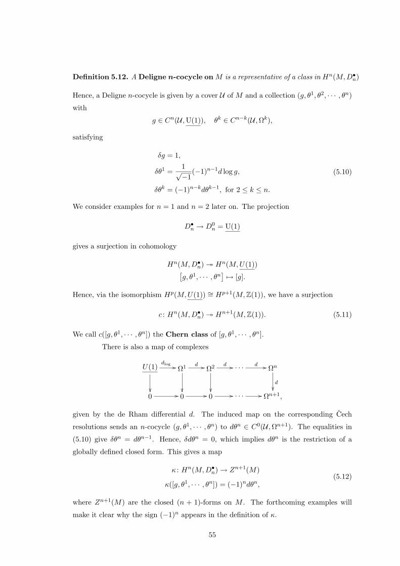
Definition 5.12. A Deligne n-cocycle on M is a representative of a class in Hn(M,D•n)

Hence, a Deligne n-cocycle is given by a cover U of M and a collection (g, θ1, θ2, · · · , θn)

with

g ∈ Cn(U ,U(1)), θk ∈ Cn−k(U ,Ωk),

satisfying

δg = 1,

δθ1 =1√−1

(−1)n−1d log g,

δθk = (−1)n−kdθk−1, for 2 ≤ k ≤ n.

(5.10)

We consider examples for n = 1 and n = 2 later on. The projection

D•n → D0n = U(1)

gives a surjection in cohomology

Hn(M,D•n) Hn(M,U(1))[g, θ1, · · · , θn

]7→ [g].

Hence, via the isomorphism Hp(M,U(1)) ∼= Hp+1(M,Z(1)), we have a surjection

c : Hn(M,D•n) Hn+1(M,Z(1)). (5.11)

We call c([g, θ1, · · · , θn]) the Chern class of [g, θ1, · · · , θn].

There is also a map of complexes

U(1)

dlog // Ω1

d // Ω2

d // · · · d // Ωn

d

0 // 0 // 0 // · · · // Ωn+1,

given by the de Rham differential d. The induced map on the corresponding Cech

resolutions sends an n-cocycle (g, θ1, · · · , θn) to dθn ∈ C0(U ,Ωn+1). The equalities in

(5.10) give δθn = dθn−1. Hence, δdθn = 0, which implies dθn is the restriction of a

globally defined closed form. This gives a map

κ : Hn(M,D•n)→ Zn+1(M)

κ([g, θ1, · · · , θn]) = (−1)ndθn,(5.12)

where Zn+1(M) are the closed (n + 1)-forms on M . The forthcoming examples will

make it clear why the sign (−1)n appears in the definition of κ.

55

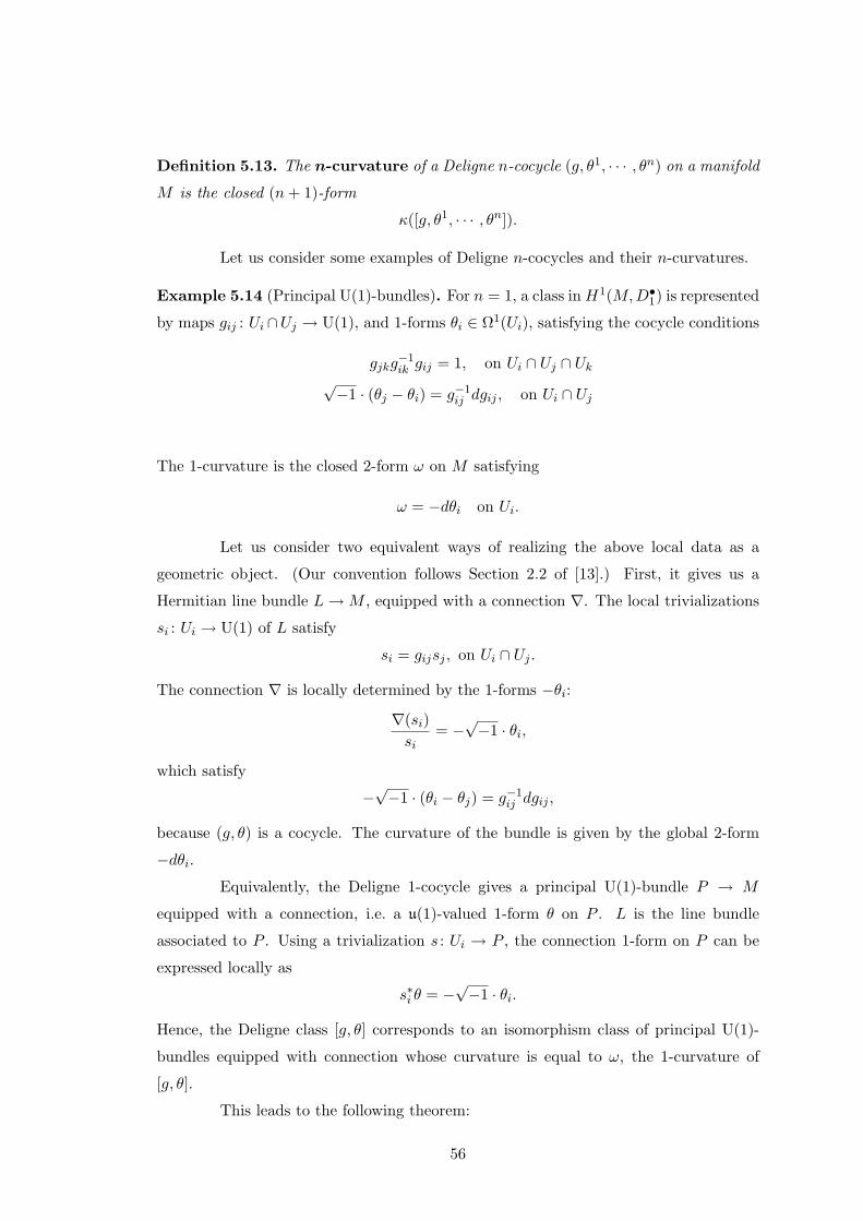
Definition 5.13. The n-curvature of a Deligne n-cocycle (g, θ1, · · · , θn) on a manifold

M is the closed (n+ 1)-form

κ([g, θ1, · · · , θn]).

Let us consider some examples of Deligne n-cocycles and their n-curvatures.

Example 5.14 (Principal U(1)-bundles). For n = 1, a class in H1(M,D•1) is represented

by maps gij : Ui ∩Uj → U(1), and 1-forms θi ∈ Ω1(Ui), satisfying the cocycle conditions

gjkg−1ik gij = 1, on Ui ∩ Uj ∩ Uk

√−1 · (θj − θi) = g−1

ij dgij , on Ui ∩ Uj

The 1-curvature is the closed 2-form ω on M satisfying

ω = −dθi on Ui.

Let us consider two equivalent ways of realizing the above local data as a

geometric object. (Our convention follows Section 2.2 of [13].) First, it gives us a

Hermitian line bundle L→M , equipped with a connection ∇. The local trivializations

si : Ui → U(1) of L satisfy

si = gijsj , on Ui ∩ Uj .

The connection ∇ is locally determined by the 1-forms −θi:

∇(si)si

= −√−1 · θi,

which satisfy

−√−1 · (θi − θj) = g−1

ij dgij ,

because (g, θ) is a cocycle. The curvature of the bundle is given by the global 2-form

−dθi.Equivalently, the Deligne 1-cocycle gives a principal U(1)-bundle P → M

equipped with a connection, i.e. a u(1)-valued 1-form θ on P . L is the line bundle

associated to P . Using a trivialization s : Ui → P , the connection 1-form on P can be

expressed locally as

s∗i θ = −√−1 · θi.

Hence, the Deligne class [g, θ] corresponds to an isomorphism class of principal U(1)-

bundles equipped with connection whose curvature is equal to ω, the 1-curvature of

[g, θ].

This leads to the following theorem:

56

Theorem 5.15 ([13]). The group of isomorphism classes of principal U(1)-bundles with

connection, on a manifold M , and the degree one Deligne cohomology group H1(M,D•1)

are isomorphic.

Example 5.16 (U(1)-gerbes). The n = 2 case will be particularly relevant for our

work in the subsequent chapters. A class [g,A,B] ∈ H2(M,D•2) is represented by maps

gijk : Ui∩Uj∩Uk → U(1), 1-forms Aij ∈ Ω1(Ui∩Uj), and 2-forms Bi ∈ Ω2(Ui) satisfying

the cocycle conditions:

gjklg−1ikl gijlg

−1ijk = 1 on Ui ∩ Uj ∩ Uk ∩ Ul,

√−1 · (Ajk −Aik +Aij) = −g−1

ijkdgijk on Ui ∩ Uj ∩ Uk,

Bj −Bi = dAij on Ui ∩ Uj .

(5.13)

The 2-curvature is the closed 3-form ω on M satisfying

ω = dBi on Ui.

We will see in Section 5.4 that[g,A,B

]corresponds to an isomorphism class of a U(1)-

gerbe equipped with a 2-connection whose 2-curvature is ω.

Integral differential forms

In the remainder of this section, we determine which closed differential forms

can be realized as the n-curvature of a Deligne cocycle. Let R(1) denote the sheaf whose

sections are locally-constant functions with values in√−1 · R.

Definition 5.17. A closed differential form ω ∈ Ωk(M) is integral iff the class√−1·[ω]

lies in the image of the composition

Hk(M,Z(1))→ Hk(M,R(1)) ∼→√−1 ·Hk

dR(M). (5.14)

We denote by Zk(M)int the subspace of all closed integral k-forms on M .

Our goal is to show that the n-curvature of a Deligne n-cocycle is an integral (n+1)-form,

and conversely, every integral (n+ 1)-form is the curvature of some Deligne n-cocycle.

We begin by introducing some necessary technical machinery. Let Ω1≤•≤k de-

note the complex of sheaves Ω1 d→ · · · d→ Ωk on a manifold M . Let R be the sheaf of lo-

cally constant R-valued functions. Let dimM = m. We consider the hyper-cohomology

57

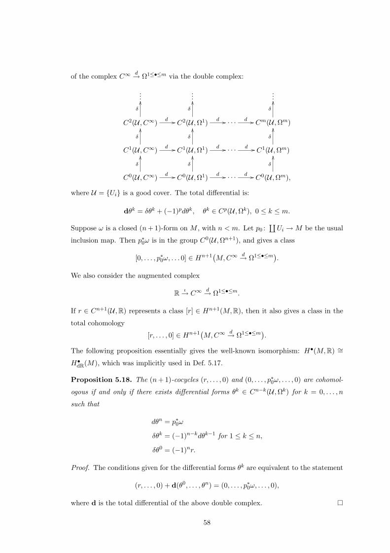
of the complex C∞ d→ Ω1≤•≤m via the double complex:

......

...

C2(U , C∞)

δ

OO

d // C2(U ,Ω1)

δ

OO

d // · · · d // Cm(U ,Ωm)

δ

OO

C1(U , C∞)

δ

OO

d // C1(U ,Ω1)

δ

OO

d // · · · d // C1(U ,Ωm)

δ

OO

C0(U , C∞)

δ

OO

d // C0(U ,Ω1)

δ

OO

d // · · · d // C0(U ,Ωm),

δ

OO

where U = Ui is a good cover. The total differential is:

dθk = δθk + (−1)pdθk, θk ∈ Cp(U ,Ωk), 0 ≤ k ≤ m.

Suppose ω is a closed (n+ 1)-form on M , with n < m. Let p0 :∐Ui →M be the usual

inclusion map. Then p∗0ω is in the group C0(U ,Ωn+1), and gives a class

[0, . . . , p∗0ω, . . . 0] ∈ Hn+1(M,C∞

d→ Ω1≤•≤m).We also consider the augmented complex

R ι→ C∞d→ Ω1≤•≤m.

If r ∈ Cn+1(U ,R) represents a class [r] ∈ Hn+1(M,R), then it also gives a class in the

total cohomology

[r, . . . , 0] ∈ Hn+1(M,C∞

d→ Ω1≤•≤m).The following proposition essentially gives the well-known isomorphism: H•(M,R) ∼=H•dR(M), which was implicitly used in Def. 5.17.

Proposition 5.18. The (n+ 1)-cocycles (r, . . . , 0) and (0, . . . , p∗0ω, . . . , 0) are cohomol-

ogous if and only if there exists differential forms θk ∈ Cn−k(U ,Ωk) for k = 0, . . . , n

such that

dθn = p∗0ω

δθk = (−1)n−kdθk−1 for 1 ≤ k ≤ n,

δθ0 = (−1)nr.

Proof. The conditions given for the differential forms θk are equivalent to the statement

(r, . . . , 0) + d(θ0, . . . , θn) = (0, . . . , p∗0ω, . . . , 0),

where d is the total differential of the above double complex.

58

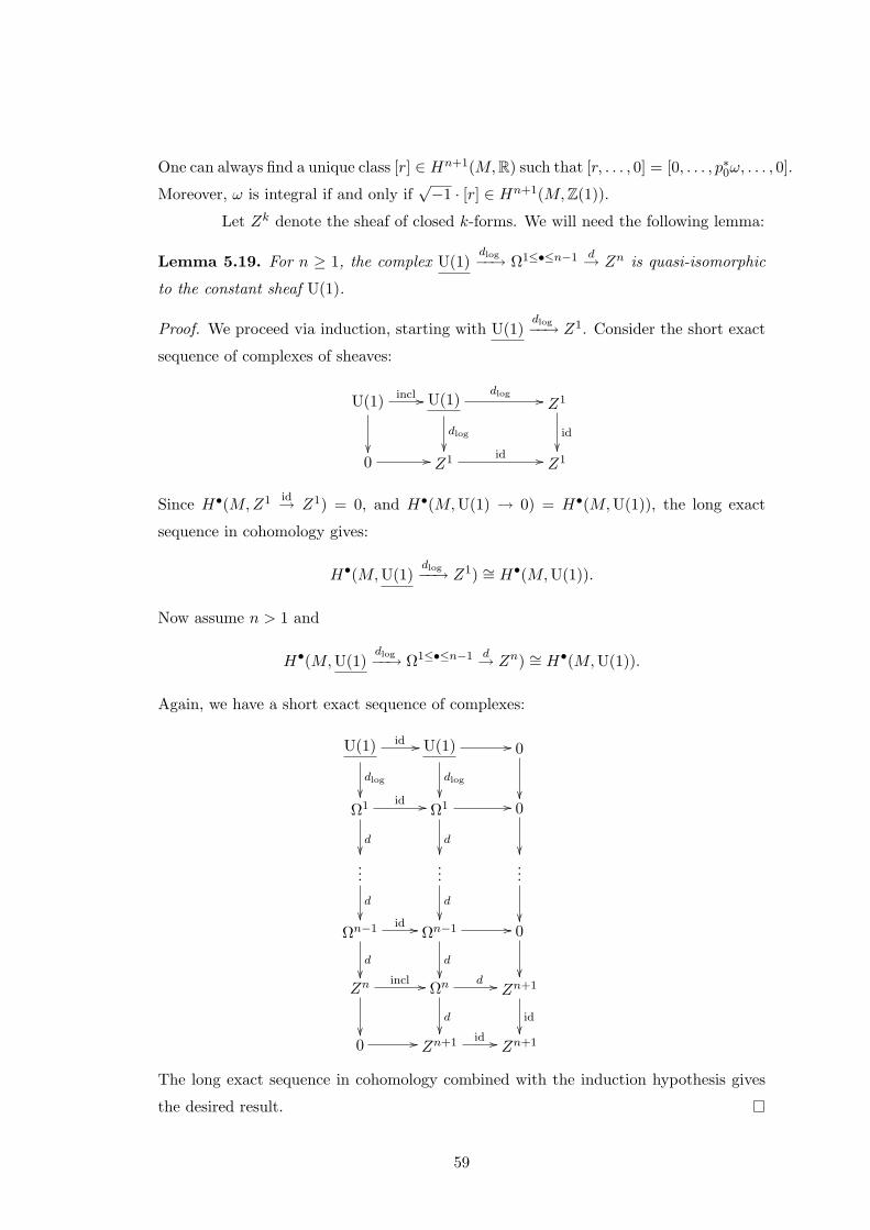
One can always find a unique class [r] ∈ Hn+1(M,R) such that [r, . . . , 0] = [0, . . . , p∗0ω, . . . , 0].

Moreover, ω is integral if and only if√−1 · [r] ∈ Hn+1(M,Z(1)).

Let Zk denote the sheaf of closed k-forms. We will need the following lemma:

Lemma 5.19. For n ≥ 1, the complex U(1)dlog−−→ Ω1≤•≤n−1 d→ Zn is quasi-isomorphic

to the constant sheaf U(1).

Proof. We proceed via induction, starting with U(1)dlog−−→ Z1. Consider the short exact

sequence of complexes of sheaves:

U(1)

incl // U(1)

dlog

dlog // Z1

id

0 // Z1 id // Z1

Since H•(M,Z1 id→ Z1) = 0, and H•(M,U(1) → 0) = H•(M,U(1)), the long exact

sequence in cohomology gives:

H•(M,U(1)dlog−−→ Z1) ∼= H•(M,U(1)).

Now assume n > 1 and

H•(M,U(1)dlog−−→ Ω1≤•≤n−1 d→ Zn) ∼= H•(M,U(1)).

Again, we have a short exact sequence of complexes:

U(1)

dlog

id // U(1)

dlog

// 0

Ω1

d

id // Ω1

d

// 0

...d

...d

...

Ωn−1

d

id // Ωn−1

d

// 0

Zn

incl // Ωn

d

d // Zn+1

id

0 // Zn+1 id // Zn+1

The long exact sequence in cohomology combined with the induction hypothesis gives

the desired result.

59

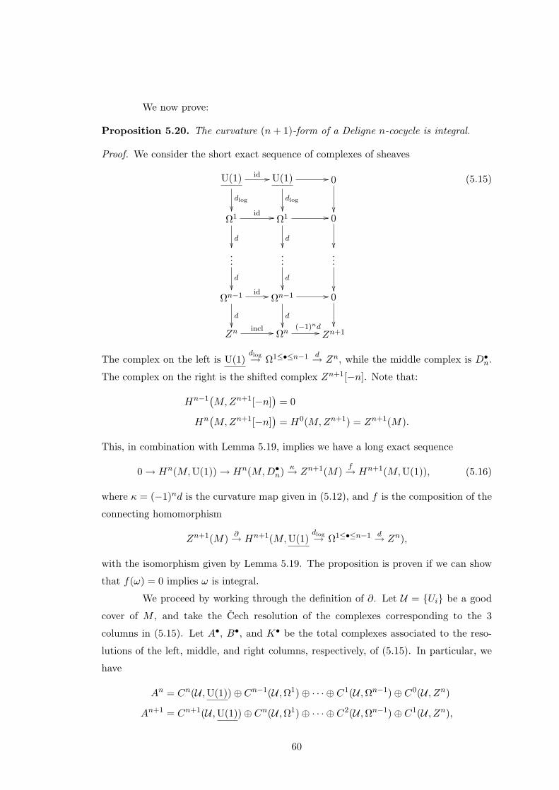
We now prove:

Proposition 5.20. The curvature (n+ 1)-form of a Deligne n-cocycle is integral.

Proof. We consider the short exact sequence of complexes of sheaves

U(1)

dlog

id // U(1)

dlog

// 0

Ω1

d

id // Ω1

d

// 0

...d

...d

...

Ωn−1

d

id // Ωn−1

d

// 0

Zn

incl // Ωn(−1)nd// Zn+1

(5.15)

The complex on the left is U(1)dlog→ Ω1≤•≤n−1 d→ Zn, while the middle complex is D•n.

The complex on the right is the shifted complex Zn+1[−n]. Note that:

Hn−1(M,Zn+1[−n]

)= 0

Hn(M,Zn+1[−n]

)= H0(M,Zn+1) = Zn+1(M).

This, in combination with Lemma 5.19, implies we have a long exact sequence

0→ Hn(M,U(1))→ Hn(M,D•n) κ→ Zn+1(M)f→ Hn+1(M,U(1)), (5.16)

where κ = (−1)nd is the curvature map given in (5.12), and f is the composition of the

connecting homomorphism

Zn+1(M) ∂→ Hn+1(M,U(1)dlog→ Ω1≤•≤n−1 d→ Zn),

with the isomorphism given by Lemma 5.19. The proposition is proven if we can show

that f(ω) = 0 implies ω is integral.

We proceed by working through the definition of ∂. Let U = Ui be a good

cover of M , and take the Cech resolution of the complexes corresponding to the 3

columns in (5.15). Let A•, B•, and K• be the total complexes associated to the reso-

lutions of the left, middle, and right columns, respectively, of (5.15). In particular, we

have

An = Cn(U ,U(1))⊕ Cn−1(U ,Ω1)⊕ · · · ⊕ C1(U ,Ωn−1)⊕ C0(U , Zn)

An+1 = Cn+1(U ,U(1))⊕ Cn(U ,Ω1)⊕ · · · ⊕ C2(U ,Ωn−1)⊕ C1(U , Zn),

60

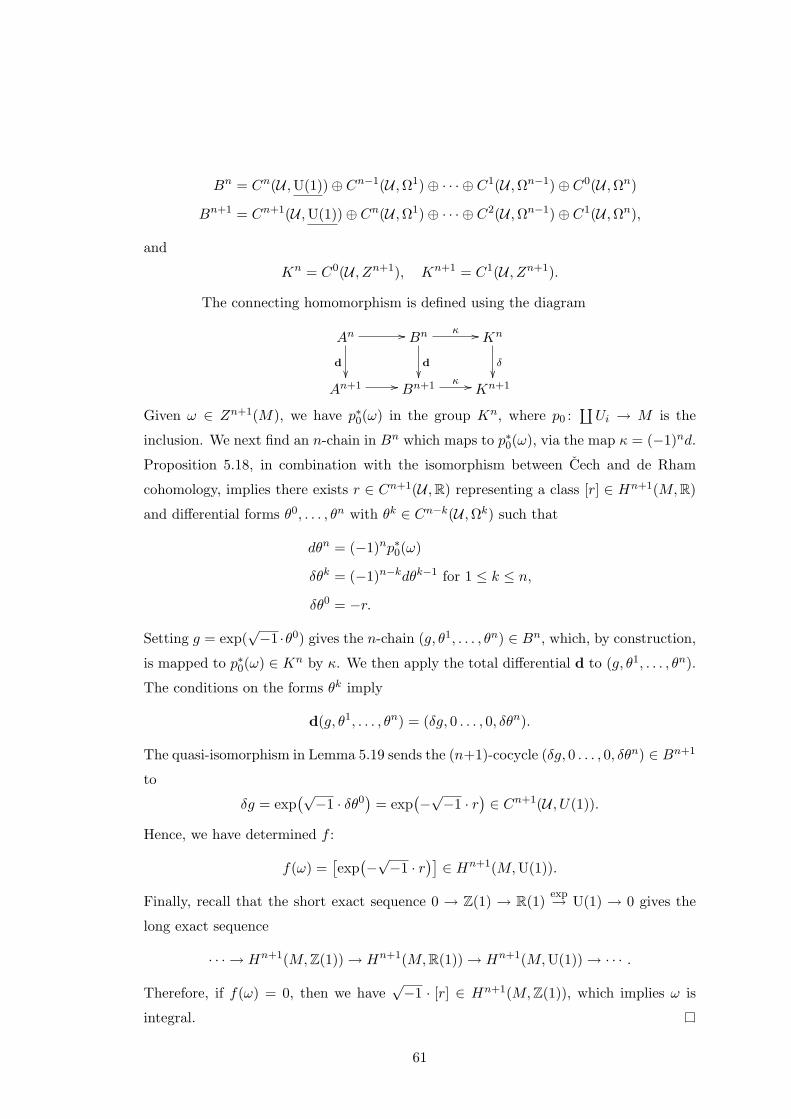
Bn = Cn(U ,U(1))⊕ Cn−1(U ,Ω1)⊕ · · · ⊕ C1(U ,Ωn−1)⊕ C0(U ,Ωn)

Bn+1 = Cn+1(U ,U(1))⊕ Cn(U ,Ω1)⊕ · · · ⊕ C2(U ,Ωn−1)⊕ C1(U ,Ωn),

and

Kn = C0(U , Zn+1), Kn+1 = C1(U , Zn+1).

The connecting homomorphism is defined using the diagram

An

d

// Bn

d

κ // Kn

δ

An+1 // Bn+1 κ // Kn+1

Given ω ∈ Zn+1(M), we have p∗0(ω) in the group Kn, where p0 :∐Ui → M is the

inclusion. We next find an n-chain in Bn which maps to p∗0(ω), via the map κ = (−1)nd.

Proposition 5.18, in combination with the isomorphism between Cech and de Rham

cohomology, implies there exists r ∈ Cn+1(U ,R) representing a class [r] ∈ Hn+1(M,R)

and differential forms θ0, . . . , θn with θk ∈ Cn−k(U ,Ωk) such that

dθn = (−1)np∗0(ω)

δθk = (−1)n−kdθk−1 for 1 ≤ k ≤ n,

δθ0 = −r.

Setting g = exp(√−1 ·θ0) gives the n-chain (g, θ1, . . . , θn) ∈ Bn, which, by construction,

is mapped to p∗0(ω) ∈ Kn by κ. We then apply the total differential d to (g, θ1, . . . , θn).

The conditions on the forms θk imply

d(g, θ1, . . . , θn) = (δg, 0 . . . , 0, δθn).

The quasi-isomorphism in Lemma 5.19 sends the (n+1)-cocycle (δg, 0 . . . , 0, δθn) ∈ Bn+1

to

δg = exp(√−1 · δθ0

)= exp

(−√−1 · r

)∈ Cn+1(U , U(1)).

Hence, we have determined f :

f(ω) =[exp(−√−1 · r

)]∈ Hn+1(M,U(1)).

Finally, recall that the short exact sequence 0 → Z(1) → R(1)exp→ U(1) → 0 gives the

long exact sequence

· · · → Hn+1(M,Z(1))→ Hn+1(M,R(1))→ Hn+1(M,U(1))→ · · · .

Therefore, if f(ω) = 0, then we have√−1 · [r] ∈ Hn+1(M,Z(1)), which implies ω is

integral.

61

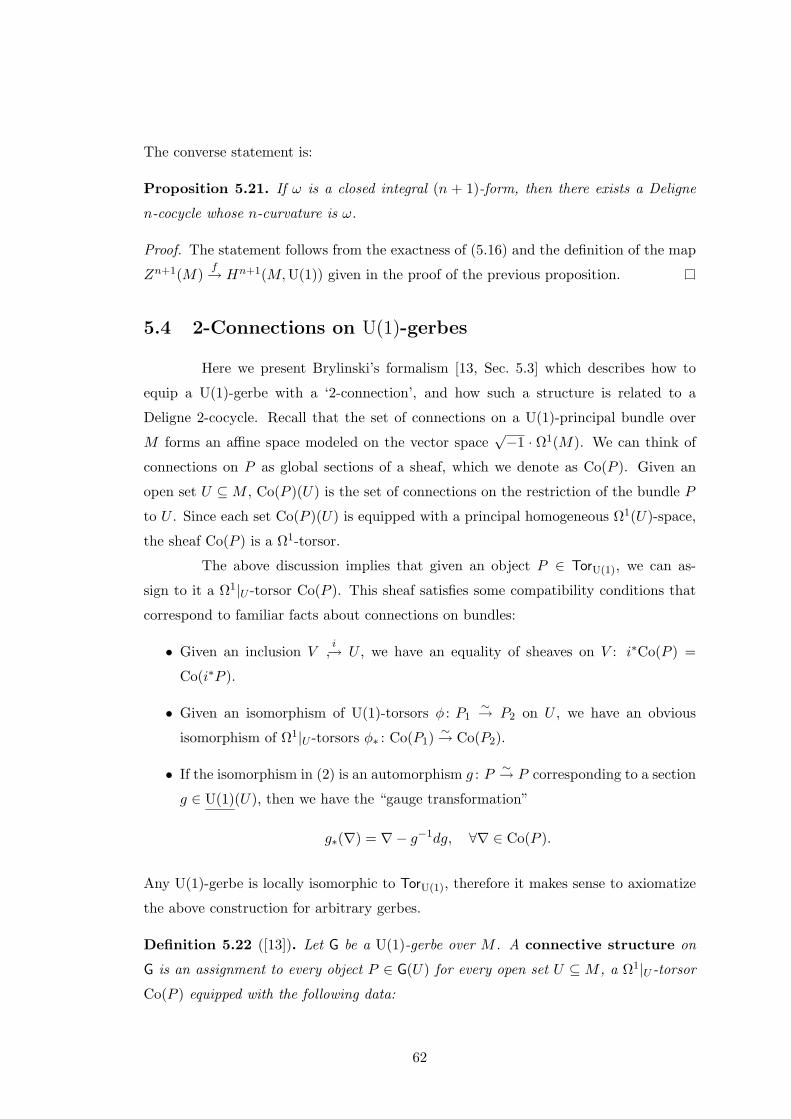
The converse statement is:

Proposition 5.21. If ω is a closed integral (n + 1)-form, then there exists a Deligne

n-cocycle whose n-curvature is ω.

Proof. The statement follows from the exactness of (5.16) and the definition of the map

Zn+1(M)f→ Hn+1(M,U(1)) given in the proof of the previous proposition.

5.4 2-Connections on U(1)-gerbes

Here we present Brylinski’s formalism [13, Sec. 5.3] which describes how to

equip a U(1)-gerbe with a ‘2-connection’, and how such a structure is related to a

Deligne 2-cocycle. Recall that the set of connections on a U(1)-principal bundle over

M forms an affine space modeled on the vector space√−1 · Ω1(M). We can think of

connections on P as global sections of a sheaf, which we denote as Co(P ). Given an

open set U ⊆M , Co(P )(U) is the set of connections on the restriction of the bundle P

to U . Since each set Co(P )(U) is equipped with a principal homogeneous Ω1(U)-space,

the sheaf Co(P ) is a Ω1-torsor.

The above discussion implies that given an object P ∈ TorU(1), we can as-

sign to it a Ω1|U -torsor Co(P ). This sheaf satisfies some compatibility conditions that

correspond to familiar facts about connections on bundles:

• Given an inclusion Vi→ U , we have an equality of sheaves on V : i∗Co(P ) =

Co(i∗P ).

• Given an isomorphism of U(1)-torsors φ : P1∼→ P2 on U , we have an obvious

isomorphism of Ω1|U -torsors φ∗ : Co(P1) ∼→ Co(P2).

• If the isomorphism in (2) is an automorphism g : P ∼→ P corresponding to a section

g ∈ U(1)(U), then we have the “gauge transformation”

g∗(∇) = ∇− g−1dg, ∀∇ ∈ Co(P ).

Any U(1)-gerbe is locally isomorphic to TorU(1), therefore it makes sense to axiomatize

the above construction for arbitrary gerbes.

Definition 5.22 ([13]). Let G be a U(1)-gerbe over M . A connective structure on

G is an assignment to every object P ∈ G(U) for every open set U ⊆M , a Ω1|U -torsor

Co(P ) equipped with the following data:

62

1. For every inclusion Vi→ U , an isomorphism of Ω1|V -torsors

αi : i∗Co(P ) ∼→ Co(i∗P ),

where i∗Co(P ) is the pullback of Co(P ) as an object in Sh(U), such that for any

composable pair Wj→ V

i→ U the diagram

j∗i∗Co(P )j∗αi // j∗Co(i∗P )

αj // Co(j∗i∗P )

ti,j∗

(ij)∗Co(P )αij // Co((ij)∗P )

commutes.

2. For any isomorphisms φ : P1∼→ P2 and ψ : P2

∼→ P3 in G(U), isomorphisms of

Ω1|U -torsors

φ∗ : Co(P1) ∼→ Co(P2), ψ∗ : Co(P2) ∼→ Co(P3),

such that (ψ φ)∗ = ψ∗ φ∗ and the diagram

i∗Co(P1)

α1,i

i∗φ∗ // i∗Co(P2)

α2,i

Co(i∗P1)

(i∗φ)∗ // Co(i∗P2).

commutes. Moreover, if AutG(P )(U) ∼= U(1)(U) and g ∈ U(1)(U), then g∗ : Co(P ) ∼→Co(P ) is the map

∇ 7→ ∇− g−1dg.

If Co(P ) is the sheaf of connections on a principal U(1)-bundle P → M , then

to each section ∇ ∈ Co(P ), we can assign a 2-form K(∇) on M corresponding to its

curvature. This fact motivates the next definition.

Definition 5.23 ([13]). Let G be a U(1)-gerbe over M equipped with a connective struc-

ture P 7→ Co(P ). A curving of the connective structure is an assignment to every

object P ∈ G(U), and every section ∇ ∈ Co(P )(U), for every open set U ⊆M , a 2-form

K(∇) ∈ Ω2(U) with the following properties:

1. Given an inclusion Vi→ U of open sets, and the associated isomorphism αi : i∗Co(P ) ∼→

Co(i∗P ), the equality

K(αi(i∗∇)) = i∗K(∇)

holds, where i∗K(∇) is the usual pullback of differential forms.

63

2. Given an isomorphism φ : P ∼→ P ′ in G(U) and the associated isomorphism φ∗ : Co(P )→Co(P ′), the equality

K(∇) = K(φ∗(∇))

holds.

3. If θ is a 1-form on U , then K(∇+√−1 · θ) = K(∇) + dθ.

We say G is U(1)-gerbe equipped with a 2-connection iff it is equipped with a connective

structure and a curving.

Finally, let us describe how 2-connections are related to Deligne 2-cocycles.

Let G be a U(1)-gerbe on M equipped with a 2-connection. As we described in Section

5.2, we may choose a cover Ui such that there exists objects Pi ∈ G(Ui), isomorphisms

uij : Pj |Uij∼→ Pi|Uij in G(Ui∩Uj), and a 2-cocycle gijk = u−1

ik uijujk ∈ AutG(Pk)(Ui∩Uj∩Uk) ∼= U(1)(Ui∩Uj∩Uk). We choose a section∇i ∈ Co(Pi)(Ui) for each i. The restriction

of ∇i to Ui ∩Uj gives a section of Co(Pi|Uij ) by axiom 1 of Def. 5.22, which we will also

denote as ∇i. The isomorphisms uij induce isomorphisms uij∗ : Co(Pj |Uij )∼→ Co(Pi|Uij )

of Ω1|Uij -torsors. Hence, ∇i and uij∗∇j are both sections of Co(Pi|Uij ). This implies

that there exists 1-forms Aij on Ui ∩ Uj such that

√−1 ·Aij = ∇i − uij∗∇j . (5.17)

Restricting the above equalities to Ui ∩ Uj ∩ Uk gives

√−1 · (Ajk −Aik +Aij) = ∇i − (u−1

ik uijujk)∗∇i.

Axiom 2 of Def. 5.22 implies that the right-hand side of this equation is gijkdgijk. Hence,

√−1 · (Ajk −Aik +Aij) = gijkdgijk.

The curving on G assigns a 2-form Bi = K(∇i) on each Ui. On the intersections

Ui ∩ Uj , axiom 1 of Def. 5.23 implies that K(∇i) is just the restriction of Bi. It follows

from axiom 2 of the same definition that

Bj = K(∇j) = K(uij∗∇j),

and, by applying K to Eq. 5.17, we obtain

Bi −Bj = dAij .

By comparing these calculations with Eqs. 5.13 in Example 5.16, we see that we’ve

obtained from G a Deligne 2-cocycle (g,−A,B) whose 2-curvature is given by the 3-

form ω = dBi. This leads to the following theorem.

64

Theorem 5.24 ([13]). There is a one-to-one correspondence between the set of equiv-

alence classes of U(1)-gerbes with 2-connection on a manifold M and the degree two

Deligne cohomology group H2(M,D•2).

5.5 2-Line stacks

The category of principal U(1)-bundles with connection over a manifold is

equivalent to the category of Hermitian line bundles with connection. This equivalence

sends a principal bundle to its associated line bundle. The goal of this section is to

construct an analogous associated object to a U(1)-gerbe with 2-connection. We call

this the ‘associated 2-line stack’. In the subsequent chapters on quantization, it will

be convenient to consider both the principal bundle/gerbe perspective and the line

bundle/2-line stack perspective.

Twisted vector bundles

We begin by introducing the concept of twisting a Hermitian vector bundle by

a U(1)-valued Cech 2-cocycle. Hermitian vector bundles on a manifold M are equivalent

to certain locally free sheaves with extra structure. It is well-known that these vector

bundles form a stack Bund over M , which inherits its structure as a fibered category from

the stack of sheaves Sh. Let U = Ui be a cover of M . Assume we have a vector bundle

Ei ∈ Bund(Ui) for each Ui and isomorphisms of vectors bundles preserving the Hermitian

structure φij : Ej |Ui∩Uj∼→ Ei|Ui∩Uj such that the composition φ−1

ik φijφjk is the identity

automorphism of the vector bundle Ek|Ui∩Uj∩Uk ∈ Bund(Ui ∩ Uj ∩ Uk). Comparing this

data with Def. 5.6, we see that we are giving an object (Ei) ∈ Bund(U [0]), and an

isomorphism (φi) : p∗2(Ei)∼→ p∗1(Ei), which satisfies the necessary gluing conditions to

give a global vector bundle E → M in Bund(M). The restriction of E to each Ui is

isomorphic to the bundle Ei.

Now let g ∈ C2(U ,U(1)) be a 2-cocycle given by the functions gijk : Ui ∩ Uj ∩Uk → U(1). If E ∈ Bund(Ui ∩ Uj ∩ Uk) is a Hermitian vector bundle, then g induces an

automorphism of E (preserving the Hermitian structure), which corresponds to multi-

plying sections of E by gijk. We consider, as above, an object (Ei) ∈ Bund(U [0]), and an

isomorphism (φi) : p∗2(Ei)∼→ p∗1(Ei). However, this time we require φ−1

ik φij φjk = gijk,

instead of the identity. Unless gijk is a co-boundary, this twisting prevents us from

gluing the Ei’s together to form a global Hermitian vector bundle. Hence, we have the

following definition:

65

Definition 5.25. Let U = Uii∈I be an open cover of M and g ∈ C2(U ,U(1)) a 2-

cocycle. A g-twisted Hermitian vector bundle over M consists of the following

data:

• on each Ui, a Hermitian vector bundle

(Ei, 〈·, ·〉i),

• on each Uij = Ui ∩ Uj, an isomorphism of Hermitian vector bundles

φij : Ej |Uij∼→ Ei|Uij ,

such that for all i, j, k in I:

φ−1ik φij φjk = gijk·

where gijk· is the automorphism of Ek|Uijk corresponding to multiplication by

gijk : Ui ∩ Uj ∩ Uk → U(1).

A morphism ψ : (Ei, φij) → (E′i, φ′ij) of g-twisted Hermitian vector bundles over U

consists of a collection of morphisms of Hermitian vector bundles

ψi : Ei → E′i,

for each i ∈ I such that

ψi φij = φ′ij ψj .

Notice that the definition of a twisted vector bundle mimics the construction we de-

scribed in Sec. 5.2 for obtaining a gerbe from a 2-cocycle.

Let Bundg(M) denote the category of g-twisted Hermitian vector bundles over

M . We first consider the case when g is the trivial cocycle.

Proposition 5.26. If g = 1 ∈ C2(U ,U(1)) is the trivial 2-cocycle, then Bundg(M) is

equivalent to the category Bund(M).

Proof. If g is trivial, then the data which describes a twisted bundle is the same data

needed to glue local objects of a stack into a global object (Def. 5.6). Hence, given a

trivially twisted bundle (Ei, φij), there exists a global vector bundle E whose restriction

to each Ui is isomorphic to Ei. Indeed, the category Bundg=1(M) is a category of

‘descent data’ for the stack Bund. (See Appendix B.) The fact that Bund is a stack

implies Bund(M) is equivalent to this category of descent data [45].

66

The next proposition implies that, up to equivalence, Bundg(M) depends only on the

class [g] ∈ H2(U ,U(1)).

Proposition 5.27. If g, g′ ∈ C2(U ,U(1)) are cohomologous 2-cocycles, then the cate-

gories Bundg(M) and Bundg′(M) are equivalent.

Proof. Let h ∈ C2(U ,U(1)) be a 2-cochain such that g = g′+δh. If (Ei, φij) is an object

of Bundg(M), then we can define Hermitian vector bundle automorphisms

hij : Ei|Uij∼→ Ei|Uij

over each open set Uij = Ui ∩ Uj corresponding to multiplying the sections of Ei|Uij by

hij : Uij → U(1). This gives new isomorphisms

ψij = hij φij : Ej∼−→ Ei.

Since the φij ’s are C-linear, the morphisms ψij satisfy on Uijk:

ψ−1ik ψij ψjk = (h−1

ik hijhjk)gijk

= gijk + δh

= g′ijk.

Hence, there is a functor from Bundg(M) to Bundg′(M), determined by the map (Ei, φij) 7→

(Ei, ψij) on objects, and the identity map on morphisms. This functor gives the desired

equivalence of categories.

If g ∈ C2(U ,U(1)) and g′ ∈ C2(U ′,U(1)) are 2-cocycles related by a refinement,

then one can show that the categories Bundg(M) and Bundg′(M) are equivalent. (See,

for example, Lemma 1.2.3 in [14].) Hence, up to equivalence, we can uniquely associate

the category Bundg(M) to the class [g] ∈ H2(M,U(1)).

The next proposition implies that g-twisted Hermitian vector bundles are the

global sections of certain a stack which we think of as being associated to the U(1)-gerbe

whose equivalence class is determined by [g].

Proposition 5.28. Given a 2-cocycle g ∈ C2(U ,U(1)) on a manifold M , there exists a

stack over M whose category of global sections is equivalent to the category Bundg(M)

of g-twisted Hermitian vector bundles over M .

Proof. The fact that twisted vector bundles or, more generally, twisted coherent sheaves,

form a stack is a known result in complex algebraic geometry [3][Sec. 2.2], [57][Cor.

5.4.8]. The idea of the proof is simple. We construct the stack by gluing together the

67

local stacks Bund|Ui of Hermitian vector bundles over Ui, using the 2-cocycle g. However,

the proof requires us to introduce additional technology for stacks, so we give the details

in Appendix B.

The stack described in Prop. 5.28 is unique up to equivalence of stacks. We slightly

abuse notation and denote it Bundg, so that we may identify the global sections with

twisted bundles in Bundg(M).

Twisted bundles as sections of a 2-bundle

The sheaf of sections of a complex line bundle is constructed by using the

transition functions to glue together local smooth functions U → C. There is a formalism

known as ‘2-bundle theory’ which categorifies this idea [7, 10]. The total space of a

smooth 2-bundle over a manifold is, roughly, a category whose objects and morphisms

are themselves manifolds.2 In this context, the complex line is replaced by VectC, the

category of finite-dimensional complex vector spaces. This category was interpreted by

Kapranov and Voevodsky [31] as a rank 1 ‘2-vector space’. A complex 2-line bundle is

therefore a 2-bundle whose fibers are categories equivalent to VectC. A section of the

2-bundle is determined locally by a particular kind of functor U → VectC, where the

open set U ⊆ M is given the structure of a trivial category. Roughly speaking, such a

functor assigns a vector space to each point in U in a smooth way, and hence determines

a vector bundle over U . These local sections can be glued together using 2-cocycles (cf.

Def. 5.25), in analogy with the line bundle case. Bartels’ work [10] implies that the

“sheaf of sections” of a 2-bundle over M is indeed a stack over M . We will not use

2-bundle theory in this work. However, this rough sketch provides the motivation for

interpreting the stack Bundg as the higher analog of a Hermitian line bundle.

Definition 5.29. Let g ∈ C2(U ,U(1)) be a 2-cocycle on M , and let G be the corre-

sponding U(1)-gerbe whose equivalence class is [g] ∈ H2(M,U(1)). The 2-line stack

associated to G is the stack Bundg.

Note that Thm. 5.10, Prop. 5.27, and Lemma 1.2.3 in [14] imply that the 2-line stack

associated to a gerbe is unique up to equivalence.

2-Connections on 2-line stacks

If we equip a U(1)-gerbe with a 2-connection, then it is reasonable to expect

that this extra structure can be transferred to its associated 2-line stack. Hence, we next2This is an example of what is called a smooth ‘2-space’ which is a slight generalization of the more

familiar concept of a Lie groupoid.

68

consider twisting a Hermitian vector bundle, equipped with connection, by a Deligne

2-cocycle.

Definition 5.30. Let U = Uii∈I be an open cover of M and ξ = (g,A,B) ∈C2(U ,U(1)) ⊕ C1(U ,Ω1) ⊕ C0(U ,Ω2) a Deligne 2-cocycle. A ξ-twisted Hermitian

vector bundle with connection over M consists of the following data:

• on each Ui, a Hermitian vector bundle equipped with a Hermitian connection

(Ei, 〈·, ·〉i,∇i),

• on each Uij = Ui ∩ Uj, an isomorphism of Hermitian vector bundles

φij : Ej |Uij∼→ Ei|Uij ,

such that

φij∇j −∇iφij =√−1 ·Aij ⊗ φij ,

and for all i, j, k in I:

φ−1ik φij φjk = gijk·

where gijk· is the automorphism of Ek|Uijk corresponding to multiplication by

gijk : Ui ∩ Uj ∩ Uk → U(1).

A morphism ψ : (Ei,∇i, φij)→ (E′i,∇′i, φ′ij) of ξ-twisted Hermitian vector bundles with

connection consists of a collection of connection-preserving morphisms of Hermitian

vector bundles

ψi : (Ei,∇i)→ (E′i,∇′i)

for each i ∈ I such that

ψi φij = φ′ij ψj .

The above definition and the cocycle conditions on (g,A,B) force a compati-

bility between the curvatures ∇2i of the vector bundles (Ei,∇i). More precisely, for all

i, j ∈ I, we have

φij (∇2j −√−1 ·Bj ⊗ id) = (∇2

i −√−1 ·Bi ⊗ id) φij . (5.18)

Definition 5.31. We say a ξ-twisted Hermitian vector bundle with connection (Ei,∇i, φij)is twisted-flat iff for all i ∈ I

∇2i −√−1 ·Bi ⊗ id = 0.

69

We interpret a twisted-flat section of a 2-line stack to be the 2-plectic analogue of a

covariant constant section of a Hermitian line bundle. We will use this analogy in our

quantization procedure for 2-plectic manifolds in Chapter 7. Not surprisingly, bundles

twisted by a Deligne 2-cocycle are global sections of a stack.

Proposition 5.32. Given a Deligne 2-cocycle ξ on a manifold M , there exists a stack

Bundξ over M whose category of global sections is equivalent to the category of ξ-twisted

Hermitian vector bundles with connections over M .

Proof. The proof is essentially identical to the one given in Appendix B for Proposition

5.28.

The last definition of this section completes the analogy between 2-line stacks

and line bundles.

Definition 5.33. Let ξ be a Deligne 2-cocycle on M and let G be the corresponding

U(1)-gerbe with 2-connection whose equivalence class is [ξ] ∈ H2(M,D•2). The 2-line

stack equipped with 2-connection associated to G is the stack Bundξ.

5.6 Holonomy of Deligne classes

Suppose we have a trivial principal U(1)-bundle P → M equipped with con-

nection. The connection in this case is given by a 1-form θ on M . The holonomy of this

connection is the function

S1 γ→M 7→ exp(i

∮S1

γ∗θ), (5.19)

from loops in M to U(1). If U = Ui is a cover of M , and p0 : U [0] → M is the

inclusion (5.1) then p∗0θ is a 1-form on U [0] =∐i Ui. Therefore, the Deligne 1-cocycle

corresponding to the bundle P with connection θ is (1, p∗0θ). It is reasonable to define

the holonomy of this Deligne 1-cocycle to be the function given in (5.19). Locally, every

bundle with connection is isomorphic to the trivial bundle equipped with a 1-form.

Therefore, by gluing the local functions (5.19) together, we can compute the holonomy

of any Deligne 1-cocycle, which would correspond to the usual notion of the holonomy

of a bundle with connection. Carey, Johnson, and Murray [17] give a construction that

does precisely this for both Deligne 1-cocycles and Deligne 2-cocycles. This allows one

to define the ‘2-holonomy’ of a U(1)-gerbe equipped with a 2-connection. We will use

their construction in our quantization of 2-plectic manifolds in Chapter 7.

70

The construction begins by first observing that if α is an n-form on M and

U = Ui is a good cover, then we can construct a Deligne n-cocycle (1, 0, . . . , 0, p∗0α)

by generalizing the n = 1 case described in the previous paragraph. We therefore have

an inclusion of groups

Ωn(M) ι→ Hn(M,D•n) ∼= Hn(U , D•n)

α 7→ [1, 0, . . . , 0, p∗0(α)].

We also have the sequence

Ωn(M) ι→ Hn(M,D•n) c→ Hn+1(M,Z(1)).

Here, c is the map (5.11) which sends a Deligne class to its Chern class. Clearly, the

image of ι projects to the trivial class in Hn(M,U(1)) ∼= Hn+1(M,Z(1)). Therefore,

c ι = 0. Moreover, we have the following proposition, which is given without proof in

[17].

Proposition 5.34. Let Zn(M)int be the subspace of all closed integral n-forms on a

manifold M . The sequence of groups:

0→ Zn(M)int → Ωn(M) ι→ Hn(M,D•n) c→ Hn+1(M,Z(1))→ 0 (5.20)

is exact.

Proof. We have already discussed the surjectivity of the map c in Sec. 5.3. To show

ker c ⊆ im ι, suppose

(g, θ1, . . . , θn) ∈ Cn(U ,U(1))⊕ Cn−1(U ,Ω1)⊕ · · · ⊕ C1(U ,Ωn−1)⊕ C0(U ,Ωn)

is a Deligne n-cocycle relative to a good open cover U such that c([g, θ1, . . . , θn]) = 0.

Then, the isomorphism Hn(M,U(1)) ∼= Hn+1(M,Z(1)) implies there exists a cochain

h ∈ Cn−1(U ,U(1)) such that δh = g. Since U is good, a staircase construction in the

double complex (5.9) shows there exists k-forms

ηk ∈ Cn−k−1(U ,Ωk), 1 ≤ k ≤ n− 1

such that

θ1 = δη1 + (−1)n−1 1√−1

d log h,

θk = δηk + (−1)n−kdηk−1, 2 ≤ k ≤ n− 1.(5.21)

In particular, for k = n− 1, we have θn−1 = δηn−1 − dηn−2, and hence

dθn−1 = δdηn−1.

71

The fact that (g, θ1, . . . , θn) is a cocycle implies

δθn − dθn−1 = 0.

Combining the two equalities gives δ(θn − dηn−1) = 0. Hence θn − dηn−1 is a cocycle

in C0(U ,Ωn). Therefore there exists a global n-form α ∈ Ωn(M) such that p∗0(α) =

θn − dηn−1. This result, combined with the Eqs. 5.21 imply

(g, θ1, . . . , θn)− d(h, η1, . . . , ηn−1) = (1, 0, . . . , 0, p∗0α),

where d is the total differential of the double complex (5.9). Hence ker c = im ι.

Next we show Zn(M)int ⊆ ker ι. Suppose α is a closed integral n-form. Then

Prop. 5.21 implies there exists a Deligne (n− 1)-cocycle (h, η1, . . . , ηn−1) representing a

class in Hn−1(M,D•n−1) whose (n − 1)-curvature is α. By definition of the curvature,

this means

p∗0α = (−1)n−1dηn−1.

Embeding this cocycle in the complex D•n and applying the total differential gives:

d(h, η1, . . . , ηn−1) = (1, 0, . . . , 0, dηn−1) = (1, 0, . . . , 0, (−1)n−1p∗0α).

Hence

(1, 0, . . . , 0, p∗0α)− (−1)n−1d(h, η1, . . . , ηn−1) = (1, 0, . . . , 0),

which implies ι(α) = 0.

Finally, we show ker ι ⊆ Zn(M)int. Let α be a n-form on M such that

ι(α) = [1, 0, . . . , p∗0α] = [1, 0, . . . , 0].

Hence the curvature of the cocycle (1, 0, . . . , p∗0α) is zero. By definition of the curvature,

this implies p∗0dα = 0. Therefore α is closed. Furthmore, by assumption, there exists a

cochain

(h, η1, . . . , ηn−1) ∈ Cn−1(U ,U(1))⊕ Cn−2(U ,Ω1)⊕ · · · ⊕ C0(U ,Ωn−1)

such that

(1, 0, . . . , p∗0α)− d(h, η1, . . . , ηn−1) = (1, 0, . . . , 0).

By definition of the differential d, this implies

p∗0α = dηn−1,

72

and:

δh = 1,

δη1 = (−1)n1√−1

d log h,

δηk = (−1)n−k−1dηk−1, for 2 ≤ k ≤ n− 1.

Hence, (h, η1, . . . , ηn−1) is a Deligne (n−1)-cocycle representing a class inHn−1(M,D•n−1)

whose (n−1)-curvature is (−1)n−1α. Therefore Prop. 5.20 implies that α is integral.

Let [g, θ1, . . . , θn] ∈ Hn(M,D•n) be a degree n class relative to an open cover

U = Ui of M . Let σ : Σn → M be a map from a compact, oriented n-dimensional

manifold into M . It is easy to see that the pullback [σ∗g, σ∗θ1, . . . , σ∗θn] is a degree

n class in Hn(σ−1U , D•n) relative to the open cover σ−1U = σ−1(Ui) of Σn. Since

Hn+1(Σn,Z(1)) ∼= Hn+1(Σn,Z) = 0, the sequence (5.20) implies there exists an n-form

α on Σn such that

ι(α) = [σ∗g, σ∗θ1, . . . , σ∗θn]. (5.22)

Hence, we can integrate α and take the exponential

exp(i

∫Σnα)

(5.23)

to obtain an element of U(1). Note that if α′ is any other n-form satisfying ι(α′) =

[σ∗g, σ∗θ1, . . . , σ∗θn], then the sequence (5.20) implies α − α′ is integral, which further

implies ∫Σn

(α− α′) ∈ 2π Z.

Therefore the element (5.23) only depends on the class [σ∗g, σ∗θ1, . . . , σ∗θn], which al-

lows us to give the following definition:

Definition 5.35 ([17]). Let [g, θ1, . . . , θn] ∈ Hn(M,D•n) be a degree n Deligne class.

The n-holonomy of a map σ : Σn →M is the element

hol([g, θ1, . . . , θn], σ) := exp(i

∫Σnα)

of U(1), where α ∈ Ωn(Σn) is the n-form defined in Eq. 5.22.

It is straightforward to verify for n = 1, that hol([(g, θ], σ) is the usual holonomy of a

principal U(1)-bundle with transition functions and connection 1-forms representing the

class [g, θ]. Similarly, for gerbes we have:

73

Definition 5.36. The 2-holonomy of a 2-connection on a U(1)-gerbe corresponding

to the Deligne 2-cocycle (g,A,B) is the assignment to every map σ : Σn → M , the

element

hol([g,A,B], σ) ∈ U(1).

Since the 2-holonomy of the gerbe depends only on the Deligne class, we can just as

easily define the 2-holonomy for the associated 2-line stack with 2-connection.

74

Chapter 6

Prequantization of 2-plectic

manifolds

In Chapter 3, we showed that any n-plectic manifold gives rise to a Lie n-

algebra. This generalizes the well-known fact that the functions on a symplectic manifold

(M,ω) form a Poisson algebra. In the symplectic case, the geometric quantization

procedure of Kirillov [34], Kostant [37], and Souriau [64] (KKS) involves constructing

faithful representations of this algebra using structures that naturally arise on M . The

first step of this procedure is called prequantization. Our goal in this chapter is to

generalize this to 2-plectic manifolds, and prequantize the Lie 2-algebra of Hamiltonian

1-forms.

6.1 Overview of prequantization

In symplectic geometry, prequantization itself begins by assigning to a symplec-

tic manifold either a principal U(1)-bundle, or a Hermitian line bundle, with connection

whose curvature corresponds to the symplectic 2-form. In this chapter, we will use

principal bundles.

Definition 6.1 ([64]). A prequantized symplectic manifold is a symplectic man-

ifold (M,ω) equipped with a principal U(1)-bundle P → M with connection, such that

the curvature of the connection is ω.

Definition 5.12 and Example 5.14 in the previous chapter imply that a prequantized

symplectic manifold is a symplectic manifold equipped with a Deligne 1-cocycle whose

1-curvature is ω. This observation allows us to generalize Def. 6.1 to the n-plectic case.

75

Definition 6.2. A prequantized n-plectic manifold is an n-plectic manifold (M,ω)

equipped with a Deligne n-cocycle ξ whose n-curvature is ω.

Not every n-plectic manifold can be prequantized. Indeed, Propositions 5.20 and 5.21

imply:

Proposition 6.3. An n-plectic manifold (M,ω) is prequantizable if and only if ω is

integral.

In Prop. 5.20, we considered the long exact sequence

0→ Hn(M,U(1))→ Hn(M,D•n) κ→ Zn+1(M)f→ Hn+1(M,U(1)),

where Zn+1(M) is the space of closed (n + 1)-forms, and κ is the curvature map. The

sequence shows that the manifold may have several non-equivalent prequantizations.

Indeed, the prequantizations of (M,ω) are classified by the Deligne cohomology group

Hn(M,D•n).

Let (M,ω, ξ) be a prequantized symplectic manifold and let P π−→ M be the

U(1)-bundle with connection corresponding to the Deligne 1-cocycle ξ. From this ge-

ometric data, the KKS procedure for prequantization gives a faithful representation of

the Poisson algebra (C∞(M), ·, ·) as unitary operators on a Hilbert space. This rep-

resentation can be constructed by using the ‘Atiyah algebroid’ associated to P . The

Atiyah algebroid is an example of a Lie algebroid: roughly, a vector bundle A → M

equipped with a bundle map to the tangent bundle of M , and a Lie algebra structure

on its space of global sections. The total space of the Atiyah algebroid is the quotient

A = TP/U(1). Sections of A are U(1)-invariant vector fields on P . A connection on P

is equivalent to a splitting s : TM → A of the short exact sequence

0→ R×M → Aπ∗→ TM → 0

where the map R×M → A corresponds to identifying the vertical subspace of TpP with

the Lie algebra u(1) ∼= R. As we will see, those sections of A which act as infinitesi-

mal symmetries preserving the connection (or splitting) form a Lie subalgebra that is

isomorphic to the Poisson algebra. This implies that the Poisson algebra acts as linear

differential operators on the C-valued functions on P . In particular, the algebra acts on

functions f : P → C with the property

f(pg) = g−1f(p), g ∈ U(1).

A simple calculation shows that such functions correspond to global sections of the

Hermitian line bundle associated to P . Compactly supported global sections of this

76

line bundle form a vector space equipped with a Hermitian inner product. The L2-

completion of this space is called the ‘prequantum Hilbert space.’ We shall consider this

Hilbert space in more detail in the next chapter.

If the symplectic manifold is connected, then the Poisson algebra gives what

is known as the ‘Kostant-Souriau central extension’ of the Lie algebra of Hamiltonian

vector fields [37]. The symplectic form, evaluated at a point, gives a representative of

the degree 2 class corresponding to this extension in the Lie algebra cohomology of the

Hamiltonian vector fields. The fact that this central extension is quantized, rather than

the Hamiltonian vector fields themselves, is the reason why the concept of ‘phase’ is

introduced in quantum mechanics.

The goal of this chapter is to generalize the above prequantization procedure to

2-plectic manifolds. We already know from Chapter 5 that, for a prequantized 2-plectic

manifold, a U(1)-gerbe with 2-connection plays the role of the U(1)-principal bundle.

But what is the 2-plectic analogue of the Atiyah algebroid? We answer this question

in this chapter by considering a more general problem: understanding the relationship

between 2-plectic geometry and the theory of ‘Courant algebroids.’ Roughly, a Courant

algebroid is a vector bundle that generalizes the structure of a Lie algebroid equipped

with a symmetric nondegenerate bilinear form on the fibers. They were first used by

Courant [18] to study generalizations of pre-symplectic and Poisson structures in the

theory of constrained mechanical systems. Curiously, many of the ingredients found in

2-plectic geometry are also found in the theory of ‘exact’ Courant algebroids. An exact

Courant algebroid is a Courant algebroid whose underlying vector bundle C →M is an

extension of the tangent bundle by the cotangent bundle:

0→ T ∗M → C → TM → 0.

In a letter to Weinstein, Severa [66] described how exact Courant algebroids arise in

2-dimensional variational problems (e.g. bosonic string theory), and showed that they

are classified up to isomorphism by the degree 3 de Rham cohomology of M . From any

closed 3-form on M , one can explicitly construct an exact Courant algebroid equipped

with an ‘isotropic’ splitting of the above short exact sequence, using local 1-forms and

2-forms that satisfy cocycle conditions [11, 29, 26].

Severa’s classification implies that every 2-plectic manifold (M,ω) gives a

unique exact Courant algebroid (up to isomorphism) whose class is represented by the

2-plectic structure. However, there are more interesting similarities between 2-plectic

structures and exact Courant algebroids. Roytenberg and Weinstein [55] showed that

the bracket on the space of global sections of a Courant algebroid induces an L∞ struc-

77

ture. If we are considering an exact Courant algebroid, then the global sections can be

identified with vector fields and 1-forms on the base space. Roytenberg and Weinstein’s

results imply that these sections, when combined with the smooth functions on the base

space, form a Lie 2-algebra [54]. Moreover, the Jacobiator of the Lie 2-algebra encode

a closed 3-form representing the Severa class [61].

The first new result we present in this chapter is that there exists a Lie 2-

algebra morphism which embeds the Lie 2-algebra of Hamiltonian 1-forms on a 2-plectic

manifold (M,ω) into the Lie 2-algebra of global sections of the corresponding exact

Courant algebroid C equipped with an isotropic splitting. Moreover, this morphism

gives an isomorphism between the Lie 2-algebra of Hamiltonian 1-forms and the sub Lie

2-algebra consisting of those sections of C which preserve the splitting via a particular

kind of adjoint action. This result holds without any integrality condition on the 2-

plectic structure. However, its meaning becomes clear in the context of prequantization:

It is the higher analogue of the isomorphism between the underlying Lie algebra of

the Poisson algebra on a prequantized symplectic manifold, and the Lie sub-algebra of

sections of the Atiyah algebroid that preserve the connection on the associated principal

bundle. Hence, we see that the 2-plectic analogue of the Atiyah algebroid associated to

a principal U(1)-bundle is an exact Courant algebroid associated to a U(1)-gerbe. This

idea that exact Courant algebroids are higher Atiyah algebroids has been discussed

previously in the literature [11, 26]. However, this is the first time the analogy has been

understood using Lie n-algebras within the context of prequantization.

The second result presented here involves identifying the 2-plectic analogue

of the Kostant-Souriau central extension. On a 2-plectic manifold, associated to every

Hamiltonian 1-form is a Hamiltonian vector field. These vector fields form a Lie alge-

bra, which we can view as a trivial Lie 2-algebra, whose underlying chain complex is

concentrated in degree 0, and whose bracket satisfies the Jacobi identity on the nose.

For any 1-connected (i.e. connected and simply connected) 2-plectic manifold, we show

that the Lie 2-algebra of Hamiltonian 1-forms is quasi-isomorphic to a ‘strict central

extension’ of the trivial Lie 2-algebra of Hamiltonian vector fields by the abelian Lie

2-algebra R → 0. Furthermore, we show that this extension corresponds to a degree 3

class in the Lie algebra cohomology of the Hamiltonian vector fields with values in the

trivial representation. In analogy with the symplectic case, a 3-cocycle representing this

class can be constructed by using the 2-plectic form. It follows from the aforementioned

results relating a 2-plectic manifold (M,ω) to the Courant algebroid C, that the sub

Lie 2-algebra of sections of C that preserve the splitting is also quasi-isomorphic to this

central extension, and can be interpreted as the prequantization of the Lie 2-algebra of

78

Hamiltonian 1-forms.

6.2 Prequantization of symplectic manifolds

In this section, we briefly review the construction of Lie algebroids on sym-

plectic manifolds and describe an embedding of the Poisson algebra into the Lie algebra

of sections of the algebroid. We emphasize the role played by the Atiyah algebroid in

prequantization and the construction of the Kostant-Souriau central extension.

We begin by reviewing the construction of a Lie algebroid, which ultimately

will describe how phases arise in the prequantization of symplectic manifolds. A section

of this Lie algebroid is a vector field on the base manifold together with a ‘phase’, or

more precisely, a real-valued function.

Definition 6.4 ([41]). A Lie algebroid over a manifold M is a real vector bundle

A→M equipped with a bundle map (called the anchor) ρ : A→ TM , and a Lie algebra

bracket [·, ·]A : Γ(A)⊗ Γ(A)→ Γ(A) such that the induced map

Γ(ρ) : Γ(A)→ X(M)

is a morphism of Lie algebras, and for all f ∈ C∞(M) and e1, e2 ∈ Γ(A) we have the

Leibniz rule

[e1, fe2]A = f [e1, e2]A + ρ(e1)(f)e2.

A Lie algebroid with surjective anchor map is called a transitive Lie algebroid.

The main ideas of the following construction are presented in Sec. 17 of Cannas

da Silva and Weinstein [15]. We provide the details here in order to compare to the 2-

plectic case in Sec. 6.4. Let (M,ω) be a manifold equipped with a closed 2-form, e.g.

a pre-symplectic manifold. By a trivialization of ω, we mean a cover Ui of M ,

equipped with 1-forms θi ∈ Ω1(Ui), and smooth functions gij ∈ C∞(Ui ∩ Uj), such that

ω|Ui = dθi (6.1)

(θj − θi)|Uij = dgij , (6.2)

where Uij = Ui ∩ Uj . Every manifold admits a good cover, hence every closed 2-form

admits a trivialization. Given such a trivialization of ω, we can construct a transitive

Lie algebroid over M . Over each Ui we consider the Lie algebroid

Ai = TUi ⊕ R→ Ui,

79

with bracket

[v1 + f1, v2 + f2]i = [v1, v2] + v1(f2)− v2(f1),

for all vi + fi ∈ X(Ui)⊕C∞(Ui), and anchor ρ given by the projection onto TUi. From

the 1-forms dgij ∈ Ω1(Uij), we can construct transition functions

Gij : Uij → GL(n+ 1),

Gij(x) =

1 0

dgij |x 1

,

which act on a point vx + r ∈ Ai|Uij by

Gij(x)(vx + r) = vx + r + dgij(vx).

Clearly, each Gij satisfies the cocycle conditions on Uijk by virtue of Eq. 6.2. Therefore,

we have over M the vector bundle

A =∐x∈M

TxUi ⊕ R/ ∼,

where the equivalence is defined via the functions Gij in the usual way. For any sections

vi + fi of Ai|Uij , a direct calculation shows that

[Gij(v1 + f1), Gij(v2 + f2)]i = Gij([v1, v2] + v1(f2)− v2(f1)).

Hence, the local bracket descends to a well-defined bracket [·, ·]A on the quotient. Hence-

forth, (A, [·, ·]A , ρ) will denote this transitive Lie algebroid associated to the closed 2-

form ω.

It is easy to see that the above Lie algebroid is an extension of the tangent

bundle

0→M × R→ Aρ→ TM → 0.

Moreover, the 1-forms θi ∈ Ω1(Ui) induce a splitting

s : TM → A

of the above sequence defined as

s(vx) = vx − θi(vx), ∀ vx ∈ TUi. (6.3)

By a slight abuse of notation, we denote the horizontal lift Γ(s) : X(M)→ Γ(A) also by

s. Hence every section e ∈ Γ(A) is of the form e = s(v) + f , for some v ∈ X(M) and

80

f ∈ C∞(M). Using the local definition of the splitting and the fact that ω|Ui = dθi, a

direct calculation shows that

[s(v1) + f1, s(v2) + f2]A = s([v1, v2]

)+ v1(f2)− v2(f1)− ιv2ιv1ω, (6.4)

for all sections s(vi) + fi. The failure of the splitting s : TM → A to preserve the Lie

bracket on sections is measured by the 2-form ω:

[s(v1), s(v2)]A = s([v1, v2])− ω(v1, v2), ∀v1, v2 ∈ X(M).

It is a simple exercise to show that a different choice of trivialization gives a Lie

algebroid equipped with a splitting that is isomorphic to A equipped with the splitting

given in Eq. 6.3.

The Poisson algebra

Let (M,ω) be a symplectic manifold. Here f, g = ω(vf , vg) denotes the

Poisson bracket on smooth functions. The vector field vf , satisfying the equality df =

−ιvfω, is the unique Hamiltonian vector field corresponding to the function f . We

denote the Lie algebra of Hamiltonian vector fields by XHam(M). Let (A, [·, ·]A , ρ) be

the Lie algebroid associated to ω and s : TM → A be the splitting defined in Eq.

6.3. We are interested in a particular Lie sub-algebra of Γ(A) acting on the subspace

s(X(M)) ⊆ Γ(A) via the adjoint action.

Definition 6.5. A section a = s(v) + f ∈ Γ(A) preserves the splitting s : TM → A

iff ∀v′ ∈ X(M) [a, s(v′)

]A

= s([v, v′]).

The subspace of sections that preserve the splitting is denoted as Γ(A)s.

Proposition 6.6. Γ(A)s is a Lie subalgebra of Γ(A).

Proof. Follows directly from the fact that the bracket on Γ(A) and the bracket on X(M)

both satisfy the Jacobi identity.

It is easy to show that a section s(v) + f preserves the splitting if and only if

v = vf . In fact:

Proposition 6.7. The underlying Lie algebra of the Poisson algebra(C∞(M), ·, ·

)is

isomorphic to the Lie algebra(Γ(A)s, [·, ·]A

).

81

Proof. For any vector field v′ ∈ X(M), it follows from Eq. 6.4 that we have [s(v) + f, s(v′)]A =

s([v, v′]) if and only if

v′(f) + ω(v′, v) = 0,

and hence df = −ιvω. Therefore the injective map

φ : C∞(M)→ Γ(A)s, φ(f) = s(vf ) + f

is also surjective. If vf and vg are Hamiltonian vector fields corresponding to the func-

tions f and g, respectively, then

[φ(f), φ(g)]A = [s(vf ) + f, s(vg) + g]A

= s([vf , vg]) +(vf (g)− vg(f)

)− ιvg ιvfω

= s([vf , vg]) + ω(vf , vg)

= φ([vf , vg]).

Prequantization and Atiyah algebroids

Definition 6.2 implies that a prequantized symplectic manifold is an integral

symplectic manifold equipped with Deligne 1-cocycle. By definition, this 1-cocycle corre-

sponds to a collection of 1-forms θi ∈ Ω1(Ui), and U(1)-valued functions gij : Uij → U(1)

defined on a good cover Ui such that

ω = dθi on Ui,√−1(θj − θi) = g−1

ij dgij on Uij ,

gjkg−1ik gij = 1 on Uijk.

The Deligne 1-cocycle also gives, of course, a trivialization of the 2-form ω, and

therefore the transitive Lie algebroid (A, [·, ·]A , ρ) over M equipped with the splitting

s : TM → A. However in this case, the functions gij : Uij → U(1) are the transition

functions of a principal U(1)-bundle P with connection. Therefore, by identifying u(1)

with√−1 ·R, we see that A is isomorphic to the Atiyah algebroid TP/U(1). A point

in A corresponds to a vector field along the fiber π−1(x) that is invariant under the right

U(1) action. Hence a global section of A corresponds to a U(1)-invariant vector field on

P .

Splittings of 0 → M × R → A → TM → 0 correspond to connection 1-forms

on P . The connection 1-form θ ∈ Ω1(P ) corresponding to the local forms θi induces a

82

‘left-splitting’ θ : A → M × R such that θ s = 0. It is straightforward to show that

a ∈ Γ(A)s if and only if

Laθ = 0.

That is, a section of the Atiyah algebroid preserves the splitting if and only if it preserves

the corresponding connection on P . For a prequantized symplectic manifold, the Lie

algebra Γ(A)s is a Lie sub-algebra of derivations on C∞(P )C and therefore on the global

sections of the associated line bundle of P . Proposition 6.7 then implies that we have a

faithful representation of the Poisson algebra (C∞(M), ·, ·).

The Kostant-Souriau central extension

If (M,ω) is a connected symplectic manifold, then we have a short exact se-

quence of Lie algebras

0→ u(1)→ C∞(M)→ XHam(M)→ 0 (6.5)

The underlying Lie algebra of the Poisson algebra is known as the Kostant-Souriau

central extension of the Lie algebra of Hamiltonian vector fields [37]. If σ : XHam(M)→C∞(M) is a splitting of the underlying sequence of vector spaces, then the failure of σ to

be a strict (i.e. bracket-preserving) Lie algebra morphism is measured by the difference

σ(v1), σ(v2) − σ([v1, v2])

which represents a degree 2 class in the Chevalley-Eilenberg cohomologyH2CE(XHam(M),R).

This class can be represented by using the symplectic form. More specifically, pick a

point x ∈M and let c ∈ Hom(Λ2XHam(M),R) be the cochain given by:

c(v, v′) = −ω(v, v′)|x, ∀v, v′ ∈ XHam(M).

The fact that c is a cocycle follows from the bracket ·, · satisfying the Jacobi identity.

One can show that the class [c] does not depend on the choice of x ∈M .

If (M,ω) is a prequantized connected symplectic manifold, then Prop. 6.7 im-

plies that the ‘quantized Poisson algebra’ gives an isomorphic central extension

0→ u(1)→ Γ(A)s → XHam(M)→ 0.

This central extension is responsible for introducing phases into the quantized system.

Two functions f and f ′ differing by a constant r ∈ u(1) will have the same Hamiltonian

vector fields and therefore give the same flows on M . However, their quantizations will

give unitary transformations which differ by a phase exp(2π√−1r).

83

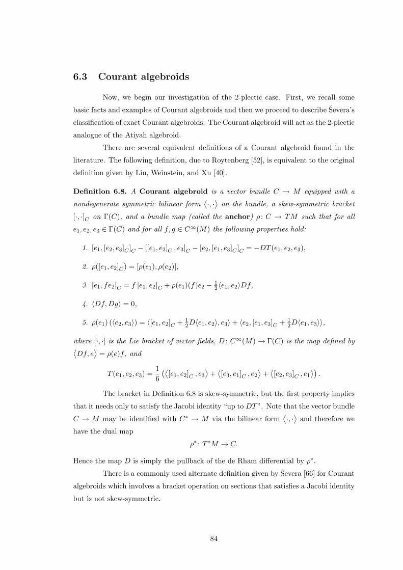
6.3 Courant algebroids

Now, we begin our investigation of the 2-plectic case. First, we recall some

basic facts and examples of Courant algebroids and then we proceed to describe Severa’s

classification of exact Courant algebroids. The Courant algebroid will act as the 2-plectic

analogue of the Atiyah algebroid.

There are several equivalent definitions of a Courant algebroid found in the

literature. The following definition, due to Roytenberg [52], is equivalent to the original

definition given by Liu, Weinstein, and Xu [40].

Definition 6.8. A Courant algebroid is a vector bundle C → M equipped with a

nondegenerate symmetric bilinear form⟨·, ·⟩

on the bundle, a skew-symmetric bracket

[·, ·]C on Γ(C), and a bundle map (called the anchor) ρ : C → TM such that for all

e1, e2, e3 ∈ Γ(C) and for all f, g ∈ C∞(M) the following properties hold:

1. [e1, [e2, e3]C ]C − [[e1, e2]C , e3]C − [e2, [e1, e3]C ]C = −DT (e1, e2, e3),

2. ρ([e1, e2]C) = [ρ(e1), ρ(e2)],

3. [e1, fe2]C = f [e1, e2]C + ρ(e1)(f)e2 − 12〈e1, e2〉Df ,

4. 〈Df,Dg〉 = 0,

5. ρ(e1) (〈e2, e3〉) = 〈[e1, e2]C + 12D〈e1, e2〉, e3〉+ 〈e2, [e1, e3]C + 1

2D〈e1, e3〉〉,

where [·, ·] is the Lie bracket of vector fields, D : C∞(M)→ Γ(C) is the map defined by⟨Df, e

⟩= ρ(e)f , and

T (e1, e2, e3) =16(⟨

[e1, e2]C , e3

⟩+⟨[e3, e1]C , e2

⟩+⟨[e2, e3]C , e1

⟩).

The bracket in Definition 6.8 is skew-symmetric, but the first property implies

that it needs only to satisfy the Jacobi identity “up to DT”. Note that the vector bundle

C → M may be identified with C∗ → M via the bilinear form⟨·, ·⟩

and therefore we

have the dual map

ρ∗ : T ∗M → C.

Hence the map D is simply the pullback of the de Rham differential by ρ∗.

There is a commonly used alternate definition given by Severa [66] for Courant

algebroids which involves a bracket operation on sections that satisfies a Jacobi identity

but is not skew-symmetric.

84

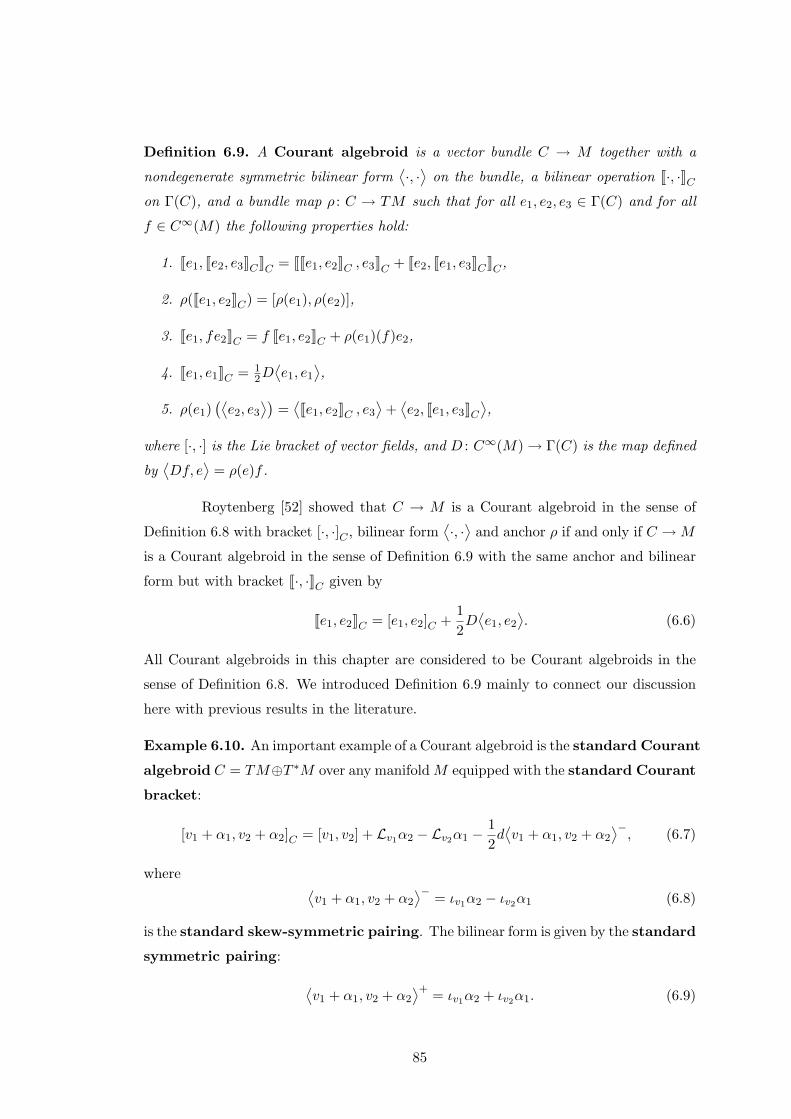
Definition 6.9. A Courant algebroid is a vector bundle C → M together with a

nondegenerate symmetric bilinear form⟨·, ·⟩

on the bundle, a bilinear operation J·, ·KCon Γ(C), and a bundle map ρ : C → TM such that for all e1, e2, e3 ∈ Γ(C) and for all

f ∈ C∞(M) the following properties hold:

1. Je1, Je2, e3KCKC = JJe1, e2KC , e3KC + Je2, Je1, e3KCKC ,

2. ρ(Je1, e2KC) = [ρ(e1), ρ(e2)],

3. Je1, fe2KC = f Je1, e2KC + ρ(e1)(f)e2,

4. Je1, e1KC = 12D⟨e1, e1

⟩,

5. ρ(e1)(⟨e2, e3

⟩)=⟨Je1, e2KC , e3

⟩+⟨e2, Je1, e3KC

⟩,

where [·, ·] is the Lie bracket of vector fields, and D : C∞(M)→ Γ(C) is the map defined

by⟨Df, e

⟩= ρ(e)f .

Roytenberg [52] showed that C → M is a Courant algebroid in the sense of

Definition 6.8 with bracket [·, ·]C , bilinear form⟨·, ·⟩

and anchor ρ if and only if C →M

is a Courant algebroid in the sense of Definition 6.9 with the same anchor and bilinear

form but with bracket J·, ·KC given by

Je1, e2KC = [e1, e2]C +12D⟨e1, e2

⟩. (6.6)

All Courant algebroids in this chapter are considered to be Courant algebroids in the

sense of Definition 6.8. We introduced Definition 6.9 mainly to connect our discussion

here with previous results in the literature.

Example 6.10. An important example of a Courant algebroid is the standard Courant

algebroid C = TM⊕T ∗M over any manifold M equipped with the standard Courant

bracket:

[v1 + α1, v2 + α2]C = [v1, v2] + Lv1α2 − Lv2α1 −12d⟨v1 + α1, v2 + α2

⟩−, (6.7)

where ⟨v1 + α1, v2 + α2

⟩− = ιv1α2 − ιv2α1 (6.8)

is the standard skew-symmetric pairing. The bilinear form is given by the standard

symmetric pairing:

⟨v1 + α1, v2 + α2

⟩+ = ιv1α2 + ιv2α1. (6.9)

85

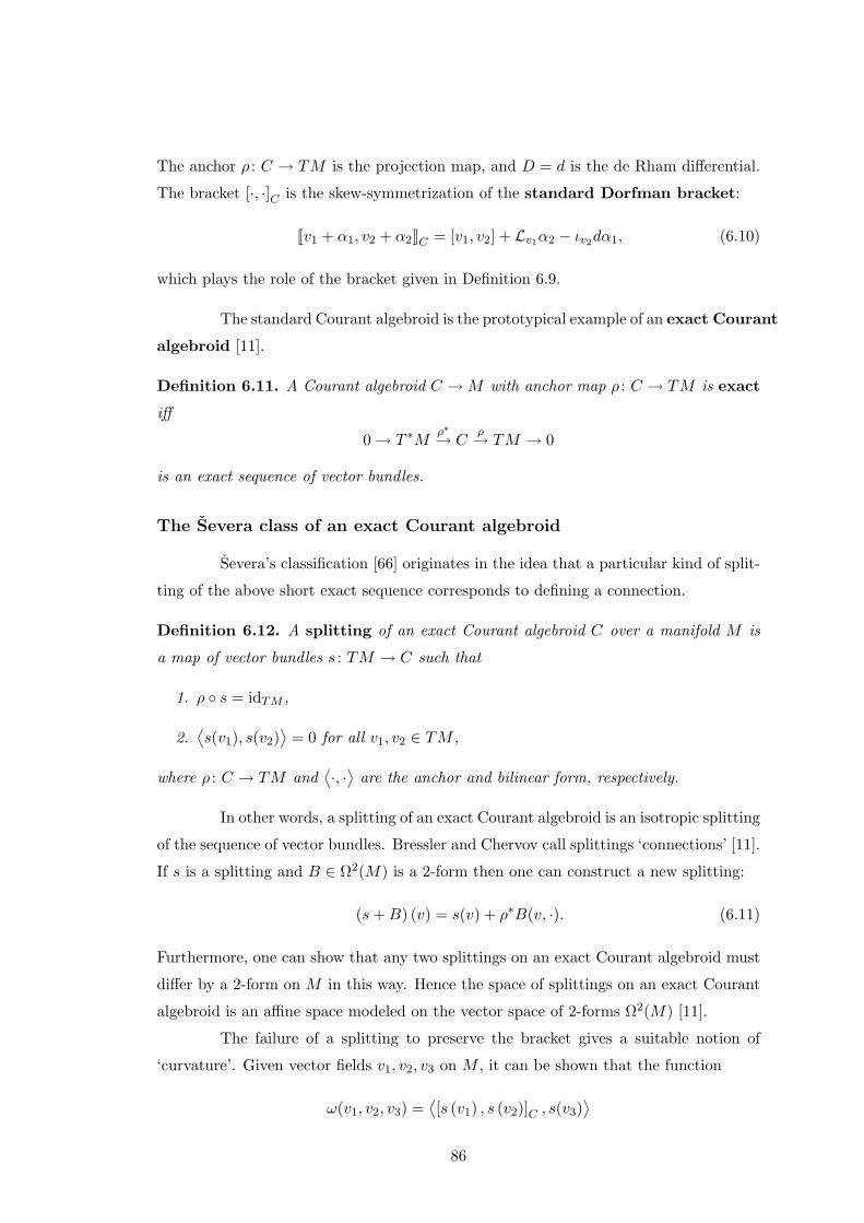
The anchor ρ : C → TM is the projection map, and D = d is the de Rham differential.

The bracket [·, ·]C is the skew-symmetrization of the standard Dorfman bracket:

Jv1 + α1, v2 + α2KC = [v1, v2] + Lv1α2 − ιv2dα1, (6.10)

which plays the role of the bracket given in Definition 6.9.

The standard Courant algebroid is the prototypical example of an exact Courant

algebroid [11].

Definition 6.11. A Courant algebroid C →M with anchor map ρ : C → TM is exact

iff

0→ T ∗Mρ∗→ C

ρ→ TM → 0

is an exact sequence of vector bundles.

The Severa class of an exact Courant algebroid

Severa’s classification [66] originates in the idea that a particular kind of split-

ting of the above short exact sequence corresponds to defining a connection.

Definition 6.12. A splitting of an exact Courant algebroid C over a manifold M is

a map of vector bundles s : TM → C such that

1. ρ s = idTM ,

2.⟨s(v1), s(v2)

⟩= 0 for all v1, v2 ∈ TM ,

where ρ : C → TM and⟨·, ·⟩

are the anchor and bilinear form, respectively.

In other words, a splitting of an exact Courant algebroid is an isotropic splitting

of the sequence of vector bundles. Bressler and Chervov call splittings ‘connections’ [11].

If s is a splitting and B ∈ Ω2(M) is a 2-form then one can construct a new splitting:

(s+B) (v) = s(v) + ρ∗B(v, ·). (6.11)

Furthermore, one can show that any two splittings on an exact Courant algebroid must

differ by a 2-form on M in this way. Hence the space of splittings on an exact Courant

algebroid is an affine space modeled on the vector space of 2-forms Ω2(M) [11].

The failure of a splitting to preserve the bracket gives a suitable notion of

‘curvature’. Given vector fields v1, v2, v3 on M , it can be shown that the function

ω(v1, v2, v3) =⟨[s (v1) , s (v2)]C , s(v3)

⟩86

defines a closed 3-form on M [11]. This is the curvature 3-form of an exact Courant

algebroid over M . It gives a well-defined cohomology class in H3DR(M), independent of

the choice of splitting.

Definition 6.13 ([26]). The Severa class of an exact Courant algebroid with bracket

[·, ·]C and bilinear form⟨·, ·⟩

is the cohomology class [−ω] ∈ H3DR(M), where

ω(v1, v2, v3) =⟨[s (v1) , s (v2)]C , s(v3)

⟩.

6.4 Courant algebroids and 2-plectic geometry

In this section, we describe a relationship between Courant algebroids and 2-

plectic manifolds which can be understood as the higher analogue of the relationship

between Atiyah algebroids and symplectic manifolds.

We begin by recalling how to explicitly construct an exact Courant algebroid

with Severa class [ω]. This is the 3-form version of the construction that gives a transitive

Lie algebroid over a pre-symplectic manifold, which was previously discussed in Sec. 6.2.

The approach given here is essentially identical to those given by Gualtieri [26], Hitchin

[29], and Severa [66] .

Let (M,ω) be a manifold equipped with a closed 3-form. A trivialization of ω is

an open coverUi of M equipped with 2-forms Bi ∈ Ω2(Ui), and 1-forms Aij ∈ Ω1(Uij)

on intersections such that

ω|Ui = dBi

(Bj −Bi)|Uij = dAij .(6.12)

Given such a trivialization, over each open set Ui consider the bundle Ci = TUi⊕T ∗Ui →Ui equipped with the standard pairing⟨

v1 + α1, v2 + α2

⟩+

i= ιv1α2 + ιv2α1, (6.13)

v1, v2 ∈ X(Ui), α1, α2 ∈ Ω1(Ui), which has signature (n, n). On double intersections, it

is easy to see that⟨v1 + ιv1dAij + α1, v2 + ιv2dAij + α2

⟩+

i=⟨v1 + α1, v2 + α2

⟩+

i.

Hence the 2-forms dAij generate transition functions

Gij : Uij → SO(n, n),

Gij(x) =

1 0

dAij |x 1

,

87

which satisfy the cocycle conditions on Uijk by virtue of Eq. 6.12. Therefore, we have

over M the vector bundle

C =∐x∈M

TxUi ⊕ T ∗xUi/ ∼,

equipped with a bilinear form denoted as⟨·, ·⟩+. C sits in the exact sequence

0→ T ∗M→ C

ρ→ TM → 0,

where the anchor ρ is induced by the projection T ∗Ui⊕TUi → TUi, and is the inclusion.

The 2-forms Bi induce a bundle map s : TM → C

s(vx) = vx −Bi(vx) if x ∈ Ui, (6.14)

It follows from Eq. 6.12 that s is well-defined when x ∈ Uij . It is easy to see that this

map is an isotropic splitting (Def. 6.12). Hence every section e ∈ Γ(C) can be uniquely

expressed as

e = s(v) + α,

for some v ∈ X(M) and α ∈ Ω1(M). As before, we use s to also denote the map

Γ(s) : X(M)→ Γ(C). The anchor map is just

ρ(s(v) + α

)= v. (6.15)

Given sections s(v1) +α1, s(v2) +α2 ∈ Γ(C), a local calculation using Eq. 6.14

gives ⟨s(v1) + α1, s(v2) + α2

⟩+ = ιv1α2 − ιv1ιv2Bi + ιv2α1 − ιv2ιv1Bi

=⟨v1 + α1, v2 + α2

⟩+.

(6.16)

The above equality holds, in fact, for any splitting s′ : TM → C, since s− s′ is a 2-form

on M and therefore skew-symmetric. The bracket on Γ(C) is defined over the open set

Ui by:

[s(v1) + α1, s(v2) + α2]C |Ui = [s(v1) + α1, s(v2) + α2]i

where [·, ·]i is the standard Courant bracket (6.7) on Ci. Since the 2-forms dAij are

closed, it follows by direct computation that on double intersections Uij :

[Gij(v1 + α1), Gij(v2 + α2)]i = Gij([v1 + α1, v2 + α2]i

).

Hence the bracket [·, ·]C is indeed globally well-defined. Using the local definition of the

bracket and the splitting, as well as the fact that dBi = ω, it is easy to show that

[s(v1) + α1, s(v2) + α2]C = s([v1, v2]

)+ Lv1α2 − Lv2α1

− 12d⟨v1 + α1, v2 + α2

⟩− − ιv2ιv1ω. (6.17)

88

The bracket [·, ·]C is called the twisted Courant bracket. A analogous construction

using the standard Dorfman bracket (6.10) on Ci gives the twisted Dorfman bracket:

Js(v1) + α1, s(v2) + α2KC = s([v1, v2]

)+ Lv1α2 − ιv2dα1 − ιv2ιv1ω. (6.18)

These brackets were studied in detail by Severa and Weinstein [61, 66].

It is straightforward to check that C → M equipped with the aforementioned

bilinear form, anchor, and bracket [·, ·]C is an exact Courant algebroid (Definition 6.8).

Just as in Lie algebroid case, the construction of C is independent of the choice of

trivialization up to a splitting-preserving isomorphism.

A direct calculation shows that

−ω(v1, v2, v3) =⟨[s (v1) , s (v2)]C , s(v3)

⟩+.

Hence, the Courant algebroid C has Severa class [ω]. Of course, we are interested in the

special case when ω is a 2-plectic structure. We summarize the above discussion with

the following proposition:

Proposition 6.14. Let (M,ω) be a 2-plectic manifold. Up to isomorphism, there exists

a unique exact Courant algebroid C over M , with bilinear form⟨·, ·⟩+, anchor map ρ,

and bracket [·, ·]C given in Eqs. 6.13, 6.15, and 6.17, respectively, and equipped with a

splitting whose curvature is −ω.

Lie 2-algebras from Courant algebroids

Next, we describe how a Courant algebroid gives a Lie 2-algebra. From here

on, we shall describe a Lie 2-algebra using the terminology given in Prop. 3.10, i.e. as a

2-term chain complex, equipped with a bracket and a Jacobiator.

Recall that the space of global sections of a transitive Lie algebroid associated

to a closed 2-form gives a Lie algebra. As we shall see, the global sections of a Courant

algebroid form a Lie 2-algebra. Given any Courant algebroid C →M with bilinear form⟨·, ·⟩, bracket [·, ·]C , and anchor ρ : C → TM , one can construct a 2-term chain complex

L = C∞(M) D→ Γ(C),

with differential D = ρ∗d where d is the de Rham differential. The bracket [·, ·]C on

global sections can be extended to a chain map [·, ·] : L⊗ L→ L. If e1, e2 are degree 0

chains then [e1, e2] is the original bracket. If e is a degree 0 chain and f, g are degree 1

chains, then we define:

[e, f ] = − [f, e] =12⟨e,Df

⟩[f, g] = 0.

89

It was shown by Roytenberg and Weinstein [55] that this extended bracket gives a

L∞-algebra. Roytenberg’s later work [53, 54] implies that a brutal truncation of this

L∞-algebra is a Lie 2-algebra whose underlying complex is L. For the Courant algebroid

C associated to a 2-plectic manifold, their result implies:

Theorem 6.15. If C is the exact Courant algebroid given in Proposition 6.14 then there

is a Lie 2-algebra L∞(C) = (L, [·, ·], J) where:

• L0 = Γ(C),

• L1 = C∞(M),

• the differential L1d→ L0 is the de Rham differential

• the bracket [·, ·] is

[e1, e2] = [e1, e2]C in degree 0

and

[e, f ] = −[f, e] =12⟨e, df

⟩+ in degree 1,

• the Jacobiator is the linear map J : Γ(C)⊗ Γ(C)⊗ Γ(C)→ C∞(M) defined by

J(e1, e2, e3) = −T (e1, e2, e3)

= −16

(⟨[e1, e2]C , e3

⟩+ +⟨[e3, e1]C , e2

⟩+

+⟨[e2, e3]C , e1

⟩+).

More precisely, the theorem follows from Example 5.4 of [54] and Section 4 of

[53]. On the other hand, the original construction of Roytenberg and Weinstein gives a

L∞-algebra on the complex:

0→ kerD ι→ C∞(M) D→ Γ(C),

with trivial structure maps ln for n > 3. Moreover, the map l2 (corresponding to the

bracket [·, ·] given above) is trivial in degree > 1 and the map l3 (corresponding to the

Jacobiator J) is trivial in degree > 0. Hence these maps induce the above Lie 2-algebra

structure on C∞(M) D→ Γ(C).

The algebraic relationship between 2-plectic and Courant

Associated to any 2-plectic manifold (M,ω), is a Lie 2-algebra L∞(M,ω) (Thm.

3.14). In Prop. 3.15, we described this Lie 2-algebra as a 2-term chain complex L =

(L1d−→ L0) equipped with a bracket [·, ·] and Jacobiator J where:

90

• L0 = Ω1Ham (M) is the space of Hamiltonian 1-forms,

• L1 = C∞(M),

• the differential L1d→ L0 is the de Rham differential,

• the bracket [·, ·] is α, β = ω(vα, vβ, ·) in degree 0 and trivial otherwise,

• the Jacobiator is given by the linear map J : Ω1Ham(M)⊗Ω1

Ham(M)⊗Ω1Ham(M)→

C∞, where J(α, β, γ) = ω(vγ , vβ, vα).

Also associated to (M,ω), is the exact Courant algebroid (C, [·, ·]C ,⟨·, ·⟩+, ρ) described

in Prop. 6.14, equipped with a splitting s : TM → C whose curvature is −ω. From this

Courant algebroid, we obtain the Lie 2-algebra L∞(C) described in Thm. 6.15.

We now describe the relationship between L∞(M,ω) and L∞(C). We under-

stand this as the 2-plectic analogue of the relationship described in Sec. 6.2 between the

Poisson algebra of a symplectic manifold and the Lie algebra associated to the transitive

Lie algebroid over the manifold.

Theorem 6.16. Let (M,ω) be a 2-plectic manifold and let C be its corresponding

Courant algebroid. Let L∞(M,ω) and L∞(C) be the Lie 2-algebras corresponding to

(M,ω) and C, respectively. There exists a morphism of Lie 2-algebras embedding L∞(M,ω)

into L∞(C).

Before we prove the theorem, we introduce some technical lemmas to ease the

calculations. Recall from Eq. 6.8 that the formula for the standard skew-symmetric

pairing on X(M)⊕ Ω1(M):

⟨v1 + α1, v2 + α2

⟩− = ιv1α2 − ιv2α1.

In what follows, by the symbol “c.p” we mean cyclic permutations of the symbols α, β, γ.

Lemma 6.17. If α, β ∈ Ω1Ham(M) with corresponding Hamiltonian vector fields vα, vβ,

then Lvαβ = α, β+ dιvαβ.

Proof. Since Lv = ιvd+ dιv,

Lvαβ = ιvαdβ + dιvαβ = −ιvαιvβω + dιvαβ = α, β+ dιvαβ.

91

Lemma 6.18. If α, β, γ ∈ Ω1Ham(M) with corresponding Hamiltonian vector fields

vα, vβ, vγ, then

ι[vα,vβ ]γ + c.p = −3ιvαιvβ ιvγω + ιvαd⟨vβ + β, vγ + γ

⟩−+ ιvγd

⟨vα + α, vβ + β

⟩− + ιvβd⟨vγ + γ, vα + α

⟩−.

Proof. The identity ι[vα,vβ ] = Lvαιvβ − ιvβLvα and Lemma 6.17 imply:

ι[vα,vβ ]γ = L vα ιvβγ − ιvβL vα γ

= L vα ιvβγ − ιvβ (α, γ+ dιvαγ)

= ιvαdιvβγ − ιvβ ιvγ ιvαω − ιvβdιvαγ,

where the last equality follows from the definition of the bracket.

Therefore we have:

ι[vγ ,vα]β = ιvγdιvαβ − ιvαιvβ ιvγω − ιvαdιvγβ,

ι[vβ ,vγ ]α = ιvβdιvγα− ιvγ ιvαιvβω − ιvγdιvβα,

and Eq. 6.8 implies

ιvαdιvβγ − ιvαdιvγβ = ιvαd⟨vβ + β, vγ + γ

⟩−.

The statement then follows.

Lemma 6.19. If α, β ∈ Ω1Ham(M) with corresponding Hamiltonian vector fields vα, vβ,

then

L vα β − L vβ α = 2 α, β+ d⟨vα + α, vβ + β

⟩−.

Proof. Follows immediately from Lemma 6.17 and Eq. 6.8.

We have all we need to give a proof of Thm. 6.16.

Proof of Theorem 6.16. Let

L = C∞(M) d→ Ω1Ham(M),

[·, ·]L : L⊗ L→ L,

JL : L⊗ L⊗ L→ L

denote the underlying chain complex, bracket, and Jacobiator of the Lie 2-algebra

L∞(M,ω). Similarly,

L′ = C∞(M) d→ Γ(C),

[·, ·]L′ : L′ ⊗ L′ → L′,

JL′ : L′ ⊗ L′ ⊗ L′ → L′

92

denotes the underlying chain complex, bracket, and Jacobiator of the Lie 2-algebra

L∞(C).

We construct a Lie 2-algebra morphism from L∞(M,ω) to L∞(C). Recall from

Def. 3.11, that such a morphism consists of

• a chain map φ : L→ L′, and

• a chain homotopy Φ: L⊗ L→ L′ from the chain map

L⊗ L → L′

x⊗ y 7−→ φ ([x, y])

to the chain mapL⊗ L → L′

x⊗ y 7−→ [φ(x), φ(y)]′ ,

such that the following equation holds:

φ1(J(x, y, z))− J ′(φ0(x), φ0(y), φ0(z)) =

Φ(x, [y, z])− Φ([x, y], z)− Φ(y, [x, z])− [Φ(x, y), φ0(z)]′

+[φ0(x),Φ(y, z)]′ − [φ0(y),Φ(x, z)]′.

(6.19)

Let s : TM → C be the splitting. Let φ0 : Ω1Ham(M)→ Γ(C) be given by

φ0(α) = s(vα) + α,

where vα is the Hamiltonian vector field corresponding to α. Let φ1 : C∞(M)→ C∞(M)

be the identity. Then φ : L → L′ is a chain map, since the Hamiltonian vector field of

an exact 1-form is zero. Let Φ: Ω1Ham(M)⊗ Ω1

Ham(M)→ C∞(M) be given by

Φ(α, β) = −12⟨vα + α, vβ + β

⟩−.

Now we show Φ is a well-defined chain homotopy in the sense of Def. 3.11. We

have

[φ0(α), φ0(β)]L′ = [s(vα) + α, s(vβ) + β]C

= s([vα, vβ]) + Lvαβ − Lvβα− ιvβ ιvαω

− 12d⟨vα + α, vβ + β

⟩−= s([vα, vβ]) + α, β+

12d⟨vα + α, vβ + β

⟩−= s([vα, vβ]) + [α, β]L − dΦ(α, β).

(6.20)

93

The second line above is just the definition of the twisted Courant bracket (Eq. 6.17),

while the second to last line follows from Lemma 6.19 and Def. 3.3 of the bracket ·, ·.By Prop. 3.4, the Hamiltonian vector field of α, β is [vα, vβ]. Hence we have:

φ0([α, β]L)− [φ0(α), φ0(β)]L′ = dΦ(α, β).

In degree 1, the bracket [·, ·]L is trivial. It follows from the definition of [·, ·]L′that

φ1([α, f ]L)− [φ0(α), φ1(f)]L′ = −12⟨s(vα) + α, df

⟩+.

From Eq. 6.16, we have⟨s(vα) + α, df

⟩+ =⟨s(vα) + α, s(0) + df

⟩+ = ιvαdf.

Therefore

φ1([α, f ]L)− [φ0(α), φ1(f)]L′ = Φ(α, df),

and similarly

φ1([f, α]L)− [φ1(f), φ0(α)]L′ = Φ(df, α).

Therefore Φ is a chain homotopy.

It remains to show the coherence condition (Eq. 6.19 in Definition 3.11) is

satisfied. First we rewrite the Jacobiator JL′ using the second to last line of (6.20):

JL′(φ0(α), φ0(β), φ0(γ)) = −16⟨[φ0(α), φ0(β)]L′ , φ0(γ)

⟩+ + c.p

= −16⟨s([vα, vβ]) + α, β − dΦ(α, β), s(vγ) + γ

⟩+

+ c.p .

From the definition of the bracket ·, · and the symmetric pairing, we have

JL′(φ0(α), φ0(β), φ0(γ)) = −12ιvγ ιvβ ιvαω −

16(ι[vα,vβ ]γ − ιvγdΦ(α, β) + c.p

). (6.21)

Lemma 6.18 implies

ι[vα,vβ ]γ + c.p = −3ιvαιvβ ιvγω −(2ιvγdΦ(α, β) + c.p

), (6.22)

so Eq. 6.21 becomes

JL′(φ0(α), φ0(β), φ0(γ)) = ιvαιvβ ιvγω +(1

2ιvγdΦ(α, β) + c.p

).

By definition, JL(α, β, γ) = ιvαιvβ ιvγω. Therefore, in this case, the left-hand side of Eq.

6.19 is

φ1(JL(α, β, γ))− JL′(φ0(α), φ0(β), φ0(γ)) = −12ιvγdΦ(α, β) + c.p . (6.23)

94

Since the brackets and homotopy Φ are skew-symmetric, the right-hand side

of Eq. 6.19 can be rewritten as:

(Φ(α, [β, γ]L) + c.p

)−([Φ(α, β), φ0(γ)]L′ + c.p

). (6.24)

Consider the first term in Eq. 6.24. The Hamiltonian vector field corresponding to

[β, γ]L = β, γ is [vβ, vγ ]. Therefore the definition of Φ implies

Φ(α, [β, γ]L) + c.p = −32ιvγ ιvβ ιvαω +

12(ι[vβ ,vγ ]α+ c.p

).

It then follows from Lemma 6.18 (see Eq. 6.22) that

Φ(α, [β, γ]L) + c.p = −ιvγdΦ(α, β) + c.p .

By definition of the bracket [·, ·]L′ , the second term in Eq. 6.24 can be written as

[Φ(α, β), φ0(γ)]L′ + c.p = −12ιvγdΦ(α, β) + c.p .

Hence the coherence condition:

φ1(JL(α, β, γ))− JL′(φ0(α), φ0(β), φ0(γ)) = Φ(α, [β, γ]L)− [Φ(α, β), φ0(γ)]L′ + c.p

is satisfied, and (φ,Φ): L∞(M,ω)→ L∞(C) is a morphism of Lie 2-algebras.

We now focus on a particular sub-Lie 2-algebra of L∞(C). The following

definition is due to Severa [66] and is a generalization of Def. 6.5:

Definition 6.20. Let C be the exact Courant algebroid given in Prop. 6.14 equipped

with a splitting s : TM → C. We say a section e = s(v) + α preserves the splitting

iff ∀v′ ∈ X(M)qe, s(v′)

yC

= s([v, v′]).

The subspace of sections that preserve the splitting is denoted as Γ(C)s.

Note that the twisted Dorfman bracket is used in the above definition rather

than the twisted Courant bracket. Since it satisfies the Jacobi identity, it gives a ‘strict’

adjoint action on sections of C. The 2-plectic analogue of Proposition 6.6 is:

Proposition 6.21. If C is the exact Courant algebroid given in Proposition 6.14 equipped

with the splitting s : TM → C, then there is a Lie 2-algebra L∞(C)s = (L, [·, ·], J) where:

• L0 = Γ(C)s,

• L1 = C∞(M),

95

• the differential L1d→ L0 is the de Rham differential

• the bracket [·, ·] is

[e1, e2] = [e1, e2]C in degree 0

and

[e, f ] = −[f, e] =12⟨e, df

⟩+ in degree 1,

• the Jacobiator is the linear map J : Γ(C)s ⊗ Γ(C)s ⊗ Γ(C)s → C∞(M) defined by

J(e1, e2, e3) = −T (e1, e2, e3)

= −16

(⟨[e1, e2]C , e3

⟩+ +⟨[e3, e1]C , e2

⟩+

+⟨[e2, e3]C , e1

⟩+).

Proof. Let v′ be a vector field on M . By the definition of the twisted Dorfman bracket

(Eq. 6.18), it follows that Jdf, s(v′)KC = 0 ∀f ∈ C∞(M). Hence the complex L is well-

defined. We now show that Γs(C) is closed under the twisted Courant bracket. Suppose

e1 and e2 are sections preserving the splitting. Let ei = s(vi) + αi. Since the twisted

Dorfman bracket and the Lie bracket of vector fields satisfy the Jacobi identity, we have:

qJe1, e2KC , s(v

′)yC

= s([[v1, v2], v′]).

From Eq. 6.6, we have the identity:

[e1, e2]C = Je1, e2KC −12d⟨e1, e2

⟩+.

Therefore:

q[e1, e2]C , s(v

′)yC

=qJe1, e2KC , s(v

′)yC− 1

2

rd⟨e1, e2

⟩+, s(v′)

z

C

= s([[v1, v2], v′]).

It follows from Theorem 6.15 that the Lie 2-algebra axioms are satisfied.

This next result is essentially a corollary of Thm. 6.16. However, it is important

since it is the 2-plectic analogue of Prop. 6.7.

Theorem 6.22. L∞(M,ω) and L∞(C)s are isomorphic as Lie 2-algebras.

Proof. Recall that in Theorem 6.16 we constructed a morphism of Lie 2-algebras given

by a chain map φ : L∞(M,ω)→ L∞(C):

φ0(α) = s(vα) + α, φ1 = id,

96

and a homotopy Φ: Ω1Ham(M)⊗ Ω1

Ham(M)→ C∞(M):

Φ(α, β) = −12⟨vα + α, vβ + β

⟩−.

Let v′ ∈ X(M) and e = s(v) + α. By definition of the twisted Dorfman bracket,

Je, s(v′)KC = s[v, v′] if and only if ιv′(dα+ ιvω

)= 0. Hence a section of C preserves the

splitting if and only if it lies in the image of the chain map φ. Since this map is also

injective, the statement follows.

Theorem 6.22 suggests that we interpret the Lie 2-algebra L∞(C)s as the pre-

quantization of the Lie 2-algebra of “observables” L∞(M,ω). Clearly, these results

further support the idea that exact Courant algebroids play the role of higher Atiyah

algebroids [11, 26]. However, interpreting L∞(C)s as ‘operators’ or as infinitesimal sym-

metries of a U(1)-gerbe with 2-connection is still a work in progress. It is likely that

significant progress would be made by solving the larger problem of how to integrate an

exact Courant algebroid to a Lie 2-groupoid.

6.5 Central extensions of Lie 2-algebras

In this section, we constructing the 2-plectic version of the Kostant-Souriau

central extension, which we discussed in Sec. 6.2. First some preliminary definitions:

Definition 6.23. A Lie 2-algebra (L, [·, ·], J) is trivial iff L1 = 0.

Any Lie algebra g gives a trivial Lie 2-algebra whose underlying complex is

0→ g.

In particular, the Lie algebra of Hamiltonian vector fields XHam(M) is a trivial Lie

2-algebra.

Definition 6.24. A Lie 2-algebra (L, [·, ·], J) is abelian iff [·, ·] = 0 and J = 0.

Hence an abelian Lie 2-algebra is just a 2-term chain complex.

Definition 6.25. If L, L′, and L′′ are Lie 2-algebras, then L′ is a strict extension of

L′′ by L iff there exists Lie 2-algebra morphisms

(φ,Φ): L→ L′, (φ′,Φ′) : L′ → L′′

such that the chain maps φ, φ′ give a short exact sequence of the underlying chain

complexes

Lφ→ L′

φ′→ L′′.

97

We say L′ is a strict central extension of L′′ iff L′ is an extension of L′′ by L and[imφ,L′

]′ = 0.

Remark 6.26. These definitions will be sufficient for our work here. However, they

are, in general, too strict. For example, one can have homotopies between morphisms

between Lie 2-algebras, and therefore we should consider sequences that are only exact

up to homotopy as “exact”. Fully weak extensions for degree-wise finite-dimensional Lie

n-algebras have recently been described as particular homotopy pushouts in the closed

model category of differential graded (dg) algebras [59]. The opposite of this model

structure is taken to be, by definition, a presentation of the (∞, 1)-category of degree-

wise finite-dimensional L∞-algebras. For infinite-dimensional Lie n-algebras, such as

the ones we consider here, it is likely that one can find a suitable definition in a similar

manner by using a closed model category structure on the category of dg co-algebras.

We would like to understand how L∞(M,ω) is a central extension of XHam(M)

as a Lie 2-algebra. Our first two results are quite general and hold for any 2-plectic

manifold (M,ω).

Proposition 6.27. If (M,ω) is a 2-plectic manifold, then the Lie 2-algebra L∞(M,ω)

is a central extension of the trivial Lie 2-algebra XHam(M) by the abelian Lie 2-algebra

C∞(M) d→ Ω1cl(M),

consisting of smooth functions and closed 1-forms.

Proof. Consider the following short exact sequence of complexes:

Ω1cl(M)

// Ω1Ham(M)

p // XHam(M)

C∞(M)

d

OO

id // C∞(M)

d

OO

// 0

OO(6.25)

The map : Ω1cl(M)→ Ω1

Ham(M) is the inclusion, and

p : Ω1Ham(M)→ XHam(M), p(α) = vα

takes a Hamiltonian 1-form to its corresponding vector field. It follows from Prop.

3.4 that p preserves the bracket. In fact, all of the horizontal chain maps give strict

Lie 2-algebra morphisms (i.e. all homotopies are trivial). The Hamiltonian vector field

corresponding to a closed 1-form is zero. Thus, if α is closed, then for all β ∈ Ω1Ham(M)

we have [α, β]L∞(M,ω) = α, β = 0. Hence L∞(M,ω) is a central extension of XHam(M).

98

Proposition 6.28. Let (M,ω) be a 2-plectic manifold. Given x ∈ M , there is a Lie

2-algebra L∞(XHam(M), x) = (L, [·, ·], Jx) where

• L0 = XHam(M),

• L1 = R,

• the differential L1d→ L0 is trivial (d = 0),

• the bracket [·, ·] is the Lie bracket on XHam(M) in degree 0 and trivial in all other

degrees

• the Jacobiator is the linear map

Jx : XHam(M)⊗ XHam(M)⊗ XHam(M)→ R

defined by

Jx(v1, v2, v3) = ιv1ιv2ιv3ω|x.

Moreover, Jx is a 3-cocycle in the Chevalley-Eilenberg cochain complex

Hom(Λ•XHam(M),R).

Proof. We have a bracket defined on a complex with trivial differential that satisfies

the Jacobi identity “on the nose”. Hence to show L∞(XHam(M), x) is a Lie 2-algebra,

it sufficient to show that the Jacobiator Jx(v1, v2, v3) satisfies Eq. 3.10 in Def. 3.10 for

x ∈ M . This follows immediately from Thm. 3.15. The classification theorem of Baez

and Crans (Thm. 55 in [4]) implies that Jx satisfying Eq. 3.10 in the definition of a Lie 2-

algebra is equivalent to Jx being a 3-cocycle with values in the trivial representation.

Recall that in the symplectic case, if the manifold is connected, then the Poisson

algebra is a central extension of the Hamiltonian vector fields by the Lie algebra u(1) ∼=R. The categorified analog of the Lie algebra u(1) is the abelian Lie 2-algebra bu(1)

whose underlying chain complex is simply

R→ 0.

It is natural to suspect that, under suitable topological conditions, the abelian Lie

algebra C∞(M) d→ Ω1cl(M) introduced in Prop. 6.27 is related to bu(1).

Let us first assume that the 2-plectic manifold is connected. Note that the

Jacobiator Jx of the Lie 2-algebra L∞(XHam(M), x) introduced in Prop. 6.28 depends

explicitly on the choice of x ∈M . However, if M is connected, then the cohomology class

Jx represents as a 3-cocycle does not depend on x. This fact has important implications

for L∞(XHam(M), x):

99

Proposition 6.29. If (M,ω) is a connected 2-plectic manifold and Jx is the 3-cocycle

given in Prop. 6.28, then the cohomology class [Jx] ∈ H3CE(XHam(M),R) is independent

of the choice of x ∈ M . Moreover, given any other point y ∈ M , the Lie 2-algebras

L∞(XHam(M), x) and L∞(XHam(M), y) are quasi-isomorphic.

Proof. To prove that [Jx] is independent of x, we use a construction similar to the proof

of Prop. 4.1 in [12]. The Chevalley-Eilenberg differential

δ : Hom(ΛnXHam(M),R)→ Hom(Λn+1XHam(M),R)

is defined by

(δc)(v1, . . . , vn+1) =∑

1≤i<j≤n(−1)i+jc([vi, vj ], v1, · · · , vi, · · · , vj , . . . , vn+1).

Note that if c is an arbitrary 2-cochain then

(δc)(vα, vβ, vγ) = −c([vα, vβ], vγ) + c([vα, vγ ], vβ)− c([vβ, vγ ], vα).

Now let y ∈ M . Let Γ: [0, 1] → M be a path from x to y. Given vα, vβ ∈ XHam(M),

define

c(vα, vβ) =∫

Γω(vα, vβ, ·).

Clearly, c is a 2-cochain. We claim

Jy(vα, vβ, vγ)− Jx(vα, vβ, vγ) = (δc)(vα, vβ, vγ)

The failure of ·, · to satisfy the Jacobi identity implies

dιvαιvβ ιvγω = α, β, γ − α, β , γ − β, α, γ ,

and, from the definition of ·, ·, we have

dιvαιvβ ιvγω = −ω([vα, vβ], vγ , ·) + ω([vα, vγ ], vβ, ·)− ω([vβ, vγ ], vα, ·).

Integrating both sides of the above equation gives∫Γdιvαιvβ ιvγω = Jy(vα, vβ, vγ)− Jx(vα, vβ, vγ)

= −∫

Γω([vα, vβ], vγ , ·) +

∫Γω([vα, vγ ], vβ, ·)−

∫Γω([vβ, vγ ], vα, ·)

= (δc)(vα, vβ, vγ).

It follows from Thm. 57 in Baez and Crans [4] that [Jx] = [Jy] implies L∞(XHam(M), x)

and L∞(XHam(M), y) are quasi-isomorphic (or ‘equivalent’ in their terminology).

100

Now we impose further conditions on our 2-plectic manifold. From here on, we

assume (M,ω) is 1-connected (i.e. connected and simply connected). This is the 2-plectic

analogue of the requirement that the symplectic manifold in Sec. 6.2 be connected. It

will allow us to construct several elementary, yet interesting, quasi-isomorphisms of Lie

2-algebras.

Proposition 6.30. If M is a 1-connected manifold, then the abelian Lie 2-algebra

C∞(M) d→ Ω1cl(M) is quasi-isomorphic to bu(1).

Proof. Let x ∈M . The chain map

C∞(M)

evx

d // Ω1cl(M)

R // 0

is a quasi-isomorphism.

Proposition 6.31. If (M,ω) is a 1-connected 2-plectic manifold and x ∈ M , then the

Lie 2-algebras L∞(M,ω) and L∞(XHam(M), x) are quasi-isomorphic.

Proof. We construct a quasi-isomorphism from L∞(M,ω) to L∞(XHam(M), x). There

is a chain map

C∞(M)

evx

d // Ω1Ham(M)

p

R 0 // XHam(M)

with evx(f) = f(x) and p(α) = vα. Since p preserves the bracket, we take Φ in Def.

3.11 to be the trivial homotopy. Eq. 6.19 holds since:

evx(ω(vγ , vβ, vα)) = Jx(vα, vβ, vγ),

and therefore we have constructed a Lie 2-algebra morphism. Since M is connected, the

homology of the complex C∞(M) d→ Ω1Ham(M) is just R in degree 1 and Ω1

Ham(M)/dC∞(M)

in degree 0. The kernel of the surjective map p is the space of closed 1-forms, which is

dC∞(M) since M is simply connected.

We can summarize the results given in Props. 6.27 6.28 6.30, and 6.31 with the

101

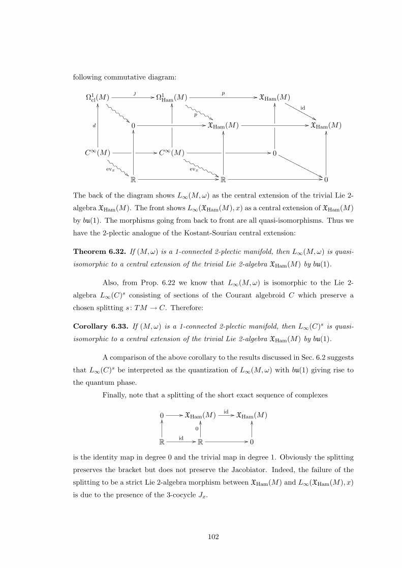
following commutative diagram:

Ω1cl(M)

"""b"b

"b"b

"b"b

// Ω1Ham(M)

p&&&f&f&f&f&f&f

p // XHam(M)id

&&NNNNNNNNNNN

0 // XHam(M) // XHam(M)

C∞(M) //

d

OO

evx###c

#c#c

#c#c

C∞(M)

OO

evx'''g'g'g'g'g'g'g'g

// 0

OO

''OOOOOOOOOOOOOOO

R

OO

// R //

OO

0

OO

The back of the diagram shows L∞(M,ω) as the central extension of the trivial Lie 2-

algebra XHam(M). The front shows L∞(XHam(M), x) as a central extension of XHam(M)

by bu(1). The morphisms going from back to front are all quasi-isomorphisms. Thus we

have the 2-plectic analogue of the Kostant-Souriau central extension:

Theorem 6.32. If (M,ω) is a 1-connected 2-plectic manifold, then L∞(M,ω) is quasi-

isomorphic to a central extension of the trivial Lie 2-algebra XHam(M) by bu(1).

Also, from Prop. 6.22 we know that L∞(M,ω) is isomorphic to the Lie 2-

algebra L∞(C)s consisting of sections of the Courant algebroid C which preserve a

chosen splitting s : TM → C. Therefore:

Corollary 6.33. If (M,ω) is a 1-connected 2-plectic manifold, then L∞(C)s is quasi-

isomorphic to a central extension of the trivial Lie 2-algebra XHam(M) by bu(1).

A comparison of the above corollary to the results discussed in Sec. 6.2 suggests

that L∞(C)s be interpreted as the quantization of L∞(M,ω) with bu(1) giving rise to

the quantum phase.

Finally, note that a splitting of the short exact sequence of complexes

0 // XHam(M) id // XHam(M)

R

OO

id // R

0

OO

// 0

OO

is the identity map in degree 0 and the trivial map in degree 1. Obviously the splitting

preserves the bracket but does not preserve the Jacobiator. Indeed, the failure of the

splitting to be a strict Lie 2-algebra morphism between XHam(M) and L∞(XHam(M), x)

is due to the presence of the 3-cocycle Jx.

102

Summary

Many new results have been given in this chapter, so we conclude with a brief

summary. We defined a prequantized n-plectic manifold to be an integral n-plectic

manifold equipped with Deligne n-cocycle. If (M,ω) is a 0-connected, prequantized

symplectic manifold, then there exists a principal U(1)-bundle over M equipped with a

connection whose curvature is ω, and a corresponding Atiyah algebroid A→M equipped

with a splitting such that the Lie algebra of sections of A which preserve the splitting

is isomorphic to a central extension of the Lie algebra of Hamiltonian vector fields:

u(1)→ C∞(M)→ XHam(M).

This central extension gives a cohomology class in H2CE(XHam(M),R) which can be

represented by the symplectic form evaluated at a point in M .

Analogously, if (M,ω) is a 1-connected, prequantized 2-plectic manifold, then

there exists a U(1)-gerbe over M equipped with a connection and curving whose 3-

curvature is ω, and a corresponding exact Courant algebroid C → M equipped with

a splitting such that the Lie 2-algebra of sections of C which preserve the splitting is

quasi-isomorphic to a central extension of the (trivial) Lie 2-algebra of Hamiltonian

vector fields:

bu(1)→ L∞(XHam(M))→ XHam(M).

This central extension gives a cohomology class in H3CE(XHam(M),R) which can be

represented by the 2-plectic form evaluated at a point in M .

103

Chapter 7

Geometric quantization of

2-plectic manifolds

In the previous chapter, we first considered prequantization for symplectic

manifolds, and then generalized the procedure to 2-plectic manifolds. We were primarily

concerned with prequantizing the algebra of observables, i.e. the Poisson algebra in the

symplectic case, and the Lie 2-algebra of Hamiltonian 1-forms in the 2-plectic case. In

this chapter, we switch our focus from quantizing observables to quantizing states.

Prequantization is a simple and elegant construction. However, numerous ex-

amples in symplectic geometry show that it is only the first step of a two-part process.

Full quantization involves using additional structures in order to construct the correct

space of quantum states. This process was developed over time by considering particular

examples. We suspect that the development of a complete geometric quantization pro-

cedure for 2-plectic manifolds will follow a similar path. In this chapter, we generalize

aspects of the quantization process for symplectic manifolds to the 2-plectic case by us-

ing the higher geometric structures introduced in earlier chapters. The result is a simple

procedure for quantizing 2-plectic manifolds, which we apply to a particular example of

interest. To the best of our knowledge, this is the first geometric quantization procedure

ever developed for such manifolds.

Let us provide some motivation for why additional work beyond prequantiza-

tion is needed in order to obtain the correct quantum states. In the last chapter, we

described a prequantized symplectic manifold as a symplectic manifold equipped with

principal U(1)-bundle with connection. A natural choice for the quantum state space

is the space of square-integrable global sections of the Hermitian line bundle associ-

ated to the principal bundle. This is often called the ‘prequantum Hilbert space’. It

104

comes equipped with an inner product given by integrating the fiber-wise Hermitian

inner product of sections with respect to the symplectic volume form. However, from

the physicist’s point of view, this space is too large to be the space of quantum states

of a physical system.

For example, recall that the cotangent bundle of a manifold is a symplectic

manifold, equipped with its canonical symplectic structure ω =∑

i dpi ∧ dqi. It is, in

fact, an integral symplectic manifold since ω is exact. The sections in the prequantized

Hilbert space locally look like functions f(qi, pi) of 2n variables corresponding to the

“position” coordinates qi of the base manifold and the “momentum” coordinates pi of the

fibers. These functions can have arbitrarily small support, and hence, when interpreted

as wavefunctions on a classical phase space, give probability densities which violate the

Heisenberg uncertainty condition. To get around this problem, one reduces the size of the

Hilbert space by taking the subspace consisting of those sections satisfying ∂f/∂pi = 0.

Hence, the number of “variables” is reduced from 2n to n, by only considering those

sections constant along the fibers.

Consider another example that is perhaps more mathematically interesting.

The coadjoint orbits of the Lie group SU(2) correspond to 2-spheres centered about the

origin in su(2)∗ ∼= R3. Each orbit is a symplectic manifold equipped with what is known

as the ‘KKS symplectic form’. This 2-form is integral if the radius of the sphere is one-

half of a non-negative integer. On each integral orbit, we have the prequantized Hilbert

space, consisting of global square-integrable sections of a Hermitian line bundle. This

Hilbert space is infinite dimensional. However, we can equip the orbit with a complex

structure and consider only holomorphic sections i.e. those sections which locally are

functions f(zi, zi) satisfying ∂f/∂zi = 0. This smaller space of holomorphic sections

is much more interesting. First, it is finite-dimensional. Moreover, it is an irreducible

representation of SU(2). This way of obtaining representations from coadjoint orbits by

geometric quantization is quite general, and is known as Kirillov’s orbit method [34].

Note that, again, the size of the prequantum space is reduced by decreasing the number

of variables.

Hence, it is important to consider prequantized symplectic manifolds equipped

with additional structure in order to cut down the number of admissible sections in the

prequantum Hilbert space. In both of the above examples, the extra structure corre-

sponds to a special integrable distribution called a ‘polarization’. We introduced real

k-polarizations for n-plectic manifolds in Chapter 2 precisely for this reason, and we see

that real 1-polarizations appeared in our first example. The second example employed

the use of a ‘complex polarization’. These structures certainly play an important role in

105

symplectic geometry [70, Chap. 5]. Unfortunately, it is not yet clear how to generalize

them to the n-plectic case. Hence, we only will consider real k-polarizations for n > 1.

For symplectic manifolds, the output from quantization is a Hilbert space of

quantum states. As we will see, the output from quantizing a 2-plectic manifold is a

category of quantum states. In the last section of this chapter, we consider in detail an

example in which the states correspond to objects in a representation category. This

suggests that 2-plectic quantization can categorify Kirillov’s orbit method.

7.1 Geometric quantization of symplectic manifolds

As usual, it is instructive to consider the symplectic case first. Consider a

prequantized symplectic manifold (M,ω, ξ), where ξ is a Deligne 1-cocycle. Recall from

Example 5.14 in Chap. 5 that ξ = (g, θ) is specified by an open cover Ui of M ,

local 1-forms θi ∈ Ω1(Ui), and U(1)-valued functions gij : Ui ∩ Uj → U(1) satisfying

certain cocycle conditions. In this chapter, we realize this 1-cocycle as the transition

functions and local connection forms of a Hermitian line bundle (L, 〈·, ·〉) equipped with

a connection ∇. We let Γ(L)c denote the smooth sections of L with compact support.

The prequantum Hilbert space is defined to be the completion of Γ(L)c with respect to

the inner product (σ1, σ2) =∫M 〈σ1, σ2〉ωn.

Recall from Def. 2.13 that a real polarization on M is a foliation F of M whose

leaves are immersed Lagrangian submanifolds.

Definition 7.1. A quantized symplectic manifold is a prequantized symplectic man-

ifold (M,ω, ξ) equipped with a real polarization F .

7.1.1 The Bohr-Sommerfeld variety

We use Deligne cocycles in some parts of this section, rather than the more

traditional language of bundles, in order to make the analogy with the 2-plectic case

as clear as possible. In the 2-plectic case, we use Deligne cocycles, rather than stacks

directly, since the cocycles behave better under pullbacks and restrictions.

Given a quantized symplectic manifold (M,ω, ξ, F ), let DF ⊆ TM denote the

corresponding involutive distribution. A good candidate for the quantum Hilbert space

is the space constructed from those sections of Γ(L)c which are covariantly constant

along each leaf of F :

H =σ ∈ Γ(L)c | ∇vσ = 0 ∀v ∈ Γ(DF )

.

106

Unfortunately, the topology of the leaves will often force this space to be trivial.

For example, if the leaves of the foliation are not compact, then we must have σ = 0 for

all σ ∈ H. Otherwise, the integral of 〈σ, σ〉ωn will diverge.

There are additional topological obstructions which are more interesting. Let

Λ ⊆ M be a leaf of the foliation F . Since the restriction (L|Λ,∇|Λ) is a flat Hermitian

line bundle, it is completely determined by its holonomy representation∮∇|Λ : π1(M)→ U(1).

If σ is a section of L which is covariantly constant along F , then σ|Λ is a covariantly

constant global section of (L|Λ,∇|Λ). Hence σ|Λ is either zero, or (L|Λ,∇|Λ) is the trivial

bundle with trivial connection, i.e.∮∇|Λ = 1.

So, we should consider only the leaves on which the restricted bundle has trivial

holonomy. In the language of Section 5.6, these are the leaves Λ i→M with the property

that given a map σ : S1 → Λ, the corresponding holonomy (Def. 5.35) of the Deligne

1-cocycle ξ|Λ = i∗ξ is trivial: hol(ξ|Λ, σ) = 1. This leads us to the following definition.

Definition 7.2. Let (M,ω, ξ, F ) be a quantized symplectic manifold. The Bohr-Sommerfeld

variety VBS associated to F is the union of all leaves Λ of F which satisfy

hol(ξ|Λ, σ) = 1

for all maps σ : S1 → Λ.

The relation with the Bohr-Sommerfeld conditions from physics comes from

the fact that Λ is contained in the Bohr-Sommerfeld variety if and only if for every loop

γ in Λ ∩ Ui:exp

(√−1∮γθi

)= 1⇔

∮γθi = 2πnγ , nγ ∈ Z,

where θi is the local connection 1-form on Ui.

The use of Bohr-Sommerfeld varieties in geometric quantization was developed

considerably by Sniatycki [62]. He showed that the correct quantum Hilbert space is the

completion of the space of sections of L|VBSwhich are covariantly constant along each

leaf contained in the variety. In general, such a section will not be the pullback of a

global smooth section of L→M . Instead, it corresponds to a ‘distributional section’ of

L [62][Sec. 5]. Sniatycki’s work motivates the next definition.

Definition 7.3. Let (M,ω, ξ, F ) be a quantized symplectic manifold, VBS be the cor-

responding Bohr-Sommerfeld variety, and L|VBSbe Hermitian line bundle associated to

the Deligne 1-cocycle ξ|VBS. The quantum state space Q(VBS)is the space of sections

of L|VBSwhich are covariantly constant along each leaf contained in VBS.

107

7.1.2 Example: R2 \ 0

In this example, we will construct the quantum state space associated to the

punctured plane M = R2 \ 0 equipped with the 2-form

ω = rdr ∧ dt,

with 0 < r <∞, 0 ≤ t < 2π. Since ω = dθ, where

θ = Hdt, H =12r2,

we see (M,ω) is an integral symplectic manifold. Hence θ is a connection 1-form on the

trivial Hermitian line bundle L = M × C.

There is an obvious foliation F of M whose leaves are concentric circles of

radius R > 0 about the origin. Since ω is a volume form on M , our discussion in

Example 2.14 implies F is a polarization. The corresponding distribution DF is the

vector field ∂/∂t.

Let us first consider global sections of L covariantly constant along the leaves

of F in order to see why the Bohr-Sommerfeld variety enters the picture. Such a section

ψ must satisfy:

∇∂/∂tψ = 0.

Since ∇ = d+√−1 · θ, this is equivalent to ψ satisfying the differential equation

∂ψ

∂t= −√−12

r2ψ,

which has solutions of the form

ψ(r, t) = exp(−√−12

r2t)g(r).

However, such a solution must also satisfy:

ψ(r, t) = ψ(r, t+ 2π).

Hence, ψ(r, t) must vanish if r2

2 is not an integer, and therefore no non-trivial smooth

solution exists.

Now let us consider the Bohr-Sommerfeld variety associated to F . Let the leaf

S1R correspond to a circle of radius R. The Bohr-Sommerfeld condition implies∮

S1R

θ =12R2

∫ 2π

0dt ∈ 2πZ.

108

Hence, the variety corresponds to the integer level sets of H:

VBS =⋃n∈N+

H−1(n),

and the quantum state space Q(VBS) consists of linear combinations of functions of the

form

ψn(t) = exp(−nt√−1)g(

√2n).

This quantized symplectic manifold is closely related to the quantization of

the simple harmonic oscillator. We can interpret M as the classical phase space of the

oscillator, and H as a Hamiltonian function which measures the energy of the oscillator.

It takes the familiar form H = 12(p2 + q2) in cartesian coordinates. The level sets of H

are the leaves of the foliation and correspond to the classically allowed states in phase-

space with constant energy 12R

2. The Bohr-Sommerfeld condition restricts the allowed

states of the oscillator to those in VBS thereby quantizing the energy of the oscillator.

The quantum values for the energy are the non-negative integers. The sections ψn(t)

represent the quantum states which satisfy the Schrodinger equation

√−1 · ∂ψ

∂t= Hψ.

Strictly speaking, this is not the correct quantization of the simple harmonic

oscillator, since its quantum energy states are actually n+ 1/2. Obtaining these shifted

values for the energy requires using a more sophisticated approach involving the ‘meta-

plectic correction’ [62], [70][Ch. 10].

7.2 Categorified geometric quantization

Now we present the 2-plectic analogue of the previously discussed quantization

process. We start with a prequantized 2-plectic manifold (M,ω, ξ), where ξ is a Deligne

2-cocycle. From Example 5.16 in Chap. 5, we know that ξ = (g,A,B) is specified by an

open cover Ui of M , local 2-forms Bi ∈ Ω2(Ui), local 1-forms Aij ∈ Ω1(Ui ∩ Uj), and

U(1)-valued functions gijk : Ui ∩ Uj ∩ Uk → U(1) satisfying certain cocycle conditions.

Recalling Definition 5.33, we realize this cocycle as the 2-line stack Bundξ equipped with

a 2-connection.

We defined real k-polarizations for n-plectic manifolds in Def. 2.13. Recall that,

unlike the symplectic case, there are several ways to define orthogonal complements for n-

plectic manifolds. Hence, there are different ways to generalize the notion of Lagrangian

submanifold, and therefore real polarization, to the n-plectic case. For the 2-plectic case,

109

we can consider either 1-polarizations or 2-polarizations. Regardless, the definitions in

the previous section for symplectic manifolds naturally generalize:

Definition 7.4. A quantized 2-plectic manifold is a prequantized 2-plectic manifold

(M,ω, ξ) equipped with a real k-polarization F .

The next definition uses the notion of 2-holonomy for a Deligne 2-cocycle (Def. 5.36).

Definition 7.5. Let (M,ω, ξ, F ) be a quantized 2-plectic manifold. The Bohr-Sommerfeld

variety VBS associated to F is the union of all leaves Λ of F which satisfy

hol(ξ|Λ, σ) = 1

for all maps σ : Σ2 → Λ, where Σ2 is a compact, oriented 2-manifold.

The Bohr-Sommerfeld variety is, by construction, a disjoint union of immersed

submanifolds in M . The inclusion map VBSi−→ M is smooth, and we can pull-back the

Deligne 2-cocycle ξ to VBS. If ξ is defined with respect to an open cover Ui of M ,

then ξ|VBSis a 2-cocycle with respect to the cover Ui ∩ VBS. In analogy with the

symplectic case, we consider global sections of the 2-line stack Bundξ over VBS, where

by ξ we mean ξ|VBS. Proposition 5.32 implies that the category of such global sections

is equivalent to the category of ξ|VBS-twisted Hermitian vector bundles over VBS. In

Definition 5.31, we described what it means for a twisted bundle to be twisted-flat. We

interpret twisted-flatness to be the 2-plectic analogue of covariantly constant.

Let (Ei,∇i, φij) be a ξ|VBS-twisted Hermitian vector bundle over the Bohr-

Sommerfeld variety. Recall from Def. 5.30, that such a bundle is given by the following

data: Over each open set Vi = Ui ∩ VBS, a Hermitian vector bundle with connection

(Ei,∇i), and, over each intersection Vi∩Vj , an isomorphism φij between the pullbacks of

bundles Ej and Ei. The isomorphisms φij are required to satisfy compatibility relations

with the 1-forms Aij |VBSon Vi ∩ Vj , and with the U(1)-valued functions gijk|VBS

on

Vi ∩ Vj ∩ Vk.We can pull this twisted bundle back to any leaf Λ ⊆ VBS in the obvious way,

resulting in a bundle twisted by ξ|Λ = (g|Λ, A|Λ, B|Λ). It is twisted-flat iff the equality

∇2i |Λ −

√−1 ·Bi|Λ ⊗ id = 0.

holds for all i. Twisted bundles satisfying the above for all leaves Λ ⊆ VBS form a full

subcategory of Bundξ(VBS). Hence, we have a categorified analogue of the quantum

state space:

110

Definition 7.6. Let (M,ω, ξ, F ) be a quantized 2-plectic manifold and VBS be the cor-

responding Bohr-Sommerfeld variety. The quantum state category Quant(VBS) is

the subcategory of Bundξ(VBS) consisting of twisted Hermitian vector bundles that are

twisted-flat along each leaf contained in VBS.

7.2.1 Example: R3 \ 0

In this section, we consider an example in detail which will reveal several

interesting aspects of our quantization procedure for 2-plectic manifolds. We construct

the quantum state category associated to the manifold M = R3 \ 0 equipped with the

2-plectic form

ω =1r2dx1 ∧ dx2 ∧ dx3,

where r is given by the usual Euclidean norm. In analogy with the example involving

the symplectic manifold R2 \ 0, we will see how the Bohr-Sommerfeld variety is used

to overcome certain topological obstructions.

One reason for considering the 3-form ω is because ω = dB, where

B =1r2

(xdy ∧ dz + ydz ∧ dx+ zdx ∧ dy).

Restricting the 2-form B to a sphere centered about the origin gives the famous KKS

symplectic form. We mentioned this symplectic structure and the role it plays in repre-

sentation theory in the introduction to the chapter. We shall make use of this fact later

on in Sec. 7.3.

We prequantize (M,ω) with the Deligne 2-cocycle ξ = (1, 0, B). More precisely,

we choose a good open cover Ui of M and consider ξ as the restriction of ξ to this

cover.

Global sections of Bundξ

Before we proceed further, let us characterize the global sections of Bundξ i.e.

ξ-twisted Hermitian vector bundles over M . Let (Ei,∇i, φij) be such a bundle. Since

ξ = (1, 0, B) projects to the trivial class in H2(M,U(1)), we are dealing with trivially

twisted vector bundles with connection. Let Bund∇(M) denote the category whose

objects are Hermitian vector bundles over M equipped with connection. The following

proposition says we can identify trivially twisted bundles with ordinary bundles.

Proposition 7.7. The categories Bundξ(M) and Bund∇(M) are equivalent.

111

Proof. Since ξ = (1, 0,√−1 · B), Def. 5.30 implies that an object of Bundξ(M) is given

by a Hermitian vector bundle with connection (Ei,∇i) on each Ui, an isomorphism

φij : Ej |Uij∼→ Ei|Uij , which preserves the connection φij∇j = ∇iφij on Uij , such that

φ−1ik φijφjk = 1 on Uijk A morphism (Ei,∇i, φij) → (E′i,∇′i, φ′ij) is given by a collection

of bundle morphisms Eifi−→ E′i which preserve the connection ∇′ifi = fi∇i, satisfying

fiφij = φ′ijfj on Uij .

Now, consider the functor F : Bund∇(M) → Bundξ(M) which sends a vector

bundle (E,∇) to the trivially twisted bundle (E|Ui ,∇|Ui , φij = id), and a morphism f

to its restriction on each Ui. We shall show F is full, faithful, and essentially surjective,

and hence gives an equivalence of categories. For essential surjectivity, we must show

that given (Ei,∇i, φij) there exists an object (E,∇) such that F (E,∇) is isomorphic to

(Ei,∇i, φij). By unraveling Def. 5.6 for a stack, we see that the above data for a trivially

twisted bundle implies there exists a Hermitian vector bundle with connection (E,∇) on

M and connection preserving isomorphisms E|Uiψi−→ Ei on Ui such that φijψj = ψi on

Uij . Hence, the ψi give an isomorphism in Bundξ(M) between F (E,∇) and (Ei,∇i, φij).It’s clear that F is faithful (i.e. injective on morphisms). For fullness, we must

show F : Hom(E,E′) → Hom(F (E), F (E′)) is surjective. Let E|Uifi−→ E′|Ui denote a

morphism between F (E) and F (E′). Since φij = φ′ij = id, it follows from the defini-

tion of morphism that fi = fj on each Uij . Since morphisms between bundles form a

sheaf, there exists a unique global morphism Ef−→ E′ such that f |Ui = fi. Hence, the

proposition is proven.

Topological considerations

There is an obvious foliation F of M whose leaves S2R are concentric spheres

of radius R > 0 about the origin. Since ω is a volume form on M , our discussion in

Example 2.14 implies that F is a 2-polarization. Hence, (M,ω, ξ, F ) is a quantized

2-plectic manifold.

To see why the Bohr-Sommerfeld variety is needed, let us consider global sec-

tions of Bundξ which are twisted-flat along the leaves of F . By Prop. 7.7, any global

section can be thought of as a Hermitian vector bundle E →M with connection ∇. Let

E|R denote the restriction of this bundle to a leaf S2R. By definition, E|R is twisted-flat

if its curvature satisfies ∇2|R =√−1 ·B|R ⊗ id.

The next proposition implies B|R must be an integral 2-form.

Proposition 7.8. If E is a rank n Hermitian vector bundle with connection ∇ on S2|R

112

with curvature ∇2 =√−1 ·B|R ⊗ id, then there is an isomorphism of bundles

E∼→ L1 ⊕ L2 ⊕ · · · ⊕ Ln

where Li is a Hermitian line bundle with connection whose curvature 2-form is B|R.

Moreover, the Li’s are all isomorphic as line bundles with connection.

The proposition can be proven using classical results from differential geometry. Let

P be a principal G-bundle over a connected manifold M equipped with a g-valued

connection 1-form θ. Such a bundle is said to be reducible to a principal G′-bundle

P ′ι−→ P iff G′ is a subgroup of G, and the inclusion map ι commutes with the group

action of G′. The connection θ reduces to a connection on P ′ iff its pullback along the

inclusion takes values in the Lie algebra of G′.

Given p ∈ P , let H(p) denote the set of points in P which are joined by a

piece-wise smooth horizontal path in P . Let Holp(θ) be the holonomy group based at

p ∈ P i.e. the subgroup of G consisting of elements g such that p and pg are joined

by a piece-wise smooth horizontal loop in P . Similarly, let Hol0p(θ) be the subgroup

consisting of those g such that p and pg are connected by a contractible horizontal loop.

Both of these subgroups are, in fact, Lie subgroups. The following is Theorem 7.1 in

Kobayashi-Nomizu [35].

Theorem 7.9 (Reduction Theorem). A principal G-bundle P with connection θ is

reducible to a principal bundle with total space H(p) and structure group Holp(θ). Fur-

thermore, θ reduces to a connection on H(p).

Next, we recall the Ambrose-Singer Theorem.

Theorem 7.10 ([1]). If Ω is the curvature 2-form of a principal G-bundle P with

connection θ, then the Lie algebra of Holp(θ) is the subspace of g spanned by all elements

of the form Ωq(v1, v2), where q ∈ H(p) and v1, v2 are horizontal tangent vectors at q.

Now we give the proof of our proposition.

Proof of Proposition 7.8. Let (P, θ) be the principal U(n)-bundle with connection whose

associated bundle is E. Let p ∈ P . Since the curvature of E is√−1 · B|R ⊗ id, the

Ambrose-Singer Theorem implies the Lie algebra of Holp(θ) is

u(1)× · · · × u(1)︸ ︷︷ ︸n

, (7.1)

113

where n = rank(E). The reduced holonomy group Hol0p(θ) is the connected component

of Holp(θ) containing the identity. Therefore its Lie algebra is also (7.1) and hence

Hol0p(θ) = U(1)× · · · ×U(1)︸ ︷︷ ︸n

.

Since S2 is simply connected, Holp(θ) = Hol0p(θ). Therefore, by the Reduction Theorem,

P reduces to a U(1)× · · · ×U(1) bundle, which implies that E is isomorphic to a direct

sum of line bundles

E′ = L1 ⊕ · · · ⊕ Ln.

Indeed, if gab : Uab → U(n) are local transition functions for E, the above

isomorphism implies that there exists local functions f : Ua → U(n) and transition

functionshab : Uab → U(1)× · · · ×U(1)

x 7→ (h1ab(x), . . . , hnab(x)),

such that hab = fagabf−1b . If Ω′a and Ωa are the local curvature 2-forms for E′ and E,

respectively, then

Ω′a = faΩaf−1a =

√−1faB|R · If−1

a =√−1B|R · I,

where I is the identity matrix. Hence, the connection ∇i on the line bundle Li induced

by the reduction has curvature B|R.

Finally, we show that all the line bundles (Li,∇i) are isomorphic. We do so by

showing that their local data of transition functions and 1-forms all represent the same

class in the degree 1 Deligne cohomology of S2. In the proof of Prop. 5.20, we showed

that the sequence (5.16) is exact. Hence, the following sequence is exact:

0→ H1(S2,U(1))→ H1(S2, D•1) κ→ Z2(S2)f→ H2(S2,U(1)),

which relates cohomology with U(1)-coefficients to the Deligne cohomology groupH1(S2, D•1).

The map κ sends a Deligne class to the closed 2-form corresponding to its curvature.

The Universal Coefficient Theorem implies:

H1(S2,U(1)) ∼= Hom(H1(S2,Z),U(1)) = 0.

Hence the curvature map κ is injective. Therefore line bundles with the same curvature

are isomorphic. This completes the proof.

114

Constructing the Bohr-Sommerfeld variety

The quantum state category is the subcategory of sections of the stack Bundξ

which are twisted-flat over the leaves contained in the Bohr-Sommerfeld variety. Propo-

sition 7.8 implies that we have no hope of finding such sections if the 2-form B is not

integral, since it must be the curvature of a line bundle. Remarkably, the 2-plectic

Bohr-Sommerfeld variety, obtained by categorifying the symplectic definition, resolves

this issue.

Proposition 7.11. The 2-form B restricts to an integral 2-form on a leaf of the foliation

F if and only if the leaf is contained in the Bohr-Sommerfeld variety.

Proof. Let S2R be a leaf and assume B|R is integral. Recall from Def. 5.17 this means

that the class [B|R] is in the image of the map

H2(S2R, 2πZ)→ H2(S2

R,R) ∼→ H2dR(S2

R).

There are canonical isomorphisms which identify singular cohomology with smooth sin-

gular cohomology for arbitrary coefficients, and R-valued smooth singular cohomology

with de Rham cohomology [67][Sec. 5.34]. Using these isomorphisms, B|R is integral if

and only if ∫∆2

s∗B|R ∈ 2πZ

for all smooth simplicies s : ∆2 → S2R. By Def. 7.5, S2

R is contained in the Bohr-

Sommerfeld variety if and only if

hol(ξ, σ) = 1

for all maps σ : Σ2 → S2R, where Σ2 is a compact oriented 2-manifold. Definitions 5.35

and 5.36 imply hol(ξ, σ) = 1 if and only if∫Σ2

σ∗B|R ∈ 2πZ.

Since B|R is integral, σ∗B|R is integral for any such map σ. Let∑

i nisi represent the

fundamental class in H2(Σ2) ∼= Z, where si : ∆2 → Σ2 are smooth simplicies. Then∫Σ2

σ∗B|R =∑i

ni

∫∆2

s∗iB|R ∈ 2πZ.

Hence, S2R is contained in the variety.

Conversely, assume S2R is a leaf in the Bohr-Sommerfeld variety. Then, by

taking σ = id, we have ∫S2R

B|R ∈ 2πZ. (7.2)

115

We claim that this implies B|R is integral. Indeed, since S2 is simply connected, the

Universal Coefficient Theorem implies we have a commuting diagram

H2(S2, 2πZ)

∼ // Hom(H2(S2), 2πZ)

H2(S2,R) ∼ // Hom(H2(S2),R).

Hence, B|R is integral if and only if for all classes [s] ∈ H2(S2R), we have∫

∆2

s∗B|R ∈ 2πZ.

Any such class is an integer multiple of the fundamental class representing S2R. Therefore

the integral (7.2) gives the desired result.

Corollary 7.12. A sphere with radius R is contained in the Bohr-Sommerfeld variety

if and only if

R ∈ 12

Z.

Proof. Such a sphere is contained in the variety if and only if B|R is integral, i.e. if and

only if ∫S2R

B|R = 4πR ∈ 2πZ.

Hence the variety is, precisely, the subspace

VBS =∞∐n=1

S2n/2.

The quantum state category

Now we can characterize the quantum state category Quant(VBS), i.e. the sub-

category of Bundξ(VBS) whose objects are those ξ-twisted Hermitian bundles over VBS

which are twisted-flat along each leaf. The results obtained in the previous sections

imply:

Theorem 7.13. There is a one-to-one correspondence between isomorphism classes

of objects in Quant(VBS) and isomorphism classes of Hermitian vector bundles (with

connection) over the Bohr-Sommerfeld variety whose restriction to any leaf S2n/2 is of

the form

L⊕ L⊕ · · · ⊕ L

where L is a line bundle with curvature B|n/2.

116

Proof. Let (Ei,∇i, φij) be an object in Quant(VBS). It is a bundle twisted by the trivial

cocycle (1, 0,√−1 ·B) on the cover Vi, where

Vi = Ui ∩ VBS =∞∐n=1

Ui ∩ S2n/2

Hence, the proof of Prop. 7.7 can be used to show there exists a Hermitian vector bundle

E over VBS, unique up to isomorphism, with connection ∇ such that

(E|Vi ,∇|Vi , id) ∼= (Ei,∇i, φij).

Since (Ei,∇i, φij) is twisted flat, the restriction of the curvature of the bundle (E,∇)

to a leaf S2n/2 satisfies

∇2|n/2 =√−1 ·B|n/2 ⊗ id .

Hence, Prop. 7.8 implies that the restriction of E to S2n/2 is isomorphic to direct sum

of line bundlesk⊕i=1

Li,

Here, k ≥ 0, and each Li is the line bundle, unique up to isomorphism, with curvature

B|n/2.

By reversing this argument, any Hermitian vector bundle over VBS whose re-

striction to a leaf is isomorphic to the direct sum above represents a unique isomorphism

class of trivially twisted bundles in Quant(VBS)

7.3 Applications to representation theory

As previously mentioned, some of the most important applications of geometric

quantization lie in representation theory. Here we present evidence that the categorified

geometric quantization of 2-plectic manifolds has similar uses. Roughly, the idea is the

following: In ordinary geometric quantization, sections in the quantum space Q(VBS)

correspond to vectors in a representation of a Lie group. In categorified geometric quan-

tization, sections in the quantum category Quant(VBS) correspond to representations i.e.

objects in a representation category of a Lie group.

In particular, we describe this correspondence in detail for the example M =

R3 \ 0 considered in the previous section. The 2-spheres in the associated Bohr-

Sommerfeld variety are special coadjoint orbits of the Lie group SU(2), via the iden-

tification su(2)∗ ∼= R3. These 2-spheres equipped with the restriction of the 2-form B

are sympletic manifolds, and, through ordinary geometric quantization, they give irre-

ducible representations of SU(2). As we will see, these facts imply that the quantum

117

state category, obtained via the categorified quantization of M , is closely related to the

category of finite dimensional representations of SU(2).

Let S2n/2 be the 2-sphere of radius n/2, i.e. a leaf in the Bohr-Sommerfeld

variety. By identifying S3 with the unit sphere in C2, we use the Hopf fibration S3 →S2n/2: (

Z0, Z1

)7→ n

2(Z1Z0 + Z0Z1, iZ1Z0 − iZ0Z1, Z0Z0 − Z1Z1

)to identify S2

n/2 with CP1. Choosing the affine coordinate w = Z1/Z0, the 2-form

B|n/2 =4n2

(xdy ∧ dz + ydz ∧ dx+ zdx ∧ dy)

becomes

B|n/2 = n√−1

dw ∧ dw(1 + ww)2

.

(See Woodhouse [70] Sections 3.5, 8.4, and 9.2 for details.)

Recall that the hyperplane bundle H → CP1 is the holomorphic line bundle

whose fiber over each point [Z0, Z1] ∈ CP1 is the dual space of the corresponding line in

C2. The curvature of this bundle is B|1/2. Hence, B|n/2 is the curvature of the tensor

product

H⊗n → CP1.

In fact, up to isomorphism, H⊗n is the unique holomorphic line bundle with this cur-

vature. Let (ζ0, ζ1) be the coordinates on the dual space C2∗ . It can be shown using

standard complex analysis that the global holomorphic sections Γ(H⊗n)h are the degree

n homogeneous polynomials in the variables (ζ0, ζ1) [24][Sec. 1.3].

There is an action of the group SU(2) ⊆ SL(2,C) on the polynomials Γ(H⊗n)h

which is induced by its obvious action on C2. In fact, for each n, Γ(H⊗n)h is an

irreducible representation, which represents the unique isomorphism class of irreducible

representations of dimension n + 1 [34][Sec. A3.2]. Moreover, any finite dimensional

representation of SU(2) is isomorphic to a finite direct sum of irreducibles. Hence, any

such representation is isomorphic to the holomorphic global sections of a direct sum

H⊗n1 ⊕H⊗n2 ⊕ · · · ⊕H⊗nk

of line bundles over CP1. Note that the trivial bundle over CP 1 is the line bundle H⊗n

with n = 0. Its global sections are the holomorphic functions on CP1, i.e. the constants

C.

Now we show how all of this is related to the quantization of the 2-plectic

manifold R3 \ 0. Theorem 7.13 implies that an isomorphism class of objects in the

118

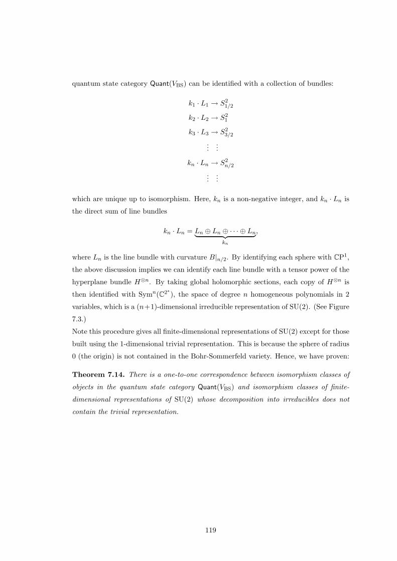
quantum state category Quant(VBS) can be identified with a collection of bundles:

k1 · L1 → S21/2

k2 · L2 → S21

k3 · L3 → S23/2

......

kn · Ln → S2n/2

......

which are unique up to isomorphism. Here, kn is a non-negative integer, and kn · Ln is

the direct sum of line bundles

kn · Ln = Ln ⊕ Ln ⊕ · · · ⊕ Ln︸ ︷︷ ︸kn

,

where Ln is the line bundle with curvature B|n/2. By identifying each sphere with CP1,

the above discussion implies we can identify each line bundle with a tensor power of the

hyperplane bundle H⊗n. By taking global holomorphic sections, each copy of H⊗n is

then identified with Symn(C2∗), the space of degree n homogeneous polynomials in 2

variables, which is a (n+1)-dimensional irreducible representation of SU(2). (See Figure

7.3.)

Note this procedure gives all finite-dimensional representations of SU(2) except for those

built using the 1-dimensional trivial representation. This is because the sphere of radius

0 (the origin) is not contained in the Bohr-Sommerfeld variety. Hence, we have proven:

Theorem 7.14. There is a one-to-one correspondence between isomorphism classes of

objects in the quantum state category Quant(VBS) and isomorphism classes of finite-

dimensional representations of SU(2) whose decomposition into irreducibles does not

contain the trivial representation.

119

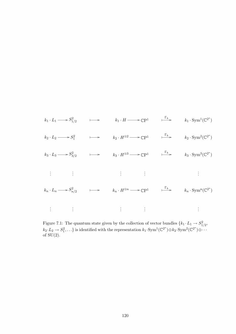
k1 · L1// S2

1/2 // k1 ·H // CP1 Γh // k1 · Sym1(C2∗)

k2 · L2// S2

1 // k2 ·H⊗2 // CP1 Γh // k2 · Sym2(C2∗)

k3 · L3// S2

3/2 // k3 ·H⊗3 // CP1 Γh // k3 · Sym3(C2∗)

......

......

...

kn · Ln // S2n/2

// kn ·H⊗n // CP1 Γh // kn · Symn(C2∗)

......

......

...

Figure 7.1: The quantum state given by the collection of vector bundles k1 ·L1 → S21/2,

k2 ·L2 → S21 , . . . is identified with the representation k1 ·Sym1(C2∗)⊕k2 ·Sym2(C2∗)⊕· · ·

of SU(2).

120

Chapter 8

Summary and future work

We conclude this thesis by providing a summary which ties together the main

results of the previous chapters. Along the way, we make some brief remarks regarding

open problems and possible directions for future research.

Polarizations on n-plectic manifolds

In Chapter 2, we presented the basic geometric facts needed for our study of

n-plectic manifolds. In particular, we considered the n-plectic analogues for Lagrangian

submanifolds and real polarizations. There are at least n different ways to generalize

the definition of a Lagrangian submanifold to n-plectic geometry. This is due to the

fact that there are n different ways to define the notion of orthogonal complement on

an n-plectic vector space (Def. 2.2). Since real polarizations in symplectic geometry are

foliations whose leaves are Lagrangian submanifolds, we have at least n different kinds of

real polarizations on an n-plectic manifold (Def. 2.13). Polarizations play an important

role in geometric quantization, but it is not clear which definition of polarization for

n-plectic manifolds is “best” in this context.

Moreover, it is unknown if an n-plectic analogue of a complex polarization

exists. It is possible that one could use ideas from generalized complex geometry [26]

and the theory of ‘higher Dirac structures’ [71] to help develop such polarizations.

Lie n-algebras from n-plectic manifolds

In Chapter 3, we showed that an n-plectic structure on M induces a bracket

on the space of Hamiltonian (n − 1)-forms. The bracket is skew-symmetric, but only

satisfies the Jacobi identity up to homotopy. We proved that this bracket gives a Lie

n-algebra L∞(M,ω), whose underlying n-term chain complex consists of Hamiltonian

121

(n− 1)-forms and all differential forms of lower degrees (Thm. 3.14). When n = 1, the

Hamiltonian forms are the smooth functions, and the Lie 1-algebra is just the underlying

Lie algebra of the usual Poisson algebra of a symplectic manifold. For certain 2-plectic

manifolds, our previous work with Baez and Hoffnung implies that the associated Lie

2-algebra can be used to describe the “observable algebra” of the classical bosonic string

[5].

In Appendix A, we showed that an n-plectic manifold also gives a dg Leibniz

algebra Leib(M,ω) on the same complex (Prop. A.3). Its bracket satisfies Jacobi, but

is skew-symmetric only up to homotopy. For the 2-plectic case, we showed L∞(M,ω)

and Leib(M,ω) are isomorphic in Roytenberg’s category of weak Lie 2-algebras (Thm.

A.10). The objects of this category are 2-term L∞-algebras whose structure maps are

skew-symmetric only up to homotopy. In general, we would like to conjecture that some

sort of equivalence such as this holds for n > 2. Unfortunately, it is not clear in what

category this should occur. Indeed, developing a theory of weak Lie n-algebras is an

open problem. Perhaps by studying the relationships between the structures specifically

on L∞(M,ω) and Leib(M,ω) for arbitrary n one could get a sense of what explicit

coherence conditions would be needed to give a good definition.

On the other hand, there are structures known as ‘Loday-∞ algebras’ (or sh

Leibniz algebras) [2] that generalize the definition of an L∞-algebra by, again, relaxing

the skew symmetry condition on the structure maps. However, this time the skew

symmetry is not required to hold up to homotopy. Hence any dg Leibniz algebra is a

Loday-∞ algebra. Any L∞-algebra is as well. Therefore there may be an isomorphism

between L∞(M,ω) and Leib(M,ω) in this category for n ≥ 2.

Lie 2-algebras from compact simple Lie groups

In Chapter 4, we considered compact simple Lie groups as 2-plectic manifolds.

Any compact simple Lie group G admits a 1 parameter family of canonical 2-plectic

structures νk, given by non-zero multiples of Cartan 3-form (Ex. 2.8). We proved

that the associated Lie 2-algebra L∞(G, νk) contains a sub Lie 2-algebra consisting of

left invariant Hamiltonian 1-forms (Cor. 4.4). We showed that this sub-algebra is not

equivalent to L∞(G, νk), however, it is isomorphic to the so-called string Lie 2-algebra

associated to (G, νk) (Thm. 4.7). The string Lie 2-algebra plays an important role in

string theory and in the theory of loop groups.

Our results suggest a close link between these areas and 2-plectic geometry.

There are many possible directions for future work here. In particular, it would be

122

interesting to understand the relationship between L∞(G, νk) and the algebra of observ-

ables for certain string theory models called ‘WZW models’.

Gerbes, 2-line stacks, and 2-bundles

In Chapter 5, we presented the technical tools needed to develop a geometric

quantization theory for 2-plectic manifolds. The work of Brylinski [13] implies that if

(M,ω) is a 2-plectic manifold and ω is an integral 3-form, then ω can be realized as the

2-curvature of a U(1)-gerbe equipped with a 2-connection. If Ui is an open cover of

M , then locally, a U(1)-gerbe with 2-connection is determined by a Deligne 2-cocycle

i.e a collection of U(1)-valued transition functions gijk on Ui ∩ Uj ∩ Uk, 1-forms Aij on

Ui ∩Uj , and 2-forms Bi on Ui, with dBi = ω, satisfying certain compatibility conditions

(Ex. 5.16).

Every principal U(1)-bundle with connection has an associated Hermitian line

bundle with connection. Similarly, we showed that every U(1)-gerbe with 2-connection

over a 2-plectic manifold has an associated 2-line stack with 2-connection (Prop. 5.32).

The category of global sections of the 2-line stack is equivalent to the category of Hermi-

tian vector bundles twisted by the gerbe’s Deligne 2-cocycle ξ = (gijk, Aij , Bi). Such a

twisted bundle is given locally by a collection of Hermitian vector bundles Ei with con-

nection ∇i (Def. 5.30). The twisting by ξ characterizes the obstruction to gluing these

bundles together into a global bundle over M . A ξ-twisted Hermitian vector bundle is

twisted-flat if, for each Ei, the curvature ∇2i is equal to

√−1 ·Bi ⊗ id (Def. 5.31). This

is the 2-plectic analogue of a flat section of a Hermitian line-bundle. We also showed

that there is a good notion of holonomy (Def. 5.36) for 2-line stacks equipped with 2-

connection, given by Carey, Johnson, and Murray’s formula for the 2-holonomy of the

Deligne class [ξ] [17]. The 2-holonomy plays an important role in our quantization pro-

cedure for 2-plectic manifolds. In particular, it is used in our definition for the 2-plectic

version of the Bohr-Sommerfeld variety (Def. 7.5).

It is not obvious, at first glance, why twisted Hermitian vector bundles are

the 2-plectic analogues of sections of a Hermitian line bundle. In the same chapter, we

sketch an argument supporting this point of view using Bartels’ work in 2-bundle theory

[10]. It becomes clear that twisted Hermitian vector bundles should be understood as

sections of a 2-vector bundle of rank 1. It would be very interesting to make this

argument more precise, and perhaps recast our results within the context of 2-vector

bundles. For example, for line bundles, one can consider different kinds of sections e.g.

smooth, square-integrable, etc. Similarly, the 2-bundle approach might suggest that

123

we consider 2-lines stacks whose sections are more general than twisted bundles, e.g.

twisted coherent sheaves. This could have important consequences for the output of our

geometric quantization procedure for 2-plectic manifolds.

2-Plectic prequantization and Courant algebroids

We defined a prequantized 2-plectic manifold to be a 2-plectic manifold equipped

with a Deligne 2-cocycle (Def. 6.2). This 2-cocycle can be realized geometrically as a

U(1)-gerbe with 2-connection, or as its associated 2-line stack. This is in complete anal-

ogy with the symplectic case, where we prequantize using either a principal U(1)-bundle

or a Hermitian line bundle. In Section 6.2 , we first recall how to prequantize the Poisson

algebra on a symplectic manifold equipped with a principal U(1)-bundle P with connec-

tion. By prequantizing, we mean faithfully representing the Poisson algebra as linear

differential operators. This is done by considering the Atiyah algebroid A associated

to P . There is an injective Lie algebra morphism from the Poisson algebra to the Lie

algebra of global sections of A, which identifies the Poisson algebra with those invariant

vector fields on P whose flows preserve the connection (Prop. 6.7).

For the 2-plectic case, we described a known construction which gives a Courant

algebroid C over a prequantized 2-plectic manifold (M,ω) equipped with a U(1)-gerbe

with 2-connection (Sec. 6.4). In this case, C is a vector bundle over M whose sections

are locally given by vector fields and 1-forms on M . Its space of global sections form a

Lie 2-algebra. There is a short exact sequence of vector bundles over M

T ∗M → C → TM,

whose splittings TM → C correspond to 2-connections on the U(1)-gerbe over M .

We prove the existence of an injective Lie 2-algebra morphism from the Lie 2-algebra

L∞(M,ω) of observables on M to the Lie 2-algebra L∞(C) of global sections of C

(Thm. 6.16). This morphism identifies L∞(M,ω) with a sub-Lie 2-algebra of L∞(C),

which, in a certain sense, preserves the 2-connection of the gerbe (Thm. 6.22). We

interpret this sub-algebra as the prequantization of L∞(M,ω). Also, we show that

this construction gives the higher analogue of the well known Kostant-Souriau central

extension in symplectic geometry (Sec. 6.5).

This prequantization process gives an interesting relationship between Courant

algebroids and prequantized 2-plectic manifolds. Let us give two possible directions for

future work based on these results.

1. Sections of the Atiyah algebroidA over a prequantized symplectic manifold equipped

with the principal U(1)-bundle are differential operators on a Hilbert space. This

124

Hilbert space is constructed from global sections of the associated Hermitian line

bundle. The higher analogue of this Hilbert space is the category of global sections

of the 2-line stack associated to a U(1)-gerbe. In what way, if at all, do sections of

the Courant algebroid over a prequantized 2-plectic manifold act as “operators”

on this higher analogue of a Hilbert space?

2. Recall that sections of the Atiyah algebroid are infinitesimal U(1)-equivariant sym-

metries of the corresponding principal U(1)-bundle. Integration gives the ‘gauge

groupoid’ over M , whose elements correspond to the equivariant automorphisms

of the principal bundle [15][Sec. 17.1]. Our results suggest that the Courant alge-

broid is the higher analogue of the Atiyah algebroid. So, how can we understand

sections of the Courant algebroid on a prequantized 2-plectic manifold as infinites-

imal automorphisms of the corresponding U(1)-gerbe? In other words, what is the

Lie 2-groupoid that integrates this Courant algebroid, and how does it act as the

‘gauge 2-groupoid’ of the U(1)-gerbe?

2-plectic quantization and representation theory

In the last chapter, we categorifed Sniatycki’s [62] quantization procedure for

symplectic manifolds, which employs Bohr-Sommerfeld varieties to overcome topological

obstructions that arise when using real polarizations (Sec. 7.2). This categorification

gives a simple procedure for quantizing a 2-plectic manifold, and the resulting output is a

category of quantum states (Def. 7.6). An object of this category is a twisted Hermitian

vector bundle over the Bohr-Sommerfeld variety (Def. 7.5) whose restriction to each leaf

contained in the variety is twisted-flat.

In Section 7.2.1, we considered an interesting example: M = R3 \0 equipped

with a volume form ω = dB. We quantized M by equipping it with the trivial Deligne

2-cocycle ξ = (1, 0, B), and a 2-polarization whose leaves are spheres centered about the

origin. The restriction of the 2-form B to such a sphere is the KKS symplectic form,

which arises in Kirillov’s orbit method for constructing representations of Lie groups.

This is not surprising, since R3 is isomorphic to the dual of the Lie algebra su(2), and

each sphere is isomorphic to a coadjoint orbit. We then showed that in this example, a

leaf of the polarization is contained in the Bohr-Sommerfeld variety if and only if it is

a sphere of radius n/2, where n is an integer (Cor. 7.12). The orbit method identifies

such a sphere with the irreducible representation of SU(2) whose dimension is n+ 1.

Next, we proved that any twisted bundle in the associated category of quantum

states is isomorphic to a direct sum of line bundles over spheres contained in the variety

125

(Thm. 7.13). The fact that the twisted bundle is twisted-flat on each sphere implies that

each of these line bundles must be isomorphic to a tensor power of the hyperplane bundle

over CP1. This allowed us to identify a quantum state with a representation of SU(2).

More precisely, we proved that isomorphism classes of objects in the quantum state

category are in one-to-one correspondence with isomorphism classes of finite-dimensional

representations of SU(2) whose decomposition into irreducibles does not contain the

trivial representation (Thm. 7.14).

It is unfortunate that we are unable to obtain the trivial representation via our

quantization procedure. However, it is not surprising. Our procedure identifies spheres

of radius n/2 with irreducibles of dimension n + 1. Hence, the trivial representation

corresponds to the origin in su(2)∗, which is not in M . In some sense, this identification

needs to be shifted so that the sphere of radius n/2 is identified with the irreducible

representation of dimension n. This is very similar to the 1/2 shift which arises in the

usual geometric quantization of the simple harmonic oscillator (Sec. 7.1.2).

We believe we have just scratched the surface of a deeper relationship between

representation theory and the geometric quantization of 2-plectic manifolds. Indeed,

our example suggests that 2-plectic quantization can give a categorifed analogue of the

orbit method. We conclude by mentioning two related directions for future work along

these lines.

1. It is well known that closed integral forms on a manifold M can be mapped

to closed integral forms on LM , the space of free loops of M , by a process

called ‘transgression’. Moreover, this process sends a U(1)-gerbe equipped with

2-connection on M to a principal U(1)-bundle with connection on LM [13][Ch. 6].

This suggests that the categorifed geometric quantization of a 2-plectic manifold

may, in some way, correspond to ordinary geometric quantization on LM . (We are

overlooking subtleties here, such as the fact that transgression need not preserve

non-degeneracy.) For example, perhaps there is some 2-plectic structure on su(2)

whose quantization gives a category of quantum states, with objects correspond-

ing to certain representations of the loop group LSU(2) obtained by applying the

orbit method to the loop algebra Lsu(2).

2. Much work has been done on quantizing the conjugacy classes of compact simple

Lie groups via a variety of methods, all of which rely on the Cartan 3-form in some

way [44, 46]. The output of these quantization procedures gives information about

the representation theory of the corresponding loop group. Every compact simple

Lie group, equipped with the Cartan 3-form, is a 2-plectic manifold. Hence, it is

126

natural to suspect that 2-plectic quantization of Lie groups is also related to the

representation theory of loop groups. We have preliminary results which suggest

that such a relationship exists, although, even in the simple case of SU(2), many

issues remain unresolved.

127

Bibliography

[1] W. Ambrose and I. M. Singer. A theorem on holonomy. Trans. Amer. Math. Soc.,75:428–443, 1953.

[2] M. Ammar and N. Poncin. Coalgebraic approach to the Loday infinity category,stem differential for 2n-ary graded and homotopy algebras. Ann. Inst. Fourier(Grenoble), 60(1):355–387, 2010. Also available as arXiv:0809.4328.

[3] B. Antieau. Cohomological obstruction theory for Brauer classes and the period-index problem. Available as arXiv:0909.2352.

[4] J. C. Baez and A. S. Crans. Higher-dimensional algebra. VI. Lie 2-algebras. TheoryAppl. Categ., 12:492–538, 2004. Also available as arXiv:math/0307263.

[5] J. C. Baez, A. E. Hoffnung, and C. L. Rogers. Categorified symplectic geometryand the classical string. Comm. Math. Phys., 293(3):701–725, 2010. Also availableas arXiv:0808.0246.

[6] J. C. Baez and C. L. Rogers. Categorified symplectic geometry and the string Lie2-algebra. Homology, Homotopy Appl., 12(1):221–236, 2010.

[7] J. C. Baez and U. Schreiber. Higher gauge theory. In Categories in Algebra,Geometry and Mathematical Physics, volume 431 of Contemp. Math., pages 7–30.Amer. Math. Soc., Providence, RI, 2007. Also available as arXiv:math/0511710.

[8] J. C. Baez, D. Stevenson, A. S. Crans, and U. Schreiber. From loop groupsto 2-groups. Homology, Homotopy Appl., 9(2):101–135, 2007. Also available asarXiv:math/0504123.

[9] G. Barnich, R. Fulp, T. Lada, and J. Stasheff. The sh Lie structure of Poissonbrackets in field theory. Comm. Math. Phys., 191(3):585–601, 1998. Also availableas arXiv:hep-th/9702176.

[10] T. Bartels. Higher Gauge Theory I: 2-Bundles. PhD thesis, University of California,Riverside, 2004. Available as arXiv:math/0410328.

[11] P. Bressler and A. Chervov. Courant algebroids. J. Math. Sci. (N. Y.), 128(4):3030–3053, 2005. Also available as arXiv:hep-th/0212195.

[12] J.-L. Brylinski. Noncommutative Ruelle-Sullivan type currents. In TheGrothendieck Festschrift, Vol. I, volume 86 of Progr. Math., pages 477–498.Birkhauser Boston, Boston, MA, 1990.

128

[13] J.-L. Brylinski. Loop Spaces, Characteristic Classes and Geometric Quantization.Modern Birkhauser Classics. Birkhauser Boston Inc., Boston, MA, 2008.

[14] A. Caldararu. Derived Categories of Twisted Sheaves on Calabi-Yau Manifolds.PhD thesis, Cornell University, 2000.

[15] A. Cannas da Silva and A. Weinstein. Geometric Models for Noncommutative Al-gebras, volume 10 of Berkeley Mathematics Lecture Notes. American MathematicalSociety, Providence, RI, 1999.

[16] F. Cantrijn, A. Ibort, and M. de Leon. On the geometry of multisymplectic mani-folds. J. Austral. Math. Soc. Ser. A, 66(3):303–330, 1999.

[17] A. L. Carey, S. Johnson, and M. K. Murray. Holonomy on D-branes. J. Geom.Phys., 52(2):186–216, 2004. Also available as arXiv:hep-th/0204199.

[18] T. J. Courant. Dirac manifolds. Trans. Amer. Math. Soc., 319(2):631–661, 1990.

[19] M. Forger, C. Paufler, and H. Romer. The Poisson bracket for Poisson forms inmultisymplectic field theory. Rev. Math. Phys., 15(7):705–743, 2003. Also availableas arXiv:math-ph/0202043.

[20] D. S. Freed. Higher algebraic structures and quantization. Comm. Math. Phys.,159(2):343–398, 1994. Also available as arXiv:hep-th/9212115.

[21] P. Gajer. Geometry of Deligne cohomology. Invent. Math., 127(1):155–207, 1997.Also available as arXiv:alg-geom/9601025.

[22] J. Giraud. Cohomologie non abelienne. Springer-Verlag, Berlin, 1971. DieGrundlehren der mathematischen Wissenschaften, Band 179.

[23] W. Greub, S. Halperin, and R. Vanstone. Connections, Curvature, and Cohomology.Vol. II: Lie Groups, Principal Bundles, and Characteristic Classes. Academic Press,New York-London, 1973.

[24] P. Griffiths and J. Harris. Principles of Algebraic Geometry. Wiley Classics Library.John Wiley & Sons Inc., New York, 1994.

[25] A. Grothendieck. Technique de descente et theoremes d’existence en geometriealgebrique. I. Generalites. Descente par morphismes fidelement plats. In SeminaireBourbaki, Vol. 5, pages Exp. No. 190, 299–327. Soc. Math. France, Paris, 1995.

[26] M. Gualtieri. Generalized complex geometry. Available as arXiv:math/0703298.

[27] F. Helein. Hamiltonian formalisms for multidimensional calculus of variations andperturbation theory. In Noncompact Problems at the Intersection of Geometry,Analysis, and Topology, volume 350 of Contemp. Math., pages 127–147. Amer.Math. Soc., Providence, RI, 2004. Also available as arXiv:math-ph/0212036.

[28] A. Henriques. Integrating L∞-algebras. Compos. Math., 144(4):1017–1045, 2008.Also available as arXiv:math/0603563.

[29] N. Hitchin. Generalized Calabi-Yau manifolds. Q. J. Math., 54(3):281–308, 2003.Also available as arXiv:math/0209099.

129

[30] A. Ibort. Multisymplectic geometry: generic and exceptional. In Proceedings of theIX Fall Workshop on Geometry and Physics (Vilanova i la Geltru, 2000), volume 3of Publ. R. Soc. Mat. Esp., pages 79–88. R. Soc. Mat. Esp., Madrid, 2001.

[31] M. M. Kapranov and V. A. Voevodsky. 2-categories and Zamolodchikov tetrahedraequations. In Algebraic Groups and Their Generalizations: Quantum and Infinite-dimensional Methods (University Park, PA, 1991), volume 56 of Proc. Sympos.Pure Math., pages 177–259. Amer. Math. Soc., Providence, RI, 1994.

[32] J. Kijowski. A finite-dimensional canonical formalism in the classical field theory.Comm. Math. Phys., 30:99–128, 1973.

[33] J. Kijowski and W. M. Tulczyjew. A Symplectic Framework for Field Theories,volume 107 of Lecture Notes in Physics. Springer-Verlag, Berlin, 1979.

[34] A. A. Kirillov. Lectures on the Orbit Method, volume 64 of Graduate Studies inMathematics. American Mathematical Society, Providence, RI, 2004.

[35] S. Kobayashi and K. Nomizu. Foundations of Differential Geometry. Vol I. JohnWiley & Sons, New York-London, 1963.

[36] Y. Kosmann-Schwarzbach. Derived brackets. Lett. Math. Phys., 69:61–87, 2004.Also available as arXiv:math/0312524.

[37] B. Kostant. Quantization and unitary representations. I. Prequantization. In Lec-tures in Modern Analysis and Applications, III, pages 87–208. Lecture Notes inMath., Vol. 170. Springer, Berlin, 1970.

[38] T. Lada and M. Markl. Strongly homotopy Lie algebras. Comm. Algebra,23(6):2147–2161, 1995. Also available as arXiv:hep-th/9406095.

[39] T. Lada and J. Stasheff. Introduction to SH Lie algebras for physicists. Internat.J. Theoret. Phys., 32(7):1087–1103, 1993. Also available as hep-th/9209099.

[40] Z.-J. Liu, A. Weinstein, and P. Xu. Manin triples for Lie bialgebroids. J. DifferentialGeom., 45(3):547–574, 1997. Also available as arXiv:dg-ga/9508013.

[41] K. C. H. Mackenzie. General Theory of Lie Groupoids and Lie Algebroids, volume213 of London Mathematical Society Lecture Note Series. Cambridge UniversityPress, Cambridge, 2005.

[42] J. Martinet. Sur les singularites des formes differentielles. Ann. Inst. Fourier(Grenoble), 20(fasc. 1):95–178, 1970.

[43] E. Meinrenken. The basic gerbe over a compact simple Lie group. Enseign. Math.(2), 49(3-4):307–333, 2003. Also available as arXiv:math/0209194.

[44] E. Meinrenken. On the quantization of conjugacy classes. Enseign. Math. (2),55(1-2):33–75, 2009. Also available as arXiv:0707.3963.

[45] I. Moerdijk. Introduction to the language of stacks and gerbes. Available asarXiv:math/0212266.

[46] S. Mohrdieck and R. Wendt. Integral conjugacy classes of compact Lie groups.Manuscripta Math., 113(4):531–547, 2004. Also available as arXiv:math/0303118.

130

[47] A. Pressley and G. Segal. Loop Groups. Oxford Mathematical Monographs. TheClarendon Press Oxford University Press, New York, 1986.

[48] D. Quillen. Rational homotopy theory. Ann. of Math. (2), 90:205–295, 1969.

[49] C. L. Rogers. 2-plectic geometry, Courant algebroids, and categorified prequanti-zation. Submitted. Available as arXiv:1009.2975.

[50] C. L. Rogers. L∞-algebras from multisymplectic geometry. To appear in Lett.Math. Phys. Available as arXiv:1005.2230.

[51] N. Roman-Roy. Multisymplectic Lagrangian and Hamiltonian formalisms of clas-sical field theories. SIGMA Symmetry Integrability Geom. Methods Appl., 5:Paper100, 25, 2009. Also available as arXiv:math-ph/0506022.

[52] D. Roytenberg. Courant Algebroids, Derived Brackets and Even Symplectic Su-permanifolds. PhD thesis, University of California, Berkeley, 1999. Available asarXiv:math/9910078.

[53] D. Roytenberg. On the structure of graded symplectic supermanifolds and Courantalgebroids. In Quantization, Poisson brackets and beyond (Manchester, 2001), vol-ume 315 of Contemp. Math., pages 169–185. Amer. Math. Soc., Providence, RI,2002. Also available as arXiv:math/0203110.

[54] D. Roytenberg. On weak Lie 2-algebras. In XXVI Workshop on Geometrical Meth-ods in Physics, volume 956 of AIP Conf. Proc., pages 180–198. Amer. Inst. Phys.,Melville, NY, 2007. Also available as arXiv:0712.3461.

[55] D. Roytenberg and A. Weinstein. Courant algebroids and strongly homo-topy Lie algebras. Lett. Math. Phys., 46(1):81–93, 1998. Also available asarXiv:math/9802118v1.

[56] H. Sati, U. Schreiber, and J. Stasheff. L∞-algebra connections and applications toString- and Chern-Simons n-transport. In Quantum Field Theory, pages 303–424.Birkhauser, Basel, 2009.

[57] P. Schapira. Categories, sites, sheaves and stacks: Course at University of Paris VI.Available as http://people.math.jussieu.fr/~schapira/lectnotes/Sta.pdf.

[58] M. Schlessinger and J. Stasheff. Deformation theory and rational homotopy type.1979. Preprint.

[59] U. Schreiber. ∞-Lie algebra cohomology. Available as http://ncatlab.org/nlab/show/infinity-Lie+algebra+cohomology.

[60] U. Schreiber. From Loop Space Mechanics to Nonabelian Strings. PhD thesis,Universitat Duisburg-Essen, 2005. Available as arXiv:hep-th/0509163.

[61] P. Severa and A. Weinstein. Poisson geometry with a 3-form background. Progr.Theoret. Phys. Suppl., (144):145–154, 2001. Also available as arXiv:math/0107133.

[62] J. Sniatycki. Wave functions relative to a real polarization. Internat. J. Theoret.Phys., 14(4):277–288, 1975.

131

[63] J. Sniatycki. Geometric Quantization and Quantum Mechanics, volume 30 of Ap-plied Mathematical Sciences. Springer-Verlag, New York, 1980.

[64] J.-M. Souriau. Quantification geometrique. Applications. Ann. Inst. H. PoincareSect. A (N.S.), 6:311–341, 1967.

[65] A. Swann. Hyper-Kahler and quaternionic Kahler geometry. Math. Ann.,289(3):421–450, 1991.

[66] P. Severa. Letter to Alan Weinstein. Available at http://sophia.dtp.fmph.uniba.sk/~severa/letters/.

[67] F. W. Warner. Foundations of Differentiable Manifolds and Lie Groups. Scott,Foresman and Co., Glenview, Ill.-London, 1971.

[68] H. Weyl. Geodesic fields in the calculus of variation for multiple integrals. Ann. ofMath. (2), 36(3):607–629, 1935.

[69] E. Witten. The index of the Dirac operator in loop space. In Elliptic Curvesand Modular Forms in Algebraic Topology (Princeton, NJ, 1986), volume 1326 ofLecture Notes in Math., pages 161–181. Springer, Berlin, 1988.

[70] N. Woodhouse. Geometric Quantization. The Clarendon Press Oxford UniversityPress, New York, 1980.

[71] M. Zambon. L∞-algebras and higher analogues of Dirac structures. Available asarXiv:1003.1004.

132

Appendix A

Other algebraic structures on

n-plectic manifolds

There are other structures besides Lie n-algebras which can generalize the

Poisson bracket to n-plectic manifolds. Here we show that any n-plectic manifold gives

rise to another kind of algebraic structure known as a differential graded (dg) Leibniz

algebra. A dg Leibniz algebra is a graded vector space equipped with a degree −1

differential and a bilinear bracket that satisfies a Jacobi-like identity, but does not need

to be skew-symmetric. There is an interesting relationship between the bilinear bracket

on the Lie n-algebra and the bracket on the corresponding dg Leibniz algebra. When

n = 2, these algebras can be compared directly as objects in Roytenberg’s category

of ‘weak Lie 2-algebras’ [54]. A weak Lie 2-algebra is a Lie 2-algebra whose k = 2

bracket satisfies skew-symmetry only up to a chain homotopy. This homotopy must

satisfy compatibility relations with the homotopy controlling the failure of the Jacobi

identity. We show that the Lie 2-algebra and the 2-term dg Leibniz algebra arising from

a 2-plectic manifold are isomorphic as weak Lie 2-algebras. We are unable to extend

this result to the n > 2 case, since there is currently no definition available for weak

L∞-algebras.

A.1 dg Leibniz algebras

In symplectic geometry, every function f ∈ C∞(M) is Hamiltonian. We also

have the equality:

f, g = ιvfdg = Lvf g (A.1)

133

for all f, g ∈ Ω0Ham (M) = C∞(M). Hence f, · is a degree zero derivation on Ω0

Ham (M),

which makes (Ω0Ham (M) , [·, ·]) a Poisson algebra. In general, for n > 1, an equality such

as Eq. A.1 does not hold, and Hamiltonian forms are obviously not closed under wedge

product. Therefore, we shouldn’t expect the Lie n-algebra L∞(M,ω) to behave like a

Poisson algebra. But we do have the following simple lemma:

Lemma A.1. Let (M,ω) be an n-plectic manifold. If α, β ∈ Ωn−1Ham (M) are Hamiltonian

forms, then

Lvαβ = α, β+ dιvαβ.

Proof. Definitions 3.1 and 3.3 imply:

Lvαβ = ιvαdβ + dιvαβ

= −ιvαιvβω + dιvαβ

= α, β+ dιvαβ.

Lemma A.1 suggests that we interpret the (n − 1)-form Lvαβ as a type of

bracket on Ωn−1Ham (M), equal to the bracket ·, · modulo boundary terms. To this end,

we consider an algebraic structure known as a differential graded (dg) Leibniz algebra.

Definition A.2. A differential graded Leibniz algebra (L, δ, J·, ·K) is a graded vector

space L equipped with a degree -1 linear map δ : L → L and a degree 0 bilinear map

J·, ·K : L⊗ L→ L such that the following identities hold:

δ δ = 0 (A.2)

δ Jx, yK = Jδx, yK + (−1)|x| Jx, δyK (A.3)

Jx, Jy, zKK = JJx, yK , zK + (−1)|x||y| Jy, Jx, zKK , (A.4)

for all x, y, z ∈ L.

In the literature, dg Leibniz algebras are also called dg Loday algebras. This

definition presented here is equivalent to the one given by Ammar and Poncin [2]. Note

that the second condition given in the definition above can be interpreted as the Jacobi

identity. Hence if the bilinear map J·, ·K is skew-symmetric, then a dg Leibniz algebra is

a DGLA.

We now show that every n-plectic manifold gives a dg Leibniz algebra.

134

Proposition A.3. Given an n-plectic manifold (M,ω), there is a differential graded

Leibniz algebra Leib(M,ω) = (L, δ, J·, ·K) with underlying graded vector space

Li =

Ωn−1Ham (M) i = 0,

Ωn−1−i(M) 0 < i ≤ n− 1,

and maps δ : L→ L, J·, ·K : L⊗ L→ L defined as

δ(α) = dα,

if |α| > 0 and

Jα, βK =

Lvαβ if |α| = 0,

0 if |α| > 0,

where vα is the Hamiltonian vector field associated to α.

Proof. If α, β ∈ L0 = Ωn−1Ham (M) are Hamiltonian, then Lemma A.1 implies d Jα, βK =

d α, β = −ι[vα,vβ ]ω. Hence Jα, βK is Hamiltonian. For |β| > 0, we have |Lvαβ| = |β|,since the Lie derivative is a degree zero derivation. Hence J·, ·K is a bilinear degree 0

map.

We next show that Eq. A.3 of Definition A.2 holds. If |α| > 1, then it holds

trivially. If |α| = 1, then Jα, βK = Jα, δβK = 0 for all β ∈ L by definition, and Jδα, βK = 0

since the Hamiltonian vector field associated to dα is zero. If |α| = 0 and |β| = 0, then

|Jα, βK| = 0. Hence all terms in (A.3) vanish by definition. The last case to consider is

|α| = 0 and |β| > 0. We have

δ Jα, βK = dLvαβ = Lvαdβ = Jα, δβK .

Finally, we show the Jacobi identity (A.4) holds. Let α, β, γ ∈ L. Then

the left hand side of (A.4) is Jα, Jβ, γKK, while the right hand side is JJα, βK , γK +

(−1)|α||β| Jβ, Jα, γKK. Note equality holds trivially if |α| > 0 or |β| > 0. Otherwise,

we use the identity

L[v1,v2] = Lv1Lv2 − Lv2Lv1 ,

and the fact that d Jα, βK = −ι[vα,vβ ]ω to obtain the following equalities:

Jα, Jβ, γKK = LvαLvβγ

= L[vα,vβ ]γ + LvβLvαγ

= JJα, βK , γK + Jβ, Jα, γKK .

135

One interesting aspect of the dg Leibniz structure is that it interprets the

bracket of Hamiltonian (n−1)-forms geometrically as the change of an observable along

the flow of a Hamiltonian vector field. Leibniz algebras, in fact, naturally arise in a

variety of geometric settings e.g. in Courant algebroid theory and, more generally, in

the derived bracket formalism [36]. It would be interesting to compare Leib(M,ω) to

the Leibniz algebras that appear in these other formalisms.

A.2 Weak Lie 2-algebras

When (M,ω) is a symplectic manifold, L∞(M,ω) and Leib(M,ω) give the same

Lie algebra: the Poisson algebra of functions. It would be nice if we could show that for

any n-plectic manifold, L∞(M,ω) and Leib(M,ω) are also “the same”, i.e. equivalent

as objects in some category containing both L∞-algebras and dg Leibniz algebras. This

may seem unlikely at first since the brackets which induce these structures have different

properties. For example, ·, · is skew-symmetric, while J·, ·K, in general, is not. However,

we have the following proposition.

Proposition A.4. Let (M,ω) be an n-plectic manifold, and ·, · and J·, ·K be the brack-

ets given in Def. 3.3 and Prop. A.3, respectively. If α and β are Hamiltonian (n − 1)-

forms, then

Jα, βK + Jβ, αK = d(ιvαβ + ιvβα

).

Proof. The statement follows from the formula Lv = ιvd+ dιv.

So, we seek a category whose objects originate from weakening, up to homo-

topy, both the skew-symmetric axiom and the Jacobi identity. Unfortunately, no such

category exists, unless n = 2. In this case, by extending the work of Baez and Crans

[4], Roytenberg [54] developed what are known as 2-term weak L∞-algebras, or ‘weak

Lie 2-algebras’. In a weak Lie 2-algebra, the skew symmetry condition on the maps

given in Definition 3.7 is relaxed. In particular, the bilinear map l2 : L⊗L→ L is skew-

symmetric only up to homotopy. This homotopy must satisfy a coherence condition,

as well as compatibility conditions with the homotopy that controls the failure of the

Jacobi identity. The goal of this section is to show that if (M,ω) is a 2-plectic manifold,

then L∞(M,ω) and Leib(M,ω) are isomorphic as weak Lie 2-algebras.

Definition A.5 ([54]). A weak Lie 2-algebra is a 2-term chain complex of vector

spaces L = (L1d→ L0) equipped with the following structure:

• a chain map [·, ·] : L⊗ L→ L called the bracket;

136

• a chain homotopy S : L⊗ L→ L from the chain map

L⊗ L → L

x⊗ y 7−→ [x, y]

to the chain mapL⊗ L → L

x⊗ y 7−→ −[y, x]

called the alternator;

• a chain homotopy J : L⊗ L⊗ L→ L from the chain map

L⊗ L⊗ L → L

x⊗ y ⊗ z 7−→ [x, [y, z]]

to the chain map

L⊗ L⊗ L → L

x⊗ y ⊗ z 7−→ [[x, y], z] + [y, [x, z]]

called the Jacobiator.

In addition, the following equations are required to hold:

[x, J(y, z, w)] + J(x, [y, z], w) + J(x, z, [y, w]) + [J(x, y, z), w]

+[z, J(x, y, w)] = J(x, y, [z, w]) + J([x, y], z, w)

+[y, J(x, z, w)] + J(y, [x, z], w) + J(y, z, [x,w]),

(A.5)

J(x, y, z) + J(y, x, z) = −[S(x, y), z], (A.6)

J(x, y, z) + J(x, z, y) = [x, S(y, z)]− S([x, y], z)− S(y, [x, z]), (A.7)

S(x, [y, z]) = S([y, z], x). (A.8)

A weak Lie 2-algebra homomorphism is a chain map between the underly-

ing chain complexes that preserves the bracket up to coherent chain homotopy. More

precisely:

Definition A.6 ([54]). Given Lie 2-algebras L and L′ with bracket, alternator and

Jacobiator [·, ·], S, J and [·, ·]′, S′, J ′ respectively, a homomorphism from L to L′

consists of:

• a chain map φ = (φ0, φ1) : L→ L′, and

137

• a chain homotopy Φ: L⊗ L→ L′ from the chain map

L⊗ L → L′

x⊗ y 7−→ [φ(x), φ(y)]′ ,

to the chain mapL⊗ L → L′

x⊗ y 7−→ φ ([x, y])

such that the following equations hold:

S′ (φ0(x), φ0(y))− φ1(S (x, y)) = Φ(x, y) + Φ(y, x), (A.9)

J ′ (φ0(x), φ0(y), φ0(z))− φ1 (J (x, y, z))

= [φ0(x),Φ(y, z)]′ − [φ0(y),Φ(x, z)]′ − [Φ(x, y), φ0(z)]′

−Φ([x, y], z)− Φ(y, [x, z]) + Φ(x, [y, z]).

(A.10)

The details involved in composing Lie 2-algebra homomorphisms are given by Royten-

berg [54]. We say a Lie 2-algebra homomorphism with an inverse is an isomorphism.

Lie 2-algebras in the sense of Prop. 3.10 are weak Lie 2-algebras that satisfy

skew-symmetry on the nose. They are called semi-strict Lie 2-algebras in this context,

since the Jacobi identity may still fail to hold. More precisely:

Definition A.7 ([54]). A weak Lie 2-algebra (L, [·, ·], S, J) is semi-strict iff S = 0,

and hemi-strict iff J = 0.

Note that the bracket of a hemi-strict Lie 2-algebra satisfies a Jacobi identity

of the form

[x, [y, z]]− [[x, y], z]− [y, [x, z]] = 0,

but it is not necessarily skew-symmetric. In fact, any hemi-strict Lie 2-algebra is a

2-term dg Leibniz algebra. For 2-plectic manifolds, we have a converse:

Proposition A.8. If (M,ω) is a 2-plectic manifold, then Leib(M,ω) is a hemi-strict

Lie 2-algebra with:

• underlying complex

L = C∞(M) d→ Ω1Ham (M) ,

• bracket given by

[α, β] = Jα, βK = Lvαβ,

138

in degree 0, and

[α, f ] = Jα, fK = Lvαf,

[f, α] = Jf, αK = 0

in degree 1,

• alternator given by:

S(α, β) = ιvαβ + ιvβα,

• Jacobiator given by:

J(α, β, γ) = 0.

Proof. The axioms for a weak Lie 2-algebra given in Def. A.5 are verified by straight-

forward calculations using the Cartan calculus. In particular, the fact that Eq. A.7 is

satisfied follows from the identity:

Lvιwα = ι[v,w]α+ ιwLvα.

For a 2-plectic manifold, we view L∞(M,ω) as a weak Lie 2-algebra with trivial

alternator.

Proposition A.9. If (M,ω) is a 2-plectic manifold, then L∞(M,ω) is a semi-strict Lie

2-algebra with:

• underlying complex

L = C∞(M) d→ Ω1Ham (M) ,

• bracket given by

[α, β] = α, β = ω(vα, vβ, ·),

in degree 0, and

[α, f ] = 0

[f, α] = 0

in degree 1,

• alternator given by:

S(α, β) = 0,

139

• Jacobiator given by:

J(α, β, γ) = ω(vγ , vβ, vα).

Proof. By setting S = 0, in Def. A.5, we recover the usual notion of a Lie 2-algebra Def.

3.8. Hence, the statement follows from Prop. 3.15.

The main result of this section is the following theorem:

Theorem A.10. If (M,ω) is a 2-plectic manifold, then L∞(M,ω) and Leib(M,ω) are

isomorphic as weak Lie 2-algebras.

Proof. Since the underlying chain complexes of L∞(M,ω) and Leib(M,ω) are the same,

we build a weak Lie 2-algebra isomorphism (Def. A.6) using the identity chain map

φ0 = id, φ1 = id .

Let Φ: Ω1Ham (M)⊗ Ω1

Ham (M)→ C∞(M) be the map:

Φ(α, β) = ιvαβ.

Proposition A.4 and a straightforward calculation show that Φ gives a chain homotopy:

L0 ⊗ L1 ⊕ L1 ⊗ L0

[·,·]−[·,·]′

// L0 ⊗ L0

Φ

tti i i i i i i i i i

[·,·]−[·,·]′

L′1d // L′0

where L1 = L′1 = C∞(M), L0 = L′0 = Ω1Ham (M), [·, ·] is the bracket on Leib(M,ω), and

[·, ·]′ is the bracket on L∞(M,ω).

The alternator for Leib(M,ω) is

S(α, β) = ιvαβ + ιvβα = Φ(α, β) + Φ(β, α).

Since the alternator for L∞(M,ω) is trivial, the above equality implies Eq. A.9 in Def.

A.6 holds.

Since the Jacobiator of Leib(M,ω) is trivial, the left hand side of Eq. A.10 only

involves the Jacobiator J ′(α, β, γ) = ω(vγ , vβ, vα) of L∞(M,ω). Using the definition of

the brackets [·, ·] and [·, ·]′, the right hand side of Eq. A.10 becomes:

Jα,Φ(β, γ)K− Jβ,Φ(α, γ)K− JΦ(α, β), γK − Φ(α, β , γ)− Φ(β, α, γ) + Φ(α, β, γ).

By expanding the above using Φ(α, β) = ιvαβ, JΦ(α, β), γK = 0, Jα,Φ(β, γ)K = LvαΦ(β, γ),

Jα, βK = ω(vα, vβ, ·), and the identity

Lvιwα = ι[v,w]α+ ιwLvα,

140

the right hand side of Eq. A.10 becomes:

ιvβdιvαγ + ιvβ ιvαdγ − ιvβdιvαγ + 2ω(vα, vβ, vγ).

Since ω(vα, vβ, vγ) = −ιvβ ιvαdγ, the above expression simplifies to:

ω(vα, vβ, vγ) = −ω(vγ , vβ, vα) = −J ′(α, β, γ),

which is the left hand side of Eq. A.10. Hence, (φ0, φ1,Φ) satisfies the axioms for an

isomorphism of weak Lie 2-algebras.

141

Appendix B

Twisted bundles and the proof of

Proposition 5.28

Recall Def. 5.25 of a Hermitian vector bundle twisted by a 2-cocycle g ∈C2(U ,U(1)) on an open cover U = Ui of a manifold M . Such an object is given

by the following data:

• on each Ui, a Hermitian vector bundle

(Ei, 〈·, ·〉i),

• on each Uij = Ui ∩ Uj , an isomorphism of Hermitian vector bundles

φij : Ej |Uij∼→ Ei|Uij ,

such that ∀i, j, k ∈ I:

φ−1ik φij φjk = gijk·

where gijk· is the automorphism of Ek|Uijk corresponding to multiplication by

gijk : Ui ∩ Uj ∩ Uk → U(1).

Also, recall that a morphism f : (Ei, φij) → (E′i, φ′ij) of g-twisted Hermitian vector

bundles over M consists of a collection of morphisms of Hermitian vector bundles

fi : Ei → E′i,

for each i ∈ I such that

fi φij = φ′ij fj .

In this section, we will prove Prop. 5.28 from Chapter 5:

142

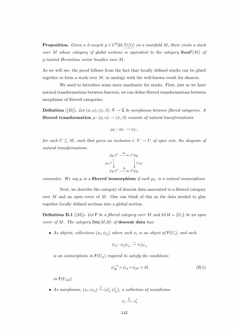
Proposition. Given a 2-cocycle g ∈ C2(U ,U(1)) on a manifold M , there exists a stack

over M whose category of global sections is equivalent to the category Bundg(M) of

g-twisted Hermitian vector bundles over M .

As we will see, the proof follows from the fact that locally defined stacks can be glued

together to form a stack over M , in analogy with the well-known result for sheaves.

We need to introduce some more machinery for stacks. First, just as we have

natural transformations between functors, we can define fibered transformations between

morphisms of fibered categories:

Definition ([45]). Let (φ, α), (ψ, β) : F→ G be morphisms between fibered categories. A

fibered transformation µ : (φ, α)→ (ψ, β) consists of natural transformations

µU : φU → ψU ,

for each U ⊆ M , such that given an inclusion i : V → U of open sets, the diagram of

natural transformations

φV i∗

µV i∗

αi // i∗φU

i∗µU

ψV i∗ βi // i∗ψU

commutes. We say µ is a fibered isomorphism if each µU is a natural isomorphism.

Next, we describe the category of descent data associated to a fibered category

over M and an open cover of M . One can think of this as the data needed to glue

together locally defined sections into a global section.

Definition B.1 ([45]). Let F be a fibered category over M and let U = Ui be an open

cover of M . The category Des(M,U) of descent data has:

• As objects, collections (xi, ψij) where each xi is an object of F(Ui), and each

ψij : xj |Uij∼→ xi|Uij

is an isomorphism in F(Uij) required to satisfy the conditions

ψ−1ik ψij ψjk = id (B.1)

in F(Uijk).

• As morphisms, (xi, ψij)f−→ (x′i, ψ

′ij), a collection of morphisms

xifi−→ x′i

143

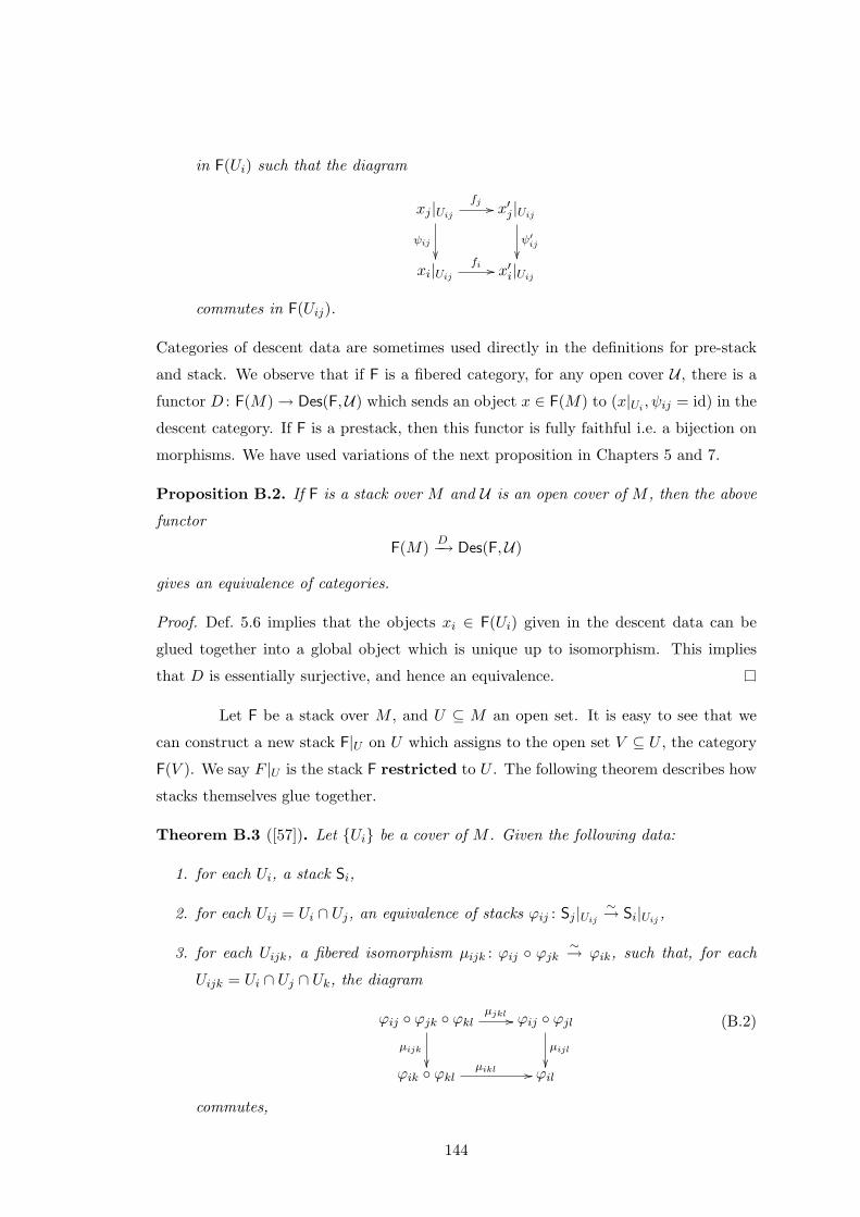
in F(Ui) such that the diagram

xj |Uijψij

fj // x′j |Uijψ′ij

xi|Uij

fi // x′i|Uij

commutes in F(Uij).

Categories of descent data are sometimes used directly in the definitions for pre-stack

and stack. We observe that if F is a fibered category, for any open cover U , there is a

functor D : F(M)→ Des(F,U) which sends an object x ∈ F(M) to (x|Ui , ψij = id) in the

descent category. If F is a prestack, then this functor is fully faithful i.e. a bijection on

morphisms. We have used variations of the next proposition in Chapters 5 and 7.

Proposition B.2. If F is a stack over M and U is an open cover of M , then the above

functor

F(M) D−→ Des(F,U)

gives an equivalence of categories.

Proof. Def. 5.6 implies that the objects xi ∈ F(Ui) given in the descent data can be

glued together into a global object which is unique up to isomorphism. This implies

that D is essentially surjective, and hence an equivalence.

Let F be a stack over M , and U ⊆ M an open set. It is easy to see that we

can construct a new stack F|U on U which assigns to the open set V ⊆ U , the category

F(V ). We say F |U is the stack F restricted to U . The following theorem describes how

stacks themselves glue together.

Theorem B.3 ([57]). Let Ui be a cover of M . Given the following data:

1. for each Ui, a stack Si,

2. for each Uij = Ui ∩ Uj, an equivalence of stacks ϕij : Sj |Uij∼→ Si|Uij ,

3. for each Uijk, a fibered isomorphism µijk : ϕij ϕjk∼→ ϕik, such that, for each

Uijk = Ui ∩ Uj ∩ Uk, the diagram

ϕij ϕjk ϕklµijk

µjkl // ϕij ϕjlµijl

ϕik ϕkl

µikl // ϕil

(B.2)

commutes,

144

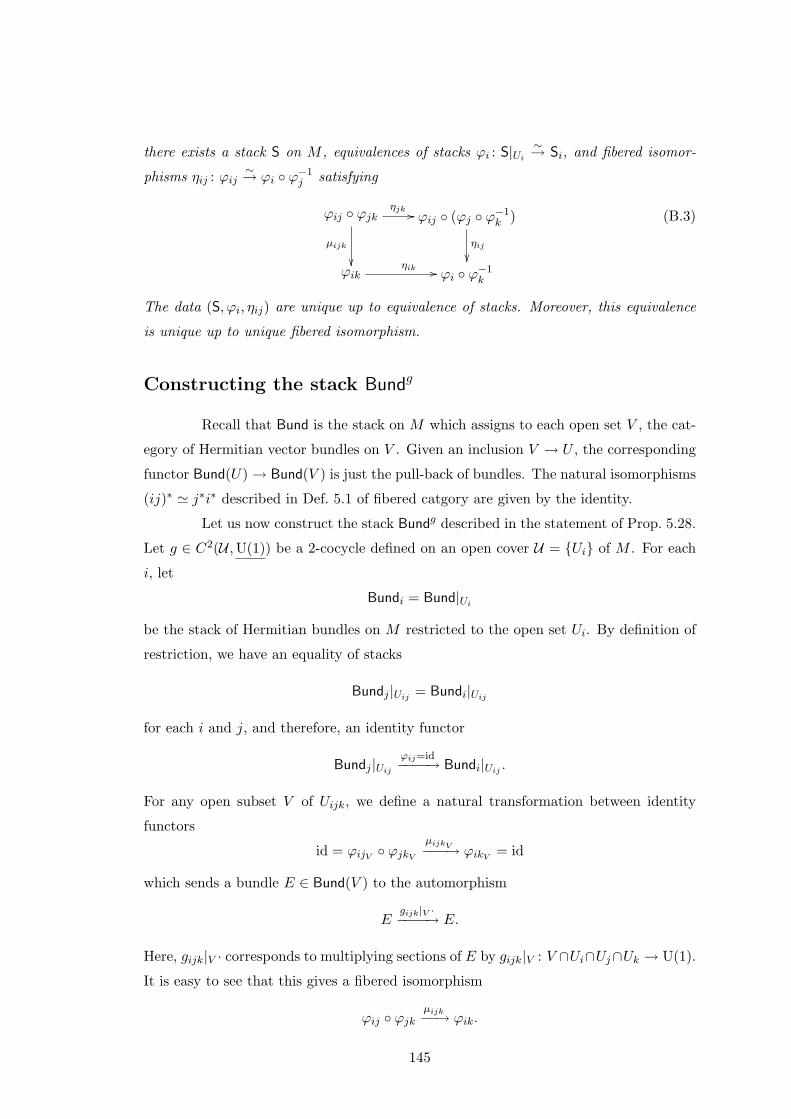
there exists a stack S on M , equivalences of stacks ϕi : S|Ui∼→ Si, and fibered isomor-

phisms ηij : ϕij∼→ ϕi ϕ−1

j satisfying

ϕij ϕjk

µijk

ηjk // ϕij (ϕj ϕ−1k )

ηij

ϕik

ηik // ϕi ϕ−1k

(B.3)

The data (S, ϕi, ηij) are unique up to equivalence of stacks. Moreover, this equivalence

is unique up to unique fibered isomorphism.

Constructing the stack Bundg

Recall that Bund is the stack on M which assigns to each open set V , the cat-

egory of Hermitian vector bundles on V . Given an inclusion V → U , the corresponding

functor Bund(U)→ Bund(V ) is just the pull-back of bundles. The natural isomorphisms

(ij)∗ ' j∗i∗ described in Def. 5.1 of fibered catgory are given by the identity.

Let us now construct the stack Bundg described in the statement of Prop. 5.28.

Let g ∈ C2(U ,U(1)) be a 2-cocycle defined on an open cover U = Ui of M . For each

i, let

Bundi = Bund|Ui

be the stack of Hermitian bundles on M restricted to the open set Ui. By definition of

restriction, we have an equality of stacks

Bundj |Uij = Bundi|Uij

for each i and j, and therefore, an identity functor

Bundj |Uijϕij=id−−−−→ Bundi|Uij .

For any open subset V of Uijk, we define a natural transformation between identity

functors

id = ϕijV ϕjkVµijkV−−−→ ϕikV = id

which sends a bundle E ∈ Bund(V ) to the automorphism

Egijk|V ·−−−−→ E.

Here, gijk|V · corresponds to multiplying sections of E by gijk|V : V ∩Ui∩Uj∩Uk → U(1).

It is easy to see that this gives a fibered isomorphism

ϕij ϕjkµijk−−→ ϕik.

145

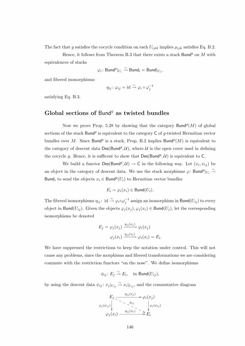
The fact that g satisfies the cocycle condition on each Uijkl implies µijk satisfies Eq. B.2.

Hence, it follows from Theorem B.3 that there exists a stack Bundg on M with

equivalences of stacks

ϕi : Bundg|Ui∼→ Bundi = Bund|Ui ,

and fibered isomorphisms

ηij : ϕij = id ∼→ ϕi ϕ−1j

satisfying Eq. B.3.

Global sections of Bundg as twisted bundles

Now we prove Prop. 5.28 by showing that the category Bundg(M) of global

sections of the stack Bundg is equivalent to the category C of g-twisted Hermitian vector

bundles over M . Since Bundg is a stack, Prop. B.2 implies Bundg(M) is equivalent to

the category of descent data Des(Bundg,U), where U is the open cover used in defining

the cocycle g. Hence, it is sufficent to show that Des(Bundg,U) is equivalent to C.

We build a functor Des(Bundg,U) → C in the following way. Let (xi, ψij) be

an object in the category of descent data. We use the stack morphisms ϕ : Bundg|Ui∼→

Bundi to send the objects xi ∈ Bundg(Ui) to Hermitian vector bundles

Ei = ϕi(xi) ∈ Bund(Ui).

The fibered isomorphisms ηij : id ∼→ ϕiϕ−1j assign an isomorphism in Bund(Uij) to every

object in Bund(Uij). Given the objects ϕj(xj), ϕj(xi) ∈ Bund(Uj), let the corresponding

isomorphisms be denoted

Ej = ϕj(xj)ηij(xj)−−−−→ ϕi(xj)

ϕj(xi)ηij(xi)−−−−→ ϕi(xi) = Ei.

We have suppressed the restrictions to keep the notation under control. This will not

cause any problems, since the morphisms and fibered transformations we are considering

commute with the restriction functors “on the nose”. We define isomorphisms

φij : Ej∼→ Ei, in Bund(Uij),

by using the descent data ψij : xj |Uij∼→ xi|Uij , and the commutative diagram

Ej

ϕj(ψij)

φij

((PPPPPPPPηij(xj) // ϕi(xj)

ϕi(ψij)

ϕj(xi)

ηij(xi) // Ei

146

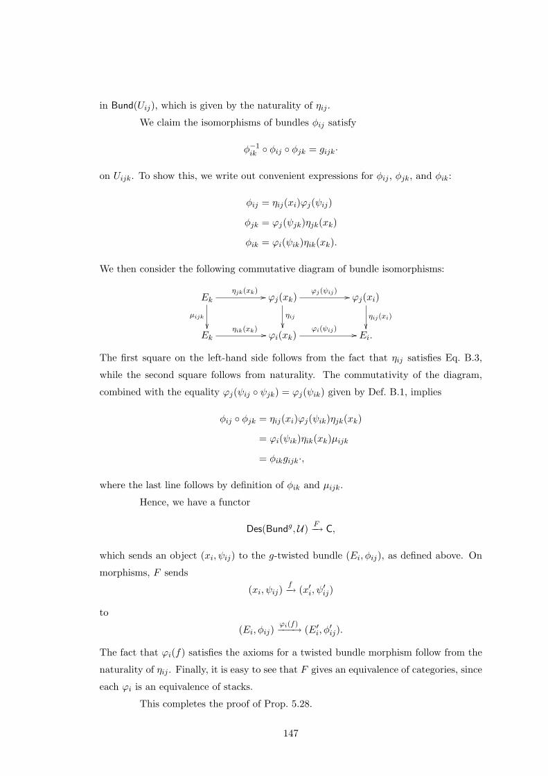
in Bund(Uij), which is given by the naturality of ηij .

We claim the isomorphisms of bundles φij satisfy

φ−1ik φij φjk = gijk·

on Uijk. To show this, we write out convenient expressions for φij , φjk, and φik:

φij = ηij(xi)ϕj(ψij)

φjk = ϕj(ψjk)ηjk(xk)

φik = ϕi(ψik)ηik(xk).

We then consider the following commutative diagram of bundle isomorphisms:

Ek

µijk

ηjk(xk)// ϕj(xk)

ηij

ϕj(ψij) // ϕj(xi)

ηij(xi)

Ek

ηik(xk) // ϕi(xk)ϕi(ψij) // Ei.

The first square on the left-hand side follows from the fact that ηij satisfies Eq. B.3,

while the second square follows from naturality. The commutativity of the diagram,

combined with the equality ϕj(ψij ψjk) = ϕj(ψik) given by Def. B.1, implies

φij φjk = ηij(xi)ϕj(ψik)ηjk(xk)

= ϕi(ψik)ηik(xk)µijk

= φikgijk·,

where the last line follows by definition of φik and µijk.

Hence, we have a functor

Des(Bundg,U) F−→ C,

which sends an object (xi, ψij) to the g-twisted bundle (Ei, φij), as defined above. On

morphisms, F sends

(xi, ψij)f−→ (x′i, ψ

′ij)

to

(Ei, φij)ϕi(f)−−−→ (E′i, φ

′ij).

The fact that ϕi(f) satisfies the axioms for a twisted bundle morphism follow from the

naturality of ηij . Finally, it is easy to see that F gives an equivalence of categories, since

each ϕi is an equivalence of stacks.

This completes the proof of Prop. 5.28.

147