Highly Preliminary Draft

Life Cycle Earnings and Saving in a Fast-Growing Economy�

Zheng Michael SongFudan University and Chinese University of Hong Kong

Dennis Tao YangChinese University of Hong Kong

June 21, 2010

Abstract

Rising saving rate� particularly among young households� in rapidly grow-ing economies presents a puzzle because forward-looking consumers shouldsave less when they anticipate future income growth. This paper proposes aresolution of the puzzle by documenting dramatic �attening of age-earningpro�les during a period of extraordinary growth in China. We show thatonce this structural shift in earnings is incorporated, an otherwise standardintertemporal choice model can explain the observed saving behavior. Ourquantitative analysis based on dynamic optimization of heterogeneous agentsaccounts well for the recent surge in household saving as well as the U-shapedincrease in saving rates over the life cycle in China.

Keywords: Household saving, age-earning pro�le, income growth, intertem-poral choice, life-cycle model, China.

JEL classi�cation: E21, D91, O53

�We would like to thank Jing Han, Kjetil Storesletten, Hongliang Zhang, Xiaodong Zhu, and seminar par-ticipants at The Chinese University of Hong Kong, Shanghai Jiaotong University, University of Hong Kong,Tsinghua Macro Workshop on Saving and Investment and the First Annual International Conference on theChinese Economy at HKIMR for helpful comments. The remaining erros are our own. Contact information:Song, Department of Economics, The Chinese University of Hong Kong, E-mail: zsong@fudan.edu.cn; Yang,Department of Economics, The Chinese University of Hong Kong, E-mail: deyang@cuhk.edu.hk.

1 Introduction

Households save more in fast-growing economies. The respective experiences of the East Asian

countries, such as Japan in the 1970s and Korea and Taiwan in the 1980s, attest to this

empirical regularity. In the last decade, rising saving in the BRIC countries provides further

evidence.1 However, these observations are di¢ cult to reconcile with the representative agent

model, since forward-looking consumers with standard preference should save less in a high-

growth environment as they anticipate a higher level of earnings in the future relative to their

present incomes (e.g., Tobin, 1967; Carroll and Summers, 1991). Although income growth can

lead to increased saving in the life-cycle model (e.g., Modigliani, 1970) or in models with habit

formation (e.g., Carroll, Overland and Weil, 2000), the quantitative e¤ect has shown to be

small (e.g., Paxson, 1996). This is the household saving puzzle that remains unresolved .

Behind the rise in average saving, there is a second stylized fact regarding life-cycle saving

pro�les. When Taiwan experienced rapid income growth in the period 1976-1990, the saving

rates of young households were systematically higher than that of the old households (Deaton

and Paxson, 1994). This empirical regularity is also observed in China. From 1992 to 2007,

the average saving rate of young households with their heads under age 40 increased by about

11 percentage points (see Figure 3B).2 The high saving of the young in these two fast-growing

economies contrasts sharply with the typical hump-shaped or relatively �at age-saving pro-

�les in developed economies. If growth raises the earnings of all workers, why don�t young

households consume more with higher future income?

The goal of this paper is to show that the high-saving puzzle in fast-growing economies

can be resolved in a model of intertemporal choice, once we allow for structural shifts in life-

cycle earning pro�les associated with high economic growth. Using unique and comprehensive

Urban Household Survey data (UHS) covering the period 1992-2007, we document two striking

changes in individual age-earning pro�les in the fast-growing economy of China: (a) there

were large upward shifts in the earnings of successive younger worker cohorts, and (b) the

age-earning pro�les have become �attened during this period. These empirical �ndings are1Between 1998 and 2008, the real annual GDP growth of Brazil, China, India and Russia are 3.3%, 9.8%,

7.2% and 6.9%, respectively. During the same period, the increase in their gross domestic saving as percentageof GDP are 4.1%, 7.8%, 11.9% and 14.6%, reaching an average saving rate of 34.4% for the BRIC countries,exceeding the world average by 12 percentage points in 2008 (Yang, Zhang and Zhou, 2010).

2These �ndings are based on the national sample of China�s Urban Household Surveys (UHS), which isdescribed in details in the Data Appendix. Chamon and Prasad (2010) is the �rst to document high savingrates for young households in urban China, which is con�rmed by Yang, Zhang and Zhou (2010), both usingthe UHS data for selected provinces and time periods.

1

at variance with a stable age-earning pro�le, an assumption made in virtually all models of

life-cycle saving decisions.

To illuminate how observed changes in earning pro�les a¤ect saving decisions through a

transparent mechanism, we develop a simple four-period overlapping generation (OLG) model

with closed-form solutions. We �nd that when the economy begins high income growth, workers

of all ages choose a higher rate of saving; and, with the �attening of age-earning pro�les, young

workers raise their saving rate more pronounced than older workers. These results are robust

to incorporating within-generation heterogeneity in worker types, the inclusion of a pension

system, and alternative speci�cations of perfect-foresight and myopic expectations of lifetime

earnings. These results provide a novel mechanism for explaining the rise in saving rate�

particularly among young households� in fast-growing economies.

The remaining question is quantitative: To what extent can the observed �attening earning

pro�les with income growth explain the increase in aggregate saving, the rise in the saving

rate of the young, and other saving behavior over the life cycle in China? Between 1992

and 2007, China�s GDP per capita grew at a remarkable annual rate of 8.5 percent, while

the aggregate urban household saving rate increased from 16.6 to 27.6 percent. In addition,

consistent with Chamon and Prasad (2010), our national sample of UHS data also show that

the age pro�les of saving in China exhibit a U-shaped pattern in recent years, with younger

and older households having relatively high saving rates (see Figure 3A). There is a more

pronounced U-shaped increase in age-speci�c saving rates across the initial (1992-1993) and

the ending (2006-2007) periods of the sample (see Figure 3B). While high saving of the young

is common in fast-growing economies, the high saving of older workers before retirement is a

special feature observed in China. To account quantitatively for these observations, we turn to

a more sophisticated OLG model in which one period corresponds to one calendar year. Once

incorporating the estimates on the structural changes in earning pro�les, along with reduced

pension bene�ts during transition, the model with standard parameterization can generate a

trend of increasing aggregate saving that is comparable to its empirical counterpart. Moreover,

the predicted increases of saving rate over the life cycle �t closely to the U-shaped pattern in the

data. Therefore, our quantitative analysis not only provides an explanation for the observed

high saving in a typical fast-growing economy, but also for the special feature of the Chinese

household saving.

Our paper is closely related to the literature on saving and growth. In a series of papers,

Modigliani and his coauthors (e.g., Modigliani, 1970; Modigliani and Cao, 2004) investigate

how growth a¤ects saving from the life cycle perspective. They argue that higher income

2

growth leads to higher aggregate saving because of increased demand for wealth in the econ-

omy. However, this predicted positive correlation between saving and growth can be easily

reversed in a representative agent model in which the saving rate tends to decline in the cur-

rent period, when the consumer anticipates continued income growth (e.g., Tobin, 1967; Carroll

and Summers, 1991). Given these concerns, economists have studied alternative channels�

such as habit formation (e.g. Carroll, Overland and Weil, 2000), bu¤er-stock hypothesis (e.g.,

Carrol, 1992), and precautionary saving under borrowing constraints (e.g., Kimball, 1990;

Deaton, 1991)� to explain the positive association between growth and saving. However, the

quantitative e¤ects of these channels are shown to be too small to match with the data (e.g.,

Paxson, 1996; Deaton and Paxson, 2000).3 Either implicitly or explicitly, these studies have

assumed a �xed structure of age-earning pro�les.

We conduct our quantitative exercise in a heterogeneous agents model with dynamic op-

timization on saving. Although such framework has been widely adopted in macroeconomics,

life-cycle earning pro�les are typically assumed stationary.4 This assumption runs counter to

the above empirical evidence on the �attening of the earning pro�les associated with economic

growth. To the best of our knowledge, the present paper is the �rst to incorporate changing

age-earning pro�les into quantitative analysis of intertemporal decisions.

This paper also contributes to a growing literature on household saving in China,5 which

has its unique features but is di¢ cult to be explained by existing theory. To understand the

recent Chinese saving behavior, the literature often resorts to factors that are also unique to

China, such as demographic structure changes (Modigliani and Cao, 2004; Horioka and Wan,

2007), sharp increases in health and education expenditures (Chamon and Prasad, 2010), as

well as competitive saving motives from the marriage market due to the imbalance in sex ratio

(Wei and Zhang, 2009). So far there has been no consensus regarding the major causes of the

rising household saving. Di¤erent from earlier studies, our work highlights the role of changing

life-cycle earnings� both the �attening of age-earning pro�les and the reduction in pension

provisions during transition� as the primary causes of the rising household saving in China. It

3For the analysis of national saving (rather than household saving), high saving and high growth can co-existin the neoclassical growth model due to the channel linking TFP growth, the rate of return to capital and theaggregate investment/saving rate (Chen et al. 2006).

4See, for example, Auerbach and Koltiko¤ (1987). Idiosyncratic earnings shocks are introduced in laterstudies (e.g., Imrohoroglu et al., 1995; Storesletten et al., 2004). But the average age earnings remain to bestationary across cohorts.

5The topic is important because the growth of China�s foreign reserves is rather astonishing, rising from 21billion US dollars in 1992 (5% of its annual GDP) to 2,130 billion US dollars in June 2009 (46% of its GDP)and contributing to the curretn global imbalance. Therefore, understanding the increase in Chinese saving mayhelp shed some lights on the causes and even the future of the global imbalance.

3

is also the �rst study that provides a coherent explanation for the U-shaped increase in saving

rates over the life cycle.

The rest of the paper is organized as follows. Section 2 presents facts on Chinese household

saving, including the sharp increase of aggregate saving rates, the U-shaped saving rates over

the life cycle, and the unusually high saving rates of the young and college educated. This

section also presents facts on earnings and pensions, including both cross-sectional evidence

and cohort-based analysis revealing substantial �attening of life-cycle earning pro�les. Section

3 provides a simple four-period OLG model to investigate how the �attening of earning pro�les

a¤ects aggregate saving rates as well as saving rates over the life-cycle. Quantitative exercises

are conducted in Section 4, in which we show that our model can replicate well quantitatively

a number of puzzling facts. Section 5 concludes.

2 Saving and Earning Pro�les: The Case of China

2.1 The Data

The data we use in this paper come from 16 consecutive years of the Urban Household Surveys

(UHS) conducted by China�s National Bureau of Statistics (NBS). The starting year is 1992,

when NBS began the use of standardized questionnaires. The latest data are from 2007.

The UHS data record basic conditions and detailed information on income, consumption,

demographic characteristics of urban households in each calendar year. The data also reveal

employment, wages and individual characteristics of all household members. We use the full

sample covering all provinces except Tibet because of missing surveys in certain years and the

lack of representation from this autonomous region.

The choice of households in UHS is based on the principle of random and representative

sampling, and the sampling method is consistent over all years.6 However, we discover that the

response rates for workers of state-owned and collective �rms are systematically higher than

workers of other �rms. Therefore, we deploy a resampling scheme which adjusts the sample

distribution of workers by ownership type to the national distribution �gures. Details on

resampling and a comparison between raw and resampled data are provided in Data Appendix.

After resampling, our sample covers 14,730 households and 30,306 individuals in 1992 and the

numbers increase to 36,821 and 71,131 in 2007 (see Table 1).

Savings are computed as the di¤erence between disposable income and consumption ex-

penditure. Using alternative household saving de�nitions leave no major changes to the facts

6NBS adopts a sampling scheme such that in every 5 years they have a complete rotation of the urbanhousehold samples. Some changes to the questionnaires are also made along with the reshu­ ing of the samples.

4

documented below, except for saving rates after retirement (see Data Appendix for details).

Since saving rates after retirement are sensitive to saving de�nitions and quantitatively not

important, throughout the paper we shall focus on household saving with household head age

between 25 and 55 (for female) or 60 (for male), the o¢ cial retirement ages in China.7

2.2 Saving Pro�les

Our UHS data begin from 1992, the year when China launched a new stage of reforms toward

a full-�edged market economy. The real GDP per capita grows at an average annual rate of

9.3 percent from 1992 to 2007, 1.8 percentage points higher than the rate during the �rst stage

of economic reform from 1978 to 1991. Associated with the acceleration of economic growth,

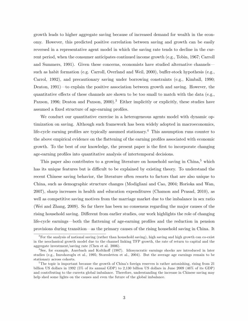
the aggregate household saving rate has increased remarkably since 1992 (see the sold line in

Figure 1), rising from 16.6 percent in 1992 to 27.6 percent in 2007. Data Appendix shows

that using alternative household saving de�nitions reveals equally striking upward trends since

2002, from which the relevant data for computing saving rates become available. The pattern is

also robust to alternative data sources, such as the Flow of Funds Accounts reported in China

Statistical Yearbooks (Yang Zhang and Zhao (2009). Finally, China has been experiencing

dramatic demographic structure change, which might potentially be an important driving

force for the increase in household saving rate.8 To control for demographic characteristics, we

regress household saving rates repeatedly for each cross-section on a child-dependency dummy

(one for households with members below age 16 or having children still attending school and

zero otherwise) and an old-dependency dummy (one for households with retirees and zero

otherwise). The constant terms estimated from the regressions, plotted by the dotted line in

Figure 1, can thus be interpreted as the conditional means of saving rate for households with

no children and retirees. The dotted line demonstrates a pattern similar to the solid line. The

conditional mean increases by 9.5 percentage points, slightly lower than the 11-percentage-point

increase of the aggregate saving rate. Therefore, demographic structure changes only account

for a small share of the increase in Chinese household saving rates. The rising aggregate

saving rates in a fast-growing economy documented above are at odd with the standard life-

cycle/permanent-income models, in which high income growth would naturally result in lower

saving rates for reasons discussed in the introduction.

7Truncating the UHS data at age 80 would give essentially the same result. Quantitatively, it would lowerthe aggregate saving rates by less than one percentage point.

8For instance, the child dependency rate de�ned as whether a household have children below the age 16 orstill attending school dropped from 83.4 percent in 1992 to 66.8 percent in 2007 (see Tabel 1), a trend mainlydriven by the one-child policy. The change of the old dependency ratio is also signi�cant, though less dramatic.It increased from 30.8 percetn in 1992 to 44.4 percent in 2007.

5

[Insert Figure 1]

Panel A of Figure 3 presents age-speci�c saving rates for the two periods 1992-1993 and

2006-2007. Since some age cells contain less limited number of observations, we use three-age

moving average to minimize the e¤ect of measurement error. In the 1992-1993 period, the

saving rates are relatively �at before 45 and then increase towards the retirement age. For the

2006-2007 period, one can see a dramatic change: The saving rate pro�le turns to a U-shape

over the life cycle. Using alternative saving de�nitions result in qualitatively similar U-shape

pro�les (see Data Appendix for details), though the rise of saving rates for age 50-60 may be

less remarkable under certain de�nition. We can further eliminate �xed life-cycle e¤ects by

taking di¤erence of the two pro�les.9 This yields the increase of saving rates over the life cycle

from 1992-1993 to 2006-2007, as depicted in Panel B of Figure 3. The U-shape pattern becomes

more pronounced: The average increase of saving rates for those aged below 40 and above 50

is equal to 11.2 and 10.9 percent, respectively, while that for those middle-aged between 40

and 50 is only 8.3 percent. The rise of saving rate of the young sharply contrasts the typical

hamp-shamped or relatively �at life-cycle saving rate pro�les in mature economies. This is

particularly hard to reconcile with the mainstream thinking that productivity growth leads to

earnings growth for everyone. In that circumstance, the youngest households would have the

lowest saving rate since they face the steepest life-cycle earning pro�le.

[Insert Figure 3]

To see whether the rise of household saving rate has any structural pattern, we investigate

four subsamples classi�ed by household head education and gender. Subsample 1 and 2 include

households with high-school-and-below (non-college henceforth) and college-and-above (college

henceforth) educated household head, respectively. Subsample 3 and 4 include households with

female and male household head, respectively. Figure 4 plots the age-saving pro�les of 1992-

1993 and 2006-2007 for all the four subsamples. The �ndings are immediate. First, the rise of

household saving rate is universal to all subsamples. Second, all subsamples feature a U-shaped

level as well as a U-shaped increase of saving rate over the life cycle.

[Insert Figure 4]

Although the �ndings are qualitatively similar to those from the full sample illustrated by

Figure 3, some quantitative di¤erences are worth mentioning. A comparison between Panel9Life-cycle e¤ects may be time-varing (for instance, the e¤ects of changing age-speci�c household demographic

structures and family structures). See below for an investigation of these time-varing life-cycle e¤ects.

6

A and B shows that the increase of saving rate for college graduates is substantially larger

than that for non-college graduates. From 1992 to 2007, the aggregate saving rate for college

graduates increases by 12.6 percentage points, 2.7 percentage points higher than that for

noncollege graduates. Enhanced by the increasing population share of college graduates and

the widening income gap between di¤erent education groups, the increase of saving rate of

college educated alone can explain more than 40 percent of increase in the aggregate household

saving rate over the sample period. Saving rate of the young (age between 25 and 40) college

graduates is particularly worth being noticed. It increases by XXX percentage points, which

alone contributes to a XXX-percentage-point increase in the aggregate saving rate, about one

third of the rise of the aggregate saving rate over the sample period. If younger and better

educated households could bene�t more from economic growth, their earning pro�les would

be steeper, resulting in lower saving rates accordingly. This observation, therefore, adds extra

burden for theory to match the data. Finally, Panel C and D shows that households with

male household head increase saving rate more than those with female household head. The

aggregate saving rate for the male increases by 11.3 percentage points, about one percentage

points higher than the increase of the aggregate saving rate for the female.

To summary, we have documented the following three main puzzling observations on Chi-

nese household saving rates.

1. The aggregate household saving rate increases remarkably from 1992 to 2007. Moreover,

the increase of household saving rate is an universal pattern: It happens to all groups of

households characterized by age, education or gender.

2. The increase of household saving rate features a U-shape over the life cycle. A similar U-

shaped increase can also be found in di¤erent groups of households classi�ed by education

or gender.

3. Households with college-educated (or male) household head increase their saving rate

more than those with non-college-educated (or female) household head.

2.3 Age-Earning Pro�les

We focus on annual wages for adult workers engaged in wage employment. Wage income

consists of basic wage, bonus, subsidies and other labor-related income from regular job. We

de�ate annual wages to 2007 yuan by province-speci�c urban consumption price indices.10

Our sample for analysis include all workers who are aged 25-55 for females and 25-60 for

10See Data Appendix for detailed descriptions of data sources, variable de�nitions and data adjustments.

7

males, excluding employers, self-employed individuals, farm workers, retirees, students, those

re-employed after retirement, and those workers whose real annual wages were below one half

of the real minimum wage.11

We �rst take a preliminary look at the data by presenting cross-sectional results and then

examine the data statistically. The dotted line in Figure 5 presents the cross-sectional relative

age-earning pro�les in 1992-1993, in which workers of age 42 is used as the reference group to

compute relative earnings. The pro�le features the standard pattern: Earnings increase in age,

reach a peak at 57 and then become rather �at until retirement. China started its transition

towards a full-�edged market economy in the early 1990s. Since then, the earning pro�le has

changed dramatically. The solid line in the �gure presents the cross-sectional relative age-

earning pro�le in 2006-2007. The �attening of the earning pro�les is evident: Workers at age

of 50 earn essentially the same as those at age of 30.

[Insert Figure 5]

Education is a key factor determining labor earnings. In particular, the �attenning cross-

sectional earning pro�les might simply re�ect the fact that the later generations are better

educated and, therefore, earn more than the earlier generations. To control for such an e¤ect,

we classify workers by education and then look at the change of cross-sectional earning pro�le

within each education group. Panel A (B) of Figure 6 depicts age-speci�c earnings for the

group of non-college (college) educated workers relative to earnings at age 42 in the group.

The �attening of age-earning pro�le is also evident in both groups, though less dramatic than

that in the full sample. We then classify workers by gender. Panel C (D) of Figure 6 depicts

age earnings for the group of female (male) workers relative to earnings at age 42 in the

group. Again, age earning pro�les have �attened substantially in both gender groups, though

the �attening occurs at di¤erent life-cycle phases across groups. The age-earning pro�le for

female workers �attens out before age 40, while the �attening of the pro�le for male workers

is signi�cant across all ages.

[Insert Figure 6]

11Provincial-level minimum wages are available only in 2006 from Ministry of Human Resources and SocialSecurity. To impute minimum wages for the previous years, we calculate the ratios of the minimum wages tothe mean wages for each province in 2006. We use the product of these ratios and annual mean wages in eachprovince as our estimates for province-speci�c minimum wages in 1992-2005.

8

2.3.1 Cohort-Based Age-Earning Pro�les

It is well known that cross-sectional pro�les do not necessarily reveal the change in life-cycle

earnings for speci�c individuals over time. The di¤erence between any two cross-sectional

pro�les over time entails both cohort and year e¤ects, while the di¤erence of earnings between

any two ages within a cross-sectional pro�le results from a combination of age and cohort

e¤ects. Because of these potential concerns, we now take an alternative approach: tracing the

earnings of a given cohort of workers by constructing synthetic cohorts. A cohort is denoted

by the year in which individuals turn 25 and enter into our sample. Therefore, individuals

with the same entry year in repeated surveys across periods are treated as being in the same

cohorts.

To examine the changes in the cohort-based earning pro�les, we use the following regression

speci�cation used by Beaudry and Green (2000) and Kambourov and Manovskii (2009).

log y (i; t) = �0 + �1z (i) + �2z (i)2 + �3z (i)x (i; t) (1)

+�1x (i; t) + �2x (i; t)2 + �3x (i; t)

3 + �4 log Y (t) + " (i; t) :

Here, the dependent variable, y (i; t), is the log annual earnings for a given cohort i in a given

year t. The regressors include the cohort entry year, z (i), and its square, an interaction of

age, x (i; t), and the cohort entry year, plus a polynomial of age.12 To control for the e¤ects

of aggregate earnings shocks on individual earnings, we introduce log detrended aggregate

earnings, log Y (t), as an additional regressor.13 More speci�cally, Y (t) = Y (t) =Y0 (1 + g)t,

where we choose g = 6:7% such thatPt log Y (t) = 0. Since the sample contains 36 ages and

16 years, we have a total of 576 observations.

[Insert Table 2]

The estimated results are reported in Column (1) of Table 2. The large and positive

coe¢ cient on the linear cohort term, �1, shows that the younger cohorts earn substantially

more than the older cohorts. The negative coe¢ cient on the quadratic cohort term, �2, on

the other hand, suggests that the earnings gap across cohorts is narrowing over time. The

rise in earnings across successive cohorts is clearly an important reason for the �attening of

the cross-sectional pro�les in Figure 5. These �ndings are in line with Modigliani-Paxson�s

postulation on the change of life-cycle earnings in a growing economy (e.g. Modigliani, 1986;

12Following Beaudry and Green (2000), the �rst cohort with entry year of 1957 in our sample is indexed bycohort 1. The following successive cohorts are counted up incrementally.13Beaudry and Green (2000) use unemployment rates, which are actually �at and not informative in China.

9

Paxson, 1996); i.e., aggregate growth manifests itself in a rapid shift upward of the level of age

earning pro�le from cohort to cohort. These estimates imply an average annual growth rate

of 8:6% for starting earnings at age 25 over the sample period, higher than the growth rate of

7:5% for aggregate earnings. The key coe¢ cient on the age-cohort interaction, �3, is negative

and highly signi�cant. This result suggests that the later cohorts face �atter earning pro�les

and, thus, lower earnings growth over the life cycle than the earlier cohorts. Such an e¤ect is

quantitatively large. For the 2007 cohort, our estimates imply that their earnings would grow

at an average annual rate of 5:0% over the life cycle, substantially lower than the rate of 7:1%

for the 1992 cohort.

As a robustness check, we replace detrended aggregate earnings, log Y (t), with year dum-

mies. In this case, an identi�cation condition is needed since cohort, age and year are a linear

combination of each other. Following Deaton and Paxson (1994), we add two restrictions such

that (i) year dummy coe¢ cients sum up to zero; (ii) year dummy coe¢ cients are orthogonal to

a time trend. Column (2) reports the estimated results. The coe¢ cient of interest, �3, remains

negative and highly signi�cant, though the absolute value drops from 0:0011 to 0:0008. All the

other estimates are essentially the same as those in Column (1).

The Chinese government started reforming the central-planned economy in 1978. Therefore,

cohorts entering into labor market after the reform might have age-earning pro�les di¤erent

from earlier cohorts. To isolate age-earning pro�les of �lucky generations,�we run the same

regressions for a subsample of cohorts with entry years later than 1978 only. The subsample

contains 376 observations, less than two-third of the full sample. The results are presented by

Column (3) and (4). The estimated �3 is still negative in both columns and remains highly

signi�cant in Column (4).

The speci�cation (1) can easily be extended to estimate group-speci�c cohort-based age-

earning pro�les.

log y (i; j; t) = �0 (j) + �1 (j) z (i) + �2 (j) z (i)2 + �3 (j) z (i)x (i; t) (2)

+�1 (j)x (i; t) + �2 (j)x (i; t)2 + �3 (j)x (i; t)

3 + �4 (j) log Y (t) + " (i; j; t) ;

where y (i; j; t) denotes the earnings of individuals with age i and group j at period t. Column

(1) to (4) in Table 2 report estimation results for groups of non-college-educated, college-

educated, female and male workers, respectively. Interestingly, the estimated �3 changes con-

siderably across groups. Despite negative in all groups, �3 is highly signi�cantly only for

college-educated or male workers. The estimated absolute value of �3 in these two groups

(0:0019 for the college-educated and 0:0014 for the male) is also much larger than their coun-

10

terparts in the other two groups (0:0008 for the non-college-educated and 0:0001 for the female).

The �attening of cohort-based age-earning pro�les is particularly remarkable for the college-

educated. For the 2007 cohort, their annual earnings growth rate over the life cycle is 4:2

percent, nearly half of the rate of 7:9 percent for the 1992 cohort.

[Insert Table 3]

The estimate for �4 (j) also features substantial heterogeneity across education groups. It

varies from 0:90 and 0:84 for the non-college educated and the female, respectively, to 1:11 and

1:16 for the college-educated and the male, respectively. These estimates imply that earnings

of the college-educated and the male tend to be more volatile over the business cycle. This

might provide an explanation, through precautionary saving motives, for higher saving rates

of the college-educated and the male, complementary to our explanation provided below. We

will leave it as an interesting extension for future research.

Beaudry and Green (2000) and Kambourov and Manovskii (2009) �nd similar patterns of

the �attenning life-cycle earning pro�les in Canada and U.S. Nevertheless, the �attening of

the pro�les in China is, on average, more prominent. For instance, Kambourov and Manovskii

(2005) report an estimated �3 of �0:004 in the PSID data, with a magnitude much smaller thanthe one in column (1) of Table 2. Beaudry and Green (2000) document a strong �attenning of

the earning pro�les for high-school educated men in Canada. However, the overall picture is

less clear as �3 becomes statistically insigni�cant for university educated men and high-school

educated women and even turn positive for university educated woman.

2.4 Pension

We now turn to the Chinese pension system. Pensions are not only theoretically relevant, but

empirically important for saving decision over the life cycle (e.g. Attanasio and Brugiavini,

2003). The documentation of pension system also sheds light on the following quantitative

exercises. We shall use a combination of earning pro�les and a replacement rate, the key

variable measuring the generosity of a pension system, to provide a full characterization of

workers�non-asset income over the life cycle.

The Chinese pension system, which has undergone a series of reforms since the early 1990s.

The original system was primarily based on state and urban collective enterprises in the central-

planned economy. All pension bene�ciaries received generous pension bene�ts directly from

their employers. The actual replacement rate can be as high as 80 percent (see, e.g., OECD,

2007 and Figure A-1 below). The work-unit-based system was under severe �nancial distress

11

in the late 1980s and early 1990s, mainly due to a growing disproportion between the numbers

of contributors and bene�ciaries (Zhao and Xu, 2002). To deal with the issue, the government

has initiated a transition from the traditional Pay-As-You-Go system (PAYGO henceforth) to

a partially-funded one since the early 1990s. A new system was implemented after the State

Council issued �A Decision on Establishing a Uni�ed Basic Pension System for Enterprise

Workers (Document 26)�in 1997.

The reformed system consists of three pillars. The �rst pillar, funded by 17 percent wage

taxes paid by enterprises, guarantees a replacement rate of 20 percent of local average wage

for retirees with a minimum of 15 years of contribution. The second pillar provides pensions

from individual accounts �nanced by a contribution of 3 and 8 percent wage taxes paid by

enterprises and workers, respectively. The third pillar adds to individual accounts through

voluntary contribution. The return of individual accounts would be adjusted according to

bank deposit rates. The system also de�nes monthly pension bene�ts from individual account

equaling the account balance at retirement divided by 120. The targeted replacement rate of

the system is 58.5 percent. Suppose that wage growth rate is equal to the interest rate. For a

worker contributes to the system for 35 years (from age 25 to 60), her pension bene�ts should

be equal to 20 percent of average wages (the �rst pillar) plus 38:5 percent of her wage before

retirement.

More recently, a new reform was implemented after the State Council issued �A Decision

on Improving the Basic Pension System for Enterprise Workers (Document 38)�in 2005. The

reform adjusted the proportion of taxes paid by enterprises and individuals and the proportion

of contribution for individual accounts. Now individual accounts are funded by wage taxes of

8 percent paid by workers only. Moreover, the reform changed pension bene�ts substantially.

The replacement rate of an individual is entirely determined by years of contribution: One

year contribution increases the replacement rate of an wage index averaged from local and

individual wages by one percentage point.14

Although the generosity of the Chinese pension system has been reduced dramatically

through these reforms, a targeted replacement rate close to 60 percent still stands high and is

actually higher than the rate in most OECD countries (OECD, 2007).15 However, the actual

replacement rate could be much lower. One of the main problems of the current system is the

widespread payment evasion. To reduce pension contributions, enterprises have the incentive of

14The article, however, did not state explicitly how to compute the wage index.15The new reform of 2005 announced a targeted replacement rate of 59.2%. Although the rate is 0.7 percentage

points higher than the target of 1997, the actual replacement rates decline dramatically (e.g. Lin and Ding,2007).

12

reporting lower wages. The system requires a contribution rate of 20 percent from enterprises,

while the actual rate is about 5 percent according to the enterprise survey conducted by NBS

(see Li and Wu, 2010). The under-reported wage bill leads to a lower actual payroll tax rate

paid by individual workers. Our UHS data reveal an average contribution rate of 4.1 percent

from 2002 to 2007, about half of the o¢ cial rate. Therefore, a balanced pension system would

imply pension bene�ts of 5 percent of average wages from the �rst pillar. Suppose, again, that

wage growth rate is equal to the interest rate. For a worker contributes to the system for 35

years, the second pillar would provide pension bene�ts equaling 14 percent of her wage before

retirement. In other words, the actual replacement rate is 19 percent, only one-third of the

targeted rate.

We next present a quantitative assessment on the evolution of the Chinese pension system.

Due to the lack of data on historic earnings, actual replacement rates are hard to obtain.

Instead, we compute the aggregate replacement rate as a percentage of average pensions per

retiree over average wages per worker. Chinese Statistical Yearbook (CSY) reports �Pensions

for Retired and Resigned Persons per capita� up to 2005. We then divide this variable by

�Average Wage of Sta¤ and Workers�to generate a proxy for the aggregate replacement rate.

The solid line in Figure 7 plots the results from 1992 through 2005. The aggregate replacement

rate was above 80 percent in early 1990s, consistent with the impressionistic view that the

original work-unit-based pension system entails generous inter-generational redistribution. The

pension reform in 1997 cut pension bene�ts substantially for those newly retired workers,

driving the aggregate replacement rate to fall in late 1990s. The declining trend continues

in the 2000s. The aggregate replacement rate dropped to 58 percent in 2005. Dunaway and

Arora (2007) report a similar but less dramatic pattern. They show that the replacement rate

of average manufacturing wages declined from 82 percent in 2000 to 68 percent in 2005.

[Insert Figure 7]

Aggregate replacement rates may be overestimated due to misreported wage bills. We

then use pensions data in UHS as an alternative measure. Since 2002, UHS has adopted

a new de�nition of pension that covers a lot more items other than the narrowly-de�ned

pension, such as the reimbursement of medical expenditure from enterprises and the public

health care system. To maintain the data consistency, we only compute aggregate replacement

rate, as a ratio of average pensions per pension bene�ciary over average earnings per worker,

for the period 2002 to 2007. The results are plotted by the dotted line in Figure 7. The

aggregate replacement rate from UHS also features a downward trend, declining from 61.8

13

percent in 2002 to 52.4 percent in 2007. Two addition remarks are in order. First, the aggregate

replacement rate from UHS overestimates the actual rate since the new de�nition of pension

in UHS contains many items other than pension bene�ts. Second, though overestimated, the

aggregate replacement rate from UHS is still signi�cantly lower than that from CYS. In 2002,

for instance, the rate from UHS equals 61.8 percent, about 10 percentage points below that

from CYS. This is in line with the fact that enterprises under-report wage bills.

3 A Four-Period OLG Model

We have shown dramatic changes in life-cycle earning pro�les in China over the period asso-

ciated with fast economic growth. The cohort e¤ects on starting earnings and the �attening

of the earning pro�les are particularly remarkable. We now formulate a life cycle model to

study how these changes a¤ect household saving rate as well as their patterns of life-cycle

saving. We �rst use a four-period OLG model with simple analytical results to make the un-

derlying mechanism highly transparent. A full-�edged Auerbach-Kotliko¤ OLG model will be

presented in the next section, in which the observed life-cycle earning pro�les are imposed to

deliver quantitative results.

The economy is populated with four overlapping generations with equal mass, referred to

as the young, middle-aged, old workers and the retired. In each period, all workers supply one

unit of labor inelastically. The after-tax earnings of the young, middle-aged and old at period t

are denoted by w1t , w2t and w

3t . The retirees at period t receive pensions of pt, which is equal to

tYt, where t and Yt represent the replacement rate and average earnings. We abstract away

from taxes and, thus, how pensions are �nanced. Alternatively, we may introduce a balancing

government budget, allowing the tax rate to be endogenously determined by pensions. Such

an extension would lead to no major change to our main results.

Preferences for a young individual born at period t are represented by

4Xi=1

�i�1u�cit+i�1

�; (3)

where u (�) is a standard twice di¤erentiable and strictly concave utility function, � denotes thediscount factor, and cit stands for consumption of an individual of age i at period t. The young

individual chooses the optimal saving decision by maximizing (3) subject to her intertemporal

budget constraint:

4Xi=1

cit+i�1

(1 + r)i�1=

3Xi=1

wit+i�1

(1 + r)i�1+

pt+3

(1 + r)3;

14

where r is the interest rate and pt = tYt � tPiw

it=3. Denote a

it the asset of age i at the

beginning of period t. Individuals are born with no assets; i.e., a1t = 0.

For expositional ease, we restrict our attention to the case with � = 1+ r = 1, in which the

Euler equation implies equalized consumption �ow over the life time. In the technical appendix,

which is available from our website, we relax the assumption and show that our main results

are robust to a large set of parameter values. Moreover, to focus on the role of earnings

pro�les, we assume away within-cohort heterogeneity and let t = 0 8t in the benchmark forsimplicity. These assumptions will be relaxed below, to understand how changes in group-

speci�c age earnings pro�le and replacement rates in�uence the aggregate saving rate as well

as the increase of saving rates over the life cycle.

The assumption � = 1 + r = 1 implies the following life-cycle saving rate pro�les:

sr1t =3

4� 14

�w2t+1 + w

3t+2

w1t

�; (4)

sr2t =3

4� 14

�w1t�1 + w

3t+1

w2t

�; (5)

sr3t =3

4� 14

�w1t�2 + w

2t�1

w3t

�; (6)

where t � T and srit denotes the saving rate of age i at period t. These results are straight-

forward and standard. In particular, (4), (5) and (6) show that saving rates increase in the

current earnings and decrease in the past and future earnings. In other words, the life-cycle

saving rate pro�le appears to �track�the earnings pro�le for consumption smoothing.

3.1 Growth and the Rise in Saving Rate

Consider an economy on a balanced-growth path such that Yt+1 = (1 + g)Yt and wi+1t+1 =

(1 + g)wit, where g is the steady state earnings growth rate. (4) and (5) determine the following

steady state asset-earnings ratios:

a2tw2t

=3= (1 + g)� (2 + g)

4; (7)

a3tw3t

=

�1= (1 + g)2 + 1= (1 + g)

�� 1

2: (8)

Here, a2t and a3t denote assets of the middle-aged and the old at the beginning of period t,

respectively. We assume a su¢ ciently small g so that a2t > 0 and a3t > 0.

A unanticipated change occurs at the beginning of period T such that

wiT > wiT ; (9)

15

where wit stands for earnings of workers with age i at period t � T after the change occurs

at period T . According to (9), the change yields earnings are higher than the anticipated

earnings wiT , implying a unanticipated earnings growth at period T . Echoing the acceleration

of economic growth in China after 1992, we assume

Yt+1 > (1 + g)Yt; t � T; (10)

where Yt denotes average earnings after the change occurs. In other words, future aggregate

earnings also grow at a faster rate than g in the original steady state. We shall see below that

under the assumption (10), a representative agent model would predict a fall of saving rate at

period T .

To understand how a �attening of age earnings pro�les a¤ect saving decision, we assume

that earnings growth at the aggregate level translates into the following individual earnings

growth:w2T+1w1T

< 1 + g;w3T+2w2T+1

<w3T+1w2T

< 1 + g: (11)

(11) shows the �attening of age earning pro�les, which is in line with the empirical �ndings in

Table 1 and 2. Despite highly hypothetical, (9) and (11) capture, in a broad sense, the stylized

features of earnings pro�les we observe from the fast-growing economy of China described in

Section 2.3.

De�ne �srit � srit� srit�1 the increase of saving rate of age i over period t and t�1. Whenthe unanticipated earnings growth arrives at period T , we have

�sr1T =1

4

(1 + g)�

w2T+1w1T

!+1

4

(1 + g)2 �

w3T+2w1T

!| {z }

e¤ect of �attening pro�le

> 0: (12)

The inequality in (12) comes from (11). The �attening of age-earning pro�le raises the rel-

ative earnings of workers when they are young. Their saving rate increases accordingly for

consumption smoothing. We refer this change in saving as the e¤ect of �attening earning

pro�le.

The increase in saving rate of the middle-aged is equal to

�sr2T =a2T3w2T

�1� w2T

w2T

�| {z }

e¤ect of earning growth

+1

3

(1 + g)�

w3T+1w2T

!| {z }e¤ect of �attening pro�le

> 0; (13)

respectively, where a2T =w2T follows (7). The inequality in (13) comes from (9) and (11). Com-

paring with the middle-aged at the original steady state, the period-T middle-aged would like to

16

increase their saving rate for two reasons. First, their current earnings, w2T , is higher than their

anticipated earnings, w2T�1. Holding constant the age-earning pro�le, this change, referred to

as the e¤ect of earning growth, raises their saving rate. Second, since the middle-aged antici-

pates a �attened age-earning pro�le, i.e., (1 + g)� (w3T+1=w2T ) > 0; there is a positive e¤ect ofage-earning pro�le similar to that in (12), which yields a higher saving rate.

Finally, �sr3T can be written as

�sr3T =a3T2w3T

�1� w3T

w3T

�| {z }

e¤ect of earning growth

> 0; (14)

where a3T =w3T follows (8). The inequality in (14) comes from (9). The old at period T increase

their saving rate simply because they earn more than their ancestors. The e¤ect of age-earning

pro�le does not apply to the old since they do not receive labor earnings after retirement.

This highly stylized four-period model illustrates two main implications from the �attening

of age earnings pro�les. First, �sriT > 0 for all i implies that �srT > 0; i.e., the aggregate

saving rate increases when the economic growth accelerates at period T .16 This sharply con-

trasts the prediction of the representative agent model. Anticipating future income growth as

in (10), the representative agent would like to borrow from the future, resulting in a fall in the

saving rate at period T .

Second, consider the case in which a2T is su¢ ciently low and w3T+1=w

2T is su¢ ciently large,

while a3T is su¢ ciently large and w3T+2=w

2T+1 (or w

2T+1=w

1T ) are su¢ ciently low. Then, �sr

1T >

�sr2T and �sr3T > �sr

2T . In other words, a simple model with forward-looking rational agents

has the ability of generating a U-shaped increase of saving rate over the life cycle as observed.

The intuition of these conditions is straightforward. A low a2T (a high a3T ) dampens (ampli�es)

the e¤ect of current earnings for the middle-aged (old). A high w3T+1=w2T and a low w

3T+2=w

2T+1

imply that the �attening of age-earning pro�le is more pronounced for the later cohort. Both

of the conditions can be justi�ed on theoretical and empirical basis. The larger asset position

of the old is a natural outcome of the life-cycle model. Empirically, our UHS data show that

the average deposit to earnings ratio for workers between age 50 and 60 is about two times

higher than that for workers between age 40 and 50 in 1992. Section 2.3 provides empirical

evidence for the �attening age earnings pro�les cohort by cohort. We shall see in Section 4 that

a full-�edged quantitative model with the observed age earnings pro�le changes can match the

observed U-shaped increase of saving rate over the life cycle.

16 Including dissavings of the retirees from aggregate savings would lead to the same result since their dissavingsremain unchanged from period T � 1 to T .

17

3.1.1 Two Extensions

We have shown that a �attening of age earnings pro�le can explain the �rst two empirical

facts documented in Section 2.2. We now extend the above framework to incorporate within-

generation heterogeneity, to shed some lights on the third empirical fact. Denote wijt the

wage of an individual of age i with education level j. The assumptions of (9) and (11) are

maintained for all j. Without loss of generality, we let wijt be increasing in j. If j refers

to education levels, the increasing wijt would capture the return to education. We further

assume that wijT =wijT is increasing in j, while w2jT+1=w

1jT , w

3jT+2=w

1jT and w3jT+1=w

2jT are all

decreasing in j. The increasing wijT =wijT implies a faster earnings growth as j increases. The

decreasing w2jT+1=w1jT , w

3jT+2=w

1jT and w3jT+1=w

2jT imply a more pronounced �attening of age-

earning pro�les as j increases. These assumptions re�ect the empirical observations reported in

Table 3 in Section 2.3.1. The larger cohort and age e¤ects in Column (2) and (4) suggest that

college graduates and male workers have a higher wijT =wijT than their counterparts. Moreover,

age-earning pro�les of college graduates and male workers turn �atter than those of their

counterparts according to the larger absolution value of the age-cohort interaction coe¢ cient.

Under these assumptions, the model would predict an increasing �sijT in j, which is consistent

with the third empirical fact on Chinese household saving rates.

Another important extension is to introduce a pension system. The facts presented in

Section ?? suggest a sharp declining trend of replacement rates since the middle of 1990s

when the pension reform was implemented. We let t = for t < T and then introduce an

unanticipated change to the pension system such that the replacement rate starts to fall from

period T and on, with t+1 � t � for t � T . A su¢ ciently large fall of the replacement

rate, together with a modest increase in future earning growth, would lower future pension

bene�ts for all cohorts at period T . In this case, the saving rates would shift upwards further.17

3.2 Myopic Expectation

So far we have implicitly assumed that individuals hold perfect foresight on their future earnings

after the economy takes o¤ at period T . Although theoretically appealing, perfect foresight

might be far from the way individuals form their expectations in a rapidly-changing economy

like China. With a former central-planned economy transformed into a rather sophisticated

market economy in less than two decades, information about future earnings must be limited,

while past information quickly becomes obsolete. Individuals, therefore, may naturally rely

17 If, instead, earnings grow much faster that the original balanced-growth path, future pension bene�ts wouldgrow as well. Then, the sign of �sriT may turn ambiguous. The algebra is straightforward and thus omitted.

18

more on current information to form expectations. In fact, a number of studies have even found

empirical evidence supporting myopic behavior in developed economies. Reimers and Honig

(1996) provides an example. They show that male workers in the U.S. respond only to current

pension bene�ts and do not take into account changes in future bene�ts. For these concerns,

this subsection adopts myopic expectation, as a robustness check for our above �ndings.

Throughout the paper, we refer to myopic expectation as the case in which individuals use

the current cross-sectional age earnings pro�le to forecast their future earnings. More precisely,

denote Et�wit+k

�the myopic expectation on wit+k at period t, we have

Et�wit+k

�= wit: (15)

In addition, individuals form myopic expectation on the replacement rate in a consistent way:

Et� t+k

�= t: (16)

Following the cross-sectional evidence on the �attening of age-earning pro�le in Figure 5,

we assume

w2Tw1T

< 1 + g;w3Tw2T

< 1 + g: (17)

From (17), it is immediate that

�sr1T =1

4

�(1 + g)� w2T

w1T

�+1

4

�(1 + g)2 � w3T

w1T

�| {z }

e¤ect of �attening pro�le

> 0; (18)

�sr2T =a2T

3w2T�1

1�

w2T�1w2T

!| {z }e¤ect of earning growth

+1

3

�(1 + g)� w3T

w2T

�| {z }e¤ect of �attening pro�le

> 0: (19)

Here, we abstract away within-cohort heterogeneity and pension for simplicity. The increase of

saving rate of the old under myopic expectation is identical to (14) since expectation becomes

irrelevant for them. Despite di¤erent ways of forming expectations, (18) and (19) delivers

essentially the same results as (12) and (13). The reason is simple: The cross-sectional age

earnings pro�les also feature a �attening process similar to the cohort-based pro�les. Therefore,

the age saving pro�les will shift upwards irrespective of perfect foresight or myopic expectation.

Therefore, the main �ndings stated above are robust to alternative schemes of expectations.

We may further extend the model by introducing within-cohort heterogeneity and pension in

a way similar to those under perfect foresight. The results are obvious and, hence, omitted.

19

We have shown that in a highly stylized life cycle framework, more starting earnings,

together with a �attening of age earnings pro�le, can not only increase the aggregate saving

rate, but result in a U-shape increase of saving rate over the life cycle. Moreover, the increase of

saving rate is larger for individuals experiencing a more pronounced �attening of the earnings

pro�le. In the next section, we shall turn to a more sophisticated model, to assess quantitatively

how observed changes to earnings pro�les in China would a¤ect household savings at the

aggregate level and over the life cycle.

4 A Full-Fledged OLG Model

In this section, we incorporate changes in age earnings pro�les observed from China to an

otherwise standard life-cycle model. Our aim is to assess quantitatively the extent to which

the observed facts can explain the Chinese household saving puzzle over the period 1992 to 2007

(including the surge of the aggregate household saving rate as well as the U-shaped increase

in saving rates over the life cycle). Given such a goal, the foregoing four-period OLG model,

which corresponds one period to twenty years, would be inadequate. Therefore, we extend the

model to a full-�edged OLG model in which one period corresponds to one calendar year and

individuals live up to 75 periods after entering the labor market.

Individuals start working at age 1 and retire at age Tr. Each individual receives an en-

dowment of human capital at birth, and supplies one unit of labor inelastically in each period.

We use wijt to denote the after-tax earnings of an individual of age i with endowment j at

period t. Similarly, pijt stands for the pensions of a retiree of age i with endowment j at period

t. Length of life is uncertain. Let �i denote the unconditional survival rate up to age i, with

�1 = 1. The survival rate conditional on being alive at age i� 1 is thus equal to �i=�i�1.

4.1 Perfect Foresight

To compute individuals�optimal saving rates, we need to specify how expectations on future

earnings are formed. There are two alternative approaches in the literature of life cycle analy-

sis: adopting either perfect foresight (e.g. Auerbach and Kotliko¤, 1987) or myopic expectation

(e.g. Davies and Whalley, 1991). In this subsection, we assume that, as in the four-period

model, individuals hold perfect foresight on their earnings, which are drawn from the esti-

mated cohort-based age earnings pro�les.18 We will turn to an alternative myopic expectation

approach below as a robustness check.

18 Individuals can also foresee perfectly the evolution of demographic structures to form expectations on theirpension bene�ts.

20

Preferences for an individual of age i = n with endowment j are represented by

TXi=n

�i�i�nu�cijt+i�n

�; (20)

where �i � �i�=n�� and �� denotes the subjective discount factor at age � . We allow age-

speci�c discount factor to incorporate life-cycle elements a¤ecting saving decision. In par-

ticular, �� will be calibrated to match the age saving rate pro�le in 1992. The individual

worker chooses the optimal saving decision by maximizing (20) subject to the following budget

constraint:

TXi=n

cijt+i�n

(1 + r)i�n= I

TrXi=n

wijt+i�n

(1 + r)i�n+

TXi=Tr+1

pijt+i�n

(1 + r)i�n

!(21)

+(1� I)TXi=n

pijt+i�n

(1 + r)i�n+ (1 + r) aijt ;

where I is an indicator function with I = 1 for n � Tr and I = 0 otherwise, and aijt denotes

asset position of an individual with age i and endowment j at period t.

Following the documentation of the Chinese pension system in Section ??, we assume

a pension system as a mixture of Document 26 and Document 38, adjusted by the actual

contribution rates. Speci�cally, by Document 26, annual pension bene�ts are equal to a sum

of 20 percent of average wages (the �rst pillar) and the individual account balance at retirement

divided by 10 (the second pillar). By Document 38, workers contribute 8 percent of earnings

to their individual accounts. The return to individual accounts is equal to the interest rate, r.

For notational convenience, we de�ne

Yt �Xi

Xj

� (i; j; t)wijt (22)

as the average wages at period t, where � (i; j; t) denotes the population density for age i group

j at period t. In addition, de�ne

W ijt � 1

Tr

t�i+TrX�=t�i+1

R��(t�i+1)wj� (23)

as the average lifetime earnings of workers j born at t� i+ 1. Then, pension bene�ts can be

written as

pijt = �1 � 20% � Yt + �2 � 8% �W ijt �

Tr

10; (24)

where �1 and �2 denote adjustment rates for the �rst and second pillars, respectively, according

to actual contribution rates.

21

Denote srijt the saving rate of individuals with age i and type j at period t. The aggregate

saving rate can be computed by aggregating individual saving rates over i and j:

srt =

PTri

Pj � (i; j; t) sr

ijt w

ijtPTr

i

Pj � (i; j; t)w

ijt

: (25)

To be consistent with the data, we exclude saving rates of the retirees. The cross-sectional

life-cycle saving rate pro�le at period t consists of the average saving rates of individuals of

age i 2 [1; T r]:

srit =

Pj � (i; j; t) sr

ijt w

ijtP

j � (i; j; t)wijt

: (26)

4.1.1 Benchmark Parameterization

Agents enter the economy at age 25 and live until 100 (N = 76). Let Tr = 36 as the

retirement age for male workers in China is 60. The annual interest rate is set to 3%, which

is slightly higher than government bond returns in the period 1992-2007 but much lower than

stock market returns over the period. We assume log preference so that the intertemporal

elasticity of substitution is equal to one. The survival rates are obtained by the actual age-

conditional survival rates from the 2005 population consensus (China Statistical Yearbook,

2006). The population density, � (i; j; t), follows the actual density in the UHS data. We let

� (i; j; t) = � (i; j; 2007) for t > 2007.

The age-speci�c discount factors, �i, are calibrated to match the initial age-saving pro�le.

Since saving rates of retirees are excluded, we simply let �i = �Tr for i > Tr. Then, �Tr is

chosen such that the initial saving rate for workers at retirement age is equal to that in the

data. �i for i < Tr can thus be calibrated in a recursively way. Figure A-1 in the appendix

plots the calibrated age discount factors, with a mean of 0:978.

Section ?? has presented the evidence of low actual contribution rates to the pension

system. In particular, enterprises only contribute 5 percent of wages, only one-fourth of the

o¢ cial rate. We then set the adjustment rate for the �rst pillar, �1, equal 0:25. Similarly, since

the actual contribution rate of workers is about half of the o¢ cial rate, �2 is set to 0:5.

Most importantly, age-earning pro�les follow (1), with �4 = 0 and all other coe¢ cients

being equal to the estimates in column (1) of Table 1. In other words, we abstract away

within-cohort heterogeneity in the benchmark parameterization. �4 = 0 is observationally

equivalent to remove aggregate earnings shocks in this economy. The estimated coe¢ cients

are also used to predict future earnings after 2007. The out-of-sample projection suggests the

economy would continue to grow for years to come: The predicted aggregate earnings growth

22

rate is above 5 percent until 2038. Pension bene�ts are computed by according to (24), (22)

and (23). Since we do not have complete life-time earnings data for those who enter into labor

market before 1992, only the predicted earnings after 1992 are used to compute their average

life-time wages.

Finally, we assume the following initial age asset distribution. The asset-earnings ratio

starts from zero at age 25, peaks at the age of retirement and falls to zero at the end of life.

Further, the asset-earnings ratio changes in a linear way:

ai1wi1

=

8<:i�1Tr�1 �

aTr1wTr1

T�iT�Tr�1 �

aTr1wTr1

if i � Trotherwise

: (27)

We set the peaked asset-earnings ratio, aTr1 =wTr1 , to 4, roughly consistent with the deposit-

earnings ratio for workers with age between 55 and 60 in 1992.

4.1.2 Results

The aggregate saving rate, srt, is plotted in Panel A of Figure 8. Solid and dotted lines

represent the simulated results and actual data, respectively. The model predicts a take-o¤ of

aggregate saving rate since 1992, with a trend similar to that in the data. Note that subjective

discount factors are chosen to match the initial saving rates over the life cycle and, hence,

the initial aggregate saving rate. However, the dynamics of aggregate saving rate is entirely

endogenous. The rise of saving rate is quantitatively large. The aggregate saving rate increases

by 9:2 percentage points, only 1:8 percentage points lower than the increase in the data. Panel

B displays the increase of saving rate over the life cycle, sri2007 � sri1992. Consistent with the

argument in Section 3, the model indeed features a U-shaped increase of saving rate over the

life cycle. The model (solid line) matches the data (dotted line) reasonably well until age 45.

Nevertheless, the simulated increase of saving rate above age 45 is too small.

[Insert Figure 8]

We then allow within-cohort heterogeneity by introduce di¤erent education endowments

at birth. Let j 2 fH;Cg, representing high-school-and-below and college-and-above educatedindividuals. Their age earnings pro�les follow (2), with �4 (j) = 0 and all the other coe¢ cients

being equal to estimates in Column (1) and (2) of Table 2. We maintain the initial asset-

earnings ratios in the benchmark parameterization for both non-college and college graduates

but recalibrate �i to match the initial saving rates over the life cycle. This yields a mean of �i

of 0:971. The dashed lines in Figure 8 plot the simulation results. Interestingly, the simulated

23

aggregate saving rate increases by 10:2 percentage points, one percentage point higher than

that of the benchmark model with no within-cohort heterogeneity. This is primarily because

college graduates increase their saving rate much more than non-college graduates. The average

gap amounts to 8 percentage points over the life cycle. Much of the gap, in turn, is driven by

the more �attened age earnings pro�les for college graduates. The key coe¢ cient, �3, is equal

to �0:0019 for college graduates, more than doubled than that for non-college graduates.Moreover, the dashed line in Panel B shows that introducing within-cohort heterogeneity

improves substantially the �tness for the increase of saving rate over the life cycle. In particular,

the extended model predicts much higher increases of saving rate above age 45. This is, again,

led by college graduates.

Now, we check the parameter sensitivity of the above �ndings. First note that by calibrating

age-speci�c discount rates, �i, to match the initial saving rates over the life cycle, intertemporal

elasticity of substitution would have no e¤ects on the increase of saving rates. Changing � only

leads to di¤erent calibrated values of �i. For instance, lowering � from 1 to 0:5 yields a mean of

recalibrated �i of 0:96. So we analyze sensitivity to the remaining three key parameters: (i) the

initial asset-earnings ratio aTr1 =wTr1 ; (ii) the adjustment parameters of the pension system, �1

and �2. Speci�cally, we use the extended model as the benchmark case and perturb one of the

parameters in each of three experiments. In the �rst experiment, we increase aTr1 =wTr1 from 4

to 5, to match the long-run asset-earnings ratio. Since the pension system does not necessarily

run self-balanced budget, the actual contribution rates might under-estimate the replacement

rates. Therefore, the second and third experiments increase �1 and �2 by half, respectively.

The results are plotted in Figure 9. It can be seen that our main �ndings are robust to these

alternative parameterizations. In fact all the experiments lead to a larger increase of aggregate

saving rate.

[Insert Figure 9]

Our quantitative analysis shows that, once incorporating the observed changes in earnings

pro�les, an otherwise standard life-cycle model can account well for the recent surge in house-

hold saving as well as the U-shaped increase in saving rates over the life cycle. However, it is

also worth pointing out that the model is less successful in matching the rise of saving rate

for age between 50 and 60. Note that the model presented above is very simple and abstracts

away household characteristics. The �tness could be improved if adjustments are made for

controlling the e¤ects of family structure (see Section (4.3) for details).

24

4.2 Myopic Expectation

This subsection adopts myopic expectation as an alternative approach. In the context of the

present paper, following (15), myopic expectation is referred to as the case in which individuals

use the current cross-sectional life-cycle earnings pro�le to forecast their future earnings. In

other words, everyone expects that the current cross-sectional life-cycle earnings pro�le will

remain unchanged inde�nitely. Consequently, any change to the pro�le in the future will be

perceived as an unanticipated permanent change.

We further assume that individuals hold myopic expectation on pension bene�ts; i.e., they

expect future their pension bene�ts to be the same as pension bene�ts for current retirees.

The myopic expectation on pension bene�ts follow

Et

hpijt+i�n

i= pijt : (28)

Individuals can in principle form forward-looking expectations on their pensions by perceiving

payment rules of the system. However, as discussed in Section ??, the Chinese pension system

has undergone a series of reforms, transiting from a original work-unit-based system to the

current PAYGOmixed with individual accounts. The associated dramatically changing pension

bene�ts provide additional justi�cation for the myopic expectation in (28).19

Finally, we assume current pension bene�ts are evenly distributed across retirees and equal

to the average wages multiplied by the aggregate replacement rate:

pijt = � � t � Yt: (29)

We know that the observed aggregate replacement rates in Figure 7 overestimate the generosity

of the pension system. So the adjustment parameter, �, is introduced to correct the potential

inconsistency.

4.2.1 Parameterization

Following the same procedure, we calibrated the age-speci�c discount factors, �i, to match

the initial age-saving pro�le. The mean of �i is equal to 0:966. Let wijt and t be equal to

the observed earnings and aggregate replacement rates. As before, we consider two model

economies. The �rst model has no within-cohort heterogeneity, where wijt equals the average

wage of age i, and the second one introduces di¤erent education endowments. The initial

asset-earnings ratios still follow (27), with aTr1 =wTr1 = 4. � is set to 1 in the benchmark case.

19Michaud and van Soest (2006) show that even in the U.S., workers tend to misperceive the complicatedrules of the social security system.

25

We will show below that the main results are robust to di¤erent values of �. All the other

parameter values are identical to those in Section 4.1.1 under perfect foresight.

4.2.2 Results

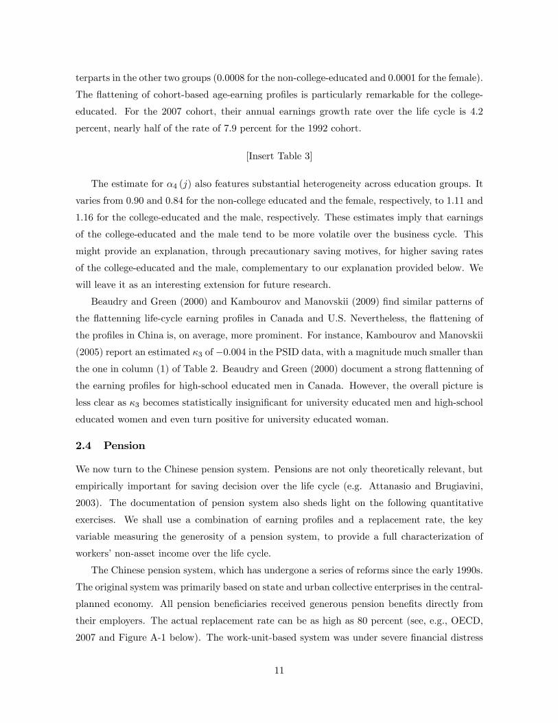
The aggregate saving rates simulated from the �rst model are plotted by solid line in Panel

A of Figure 10. Panel B displays the increase of saving rates over the life cycle from 1992 to

2007. The �tness in Panel A is impressive (Recall that the model is not calibrated to the time

path of aggregate saving rate). The simulated increase of aggregate saving rate tracks the data

closely. Quantitatively, the simulated aggregate saving rate increases by 11 percentage points

over the 16 years, identical to the increase in the data.

[Insert Figure 10]

The increase of saving rates over the life cycle (Panel B) also replicates reasonably well the

U-shaped pattern in the data. In particular, the match for the increase of saving rate for age

above 50 is improved substantially. Under myopic expectation, a fall of the replacement rate is

considered an unanticipated change to future pension bene�ts and, thus, increase further the

saving rates. Such an e¤ect grows stronger for individuals closer to the age of retirement.

The impact of social security on savings has been extensively investigated in the literature

pioneered by Feldstein (1974).20 Although our work has a focus on how changes in age earnings

pro�les a¤ect saving decision, the above quantitative exercise con�rms a large e¤ect of social

security on saving rate. The declining replacement rates alone can increase aggregate saving

rate and saving rate of the old (with age 50-60) by about 6 and 10 percentage points, respec-

tively. Moreover, a time-invariant replacement rate implies that the increase of saving rate

would monotonically decrease over the life cycle. That is to say, under myopic expectation,

the fall of replacement rate is not only quantitatively important for generating large increase

of aggregate saving rate, but also qualitatively important for a U-shaped increase of saving

rate over life cycle.

We then allow within-cohort heterogeneity by introduce di¤erent education endowments

at birth, with recalibrated �i. The dashed lines in Figure 10 plot the simulation results. The

basic features carry over to the second model.

20Using models calibrated to the U.S. economy, the literature has repeatedly illustrated a quantitatively largee¤ect of social security on household savings and, hence, interest rates in general equilibrium (e.g., amongmany others, Imrohoroglu et al., 1995; Conesa and Krueger, 1999). Empirical evidence is, however, limited andsometimes mixed. For instance, the evidence is mixed for cross-country data (Samwick, 2000). Using Italianhousehold data, Attanasio and Brugiavini (2003) �nd that a reduction of pension wealth increases saving ratessigni�cantly.

26

Finally, we check the parameter sensitivity. As before, we use the second model as the

benchmark and perturb one of the two parameters, aTr1 =wTr1 and �, in each experiment. Similar

to these experiments conducted under perfect foresight, we increase aTr1 =wTr1 from 4 to 5 in

the �rst experiment. The second experiment sets � = 0:75. The results are essentially the

same as in Figure 10, implying that the above �ndings are very robust to these alternative

parameterizations.

4.3 Family Structure and Gender Issues (Incomplete)

Demographics of family structure are potentially important for household saving decision.

Due to the one-child policy, China is undergoing a demographic transition. The average young

dependency ratio declined from 0.39 in 1992 to 0.24 in 2007, while the average old dependency

ratio rose from 0.07 to 0.10 (see Table A-1, to be added). Therefore, it is natural to check

whether the following two features are primarily driven by demographic factors: (i) the increase

of the Chinese household saving rate at the aggregate level and (ii) the U-shaped increase of the

saving rate over the life cycle. Let the saving rate for a household be the dependent variable,

and let young and old dependency ratios of the household be the regressors. Household income,

household head age and its square are also included as additional controls. We then run the

regression repeatedly for data in each UHS. The results are presented in Table A-3 (to be

added). The coe¢ cients of interests on the young and old dependency ratios are statistically

signi�cant and have the expected signs in most years. Qualitatively, these results suggest that

the declining young dependency ratios and the rising old dependency ratios contribute to the

increase of the aggregate household saving rate. Such e¤ects, however, are quantitatively not

important. For instance, the average estimated coe¢ cient on the young dependency ratio is

about -4%. Multiplied by the drop of the young dependency ratio of 0.15 from 1992 to 2007,

the estimate implies only 0.6 percentage-point increase of the aggregate saving rate over this

period. To see this more explicitly, the dotted line in Panel A of Figure 12 (to be added) plots

the dependency-ratio adjusted saving rates feature essentially the same upward trend at the

aggregate level. The di¤erence between adjusted and unadjusted aggregate saving rates is less

than one percentage point in most years. These results are in line with Chamon and Prasad

(2009), who also �nd a limited role of demographics in the rise of the aggregate household

saving rates in China.

[Insert Figure 12]

Next, we check the demographic e¤ect on life-cycle saving pro�les. The estimated e¤ects of

the old dependency ratio on household saving rate change signi�cantly from the early 1990s to

27

the later periods (see, again, Table A-1, to be added). Moreover, households with household

head age above 50 have a much higher old dependency ratio than the other households. A

combination of these two �ndings can potentially explain the recent rise of the old household

saving rate. The dotted line in Panel B of Figure 12 plots the dependency-ratio adjusted

life-cycle saving pro�le over the period 2005-2007. As expected, the demographic e¤ects turn

signi�cant for age above 50. Despite this, the demographic e¤ect per se is not strong enough

for explaining a signi�cant part of the increase of the old household saving rate. The di¤erence

between adjusted and unadjusted saving rates never exceeds two percentage points.21

We will also discuss how to deal with gender issues in the quantitative analysis.

5 Concluding Remarks

The life cycle and permanent income hypotheses represent a simple and elegant paradigm

that can be used to understand the determinants of consumption and saving decisions. While

the theory has succeeded in unifying a wide range of diverse phenomena, it is di¢ cult to

reconcile with the positive relationship between saving and income growth found in fast growing

economies or cross-country regression analysis. The puzzle is that forward-looking consumers

with standard utility should save less, not more, in anticipation of higher future income, holding

the shape of age-earnings pro�les �xed.

This puzzle is resolved in the context of the fast growing economy of China. Using a

unique national household survey covering the period 1992-2007, instead of observing stable

age-earnings pro�les as assumed either explicitly or implicitly in past studies, we found that

rapid income growth in China has dramatically raised the earnings of successive cohorts of

young workers relative to older workers. We also found that the cohort-speci�c age-earnings

pro�les have become �attened over time. Our quantitative analysis showed that an otherwise

standard life-cycle model can account well for the recent surge in household saving as well as

the U-shaped increase in saving rates over the life cycle, once we incorporated the changes in

earnings pro�les and a social security scheme of transferring pension incomes from rich and

well-educated households to poor and less-educated households during China�s transition. Our

analysis showed how income growth manifests itself in the changes in earnings pro�les over the

life cycle, suggesting a new channel for growth to a¤ect saving.

Rising saving rate is a widely observed phenomenon in fast growing economies, including the

21Alternatively, we may regress saving rate on dummies re�ecting family structure. Speci�cally, we mayinclude three dummies, for households with children only, with retirees only, with both children and retirees,respectively. This approach gives quantitatively similar results, according to our very preliminary �ndings.

28

newly industrialized countries in Eat Asia and more recently the BRICs. It remains a challenge

to validate whether the life-cycle mechanisms proposed in this paper could well explain the

rise in saving in other rapidly growing economies.

References

[1] Auerbach, Alan J. and Laurence J. Koltiko¤ (1987) �Dynamic Fiscal Policy,�Cambridge

University Press, Cambridge.

[2] Attanasio, Orazio P. and Agar Brugiavini (2003) �Social Security and Households�Sav-

ings,�Quarterly Journal of Economics, 118(3), 1075-1120.

[3] Beaudry, Paul and David A. Green (2000) �Cohort Patterns in Canadian Earnings: As-

sessing the Role of Skill Premia in Inequality Trends,�Canadian Journal of Economics,

33(4), 907-936.

[4] Carroll, Christopher D. (1994), �How Does Future Income A¤ect Current Consumption?�

Quarterly Journal of Economics, 109(1), 111-147.

[5] Carroll, Christopher D., Jody Overland and David N. Weil (2000) �Saving and Growth

with Habit Formation,�American Economic Review, 90(3), 341-355.

[6] Carroll, Christopher D. and Lawrence H. Summers (1991) �Consumption Growth Parallels

Income Growth: Some New Evidence,�National Saving and Economic Performance, eds.

B.D. Bernheim and J.B. Shoven, Chicago: Chicago University Press.

[7] Chamon, Marcos and Eswar Prasad (2009) �Why Are Saving Rates of Urban Households

in China Rising?�American Economic Journal (Macroeconomics), forthcoming.

[8] Chen, Kaiji, Ayse ·Imrohoro¼glu and Selahattin ·Imrohoro¼glu (2006) �The Japanese Saving

Rate,�American Economic Review, 96(5), 1850-1858.

[9] Conesa, Juan C. and Dirk Krueger (1999) �Social Security Reform with Heterogeneous

Agents,�Review of Economic Dynamics, 2, 757-795.

[10] Davies, James and John Whalley (1991) �Taxes and Capital Formation: How Important

is Human Capital?� National Saving and Economic Performance, B. Bernheim and J.

Shoven (eds.), University of Chicago Press, Chicago, 1991.

[11] Deaton, Angus (1991) "Saving and Liquidity Constraints." Econometrica, 59(5): 1221-48.

29

[12] Deaton, Angus and Christina H. Paxson (1994) �Saving, growth and aging in Taiwan,�

In D. Wise, ed., Studies in the Economics of Aging, University of Chicago Press, Chicago,

IL.

[13] Deaton, Angus and Christina H. Paxson (2000) �Growth and Saving Among Individuals

and Households,�Review of Economics and Statistics, 82(2), 212-25.

[14] Dunaway, Steven and Vivek Arora (2007) �Pension Reform in China: The Need for a New

Approach,�IMF Working Paper 07/109.

[15] Heckman, James J., Lance J. Lochner, and Petra E. Todd (2006) �Fifty Years of Mincer

Earnings Regressions,�Handbook of Education Economics, Vol. 1, Hanushek, E. and F.

Welch (eds.), The Netherlands: Elsevier.

[16] Feldstein, Martin S. (1974) �Social Security, Induced Retirement and Aggregate Capital

Accumulation,�Journal of Political Economy, 82(5), 905-926.

[17] Guvenen, Fatih (2007) �Learning Your Earning: Are Labor Income Shocks Really Very

Persistent?�American Economic Review, 97(3), 687-712.

[18] Imrohoroglu, Ayse, Selahattin Imrohoroglu and Douglas H. Joines (1995) �A Life Cycle

Analysis of Social Security,�Economic Theory, 6, 83-114.

[19] Kambourov, Gueorgui and Iourii Manovskii (2005) �Accounting for the Changing Life-

Cycle Pro�le of Earnings,�mimeo.

[20] Li, Zhigang and Mingqin Wu (2010) "Who Has Financed the Employer-Provided Pension

in China? A Triple-Track story." Working Paper, University of Hong Kong.

[21] Lin, Dong-hai and Yu Ding (2007) �Social Security Pension New Deal: Assessing the

Replacement Rate between Old and New,�Population & Economics, 2007(1), 70-74 (in

Chinese).

[22] Loayza, Norman, Klaus Schmidt-Hebbel and Luis Serven (2000) �What Drives Private

Saving Across the World?�Review of Economics and Statistics, 82(2), 165-181.

[23] Modigliani, Franco (1970) �The Life Cycle Hypothesis of Saving and Intercountry Di¤er-

ences in the Saving Ratio,� in Induction, Growth and Trade, eds. W. A. Eltis, M. FG.

Scott, and J. N. Wolfe, Oxford: Clarendon Press, 197-225

30

[24] Modigliani, Franco (1986) �Life Cycle, Individual Thrift, and the Wealth of Nations,�

American Economic Review, 76(3), 297-313,

[25] Modigliani, Franco and Shi Larry Cao (2004) �The Chinese Saving Puzzle and the Life-

Cycle Hypothesis,�Journal of Economic Literature, 42(1), 145-170.

[26] Michaud, Pierre-Carl and Arthur van Soest (2006) �How Did the Elimination of the

Earings Test Above the Normal Retirement Age A¤ect Retirement Expectations,�mimeo,

University of Michigan.

[27] Paxson, Christina (1996) �Saving and Growth: Evidence from Micro Data,� European

Economic Review, 40(2), 255-288.

[28] Reimers, Cordelia and Marjorie Honig (1996) �Responses to Social Security by Men and

Women: Myopic and Far-Sighted Behavior,�Journal of Human Resources, 31(2), 359-382.

[29] Samwick, Andrew A. (2000) �Is Pension Reform Conducive to Higher Saving?�Review of

Economics and Statistics, 82(2), 264-272.

[30] Storesletten, Kjetil, Christopher I. Telmer and Amir Yaron (2004) �Consumption and

Risk Sharing over the Life Cycle,�Journal of Monetary Economics, 51, 609-633.

[31] Summers, Lawrence H. (1981) �Capital Taxation and Accumulation in a Life Cycle

Growth Model,�American Economic Review, 71(4), 533-544.

[32] Tobin, James (1967) �Life Cycle Saving and Balanced Growth,�in Ten Economic Studies

in the Tradition of Irving Fisher, John Wiley. 231-56.

[33] Wei, Shang-jin and Xiaobo Zhang (2009) �The Competitive Saving Motive: Evidence

from Rising Sex Ratios and Saving Rates in China,�NBER Working Paper 15093.

[34] Wen, Yi (2009) �Saving and Growth under Borrowing Constraints: Explaining the �High

Saving Rate�Puzzle,�Federal Reserve Bank of St. Louis Working Paper 2009-045B.

[35] Yang, Dennis Tao, Junsen Zhang and Shaojie Zhou (2010) "Why Are Savign Rates So

High in China," Working Paper, The Chinese University of Hong Kong.

[36] Yang, Dennis Tao and Junsen Zhang (2010) "One-Child Policy and the Rise in Urban

Household Saving in China," manuscript, The Chinese University of Hong Kong.

[37] Zhao, Yaohui, and Jianguo Xu (2002) �China�s Urban Pension System: Reforms and

Problems,�Cato Journal, 21(3), 395-414.

31

Table 1 Regressions on Cohort-Based Age Earnings Profiles Dep. Variable Log of real annual earnings (1) (2) (3) (4) BG DP BG DP Full sample Full sample Cohorts with

entry year >= 1978

Cohorts with entry year >=

1978

Cohort 0.1210*** (3.94)

0.1109*** (22.11)

0.0885*** (2.79)

0.0962*** (12.74)

Cohort2 -0.0002 (-0.98)

-0.0001 (-0.90)

0.0000 (0.03)

0.0000 (1.01)

Cohort*Age -0.0011** (-2.37)

-0.0008*** (-10.25)

-0.0006 (-1.21)

-0.0006*** (-4.68)

Age 0.3080*** (9.32)

0.2979*** (41.60)

0.3151*** (8.21)

0.3225*** (25.57)

Age2 -0.0042*** (-11.55)

-0.0040*** (-16.07)

-0.0050*** (-8.66)

-0.0050*** (-10.55)

Age3 0.0000*** (12.18)

0.0000*** (12.15)

0.0000*** (8.09)

0.0000*** (7.99)

Detrended aggregate earnings

1.0351*** (12.12)

- 0.9880*** (11.17)

-

Year Dummies No Yes No Yes Obs. 576 576 376 376 Ad. R2 0.9831 0.9950 0.9903 0.9977 BG stands for the specification in Beaudry and Green (2000). DP stands for the specification using year dummies (rather than detrended aggregate earnings) plus the identification condition in Deaton and Paxson (1994). BG is applied for Column (1) and (3) and DP is applied for Column (2) and (4). Column (1) and (2) use full-sample data, while Column (3) and (4) contain cohorts with entry year >= 1978 only. t statistics are in parentheses. ***, ** and * stand for significance at 1%, 5% and 10%, respectively.

Table 2 Regressions on Cohort-Based Age Earnings Profiles by Education and Gender Dep. Variable Log of real annual earnings (1)

Non-college (2)

College (3)

Female (4)

Male Cohort 0.0968***

(2.68) 0.2044***

(4.24) 0.0522**

(2.43) 0.1425***

(3.88) Cohort2 -0.0002

(-0.82) -0.0009**

(-2.46) 0.0003 (0.81)

-0.0003 (1.23)

Cohort*Age -0.0008 (-1.44)

-0.0019*** (-2.68)

-0.0001 (-0.11)

-0.0014*** (-2.59)

Age 0.2116*** (5.45)

0.3271*** (6.31)

0.1956*** (4.05)

0.3911*** (9.91)

Age2 -0.0024*** (-5.71)

-0.0033*** (-5.79)

-0.0029*** (-4.15)

-0.0054*** (-12.46)

Age3 0.0000*** (5.45)

0.0000*** (4.78)

0.0000*** (4.17)

0.0000*** (12.09)

Detrended aggregate earnings

0.8973*** (8.94)

1.1055*** (8.24)

0.8443*** (6.73)

1.1611*** (11.37)

Obs. 576 576 496 576 Ad. R2 0.9687 0.9709 0.9637 0.9769 We use the specification in Beaudry and Green (2000). Column (1) to (4) use subsamples of workers who are non-college graduate (1), college graduate (2), female (3) or male (4). t statistics are in parentheses. ***, ** and * stand for significance at 1%, 5% and 10%, respectively.

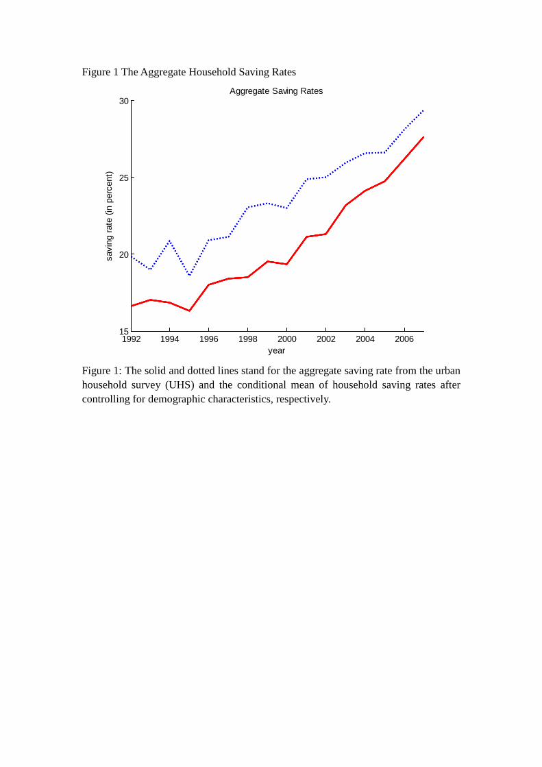
Figure 1 The Aggregate Household Saving Rates

1992 1994 1996 1998 2000 2002 2004 200615

20

25

30

year

savi

ng ra

te (i

n pe

rcen

t)

Aggregate Saving Rates

Figure 1: The solid and dotted lines stand for the aggregate saving rate from the urban household survey (UHS) and the conditional mean of household saving rates after controlling for demographic characteristics, respectively.

Figure 2 Cross-Sectional Age Saving Rate Profiles

25 30 35 40 45 50 5510

15

20

25

30

35

40

age

savi

ng ra

te (p

erce

nt)

Panel A: Average Saving Rates by Age of Household Head

1992-19932006-2007

25 30 35 40 45 50 555

10

15Panel B: Increase of Saving Rates by Age of Household Head

age

incr

ease

of s

avin

g ra

te

Figure 2: The dotted and solid lines in Panel A refer to the cross-sectional age saving rate profiles averaged over 1992-1993 and 2006-2007 (weighted by the number of observations in each age cell), respectively. The line in Panel B plots the increase of average saving rates from 1992-1993 to 2006-2007 (namely, the difference between the two profiles in Panel A). Three-age moving average is used to smooth the age saving rate profiles.

Figure 3 Cross-Sectional Age Saving Rate Profiles by Education and Gender

30 40 5010

15

20

25

30

35

40

age

savi

ng ra

te (p

erce

nt)

Panel A: Non-College Graduates

1992-19932006-2007

30 40 5010

15

20

25

30

35

40

agesa

ving

rate

(per

cent

)

Panel B: College Graduates

1992-19932006-2007

30 40 5010

15

20

25

30

35

40

age

savi

ng ra

te (p

erce

nt)

Panel C: Female

1992-19932006-2007

30 40 5010

15

20

25

30

35

40

age

savi

ng ra

te (p

erce

nt)

Panel D: Male

1992-19932006-2007

Figure 3: The dotted and solid lines refer to the cross-sectional age saving rate profiles averaged over 1992-1993 and 2006-2007 (weighted by the number of observations in each age cell), respectively. Three-age moving average is used to smooth the age saving rate profiles. Panel A to D plot the age saving rate profile for households with household head who is non-college graduate (Panel A), college graduate (Panel B), female (Panel C) or male (Panel D).

Figure 4 Cross-Sectional Life-Cycle Earnings Profiles

25 30 35 40 45 50 55-0.4

-0.3

-0.2

-0.1

0

0.1

0.2

age

log

rela

tive

earn

ings

19922007

Figure 4: The dotted and solid lines refer to the cross-sectional age earnings profiles in 1992 and 2007, respectively. Relative earnings are computed as the ratio of earnings to earnings at age 42.

Figure 5 Cross-Sectional Life-Cycle Earnings Profiles by Education and Gender

30 40 50-0.4

-0.3

-0.2

-0.1

0

0.1

0.2

age

log

rela

tive

earn

ings

Panel A: Non-College Graduates

19922007

30 40 50-0.4

-0.3

-0.2

-0.1

0

0.1

0.2

age

log

rela

tive

earn

ings

Panel B: College Graduates

19922007

30 40 50-0.4

-0.3

-0.2

-0.1

0

0.1

0.2

age

log

rela

tive

earn

ings

Panel C: Female

19922007

30 40 50-0.4

-0.3

-0.2

-0.1

0

0.1

0.2

age

log

rela

tive

earn

ings

Panel D: Male

19922007

Figure 5: The dotted and solid lines refer to the cross-sectional age earnings profiles in 1992 and 2007. Panel A to D plot the age earnings profile for households with household head who is non-college graduate (Panel A), college graduate (Panel B), female (Panel C) or male (Panel D). Relative earnings are computed as the ratio of earnings to earnings at age 42 within each group.

Figure 6 Aggregate Replacement Rates

1992 1994 1996 1998 2000 2002 2004 2006 20080.5

0.55

0.6

0.65

0.7

0.75

0.8

0.85

0.9

year

the

repl

acem

en ra

teUHSCYS

The solid line is the ratio of pensions for retired and resigned persons per capita over average wage of staff and workers. Data source: China Statistical Yearbook (2006). The dotted line is the ratio of average pensions per pension beneficiary over average earnings per worker. Data source: UHS.

Figure 7 Simulation Results under Perfect Foresight

1992 1994 1996 1998 2000 2002 2004 200615

20

25

30

year

perc

ent

Panel A: Aggregate Saving Rates

model-1model-2data

25 30 35 40 45 50 55 606

8

10

12

14

age

perc

ent

Panel B: Increase of Saving Rates by Age from 1992 to 2007

model-1model-2data

Figure 7: Solid and dashed lines are the simulated results from model-1 (no within-cohort heterogeneity) and model-2 (within-cohort heterogeneity of education levels), respectively. Panel A and B plot the increase of saving rate at the aggregate level and over the life cycle, respectively, under the benchmark parameterization (see the text for details). Dotted lines plot the increases in the data.

Figure 8 The Simulated Increase of Saving Rates over the Life Cycle

25 30 35 40 45 50 55 600

5

10

15

20

age

perc

ent

Panel A: Non-College

modeldata

25 30 35 40 45 50 55 600

5

10

15

20

age

perc

ent

Panel B: College

modeldata

Figure 8: Solid lines the simulated results from the extended model containing within-cohort heterogeneity of education levels, under the benchmark parameterization (see the text for details). Panel A and B plot the increase of saving rate for non-college and college graduates, respectively. Dotted lines plot the increases in the data.

Figure 9 Robustness Check under Perfect Foresight

1992 1994 1996 1998 2000 2002 2004 200615

20

25

30

year

perc

ent

Panel A: Aggregate Saving Rates

25 30 35 40 45 50 55 609

10

11

12

13

14

15

16

age

perc

ent

Panel B: Increase of Saving Rates by Age from 1992 to 2007

model-2experiment 1experiment 2experiment 3

model-2experiment 1experiment 2experiment 3

Figure 9: Panel A and B plot the sensitivity of the increase of saving rate at the aggregate level and over the life cycle, respectively. See the text for details on the three experiments.

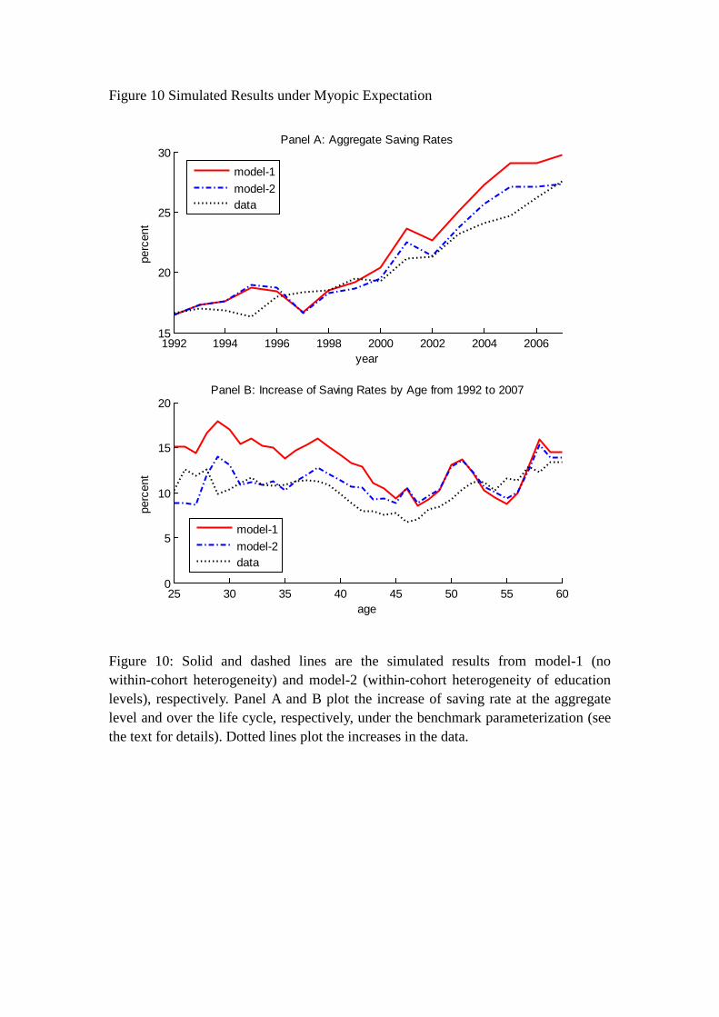
Figure 10 Simulated Results under Myopic Expectation

1992 1994 1996 1998 2000 2002 2004 200615

20

25

30

year

perc

ent

Panel A: Aggregate Saving Rates

model-1model-2data

25 30 35 40 45 50 55 600

5

10

15

20

age

perc

ent

Panel B: Increase of Saving Rates by Age from 1992 to 2007

model-1model-2data

Figure 10: Solid and dashed lines are the simulated results from model-1 (no within-cohort heterogeneity) and model-2 (within-cohort heterogeneity of education levels), respectively. Panel A and B plot the increase of saving rate at the aggregate level and over the life cycle, respectively, under the benchmark parameterization (see the text for details). Dotted lines plot the increases in the data.