Highly stable finite volume based relaxation iterative algorithm for solution of dc line ionized fields in the presence of wind

international journal of numerical modelling : electronic networks, devices and fields,Vol. 10, 355–370 (1997)

HIGHLY STABLE FINITE VOLUME BASED RELAXATIONITERATIVE ALGORITHM FOR SOLUTION OF DC LINE

IONIZED FIELDS IN THE PRESENCE OF WINDxin li, i. r. ciric and m. r. raghuveer*

Department of Electrical & Computer Engineering, The University of Manitoba, Winnipeg, Manitoba, Canada R3T 5V6

SUMMARYThis paper presents a highly stable relaxation iterative algorithm for solving the ionized fields of unipolarHVDC transmission lines in the absence or in the presence of wind. The finite element method is employedto solve Poisson’s equation, and the upwind finite volume method is applied to solve the current continuityequation. The algorithm has been tested up to a wind velocity of 45 m/s. Results obtained for a unipolarHVDC transmission line model show that the application of the upwind method increases the stability andconvergence of the iterative algorithm when wind is stronger, while the implementation of a relaxationtechnique makes it possible for the iterative algorithm to cover a wide range of wind velocities, geometricparameters and ratios of the applied voltage to the corona onset value. 1997 John Wiley & Sons, Ltd.

Int. J. Numer. Model., 10, 355–370 (1997)

No. of Figures: 21. No. of Tables: 0. No. of References: 25.

1. INTRODUCTION

Space charges created by corona discharges around the conductors of an HVDC transmission linecause environmental concerns in addition to power losses. These effects are evaluated by solvingthe electric field in the presence of space charge, i.e. the ionized field. However, the solution ofthis problem is difficult due to its nonlinearity. Additional difficulties are introduced by thepresence of wind, which may significantly influence space charge movement.

Research on the ionized field problem has been carried out for more than 80 years. Earlywork1–3 was directed towards the development of analytical solutions. In the 1960s, Sarmaet al.4

proposed a numerical solution where the problem is reduced to one dimension using Deutsch’sassumption which states that the trajectories of space charge coincide with the flux lines of thecorresponding charge-free field. Later, development in numerical solution techniques, such as thefinite difference method (FDM),5,6 the finite element method (FEM),7–13 the boundary elementmethod (BEM)14,15 and the finite volume method (FVM),16 made it possible to improve theaccuracy of the solutions by discarding Deutsch’s assumption which is not valid in the presenceof wind. In recent years, a number of solutions of the ionized field in the presence of wind havebeen developed.12–15,17–21However, in the solution techniques reported in the literature, the windvelocities considered do not exceed 12 m/s.

Recently, the authors22 developed two upwind finite volume algorithms for solving the ionizedfield in the presence of extremely strong wind. Although these algorithms perform better withincrease in wind velocity, they suffer from instability at lower wind velocities and higher ratiosof the applied voltage to the corona onset value. In this paper, a relaxation technique is proposedto overcome these drawbacks and make the solution stable for any wind velocity that can beencountered in practice. Moreover, an upwind parameter has been introduced, whose valuedetermines the weight assigned to the upwind feature in the finite volume method for solving thecurrent continuity equation. Numerical tests are carried out on a line-plane model to investigatethe influence of different factors on the iterative behaviour. The ground profiles of electric field

*Correspondence to: M. R. Raghuveer, Department of Electrical and Computer Engineering, The University ofManitoba, Winnipeg, Manitoba, Canada R3T 5V6

CCC 0894–3370/97/060355–16$17.50 Received 25 March 1997 1997 John Wiley & Sons, Ltd. Revised 28 July 1997

356 x. li, i. r. ciric and m. r. raghuveer

strength and space charge density obtained by the present method are compared with thoseobtained by other methods12,13,15 and with the measured values.23

2. MODELLING OF UNIPOLAR IONIZED FIELD

The ionized field of an HVDC transmission line is usually modelled as a two-dimensional, time-independent field, described by

=2u = −r/ε0 (1)

= · (rv) = 0 (2)

where u is the electric potential,r the space charge density,ε0 the permittivity of free space andv the space charge drift velocity, which is determined, when the line is positively energized, by

v = − k=u + w (3)

where k is the ionic mobility andw the wind velocity.Equation (1) is Poisson’s equation and equation (2) the current continuity equation. The solution

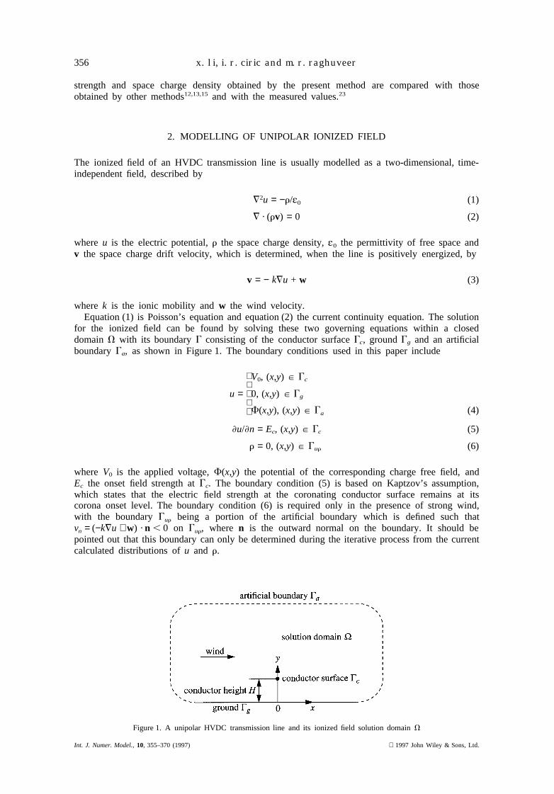
for the ionized field can be found by solving these two governing equations within a closeddomainV with its boundaryG consisting of the conductor surfaceGc, groundGg and an artificialboundaryGa, as shown in Figure 1. The boundary conditions used in this paper include

V0, (x,y) P Gc

u =

0, (x,y) P Gg

F(x,y), (x,y) P Ga (4)

u/n = Ec, (x,y) P Gc (5)

r = 0, (x,y) P Gur (6)

where V0 is the applied voltage,F(x,y) the potential of the corresponding charge free field, andEc the onset field strength atGc. The boundary condition (5) is based on Kaptzov’s assumption,which states that the electric field strength at the coronating conductor surface remains at itscorona onset level. The boundary condition (6) is required only in the presence of strong wind,with the boundaryGur being a portion of the artificial boundary which is defined such thatvn = (−k=u + w) · n , 0 on Gur, where n is the outward normal on the boundary. It should bepointed out that this boundary can only be determined during the iterative process from the currentcalculated distributions ofu and r.

Figure 1. A unipolar HVDC transmission line and its ionized field solution domainV

Int. J. Numer. Model.,10, 355–370 (1997) 1997 John Wiley & Sons, Ltd.

357relaxation iterative algorithm

3. ITERATIVE ALGORITHM

3.1. Preliminary considerations

The algorithm proposed in this paper is constructed by considering the electric potentialu toconsist of two components. The first component,F, is due to the applied voltage when no spacecharge is present and is the solution of the following boundary value problem:

=2F = 0

FuGc= V0

FuGg= 0 (7)

This problem can be solved either numerically or analytically in the case of a unipolar HVDCtransmission line. The other component,w, is caused by the space charge, and satisfies the Poissonequation with a homogeneous Dirichlet boundary condition,

=2w = −r/ε0 in V

wuG = 0 (8)

This boundary value problem can be uniquely solved if the charge distribution is known. Obviously,if wp is a solution for the problem corresponding torp, thenawp is a solution corresponding toarp, wherea is an arbitrary constant.

Thus the electric potentialu corresponding to a space charge density

r = arp (9)

can be written as

u = F + awp (10)

u and r in equations (9) and (10) satisfy Poisson’s equation (1) and the boundary condition (4)for any constanta. To also satisfy the boundary condition (5),a is determined as

a = (Ec − EFcond)/Ewcond (11)

where Ec is the corona onset field strength,EFcond the electric field strength atGc due to F, andEwcond the electric field strength atGc due to wp. The electric potential and the space chargedensity must also satisfy the current continuity equation (2). This is achieved by modifyingiteratively the charge density and the potential. The process consists in calculating a newdistribution of charge density from the current continuity equation using the potential given byequation (10). Subsequently a new distribution of potential is obtained from equation (8), whichleads to a new potential in (10) witha from (11). This is repeated until convergence is reached.

3.2. Relaxation iterative algorithm

Based on the above discussion, the relaxation iterative algorithm takes the following form:

Step 1: Solve the boundary value problem (7) to obtain the potentialF; set k = 1, u(k) = F andr(k)

cond= r(0)cond, wherer(k)

cond is the space charge density atGc and r(0)cond an initial guess for

the space charge density atGc.Step 2: Let r(k) = r(k)

cond at Gc and r(k) = 0 at Gur; obtain r(k) by solving the current continuityequation (2) based on the given distributionu(k).

Step 3: Solve the boundary value problem (8) forw(k) using r(k); calculateE(k)wcond.

1997 John Wiley & Sons, Ltd. Int. J. Numer. Model.,10, 355–370 (1997)


Step 4: Calculateak = (Ec − EFcond)/E(k)wcond; if u1 − aku , d, whered is a specified tolerance, then

terminate the iteration; otherwise proceed to step 5.Step 5: Update the potential in the entire solution domain and the charge density atGc,

respectively, as:

u(k+1) = F + akw(k) (12)

r(k+1)cond = akr

(k)cond (13)

Step 6: Perform the relaxation procedure:

u(k+1) = u(k) + u1(u(k+1) − u(k)) (14)

r(k+1)cond = r(k)

cond + u2(r(k+1)cond − r(k)

cond) (15)

In this paper, we present results foru1 = u2 = u.Step 7: Set k ⇐ k + 1 and repeat the iterative process from step 2.

The parameterak is used to update the quantities in thekth iteration, and also serves as a measureof convergence. The relaxation factoru is chosen in the range 0, u , 1. The solutions ofPoisson’s equation and the current continuity equation in steps (2) and (3) are described in thenext two Sections.

4. FEM FOR POISSON’S EQUATION

The general form of the boundary value problems (7) and (8) in steps 1 and 3, respectively, ofthe iterative algorithm is

=2c = −q in V

cuG = f0 (16)

where the potentialc is unknown,q a given function andf0 a specified distribution onG. Thefinite element method (FEM)24 is employed to solve this problem. Let the solution domainV beapproximated by a finite element mesh consisting ofne triangular elements andnp nodes. It canbe shown that the weak form of the weighted residual statement for Poisson’s equation is

EV

=Nl · =cdxdy − EV

Nlqdxdy − EVl>G

Nlgds = 0, l = 1,2,%,np (17)

with

g = c/n (18)

c = { N}{ c} (19)

where {c} = { c1,c2,%,cnp} T represents the nodal values ofc, {N} = { N1,N2,%,Nnp

} the globalshape functions, andVl the subdomain which covers the elements adjacent to nodel. In the thirdintegral of equation (17), the quantityg over Vl>G may be taken to be a constant which isdenoted bygl. Inserting the expansion forc gives

[K] { c} − { b} − [Z] { g} = {0} (20)

where [K], [b] and [Z] are defined as follows:

[K] = EVS

x{ N} T

x{ N} +

y{ N} T

y{ N}Ddxdy (21)



[b] = EV

{ N} Tqdxdy (22)

[Z] = diag [Z1,Z2,%,Znp] (23)

with

Zl = EVl>G

Nlds (24)

The vector {g} in equation (20) is defined such that its elementgi = c/nui if node i P G andgi = 0 if node i ¸ G.

In the above system of equations, the matrix [K] is symmetric and sparse, and if nodes areproperly numbered it is a banded matrix as well. The solution of the system of equations (20)subject to the specified boundary conditions can be obtained by using the LU decompositionmethod, which requires about 0·5m2

Knp multiplications, wheremK is the average half-bandwidth ofthe matrix [K]. The outward normal componentgi at node i P G can then be obtained fromequation (20), i.e.

gi =1ZiSO

j

Kijcj − biD (25)

5. FVM FOR THE CURRENT CONTINUITY EQUATION

In this Section, the solution of the current continuity equation (2) in step 2 of the iterativealgorithm, using two finite volume methods, is discussed, assuming that the electric potentialuis given.

5.1. Node-centred finite volume method

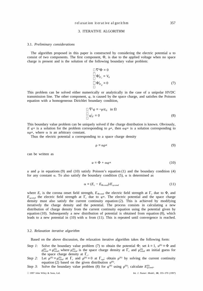
The finite volume method starts with a set of control volumes (or cells), which are constructedin the following manner. For an inner nodei, the associated control volumeCi is defined by apolygon which is formed by connecting the centres of gravity of all adjacent elements, as shownin Figure 2(a). At a boundary nodei, the construction of the cell is illustrated in Figure 2(b),where Mij and Mik are the midpoints of the sidesij and ik, respectively. Denote the common sideof cells Ci and Cj by Cij, the set of cells sharing common sides with the cellCi by IC(i), and theboundary of the cellCi by Ci. The space charge density in each cellCi is assumed to be aconstant which is denoted byri.

Applying Green’s formula, the current continuity equation (2) becomes

Figure 2. Construction of the control volume around an inner nodei or a boundary nodei



OjPI

C(i)

ECij

rijv · n ds + ECi>G

riv · n ds = 0, i = 1,2,%,np (26)

Considering the space charge densityrij to be constant along the sideCij, we have

OjPIC(i)

rijvij + rivBi = 0, i = 1,2,%,np (27)

with vij and vBi approximated by

vij = ECij

v · n ds = [k(E(1)ij + E(2)

ij )/2 + w] ·ECij

n ds (28)

vBi = ECi>G

v · n ds = −kLBigi + w · ECi>G

n ds (29)

where E(1)ij andE(2)

ij are the calculated electric field strengths at the centres of gravityG(1)

ij andG(2)ij of the two elements sharing the sideij (see Figure 3),k is the ionic mobility, LBi

the length ofCi>G, andgi the ith nodal value ofu/n, which is calculated using equation (25).In this paper, the density of space charge flowing through the common sideCij is approximated by

rij = Fri + rj

2+ gupw

ri − rj

2sign (vij)G (30)

where sign (vij) = −1 if vij , 0 and sign (vij) = 1 if vij $ 0, andgupw is an upwind parameter, whichdetermines how the space charge densityrij is influenced by the two adjacent cells. The value ofgupw is chosen in the range from 0 to 1. Whengupw = 0, rij takes the average value of the spacecharge densities of cellsCi and Cj. If 0 , gupw , 1, it implies thatrij is more influenced by thespace charge density on the upwind side. Ifgupw = 1, rij on the sideCij takes the value of thespace charge density on its upwind side, which physically means that the space charge densityof the cell Ci is only influenced by the space charge densities on its upwind side. Substitution ofequation (30) in (27) yields the system of equations

[A] { r} = {0} (31)

where [A] is an np × np matrix with its elements defined as

OsPIC(i)

12

[1 + gupwsign (vis)]vis + vBi, for the diagonal entries

Aij =

1

2[1 − gupwsign (vij)]vij, for j P IC

(i)

0, otherwise (32)

Figure 3. SideCij associated with the centres of gravity of two triangular elements



The above system of equations is solved using the Gaussian elimination method after the spacecharge densities of cells adjacent toGc < Gur are specified as indicated in step (6) of the mainiterative algorithm in Section 3. The non-symmetric sparse matrix [A] is stored in a two-dimensionalarray of dimensionsnp × 2mAm, where mAm is the maximum half-bandwidth of the matrix [A].Since a control volume is uniquely associated with a node,mAm is identically equal to themaximum half-bandwidth of the matrix [K]. The number of multiplications required for thesolution is aboutm2

Amnp. This number is about twice that for the solution of the discretizedPoisson’s equation (20) if the finite element mesh for the unipolar line model is properly numbered.Therefore, the total computational effort required for each iteration in the associated iterativealgorithm is about three times that for the solution of the discretized Poisson equation.

5.2. Triangular finite volume method

In the triangular FVM, each triangular element is taken as a cell. In addition, each boundarysegment is defined as a special type of cell, called a ‘segment cell’, which serves as the sourceor sink of stream lines. The segment cells are numbered withne + 1, ne + 2,%,ncell, where ne isthe number of elements. Following a similar discretization procedure as in the previous Section,we obtain a linear system of equations

[A] { r} = {0} (33)

where [A] is an ne × ncell matrix and its elements are defined as

OsPI

C(i)

12

[1 + gupwsign(vis)]vis, for the diagonal entries

Aij =

1

2[1 − gupwsign(vij)]vij, for j P IC

(i)

0, otherwise (34)

with

vij =

FkSSij − sij

Sij

Eoi +sij

Sij

EojD + wG ·ECij

n ds, for j # ne

−kLij(gl + gm) + w · ECij

n ds, for j . ne

(35)

where Eoi and Eoj are the calculated field strengths at the centres of gravityOi and Oj of the twocells Ci and Cj sharing the sideCij (see Figure 4),Sij the length of the segmentOiOj, sij thelength of the segmentOiQ, and gl,gm are the values ofu/n at the two terminal pointsl and mof the sideCij on the boundary which are determined from equation (25).

The resulting system of equations, whengupw = 1, can be solved in a simple way. As shown

Figure 4. SideCij shared by two cells



Figure 5. Space charge densityri in the cell Cij influenced by the cells on its upwind side: (a)ri influenced by one cell;(b) ri influenced by two cells

in Figure 5, the space charge densityri in the cell Ci is only influenced by one or two cells. Ifthe space charge densities on the upwind side of the cellCi have been evaluated, the space chargedensity ri can be easily determined as

ri = −1Aii

OjPICupw

(i)

Aijrj (36)

where ICupw(i) , IC

(i) is the set of triangular cells on the upwind side of the cellCi. It is possible toobtain all the cell space charge densities by using equation (36), starting from the cells whosesides are onGc < Gur to the cells on the downwind side once the charge densities of the segmentcells on Gc < Gur are evaluated. To do this, first we define a vector {nuw} such that nuw

i + 1represents the number of variables to be determined in theith equation of the system ofequations (33). The values of the components in {nuw} will vary as the solution process proceeds.The initial value of nuw

i is the number of triangular cells in the setICupw(i) . If the value of nuw

i

becomes zero, it indicates that only the quantityri in the ith equation is undetermined. Thecalculation scheme is described as follows:

Step 1: Generate the vector {nuw} and setm = 0.Step 2: For i = 1,2,%,ne, if nuw

i = 0, carry out the following procedure:

ri = −1

AiiO

jPICupw(i)

Aijrj

nuwi ⇐ nuw

i − 1

nuwj ⇐ nuw

j − 1 for all j P ICupw(i)

m ⇐ m + 1

Step 3: If m= ne, stop; otherwise go to step 2.

Since the average number of cells in the setICupw(i) is about 1·5, the total number of multiplications

and divisions required in the above scheme is about 2·5ne or 5np since ne . 2np for a triangularelement mesh. This number is negligibly small compared to that required by the LU decompositionmethod or the Gaussian elimination method. Thus, the solution of Poisson’s equation is responsiblefor most of the computational work for each iteration in the iterative algorithm.

6. NUMERICAL TESTS

This Section presents numerical tests of the iterative algorithm outlined in Section 3 on a line-plane model. As indicated in step 4 of Section 3.2, convergence is considered to have beenobtained whenu1 − aku , d; the toleranced is specified to be 1% in this paper. The behaviour ofthe iterative algorithm (i.e. stability of algorithm and rate of convergence) is investigated inSections 6.2 and 6.3, and is shown in Figures 7–14. These results were obtained by using the



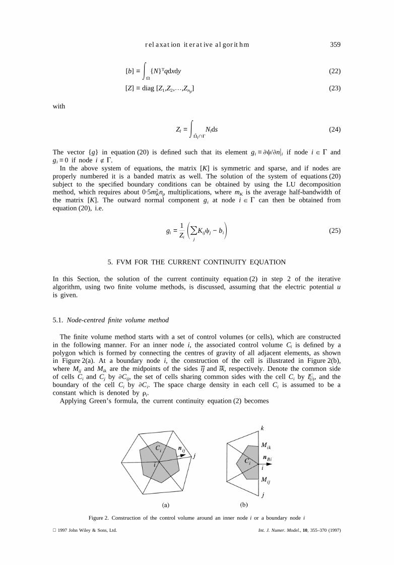
Figure 6. FE mesh for the line-plane model:ne = 2476, np = 1291, r0 = 0·0025 m,H = 2 m

method in Section 5.1 to solve the current continuity equation. It may be remarked that theiterative behaviour remains almost the same when the method in Section 5.2 is applied. Theground profiles of the field quantities presented in Figures 17–21 are calculated using both methods.

6.1. Test models

The line-plane model consists of a cylindrical conductor of radiusr0 = 0·0025 m situated at aheight H = 2 m above ground (see Figure 1). The corona onset field strength isEc = 48·06 kV/cmas obtained from Peek’s law, and the corona onset voltage isVc = 88·64 kV.

The open domain is truncated by an artificial boundary which is located 5H above and 7Hlaterally from the conductor. The triangular element mesh, as shown in Figure 6, is generated byan automatic mesh generation program.25 In the mesh, the numbers of elements and nodes arene = 2476 andnp = 1291, respectively.

The effect of the geometric parameters on the iterative behaviour is examined in two ways.First, the conductor radiusr0 is changed, thus enabling examination of the effect of the ratioH/r0

within a practical range. The effect of the conductor heightH on the iterative behaviour isexamined by increasing the heightH while keeping the ratioH/r0 constant.

6.2. Effect of relaxation

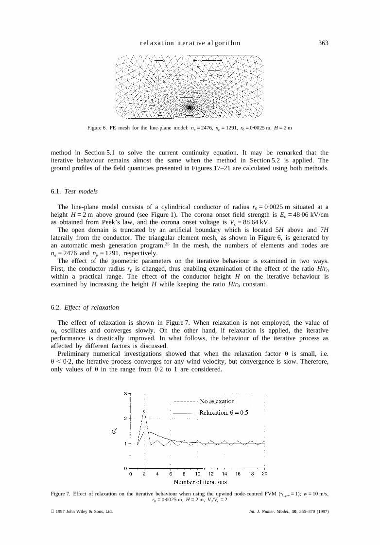
The effect of relaxation is shown in Figure 7. When relaxation is not employed, the value ofak oscillates and converges slowly. On the other hand, if relaxation is applied, the iterativeperformance is drastically improved. In what follows, the behaviour of the iterative process asaffected by different factors is discussed.

Preliminary numerical investigations showed that when the relaxation factoru is small, i.e.u , 0·2, the iterative process converges for any wind velocity, but convergence is slow. Therefore,only values ofu in the range from 0·2 to 1 are considered.

Figure 7. Effect of relaxation on the iterative behaviour when using the upwind node-centred FVM (gupw = 1); w = 10 m/s,r0 = 0·0025 m,H = 2 m, V0/Vc = 2



Figure 8. Effect of the relaxation factoru on the number of iterations required for convergence when using the upwindnode-centred FVM (gupw = 1) for different wind velocities;r0 = 0·0025 m,H = 2 m, V0/Vc = 2

Figure 8 shows the dependence of the number of iterations,niter, required on the relaxationfactor u for different wind velocities. It is seen that for each curve,u has an optimum value atwhich niter reaches its minimum. This optimum point shifts to the right for a larger wind velocityand the corresponding minimum ofniter becomes smaller. To the left of the optimum point,niter

increases slowly asu is decreased, but on the right,niter increases drastically with increase inu.In the case of still air, whenu . 0·6, convergence cannot be obtained. The usable range ofubecomes larger as the wind velocity increases. For very strong wind, the iterative process isconvergent for anyu between 0·2 and 1·0. It is interesting to note that, foru = 1, convergencecan only be obtained for very strong wind.

Since the performance of the present iterative algorithm is better in wind conditions than instill air, further numerical investigations in this Section are carried out only under no windconditions. Figure 9 illustrates the influence of the voltage ratioV0/Vc on niter. As the voltage ratioV0/Vc is increased, the optimum value ofu decreases and the usable range ofu becomes smaller.

Figure 10 shows that the number of iterations for convergence is almost unaffected by the ratioH/r0, and Figure 11 indicates that the conductor heightH practically has no effect on the iterativebehaviour for a constant value of the ratioH/r0.

From the above numerical results, it can be concluded thatu should be chosen in the range0·2 to 0·5 for light wind, and larger than 0·5 for strong wind. In the case of a very large ratioV0/Vc (e.g. .4) and light wind,u should be chosen in the range 0·2 to 0·4.

6.3. Upwind effect

Figure 12 clearly shows the effectiveness of the upwind algorithm. The necessity of using theupwind algorithm when wind is present can be seen by comparing the results in Figure 13 withthose in Figure 8. Whengupw = 0, as shown in Figure 13, as the wind velocity increases, the

Figure 9. Effect of the relaxation factoru on the number of iterations required for convergence when using the upwindnode-centred FVM (gupw = 1) for different values ofV0/Vc; w = 0 m/s, r0 = 0·0025 m,H = 2 m



Figure 10. Effect of the relaxation factoru on the number of iterations required for convergence when using the upwindnode-centred FVM (gupw = 1) for different values ofH/r0; H = 2 m, w = 0 m/s, V0/Vc = 2

Figure 11. Effect of the relaxation factoru on the number of iterations required for convergence when using the upwindnode-centred FVM (gupw = 1) for different values ofH;H/r0 = 800, w = 0 m/s, V0/Vc = 2, np = 1291

Figure 12. Effect of using the upwind node-centred FVM on the iterative behaviour in the absence of wind;u = 0·5,r0 = 0·0025 m,H = 2 m, V0/Vc = 2

usable range ofu becomes smaller and eventually relaxation cannot be used to make the iterativeprocess converge; but the opposite is true for the upwind algorithm (see Figure 8).

Figure 14 illustrates the influence ofgupw in the range from 0 to 1·0 on the required numberof iterations at different wind velocities. An interesting fact is observed from this Figure, i.e. thevariation of gupw in the range indicated has almost no effect on the convergence rate both in stillair and in wind conditions. Also, the effect ofgupw on the calculated results is very small, asshown in Figures 15 and 16.



Figure 13. Effect of wind velocity on theniter–u curve whengupw = 0; r0 = 0·0025 m,H = 2 m, V0/Vc = 2

Figure 14. Effect of the upwind parametergupw on the number of iterations required for convergence with the node-centredFVM for different wind velocities;r0 = 0·0025 m,H = 2 m, V0/Vc = 2

6.4. Ground profiles of the field quantities

Figures 17 and 18 compare the ground profiles of electric field strength and space chargedensity, respectively, in the absence of wind, obtained by the present methods and the FEM12,13

using the same finite element mesh. The results calculated using the presented two FVMs showexcellent agreement with those obtained using the FEM.12,13

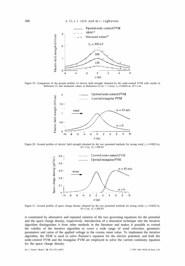
Also, the ground profiles of electric field strength determined by the presented node-centredFVM show good agreement with those obtained by the BEM,15 and compare favourably with themeasured values, as shown in Figure 19.

Figure 15. Calculated ground profiles of electric field strength obtained by using the node-centred FVM in the absence ofwind; r0 = 0·0025 m,H = 2 m, V0/Vc = 2



Figure 16. Calculated ground profiles of space charge density obtained by using the node-centred FVM in the absence ofwind; r0 = 0·0025 m,H = 2 m, V0/Vc = 2

Figure 17. Comparison of the ground profiles of electric field strength obtained by different methods in the absence ofwind; r0 = 0·0025 m,H = 2 m

Figure 18. Comparison of the ground profiles of space charge density obtained by different methods in the absence ofwind; r0 = 0·0025 m,H = 2 m

The change in the ground profiles of electric field strength and space charge density due tostrong wind is shown in Figures 20 and 21, respectively. The results using the two presentedFVMs agree satisfactorily. For this group of results, no published data are available for comparison.

7. CONCLUSIONS

A highly stable iterative algorithm has been proposed for the numerical solution of the ionizedfield of HVDC transmission lines. The framework for the construction of the iterative algorithm



Figure 19. Comparison of the ground profiles of electric field strength obtained by the node-centred FVM with results inReference 15 and measured values in Reference 23 (w , 1 m/s); r0 = 0·0025 m,H = 2 m

Figure 20. Ground profiles of electric field strength obtained by the two presented methods for strong wind;r0 = 0·0025 m,H = 2 m, V0 = 200 kV

Figure 21. Ground profiles of space charge density obtained by the two presented methods for strong wind;r0 = 0·0025 m,H = 2 m, V0 = 200 kV

is constituted by alternative and repeated solution of the two governing equations for the potentialand the space charge density, respectively. Introduction of a relaxation technique into the iterativealgorithm distinguishes it from other methods in the literature and makes it possible to extendthe validity of the iterative algorithm to cover a wide range of wind velocities, geometricparameters and ratios of the applied voltage to the corona onset value. To implement the iterativealgorithm, the FEM is used to solve Poisson’s equation for the electric potential, and both thenode-centred FVM and the triangular FVM are employed to solve the current continuity equationfor the space charge density.



Application of the triangular FVM allows solution of the resulting system of equations by usinga simple method which needs negligible computational work. As a result, the computational effortfor the corresponding iterative algorithm is about one-third of that when the node-centred FVMis used.

From numerical tests conducted on a line-plane model, the following conclusions may be drawn:

1 The geometric parameters, i.e. the ratioH/r0 and the conductor heightH, have almost no effecton the iterative behaviour for a fixed voltage ratioV0/Vc. This implies that the numerical resultspresented in this paper are quite general in a practical sense.

2 In strong wind conditions, the upwind scheme is necessarily required. Even in the case of lightwind, the upwind algorithm performs better than in the case whengupw = 0. The iterativebehaviour is almost unaffected bygupw, as long as it is larger than a small number (e.g..0·1).In addition, gupw has a negligible effect on the calculated ground profiles of the field quantities.

3 The upwind scheme yields excellent results in the presence of strong wind. In fact, the strongerthe wind, the faster and more stable the associated iterative process.

4 Introduction of the relaxation technique into the iterative algorithm is crucial to ensure itsstability and fast convergence in all situations. As for the choice of the relaxation factoru, itis recommended thatu be chosen in the range 0·2, u # 0·5 for light wind, and 0·5, u # 0·1for strong wind. For a very high ratioV0/Vc (e.g. .4) with light wind, u should be between0·2 and 0·4.

5 The ground profiles of the field quantities, in the case of still air, obtained by the presentFVMs, agree well with those obtained by other numerical methods12,13,15 and also showsatisfactory agreement with the available measured values.23

6 The ground profiles calculated using the two presented FVMs compare favourably for a windvelocity up to 45 m/s. It should be mentioned that the iterative algorithms presented remainstable even at higher wind velocities.

ACKNOWLEDGEMENTS

Financial support from the Natural Sciences and Engineering Research Council of Canada (NSERC)and Manitoba Hydro is gratefully acknowledged.

REFERENCES

1. J. S. Townsend, ‘The potentials required to maintain currents between coaxial cylinders’,Phil. Mag., 28, 83–90 (1914).2. W. Deutsch, ‘U¨ ber Die Dichtverteilung Unipolarer Ionenstro¨me’, Annalen der Physik, 5, 589–613 (1933).3. V. I. Popkov, ‘On the theory of unipolar DC corona’,Elektrichestvo, (1), 33–48 (1949),Technical Translation 1093,

National Research Council of Canada.4. M. P. Sarma and W. Janischewskyj, ‘Analysis of corona losses on DC transmission lines: I–Unipolar lines’,IEEE

Trans., PAS-88, 718–731 (1969).5. J. R. McDonald, W. B. Smith, H. W. Spencer III and L. E. Sparks, ‘A mathematical model for calculating electrical

conditions in wire-duct electrostatic precipitation devices’,J. Appl. Phys., 48, 2231–2243 (1977).6. P. A. Lawless and L. E. Sparks, ‘A mathematical model for calculating effects of back corona in wire-duct electrostatic

precipitators’,J. Appl. Phys., 51, 242–256 (1980).7. W. Janischewskyj and G. Gela, ‘Finite element solution for electric fields of coronating DC transmission lines’,IEEE

Trans., PAS-98, 1000–1012 (1979).8. T. Takuma, T. Ikeda and T. Kawamoto, ‘Calculations of ion flow fields of HVDC transmission lines by the finite

element method’,IEEE Trans., PAS-100, 4082–4810 (1981).9. M. Abdel-Salam, M. Farghally and S. Abdel-Sattar, ‘Finite element solution of monopolar corona equation’,IEEE

Trans., EI-18, 110–119 (1983).10. J. L. Davis and J. F. Hoburg, ‘Wire-duct precipitator field and charge computation using finite element and

characteristics methods’,J. Electrostat., 14, 187–199 (1983).11. Xin Li, M. R. Raghuveer and I. M. R. Ciric, ‘A new method for solving ionized fields associated with HVDC

transmission lines’,Conference on Electrical Insulation and Dielectric Phenomena (CEIDP), Virginia Beach, Virginia,USA, 22–25 October 1995.

12. Xin Li, I. R. Ciric and M. R. Raghuveer, ‘A new method for solving ionized fields of unipolar HVDC lines includingeffect of wind. Part I: FEM formulation’,Int. J. Numer. Model., Electron. Netw. Devices Fields, 10, 47–56 (1997).

13. Xin Li, M. R. Raghuveer and I. R. Ciric, ‘A new method for solving ionized fields of unipolar HVDC lines includingeffect of wind. Part II. Iterative techniques and numerical tests’,Int. J. Numer. Model., Electron. Netw. Devices Fields,10, 57–69 (1997).

14. Ming Yu and E. Kuffel, ‘A new algorithm for evaluating the fields associated with HVDC power transmission linesin the presence of corona and strong wind’,IEEE Trans., MAG-20, 1985–1988 (1993).

15. Ming Yu, The Study of Ionized Fields Associated with HVDC Transmission Lines in the Presence of Wind, Ph.Ddissertation, Department of Electrical & Computer Engineering, University of Manitoba, 1993.

16. P. L. Levin and J. F. Hoburg, ‘Donor cell-finite element descriptions of wire-duct precipitator fields, charges, andefficiencies’, IEEE Trans., IA-26, 662–670 (1990).

17. S. Abdel-Sattar, ‘Numerical method to calculate corona profiles at ground level and underneath monopolar lines asinfluenced by wind’,IEEE Trans., EI-21, 205–211 (1986).



18. T. Takuma and T. Kawamoto, ‘A very stable calculation method for ion flow field of HVDC transmission lines’,IEEE Trans., PWRD-2, 189–198 (1987).

19. B. L. Qin, J. N. Sheng, Z. Yan and G. Gela, ‘Accurate calculation of ion flow field under HVDC bipolar transmissionlines’, IEEE Trans., PWRD-3, 368–376 (1988).

20. J. Poltz and E. Kuffel, ‘A new method for the two-dimensional bipolar ion flow calculation’,6th InternationalSymposium on High Voltage Engineering, New Orleans, LA, U.S.A., 28 August–1 September 1989.

21. Y. Sunaga, Y. Amano and T. Suda, ‘Method for calculating ion flow field around an HVDC line in the presenceof wind’, 6th International Symposium on High Voltage Engineering, New Orleans, LA, U.S.A., 28 August–1September 1989.

22. Xin Li, M. R. Raghuveer and Ciric, ‘Recent advances in numerical solution of ionized fields associated with unipolarHVDC transmission lines in the presence of wind’,10th International Symposium on High Voltage Engineering,Montreal, Quebec, Canada, 25–29 August 1997.

23. M. Hara, N. Hayashi, K. Shiotsuki and M. Akazaki, ‘Influence of wind and conductor potential on distributions ofelectric field and ion current density at ground level in DC high voltage line to plane geometry’,IEEE Trans., PAS-101, 803–814 (1982).

24. O. C. Zienkiewicz and K. Morgan,Finite Elements and Approximation, J Wiley, 1983.25. Xin Li, ‘An automatic triangular mesh generation scheme for arbitrary planar domains’,Trans. Chinese Electrotechnical

Society, (4), 41–45 (1991).

Authors’ biographies:

Xin Li received his B.Sc. and M.Sc. degrees in electrical engineering from the HarbinInstitute of Electrical Technology, Harbin, China, in 1982 and 1984, respectively. Hisresearch interests include HV insulation techniques, numerical analysis of electromagneticfields and user-friendly FEM software. He is currently working towards a Ph.D. degreein the Department of Electrical and Computer Engineering at the University of Manitoba,Winnipeg, Canada. His Ph.D research topic is in the study of ionized fields.

I. R. Ciric is a professor of electrical engineering at the University of Manitoba,Winnipeg, Canada. His major interests are in the mathematical modelling of stationaryand quasistationary fields, electromagnetic fields in the presence of moving solid conduc-tors and levitation, field theory of special electrical machines, DC corona ionized fields,analytical and numerical methods for wave scattering problems, propagation alongwaveguides with discontinuities, transients and inverse problems. He has published over160 technical papers and three electrical engineering textbooks, and has been a contributorto chapters on magnetic field modelling and electromagnetic scattering by complexobjects for three books. Dr. Ciric is a Fellow of the IEEE and a member of theElectromagnetics Academy. He is listed in Who’s Who in Electromagnetics.

M. R. Raghuveer obtained his B.Sc.(Hons.), B.E. and Ph.D. degrees in 1960, 1963 and1972, respectively. He is currently a professor in the Department of Electrical andComputer Engineering at the University of Manitoba, Winnipeg, Canada. His researchinterests lie in the areas of modelling/simulation, power apparatus, device/high voltage(HV) phenomena, and applied experimental research in H.V. insulation including diagnos-tic test techniques. He is the author/coauthor of over 60 publications including anelectrical engineering textbook.


Documents

Highly stable finite volume based relaxation iterative algorithm for solution of dc line ionized fields in the presence of wind