HIGHWAY PROGRAMING, INFORMATION MANAGEMENT …

i

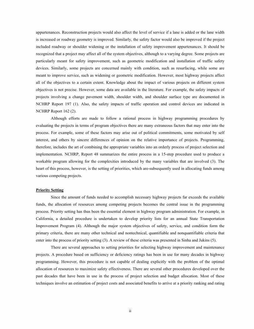
HIGHWAY PROGRAMING, INFORMATION MANAGEMENT EVALUATION METHODS

Kumares C. Sinha, Purdue University

Cf. Enhancing Highway Safety Through Engineering Management,

Transportation Research Board, Final Report of a Conference, Nov 2-5, 1981, St. Louis, Missouri

INTRODUCTION

Highway safety continues to be a major issue in the transportation area. Although significant progress

has been made in improving highway safety during the past decade, recent developments in the highway

transportation sector pose a serious problem to highway safety. While the highway system in this country is

aging and the composition of the traffic stream is changing with smaller cars and larger trucks, the need for

highway maintenance and safety improvement becomes even more important. However, the financial resources

available for the maintenance and improvement of highway facilities are declining. In an era of limited

resources, it is imperative that much care be taken in allocating funds among various highway activities related

to construction, maintenance, and operation to entire optimal cost effectiveness. Highway programming and

administration must explicitly consider safety effectiveness along with other objectives such service, condition,

and external factors, including energy and environment. A management approach is necessary to identify those

engineering elements at would best enhance highway safety within the constraints of budget and at the same time

satisfy service needs, preserve the physical condition of the facilities, and fulfill the national goals of energy and

environment.

HIGHWAY PROGRAMMING

Highway programming involves a process of selecting and scheduling improvement projects on the

basis of the relative urgency of the work. A key element of process is the matching of needed projects with

available funds to accomplish the highway improvement objectives during a given period.

System Objectives

Highway improvement objectives can generally be grouped into four major categories: safety, service,

condition, and energy and environment. Reduction of potential accidents is a primary concern in highway design

and maintenance. As the function of a highway system is to provide service to the public, improvement of the

level of service is also an important objective. At the same time, consideration must be given to protect the

capital investment already made in highway facilities, and thus the preservation of the physical condition

becomes another important objective. The next major objective of highway activities involves externalities,

particularly associated with energy conservation and the reduction of environmental pollution. The possible

improvement and maintenance activities are linked with these objectives through their impact on those physical

elements that contribute to safety, service, condition, and energy and environ-mental aspects. For example, a

reconstruction project would improve the condition of the highway system by improving the present

serviceability index of the pavement and condition rating of the structures as well as other roadway

ii

appurtenances. Reconstruction projects would also affect the level of service if a lane is added or the lane width

is increased or roadway geometry is improved. Similarly, the safety factor would also be improved if the project

included roadway or shoulder widening or the installation of safety improvement appurtenances. It should be

recognized that a project may affect all of the system objectives, although to a varying degree. Some projects are

particularly meant for safety improvement, such as geometric modification and installation of traffic safety

devices. Similarly, some projects are concerned mainly with condition, such as resurfacing, while some are

meant to improve service, such as widening or geometric modification. However, most highway projects affect

all of the objectives to a certain extent. Knowledge about the impact of various projects on different system

objectives is not precise. However, some data are available in the literature. For example, the safety impacts of

projects involving a change pavement width, shoulder width, and shoulder surface type are documented in

NCHRP Report 197 (1). Also, the safety impacts of traffic operation and control devices are indicated in

NCHRP Report 162 (2).

Although efforts are made to follow a rational process in highway programming procedures by

evaluating the projects in terms of program objectives there are many extraneous factors that may enter into the

process. For example, some of these factors may arise out of political commitments, some motivated by self

interest, and others by sincere differences of opinion on the relative importance of projects. Programming,

therefore, includes the art of combining the appropriate variables into an orderly process of project selection and

implementation. NCHRP, Report 48 summarizes the entire process in a 15-step procedure used to produce a

workable program allowing for the complexities introduced by the many variables that are involved (3). The

heart of this process, however, is the setting of priorities, which are-subsequently used in allocating funds among

various competing projects.

Priority Setting

Since the amount of funds needed to accomplish necessary highway projects far exceeds the available

funds, the allocation of resources among competing projects becomes the central issue in the programming

process. Priority setting has thus been the essential element in highway program administration. For example, in

California, a detailed procedure is undertaken to develop priority lists for an annual State Transportation

Improvement Program (4). Although the major system objectives of safety, service, and condition form the

primary criteria, there are many other technical and nontechnical, quantifiable and nonquantifiable criteria that

enter into the process of priority setting (3). A review of these criteria was presented in Sinha and Jukins (5).

There are several approaches to setting priorities for selecting highway improvement and maintenance

projects. A procedure based on sufficiency or deficiency ratings has been in use for many decades in highway

programming. However, this procedure is not capable of dealing explicitly with the problem of the optimal

allocation of resources to maximize safety effectiveness. There are several other procedures developed over the

past decades that have been in use in the process of project selection and budget allocation. Most of these

techniques involve an estimation of project costs and associated benefits to arrive at a priority ranking and rating

iii

scheme. Before these techniques are discussed, it is important to examine the type of information necessary for

making a safety evaluation of alternative projects.

INFORMATION MANAGEMENT

For any effective management of highway improvement and maintenance programs, it is essential to

have an efficient data-collection and reporting system. The periodic monitoring of accidents before and after a

highway project is undertaken, along with information on project costs, is essential to form a vital data base that

can be used to make intelligent decisions about future highway improvement and maintenance activities.

Accident Data

The basic data requirements include number of accidents by severity, time period of accident

occurrence, accident locations, section lengths, traffic volumes, and highway class. Information on the time of

day, weather, type of accident, or other conditions may be useful in some cases. The after data should also

indicate the type of highway activity performed. Accident data for a period of at least two years before and after

the project implementation are necessary to establish meaningful results.

On the basis of the collected data, the accident rates for particular locations can be computed as shown

below:

For highway sections:

)()()()10()( 6

LengthSectionDaysofNumberADTSectionAccidentsofNumber

MilesVehicleMillionperAccidentsofNumber = (1)

For Intersections or spots:

)()()10()( 6

DaysofNumberADTLocationAccidentsofNumber

VehicleMillionperAccidentsofNumber = (2)

The accident rates car be developed by severity (fatal, nonfatal injury, and property-damage-only), if

sufficient data are available. Otherwise, accident data would include all accidents. Once the accident data are

collected for a sufficient number of highway sections or locations of similar geometric and traffic characteristics,

average accident rates can be established. An example of typical accident rates by highway type is given in the

AASHTO Manual (6).

iv

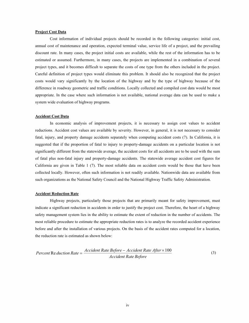
Project Cost Data

Cost information of individual projects should be recorded in the following categories: initial cost,

annual cost of maintenance and operation, expected terminal value, service life of a project, and the prevailing

discount rate. In many cases, the project initial costs are available, while the rest of the information has to be

estimated or assumed. Furthermore, in many cases, the projects are implemented in a combination of several

project types, and it becomes difficult to separate the costs of one type from the others included in the project.

Careful definition of project types would eliminate this problem. It should also be recognized that the project

costs would vary significantly by the location of the highway and by the type of highway because of the

difference in roadway geometric and traffic conditions. Locally collected and compiled cost data would be most

appropriate. In the case where such information is not available, national average data can be used to make a

system wide evaluation of highway programs.

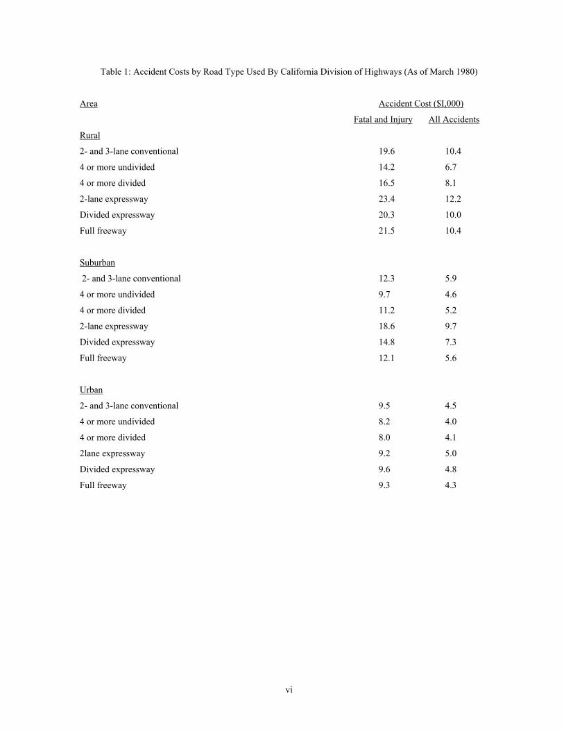
Accident Cost Data

In economic analysis of improvement projects, it is necessary to assign cost values to accident

reductions. Accident cost values are available by severity. However, in general, it is not necessary to consider

fatal, injury, and property damage accidents separately when computing accident costs (7). In California, it is

suggested that if the proportion of fatal to injury to property-damage accidents on a particular location is not

significantly different from the statewide average, the accident costs for all accidents are to be used with the sum

of fatal plus non-fatal injury and property-damage accidents. The statewide average accident cost figures for

California are given in Table 1 (7). The most reliable data on accident costs would be those that have been

collected locally. However, often such information is not readily available. Nationwide data are available from

such organizations as the National Safety Council and the National Highway Traffic Safety Administration.

Accident Reduction Rate

Highway projects, particularly those projects that are primarily meant for safety improvement, must

indicate a significant reduction in accidents in order to justify the project cost. Therefore, the heart of a highway

safety management system lies in the ability to estimate the extent of reduction in the number of accidents. The

most reliable procedure to estimate the appropriate reduction rates is to analyze the recorded accident experience

before and after the installation of various projects. On the basis of the accident rates computed for a location,

the reduction rate is estimated as shown below:

BeforeRateAccidentAfterRateAccidentBeforeRateAccidentRateductionPercent 100Re ×−

= (3)

v

The average value of reduction rate of a project type, r , can be obtained by weighted mean method, as

shown below:

b

ibi

m

i

n

rnrΣ== 1 (4)

where

m = number of locations where a particular: type of project has been implemented,

nb = total number of accidents before implementation of the project type in all locations.

vi

Table 1: Accident Costs by Road Type Used By California Division of Highways (As of March 1980)

Area Accident Cost ($I,000)

Fatal and Injury All Accidents

Rural

2- and 3-lane conventional 19.6 10.4

4 or more undivided 14.2 6.7

4 or more divided 16.5 8.1

2-lane expressway 23.4 12.2

Divided expressway 20.3 10.0

Full freeway 21.5 10.4

Suburban




2-lane expressway 18.6 9.7



Urban




2lane expressway 9.2 5.0



vii

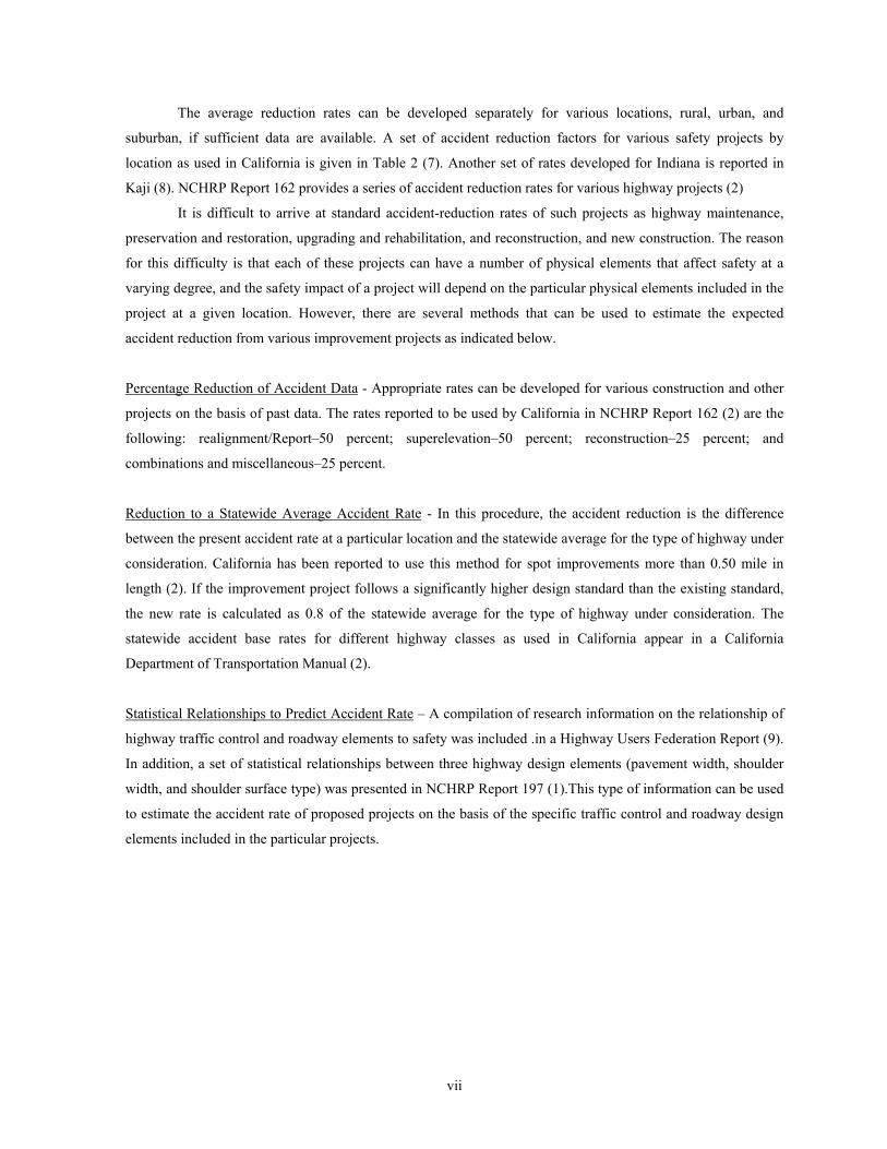
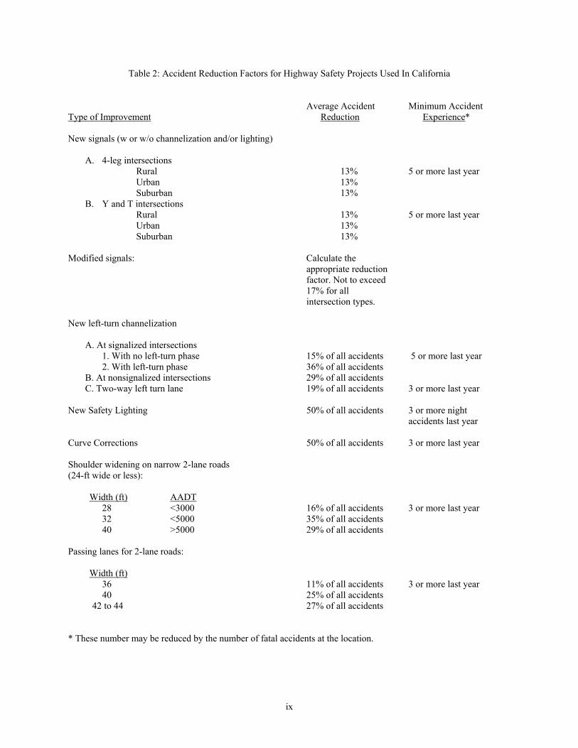
The average reduction rates can be developed separately for various locations, rural, urban, and

suburban, if sufficient data are available. A set of accident reduction factors for various safety projects by

location as used in California is given in Table 2 (7). Another set of rates developed for Indiana is reported in

Kaji (8). NCHRP Report 162 provides a series of accident reduction rates for various highway projects (2)

It is difficult to arrive at standard accident-reduction rates of such projects as highway maintenance,

preservation and restoration, upgrading and rehabilitation, and reconstruction, and new construction. The reason

for this difficulty is that each of these projects can have a number of physical elements that affect safety at a

varying degree, and the safety impact of a project will depend on the particular physical elements included in the

project at a given location. However, there are several methods that can be used to estimate the expected

accident reduction from various improvement projects as indicated below.

Percentage Reduction of Accident Data - Appropriate rates can be developed for various construction and other

projects on the basis of past data. The rates reported to be used by California in NCHRP Report 162 (2) are the

following: realignment/Report–50 percent; superelevation–50 percent; reconstruction–25 percent; and

combinations and miscellaneous–25 percent.

Reduction to a Statewide Average Accident Rate - In this procedure, the accident reduction is the difference

between the present accident rate at a particular location and the statewide average for the type of highway under

consideration. California has been reported to use this method for spot improvements more than 0.50 mile in

length (2). If the improvement project follows a significantly higher design standard than the existing standard,

the new rate is calculated as 0.8 of the statewide average for the type of highway under consideration. The

statewide accident base rates for different highway classes as used in California appear in a California

Department of Transportation Manual (2).

Statistical Relationships to Predict Accident Rate – A compilation of research information on the relationship of

highway traffic control and roadway elements to safety was included .in a Highway Users Federation Report (9).

In addition, a set of statistical relationships between three highway design elements (pavement width, shoulder

width, and shoulder surface type) was presented in NCHRP Report 197 (1).This type of information can be used

to estimate the accident rate of proposed projects on the basis of the specific traffic control and roadway design

elements included in the particular projects.

viii

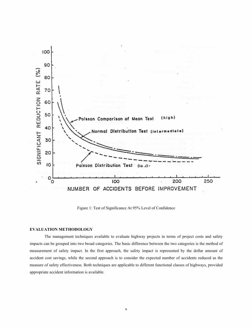
Significance Test of Accident Reduction Rate

Accidents are statically rare and random events. The number of accidents in a year is subject to normal

statistical variations. While dealing with small numbers, these variations can be large in terms of percentages.

For example, if a section of highway has experienced 10 accidents per year on the average, then it can be

expected that 85 percent of the time, the highway section would experience 5 to 15 accidents per year even

though no physical change is made in the highway section (7). Consequently, it is necessary to determine the

statistical significance of the expected accident reductions before further analysis is made.

There are several statistical tests to assess the significance of accident reduction effect of highway

improvement projects. One approach is to use the graphs shown in Figure 1 (2,8). The use of these graphs can be

illustrated with the following example. Let us assume a highway location has experienced 56 accidents per year

on the average in the past several years, and a safety improvement project proposed for this location has a

reduction rate of 45 percent. On the basis of the graph indicating an intermediate test, the significant reduction

rate for this location should be at least 30 percent for 95 percent level of confidence. As the expected reduction

rate is 45 percent, it can be concluded that it is significant at 95 percent level of confidence. However, if the

expected reduction rate were 25 percent, the same conclusion could not be made.

ix

Table 2: Accident Reduction Factors for Highway Safety Projects Used In California

Average Accident Minimum Accident Type of Improvement Reduction Experience* New signals (w or w/o channelization and/or lighting)

A. 4-leg intersections Rural 13% 5 or more last year Urban 13% Suburban 13%

B. Y and T intersections Rural 13% 5 or more last year Urban 13% Suburban 13%

Modified signals: Calculate the

appropriate reduction factor. Not to exceed 17% for all intersection types.

New left-turn channelization

A. At signalized intersections 1. With no left-turn phase 15% of all accidents 5 or more last year 2. With left-turn phase 36% of all accidents

B. At nonsignalized intersections 29% of all accidents C. Two-way left turn lane 19% of all accidents 3 or more last year

New Safety Lighting 50% of all accidents 3 or more night

accidents last year Curve Corrections 50% of all accidents 3 or more last year Shoulder widening on narrow 2-lane roads (24-ft wide or less): Width (ft) AADT

28 <3000 16% of all accidents 3 or more last year 32 <5000 35% of all accidents 40 >5000 29% of all accidents

Passing lanes for 2-lane roads: Width (ft)

36 11% of all accidents 3 or more last year 40 25% of all accidents

42 to 44 27% of all accidents * These number may be reduced by the number of fatal accidents at the location.

x

Figure 1: Test of Significance At 95% Level of Confidence

EVALUATION METHODOLOGY

The management techniques available to evaluate highway projects in terms of project costs and safety

impacts can be grouped into two broad categories. The basic difference between the two categories is the method of

measurement of safety impact. In the first approach, the safety impact is represented by the dollar amount of

accident cost savings, while the second approach is to consider the expected number of accidents reduced as the

measure of safety effectiveness. Both techniques are applicable to different functional classes of highways, provided

appropriate accident information is available.

xi

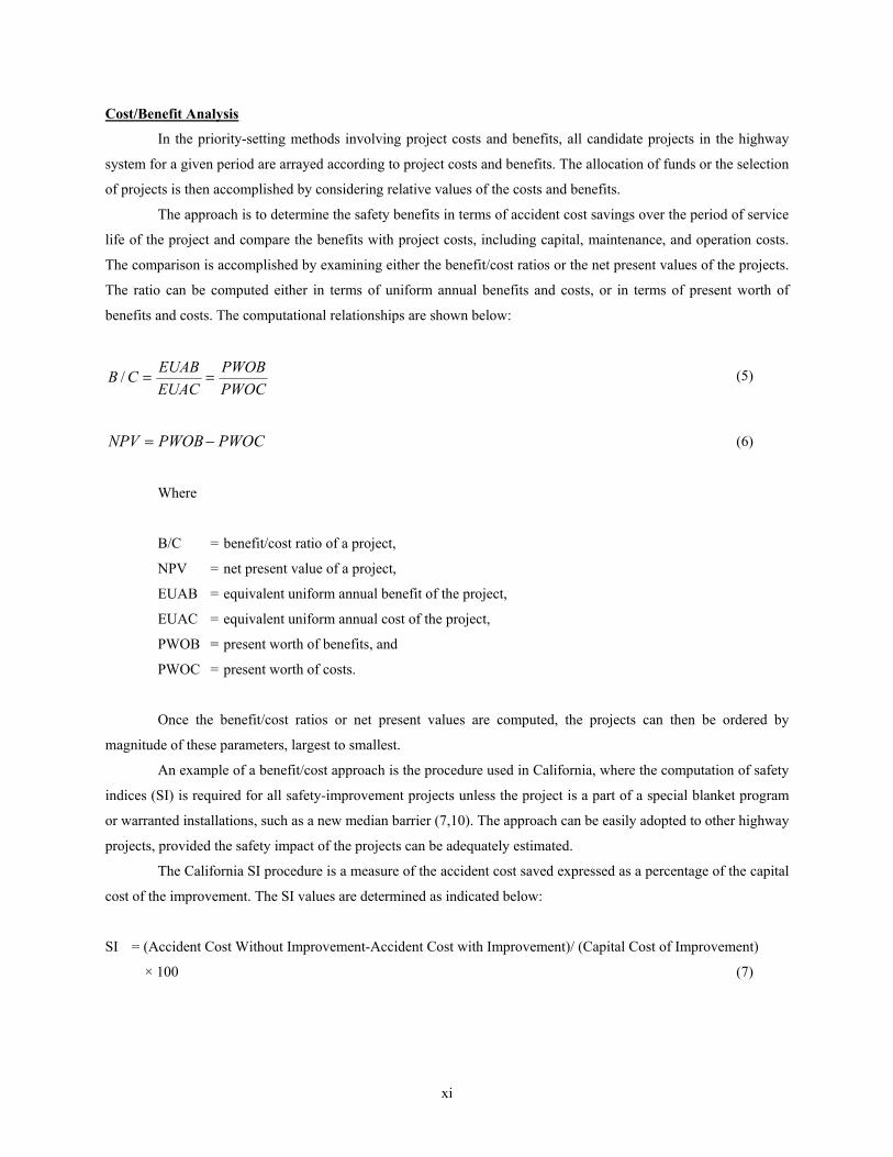
Cost/Benefit Analysis

In the priority-setting methods involving project costs and benefits, all candidate projects in the highway

system for a given period are arrayed according to project costs and benefits. The allocation of funds or the selection

of projects is then accomplished by considering relative values of the costs and benefits.

The approach is to determine the safety benefits in terms of accident cost savings over the period of service

life of the project and compare the benefits with project costs, including capital, maintenance, and operation costs.

The comparison is accomplished by examining either the benefit/cost ratios or the net present values of the projects.

The ratio can be computed either in terms of uniform annual benefits and costs, or in terms of present worth of

benefits and costs. The computational relationships are shown below:

PWOCPWOB

EUACEUABCB ==/ (5)

PWOCPWOBNPV −= (6)

Where

B/C = benefit/cost ratio of a project,

NPV = net present value of a project,

EUAB = equivalent uniform annual benefit of the project,

EUAC = equivalent uniform annual cost of the project,

PWOB = present worth of benefits, and

PWOC = present worth of costs.

Once the benefit/cost ratios or net present values are computed, the projects can then be ordered by

magnitude of these parameters, largest to smallest.

An example of a benefit/cost approach is the procedure used in California, where the computation of safety

indices (SI) is required for all safety-improvement projects unless the project is a part of a special blanket program

or warranted installations, such as a new median barrier (7,10). The approach can be easily adopted to other highway

projects, provided the safety impact of the projects can be adequately estimated.

The California SI procedure is a measure of the accident cost saved expressed as a percentage of the capital

cost of the improvement. The SI values are determined as indicated below:

SI = (Accident Cost Without Improvement-Accident Cost with Improvement)/ (Capital Cost of Improvement)

× 100 (7)

xii

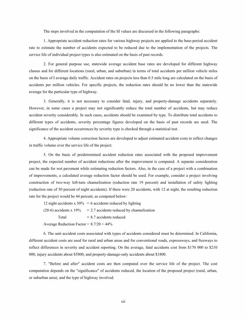
The steps involved in the computation of the SI values are discussed in the following paragraphs:

1. Appropriate accident reduction rates for various highway projects are applied to the base-period accident

rate to estimate the number of accidents expected to be reduced due to the implementation of the projects. The

service life of individual project types is also estimated on the basis of past records.

2. For general purpose use, statewide average accident base rates are developed for different highway

classes and for different locations (rural, urban, and suburban) in terms of total accidents per million vehicle miles

on the basis of I average daily traffic. Accident rates on projects less than 0.5 mile long are calculated on the basis of

accidents per million vehicles. For specific projects, the reduction rates should be no lower than the statewide

average for the particular type of highway.

3. Generally, it is not necessary to consider fatal, injury, and property-damage accidents separately.

However, in some cases a project may not significantly reduce the total number of accidents, but may reduce

accident severity considerably. In such cases, accidents should be examined by type. To distribute total accidents to

different types of accidents, severity percentage figures developed on the basis of past records are used. The

significance of the accident occurrences by severity type is checked through a statistical test.

4. Appropriate volume correction factors are developed to adjust estimated accident costs to reflect changes

in traffic volume over the service life of the project.

5. On the basis of predetermined accident reduction rates associated with the proposed improvement

project, the expected number of accident reductions after the improvement is computed. A separate consideration

can be made for wet pavement while estimating reduction factors. Also, in the case of a project with a combination

of improvements, a calculated average reduction factor should be used. For example, consider a project involving

construction of two-way left-turn channelization (reduction rate 19 percent) and installation of safety lighting

(reduction rate of 50 percent of night accidents). If there were 20 accidents, with 12 at night, the resulting reduction

rate for the project would be 44 percent, as computed below:

12 night accidents x 50% = 6 accidents reduced by lighting

(20-6) accidents x 19% = 2.7 accidents reduced by channelization

Total = 8.7 accidents reduced

Average Reduction Factor = 8.7/20 = 44%

6. The unit accident costs associated with types of accidents considered must be determined. In California,

different accident costs are used for rural and urban areas and for conventional roads, expressways, and freeways to

reflect differences in severity and accident reporting. On the average, fatal accidents cost from $170 000 to $210

000, injury accidents about $5800, and property-damage-only accidents about $1800.

7. "Before and after" accident costs are then computed over the service life of the project. The cost

computation depends on the "significance" of accidents reduced, the location of the proposed project (rural, urban,

or suburban area), and the type of highway involved.

xiii

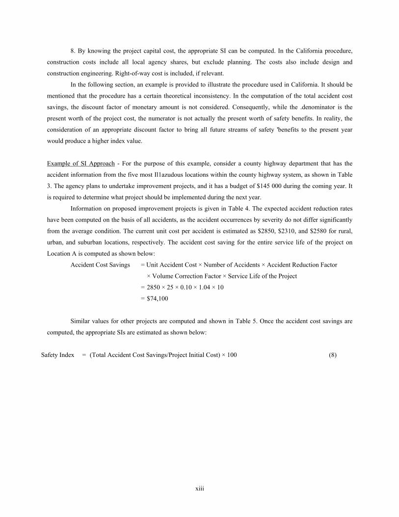
8. By knowing the project capital cost, the appropriate SI can be computed. In the California procedure,

construction costs include all local agency shares, but exclude planning. The costs also include design and

construction engineering. Right-of-way cost is included, if relevant.

In the following section, an example is provided to illustrate the procedure used in California. It should be

mentioned that the procedure has a certain theoretical inconsistency. In the computation of the total accident cost

savings, the discount factor of monetary amount is not considered. Consequently, while the .denominator is the

present worth of the project cost, the numerator is not actually the present worth of safety benefits. In reality, the

consideration of an appropriate discount factor to bring all future streams of safety 'benefits to the present year

would produce a higher index value.

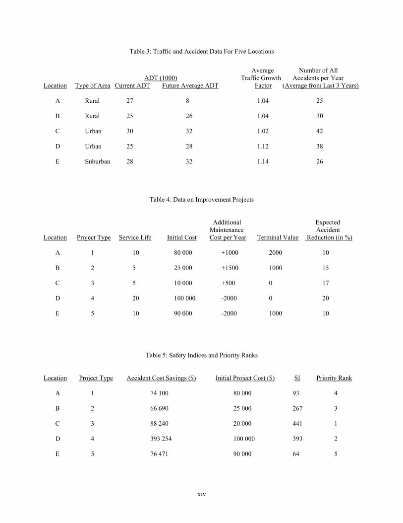
Example of SI Approach - For the purpose of this example, consider a county highway department that has the

accident information from the five most Il1azudous locations within the county highway system, as shown in Table

3. The agency plans to undertake improvement projects, and it has a budget of $145 000 during the coming year. It

is required to determine what project should be implemented during the next year.

Information on proposed improvement projects is given in Table 4. The expected accident reduction rates

have been computed on the basis of all accidents, as the accident occurrences by severity do not differ significantly

from the average condition. The current unit cost per accident is estimated as $2850, $2310, and $2580 for rural,

urban, and suburban locations, respectively. The accident cost saving for the entire service life of the project on

Location A is computed as shown below:

Accident Cost Savings = Unit Accident Cost × Number of Accidents × Accident Reduction Factor

× Volume Correction Factor × Service Life of the Project

= 2850 × 25 × 0.10 × 1.04 × 10

= $74,100

Similar values for other projects are computed and shown in Table 5. Once the accident cost savings are

computed, the appropriate SIs are estimated as shown below:

Safety Index = (Total Accident Cost Savings/Project Initial Cost) × 100 (8)

xiv

Table 3: Traffic and Accident Data For Five Locations

Average Number of All

ADT (1000) Traffic Growth Accidents per Year Location Type of Area Current ADT Future Average ADT Factor (Average from Last 3 Years) A Rural 27 8 1.04 25 B Rural 25 26 1.04 30 C Urban 30 32 1.02 42 D Urban 25 28 1.12 38 E Suburban 28 32 1.14 26

Table 4: Data on Improvement Projects

Additional Expected Maintenance Accident

Location Project Type Service Life Initial Cost Cost per Year Terminal Value Reduction (in %) A 1 10 80 000 +1000 2000 10 B 2 5 25 000 +1500 1000 15 C 3 5 10 000 +500 0 17 D 4 20 100 000 -2000 0 20 E 5 10 90 000 -2000 1000 10

Table 5: Safety Indices and Priority Ranks

Location Project Type Accident Cost Savings ($) Initial Project Cost ($) SI Priority Rank A 1 74 100 80 000 93 4 B 2 66 690 25 000 267 3 C 3 88 240 20 000 441 1 D 4 393 254 100 000 393 2 E 5 76 471 90 000 64 5

xv

The SIs for the five projects are indicated in Table 5. Using the SIs as the priority ratings, the rank orders of

the given projects are ascertained, and the array for these improvements is 3,4,2,1,5. However, projects with an SI

value of less than 100 should be dropped from further consideration. Furthermore, because the budget is limited to

$145 000, the first three improvement projects (on Locations C, D, and B) can be undertaken.

The California procedure uses an average level of future traffic for the entire study period to calculate total

safety benefits. However, the correct approach is to consider the safety benefits for each of the study years explicitly to

compute the discounted present worth of benefits (6). Furthermore, the California procedure does not consider the

lifecycle cost of a project. The additional annual cost, in some cases, may be positive, such as in the case of roadway

widening, shoulder widening, or installation of traffic control devices, guardrails, etc. In some situations, however, the

maintenance cost may decrease after improvement such as resurfacing or reconstruction.

In case of unequal project lives, it is necessary to consider a common analysis period. For example, let us

assume the analysis period in the problem considered here is 20 years. Then Projects 1 and 5 will have two cycles,

Projects 2 and 3, four cycles, and Project 4, only one cycle in the analysis period.

Assuming a terminal value at the end of the service life of a project, the present worth of cost for one cycle is

computed as:

Present Worth of Costs (PWOC) = Equivalent Uniform Annual Cost x Series Present Worth Factor (9)

where

Equivalent Uniform Annual Cost (EUAC) = Initial Project Cost × Capital Recovery Factor + Additional

Annual Cost of Maintenance and Operation - Terminal Value

× Sinking Fund Deposit Factor

For given discount rates and service life information, the values for capital recovery, sinking fund, and series

present worth factors can be obtained from standard tables (11).

The present worth of safety benefit in terms of accident cost savings is computed as:

Present Worth of Safety Benefits (PWOB) = First Year Benefits × Series Present Worth Factor (10)

where

First Year Benefits (FYB) = Number of Accidents Before Improvement per Year × Accident Reduction Rate

× Unit Cost of Accident

The benefits in the future years will change according to the change in traffic volume. For computation of

present worth of benefits, continuous compounding of first-year benefits to future years according to an annual rate of

growth of traffic volume is considered, and the future year benefits are then discounted to the present (6). The formula

for the series present worth factor is given below:

xvi

Continuously Compounded Exponential Series Present Worth Factor (CEPWF)

= ir

e nir

−−− 1)(

where

r = annual rate of growth of traffic volume,

i = discount rate in percent per year, and

n = analysis period.

The value of r can be obtained from Equation 12:

r = Year Future andYear BaseBetween Years ofNumber

ADT)Year Base ADTYear (Future Loge ÷ (12)

The 1977 AASHTO Manual on User Benefit Analysis (6) provides a simple chart that can be used to obtain

directly the present worth factors expressed in Equations 11 and 12.

Assuming a 10 percent discount rate, the computations for the equivalent uniform annual cost for

improvement project on Location A using Equation 9 are shown below:

EUAC = 80 000 × 0.162745 + 1000 - 2000 × 0.062745 = 13.894

The present worth of costs for this project, with a service life of 10 years, can then be computed by

considering two cycles of cash flows, assuming the analysis period is 20 years, as shown below:

PWOC = 13 894 × Uniform Series Present Worth Factor for 10% and 20 Years

= 13 894 × 8.51364 = 118 289

The computations for the present worth of safety benefits using Equations 10, 11, and 12 for Project 1 on

Location A are shown below:

FYB = 25 x 0.10 x 2850 = 7125

r = 5

0.007227)82( Loge =÷

(Future ADT given in Table 3 is for the middle of the project service life).

CEPWF = 0.10-0.0072

120)10.00072.0( −−e = 9.09163

PWOB = 7125 × 9.09163 = $64 778

xvii

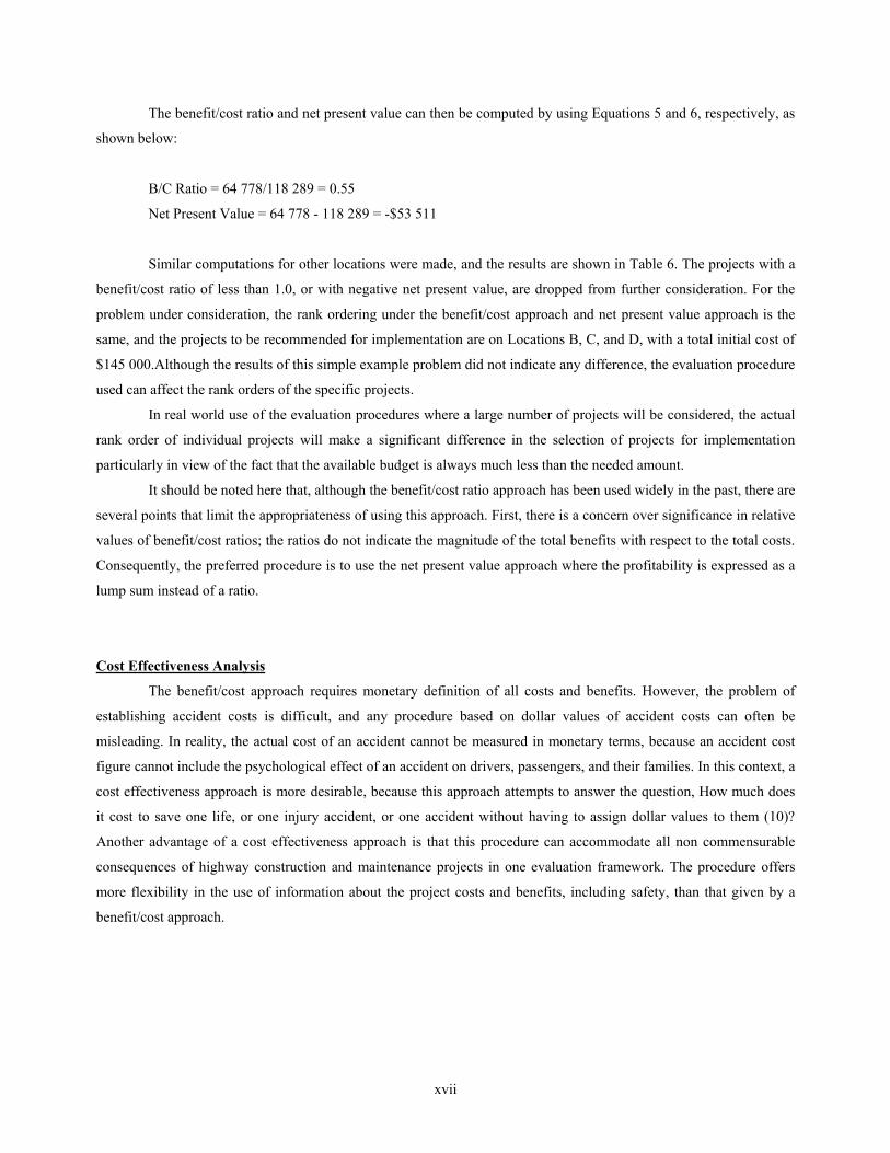
The benefit/cost ratio and net present value can then be computed by using Equations 5 and 6, respectively, as

shown below:

B/C Ratio = 64 778/118 289 = 0.55

Net Present Value = 64 778 - 118 289 = -$53 511

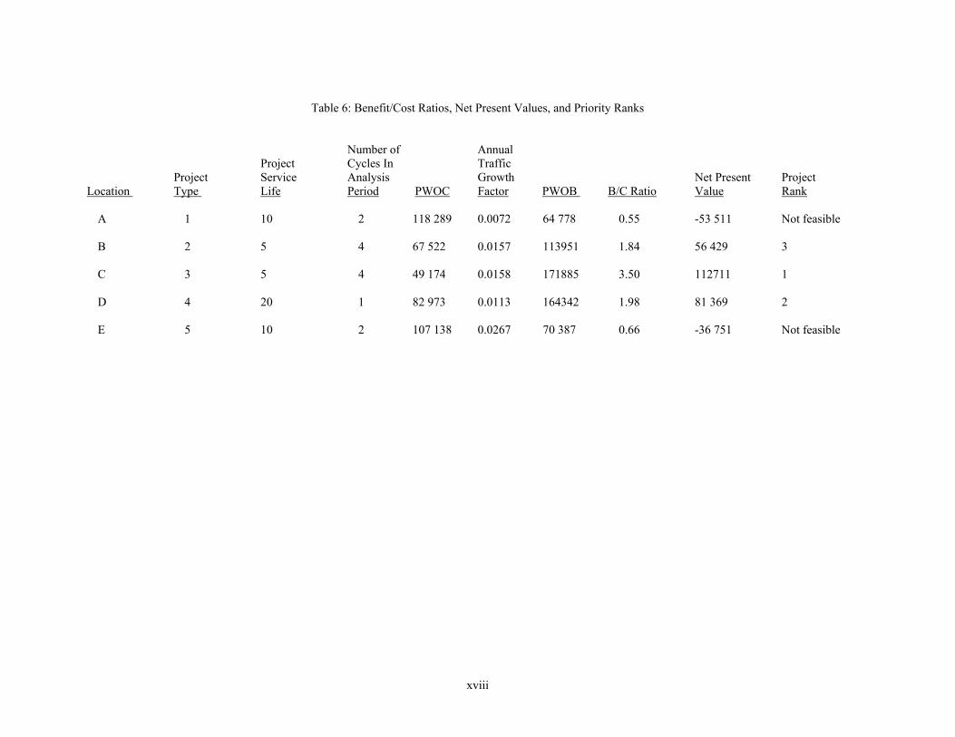
Similar computations for other locations were made, and the results are shown in Table 6. The projects with a

benefit/cost ratio of less than 1.0, or with negative net present value, are dropped from further consideration. For the

problem under consideration, the rank ordering under the benefit/cost approach and net present value approach is the

same, and the projects to be recommended for implementation are on Locations B, C, and D, with a total initial cost of

$145 000.Although the results of this simple example problem did not indicate any difference, the evaluation procedure

used can affect the rank orders of the specific projects.

In real world use of the evaluation procedures where a large number of projects will be considered, the actual

rank order of individual projects will make a significant difference in the selection of projects for implementation

particularly in view of the fact that the available budget is always much less than the needed amount.

It should be noted here that, although the benefit/cost ratio approach has been used widely in the past, there are

several points that limit the appropriateness of using this approach. First, there is a concern over significance in relative

values of benefit/cost ratios; the ratios do not indicate the magnitude of the total benefits with respect to the total costs.

Consequently, the preferred procedure is to use the net present value approach where the profitability is expressed as a

lump sum instead of a ratio.

Cost Effectiveness Analysis

The benefit/cost approach requires monetary definition of all costs and benefits. However, the problem of

establishing accident costs is difficult, and any procedure based on dollar values of accident costs can often be

misleading. In reality, the actual cost of an accident cannot be measured in monetary terms, because an accident cost

figure cannot include the psychological effect of an accident on drivers, passengers, and their families. In this context, a

cost effectiveness approach is more desirable, because this approach attempts to answer the question, How much does

it cost to save one life, or one injury accident, or one accident without having to assign dollar values to them (10)?

Another advantage of a cost effectiveness approach is that this procedure can accommodate all non commensurable

consequences of highway construction and maintenance projects in one evaluation framework. The procedure offers

more flexibility in the use of information about the project costs and benefits, including safety, than that given by a

benefit/cost approach.

xviii

Table 6: Benefit/Cost Ratios, Net Present Values, and Priority Ranks

Number of Annual Project Cycles In Traffic

Project Service Analysis Growth Net Present Project Location Type Life Period PWOC Factor PWOB B/C Ratio Value Rank A 1 10 2 118 289 0.0072 64 778 0.55 -53 511 Not feasible B 2 5 4 67 522 0.0157 113951 1.84 56 429 3 C 3 5 4 49 174 0.0158 171885 3.50 112711 1 D 4 20 1 82 973 0.0113 164342 1.98 81 369 2 E 5 10 2 107 138 0.0267 70 387 0.66 -36 751 Not feasible

xix

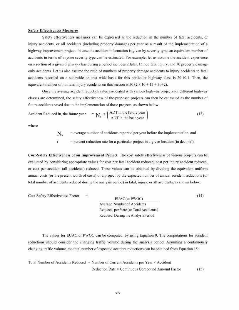
Safety Effectiveness Measures

Safety effectiveness measures can be expressed as the reduction in the number of fatal accidents, or

injury accidents, or all accidents (including property damage) per year as a result of the implementation of a

highway improvement project. In case the accident information is given by severity type, an equivalent number of

accidents in terms of anyone severity type can be estimated. For example, let us assume the accident experience

on a section of a given highway class during a period includes 2 fatal, 15 non fatal injury, and 30 property damage

only accidents. Let us also assume the ratio of numbers of property damage accidents to injury accidents to fatal

accidents recorded on a statewide or area wide basis for this particular highway class is 20:10:1. Then, the

equivalent number of nonfatal injury accidents on this section is 50 (2 x 10 + 15 + 30+2).

Once the average accident reduction rates associated with various highway projects for different highway

classes are determined, the safety effectiveness of the proposed projects can then be estimated as the number of

future accidents saved due to the implementation of these projects, as shown below:

Accident Reduced in, the future year =

⋅⋅

year base in the ADTyear future in the ADTrNb

(13)

where

Nb = average number of accidents reported per year before the implementation, and

r = percent reduction rate for a particular project in a given location (in decimal).

Cost-Safety Effectiveness of an Improvement Project The cost safety effectiveness of various projects can be

evaluated by considering appropriate values for cost per fatal accident reduced, cost per injury accident reduced,

or cost per accident (all accidents) reduced. These values can be obtained by dividing the equivalent uniform

annual costs (or the present worth of costs) of a project by the expected number of annual accident reductions (or

total number of accidents reduced during the analysis period) in fatal, injury, or all accidents, as shown below:

Cost Safety Effectiveness Factor =

Period Analysis theDuringReduced

) Accidents Total(or Year per ReducedAccidents ofNumber AveragePWOC)(or EUAC

(14)

The values for EUAC or PWOC can be computed. by using Equation 9. The computations for accident

reductions should consider the changing traffic volume during the analysis period. Assuming a continuously

changing traffic volume, the total number of expected accident reductions can be obtained from Equation 15:

Total Number of Accidents Reduced = Number of Current Accidents per Year × Accident

Reduction Rate × Continuous Compound Amount Factor (15)

xx

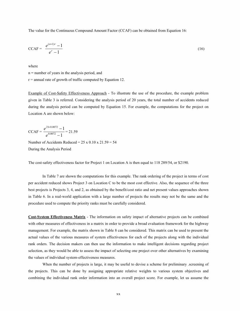
The value for the Continuous Compound Amount Factor (CCAF) can be obtained from Equation 16:

CCAF = 1

1)1(

−−+

r

rn

ee

(16)

where

n = number of years in the analysis period, and

r = annual rate of growth of traffic computed by Equation 12.

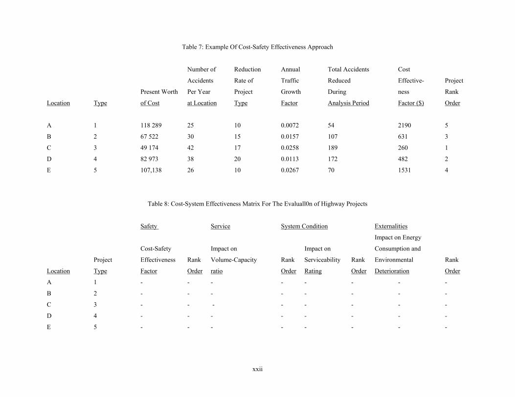
Example of Cost-Safety Effectiveness Approach - To illustrate the use of the procedure, the example problem

given in Table 3 is referred. Considering the analysis period of 20 years, the total number of accidents reduced

during the analysis period can be computed by Equation 15. For example, the computations for the project on

Location A are shown below:

CCAF = 11

0072.0

0072.021

−−×

ee

= 21.59

Number of Accidents Reduced = 25 x 0.10 x 21.59 = 54

During the Analysis Period

The cost-safety effectiveness factor for Project 1 on Location A is then equal to 118 289/54, or $2190.

In Table 7 are shown the computations for this example. The rank ordering of the project in terms of cost

per accident reduced shows Project 3 on Location C to be the most cost effective. Also, the sequence of the three

best projects is Projects 3, 4, and 2, as obtained by the benefit/cost ratio and net present values approaches shown

in Table 6. In a real-world application with a large number of projects the results may not be the same and the

procedure used to compute the priority ranks must be carefully considered.

Cost-System Effectiveness Matrix - The information on safety impact of alternative projects can be combined

with other measures of effectiveness in a matrix in order to provide a broad evaluation framework for the highway

management. For example, the matrix shown in Table 8 can be considered. This matrix can be used to present the

actual values of the various measures of system effectiveness for each of the projects along with the individual

rank orders. The decision makers can then use the information to make intelligent decisions regarding project

selection, as they would be able to assess the impact of selecting one project over other alternatives by examining

the values of individual system-effectiveness measures.

When the number of projects is large, it may be useful to devise a scheme for preliminary .screening of

the projects. This can be done by assigning appropriate relative weights to various system objectives and

combining the individual rank order information into an overall project score. For example, let us assume the

xxi

relative weights and the rank orders of the alternative projects with respect to each of the system-effectiveness

object1ves are as shown in Table 8. The safety objective is considered to be of highest priority, and therefore the

weight is 4. Condition is assumed to be of second highest priority, and service is given the third highest priority.

The objective related to energy and environment is considered to have the least priority.

The overall scare of an alternative Project J can be represented as:

ijii

j PwSCORE Σ=

where

jSCORE = overall scare of alternative project j,

iw = relative weight of system effectiveness objective i, and

ijP = rank order of alternative project j with respect to objective i.

The computation of the overall scare of alternative Project 1 by using Equation 17 is shown below:

SCORE 1 = w1 × P11 + W2 × P12 + w3 × P13 + w4 × P14 = 4 × 1 + 2 × 2 + 3 × 1 + 1 × 3 = 14

The overall project scare values of other alternative projects can be similarly computed and they are

shown in Table 9. It should be noted that in the example problem, the higher the score value, the higher is the rank

order. Therefore, the' best alternative is Project 3 on Location C, with an overall score of 42; while the least

attractive project is Project 1 on Location A, with an overall score of 14. With a given budget level, the top

projects can thus be sorted out in an ascending order of the project score values. Once the group of desirable

projects is selected, the actual sequence for the implementation of these projects can be determined through a

more detailed analysis of the system effectiveness information. In this analysis, the absolute values of the system

effectiveness objectives can be considered to evaluate the merit of one .project relative to other projects. It should

be noted that the weighting and ranking procedure often tends to over simplify the process of evaluation.

xxii

Table 7: Example Of Cost-Safety Effectiveness Approach

Number of Reduction Annual Total Accidents Cost

Accidents Rate of Traffic Reduced Effective- Project

Present Worth Per Year Project Growth During ness Rank

Location Type of Cost at Location Type Factor Analysis Period Factor ($) Order

A 1 118 289 25 10 0.0072 54 2190 5

B 2 67 522 30 15 0.0157 107 631 3

C 3 49 174 42 17 0.0258 189 260 1

D 4 82 973 38 20 0.0113 172 482 2

E 5 107,138 26 10 0.0267 70 1531 4

Table 8: Cost-System Effectiveness Matrix For The Evaluall0n of Highway Projects

Safety Service System Condition Externalities

Impact on Energy

Cost-Safety Impact on Impact on Consumption and

Project Effectiveness Rank Volume-Capacity Rank Serviceability Rank Environmental Rank

Location Type Factor Order ratio Order Rating Order Deterioration Order

A 1 - - - - - - - -

B 2 - - - - - - - -

C 3 - - - - - - - -

D 4 - - - - - - - -

E 5 - - - - - - - -

xxiii

Use of Optimization Approach in Project Selection

So far, discussion has involved the priority ranking of projects by using engineering economic and cost

effective approaches to develop priority arrays. However, there are several mathematical programming techniques that

can be effectively used in project selection and priority setting (12). The use of these techniques requires access to

computer facilities and may not be practical for some agencies.

For an efficient utilization of the resources, it may be necessary to evaluate alternative projects for all possible

locations simultaneously; and the management decision would be to select those projects that, on the whole, optimize

the safety effectiveness within the constraint of the available budget. In other words, the allocation of funds should be

made in such a way that the following question can be answered, what improvement projects should be undertaken in

what locations so that the safety effectiveness is maximized?

This problem can be solved by applying a simple integer programming technique (12). For example, if we consider that

safety effectiveness can be represented by the reduction of total accidents, the objective function of the problem can be

given as:

Maximize Z =ijijii XgrNAji ∈

∑∑ (18)

where

Ni = total number of accidents at location i;

rj = accident reduction rate of project j;

gi = growth rate factor of traffic volume for location i;

Xij = 1, if improvement project j is implemented at location, 0, otherwise; and

iAj∈ = improvement project j, which is one of a set of alternatives for location i, (Ai).

Equation 18 indicates that the total number of accidents can be minimized as a result of the system wide

implementation of highway projects. If sufficient information is available about the severity of accidents and the

reduction effect of alternative projects in terms of severity of accidents, the objective function can be appropriately

defined to minimize specific types of accidents.

As there are constraints imposed by the budget available, the following condition must be considered:

BXcAji ijiji ≥∈∑∑ (19)

ieachforXAj iji 1≤∈∑ (20)

xxiv

where

cij = initial cost of' the project j in location i, and

B = total budget available

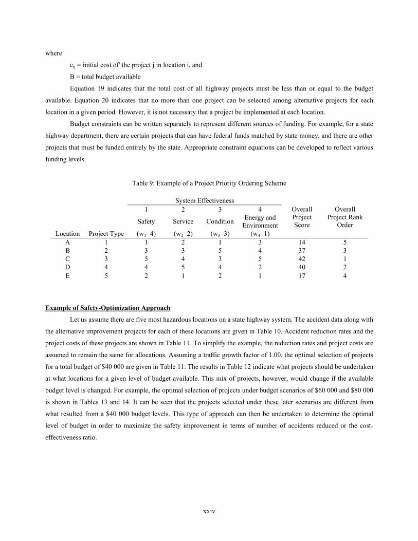
Equation 19 indicates that the total cost of all highway projects must be less than or equal to the budget

available. Equation 20 indicates that no more than one project can be selected among alternative projects for each

location in a given period. However, it is not necessary that a project be implemented at each location.

Budget constraints can be written separately to represent different sources of funding. For example, for a state

highway department, there are certain projects that can have federal funds matched by state money, and there are other

projects that must be funded entirely by the state. Appropriate constraint equations can be developed to reflect various

funding levels.

Table 9: Example of a Project Priority Ordering Scheme System Effectiveness

1 2 3 4 Safety Service Condition Energy and

Environment Location Project Type (w1=4) (w2=2) (w3=3) (w4=1)

Overall Project Score

Overall Project Rank

Order

A 1 1 2 1 3 14 5 B 2 3 3 5 4 37 3 C 3 5 4 3 5 42 1 D 4 4 5 4 2 40 2 E 5 2 1 2 1 17 4

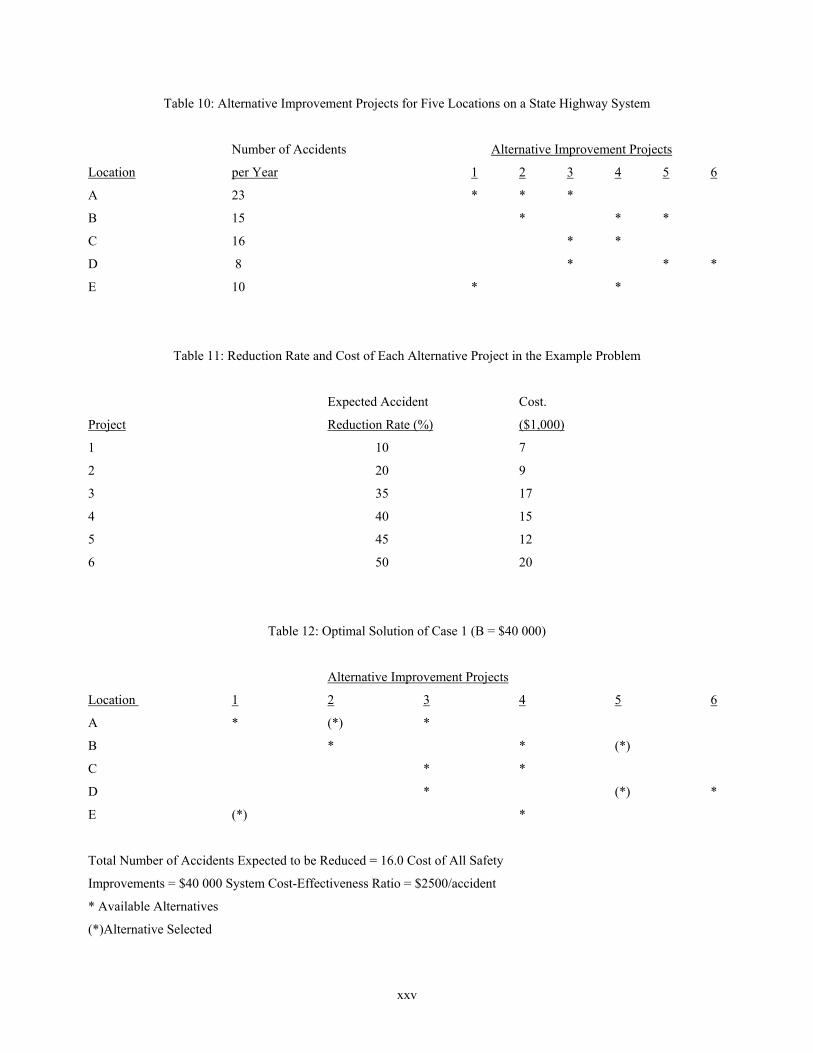
Example of Safety-Optimization Approach

Let us assume there are five most hazardous locations on a state highway system. The accident data along with

the alternative improvement projects for each of these locations are given in Table 10. Accident reduction rates and the

project costs of these projects are shown in Table 11. To simplify the example, the reduction rates and project costs are

assumed to remain the same for allocations. Assuming a traffic growth factor of 1.00, the optimal selection of projects

for a total budget of $40 000 are given in Table 11. The results in Table 12 indicate what projects should be undertaken

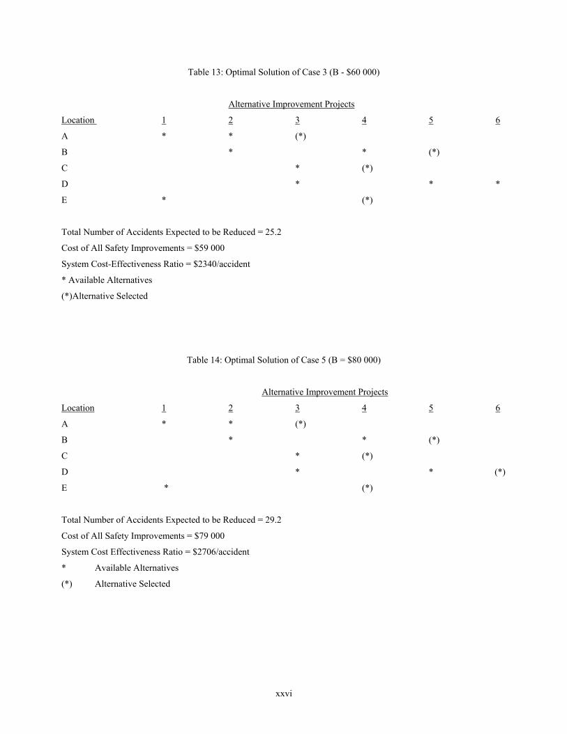
at what locations for a given level of budget available. This mix of projects, however, would change if the available

budget level is changed. For example, the optimal selection of projects under budget scenarios of $60 000 and $80 000

is shown in Tables 13 and 14. It can be seen that the projects selected under these later scenarios are different from

what resulted from a $40 000 budget levels. This type of approach can then be undertaken to determine the optimal

level of budget in order to maximize the safety improvement in terms of number of accidents reduced or the cost-

effectiveness ratio.

xxv

Table 10: Alternative Improvement Projects for Five Locations on a State Highway System

Number of Accidents Alternative Improvement Projects

Location per Year 1 2 3 4 5 6

A 23 * * *

B 15 * * *

C 16 * *

D 8 * * *

E 10 * *

Table 11: Reduction Rate and Cost of Each Alternative Project in the Example Problem

Expected Accident Cost.

Project Reduction Rate (%) ($1,000)

1 10 7

2 20 9

3 35 17

4 40 15

5 45 12

6 50 20

Table 12: Optimal Solution of Case 1 (B = $40 000)

Alternative Improvement Projects

Location 1 2 3 4 5 6

A * (*) *

B * * (*)

C * *

D * (*) *

E (*) *

Total Number of Accidents Expected to be Reduced = 16.0 Cost of All Safety

Improvements = $40 000 System Cost-Effectiveness Ratio = $2500/accident

* Available Alternatives

(*)Alternative Selected

xxvi

Table 13: Optimal Solution of Case 3 (B - $60 000)



A * * (*)

B * * (*)

C * (*)

D * * *

E * (*)

Total Number of Accidents Expected to be Reduced = 25.2

Cost of All Safety Improvements = $59 000

System Cost-Effectiveness Ratio = $2340/accident


(*)Alternative Selected

Table 14: Optimal Solution of Case 5 (B = $80 000)



A * * (*)

B * * (*)

C * (*)

D * * (*)

E * (*)

Total Number of Accidents Expected to be Reduced = 29.2

Cost of All Safety Improvements = $79 000

System Cost Effectiveness Ratio = $2706/accident


(*) Alternative Selected

xxvii

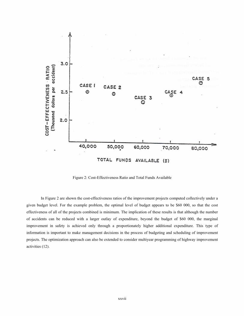
Figure 2: Cost-Effectiveness Ratio and Total Funds Available

In Figure 2 are shown the cost-effectiveness ratios of the improvement projects computed collectively under a

given budget level. For the example problem, the optimal level of budget appears to be $60 000, so that the cost

effectiveness of all of the projects combined is minimum. The implication of these results is that although the number

of accidents can be reduced with a larger outlay of expenditure, beyond the budget of $60 000, the marginal

improvement in safety is achieved only through a proportionately higher additional expenditure. This type of

information is important to make management decisions in the process of budgeting and scheduling of improvement

projects. The optimization approach can also be extended to consider multiyear programming of highway improvement

activities (12).

xxviii

Multiobjective Optimization of Highway Activities

The available highway funds are not adequate to undertake all the projects in keeping with accepted standards.

In the face of limited resources, the issue is how to make the best use of limited funds. The solution obviously lies in

compromising improvement and maintenance efforts either in quality or quantity or both (13). The highway

management decision is to determine the optimal strategy that would yield the maximum benefit within the constraint

of budget availability. In this effort, there are several objectives that an effective highway system management must

consider. Highway improvement and maintenance activities are undertaken to improve roadway condition, provide a

higher level of service, enhance safety, and reduce energy conservation and environmental pollution. The highway

management decisions involve how to determine what apportionment scheme of the available limited funds will enable

the achievement of as many system objectives as possible, to as great an extent as possible, for as long as possible.

The optimization technique discussed so far involved a single objective, safety without considering the role of

other objectives. However, in the real world, the problem is of a multiobjective decision situation. A procedure has

been developed on the basis of a multiobjective optimization approach to allocate optimally the limited highway

resources (14). In this approach, targets or goals are assigned for each of the identified objectives, and the goal-

programming algorithm determines a solution that comes “as close as possible” to all the given goals or targets. In the

following section, a brief discussion of the application of this procedure is presented. Detailed information on this

technique can be obtained in Sinha and others (14).

The procedure was applied to the Indiana highway system as reported in the 1976 National Highway

Inventory and Performance Summary (15). The highway system was divided into six classes, and all possible highway

activities were grouped into seven categories. The physical and traffic inventory of the highway system is considered

along with given design and maintenance standards to determine the deficient miles and the feasible alternative

projects. The impact of each type of project on each of the four major system objectives was derived through an

opinion survey of a group of highway engineering design and maintenance personnel. The format of a matrix that

indicates the relative role each of the activities play in achieving each of the system objectives is given in Table 15.

This matrix can be developed through a field survey supplemented by the empirical evidence reported in the literature.

The coefficients of the matrix should reflect the difference in useful life of each of the projects. A separate matrix can

be developed for each of the six highway categories considered.

With a given level of budget including state funds and federal grants, with associated matching requirements,

and with a given set of targets for each of the stated objectives assigned by the highway system management, the

procedure is to allocate available funds in order to determine miles of highway in each class to undergo a particular

highway activity during a certain analysis period. Each of the system objectives is assigned a priority rating that affects

the choice of type and r location of projects. For example, the management may decide that highway, safety is most

critical compared with other objectives, and the priorities can then be set accordingly.

The difference in programming strategies dictated by the difference in priorities assigned to system objectives

can be studied by the results of the goal programming optimization algorithm. For example, a particular case study

indicated that by assigning safety higher priority, the highway management strategy lies in reducing the resurfacing

activity to a small extent on urban other arterials and considerably on rural other arterials. The released money is

diverted to do all the needed minor widening in these classes of highways. Also, the needed traffic engineering

xxix

improvements are undertaken on rural interstates to fulfill the safety objective. It should be noted, however, that the

specific details of the management strategy would depend on the actual input information provided for system weights,

objective priorities, unit project cost data, and other required parameters.

Risk Analysis

The input information used in the evaluation techniques may be associated with a certain degree of

uncertainty. In some cases, a small change in the estimated values of cost, accident reduction, or any other data used in

the evaluation process can alter the results significantly. If the reliability of the input data is not high, it is advisable that

a series of computations be made to test the effects of possible errors in the estimates of the input data, including cost

and safety Impacts. The test can be conducted with a range of possible values for the key input data. For example,

average values are generally considered for the unit project cost figures r and accident reduction rates. However, these

values may have a large variance in rank orders of various candidate projects in a priority setting process, the cost

effectiveness technique is recommended, because the problem of establishing accident costs can be difficult. The

results based on dollar values of accident costs may be misleading.

In addition to traditional techniques, approaches based on mathematical programming techniques can be

employed to ensure optimal allocation of limited resources. Priority ranking of projects and selecting projects from the

top of the list until the available fund is exhausted may not yield optimal use of the funds. A systematic procedure

based on integer programming techniques can be undertaken to select both the project type and its location. This way,

the total safety effectiveness is maximized within the constraint of available resources. This approach will optimize

only one objective, that is, safety. However, a highway system manager must consider other objectives. In fact, the

highway management decision making is a multiobjective problem.

A comprehensive highway system management and programming tool can be used to identify strategies

involving the selection of various improvement and maintenance projects throughout the highway system. These

strategies should maximize safety effectiveness while satisfying the stated goals of improving highway condition and

service while reducing energy consumption and environ mental pollution, within the limitation of available funds. Such

a procedure would be of much use in selecting optimal highway programming strategies under a series of funding and

policy scenarios.

It should be noted that all of the techniques reviewed in this paper are not equally applicable at all levels of

government. For example, for many county and other local highway agencies, without access to adequate computer

facilities or enough detailed data, it is not advisable or necessary to adopt a mathematical programming approach to

optimize its highway funds, unless the funding amount is large and the number of needed projects is too large. For

these agencies and also for many state highway agencies, priority arraying using the cost effectiveness approach would

be an adequate tool. However, agencies with the capability to maintain an elaborate data management system and with

access to computer facilities, the use of an optimization approach may be desirable, particularly in view of the fact that

the techniques discussed provide a comprehensive approach to the programming process

Highway safety is a complex and critical issue. Careful implementation of highway improvement and

maintenance projects involving appropriate roadway elements can make a significant contribution to highway safety. It

is therefore necessary to adopt appropriate management techniques that would ensure that the safety aspects of the

xxx

candidate highway projects are critically evaluated. Limited highway funds must be allocated optimally so that the

safety effectiveness is maximized without jeopardizing the other system objectives.

Table 15: Matrix Indicating Impact of Various Highway Activities on System Objectives

Activity Objective

Reconstruction Major Widening Minor Widening Resurfacing Traffic engineering

Improvements Routine

Maintenance

Condition -- -- -- -- -- --

Service -- -- -- -- -- --

Safety -- -- -- -- -- --

Energy and Environment -- -- -- -- -- --

xxxi

ACKNOWLEDGMENT

I acknowledge the assistance of c. c. Liu and E. Sharaf in checking my computations and of Marion Sipes in typing the

paper. I am also thankful to Carlton Robinson and Harold L. Michael for their suggestions.

REFERENCES

1. Cost and Safety Effectiveness of Highway Design Elements. NCHRP Report 197, Transportation Research

Board, 1978.

2. Methods for Evaluating Highway Safety Improvements. NCHRP Report 162, Transportation Research Board,

1975.

3. Priority Programming and Project Selection. NCHRP Synthesis of Highway Practice Report 48,

Transportation Research Board, 1978.

4. Capital Project Priority Process Manual. California Department of Transportation, Division of Highways,

March 30, 1981.

5. K. C. Sinha and D. P. Jukins. Project Evaluation and Priority Programming Criteria. Transportation Research

Circular 213, 1980.

6. A Manual on User Benefit Analysis of Highway and Bus Transit Improvements. AASHTO, 1977.

7. Safety Evaluation. California Department of Transportation, Departmental Memorandum, May 1980.

8. T. Kaji. A Cost-Effectiveness Approach for the Evaluation of Highway Safety Improvements in the State of

Indiana. Joint Highway Research Project No. C-36-73J, School of Civil Engineering, Purdue University,

1980.

9. Traffic Control and Roadway Elements - Their Relationship to Safety. Highway Users Federation, 1968-1971.

10. T. N. Tamburri and R. N. Smith. The Safety Index: A Method of Evaluating and Rating Safety Benefits.

Highway Research Record 332, 1970.

11. R. Winfrey. Economic Analysis for Highways. International Textbook Company, Scranton, PA, 1969.

12. K. C. Sinha, T. Kaji, and C. C. Liu. Optimal Allocation of Funds for Highway Safety Improvement Projects.

Paper presented at 60th Annual. Meeting of the Transportation Research Board, January 1981.

13. R. R. Knox and others. Programming Highway Improvements in New Funding Environment. Transportation

Research Record 599, 1976.

14. K. C. Sinha, A. Ravindran, and M. Muthuwbramanyam. Optimal Allocation of Funds for the Maintenance and

Preservation of the Existing Highway System. Automotive Transportation Center, Purdue University, Sept.

1980.

15. The National Highway Inventory and Performance Summary. U. S. Department of Transportation, Federal

Highway Administration, Dec. 1977.

Documents

HIGHWAY PROGRAMING, INFORMATION MANAGEMENT …