Embed Size (px)
Citation preview
Hilbert Spaces, Wavelets, Generalised Functions and Modem Quantum Mechanics
Mathematics and Its Applications
Managing Editor:
M. HAZEWINKEL Centre for Mathematics and Computer Science, Amsterdam, The Netherlands
Volume 451
Hilbert Spaces, Wavelets, Generalised Functions and Modem Quantum Mechanics
by
Willi-Hans Steeb
International Schoolfor Scientijic Computing, Rand Afriwns University, JohIJnnesburg, South Africa
SPRINGER-SCIENCE+BUSINESS MEDIA, B.V.

A C.I.P. Catalogue record for this book is available from the Library of Congress.
ISBN 978-94-010-6241-1 ISBN 978-94-011-5332-4 (eBook) DOI 10.1007/978-94-011-5332-4
Reprinted with corrections First published 1998, reprinted 2000
Printed on acid-free paper
AII Rights Reserved © 1998 Springer Science+ Business Media Dordrecht Originally published by Kluwer Academic Publishers in 1998 Softcover reprint ofthe hardcover Ist edition 1998 No part of the material protected by this copyright notice may be reproduced or utilized in any form or by any means, electronic or mechanical, including photocopying, recording or by any information storage and retrieval system, without wrltten permission from the copyright owner
Contents
1 Hilbert Spaces
2 Fourier Transform and Wavelets
3 Linear Operators in Hilbert Spaces
4 Generalized Functions
5 Classical Mechanics and Hamilton Systems
6 Postulates of Quantum Mechanics
7 Interaction Picture
8 Eigenvalue Problem 8.1 Eigenvalue Equation .............. . 8.2 Applications ................... .
8.2.1 Free Particle in a One-Dimensional Box. 8.2.2 8.2.3 8.2.4
Rotator ................. . Free Particle in a Bounded n-Dimensional Region Two Dimensional Examples . . . . . . . . . . . .
9 Spin Matrices and Kronecker Product
10 Parity and Group Theory
11 Uncertainty Relation
12 Harmonic Oscillator 12.1 Classical Case . 12.2 Quantum Case ..
13 Coherent and Squeezed States
1
17
31
51
63
69
77
85 85 86 86 89 92 95
101
109
117
123 . 123 . 125
135
14 Angular Momentum and Lie Algebras
15 Two-Body Bound State Problem 15.1 Introduction ..... 15.2 Spherical Oscillator. 15.3 Hydrogen-like Atoms
16 One-Dimensional Scattering
17 Solitons and Quantum Mechanics
18 Perturbation Theory
19 Helium Atom
20 Potential Scattering
21 Berry Phase
22 Measurement and Quantum States 22.1 Introduction ........ . 22.2 Measurement Problem .. . 22.3 Copenhagen Interpretation. 22.4 Hidden Variable Theories. 22.5 Everett Interpretation .. 22.6 Basis Degeneracy Problem
23 Quantum Computing 23.1 Introduction .. 23.2 Quantum Bit . . . 23.3 Quantum Gates . . 23.4 Quantum Copying 23.5 Shor's Algorithm .
24 Lebesgue Integration and Stieltjes Integral
Bibliography
Index
141
149 .149 · 150 · 153
157
165
171
179
183
189
195 · 195 · 196 .197 .200 .201 .203
205 · 205 .206 .207 · 212 .214
217
225
231
List of Symbols
o N Z Q R R+ e Rn en 1l i ~z C;SZ AcB AnB AuB fog 1/;, I1/;) t x xERn
11·11 xx y ® 1\
(,), (I) det tr {, } ['l [, l+ 15jk
8 sgn(x) A
empty set natural numbers integers rational numbers real numbers nonnegative real numbers complex numbers n-dimensional Euclidian space n-dimensional complex linear space Hilbert space :=A real part of the complex number z imaginary part of the complex number z subset A of set B the intersection of the sets A and B the union of the sets A and B composition of two mappings (f 0 g)(x) = f(g(x)) wave function independent variable (time variable) independent variable (space variable) element x of Rn norm vector product Kronecker product, tensor product exterior product (Grassmann product, wedge product) scalar product (inner product) determinant of a square matrix trace of a square matrix Poisson product commutator anticommutator Kronecker delta delta function the sign of x, 1 if x > 0, -1 if x < 0, 0 if x = 0 eigenvalue real parameter
I U II H iI v bj , b{ Cj, cj
p
P L L i,8) D f2+ Yim(O, ¢)
unit operator, unit matrix unitary operator, unitary matrix projection operator, projection matrix Hamilton function Hamilton operator potential Bose operators Fermi operators momentum momentum operator angular momentum angular momentum operator Bose coherent state differential operator a/ax M011er operator spherical harmonics
Preface
This book provides an introduction to Hilbert space theory, Fourier transform and wavelets, linear operators, generalized functions and quantum mechanics. Although quantum mechanics has been developed between 1925 and 1930 in the last twenty years a large number of new aspect and techniques have been introduced. The book also covers these new fields in quantum mechanics.
In quantum mechanics the basic mathematical tools are the theory of Hilbert spaces, the theory of linear operators, the theory of generalized functions and Lebesgue integration theory. Many excellent textbooks have been written on Hilbert space theory and linear operators in Hilbert spaces. Comprehensive surveys of this subject are given by Weidmann [68], Prugovecki [47], Yosida [69], Kato [31], Richtmyer [49], Sewell [54] and others. The theory of generalized functions is also well covered in good textbooks (Gelfand and Shilov [25], Vladimirov [67]. Furthermore numerous textbooks on quantum mechanics exist (Dirac [17], Landau and Lifshitz [36], Messiah [41], Gasiorowicz [24], Schiff [51], Eder [18] and others). Besides these books there are several problem books on quantum mechanics (Fliigge [22], Constantinescu and Magyari [15], ter Haar [64], Mavromatis [39], Steeb [59], Steeb [60], Steeb [61]) and others). Computer algebra implementations of quantum mechanical problems are described by Steeb [59].
Unfortunately, many standard textbooks on quantum mechanics neglect the mathematical background. The basic mathematical tools to understand quantum mechanics should be fully integrated into an education in quantum mechanics.
The first four chapters of this book give an introduction to the mathematical tools necessary in quantum mechanics. The remaining chapters are devoted to quantum mechanics. The final chapter gives an introduction to Lebesgue integration theory.
The book covers new fields in quantum mechanics, such as coherent states, squeezed states, solitons and quantum mechanics, secular terms, Kronecker product and spin systems, and Berry phase, perturbation theory and differential equations, quantum measurement and quantum computing. These fields are not included in many standard textbooks in quantum mechanics.
Basic knowledge in linear algebra and calculus is required. It is also desirable for the reader to have basic knowledge in Hamilton mechanics. In almost all chapters a large number of examples serve to illustrate the mathematical tools. Most of the chapters include several exercises. A large number of references are given for further reading.
Ends of proofs are indicated by.. Ends of examples are indicated by •.
Any useful suggestions and comments are welcome. The e-mail address of the author is:
The web page of the author is:
http://zeus.rau.ac.za/steeb/steeb/html
While writing this book I have received encouragement from many sources. In particular I would like to acknowledge my special indebtedness to Prof. Peter Mulser and Prof. Ruedi Stoop. Special thanks are due to John and Catharine Thompson who proofread the final manuscript.
Chapter 1
Hilbert Spaces
In this chapter we introduce the Hilbert space which plays the central role in quantum mechanics. For a more detailed discussion of this subject we refer to the books of Stakgold [58], Sewell [54], Yosida [69], Richtmyer [49], Weidmann [68], Balakrishnan [3]. Moreover the proofs of the theorems given in this chapter and chapter 2 can be found in these books. We assume that the reader is familiar with the notation of a linear space. First we introduce the pre-Hilbert space.
Definition. A linear space L is called a pre-Hilbert space if there is defined a numerical function called the scalar product (or inner product) which assigns to every i, 9 of vectors of L (J, gEL) a complex number C. The scalar product satisfies the conditions
(a) (1,1) ? 0 (1, 1) = 0 iff i = 0
(b) (1, g) = (g,1)
(c) (ci, g) = c(1, g) where c is an arbitrary complex number
(d) (II + h g) = (II, g) + (12, g)
where (g,1) denotes the complex conjugate of (g,1).
It follows that
and
(1, cg) = c(1, g).
1
W.-H. Steeb, Hilbert Spaces, Wavelets, Generalised Functions and Modern Quantum Mechanics© Kluwer Academic Publishers 1998
2 CHAPTER 1. HILBERT SPACES
Definition. A linear space E is called a normed space, if for every ! E E there is associated a real number II!II, the norm of the vector! such that
(a) II!II ~ 0, II!II = 0 iff ! = 0
(b) Ilc!11 = lelll!11 where e is an arbitrary complex number
(e) II! + gil :S II!II + Ilgll·
The conditions imply that
II! - gil ~ III!II- Ilglll·
This can be seen as follows. From
II! - gil + Ilgll ~ II!II
we obtain
II! - gil ~ II!II- Ilgll·
On the other hand
II! - gil = 1- Illig - !II ~ IlglI-II!II·
The topology of a normed linear space E is thus defined by the distance
dU,g) = II! - gil·
If a scalar product is given we can introduce a norm. The norm of ! is defined by
II!II := J(f, f}.
A vector! E L is called normalized if Ilfll = 1.
Definition. Two functions ! ELand gEL are called orthogonal if
(f,g) = O.
Example. Consider the pre-Hilbert space R4 and
3
Definition. A sequence {fn} (n E N) of elements in a normed space E is called a Cauchy sequence if, for every f > 0, there exists a number Mf such that IIfp - fqll < f
for p,q > M f •
Example. The sequence
n-l 1 fn = L k'
k=O •
is a Cauchy sequence. ..
Definition. A normed space E is said to be complete if every Cauchy sequence of elements in E converges to an element in E.
Example. Let Q be the rational numbers. Since the sum and product of two rational numbers are again rational numbers we obviously have a pre-Hilbert space with the scalar product (qI, q2) := qlq2. However, the pre-Hilbert space is not complete. Consider the sequence
1 1 1 fn = 1 + iT + 2! + ... + (n - I)!
with n = 1,2, .... The sequence fn is obviously a Cauchy sequence. However
lim fn --+ e n-+oo
and e f/. Q. ..
Definition. A complete pre-Hilbert space is called a Hilbert space.
Definition. A complete normed space is called a Banach space.
Example. The vector space C([a, bJ) of all continuous (real or complex valued) functions on an interval [a, b] with the norm
is a Banach space. ..
IIfll = max If(x)1 [a,]
A Hilbert space will be denoted by 1l in the following. A Banach space will be denoted by B in the following.
Theorem. Every pre-Hilbert space L admits a completion 1l which is a Hilbert space.
4 CHAPTER 1. HILBERT SPACES
Example. Let L = Q. Then H = R. '"
Before we discuss some examples of Hilbert spaces we give the definitions of strong and weak convergence in Hilbert spaces.
Definition. A sequence {in} of vectors in a Hilbert space H is said to converge strongly to i if
Illn - ill --+ 0
as n --+ 00. We write s - limn~oo in --+ f.
Definition. A sequence {In} of vectors in a Hilbert space H is said to converge weakly to I if
Un' g) --+ U, g)
as n --+ 00, for any vector g in H. We write w - limn~oo in --+ f.
It can be shown that strong convergence implies weak convergence. The converse is not generally true, however.
Example. Consider the sequence
in(x) := sin(nx), n = 1,2, ...
in the Hilbert space L2 [0, ?fl. The sequence does not tend to a limit in the sense of strong convergence. However, the sequence tends to 0 in the sense of weak convergence. '"
Let us now give several examples of Hilbert spaces which are important in quantum mechanics.
Example 1. Every finite dimensional vector space with an inner product is a Hilbert space. Let en be the linear space of n-tuples of complex numbers with the scalar product
n
(u, v) := I>jVj. j=1
Then en is a Hilbert space. Let u E en. We write the vector u as a column vector
Thus we can write the scalar product in matrix notation
5
(u, v) = uT "
where uT is the transpose of u. ..
Example 2. By l2(N) we mean the set of all infinite dimensional vectors (sequences) u = (UI, U2, . .. f of complex numbers Uj such that
00
2: IUjl2 < 00. j=1
Here l2 (N) is a linear space with operations (a E C)
au (aU1' aU2,···f
u+v (U1 + VI, U2 + V2, ... )T
00 00 00
2: IUj + Vjl2 :s 2:(IUjI2 + IVjl2 + 2lujvjl) :s 2 2:(lujI2 + IVjI2) < 00. j=l j=1 j=l
The scalar product is defined as
00
(u, v) := I: UjVj = UT". j=l
It can also be proved that this pre-Hilbert space is complete. Therefore l2(N) is a Hilbert space. As an example, let us consider
1 lIT U = (1, -, -, ... , -, ... ) .
2 3 n
Since
we find that u E l2 (N). Let
6 CHAPTER 1. HILBERT SPACES
Example 3. L2(M) is the space of Lebesgue square-integrable functions on M, where M is a Lebesgue measurable subset of R n , where n E N. If f E L 2 (M), then
J Ifl2 dm < 00.
M
The integration is performed in the Lebesgue sense. The scalar product in L2(M) is defined as
(j, g) := J f(x)g(x) dm M
where 9 denotes the complex conjugate of g. It can be shown that this pre-Hilbert space is complete. Therefore L2 (M) is a Hilbert space. Instead of dm we also write dx in the following. If the Riemann integral exists then it is equal to the Lebesgue integral. However, the Lebesgue integral exists also in cases in which the Riemann integral does not exist. For details of Lebesgue integration we refer to chapter 21. .. Example 4. Consider the linear space Mn of all n x n matrices over C. The trace of an n x n matrix A = (ajk) is given by
n
trA = L ajj. j=1
We define a scalar product by
(A, B) := tr(AB*)
where tr denotes the trace and B* denotes the conjugate transpose matrix of B. We recall that tr( C + D) = trC + trD where C and Dare n x n matrices. ..
Example 5. Consider the linear space of all infinite dimensional matrices A = (ajk)
over C such that
00 00
L L lajkl 2 < 00. j=lk=l
We define a scalar product by
(A, B) := tr(AB*)
where tr denotes the trace and E* denotes the conjugate transpose matrix of E. We recall that tr( C + D) = trC + trD where C and D are infinite dimensional matrices. The infinite dimensional unit matrix does not belong to this Hilbert space. ..
Example 6. Let D be an open set of the Euclidean space Rn. Now L2 (D)pq denotes the space of all q x p matrix functions Lebesgue measurable on D such that
! trf(x)f(x)*dm < 00
D
7
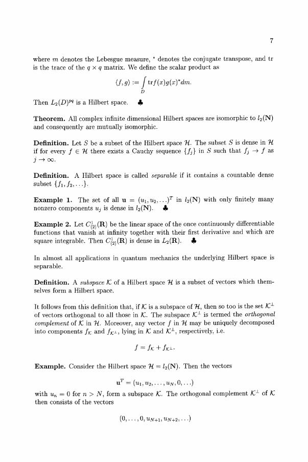
where m denotes the Lebesgue measure, * denotes the conjugate transpose, and tr is the trace of the q x q matrix. We define the scalar product as
(1, g) := J tr/(x)g(x)*dm. D
Then L2(D)pq is a Hilbert space. '"
Theorem. All complex infinite dimensional Hilbert spaces are isomorphic to 12(N) and consequently are mutually isomorphic.
Definition. Let S be a subset of the Hilbert space 1i. The subset S is dense in 1i if for every I E 1i there exists a Cauchy sequence {lj} in S such that Ij ---+ I as j ---+ 00.
Definition. A Hilbert space is called separable if it contains a countable dense subset {II, h .. . }.
Example 1. The set of all u = (UI, U2," Y in 12(N) with only finitely many nonzero components Uj is dense in 12(N). '"
Example 2. Let 0(2) (R) be the linear space of the once continuously differentiable functions that vanish at infinity together with their first derivative and which are square integrable. Then q2)(R) is dense in L2(R). '"
In almost all applications in quantum mechanics the underlying Hilbert space is separable.
Definition. A subspace K of a Hilbert space 1i is a subset of vectors which themselves form a Hilbert space.
It follows from this definition that, if K is a subspace of 1i, then so too is the set K.L of vectors orthogonal to all those in K. The subspace K.L is termed the orthogonal complement of K in 1{. Moreover, any vector I in 1{ may be uniquely decomposed into components he and h.L, lying in K and K.L, respectively, i.e.
Example. Consider the Hilbert space 1i = 12(N). Then the vectors
uT = (UI, U2,···, UN, 0, ... )
with Un = 0 for n > N, form a subspace K. The orthogonal complement K.L of K then consists of the vectors
8 CHAPTER 1. HILBERT SPACES
with Un = 0 for n ::; N. ...
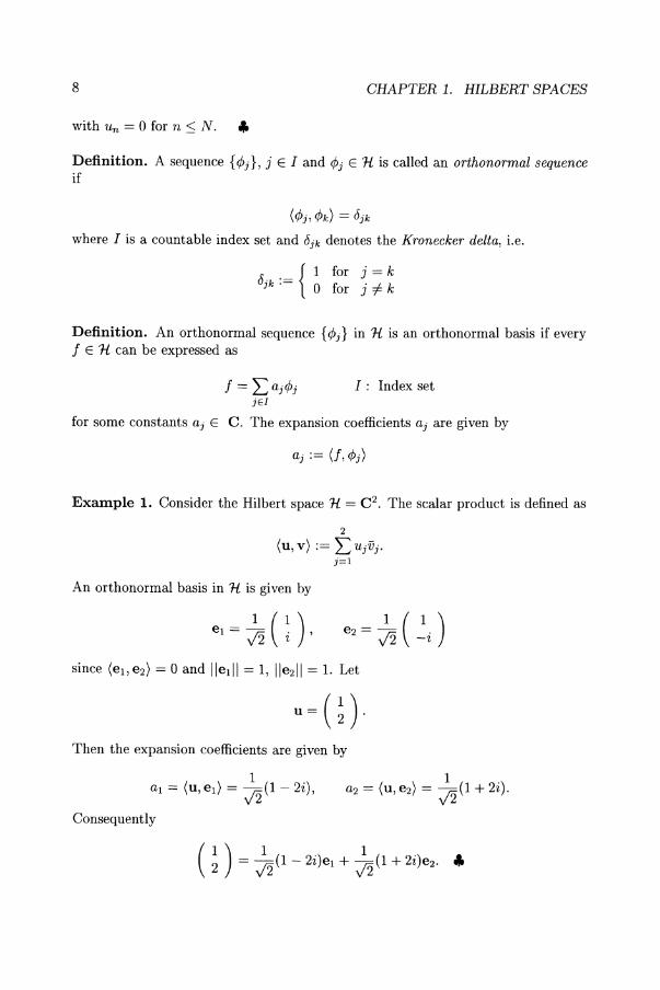
Definition. A sequence {¢j}, j E I and ¢j E 1-£ is called an orthonormal sequence if
(¢j, ¢k) = Jjk
where I is a countable index set and Jjk denotes the Kronecker delta, i.e.
{ I for j = k Jjk := 0 for j =1= k
Definition. An orthonormal sequence {¢j} in 1-£ is an orthonormal basis if every f E 1-£ can be expressed as
f = Laj¢j I: Index set jEI
for some constants aj E C. The expansion coefficients aj are given by
Example 1. Consider the Hilbert space 1-£ = C 2• The scalar product is defined as
2
(u, v) := L UjVj. j=l
An orthonormal basis in 1-£ is given by
Then the expansion coefficients are given by
a1 = (u, e1) = ~(1 - 2i),
Consequently
9
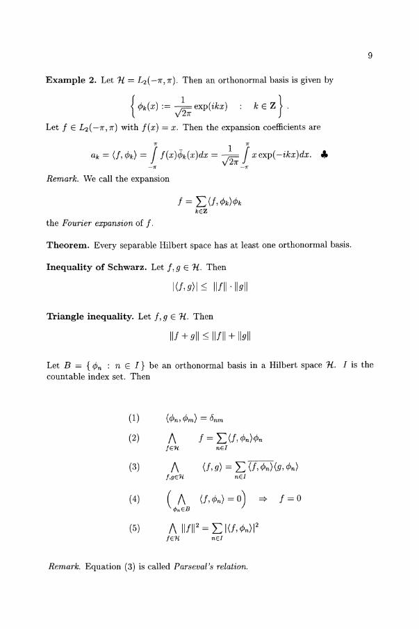
Example 2. Let 1£ = L 2 ( -7r, 7[-). Then an orthonormal basis is given by
{ I. cPk(X) := V2ir exp(zkx)
Let f E L 2 ( -7r, 7r) with f(x) = x. Then the expansion coefficients are
1T _ 1 1T
ak = (I, cPk) = J f(X)cPk(X)dx = V2ir J xexp( -ikx)dx. " -~ -~
Remark. We call the expansion
the Fourier expansion of f.
Theorem. Every separable Hilbert space has at least one orthonormal basis.
Inequality of Schwarz. Let f, 9 E 1£. Then
1(1, g)l::; IIfll·llgll
Triangle inequality. Let f, 9 E 1£. Then
Ilf + gil::; Ilfll + Ilgll
Let B = {cPn : n E I} be an orthonormal basis in a Hilbert space 1£. I is the countable index set. Then
(1) (cPn, cPm) = 8nm
(2) 1\ f = L (I, cPn)cPn IE1/. nEI
(3) 1\ (I, g) = L (I, cPn)(g,cPn) l,gE1/. nEI
(4) C~B (I,cPn) = 0) ~ f=O
(5) 1\ IIfll2 = L 1(1, cPnW IE1/. nEI
Remark. Equation (3) is called Parseval's relation.
10
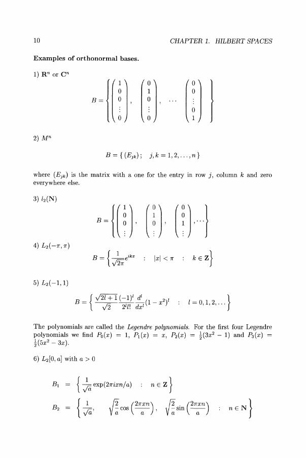
Examples of orthonormal bases.
B=
1 o o
o
o 1 o
o
CHAPTER 1. HILBERT SPACES
o o
o 1
B = { (Ejk ); j, k = 1,2, ... , n}
where (Ejk ) is the matrix with a one for the entry in row j, column k and zero everywhere else.
Ixl < 7r
l = 0,1,2, ... }
The polynomials are called the Legendre polynomials. For the first four Legendre polynomials we find Po(x) = 1, Pl(x) = X, P2(x) = ~(3X2 - 1) and P3(X) = !(5x2 - 3x).
6) L2 [0, a] with a > 0
{ Ja exp(27rixn/a)
vr (27rXn) -cos -- , a a vr . (27rXn) -sm --
a a
{II . 7rxn -sm-a a
f2 (7rxn) v~cos ~
B = { (27r~n/2 exp(ik . x)
where IXj I < 7r and kj E Z.
8) L2([0, a] x [0, a] x [0, aD
B = { _1_ei27rn.x/a a3/ 2
where a > ° and nj E Z.
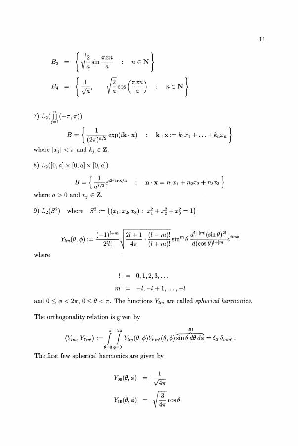
(_l)l+m 2l+1 (l-m)!. dl+1ml (sinO)21. y, (0 c/J) --. smmO e,m</> 1m, := 21l! 47r (l+m)! d(cosO)I+lml
where
0,1,2,3, ...
m -l, -l + 1, ... ,+l
and 0 :::; c/J < 27r, 0 :::; 0 < 7r. The functions Yim are called spherical harmonics.
The orthogonality relation is given by
7r 27r dO
(Yim, Yi'm'):= ! ! Yim(O, c/J)Yi'm' (0, c/J) ~in 0 dO d~ = 611'6mm, . 6=0</>=0
The first few spherical harmonics are given by
YOo(O,c/J) 1
= v'47f
Yio(O, c/J) I"fCOSO
11
12 CHAPTER 1. HILBERT SPACES
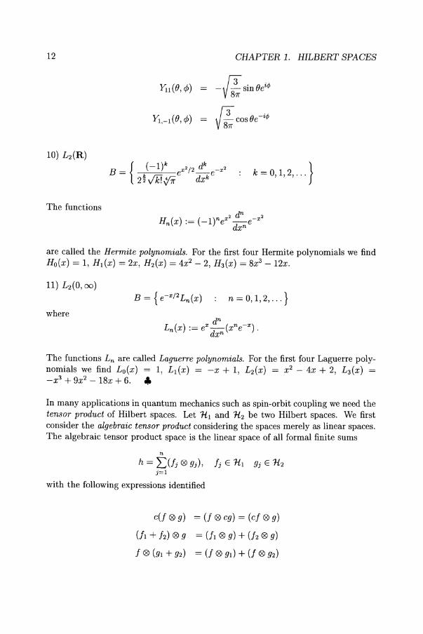
k =0,1,2, ... }
The functions
are called the Hermite polynomials. For the first four Hermite polynomials we find Ho(x) = 1, Hl(X) = 2x, H2(X) = 4X2 - 2, H3(X) = 8X3 - 12x.
n = 0,1,2, ... }
where
The functions Ln are called Lag'u,erre polynomials. For the first four Laguerre polynomials we find Lo(x) 1, Ll(X) = -x + 1, L2(X) = x2 - 4x + 2, L3(X) = -x3 + 9X2 - 18x + 6. ..
In many applications in quantum mechanics such as spin-orbit coupling we need the tensor product of Hilbert spaces. Let 1il and 1i2 be two Hilbert spaces. We first consider the algebraic tensor product considering the spaces merely as linear spaces. The algebraic tensor product space is the linear space of all formal finite sums
n h = 'L,(fJ ® gj), fJ E 1il gj E 1i2
j=1
with the following expressions identified
c(f ® g) = (f ® cg) = (cf ® g)
(II + h) ® 9 = (II ® g) + (12 ® g)
f ® (gl + g2) = (f ® gd + (f ® g2)
13
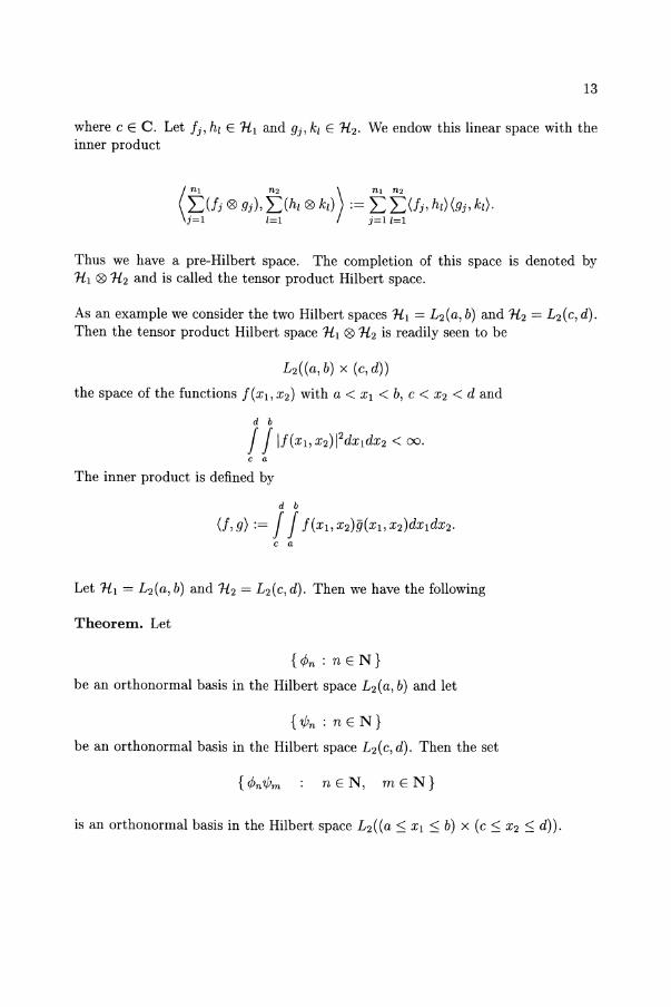
where c E C. Let Ii, hi E HI and gj, kl E H 2 . We endow this linear space with the inner product
Thus we have a pre-Hilbert space. The completion of this space is denoted by HI ®H2 and is called the tensor product Hilbert space.
As an example we consider the two Hilbert spaces HI = L2(a, b) and H2 = L2(c, d). Then the tensor product Hilbert space HI ®H2 is readily seen to be
L2 ((a, b) x (c, d))
the space of the functions f(xI, X2) with a < Xl < b, c < X2 < d and
d b
J J If(XI, X2W dx ldx2 < 00.
c a
The inner product is defined by
d b
(1, g) := J J f(XI, X2)g(XI, X2) dx ldx2. c a
Let HI = L2(a, b) and H2 = L2(c, d). Then we have the following
Theorem. Let
{<Pn : n E N}
be an orthonormal basis in the Hilbert space L2 (a, b) and let
{'l/Jn : n EN}
be an orthonormal basis in the Hilbert space L2 (c, d). Then the set
nEN, mEN}
is an orthonormal basis in the Hilbert space L2 (( a :::; Xl :::; b) x (c :::; X2 :::; d)).
14 CHAPTER 1. HILBERT SPACES
It is easy to verify by integration that the set is an orthonormal set over the rectangle. To prove completeness it suffices to show that every continuous function f(Xl, X2) with
d b
II f(Xl, X2) dXldx2 < 00
c a
whose Fourier coefficients with respect to the set are all zero, vanishes identically over the rectangle.
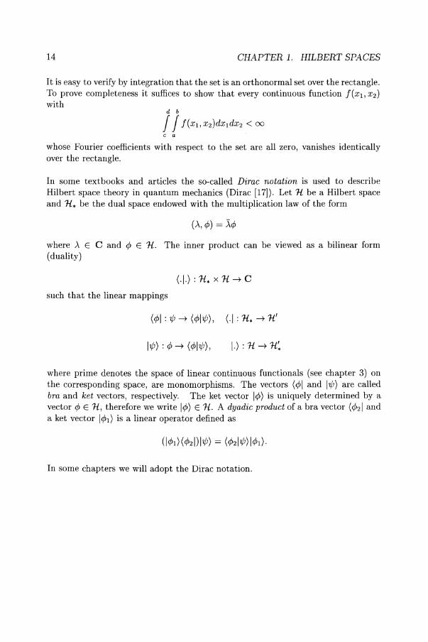
In some textbooks and articles the so-called Dirac notation is used to describe Hilbert space theory in quantum mechanics (Dirac [17]). Let 1£ be a Hilbert space and 1£. be the dual space endowed with the multiplication law of the form
(,x,¢) =)..¢
where ,X E C and ¢ E 1£. The inner product can be viewed as a bilinear form (duality)
(.1.) : 1£. x 1£-+ C
such that the linear mappings
(¢I : 'I/J -+ (¢I'I/J), (·1: 1£. -+ 1£'
I'I/J) : ¢ -+ (¢I'I/J), I·) : 1£-+ 1£:
where prime denotes the space of linear continuous functionals (see chapter 3) on the corresponding space, are monomorphisms. The vectors (¢I and I'I/J) are called bra and ket vectors, respectively. The ket vector I¢) is uniquely determined by a vector ¢ E 1£, therefore we write I¢) E 1£. A dyadic product of a bra vector (¢21 and a ket vector I¢l) is a linear operator defined as
In some chapters we will adopt the Dirac notation.
15
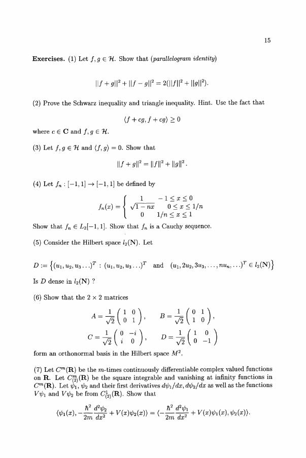
Exercises. (1) Let i, 9 E 1i. Show that (parallelogram identity)
(2) Prove the Schwarz inequality and triangle inequality. Hint. Use the fact that
(j + cg, i + cg) ;::: 0
where c E C and i, 9 E 1{.
(3) Let i, 9 E 1{ and (j, g) = O. Show that
(4) Let in : [-1, 1J -+ [-1, 1J be defined by
{I -l<x<O
in(x) = J1 - nx 0 S x S lin Olin S x S 1
Show that in E L2 [-1, 1 J. Show that in is a Cauchy sequence.
(5) Consider the Hilbert space l2(N). Let
D:={(Ul,U2,U3 ... f: (Ul,U2,U3 ... )T and (UI,2U2,3u3, ... ,nun, ... fEl2(N)}
Is D dense in l2 (N) ?
(6) Show that the 2 x 2 matrices
1 (1 0) A=J2 01'
1 (0 -i) C=J2 i 0 '
B=~(~ ~),
D = ~ (~ ~1) form an orthonormal basis in the Hilbert space M2.
(7) Let Cm(R) be the m-times continuously differentiable complex valued functions on R. Let C~)(R) be the square integrable and vanishing at infinity functions in Cm(R). Let 'ljJl, 'ljJ2 and their first derivatives d'ljJddx, d'ljJ2ldx as well as the functions V'ljJl and V'ljJ2 be from C(2)(R). Show that
h2 d2'ljJ h2 d2 'ljJ ('ljJl(X), - 2m dX22 + V(X)'ljJ2(X)) = (- 2m dX21 + V(X)'ljJl(X), 'ljJ2(X)).
16 CHAPTER 1. HILBERT SPACES
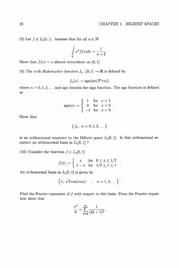
(8) Let f E L2 [O, 1]. Assume that for all n EN
1 1 f xnf(x)dx = n+2· o
Show that f(x) = x almost everywhere on [0,1].
(9) The n-th Rademacher function fn : [0,1] -+ R is defined by
fn(x) := sgn(sin(2n 7rx))
where n = 0,1,2, ... and sgn denotes the sign function. The sgn function is defined as
Show that
{I for x> 1
sgn(x) := ° for x = ° -1 for x < °
{ fn : n = 0, 1,2, ... }
is an orthonormal sequence in the Hilbert space L2 [0, 1]. Is this orthonormal sequence an orthonormal basis in L 2 [0, 1] ?
(10) Consider the function f E L 2 [0, 1]
{X for 0::; x ::; 1/2
f(x):= 1 - x for 1/2::; x ::; 1
An orthonormal basis in L2 [0, 1] is given by
{I, v'2cos(7rnx) n = 1,2, ... } .
Find the Fourier expansion of f with respect to this basis. From the Fourier expansion show that
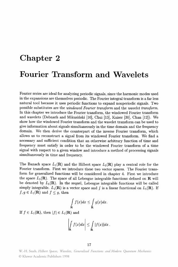
Chapter 2
Fourier Transform and Wavelets
Fourier series are ideal for analyzing periodic signals, since the harmonic modes used in the expansions are themselves periodic. The Fourier integral transform is a far less natural tool because it uses periodic functions to expand non periodic signals. Two possible substitutes are the windowed Fourier transform and the wavelet transform. In this chapter we introduce the Fourier transform, the windowed Fourier transform and wavelets (Debnath and Mikusinski [16], Chui [13], Kaiser [30], Chan [12]). We show how the windowed Fourier transform and the wavelet transform can be used to give information about signals simultaneously in the time domain and the frequency domain. We then derive the counterpart of the inverse Fourier transform, which allows us to reconstruct a signal from its windowed Fourier transform. We find a necessary and sufficient condition that an otherwise arbitrary function of time and frequency must satisfy in order to be the windowed Fourier transform of a time signal with respect to a given window and introduce a method of processing signals simultaneously in time and frequency.
The Banach space L 1(R) and the Hilbert space L2 (R) playa central role for the Fourier transform. First we introduce these two vector spaces. The Fourier transform for generalized functions will be considered in chapter 4. First we introduce the space L1(R). The space of all Lebesgue integrable functions defined on R will be denoted by L1(R). In the sequel, Lebesgue integrable functions will be called simply integrable. L1 (R) is a vector space and J is a linear functional on L1 (R). If f,g E L1(R) and f:S g, then
f f(x)dx :S f g(x)dx. R R
If f E Ll(R), then If I E L1(R) and
Ii f(X)dXI :S ilf(x)ldx.
17
W.-H. Steeb, Hilbert Spaces, Wavelets, Generalised Functions and Modern Quantum Mechanics© Kluwer Academic Publishers 1998
18 CHAPTER 2. FOURIER TRANSFORM AND WAVELETS
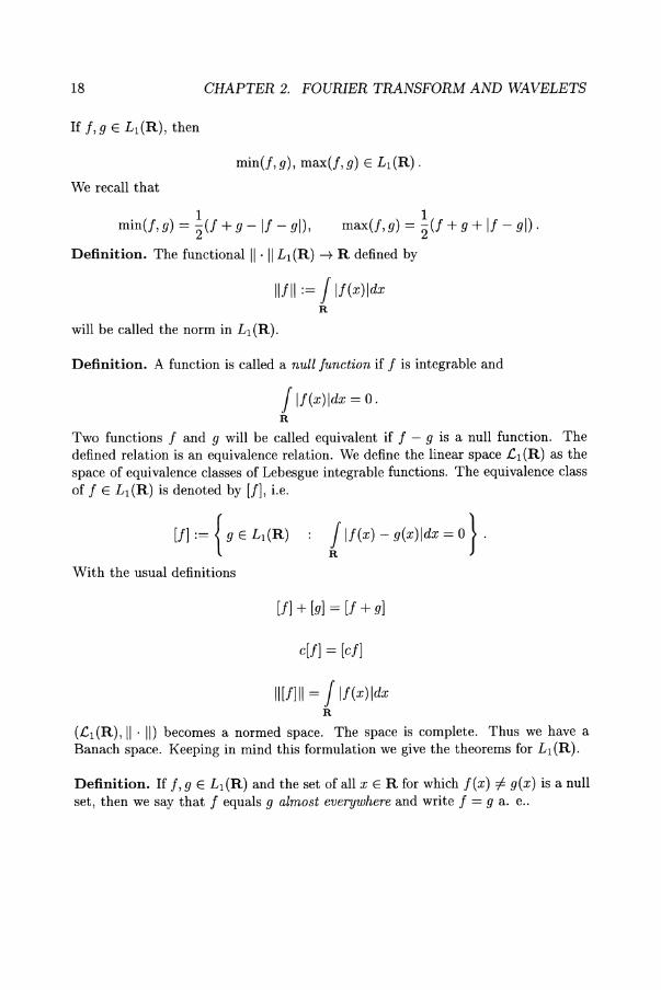
If f,g E L1(R), then
min(J, g), max(f, g) E L1(R).
We recall that
min(f, g) = ~(J + 9 - If - gl), 1
max(J, g) = 2(J + 9 + If - gl).
Definition. The functional II . II L1 (R) --+ R defined by
IIfll := J If(x)ldx R
will be called the norm in L1 (R).
Definition. A function is called a null function if f is integrable and
J If(x)ldx = O. R
Two functions f and 9 will be called equivalent if f - 9 is a null function. The defined relation is an equivalence relation. We define the linear space £l(R) as the space of equivalence classes of Lebesgue integrable functions. The equivalence class of f E L1 (R) is denoted by [f]' i.e.
If] := {g E L1(R)
With the usual definitions
Ilf (x) - g(x)ldx = 0 } .
If] + [g] = If + g]
clf] = [ef]
II [I] II = J If(x)ldx R
(£1(R), II . II) becomes a normed space. The space is complete. Thus we have a Banach space. Keeping in mind this formulation we give the theorems for L1(R).
Definition. If f, 9 E L 1(R) and the set of all x E R for which f(x) =f. g(x) is a null set, then we say that f equals 9 almost everywhere and write f = 9 a. e ..
19
Definition. If the integral
J f(x - y)g(y)dy R
exists for all x E R, or at least almost everywhere, then it defines a function which is called the convolution of f and g, denoted by f * g.
Theorem. If f, g E Ll (R), then the function f (x - y) g (y) is integrable for almost all x E R. Moreover, the convolution
(J*g)(x):= J f(x-y)g(y)dy
is an integrable function and we have
J If * gldx s J If(x)ldx J Ig(x)ldx. R R R
For the proof we refer to Debnath and Mikusinski [16].
If f, g E Ll(R), then f * g = g * f.
We introduce the Fourier transform in L 2 (R) and discuss its basic properties. The definition of the transform in L2 (R) is not trivial. The integral
00 J eikx f(x)dx -00
cannot be used as a definition of the Fourier transform in L2 (R) because not all functions in L2 (R) are integrable. It is however possible to extend the Fourier transform from Ll (R) n L2(R) onto L2(R). We discuss properties of the Fourier transform in Ll (R) and then study properties of its extension. Let f be an integrable function on R. Consider the integral
00 J eikxf(x)dx, kER. -00
Since the function g(x) = eikx is continuous and bounded, the product eikx f(x) is a locally integrable function for any k E R. Moreover, since
for all k, x E R we have
and thus the integral exists for all k E R.
20 CHAPTER 2. FOURIER TRANSFORM AND WAVELETS
Definition. Let f E L1 (R). The function j defined by
00 j(k):= f eikxf(x)dx
-00
is called the Fourier transform of fin L1(R).
Instead of j the notation F{J(x)} is also used. The latter is especially convenient if instead of a letter f or 9 we want to use an expression describing a function, for example F{e-X2 }.
Example. Let a > o. Then
Example.
F{e-X2 } = -Jffe-k2 / 4 . ..
The following theorem is an immediate consequence of the definition.
Theorem. Let f, g, E L1 (R) and a E C. Then
F(J + g) = F(g) + F(g) and F(aJ) = aF(J).
Theorem. The Fourier transform of an integrable function is a continuous function.
The integral Coo' If(x)ldx defines a norm in L1(R). This norm will be denoted by II· lit, Le.,
00
IIfllt = f If(x)ldx, for f E L1(R). -00
Theorem. If ft, 12, ... E L1 (R) and IIfllt --t 0 as n --t 00 then the sequence {j} converges to j uniformly on R.
Theorem. If f E L1(R), then
lim Ij(k)1 = O. Ikl-400
Note that the space Co(R) of all continuous functions on R which vanish at infinity (Le., limlxl-4oo f(x) = 0), is a normed space with respect to the norm defined by
IIfll := sup If(x)l· xER
The theorems show that the Fourier transform is a continuous linear operator from L1 (R) int Co(R).
Theorem. Let f E L1(R). Then
(a) F{f(xn = F{J(-xn.
(b) F{f(x - yn = F{f(xne-iky .
(c) F{J(axn = (l/a)F{J(x/an,
21
a> O.
Theorem. If f is a continuous piecewise differentiable function, f, I' E L1(R), and limlxl-+oo f(x) = 0, then
F{f'} = -ikF{J}.
To prove this theorem we apply integration by parts.
Corollary. If f is a continuous piecewise n-times differentiable function with f, 1', ... , f(n) E L1(R), and limlxl-+oo f(k)x = 0 for k = 0, ... , n -1, then
Theorem. (Convolution Theorem). Let f, 9 E L1 (R). Then
F{f * g} = F{J}F{g}.
We now discuss the extension of the Fourier transform onto L2 (R). In the following II· 112 denotes the norm in L2(R), i.e.,
Theorem. Let f be a continuous function on R vanishing outside a bounded interval. Then j E L2 (R) and
The space of all continuous functions on R with compact support is dense in L2(R). The theorem shows that the Fourier transform is a continous mapping from that space into L2(R). Since the mapping is linear, it has a unique extension to a linear mapping from L2 (R) into itself. This extension will be called the Fourier transform on L2(R).
Definition. (Fourier 'fransform in L2(R)). Let f E L2 (R) and let {IPn} be a sequence of continuous functions with compact support convergent to f in L2(R), i.e., IIf - IPnl12 -* O. The Fourier transform of f is defined by
j = lim rpn n-+oo
22 CHAPTER 2. FOURIER TRANSFORM AND WAVELETS
where the limit is taken with respect to the norm in L2(R).
The theorem guarantees that the limit exists and is independent of a particular sequence approximating f. The convergence in L2(R) does not imply pointwise convergence and therefore the Fourier transform of a square integrable function is not defined at a point, unlike the Fourier transform of an integrable function. The Fourier transform of a square integrable function is defined almost everywhere. We should say that the function defined above belongs to the equivalence class of square integrable functions. In spite of this difference, we use the same symbol to denote both transforms. It will not cause any misunderstanding.
Theorem. Let f E L2(R). Then
n
j(k) = lim J eikxf(x)dx n ..... oo
-n
where the convergence is with respect to the norm in L2(R).
Proof. For n = 1,2,3, ... , define
{ f(x) if Ixl < n fn(x) = 0 if Ixl 2 n.
Then Ilf - fnl12 --t 0, and thus Ilj - jnl12 --t 0 as n --t 00.
Theorem. (Inversion of Fourier Transforms in L2(R)). Let f E L2(R). Then
1 n . A
f(x) = lim - J e-zkx f(k)dk n ..... oo 27r
-n
where the convergence is with respect to the norm in L2(R).
Corollary. If f E L1(R) n L2 (R), then the equality
00
f(x) = ~ J e-ikx j(k)dk 27r
-00
holds almost everywhere in R.
The transform defined above is called the inverse Fourier transform.
Theorem. If f, 9 E L2 (R), then
00 00
27r f f(x)g(x)dx = f j(k)g(k)dk. -00 -00
23
Proof. The polarization identity
1 (I, g) = 4(lf + gl2 - If - gl2 + ilf + igl2 - ilf - igl 2)
implies that every isometry preserves the inner product. Since the Fourier transform is an isometry on L2(R), we have 27r(l, g) = (/, g).
The following theorem summarizes the results of this section. It is known as the Plancherel Theorem.
Theorem. For every f E L2(R) there exist / E L2(R) such that
(a) If f E L1(R) n L2(R), then /(k) = f~oo eikx f(x)dx.
(b) lIi(k) - f~n eikx f(x)dxIl2 --+ 0 and
Ilf(x) -1/27r f~ne-ikXi(k)dkI12 --+ 0 as n --+ 00.
(c) 27rllfll~ = II/II~·
(d) The mapping f --+ i is a Hilbert space isomorphism of L2 (R) onto L2 (R).
For the proof we refer to Debnath and Mukusinski [16].
Theorem. The Fourier transform is an unitary operator on L2(R), i.e. F-1 = F*.
The Fourier transform can be defined for functions in L1 (RN) by
/(k) = J eik.x f(x)dx RN
where
and
k . x = k1X1 + ... + kNxN.
The theory of the Fourier transform in L1(RN) is similar to the one dimensional case. Moreover, the extension to L2(RN) is possible and it has similar properties, including the Inversion Theorem and the Plancherel Theorem. The inverse Fourier transform is given by
f(x) = (2~)n J e-ik.x /(k)dk. RN
24 CHAPTER 2. FOURIER TRANSFORM AND WAVELETS
Next we introduce the windowed Fourier transform. Let g(u) be a function that vanishes outside the interval -T ~ u ~ 0, i.e., such that supp 9 C [-T,O]. The function g(u) will be a weight function, or window, which will be used to "localize" signals in time. We allow 9 to be complex-valued, although in many applications it may be real. We assume in the following only that 9 E L2(R). For every t E R, define
ft(u) := g(u - t)f(u)
where g(u - t) == g(u - t). Then
suppft C [t - T, t]
and we think of ft as a localized version of f that depends only on the values f (u) for t - T ~ u ~ t. If 9 is continuous, then the values ft(u) with u ~ t - T and u ~ t are small. This means that the above localization is smooth rather than abrupt. We now define the windowed Fourier transform of f as the Fourier transform of ft
00 00
ft(w) = f duexp( -27l'iwu)ft(u) = f duexp(-27l'iwu)g(u - t)f(u). -00 -00
Thus ft(w) depends on f(u) only for t - T ~ u ~ t and (if 9 is continuous) gives little weight to the values of f near the endpoints. In order for the windowed Fourier transform to make sense, as well as for the reconstruction formula to be valid, it will only be necessary to assume that g(u) is square-integrable, i.e. 9 E L2(R). When g(u) == 1 (so 9 fj. L2(R)), the windowed Fourier transform reduces to the ordinary Fourier transform. In the following we merely assume that 9 E L2(R). If we define
gw,t(u) := e27riwug(u - t)
we obtain
ligw,tli = Ilgll·
Consequently gw,t also belongs to L2(R), and the windowed Fourier transform can be expressed as the innner product of f with gw,t
which makes sense if both functions are in L2 (R) .
Next we introduce wavelets. We recall that the scalar product in L2(R) is defined as
00
(J, g):= f f(x)g(x)dx. -00
Thus the induced norm is given by
25
where f,g E L2(R). Let f E L2(R). We consider f(2 j - k). Observe that the function
f(2 j x - k)
is obtained from the function f(x) by a binary dilation (i.e. dilation by 2j ) and a dyadic translation (of k/2 j ). For any j, k E Z, we have
Hence, if a function 'IjJ E L2 (R) has unit length, then all of the functions 'ljJj,k, defined by
'ljJj,k(X) := 2j/2'IjJ(2 jx - k),
also have unit length; that is
j,k E Z
j,k E Z.
Definition. A function 'IjJ E L2 (R) is called an orthogonal wavelet, if the family {'IjJj,d, as defined in
'ljJj,k := 2j/2'IjJ(2jx - k),
is an orthonormal basis of L2(R); that is,
j,k E Z
j,k,l,m E Z
and every f E L 2 (R) can be written as
00
f(x) = L Cj,k'IjJj,k(X) j,k=-oo
where the convergence of the series is in L2 (R), namely:
We are interested in wavelet functions 'IjJ whose binary dilations and dyadic translations are enough to represent all the functions in L2(R).
Example. The simplest example of an orthogonal wavelet is the Haar function 'ljJH defined by
{I for
'ljJH(X) := 0-1 for otherwise.
O~X<! !~x<l
26 CHAPTER 2. FOURIER TRANSFORM AND WAVELETS
Then
'lj!mn(X) := Tm/2'lj!(Tmx - n)
where m, n E Z. Thus 'lj!mn is given by
{I for
'lj!mn(x) = -1 for o otherwise
2m n:::; x < 2m n + 2m - 1
2m n + 2m - 1 :::; x < 2m n + 2m
Example. Another example is the Littlewood-Paley orthonormal basis of wavelets. The mother wavelet of this set is
L(x) := ~(sin(27f) - sin(7fX)) . 7fX
Using the definition
Lmn(x) := Tm/2 L(2-mx - n)
we generate an orthonormal set in L2(R). ..
The series representation of f 00
f(x) = L Cj,k'lj!j,k(X) j,k=-oo
is called a wavelet series. Analogous to the notion of Fourier coefficients, the wavelet coefficients Cj,k are given by
Cj,k = (f, 'lj!j,k)'
If we define an integral transform W.p on L 2 (R) by
1 00 (x - b) (W.pf)(b, a) := lal-2 f f(x)'lj! -a- dx, -00
then the wavelet coefficients can be written as
The linear transformation W.p is called the integral wavelet transform relative to the basic wavelet 'lj!. Hence, the (j, k)th wavelet coefficient of f is given by the integral wavelet transformation of f evaluated at the dyadic position
with binary dilation
27
where the same wavelet 'l/J is used to generate the wavelet series and to define the integral wavelet transform.
The integral wavelet transform greatly enhances the value of the (integral) Fourier transform :F defined above. Next we discuss inversion formulas and duals. The function f has to be reconstructed from the values of (W",f)(b, a). Any formula that expresses every f E L2(R) in terms of (W",f)(b, a) will be called an inverse formula, and the (kernel) function 1j; to be used in this formula will be called a dual of the basic wavelet 'l/J. Hence, in practice 'l/J can be used as a basic wavelet, only if an inversion formula exists. We consider four different situations, that need to be considered in the order of restrictiveness of the domain of information of W",f. For the details we refer to the literature [13].
1) Finding f from (W",f)(b, a) with a, bE R. In order to find f from W",f, we need to know the constant
c",:= l'~t?'2 dw < 00 -00
where ~ is the Fourier transform of'l/J. The finiteness of this constant restricts the class of L2(R) functions 'l/J that can be used as basic wavelets in the definition of the integral wavelet transform. In particular, if'l/J must also be a window function, then'l/J is necessarily in LI(R), i.e.
00
J 1'l/J(x)ldx < 00 -00
Thus the function ~ is a continuous function in R. It follows that ~ must vanish at the origin. Thus
00 J 'l/J(x)dx = O. -00
So, the graph of a basic wavelet 'l/J is a small wave. With the constant C"', we have the following reconstruction formula
f(x) = ~ Joo Joo {(W",f)(b,a)} {~'l/J (x - b)} dadb, C'" -00 -00 lal 2 a a2
One cannot expect uniqueness of this dual.
2) Finding f from (W",f)(b, a) with b E R and a > O. In time-frequency analysis we use a positive constant multiple of a-I to represent frequency. Hence, since only positive frequency is of interest, we need a reconstruction formula where the integration is over R x (0,00) instead of R2. Therefore, we must now consider even
28 CHAPTER 2. FOURIER TRANSFORM AND WAVELETS
a smaller class of basic wavelets 'I/J, namely the function 'I/J must satisfy
/00 1?,b(w)12 dw = /00 l?,b( -W)12 dw = ~C.p < 00.
w w 2 o 0
For any 'I/J satisfying this equation we have the following reconstruction formula
With the exception of a factor of 2, this formula is the same as the reconstruction formula for the case a, bE R. The basic wavelet 'I/J for the case 2) is more restrictive. We call the complex conjugate 1f of'I/J a dual of the basic wavelet 'I/J for the case 1). There is no reason to expect a unique dual.
3) Finding f from (W.pj)(b, a) with b E R, a = fr where j E Z. The reconstruction formula by using this dual may be stated as follows [13]
00 00
f(x) =.2:: / {2i/2 (W.pf)(b, Ti)}{2i'I/J*(2i(x - b))}db, 3==-00_00
Since basic wavelets 'I/J for this situation have both theoretical and practical value, they are given the following special name.
Definition. A function 'I/J E L2(R) is called a dyadic wavelet if it satisfies the stability condition
00
A:S; 2:: 1?,b(Ti w)12:s; B i==-oo
for almost all w E R for some constants A and B with 0 < A :s; B < 00.
4) For the case of the reconstruction of f from (W.pj)(b, a) where b = k/2i, a = 1/2i
with j, k E Z we refer to the literature (Chui [13]).
Exercises. (1) Let f E L 1(R) n L2(R). Show that
F(F[J(x)]) = 27rf(-x).
(2) Let fELl (R) and assume that f is continuously differentiable and
df dx E Ll(R).
Show that
F [:~] = -ikF[J] .
(3) Let 9, fELl (R) n L2 (R) and g and j be the Fourier transform. Show that
1 ' (9,1) = 27r (g, 1) .
(4) Show that the inverse Fourier transform of the symmetric function
j(W)={l for.7r<lwl<27r o otherwise
is given by
f( ) - sin(7rt/2) (37rt) t - 7rt/2 cos 2 .
(5) Find functions f such that
(6) Let
Show that
where
00
f(w) = I f(t)eiwtdt. -00
00
S(w) = I S(t)eiwtdt, 1/00, "t S(t) = - S(w)e-'W dw.
27r -00
00
1 .0. t . .0. >w- 2
J t 2 IS(t)1 2dt
-00
00
J w2 IS(w)j2dw .0.; := _-00=00--- .0.~ :=--00--::-00:----
J IS(t)l2dt J IS(w)l2dw -00 -00
29
30 CHAPTER 2. FOURIER TRANSFORM AND WAVELETS
(7) Let
1 (t2 ) J(t):= ftC exp --2 . y27fat 2at
Show that
. ( W2) J(w) = exp - 2a~ .
(8) Let
J(t) = exp(27fiat)
where a E R. Obviously, J(t) ~ L2(R). Show that windowed Fourier transform of J with respect to the Gaussian window
get) = exp( _7ft2)
is well defined. Find the windowed Fourier transfrom.
(9) Let
'Ij;(t) = ~(t2 _ 1)e-t2 / 2. 27f
This function is called the Mexican hat function. Consider
where m, n E Z. Calculate
Chapter 3
Linear Operators in Hilbert Spaces
A linear operator, A, in a Hilbert space, 'N, is a linear transformation of a linear manifold, V(A) (c 1-£), into 1-£. The manifold V(A) is termed the domain of definition, or simply the domain, of A. Throughout this chapter we consider linear operators.
Definition. The linear operator A is termed bounded if the set of numbers, IIAfll, is bounded as f runs through the normalized vectors in V(A). In this case, we define IIAII, the norm of A, to be the supremum, i.e. the least upper bound, of IIAfll, as f runs through these normalized vectors, i.e.
IIAII := sup IIAfll· 11/11=1
Example. Let 1-£ = en. Then all n x n matrices over e are bounded linear operators. If In is the n x n identity matrix we have II In II = 1. ..
Example. Consider the Hilbert space L2 (0, a) with a > 0. Let Af(x) := xf(x). Then V(A) = L2 (0, a) and IIAII = a. ..
It follows from this definition that
IIAfl1 ~ IIAlillfll for all vectors f in V(A).
If A is bounded, we may take V(A) to be 'N, since, even if this domain is originally defined to be a proper subset of 'N, we can always extend it to the whole of this space as follows. Since
IIAim - Ainll ~ IIAllllim - inll
31
W.-H. Steeb, Hilbert Spaces, Wavelets, Generalised Functions and Modern Quantum Mechanics© Kluwer Academic Publishers 1998
32 CHAPTER 3. LINEAR OPERATORS IN HILBERT SPACES
we conclude that the convergence of a sequence of vectors {fn} in D(A) implies that of {Afn}. Hence, we may extend the definition of A to D(A), the closure of D(A), by defining
A lim fn := lim Afn-n-+oo n--+oo
We may then extend A to the full Hilbert space 1l, by defining it to be zero on D(A).l, the orthogonal complement of D(A).
On the other hand, if A is unbounded, then in general, D(A) does not comprise the whole of 1l and cannot be extended to do so.
Example. Consider the differential operator d/ dx acting on the Hilbert space, 1l, of square-integrable functions of the real variable x. The domain of this operator consists of those functions f(x) for which both J If(x)1 2dx and J Idf(x)/dxI 2dx are both finite, and this set of functions does not comprise the whole of 1l. ...
Definition. Let A be a bounded operator in 1l. We define A*, the adjoint operator of A, by the formula
(J,A*g):= (Af,g) for all f,g E 1l.
Definition. The operator A is termed self-adjoint if A* = A or, equivalently, if
(J, Ag) = (Af, g) for all f, 9 E 1l.
Example. Let 1l = C 2 • Then
A = (~i ~) is a self-adjoint operator (hermitian matrix). ...
In the case where A is an unbounded operator in 1l we again define its adjoint, A * , by the same formula, except that f is confined to D(A) and 9 to the domain D(A*), which is specified as follows: 9 belongs to D(A*) if there is a vector gA in 1l such that
(J, gA) = (Af, g) for all f in D(A)
in which case gA = A*g. The operator A is termed self-adjoint ifD(A*) = D(A) and A* = A. The coincidence of D(A*) with D(A) is essential here. The domain of a self-adjoint operator is dense in 1l.
Remark. If merely (Af, g) = (J, Ag) for all f, 9 E D(A), and if D(A) is dense in 1l, i.e., if A c A*, then A is called hermitian (symmetric); D(A*) may be larger than D(A), in which case A* is a proper extension of A.
33
Definition. Let A be a linear operator with dense domain. Then its nullspace is defined by
N(A) := { u E 1l : Au = O}.
Definition. A self-adjoint operator A is termed positive if
(I, Ai) 20
for all vectors f in V(A).
Example. Let B be a bounded operator. We define A := B* B. Then A is a bounded self-adjoint operator and the operator A is positive. "
Remark. If B is unbounded, then B* B need not be self-adjoint.
Remark. An operator product AB is defined on a domain
V(AB) = { v E V(B) : Bv E V(A) }
and then
(AB)v := A(Bv).
Therefore V(A*A) may be smaller than V(A).
Next we summarize the algebraic properties of the operator norm. It follows from the definitions of the norm and the adjoint of a bounded operator, together with the triangular inequality that if A, B are bounded operators and c E C, then
IlcA11 IIA*AII
IIA+BII IIABII
IclllAIl IIAI12
< IIAII+IIBII < IIAIIIIBII·
Definition. Suppose that K is a subspace of 1l. Then since any vector f in 1i may be resolved into unequally defined components hand h.L in K and K 1-,
respectively, we may define a linear operator II by the formula IIf = h. This is termed the projection operator from 1l to K, or simply the projection operator or projector for the subspace K.
It follows from this definition and the orthogonality of hand fK.L that
34 CHAPTER 3. LINEAR OPERATORS IN HILBERT SPACES
and therefore that II is bounded. It also follows from the definition of II that
II2 = II = II" .
This formula is generally employed as a definition of a projection operator, II, since it implies that the set of elements {III} form a subspace of 11., as I runs through the vectors in 1-£.
Example. Let 1-£ = R2. Then
II = ~ (1 -1) 2 2 -1 1
are projection operators (projection matrices). We have II1II2 = O. ..
Example. In the case where K is a one-dimensional subspace, consisting of the scalar multiples of a normalized vector ¢, the projection operator II = II( ¢) is given by
II(¢)I = (¢, f)¢. ..
Definition. An operator, U, in a Hilbert space 11. is termed a unitary operator if
(UI, Ug) = (I, g)
for all vectors I, 9 in 11., and if U has an inverse U- 1, i.e. UU-1 = U-1U = I, where I is the identity operator, i.e. I I = I for all I E 11..
In other words, a unitary operator is an invertible one which preserves the form of the scalar product in 1-£. The above definition of unitarity is equivalent to the condition that
U·U = UU* = I i.e. U· = U-1 .
A unitary mapping of 11. onto a second Hilbert space 1-£' is an invertible transformation V, from 11. to 11.', such that
(I, g)1£ = (V I, V g)1£' .
Example. Let 11. = C 2 . Then
U = ( O. i) -z 0
is a unitary operator (unitary matrix). ..
Next we discuss operator convergence. Suppose that A and the sequence {An} are bounded linear operators in 1-£.
35
Definition. The sequence of operators An is said to converge uniformly, or in norm, to A as n -+ (Xl if
IIAn - All -+ 0 as n -+ (Xl •
Definition. The sequence of operators An is said to converge strongly to A if Anf tends strongly to Af for all vectors f in H.
Definition. The sequence of operators An is said to converge weakly to A if Anf tends weakly to Af for all vectors f in 1{.
Example. Consider the Hilbert space L2(R). Let An be the translation operator
(AnJ)(x) := f(x + 2n).
The operator An converges weakly to the zero operator. However, An does not converge strongly to anything, since if it did the limit would have to be zero, whereas, for any f, IIAnfl1 = Ilfll, which does not tend to zero. ..
From these definitions, it follows that norm convergence implies strong operator convergence, which in turn implies weak operator convergence. The converse statements are applicable only if H is finite dimensional, i.e. H = en.
Definition. A density matrix, p, is an operator in H of the form
where {II( ¢n) } are the projection operators for an orthonormal sequence {¢n} of vectors and { Wn } is a sequence of non-negative numbers whose sum is unity. Thus, a density matrix is bounded and positive.
Definition. The trace of a positive operator B is defined to be
tr(B) := ~(¢n' B¢n) nEI
where {¢n : n E I} is any orthonormal basis set. The value of tr(B), which is infinite for some operators, is independent of the choice of basis.
It follows from these definitions of density matrices and trace that a density matrix is a positive operator whose trace is equal to unity.
Definition. A one-parameter group of unitary transformations of H is a family {Utl of unitary operators in H, with t running through the real numbers, such that
Uo = I.
36 CHAPTER 3. LINEAR OPERATORS IN HILBERT SPACES
The group is said to be continuous if Ut converges strongly to I as t tends to zero; or equivalently, if Ut converges strongly to Uto as t tends to to, for any real to. In this case, Stone's theorem tells us that there is a unique self-adjoint operator, K, in 1l such that :t Uti = iKUtI = iUtK f for all f in V(K).
This equation is formally expressed as
and iK is termed the infinitesimal generator of the group {Ut }.
Example. Let
( 0 i) K = -i 0 .
Then
U = eiKt = (C?st -sint). .. t smt cost
Next we consider linear operators in tensor product space. Suppose that 111 and 112 are Hilbert spaces, and that 1£ is a third Hilbert space, defined in terms of 1ll and 112 as follows. We recall that for each pair of vectors h, 12 in 1ll' 1l2' respectively, there is a vector in 1l, denoted by h ® 12, such that
If Al and A2 are operators in HI and 1l2' respectively, we define the operator Al ®A2 in 1ll ® 112 by the formula
Al ® A2 is called the tensor product of Al and A2.
Similarly, we may define the tensor product 1£1 ® 1£2 ® ... ® 1ln as well as that, Al ® A2 ® ... ® An, of operators AI,"', An. In standard notation, one writes
n ® 1lj = 1ll ® 112 ® ... ® 1ln j=l
and n
® Aj = Al ® A2 ® ... ® An. j=l
37
Let us now discuss the spectrum of a linear operator. Let T be a linear operator whose domain V(T) and range R(T) both lie in the same complex linear topological space X. In our case X is a Hilbert space 1/.. We consider the linear operator
where A is a complex number and I the identity operator. The distribution of the values of A for which TA has an inverse and the properties of the inverse when it exists, are called the spectral theory for the operator T. We discuss the general theory of the inverse of TA (Yosida [69)).
Definition. If Ao is such that the range R(TAo) is dense in X and TAO has a continuous inverse (AoI - T)- 1, we say that Ao is in the resolvent set {!(T) of T, and we denote this inverse (AoI - T)-l by R(Aoj T) and call it the resolvent (at Ao) of T. All complex numbers A not in (!(T) form a set a(T) called the spectrum of T. The spectrum a(T) is decomposed into disjoint sets Pq(T), Gu(T) and Rq(T) with the following properties:
Pq(T) is the totality of complex numbers A for which TA does not have an inverse. Pu(T) is called the point spectrum of T. In other words the point spectrum Pu(T) is the set of eigenvalues of Tj that is
Pq(T) := {A E C : T I = AI for some nonzero I in X}.
Gu(T) is the totality of complex numbers A for which TA has a discontinuous inverse with domain dense in X. Gu(T) is called the continuous spectrum of T.
Ru(T) is the totality of complex numbers A for which TA has an inverse whose domain is not dense in X. Rq(T) is called the residual spectrum of T.
For these definitions and the linearity of the operator T we find the
Proposition. A necessary and sufficient condition for Ao E Pq(T) is that the equation
TI = >'01 has a solution I i 0 (J E X). In this case Ao is called an eigenvalue of T, and I the corresponding eigenvector. The null space N(>'oI - T) of TAO is called the eigenspace of T corresponding to the eigenvalue Ao of T. It consists of the vector 0 and the totality of eigenvectors corresponding to >'0' The dimension of the eigenspace corresponding to >'0 is called the multiplicity of the eigenvalue >'0.
Theorem. Let X be a complex Banach-space, and T a closed linear operator with its domain V(T) and range R(T) both in X. Then, for any >'0 E {!(T), the resolvent (AoI - T)-l is an everywhere defined continuous linear operator. For the proof we refer to Yosida [69].
38 CHAPTER 3. LINEAR OPERATORS IN HILBERT SPACES
Example 1. If the linear space X is of finite dimension, then any bounded linear operator T is represented by a matrix (tij). The eigenvalues of T are obtained as the roots of the algebraic equation, the so-called secular or characteristic equation of the matrix (tij):
where det(.) denotes the determinant of the matrix. •
Example 2. Consider the Hilbert space 1£ = L2(R). Let T be defined by
Tf(x) := xf(x)
that is,
V(T) = {f(x) : f(x) and xf(x) E L2 (R) }
and Tf(x) = xf(x) for f(x) E V(T). Then every real number AO is in Cu(T), i.e. T has a purely continuous spectrum consisting of the entire real axis. For the proof we refer to Yosida [69]. •
Example 3. Let X be the Hilbert space 12(N). Let T be defined by
Then ° is in the residual spectrum of T, since R(T) is not dense in l2(N). •
Example 4 Let H be a self-adjoint operator in a Hilbert space 1£. The spectrum a(H) lies on the real axis. The resolvent set (}(H) of H comprises all the complex numbers A with <;S(A) i= 0, and the resolvent R(A; H) is a bounded linear operator with the estimate
Moreover,
1 IIR(A; H) II :'S I <;S(A) I·
<;S((U - H)f, 1) = <;S(A)llfI12, f E V(H).
Example 5. Let U be a unitary operator. The spectrum lies on the unit circle IAI = 1; i.e. the interior and exterior of the unit circle are the resolvent set (}(U). The residual spectrum is empty. •
Example 6. Consider the linear bounded self-adjoint operator in a Hilbert space h(N)
A=
In other words
o 1 0 0 1 0 1 0 o 1 0 1
if i=j+l if i=j-l
otherwise
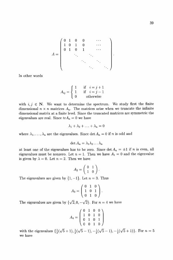
39
with i, j E N. We want to determine the spectrum. We study first the finite dimensional n x n matrices An. The matrices arise when we truncate the infinite dimensional matrix at a finite level. Since the truncated matrices are symmetric the eigenvalues are real. Since trAn = 0 we have
where A1> ... , An are the eigenvalues. Since det An = 0 if n is odd and
det An = A1A2 ... An
at least one of the eigenvalues has to be zero. Since det An = ±1 if n is even, all eigenvalues must be nonzero. Let n = 1. Then we have Ai = 0 and the eigenvalue is given by A = O. Let n = 2. Then we have
A2 = (~ ~). The eigenvalues are given by {I, -I}. Let n = 3. Thus
A3=(~ ~ ~). 010
The eigenvalues are given by {V2, 0, -V2}. For n = 4 we have
A4=(~ H lJ o 0 1 0
with the eigenvalues H(v15 + 1), Hv15 - 1), -Hv15 - 1), -Hv15 + I)}. For n = 5 we have
40 CHAPTER 3. LINEAR OPERATORS IN HILBERT SPACES
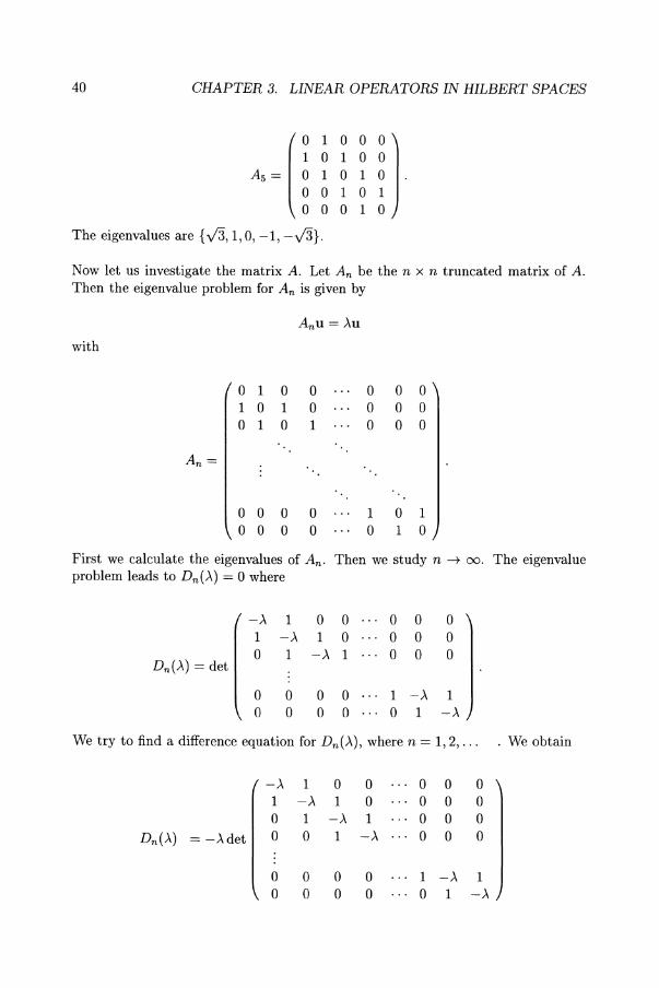
[0 1 0 0
n 1 0 1 0 As = 0 1 0 1
o 0 1 0 o 0 0 1
The eigenvalues are {V3, 1,0, -1, -V3}.
Now let us investigate the matrix A. Let An be the n x n truncated matrix of A. Then the eigenvalue problem for An is given by
Anu = AU
with
0 1 0 0 0 0 0 1 0 1 0 0 0 0 0 1 0 1 0 0 0
An=
0 0 0 0 1 0 1 0 0 0 0 0 1 0
First we calculate the eigenvalues of An. Then we study n ~ 00. The eigenvalue problem leads to Dn(A) = 0 where
-A 1 0 0 0 0 0 1 -A 1 0 0 0 0
Dn(A) = det 0 1 -A 1 0 0 0
0 0 0 0 1 -A 1 0 0 0 0 0 1 -A
We try to find a difference equation for Dn(A), where n = 1,2, ... . We obtain
-A 1 0 0 0 0 0 1 -A 1 0 0 0 0 0 1 -A 1 0 0 0
Dn{A) = -Adet 0 0 1 -A 0 0 0
0 0 0 0 1 -A 1 0 0 0 0 0 1 -A
41
1 1 0 0 0 0 0 0 -,\ 1 0 0 0 0 0 1 -,\ 1 0 0 0
-det
0 0 0 0 1 -,\ 1 0 0 0 0 0 1 -,\
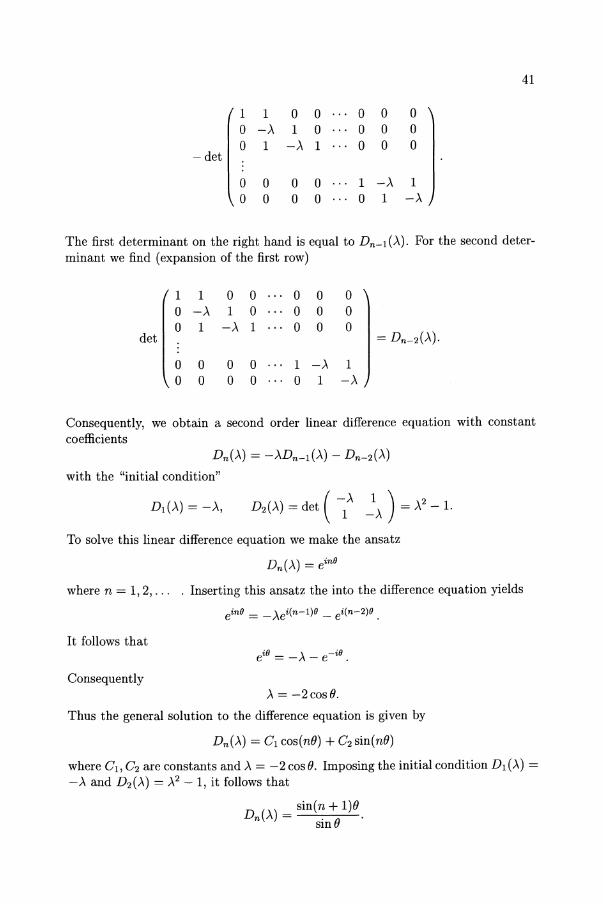
The first determinant on the right hand is equal to Dn - l ('\). For the second determinant we find (expansion of the first row)
1 1 0 0 0 0 0 0 -,\ 1 0 0 0 0 0 1 -,\ 1 0 0 0
det = Dn - 2 (,\).
0 0 0 0 1 -,\ 1 0 0 0 0 0 1 -,\
Consequently, we obtain a second order linear difference equation with constant coefficients
with the "initial condition"
( -,\ 1) 2 D2('\) = det 1 -,\ =,\ - 1.
To solve this linear difference equation we make the ansatz
Dn('\) = einB
where n = 1,2, . .. . Inserting this ansatz the into the difference equation yields
einB = _'\ei(n-l)B _ ei(n-2)B .
It follows that
Consequently ,\ = -2cosB.
Thus the general solution to the difference equation is given by
Dn('\) = Gl cos(nB) + G2 sin(nB)
where G l , G2 are constants and ,\ = -2 cos B. Imposing the initial condition Dl (,\) =
-,\ and D2('\) = ,\2 - 1, it follows that
Dn('\) = sin(~ + 1)0. smB
42 CHAPTER 3. LINEAR OPERATORS IN HILBERT SPACES
Since DnC)") = 0 we find
sin(~ + 1)0 = o. smO
The solutions to this equation are given by
O=~ n+1
with k = 1,2, ... ,n. Since A = -2 cos 0, we find the eigenvalues
Ak = -2 cos (~) n+1
with k = 1,2, ... , n. Consequently,
(i) IAkl < 2.
and Ak =j:. Ak' if k =j:. k'. If n -t 00, then
(ii) infinitely many Ak with IAkl ::; 2
and
(iii) Ak - Ak+1 -t 0 for n -t 00.
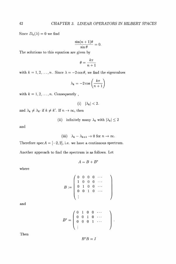
Therefore specA = [-2,2], i.e. we have a continuous spectrum.
Another approach to find the spectrum is as follows. Let
A = B+B*
where
0 0 0 0 1 0 0 0
B·- 0 1 0 0 0 0 1 0
and
B'~ C 1 0 0
) 0 1 0 0 0 1
Then B*B =1
43
where I is the infinite unit matrix. Notice that BB* =f=. I. We use the following notation
C f = >..j means
as n -+ 00. Now
B f = )..f =} B* B f = B* >..j =} f = )"B* f =} B* f = ~ f .
From B f = )..f it also follows that
IIBfll2 = (Bf,Bf) = (i,B*Bf) = (i,f) = Ilfll2.
On the other hand (Bf, Bf) = )..)..(i, f) = 1)..121IfI12 .
Since Ilfll > 0 we find that
Therefore
1 -Af = (B + B*)f = ().. + X)1 = ().. + )..)f = 2(cos-y)f·
This means 1\ II(A - 2(cos-y)I)fnll -+ 0
'1'ER
or
A ( :::~ ) ~ 2=~ ( :::~ ) E loo(N).
The linear space loo(N) is a Banach space B defined as
loo(N) := {x E l(N) : IIxll := sup Ixul < 00 } nEN
where l(N) is the linear space of infinite sequences x = (Xl, X2, .•• ), where Xj E C. However, the eigenvector is not an element of l2 (N). For the first two rows we have the identities
The norm is given by
sin 2-y
sin -y + sin 3-y
2 sin -y cos -y
2 cos -y sin 2-y
44 CHAPTER 3. LINEAR OPERATORS IN HILBERT SPACES
iiAii = sup iaioESpec A = max iaioESpec A = 2. ..
Example 7. The operator -d?,/dx2, with a suitably chosen domain in L2(R) has a purely continuous spectrum consisting of the nonnegative real axis. The negative real axis belongs to the resolvent set. ..
Example 8. The operator _~/dX2 +x2, with a suitably chosen domain in L2(R), has a pure point spectrum consisting of the positive odd integers, each of which is a simple eigenvalue. (see chapter 12) ..
Example 9. Let 11. = l2(N). Let A be the unitary operator that maps
onto
Au = (U2' U4, Ut, U6, U3,"" U2n+2, U2n-I," .)T. The point spectrum is empty and the continuous spectrum is the entire unit circle in the >. plane. ..
Example 10. In the Hilbert space 11. = l2(N U {O}), annihilation and creation operators denoted by band b* are defined as follows. They have a common domain
00
VI = V(b) = V(b*) = {u = (uo, UI, U2,"') : L niuni2 < oo}. n=O
Then bu and b*u are given by
b(uo, Ut, U2, ... )T .- (UI' V2U2, V3u3, ... f b*(uo, Ut, U2," .)T .- (0, Uo, V2ut, V3U2," .)T.
The physical interpretation for a simple model is that the vector
<Pn = (0,0, ... ,0, Un = 1,0, .. ·f represents a state of a physical system in which n particles are present. In particular, <Po represents the vacuum state, i.e.
b<po = b(l, 0, 0, .. y = (0,0, .. y. The action of the operators band b* on these states is given by
b<pn Vn<Pn-1
b*<Pn In + l<pn+l'
45
We find that b* is the adjoint of b. We can show that
bOb - bb* = -1
in the sense that for all u in a certain domain V 2 ( C VI)
b*bu - bb*u = -u.
The operator denotes the identity operator. The operator IV = bOb with domain V 2
is called the particle-number operator. Its action on the states <Pn is given by
IV<Pn = N<pn
where N = 0,1,2, . ... Thus the eigenvalues of IV are N = 0,1,2, ... (see chapter 12). The point spectrum of b is the entire complex plane (see chapter 12). The point spectrum of b* is empty. The equation
b*u = AU
implies u = 0. We can show that the residual spectrum of b* is the entire complex plane. ..
Remark. Instead of the notation <Pn the notation In) is used in physics, where n = 0, 1, 2, ... (see chapters 12, 13).
Remark. A point AO in the spectrum O"(A) of a self-adjoint operator A is a limit point of O"(A) if it is either an eigenvalue of infinite multiplicity or an accumulation point of O"(A). The set O"I(A) of all limit points of O"(A) is called the essential spectrum of A, and its complement O"d(A) = O"(A) \ O"I(A), i.e., the set of all isolated eigenvalues of finite multiplicity, is called the discrete spectrum of A.
Now we discuss the spectral analysis of a self-adjoint operator. Suppose that A is a self-adjoint, possibly unbounded, operator in 1i and ¢ is a vector in 1i, such that
A¢ = A¢
where A is a number, then ¢ is termed an eigenvector and A the corresponding eigenvalue of A. The self-adjointness of A ensures that A is real. The self-adjoint operator A is said to have a discrete spectrum if it has a set of eigenvectors {¢n : n E I} which form an orthonormal basis in 1i. In this case, A may be expressed in the form
where TI(¢n) is the projection operator and An the eigenvalue for ¢n.
46 CHAPTER 3. LINEAR OPERATORS IN HILBERT SPACES
In general, even when the operator A does not have a discrete spectrum, it may still be resolved into a linear combination of projection operators according to the spectral theorem which serves to express A as a Stieltjes integral (see chapter 24)
A = J AdE(A)
where {E(A)} is a family of intercommuting projectors such that
E( -00) 0
E(oo) I
E(A) < E(A') if A < A'
and E(A') converges strongly to E(A) as X tends to A from above. Here E(A) is a function of A, i.e. X.\(A), where
{I forx < A
X.\(x) = 0 for x 2 A.
In the particular case where A has a discrete spectrum, i.e.
then
In general, it follows from the spectral theorem that, for any positive N, we may express A in the form
where N+O
AN = J AdE(A) -N-O
and
-N-O 00
A:V = J AdE(A) + J AdE(A). -00 N+O
Thus, A is decomposed into parts, AN and A:V, whose spectra lie inside and outside the interval [-N, N], respectively, and
A = lim AN N-too
on the domain of A. This last formula expresses unbounded operators as limits of bounded ones.
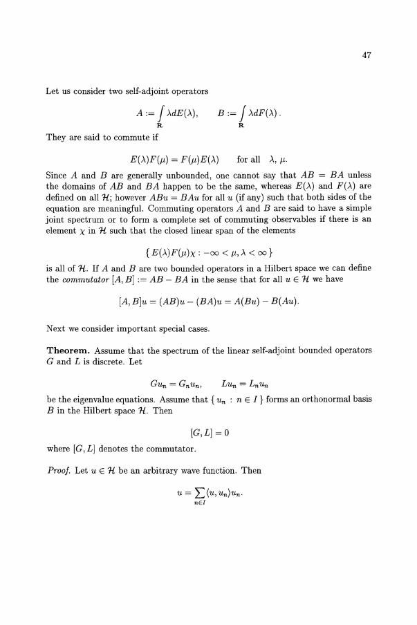
Let us consider two self-adjoint operators
A := f >.dE(>.), R
They are said to commute if
B := f >.dF(>.) . R
E(>.)F(p,) = F(p,)E(>') for all >., p,.
47
Since A and B are generally unbounded, one cannot say that AB = BA unless the domains of AB and BA happen to be the same, whereas E(>') and F(>') are defined on all 1£; however ABu = BAu for all u (if any) such that both sides of the equation are meaningful. Commuting operators A and B are said to have a simple joint spectrum or to form a complete set of commuting observables if there is an element X in 1£ such that the closed linear span of the elements
{E(>')F(p,)X : -00 < p" >. < 00 }
is all of 1£. If A and B are two bounded operators in a Hilbert space we can define the commutator [A, B] := AB - BA in the sense that for all u E 1£ we have
[A, B]u = (AB)u - (BA)u = A(Bu) - B(Au).
Next we consider important special cases.
Theorem. Assume that the spectrum of the linear self-adjoint bounded operators G and L is discrete. Let
be the eigenvalue equations. Assume that {un : n E I} forms an orthonormal basis B in the Hilbert space 1£. Then
[G,L]=O
where [G, L] denotes the commutator.
Proof. Let u E 1£ be an arbitrary wave function. Then
u = L (u, un}un. nEI
48 CHAPTER 3. LINEAR OPERATORS IN HILBERT SPACES
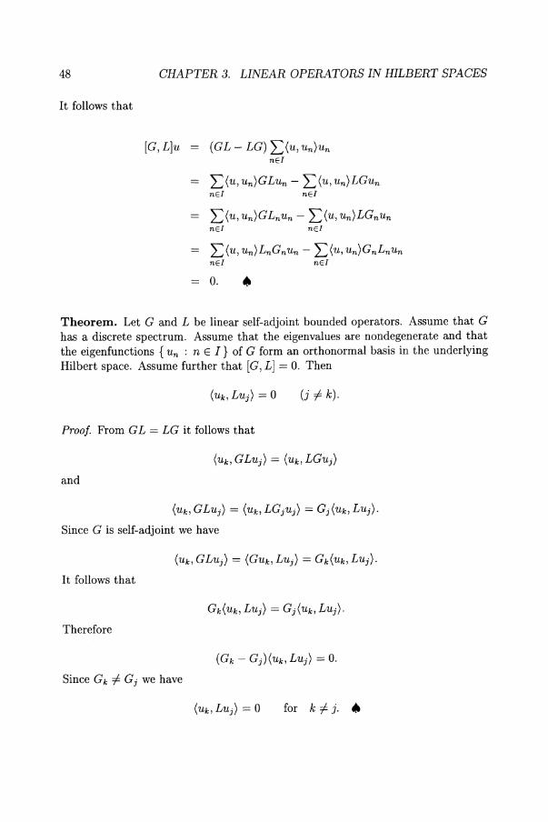
It follows that
[G,L]u (GL - LG) E(u, Un)Un nEI
nEI nEI
E(u,un)GLnun - E(u,un)LGnun nEI nEI
= E(u, un)LnGnun - E(u, un)GnLnun nEI nEI
o. •
Theorem. Let G and L be linear self-adjoint bounded operators. Assume that G has a discrete spectrum. Assume that the eigenvalues are non degenerate and that the eigenfunctions {un : n E I} of G form an orthonormal basis in the underlying Hilbert space. Assume further that [G, L] = o. Then
(j =f. k).
Proof. From G L = LG it follows that
and
(Uk, GLUj) = (Uk, LGjUj) = Gj(Uk, LUj).
Since G is self-adjoint we have
It follows that
Therefore
Since Gk =f. Gj we have
for k =f. j. •
49
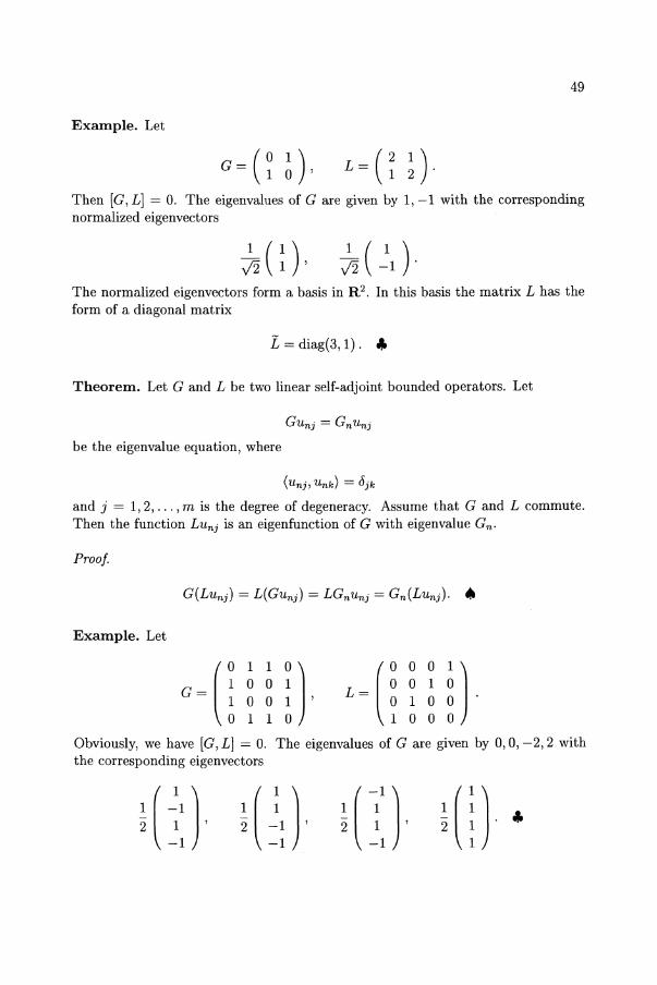
Example. Let
Then [G, L] = o. The eigenvalues of G are given by 1, -1 with the corresponding normalized eigenvectors
The normalized eigenvectors form a basis in R2. In this basis the matrix L has the form of a diagonal matrix
I = diag(3, 1). ..
Theorem. Let G and L be two linear self-adjoint bounded operators. Let
be the eigenvalue equation, where
(Unj, Unk) = c5jk
and j = 1,2, ... , m is the degree of degeneracy. Assume that G and L commute. Then the function LUnj is an eigenfunction of G with eigenvalue Gn ·
Proof.
Example. Let
(01 1 0) 100 1
G= 1 0 0 1 ' o 1 1 0
(0 0 0 1) o 0 1 0
L= 0 1 0 0 . 1 000
Obviously, we have [G, L] = o. The eigenvalues of G are given by 0,0, -2,2 with the corresponding eigenvectors
50 CHAPTER 3. LINEAR OPERATORS IN HILBERT SPACES
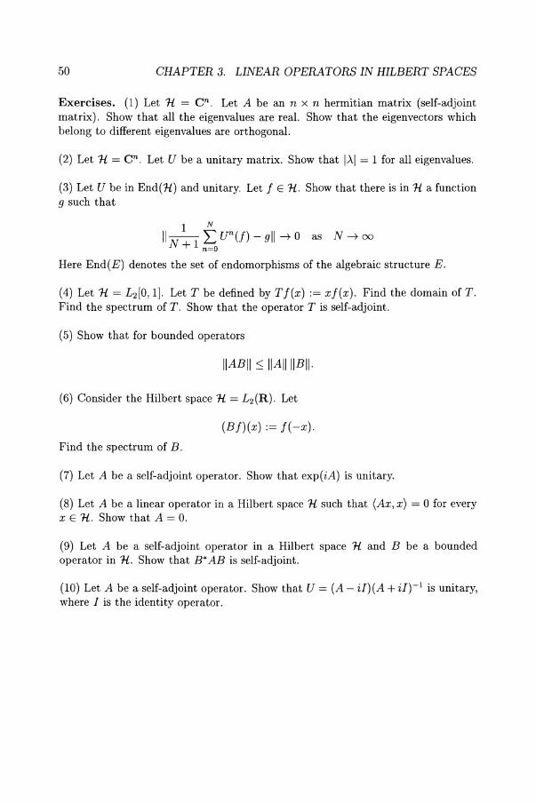
Exercises. (1) Let 1l = en. Let A be an n x n hermitian matrix (self-adjoint matrix). Show that all the eigenvalues are real. Show that the eigenvectors which belong to different eigenvalues are orthogonal.
(2) Let 1l = en. Let U be a unitary matrix. Show that IAI = 1 for all eigenvalues.
(3) Let U be in End(1l) and unitary. Let f E 1l. Show that there is in 1l a function 9 such that
1 N II-N L Un(f) - 911-+ 0 as N -+ 00
+ 1 n=O
Here End(E) denotes the set of endomorphisms of the algebraic structure E.
(4) Let 1l = L2[0, 1]. Let T be defined by Tf(x) := xf(x). Find the domain of T. Find the spectrum of T. Show that the operator T is self-adjoint.
(5) Show that for bounded operators
IIABII ~ IIAIIIIBII·
(6) Consider the Hilbert space 1l = L2(R). Let
(Bf)(x) := fe-x).
Find the spectrum of B.
(7) Let A be a self-adjoint operator. Show that exp(iA) is unitary.
(8) Let A be a linear operator in a Hilbert space 1l such that (Ax, x) = 0 for every x E 1l. Show that A = o.
(9) Let A be a self-adjoint operator in a Hilbert space 1l and B be a bounded operator in 1l. Show that B* AB is self-adjoint.
(10) Let A be a self-adjoint operator. Show that U = (A - iI)(A + iI)-l is unitary, where I is the identity operator.
Chapter 4
Generalized Functions
Besides Hilbert spaces generalized functions (Gelfand and Shilov [25], Vladimorov [67]) play an important role in quantum mechanics. In this chapter we give a short introduction to generalized functions.
Definition. Let S(R") be the set of all infinitely differentiable functions which decrease as Ixl -t 00, together with all their derivatives, faster than any power of Ixl-l . These functions are called test functions. It is obvious that S(R") C L2 (R") and S(Rn) is dense in L2(Rn).
Examples. e-x2 E S(R) and x4e-x2 E S(R). However, 1/(1 + X2) ¢ S(R), but 1/(1 + X2) E L2(R). ..
The convergence of test functions is defined as follows.
Definition. The sequence of functions (PI, ¢2, ¢3, ... , belonging to S(R") converges to the function ¢ E S(Rn), ¢k -t ¢ as k -t 00 in S(Rn), if for all a and f3
where we used the notation
x E R"
DO; alo;l -
8xf18x~2 ... ax~n
lal .- al +a2+' .. +an
xfi fi1 fi2 fin - Xl X 2 .• . X" .
51
W.-H. Steeb, Hilbert Spaces, Wavelets, Generalised Functions and Modern Quantum Mechanics© Kluwer Academic Publishers 1998
52 CHAPTER 4. GENERALIZED FUNCTIONS
Definition. A functional is a mapping from a linear space L into R (or C). Let T be the functional. Then (T, c/J) E R or C, where c/J E L.
A functional is called linear if (c/Jb c/J2 E L)
where Cl, C2 E C.
Example 1. Consider a Hilbert space 1£. Then the scalar product (.,.) defines a linear functional. "
Example 2. Consider the linear space of all n x n matrices. Then the trace of the matrices defines a linear functional, since tr(A + B) = trA + trB and tr(cA) = ctrA. The determinant of the n x n matrices defines a nonlinear functional, since det(A + B) 1= det A + det B in general. "
Generalized functions are special linear functionals. With the definitions given above we are ready to introduce the definition of a generalized function.
Definition. Each linear continuous functional over the space S(Rn) is called a generalized function (of slow growth).
The set of all generalized functions is denoted by: S'(Rn).
The convergence of generalized functions is defined as follows.
Definition. The sequence of generalized functions Tl , T2 , T3 , ... belonging to S'(Rn) converges to the generalized function T E S'(Rn) if for any c/J E S(Rn),
as k -t 00.
Let us now give three examples of generalized functions.
Example 1. If f is a locally integrable function of polynomial (slow) growth at infinity, that is for a certain m 2:: 0
/ If(x) I (1 + Ixl)-m dx < 00
Rn
then it defines a regular functional belonging to S'(Rn)
(f, c/J) : = J f(x)c/J(x) dx. Rn
As an application let
f(x) = { ~ x~o
x < o. The function f is called the step function. Then
00 (j, cjJ) = / f(x)cjJ(x) dx = / cjJ(x) dx. ..
R 0
53
Example 2. The delta function (also called the Dirac delta function) is defined by
(b(x), cjJ(x))
(b(x - xo), cjJ(x))
cjJ(O)
cjJ(xo).
The delta function b is a singular generalized function. ..
Example. The function l/x does not define a generalized function. However
p /00 cjJ(x) dx:= lim (/-< cjJ(x) dx + /00 cjJ(x) dX) x <-++0 X X
-00 00 €
defines a generalized function. Here P denotes the Cauchy principal value. For example, if c > 0, then
c d P / : =0.
-c
The differentiation of a generalized function T is defined as:
Definition. Let cjJ be a test function. Then the derivative of a generalized function T is defined as
where j = 1,2, ... , n and x = (Xl, X2, ... , xn ).
The motivation of this definition is as follows (for the case n = 1). Let f and 9 be two differentiable functions and f, 9 E L2(R). Integration by parts yields
/ df +00 / dg -gdx = fgl_ - f - dx. dx 00 dx R R
54 CHAPTER 4. GENERALIZED FUNCTIONS
The first term on the right hand side vanishes. It follows that
/ df / dg -gdx = - f -dx. dx dx
R R
Example. Let T be the generalized function generated by the step function. Then
( dT) (d¢) /00 d¢ dx' ¢ : = - T, dx = - dx dx = ¢(O) = (6(x), ¢(x)). o
In short hand notation we have
dT = J: ....
dx u. ..
For higher derivatives we have
Now we introduce the Fourier transform of a generalized function. First we have to give the Fourier transform of a test function.
Definition. Let ¢ E S(Rn). The Fourier transform in the ordinary sense (see chapter 2) is defined by
'lj;(k) := F[¢] : = / ¢(x)eik.x dx Rn
where
It follows that 'lj; E S(Rn). The Fourier transform operation is continuous from S(Rn) to S(Rn). The inverse transformation is given by
¢(x) = (2!)n / 'lj;(k)e-ik.x dk Rn
where
dk := dk1dk2 ... dkn .
The Fourier transform is a unitary transformation. A consequence of the definitions given above is
55
Definition. Let ¢ be a test function, i.e. ¢ E S(Rn) and T be a generalized function. Then the Fourier transform F(T) of the generalized function T is defined as
where
'I/>(k) == F[¢(x)] = J ¢(x)eik.x dx. Rn
The Fourier transform operation is continuous from S'(Rn) to S'(Rn).
Example. Let T be the generalized function generated by f(x) = 1. Then
Since
it follows that
Consequently,
(F(T), '1/» : = 27r(I, ¢) = 27r J ¢(x) dx. R
'I/>(k) = J ¢(x)eikx dx R
'1/>(0) = J ¢(x)dx. R
(F(T), '1/» = 27r'l/>(0) = 27r(J(k), 'I/>(k)).
In short hand notation we write
F[l] = 27rJ. ..
Example. Let T be the generalized function generated by exp(cx). Then
F[exp(cx)] = 27rJ(k - ic). ..
The tensor product (direct product) is defined as follows. Let f E S'(Rn) and 9 E S'(Rm). Then
(f(x) 0 g(y), ¢(x, y)) := (f(x) , (g(y), ¢(x, y))).
It can be proved that the right hand side is a linear continuous functional over S(Rn+m). The tensor product of generalized functions is commutative and associative in S'.
56 CHAPTER 4. GENERALIZED FUNCTIONS
Example. Let
H(x) := { ~ if Xj 2: 0 for all j = 1,2, ... ,n otherwise
be the Heaviside function defined on R n. Then
or considered as a functional
H(x) = H(Xl) 0 H(X2) 0 ... 0 H(xn) .
Then we find for the derivative in the sense of generalized functions
Next we summarize the "cooking recipe" for the delta function. These cooking recipes are used quite often in physics. If properly applied the results are correct.
with
{ (X) x=O b x = ( ) 0 otherwise
-,( {(X) x = Xo uX-x -0) - 0 otherwise
J b(x)dx = 1, R
J b(x - xo)dx = 1 R
J b(x)f(x)dx = f(O), J b(x - xo)f(x)dx = f(xo). R R
Analogously, in the discrete case we have
2:bjmaj = am JEI
where bjm denotes the Kronecker delta.
where a i- O.
J e-ikxb(x)dx = 1, R
1 b(ax) = ~b(x)
J eikxdk = 27rb(x) R
b(x) = b(-x)
where
1 8(a2 - x2 ) = 2a {8(x + a) + 8(x - an, a> 0
~O 8(x - Xi)
d~~) = 8(x), dO(x - xo) = 8(x - xo) dx
O(x - xo) = { ~ if X ~ Xo
otherwise
r 1 E 8(x) Im--- = <-40 7r x2 + E2
r 1 sinnx 8(x) Im---n-4oo 7r X
r 1 -x2 /4t 1m --e H+O 2.,fii 8(x)
r 1 Im--<-40 X + iE
= p(~) -i7r8(x)
57
where P denotes the Cauchy principal value. The convergence is obviously convergence in the sense of generalized functions. The Cauchy principal value is defined as
P -l f(x)dx := <!1~0 Cl f(x)dx + 1 f(x)dx ) .
In practical applications the following identity is useful. Let f be a smooth function with simple zeros. Then
where the sum runs over all zeros and f'(xn ) denotes the derivative of f taken at x n ·
Example. Let f(x) = sin(x). Then
8(sin{x)) == L 8(x - 7rn) . • nEZ
58 CHAPTER 4. GENERALIZED FUNCTIONS
In scattering theory we need the so-called fundamental solution of the Helmholtz equation in three dimensions.
Definition. Let L(D) be a linear differential operator with constant coefficients
where
m
L(D) = ~ anD'" Inl=O
D:= (",0 ,,,,0 , ... , ",0 ) . UXI UX2 UXn
The generalized function £ E S'(Rn) which satisfies the equation (in the sense of generalized functions)
L(D)£ = J
is said to be the fundamental solution of the differential operator L(D), where J denotes the delta function.
The fundamental solution £ of the operator L(D) is not unique. Let £0 be an arbitary solution of the homogeneous equation
L(D)£o = O.
The generalized function £ +£0 is also a fundamental solution of the operator L(D).
In order that the generalized function £ E S'(Rn) should be the fundamental solution of the operator L(D), it is necessary and sufficient that its Fourier transform F(£) satisfies the equation
L( -i~)F(£) = 1
where
m
L(~) = ~ aae. Inl=O
Example. Consider the differential equation in the sense of generalized functions
where
59
The Fourier transform in the sense of generalized functions leads to
(-leI2 + k2)F(cn ) = l.
The fundamental solution for n = 3 is given by
where Ixl = vx~ + x~ + x~. "
Eigenvalue problems can also be considered in the space of generalized functions.
Definition. Let A be a linear operator in a linear topological space L. A linear functional F on ¢, such that
(AF, ¢) = A(F, ¢)
for every element ¢ E L, is called a generalized eigenvector of the operator A, corresponding to the eigenvalue A, where
(AF, ¢) = (AF, ¢) = F(A*¢).
In the following the topologoical space under consideration is L = S(Rn). Let us consider two examples.
Example 1. Consider the operator -id/dx defined on S(R) C L2(R). The eigenvalue equation is takes the form
_id~~) = Af(x).
The solution is given by
However
ei>..x f/. S(R),
Consider the differential operator -id/dx in the space S'(R). Then obviously we find that
f(x) = ei>..x
is a generalized eigenvector and A E R, i.e. the spectrum is the real axis. The generalized function given by the function ei>..x is
(ei>"x,¢(x)) = ! e-i>"x¢(x)dx. " R
60 CHAPTER 4. GENERALIZED FUNCTIONS
Remark. If we consider complex valued test functions and generalized functions, then we have
c(T, </» = (cT, </» = (T, c</»
and
(1, </» = J J</>dx Rn
where f is a regular functional and c E C.
Example 2. Consider the eigenvalue equation
xf(x) = )..j(x).
There is no solution in the Hilbert space L2(R). However there is a solution in the sense of generalized functions
(x8(x - >'), </>(x)) = (8(x - >'), x</>(x)) = >'(8(x - >'), </>(x))
where>. E R. The "eigenfunction" is the delta function. Here we used the fact that
(xT,</» = (T,x</» . ..
Exercises. (1) Let
Show that
{ t; for Ixl::; a fa(x) = 0 for Ixl > a.
J fa (x)dx = l. R
61
Find lima-+o fa in the sense of generalized functions. Calculate the derivative of fa in the sense of generalized functions. What happens if a -+ 0 ?
(2) Let E > 0 and
f,(x) = { C, exp ( - ,2~~xI2) Ixl < E o Ixl 2: E
where Ixl = JXI + x~ + ... + x~. We choose C, so that
J f,(x)dx = l. Rn
Show that
limf,(x) = b(x) ,-+0
in the sense of generalized functions.
(3) Find the derivative of I cos(x)1 in the sense of generalized functions.
(4) Show that
1 f eikx = f b(x - 2k1r). 27r k==-oo k==-oo
(5) Show that in the sense of generalized functions
f sin(nx) == ! cot (~) n==l 2 2
(6) Show that the Fourier transform of cosh(at) in the sense of generalized functions is given by
7r(b(w - ia) + b(w + ia)) .
62 CHAPTER 4. GENERALIZED FUNCTIONS
(7) Find a generalized function F(t) := H(t)f(t) where H is the Heaviside function and f is a smooth function such that F satisfies the differential equation in the sense of generalized functions
d2F dF I
a dt2 + bdi + cF = mJ + nJ .
Here a, b, c, m and n are nonzero constants.
(8) Show that
£(x t) - O(t) ex (_ Ixl2 )
, - (2aJ:;rt)n p 4a2t
is the fundamental solution of the heat conduction operator, i.e.
o£ at - a2 !:J.£ = J(x, t)
where 0 is the step function and
(9) Let
Show that
!:J.ln Ixl = 21fJ(x)
in the sense of generalized functions.
(10) Let H be the Heaviside function. Let
H(t) (_X2) E(x, t):= c; exp - . 2V1ft 4t
Calculate
ot ox2 '
Chapter 5
Classical Mechanics and Hamilton Systems
In classical mechanics (Arnold [2]) we consider the phase space
R 6N = {(p, q)}
where
Here N is the number of particles, p are the momenta and q are the coordinates.
Many dynamical systems can be described in nonrelativistic mechanics by a Hamilton function
H(p, q) = Hkin(P) + V(q).
The first term on the right hand side is the kinetic part and the second term is the potential. The kinetic part is given by
where mk is the mass of the k-th particle.
The Hamilton equations of motion are given by
63
W.-H. Steeb, Hilbert Spaces, Wavelets, Generalised Functions and Modern Quantum Mechanics© Kluwer Academic Publishers 1998
64 CHAPTER 5. CLASSICAL MECHANICS AND HAMILTON SYSTEMS
dqkj 8H dt = 8Pkj·
It follows that
dPkj 8V dt - 8qkj'
or
cf2qkj 1 8V dt2 - mk 8qkj .
The initial value problem is as follows. Given
Find
with t > o.
If the Hamilton function H does not depend explicitly on time, then the phase trajectories of the Hamilton equations of motion lying on the surface
M 6N- 1 : H(p,q) = E
are extremals of the integral J pdq in the class of curves lying on M 6N -1 and connecting the subspaces q = qo and q = q1. The energy E is given by the initial values.
Simple examples of Hamilton systems are
(i) harmonic oscillator in one dimension
(ii) freely falling body
1 2 2 2) H(p, q) = 2m (P1 + P2 + Pa + mgqa
(iii) pendulum 1 p2
H(p(},()) = --% - mgrcos() 2mr
For all these cases we can find the solutions explicitly.
65
For the pendulum the equations of motion are given by
dpo oH . () dt = - o() = -mgrsm
d() oH 1 = -=--Po·
dt OPIJ mr2
In order to solve the Hamilton equations of motion we first have to find out whether first integrals exist for the dynamical system.
Definition. A smooth function f is called a first integral of the Hamilton equations of motion if
d d/(P(t), q(t)) = O.
Applying the chain rule it follows that
ft (Of dPkj + of dqkj ) = O. k=l j=l 0Pkj dt Oqkj dt
Inserting the Hamilton equations of motion we arrive at
Obviously, the Hamilton function H is a first integral. In general, there are no other first integrals. In most cases the solution of the Hamilton equations of motion can only be found numerically.
Remark. Let f(p, q) and g(p, q) be two smooth functions. The Poisson bracket is defined as
{f,g}:=ft(Of og _ of (9). k=l j=l Oqkj OPkj OPkj Oqkj
Thus the condition that f is a first integral can be written as {j, H} = O.
Let us give two examples where we find another first integral (besides the Hamilton function).
Example 1. For a system of N particles with central two-body interaction described by the Hamilton function
66 CHAPTER 5. CLASSICAL MECHANICS AND HAMILTON SYSTEMS
where
Iqk - qll := V(qkl - qn)2 + (qk2 - q12)2 + (qk3 - qI3)2.
The first integrals are given by
pkin J
H
N
LPkj k=l
N
L(qkiPkj - qkjPki) k=l
where j = 1,2,3 and
with
Momentum
Angular momentum
Hamilton function
centre of gravity
Example 2. Consider the Hamilton function
with two degrees of freedom, where a E [0,1]. For a = 0 we find the first integral
For all other values of a we do not find a first integral (besides the Hamilton func
tion). "
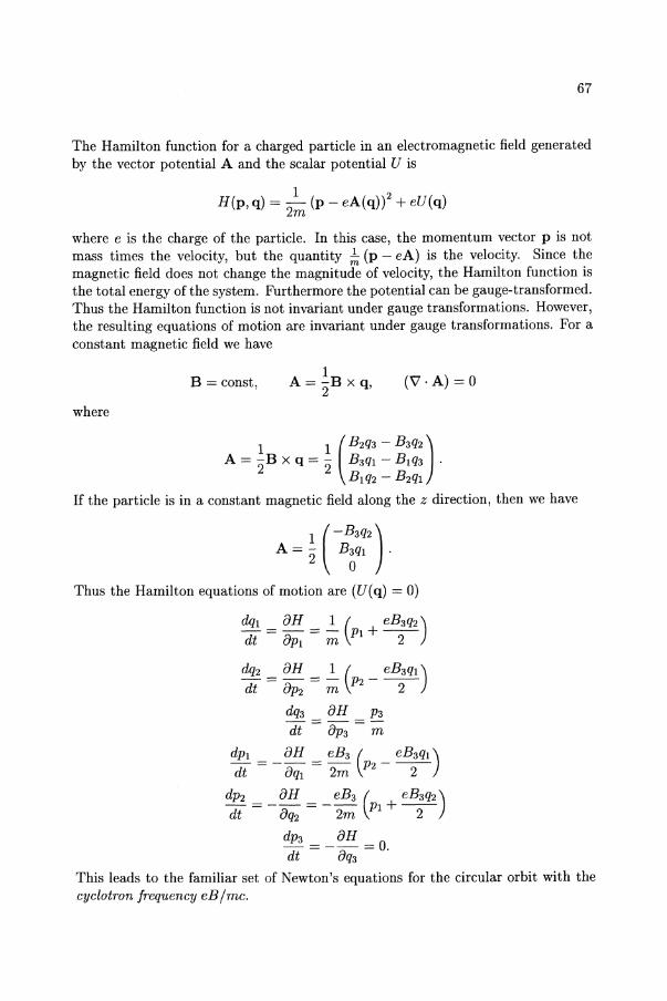
67
The Hamilton function for a charged particle in an electromagnetic field generated by the vector potential A and the scalar potential U is
1 2 H(p, q) = 2m (p - eA(q)) + eU(q)
where e is the charge of the particle. In this case, the momentum vector p is not mass times the velocity, but the quantity ~ (p - eA) is the velocity. Since the magnetic field does not change the magnitude of velocity, the Hamilton function is the total energy of the system. Furthermore the potential can be gauge-transformed. Thus the Hamilton function is not invariant under gauge transformations. However, the resulting equations of motion are invariant under gauge transformations. For a constant magnetic field we have
where
B = const, 1
A="2B x q, (\7. A) = 0
1 1 (B2q3 - B3q2) A="2Bxq ="2 B3ql-B1q3 .
B 1q2 - B2ql
If the particle is in a constant magnetic field along the z direction, then we have
h~C~~;') Thus the Hamilton equations of motion are (U(q) = 0)
dql = 8H = ~ (PI + eB3q2) dt 8PI m 2
dq2 = 8H = ~ (P2 _ eB3ql) dt 8P2 m 2
dq3 8H P3 = dt 8P3 m
dPI = _ 8H = eB3 (P2 _ eB3ql) dt 8ql 2m 2
dP2 = _ 8H = _ eB3 (PI + eB3q2) dt 8q2 2m 2
dpa = _ 8H = o. dt 8q3
This leads to the familiar set of Newton's equations for the circular orbit with the cyclotron frequency eB I me.
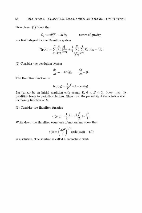
68 CHAPTER 5. CLASSICAL MECHANICS AND HAMILTON SYSTEMS
Exercises. (1) Show that
OJ := tPjkin - MRj
is a first integral for the Hamilton system
(2) Consider the pendulum system
dp . ( ) dt=-sm q ,
The Hamilton function is
centre of gravity
dq -=p. dt
1 H(p, q) = 2l + 1 - cos(q) .
Let (qo,Po) be an initial condition with energy E, 0 < E < 2. Show that this condition leads to periodic solutions. Show that the period To of the solution is an increasing function of E.
(3) Consider the Hamilton function
1 2 2q2 q4 H(p, q) = 2P - w 2 + c"4'
Write down the Hamilton equations of motion and show that
(2 2) 1/2
q(t) = ~ sech (±w(t - to))
is a solution. The solution is called a homo clinic orbit.
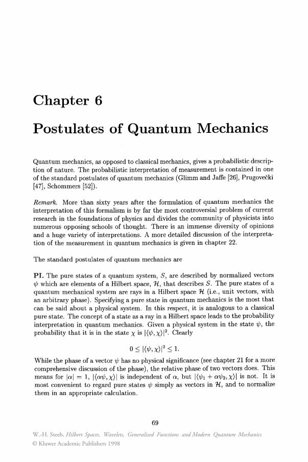
Chapter 6
Postulates of Quantum Mechanics
Quantum mechanics, as opposed to classical mechanics, gives a probabilistic description of nature. The probabilistic interpretation of measurement is contained in one of the standard postulates of quantum mechanics (Glimm and Jaffe [26], Prugovecki [47], Schommers [52]).
Remark. More than sixty years after the formulation of quantum mechanics the interpretation of this formalism is by far the most controversial problem of current research in the foundations of physics and divides the community of physicists into numerous opposing schools of thought. There is an immense diversity of opinions and a huge variety of interpretations. A more detailed discussion of the interpretation of the measurement in quantum mechanics is given in chapter 22.
The standard postulates of quantum mechanics are
PI. The pure states of a quantum system, S, are described by normalized vectors 'IjJ which are elements of a Hilbert space, 1£, that describes S. The pure states of a quantum mechanical system are rays in a Hilbert space 1£ (i.e., unit vectors, with an arbitrary phase). Specifying a pure state in quantum mechanics is the most that can be said about a physical system. In this respect, it is analogous to a classical pure state. The concept of a state as a ray in a Hilbert space leads to the probability interpretation in quantum mechanics. Given a physical system in the state 'IjJ, the probability that it is in the state X is 1('IjJ, xW. Clearly
o ~ 1('IjJ,xW ~ l. While the phase of a vector 'IjJ has no physical significance (see chapter 21 for a more comprehensive discussion of the phase), the relative phase of two vectors does. This means for lal = 1, l(a1jJ,x)1 is independent of a, but 1('ljJl + a1jJ2,x)1 is not. It is most convenient to regard pure states 1jJ simply as vectors in 1£, and to normalize them in an appropriate calculation.
69
W.-H. Steeb, Hilbert Spaces, Wavelets, Generalised Functions and Modern Quantum Mechanics© Kluwer Academic Publishers 1998
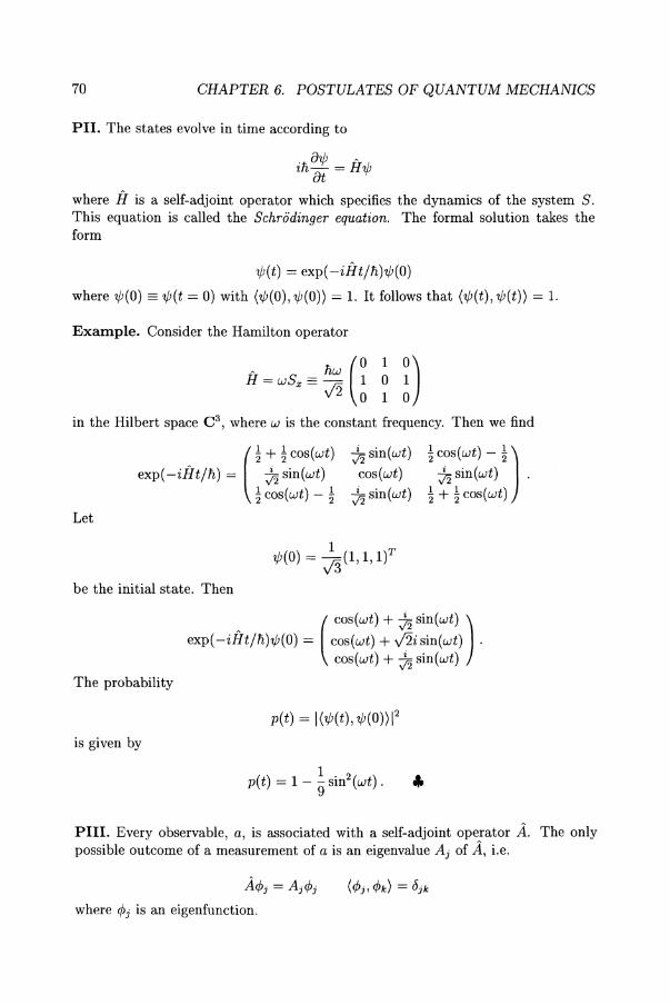
70 CHAPTER 6. POSTULATES OF QUANTUM MECHANICS
PII. The states evolve in time according to
it/N = H1/; at
where H is a self-adjoint operator which specifies the dynamics of the system S. This equation is called the Schrodinger equation. The formal solution takes the form
1/;(t) = exp( -iHt/h)1/;(O)
where 1/;(0) == 1/;(t = 0) with (1/;(0),1/;(0)) = 1. It follows that (1/;(t) , 1/;(t)) = 1.
Example. Consider the Hamilton operator
H~wS.= ~ G ~ n in the Hilbert space C3 , where w is the constant frequency. Then we find
( ~ + ~ cos(wt) 0 sin(wt)
exp( -iHt/h) = 0 sin(wt) cos(wt) ~ cos(wt) - ~ 0 sin(wt)
~ c~s(~t) - ~) v'2 sm(wt) .
~ + ~ cos(wt)
Let
1 )T 1/;(0) = J3(1, 1, 1
be the initial state. Then
( cos(wt) + 0 sin(wt) )
exp( -iHt/h)1/;(O) = cos(wt) + V2i sin(wt) . cos(wt) + ~ sin(wt)
The probability
p(t) = 1(1/;(t),1/;(0))12
is given by
p(t} = 1 - ~ sin2 (wt) . .,.
PIlI. Every observable, a, is associated with a self-adjoint operator A. The only possible outcome of a measurement of a is an eigenvalue Aj of A, i.e.
A<pj = Aj<pj
where <Pj is an eigenfunction.
71
PIV. If the state of the system is described by the normalized vector 'lj;, then a measurement of a will yield the eigenvalue Aj with probability
Pj = 1(<pj,'lj;W·
Notice that (<pj, 'lj;) can be complex. It is obvious that 0 ::; Pj ::; 1.
In order for successive measurements of a to yield the same value Aj it is necessary to have the projection postulate:
PV. Immediately after a measurement which yields the value Aj the state of the system is described by <Pi'
The type of time evolution implied by PV is incompatible with the unitary time evolution implied by PlI. PIV can be replaced by the weaker postulate:
PIV'. If a quantum system is described by the state <Pj then a measurement of a will yield the value Aj .
Clearly PIV' is a special case of PIV but it is not a statement about probabilities. The replacement of PIV by PlY' eliminates the immediate need for PV since the state is <Pi before and after the measurement.
PVI. Quantum mechanical observables are self-adjoint operators on 1l. The expected (average) value of the observable b with the corresponding self-adjoint operator B in the normalized state 'lj; is
E",(B} := ('lj;, B'lj;).
Examples of observables are the Hamiltonian (energy) observable, the momentum observable, and the position observable.
The statistical mixtures in quantum mechanics lead to quantum statistical mechanics. The usual statistical mixture is described by a positive trace class operator p, yielding the expectation
p(B) = tr(pB} trp
where tr denotes the trace. If p has rank 1, then p(B) is a pure state with p/trp the projection onto 'lj;. Otherwise, p(B) is a convex linear combination of pure states,
p(B} = L O!j(<Pj, B<pj) j
where the <Pj are the (orthonormal) eigenvectors of p and Ej O!j = 1.
72 CHAPTER 6. POSTULATES OF QUANTUM MECHANICS
PVII. The Hamilton operator H is the infinitesimal generator of the unitary group
U(t) := exp( -itH In) of time translations. The unit of action n (hI27r) has the same dimension as pq.
The momentum operator p is the infinitesimal generator of the unitary space translation group
exp(iq· PIn) where
N 3
q. p:= L LqkjPkj. k=lj=l
We recall that
exp(a· V)u(q) = u(q + a)
where u is a smooth function and
N 3 8 a·V:= LLakj-
k=lj=l 8qkj
The angular momentum operator j is the infinitesimal generator for the unitary space rotation group
exp( -if} . j).
Remark. This leads to the quantization. Consider the energy conservation equation
N 3 2
E = LL Pkj + V(q). k=lj=1 2mk
We make the formal substitution
We arrive at the formal operator relation
.t. 8 Pkj -+ -Zn--.
8qkj
8 N 3 n2 82
in-=-LL--2 +V(q). 8t k=l j=l 2mk 8qkj
Applying this operator relation to a wave function '¢'(q, t) we obtain the Schr6dinger equation.
73
The time translation group U(t) determines the dynamics. There are two standard descriptions: the Schrodinger picture and the Heisenberg picture. In the Schri:idinger picture, the states 'ljJ E 1l evolve in time according to the Schri:idinger equation, while the observables do not evolve. The vectors satisfy the Schri:idinger equation. The time-dependent normalized state 'ljJ(t) yields the expectation
E.p(t)(B) = ('ljJ(t) , B'ljJ(t)).
The second description of dynamics is the Heisenberg picture, in which the states remain fixed, and the observables evolve in time according to the automorphism group
B ---+ B(t) = eitH/r. Be-itH/r. = U(t)* BU(t).
Obviously we assume that the Hamilton operator does not depend explicitly on t. Thus the observables B satisfy the dynamical equation (Heisenberg equation of motion)
-in d~;t) = [iI, B(t)]
with the formal solution
00 (it/n)n, , , . ' . ' B(t) = L -,-[H, [H, . .. , [H, BJ, ... J] = exp(zHt/n)B exp( -zHt/n) .
n=O n.
The relation between the Heisenberg and Schri:idinger pictures is given by
('ljJ(t) , B'ljJ(t)) = ('ljJ, B(t)'ljJ)
where 'ljJ = 'ljJ(t = 0).
Postulate PVII ensures that the results of an experiment, i.e., inner products ('ljJ, X), are independent of the time at which the experiment is performed. This means
1('ljJ,x)1 = 1('ljJ(t),x(t))I·
Theorem. Every symmetry of 1l can be implemented either by a unitary transformation U on 1l,
'ljJ' = U'ljJ
or by an antiunitary operator A on 1l
'ljJ'=A'ljJ.
74 CHAPTER 6. POSTULATES OF QUANTUM MECHANICS
The interpretation of this result is that every symmetry of 1i can be regarded as a coordinate transformation. In particular, the group of time translations is implemented by a unitary group of operators U(t). Only certain discrete symmetries (e.g., time inversion in nonrelativistic quantum mechanics) are implemented by antiunitary transformations.
Example. In nonrelativistic quantum mechanics one usual representation for a system of N particles moving in a potential V is
1i = L 2(R3N ).
This choice is called the Schrodinger representation (as distinct from the Schrodinger picture). The function 1/'(q) E 1i has the interpretation of giving the probability distribution
p(q) = 11/'(q)12
for the position of the particles in R 3N. Using postulate PVII, we find
A 'fc; 0 Pk' ---+ Pk' = -Zn--
J J Oqkj
and a nonrelativistic Hamilton function of the form
N 3 2
H=LL Pkj +V(q) k=lj=1 2mk
becomes the elliptic differential operator
A N 3 fi2 02 A
H=-LL--2 +V(q). k=l j=l 2mk Oqkj
In other words the Hamilton operator fI follows from the Hamilton function H via the quantization
. 0 Pkj ---+ -zfi--
Oqkj
qkj ---+ iikj.
The operator iikj is defined by iikjf(q) .- qkjf(q). We find for the (canonical) commutation relations
[iikj, iiklj'] 0
[Pkj,Pk1jl] 0
[Pkj, iiklj'] -iMkk'ojj,J
75
(see chapter 11 for more details). They are preserved by the Heisenberg equation of motion. .,.
Thus far the spin of the particle is not taken into account. We have spin 0 for 7r
mesons, spin ~ for electrons, muons, protons, or neutrons, spin 1 for photons, and higher spins for other particles or nuclei. To consider spin-dependent forces (for example the coupling of the spin magnetic moment to a magnetic field) we have to extend the Hilbert space L 2 (R3N ) to the N-fold tensor product
1£ = ®L2(R3 , S).
Here L 2 (R3 , S) denotes functions defined on R 3N with values in the finite dimensional spin space S. For spin zero particles we have S = C, and we are reduced to L2 (R3N). For nonzero spin s, we have S = C 28+1. We write 1jJ(q) as a vector with components 1jJ(q, (). A space rotation (generated by the angular momentum observable J) will rotate both q and (, the latter by a linear transformation of the ( coordinates according to an N-fold tensor product of a representation of the spin group SU(2, R). The group SU(2, R) consists of all 2 x 2 matrices with
UU· = I
and
detU = 1
Particles of a given type are indistinguishable. To obtain indistinguishable particles, we restrict ourselves to a subset of ®L2 (R 3 , S) invariant under an irreducible representation of the symmetric group (permutation group) of the N particle coordinates (Qk, (k), k = 1,2, ... , N. The standard choices are the totally symmetric representation for integer spin particles and the totally antisymmetric representation for half-integer spin particles.
The choice of antisymmetry for atomic and molecular problems with spin ~ is known as the Pauli exclusion principle. One can prove that integer spin particles cannot be antisymmetrized and half-integer spin particles cannot be symmetrized. Particles with integer spin are called bosons. Those with half-integer spin are called fermions.
Postulate VIII. A quantum mechanical state is symmetric under the permutation of identical bosons, and antisymmetric under the permutation of identical fermions.
76 CHAPTER 6. POSTULATES OF QUANTUM MECHANICS
Exercises. (1) Consider the spin-l matrices
1i (0 1 0) Sx := . tri 1 0 1 , v 2 0 1 0
and the Hamilton operator
iI:= wSx •
Use the Heisenberg equation of motion to find the time-evolution of Sz. Let
1 )T 1P(0) = y'3(1, 1, 1 .
Find
('IjJ(O), Sz(t)1P(O)) .
(2) Let a E R. Show that
exp (a d~) x = x + a, exp (a :x) x2 = (x + a)2.
(3) Let a E R. Find
Chapter 7
Interaction Picture
Any change with time in the state of a quantum mechanical system can be described by keeping the axes fixed and allowing the state vector to rotate, or by keeping the state vector fixed and allowing the axes to rotate. The two possibilities described above are called Schrodinger and Heisenberg picture, respectively. Let iI be the Hamilton operator of the system. We assume that the Hamilton operator is selfadjoint.
In the Schrodinger picture we describe the time-evolution of the wave function 'ljJ. This means
In the Heisenberg picture we describe the time-evolution of the operator A, where [ , ] denotes the commutator. This means
We find that
where A == A(t = 0).
!1i~ = [A, iI](t),
A(O) ---t A(t)
('ljJ(t) , A'ljJ(t» = ('ljJ(0) , A(t)'ljJ(O))
77
W.-H. Steeb, Hilbert Spaces, Wavelets, Generalised Functions and Modern Quantum Mechanics© Kluwer Academic Publishers 1998
78 CHAPTER 7. INTERACTION PICTURE
Next we consider the interaction picture. We assume that the Hamilton operator is time independent and can be expressed as the sum of two terms
fI = fIo + V. We assume that the eigenvalues and eigenfunctions of fIo are known. We define the interaction state vector as
which is a unitary transformation carried out at the time t. The index S indicates the Schrodinger picture and the index I indicates the interaction picture. The equation of motion of this state vector is found by
Thus we obtain the following set of equations in the interaction picture
where we define
VI(t) := eiHot/nVe-iflot/n.
In general, fIo does not commute with V, so that the proper order of these operators is important. An arbitrary matrix element of an operator A in the Schrodinger picture may be written as
which suggests the following definition of an operator in the interaction picture
AI (t) == eiHot/n Ase-iHot/h,.
These equations show that the operator AI(t) and the state vectors I~h(t)) both depend on time in the interaction picture. Differentiating AI with respect to time yields
in :t AI(t) = eiliot/n(AsHo - HoAs)e-iHot/n = [AI(t), Ho].
Here the time independence of the Schrodinger operator has been used along with the observation that any function of an operator commutes with the operator itself.
We now solve the equations of motion in the interaction picture. Define a unitary operator U(t, to) that determines the state vector at time t in terms of the state vector at the time to
79
where U must satisfy the relation
U(to, to) = I. For finite times U(t, to) can be constructed explicitly by using the Schrodinger picture
l'ifr(t)) = eiHot/IiI'ifs(t)) = eiHot/lie-iH(t-to)/lie-iHoto/IiI'ifr(to))
where we used l'ifs(t)) = exp( -ifI(t - to)/n)I'ifs(to)). Consequently
U(t, to) = eiHot/lie-iH(t-to)/lie-iHoto/1i (finite times).
Since N and No do not commute with each other, the order of the operators must be maintained. We find that U has the properties
ut(t, to)U(t,to) = U(t,to)ut(t, to) = I
which implies that U is unitary. We write ut instead of U* in this chapter. Furthermore
which shows that U has the group property, and
U(t, to)U(to,t) = I which implies that
U(to, t) = ut(t, to).
We construct an integral equation for U, which can then be solved by iteration. It is clear that U satisfies the operator differential equation
a A
in at U(t, to) = V(t)U(t, to).
Integrating this equation from to to t gives
. t
U(t, to) - U(to, to) = -~ f dt'V(t')U(t', to). to
This result, combined with the boundary condition U(to, to) = I yields an integral equation
. t
U(t, to) = I - ~ f dt'V(t')U(t', to). to
80 CHAPTER 7. INTERACTION PICTURE
We solve this equation by iteration, always maintaining the proper ordering of the operators. The solution thus takes the form
. t . 2 t t!
U(t, to) = I + (~Z) J dt'V(t') + (~Z) J dt' J dt"V(t')V(t") + .... to to to
We consider the third term in this expansion. It may be rewritten as
t t! t t' 1 t t J dt' J dt"V(t')V(t") = ~ J dt' J dt"V(t')V(t") + 2 J dt" J dt'V(t')V(t") to to to to to til
since the last term on the right is just obtained by reversing the order of the integrations. We now change dummy variable in this second term, interchanging the labels t' and t". Hence
t t t t
~ J dt" J dt'V(t')V(t") = ~ J dt' J dt"V(t")V(t'). to til to t'
The two terms given above may now be combined to give
t t' t t J dt' J dt"V(t')V(t") = ~ J dt' J dt"[V(t')V(t")O(t' - t") + V(t")V(t')O(t" - t')] ~ ~ ~ ~
where 0 is the step function. Notice that the operators V(t) do not necessarily commute at different times. The operator containing the latest time stands farthest to the left. We call this a time-ordered product of operators, denoted by the symbol T. Thus we can write
t t' t t J dt' J dt"V(t')V(t") == ~ J dt' J dt"T[V(t')V(t")]. ~ ~ ~ ~
This result is readily generalized. The resulting expansion for U becomes
where the n = 0 term is just the unit operator I. The proof of this equation is as follows. Consider the nth term in this series. There are n! possible time orderings of the labels tl ... tn. Pick a particular one, say it > t2 > t3' .. > tn. Any other time ordering gives the same contribution to U. This result is seen by relabeling the dummy integration variables ti to agree with the previous ordering, and then using the symmetry of the T product under interchange of its arguments
81
This equation follows from the definition of the T product, which puts the operator at the latest time farthest to the left, the operator at the next latest time next, and so on.
Remark. The operator S = U(oo, -00) is called the S-matrix. Thus the operator S acting on the initial wave function of the system given as t -+ -00 gives the function of the system as t -+ 00.
Let us now describe that such an expansion leads in general to secular terms. Let 1£ be a Hilbert space, L the set of linear operators over 1£, Lh the subset of selfadjoint operators, and Ho, 11 E Lh. We want to find an approximate solution of the equation (we put Planck's constant equal to one)
.aU(t, f) A A
2 at = (Ho + fV)U(t, f).
The substitution
U(t, f) = exp( -iHot)U(t, f)
yields
where
V(t) := exp(itHo)V exp( -itHo).
This equation together with the initial condition U(O, f) = I is equivalent to the integral equation
t
U(t, f) = I - if J dsV(s)U(s, f). o
A formal solution of this equation is
00 t tl tk_l
U(t, f) = ~) -if)k J dt1 J dt2 . .. J dtk V(t1) •.. V(tk). k=O 0 0 0
In particular, the first approximation is
t
u(l)(t, f) = I - if J dsV(s). o
However this kind of pertubation expansion leads to secular terms, i.e. terms of the kind (ft)P, pEN. These terms obviously do not correspond to the general periodic behaviour of the exact solution.
82 CHAPTER 7. INTERACTION PICTURE
Example. Consider the weakly perturbed harmonic oscillator. Let
A 1 4 V(q) = 4q
where [p, q] = -i1 where [, ] stands for the commutator with Ii = 1. The linear transformation
A z+Z q= ffw'
with the inverse
leads to
and
Therefore
A 1 Ho = (N + 2)w,
[z,z] =1
A_I _ 4 V(z,z) = 16w2(z+z) .
V(z, z) = ~2 [3(1 + 2N + 2N2) + 2(31 + 2N)Z2 + z22(31 + 2N) + Z4 + z4] 16w
where N := zz. We denote the Hermitian conjugate of the operator z by z instead of the more usual z* or zt. We have N z = zN. It follows that
- 1 V(t) = -2 [3(1 + 2N + 2N2) + 2(31 + 2N)Z2 exp( -2iwt) 16w
+Z2 exp(2iwt)2(31 + 2N) + Z4 exp( -4iwt) + z4 exp(4iwt)].
Inserting this expression into
t
U(l)(t,f.) = 1 - if. J dsV(s) o
one obtains the secular term 3f.(1 +2N +2N2)t. Such secular terms may be voided by using the so-called avemging method. This method (Kummer [34]) can be described as follows. Let
:F = {flf = !;/(n)f.n; f(n) E L} be the set of formal power series with coefficients f(n) in C. Clearly U(t, f.) E :F. We represent U(t, f.) as a product
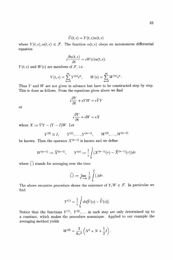
83
U(t, E) = Y(t, E)a(t, E)
where Y(t, E), a(t, E) E :F. The function a(t, E) obeys an autonomous differential equation
.aa(t, f) ()() t at = fW fat, f .
Y(t, E) and W(f) are members of F, i.e.
00
Y(t, f) = L y(n)fn ,
n=O n=O
Thus Y and Ware not given in advance but have to be constructed step by step. This is done as follows. From the equations given above we find
or
.ay t7)t + EW = EX
where X:= vy - (Y - I)W. Let
y(O) == I, y(l) y(n-l) , ... , , W(O) , ... , w(n-2)
be known. Then the operator x(n-l) is known and we define
W (n-l) .= x(n-l) . , t
y(n) := ~ / (x(n-l)(T) _ x(n-l) (T))dT
o
where (.) stands for averaging over the time
T
~ 1/ (.) := lim -T (.)dT. T-4OO
o The above recursive procedure shows the existence of Y, W E F. In particular we find
t
y(l) = ~ / ds[V(s) - V(s)]. o
Notice that the functions y(l), y(2), ... in each step are only determined up to a constant, which makes the procedure nonunique. Applied to our example the averaging method yields
84 CHAPTER 7. INTERACTION PICTURE
Exercises. (1) Let A, B be n x n matrices. Assume that
[A,B] = cI
where I is the n x n unit matrix and c is a constant. Show that
exp(A + B) == exp(A) exp(B) exp (-~CI) .
(2) Let Z be a linear operator depending smoothly on A. Show that
d /1 dZ(A) dA exp(Z) == dxexp(xZ(A))~exp(-xZ)exp(Z).
o
(3) Calculate y(I).
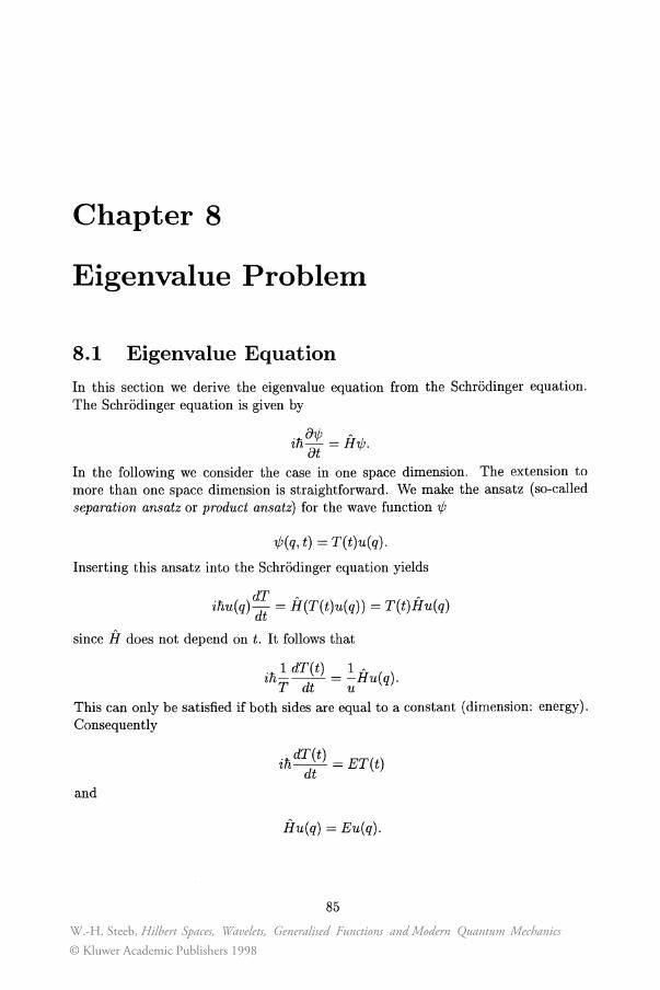
Chapter 8
Eigenvalue Problem
8.1 Eigenvalue Equation
In this section we derive the eigenvalue equation from the Schr6dinger equation. The Schr6dinger equation is given by
in ~~ = H1/1.
In the following we consider the case in one space dimension. The extension to more than one space dimension is straightforward. We make the ansatz (so-called separation ansatz or product ansatz) for the wave function 1/1
1/1(q, t) = T(t)u(q).
Inserting this ansatz into the Schr6dinger equation yields
dT A A
inu(q)di = H(T(t)u(q)) = T(t)Hu(q)
since H does not depend on t. It follows that
in~ dT(t) = ~Hu(q). T dt u
This can only be satisfied if both sides are equal to a constant (dimension: energy). Consequently
and
in dT(t) = ET(t) dt
Hu(q) = Eu(q).
85
W.-H. Steeb, Hilbert Spaces, Wavelets, Generalised Functions and Modern Quantum Mechanics© Kluwer Academic Publishers 1998
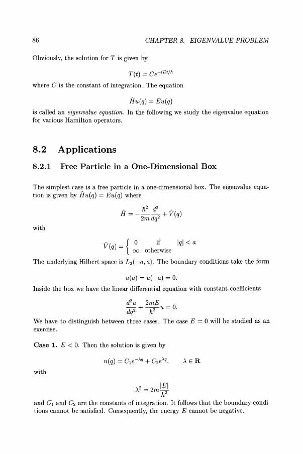
86 CHAPTER 8. EIGENVALUE PROBLEM
Obviously, the solution for T is given by
T(t) = Ce-iEt/ h
where C is the constant of integration. The equation
Hu(q) = Eu(q)
is called an eigenvalue equation. In the following we study the eigenvalue equation for various Hamilton operators.
8.2 Applications
8.2.1 Free Particle in a One-Dimensional Box
The simplest case is a free particle in a one-dimensional box. The eigenvalue equation is given by Hu(q) = Eu(q) where
A n?cP A
H = - 2m dq2 + V(q)
with
A { 0 if Iql < a V ( q) = 00 otherwise
The underlying Hilbert space is L2 ( -a, a). The boundary conditions take the form
u(a) = u( -a) = O.
Inside the box we have the linear differential equation with constant coefficients
cPu 2mE dq2 +yu=O.
We have to distinguish between three cases. The case E = 0 will be studied as an exercise.
Case 1. E < O. Then the solution is given by
with
).2 = 2ml~1 n
). E R
and C1 and C2 are the constants of integration. It follows that the boundary conditions cannot be satisfied. Consequently, the energy E cannot be negative.
8.2. APPLICATIONS 87
Case 2. E > O. We set
It follows that
The general solution is given by
u(q) = C1 sin(kq) + C2 cos(kq)
where C1 and C2 are the constants of integration. Then the boundary conditions u(a) = u( -a) = 0 can be satisfied.
Let C2 = 0 (sine-solution). Imposing the boundary conditions yield
and
ka = n7r, nE N
( ) 1. (n7rq) u - (q) = -sm -n vfci a
n27r2;,,2 E(-)=--
n 2ma2
where E~-) are the eigenvalues of the eigenfunctions u~-).
Let C1 = 0 (cosine-solution). Imposing the boundary conditions yield
and
1 ka = (n - -)7r,
2 nEN
u(+)(q) = - cos 2 1 ([n - l]7rq) n vfci a
( 1)2 2~2 E(+) = n - 2 7r fb
n 2ma2
where E~+) are the eigenvalues of the eigenfunctions u~+). The (±) signs refer to the even (odd) property under the reflection q -+ -q (see chapter 10).
We find that
(u(+) u(+)} = 8 m 'n mn, (u(-) u(-)} = 8
m 'n mn
88 CHAPTER 8. EIGENVALUE PROBLEM
The set
B := {u~+), u~-): n EN}
forms an orthonormal basis in the Hilbert space L 2 ( -a, a). The ground state energy (lowest eigenvalue) is given by
2,,2 E~ +) = _7r_It_.
8ma2
Let v be a linear combination of the orthonormal basis given above, i.e.
00
v(q) = 2)A~+)u~+)(q) + A~-)u~-)(q)l· n=l
Then we find
(v,iJV) == (p) = 0
where
A(+) .= (v u(+)) n· 'n' A~-) := (v, ut))
and p := -ihd/dq is the momentum operator.
The classical counterpart is as follows. We have a free particle
p2 H(p,q) = 2m
in a one-dimensional box together with elastic reflection at q = a and q = -a. The equation of motion inside the box takes the form
dp = 0 dt '
dq p dt m
The particle moves with constant velocity and is elastically reflected at the boundary. The time average over a cycle (-a --+ +a --+ -a) is given by
(p)cl = f p(t) dt = o.
Therefore (p)cl = (P)qm.
8.2. APPLICATIONS
8.2.2 Rotator
For the rotator the Hamilton function is given by
1 p2 H(p"" </J) = -2 ~ mr
or
H(P",,</J) = ~ where () is the mass moment of inertia, i. e. () = mr2. We notice that
o ~ </J < 21f,
After quantization
'Ii a P", --t -z -a</J
we obtain the Schrodinger equation
. a1/J Ii 2 f)21/J zliFt = - 2() a</J2 .
The underlying Hilbert space is L2(81) where
S1 := {(x, y): x2 + y2 = I}
The separation ansatz
1/J(</J, t) = T(t)u(</J)
gives the eigenvalue equation
The boundary condition is u(</J + 21f) = u(</J).
On inspection we find the solution
unit circle.
U(</J) = C exp(iv'2()E(</J + </Jo)/Ii)
89
where C and </Jo are the constant of integration. We set </Jo = O. Imposing the boundary condition gives
or
90 CHAPTER 8. EIGENVALUE PROBLEM
where n E Z. It follows that
1i2n2 E=En=--
2(}
where n E Z. The first few eigenvalues are given by
The eigenfunctions are
Eo 0
E1 1i2
E_1 = 2(}
E2 21i2
E_2=O'
1 . A.
u n (¢) = /"i"Cetn'l' v21f
where n E Z. Obviously, the functions Un are orthogonal and form an orthonormal basis in the Hilbert space L2(S1).
An application is as follows. Molecules with two atoms H2 , O2 can be considered as a rotator (first approximation) with
Then
and
() ~ 10-24 • 10-16 g cm2 = 10-40 g cm2
he A = - = 10-3 cm = 1OJ.t
tlE ultra red
where A denotes the wave length.
An extension of the Hamilton operator is as follows. A rigid rotator with the moment of inertia () and an electrical moment p is rotating in a plane. A homogeneous electric field E in q direction is applied. Then the Hamilton operator takes the form
" 1i2 cP H = --- - pEcos¢ 2(} d¢2
with the underlying Hilbert space L2 (S1 ). As mentioned above an orthonormal basis in L2(S1) is given by
B.2. APPLICATIONS 91
nE Z}. Since the eigenvalues of fI cannot be calculated exactly, we have to calculate the matrix representation Hmn of fI with the basis given above. Obviously the matrix (Hmn) is infinite-dimensional. This infinite dimensional matrix is a self-adjoint unbounded operator in 12(N). To calculate the lowest eigenvalues approximately we have to truncate the infinite dimensional matrix to a finite dimensional matrix. Of course first one has to show that the spectrum of the Hamilton operator is discrete.
The calculation is as follows. First we note that
eit/> + e-it/> cos¢;= 2 .
Consequently, the calculation of the matrix elements is as follows
where m, n E Z. We introduce the order 0,1, -1,2, -2, ....
We have to truncate the infinite dimensional matrix and calculate the eigenvalues of the finite dimensional matrix numerically.
When we introduce a magnetic field 1i the Hamilton operator takes the form
A 1i2 rf2 d H = - 2() d¢;2 + iJL1i d¢; - pc cos¢;
Then the matrix representation of the Hamilton operator is given by
92 CHAPTER 8. EIGENVALUE PROBLEM
If the electric field £ is equal to zero, then the lowest eigenvalues are given by
n 0 Eo =0
li2 n 1 El = - - J1.1l 2()
n = -1 . ".2
E-l = 2() + J1.1l.
8.2.3 Free Particle in a Bounded n-Dimensional Region
We consider a free particle in an n-dimensional bounded region R. The boundary of the region R is denoted by 8R. In the classical case the particle is reflected elastically at the boundary 8R. The Hamilton function inside the region R is given by
2
H(p,q) = :m where
The quantization rules are
Pk -+ -ili~ 8qk
p% -+ _li2~ 8q~
li2 n 82 li2 --L-2=--~·
2m k=l 8qk 2m
Then the eigenvalue equation is given by
or
We set
li2 --~u=Eu
2m
2Em -~u=7u.
8.2. APPLICATIONS 93
Therefore
-Au = AU.
This equation can also be considered as a Helmholtz equation. Let R be the region with a piecewise smooth boundary of 8R. Then the boundary conditions are
u(q E 8R) = O.
This is the so-called Dirichlet boundary condition. This is the corresponding boundary condition to the classical case. We recall that the boundary condition in the classical case is that the particle is elastically reflected at the boundary 8R. Obviously the underlying Hilbert space is L2(R).
This partial differential equation is intimately related to time-dependent equations such as the wave equation, but also has a connection with potential theory (Stakgold [58]).
For most values of the complex parameter A, the only solution of the system is the function u == 0 in R. Any exceptional number A, for which the system has a nontrivial solution u, is known as an eigenvalue. The corresponding nontrivial solution u is an eigenfunction. If to some eigenvalue A, there correspond two or more independent eigenfunctions, we say that A is a degenerate eigenvalue. If there is only one independent eigenfunction corresponding· to A - that is, if every eigenfunction corresponding to A can be written in the form CUi, where Ui is a fixed function and c is an arbitrary constant - then we call A a simple eigenvalue.
To find some properties of the eigenvalues and eigenfunctions, we recall that the inner product in the Hilbert space L 2 (R) is given by
(u, v) := f uv dq. R
Consequently, the norm is given by
All functions u under consideration are supposed to belong to the Hilbert space L2 (R)i that is, lIull < 00. We recall that u and v are orthogonal if (u, v) = O. If we mUltiply the differential equation -Au = AU by u and integrate over R, we find
Allull 2 = - f uAudq. R
Using the first form of Green's theorem and taking the boundary condition on u into account, we have
94 CHAPTER 8. EIGENVALUE PROBLEM
Allul1 2 = f (grad u . grad u) dq = f Igrad ul2 dq R R
where
8u 8u 8u 8u gradu . gradu = -8 -8 + ... + -8 -8 .
ql ql qn qn
The right side is nonnegative and
lIuli =I 0
if u is an eigenfunction. Consequently A is real, nonnegative. Moreover
implies
gradu == 0
in R, that is, u is constant in R. Since u must vanish on 8R, the constant is 0, so that u is not an eigenfunction. Thus we have shown that all eigenvalues are real and positive.
Next let u and v be eigenfunctions corresponding, respectively, to the eigenvalues A and f..L, where A =I f..L. Since A and f..L are real, we have
-~v = jiv = f..LV
and
u(q E 8R) = 0, v(q E 8R) = O.
Multiplying the first differential equation by v, the second by u, subtract, and integrating over R, yields
(A-f..L)(U,V) = f(u~v-v~u)dq. R
From Green's theorem and the boundary conditions on u and v, we find
(A - f..L)(u,v) = 0
and, since A =I f..L,
(u,v) = o. Therefore we find that eigenfunctions corresponding to different eigenvalues are orthogonal. Furthermore, one can prove that the normalized eigenfunctions of -~u = AU form an orthonormal basis over R.
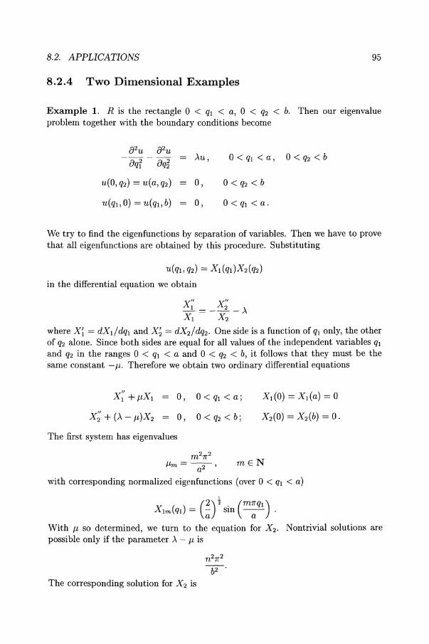
8.2. APPLICATIONS 95
8.2.4 Two Dimensional Examples
Example 1. R is the rectangle 0 < ql < a, 0 < q2 < b. Then our eigenvalue problem together with the boundary conditions become
(Pu 82u AU, 0< ql < a, 0<q2<b - 8q? - 8q~
u(O, q2) = u(a, q2) 0, 0<q2<b
U(ql' 0) = U(ql' b) = 0, 0< ql < a.
We try to find the eigenfunctions by separation of variables. Then we have to prove that all eigenfunctions are obtained by this procedure. Substituting
u(qt, q2) = Xl (qt}X2(q2)
in the differential equation we obtain
X~ X; -=---A Xl X 2
where Xf = dXt/dql and X~ = dX2/dq2' One side is a function of ql only, the other of q2 alone. Since both sides are equal for all values of the independent variables ql and q2 in the ranges 0 < ql < a and 0 < q2 < b, it follows that they must be the same constant -IL. Therefore we obtain two ordinary differential equations
0, 0 < ql < a; Xl(O) = Xl (a) = 0
X 2(0) = X2(b) = O.
The first system has eigenvalues
mEN
with corresponding normalized eigenfunctions (over 0 < ql < a)
X1m(ql) = G) t sin (m:ql) .
With IL so determined, we turn to the equation for X 2 • Nontrivial solutions are possible only if the parameter A - IL is
The corresponding solution for X 2 is
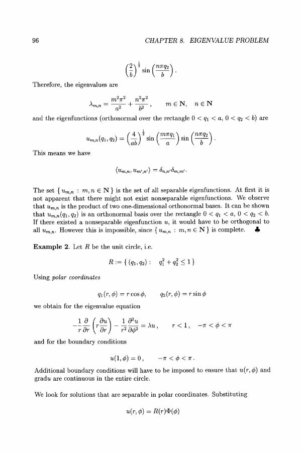
96 CHAPTER 8. EIGENVALUE PROBLEM
(~)! . (n7rq2 ) b sm b .
Therefore, the eigenvalues are
mEN, nEN
and the eigenfunctions (orthonormal over the rectangle 0 < ql < a, 0 < q2 < b) are
Um,n(ql, q2) = (~)! sin (m:q1 ) sin C:q2 ) .
This means we have
The set {um,n : m, n EN} is the set of all separable eigenfunctions. At first it is not apparent that there might not exist nonseparable eigenfunctions. We observe that um,n is the product of two one-dimensional orthonormal bases. It can be shown that Um,n(Ql, Q2) is an orthonormal basis over the rectangle 0 < Ql < a, 0 < Q2 < b. If there existed a nonseparable eigenfunction u, it would have to be orthogonal to all um,n. However this is impossible, since {um,n : m, n EN} is complete. "
Example 2. Let R be the unit circle, i.e.
Using polar coordinates
we obtain for the eigenvalue equation
_!~ (/JU) _ ~ 82u _ AU r 8r 8r r2 8cjJ2 - , r < 1 , -7r < ¢ < 7r
and for the boundary conditions
u(l,¢) = 0, -7r < ¢ < 7r.
Additional boundary conditions will have to be imposed to ensure that u(r, ¢) and gradu are continuous in the entire circle.
We look for solutions that are separable in polar coordinates. Substituting
u(r, ¢) = R(r)cI>(¢)
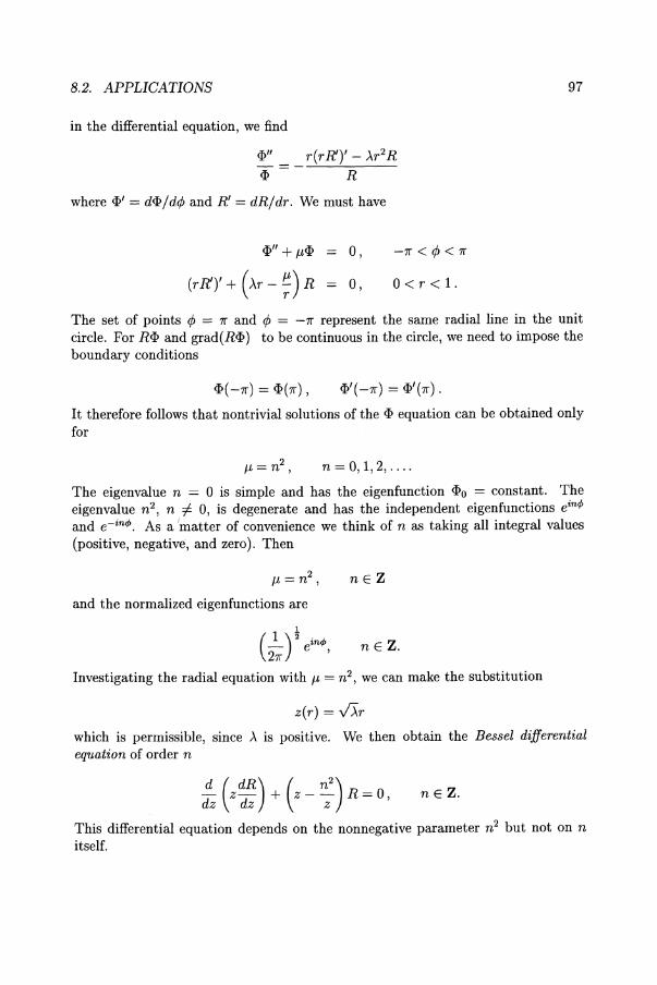
8.2. APPLICATIONS 97
in the differential equation, we find
=
where <1>' = d<l> / dtP and R' = dR/ dr. We must have
<1>" + JL<I> = 0, -7r < tP < 7r
0, O<r<1.
The set of points tP = 7r and tP = -7r represent the same radial line in the unit circle. For R<I> and grad(R<I» to be continuous in the circle, we need to impose the boundary conditions
It therefore follows that nontrivial solutions of the <I> equation can be obtained only for
n = 0,1,2, ....
The eigenvalue n = 0 is simple and has the eigenfunction <1>0 = constant. The eigenvalue n2 , n =1= 0, is degenerate and has the independent eigenfunctions eint/> and e-int/>. As a 'matter of convenience we think of n as taking all integral values (positive, negative, and zero). Then
JL = n2 ,
and the normalized eigenfunctions are
nEZ
nE Z.
Investigating the radial equation with JL = n2 , we can make the substitution
z(r) = v>'r which is permissible, since A is positive. We then obtain the Bessel differential equation of order n
~ (zdR) + (z _ n2) R = 0, dz dz z
nE Z.
This differential equation depends on the nonnegative parameter n2 but not on n itself.
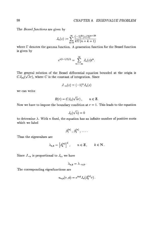
98 CHAPTER 8. EIGENVALUE PROBLEM
The Bessel functions are given by
00 (_1)k(z/2)n+2k In(z) := E k!r(n + k + 1)
where r denotes the gamma function. A generation function for the Bessel function is given by
00
ez(t-l/t)/2 = "" J. ( )tn L..J n Z . n=-oo
The general solution of the Bessel differential equation bounded at the origin is C Jlnl ( .J>.r), where C is the constant of integration. Since
we can write
nE Z.
Now we have to impose the boundary condition at r = 1. This leads to the equation
to determine A. With n fixed, the equation has an infinite number of positive roots which we label
/3~n) , /3~n) , •...
Thus the eigenvalues are
[ (n)]2 An,k = 13k , nE Z, kEN.
Since J_n is proportional to I n , we have
An,k = A_n,k.
The corresponding eigenfunctions are
8.2. APPLICATIONS
The functions I n ((3in )r) with n fixed, form an orthogonal set with weight rover
O<r<1.
We also derived the normalization integral
1 J rJ~(j3in)r)dr = ~ [J~(j3in»)r . o
Therefore, the set of functions
is orthonormal over the unit circle, that is,
m =I- n or j =I- k m = nand j = k
99
We can show that the set Un,k is complete and that there are no nonseparable eigenfunctions.
Remark. Another system which can be solved exactly is the free particle in a regular triangle (Steeb [61]). Here, too, we can make a separation ansatz. For more complicated domains this is not possible in general. The most famous example is the free particle (in two dimensions) confined in a stadium (or racetrack) boundary. This system is well understood in the classical case. The particle is reflected elastically at the boundary. It is chaotic (nearby trajectories separate exponentially) for all nonzero values of the aspect ratio 'Y = a/ R (a being the half-length of the straight side, R being the radius of the semicircle). The degree of chaos increases from zero at 'Y = 0 (the circle) to a flat maximum near 'Y = 1. The quantum problem for the free particle is the Helmholtz equation. The boundary condition at the stadium wall is u(8R) = o. This problem must be solved numerically. The Hamilton operator is invariant under reflection in x and y. For further reading we refer to McDonald and Kaufman [40j. In particular, they studied the distribution of eigenvalue spacings for the eigenfunctions of odd-odd parity.
100 CHAPTER 8. EIGENVALUE PROBLEM
Exercises. (1) Study the case E = 0 for the free particle in a one-dimensional box.
(2) Consider a particle in the Hilbert space L2([0, a] x [0, b] x [0, c]), where a, b, c> O. Find the eigenvalues and eigenfunctions. Are the eigenvalues degenerate?
(3) Consider the Schrodinger equation (11, = 1)
8 A
i 8t 'IjJ(t) = H(t)'IjJ(t)
with the time-dependent Hamilton operator H(t) defined on the Hilbert space 1l(t) = L2[0, f(t)] as
A 82
H(t) = - 8x2
with Dirichlet boundary conditions describing the elastic collisions with the wall 'IjJ{0, t) = 'IjJ{f{t), t) = O. We assume that f(t) is smooth, positive and periodic with period T,
f{t) = f{t + T),
df(O)/dt = 0,
f{O) = f{T) = 1
df(T)/dt = O.
Consider the evolution equation
8 A
i 8t U{t) = H(t)U(t)
and the map W{{t) : L2{0, 1) --t L2[0,f{t)]
[W{t)-l f](x) := f{t) 1/2 exp ( -~f{t) d~~) X2) f(f{t)x)
and
U{t) = W{t)U{t)
where U is some unitary operator defined on the fixed Hilbert space L2(0, 1). Show that
i! U(t) = (W{t)-l H{t)W(t) - iW(ttl :t W(t)) U(t)
and
. 8 - 1 (A 1 3 d2f(t) 2) -z at U(t) = f(t)2 Ho + 4{f(t)) ---;[i2x U{t)
where Ho = -82 /8x2 with Dirichlet boundary conditions 'IjJ(0) = 'IjJ(1) = O.
Chapter 9
Spin Matrices and Kronecker Product
In this chapter we study spin systems. In Pauli's nonrelativistic theory of spin certain spin wave functions, vectors, or spinor functions - along with spin operators, or matrices - are introduced to facilitate computation. We define
and
It) .- (~)
It) .- (~)
spin-up vector
spin-down vector
( 0 -i) Cly := i 0 '
The matrices Clx , Cly, Clz , are called the Pauli spin matrices. Let I be the 2 x 2 unit matrix. We find the following relationships. After squaring the spin matrices, we have
Cl; = I, Cl; = I, Cl; = I. Since the squares of the spin matrices are the 2 x 2 unit matrix, their eigenvalues are ±l. The anticommutators are given by
where 0 is the 2 x 2 zero matrix.
101
W.-H. Steeb, Hilbert Spaces, Wavelets, Generalised Functions and Modern Quantum Mechanics© Kluwer Academic Publishers 1998
102 CHAPTER 9. SPIN MATRICES AND KRONECKER PRODUCT
Summarizing these results we have
0i(Jj + 0jOi = 215ij I
where i and j may independently be x, y, or z and l5ij is the Kronecker delta. The matrices I, OX, Oy and Oz form an orthogonal basis in the Hilbert space M2. This means every 2 x 2 matrix can be written as
M = CxOx + cyOy + CzOz + clI
where cx, cY ' c z , Cl E C. Another orthonormal basis (standard basis) is given by
The trace of a matrix is the sum of the diagonal terms. For all three Pauli spin matrices the trace is zero. The Pauli spin matrices are self-adjoint operators (hermitian matrices) and therefore have real eigenvalues. The commutators are given by
These three relationships may be combined in a single equation u x u = 2iu, where x denotes the vector product and u = (ox, 0Y' oz? We define
These are the spin-flip operators. We define
The two matrices are projection matrices. As mentioned above the four matrices o ±, A± form an orthonormal basis in the Hilbert space M2.
Let us now study the action of spin matrices on spin vectors. A vector u E C 2 can be written as
where Ul, U2 E C. We find the following relations
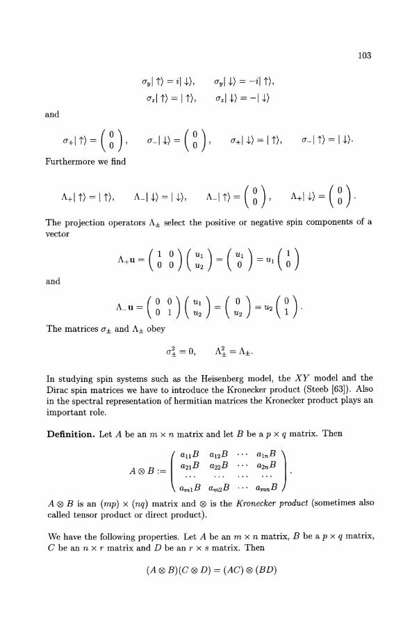
and
Furthermore we find
ayl t) = il-l-),
azl t) = It),
ayl-l-) = -il t),
azl-l-) = -1-1-)
a_I t) = 1-1-)·
103
The projection operators A± select the positive or negative spin components of a vector
and
The matrices a± and A± obey
2 - 0 a±- ,
In studying spin systems such as the Heisenberg model, the XY model and the Dirac spin matrices we have to introduce the Kronecker product (Steeb [63]). Also in the spectral representation of hermitian matrices the Kronecker product plays an important role.
Definition. Let A be an m x n matrix and let B be a p x q matrix. Then
( anB a12B ... a1nB)
A B a21B a22B ... a2nB .0.. ._ ~ .- . ... ... .., ...
amlB am2B ... amnB
A ® B is an (mp) x (nq) matrix and ® is the Kronecker product (sometimes also called tensor product or direct product).
We have the following properties. Let A be an m x n matrix, B be a p x q matrix, C be an n x r matrix and D be an r x s matrix. Then
(A ® B)(C ® D) = (AC) ® (BD)
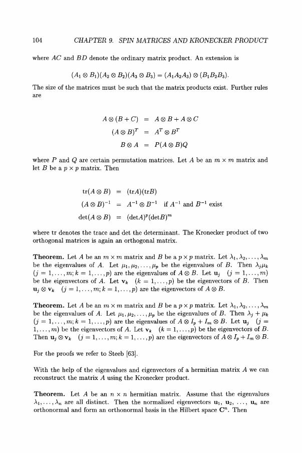
104 CHAPTER 9. SPIN MATRICES AND KRONECKER PRODUCT
where AC and BD denote the ordinary matrix product. An extension is
The size of the matrices must be such that the matrix products exist. Further rules are
A® (B+C)
(A® B)T
B®A P(A®B)Q
where P and Q are certain permutation matrices. Let A be an m x m matrix and let B be a p x p matrix. Then
tr(A ® B)
(A® B)-l
det(A® B)
(trA)(trB)
A-I ® B-1 if A-I and B-1 exist
(detA)P(detB)m
where tr denotes the trace and det the determinant. The Kronecker product of two orthogonal matrices is again an orthogonal matrix.
Theorem. Let A be an m x m matrix and B be a p x p matrix. Let AI, A2"'" Am be the eigenvalues of A. Let J.Ll, J.L2, . .. , J.Lp be the eigenvalues of B. Then AjJ.Lk (j = 1, ... ,m;k = 1, ... ,p) are the eigenvalues of A®B. Let Uj (j = 1, ... ,m) be the eigenvectors of A. Let Vk (k = 1, ... ,p) be the eigenvectors of B. Then Uj ® Vk (j = 1, ... , m; k = 1, ... ,p) are the eigenvectors of A ® B.
Theorem. Let A be an m x m matrix and B be a p x p matrix. Let AI, A2, ... , Am be the eigenvalues of A. Let J.Ll. J.L2, ... , J.Lp be the eigenvalues of B. Then Aj + J.Lk (j = 1, ... , m; k = 1, ... ,p) are the eigenvalues of A ® Ip + 1m ® B. Let Uj (j = 1, ... , m) be the eigenvectors of A. Let Vk (k = 1, ... ,p) be the eigenvectors of B. Then Uj ® Vk (j = 1, ... , m; k = 1, ... ,p) are the eigenvectors of A ® Ip + 1m ® B.
For the proofs we refer to Steeb [63].
With the help of the eigenvalues and eigenvectors of a hermitian matrix A we can reconstruct the matrix A using the Kronecker product.
Theorem. Let A be an n x n hermitian matrix. Assume that the eigenvalues AI, . .. , An are all distinct. Then the normalized eigenvectors Ub U2, ... , Un are orthonormal and form an orthonormal basis in the Hilbert space en. Then
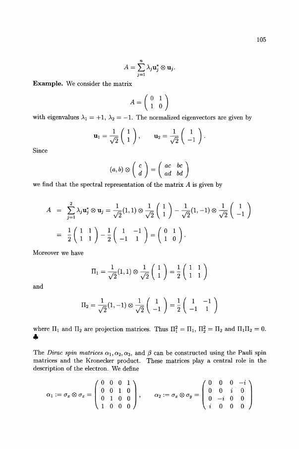
n
A = LAjUj ®Uj. j=l
Example. We consider the matrix
A=(~ ~) with eigenvalues Al = +1, A2 = -1. The normalized eigenvectors are given by
Since
( e) (ae be) (a, b) ® d = ad bd
we find that the spectral representation of the matrix A is given by
A tAjU;®Uj = ~(1,1)® ~( ~) - ~(1,-1)®~ (~1)
= ~ (~ ~) - ~ (~1 ~1) = (~ ~). Moreover we have
and
105
where III and II2 are projection matrices. Thus IIi = Ill, m = II2 and II1II2 = o. "-The Dirac spin matrices (};l, (};2, (};3, and f3 can be constructed using the Pauli spin matrices and the Kronecker product. These matrices playa central role in the description of the electron. We define
01) 1 0 o 0 ' o 0
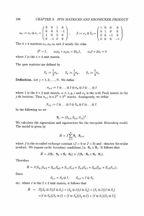
106 CHAPTER 9. SPIN MATRICES AND KRONECKER PRODUCT
a, ,~ u. ® u, ~ (! 0 1
~1 ) fi~ u.®I, ~ U 0 0
~) 0 0 1 0 0 0 o ' 0 -1
-1 0 0 0 0 -1
The 4 x 4 matrices 0:1,0:2,0:3 and /3 satisfy the rules
/32 = 1, O:i/3 + /3O:i = 0
where 1 is the 4 x 4 unit matrix.
The spin matrices are defined by
Definition. Let j = 1,2, ... , N. We define
aa,j := 1 ® ... ® 1 ® aa ® 1 ® ... ® 1
where 1 is the 2 x 2 unit matrix, 0: = X, y, z and aa is the o:-th Pauli matrix in the j-th location. Thus aa,j is a 2N x 2N matrix. Analogously, we define
Sa,j := 1 ® ... ® 1 ® Sa ® 1 ® ... ® 1.
In the following we set
Sj := (S""j, Sy,j, Sz,jl.
We calculate the eigenvalues and eigenvectors for the two-point Heisenberg model. The model is given by
2
iI = JL Sj . Sj+1
j=l where J is the so-called exchange constant (J > 0 or J < 0) and· denotes the scalar product. We impose cyclic boundary conditions, i.e. S3 == Sl. It follows that
Therefore
Since S""l = S'" ® I, S",,2 = 1 ® S'"
etc. where 1 is the 2 x 2 unit matrix, it follows that
iI = J[(S", ® 1)(1 ® Sx) + (Sy ® I) (I ® Sy) + (Sz ® 1)(1 ® Sz)
+(1 ® Sx)(Sx ® 1) + (1 ® Sy)(Sy ® 1) + (I ® Sz)(Sz ® 1)].
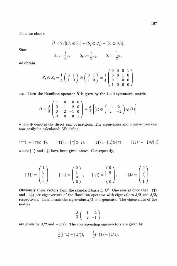
107 Thus we obtain
Since
we obtain
1 ( 0 Sx Ql; Sx = 4" 1 01) 1 0 o 0 o 0
etc .. Then the Hamilton operator iI is given by the 4 x 4 symmetric matrix
( 1 0 0 0) A J 0 -1 2 0 J -1 2
H = 2" 0 2 -1 0 == 2" [(1) E9 (2 -1) E9 (1)] o 0 0 1
where E9 denotes the direct sum of matrices. The eigenvalues and eigenvectors can now easily be calculated. We define
1 tt) := 1 t)Ql;1 t), 1 tt) := 1 t)Ql;1 t), 1 H) := 1 t)Ql;1 t), 1 U) := 1 t)Ql;1 t)
where I t) and 1 t) have been given above. Consequently,
Obviously these vectors form the standard basis in C 4 . One sees at once that 1 tt) and 1 tt) are eigenvectors of the Hamilton operator with eigenvalues J /2 and J /2, respectively. This means the eigenvalue J /2 is degenerate. The eigenvalues of the matrix
~ (-; -i) are given by J /2 and -3J /2. The corresponding eigenvectors are given by
1 2"(1 H) + 1 H)), ~(I H) -I tt))·
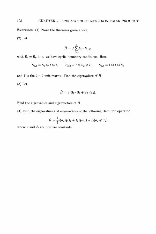
108 CHAPTER 9. SPIN MATRICES AND KRONECKER PRODUCT
Exercises. (1) Prove the theorems given above.
(2) Let
3
if = J:E Sj· Sj+1
;=1 with S4 = Sl, i. e. we have cyclic boundary conditions. Here
Sx,2 = 1 ® Sx ® 1,
and 1 is the 2 x 2 unit matrix. Find the eigenvalues of H.
(3) Let
Find the eigenvalues and eigenvectors of H.
(4) Find the eigenvalues and eigenvectors of the following Hamilton operator
A 1 H = 2f(O"z ® h + 12 ® O"z) - ~(O"x ® O"x)
where f and ~ are positive constants.
Chapter 10
Parity and Group Theory
Finite group theory plays an important role in quantum mechanics (Miller [42], Ludwig and Falter [38]). In this chapter we give an application of group theory in quantum mechanics using the parity operator. First we introduce the definition of a group and describe some of its properties. Then we give an application in quantum mechanics.
A group is an abstract mathematical entity which expresses the intuitive concept of symmetry.
Definition. A group G is a set of objects {g, h, k, ... } (not necessarily countable) together with a binary operation which associates with any ordered pair of elements g, h in G a third element gh. The binary operation (called group multiplication) is subject to the following requirements:
(1) There exists an element e in G called the identity element such that ge = eg = 9 for all 9 E G. (2) For every 9 E G there exists in G an inverse element g-l such that
gg-l = g-lg = e.
(3) Associative law. The identity
(gh)k = g(hk)
is satisfied for all g, h, kEG.
Thus, any set together with a binary operation which satisfies conditions (1)-(3) is called a group. If gh = hg we say that the elements 9 and h commute. If all elements of G commute then G is a commutative or abelian group. If G has a finite number of elements it has finite order n(G), where n(G) is the number of elements. Otherwise, G has infinite order.
109
W.-H. Steeb, Hilbert Spaces, Wavelets, Generalised Functions and Modern Quantum Mechanics© Kluwer Academic Publishers 1998
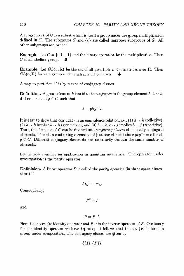
110 CHAPTER 10. PARITY AND GROUP THEORY
A subgroup H of G is a subset which is itself a group under the group multiplication defined in G. The subgroups G and {e} are called improper subgroups of G. All other subgroups are proper.
Example. Let G = {+ 1, -1} and the binary operation be the multiplication. Then G is an abelian group. ,.
Example. Let GL(n, R) be the set of all invertible n x n matrices over R. Then GL(n, R) forms a group under matrix multiplication. ,.
A way to partition G is by means of conjugacy classes.
Definition. A group element h is said to be conjugate to the group element k, h I'V k, if there exists agE G such that
It is easy to show that conjugacy is an equivalence relation, i.e., (1) h I'V h (reflexive), (2) h I'V k implies k I'V h (symmetric), and (3) h I'V k, k I'V j implies h I'V j (transitive). Thus, the elements of G can be divided into conjugacy classes of mutually conjugate elements. The class containing e consists of just one element since geg- 1 = e for all 9 E G. Different conjugacy classes do not necessarily contain the same number of elements.
Let us now consider an application in quantum mechanics. The operator under investigation is the parity operator.
Definition. A linear operator P is called the parity operator (in three space dimensions) if
Pq: = -q.
Consequently,
p2 =1
and
P= p-l.
Here 1 denotes the identity operator and p-l is the inverse operator of P. Obviously for the identity operator we have 1 q := q. It follows that the set {P, J} forms a group under composition. The conjugacy classes are given by
{{I}, {P}}.
111
Let Op be the corresponding operator which acts on functions.
Definition.
Since
p=p-l
it follows that Opu(q) : = u( -q).
Remark. The operator Op acts upon the coordinate q and not on the argument of u. This means. Let Rand P be two operators for which the inverse exists. Then
since
Therefore
Theorem. The eigenvalues of Op are given by ±l.
Proof. Since Opu( q) = '\u( q) we obtain
and Oppu(q) = '\Opu(q) = ,\2U(q).
Since P P = I it follows that
OJu(q) = ,\2u(q) =} u(q) = ,\2u(q).
Since u( q) i- 0 we find
,\2 = 1 =} ,\ = ±l.
Consequently the eigenvalues of the operator Op are {I, -I}. •
In the following we restrict ourselves to the one-dimensional case. Let
H = Hkin + V(q)
be a Hamilton operator in one space dimension. Let us calculate [Op, H]. We find
112 CHAPTER 10. PARlTY AND GROUP THEORY
[Op, H]U(q)
Op --- + V(q) U(q) - --- + V(q) U(-q) [( /i2 d2 )] ( /i2 ~ )
2mdq2 2mdq2
/i2 d2 A /i2 d2
A
---u(-q) + V(-q)u(-q) + --u(-q) - V(q)u(-q) 2mdq2 2mdq2
(V(-q) - V(q))u(-q).
If
V(-q) = v(q)
then
[Op, If]u(q) = 0
or
[Op, If] = o.
This means Op commutes with If if V(q) = V( -q). Examples of potentials V with V(q) = V( -q) are
and
Theorem. Let
A { 0 V(q) = 00
V(q) = cosq
-a~q~a
elsewhere
A /i2 d2 A
H=---+V(q) 2mdq2
with V(q) = V( -q). If u is an eigenfunction of If, then Opu is an eigenfunction of If with the same eigenvalue.
Proof. Since Ifu = Eu we obtain
113
::::} OpHu = OpEu
::::} HOpu = EOpu
::::} H(Opu) = E(Opu)
::::} Hu(-q) Eu(-q) . • Definition. A function u is called an even function if u(q) = u( -q). A function is called an odd function if u(q) = -u( -q).
Theorem. Assume that [Op, H] = O. Let 'ljJ(t = 0) be an even function. Then the wave function 'ljJ(t) remains an even function.
Proof.
ir/N = H'ljJ at
Remark. The same holds for odd functions.
Theorem. An arbitrary function u can always be written as a sum of an even and an odd function.
Proof. Using the identity
1 1 u(q) == 2[u(q) + u( -q)] + 2[u(q) - u( -q)]
we find that u(q) + u( -q) is an even function and u(q) - u( -q) is an odd function .
• We now introduce the character table and the corresponding projection operators. To find the character table we need the irreducible (matrix) representations of the finite group {P, I} and the conjugacy classes. The conjugacy classes have been given above.
Definition. Let G be a finite group. Let GL(n, C) be the set of all n x n invertible matrices over C. The mapping f: G -+ GL(n, C) is a homomorphism if
for all gl, g2 E G.
It follows that
114 CHAPTER 10. PARITY AND GROUP THEORY
f(e) = I
where e is the unit element in the group G and I is the n x n unit matrix.
Definition. A homomorphism f : G ---+ GL(n, C) is said to be an isomorphism if f is bijective.
Definition. Let G be a finite group. An n-dimensional matrix representation of G is a homomorphism T: 9 ---+ T(g) of G into GL(n, C), where GL(n, C) denotes the set of all invertible n x n matrices over C.
Let T be a matrix representation of a finite group G acting on the complex linear space V.
Definition. A subspace W of V is invariant under T if
T(g)w E W
for every 9 E G, w E W.
Definition. The representation T is reducible if there is a proper subspace W of V which is invariant under T. Otherwise, T is irreducible.
In the present case with G = {P, I} we have the irreducible one-dimensional representations (i.e. representation by 1 x 1 matrices).
(i) f(P) = 1
(ii) f(P) -1
f(1) = 1
f(1) = 1
Obviously, these representations are irreducible. We recall that the classes of the group {P, I} are {I} and {P}.
Theorem. The number of conjugacy classes is equal to the number of nonequivalent irreducible representations.
For the proof we refer to Miller [42].
The characters of a given class in different irreducible representations are unique and distinct from those of any other class. The character table is a square table since number of conjugacy classes = number of irreducible representations. The table displays the (trace) of the nonequivalent irreducible representations for the conjugacy classes. Therefore in our example the character table is given by
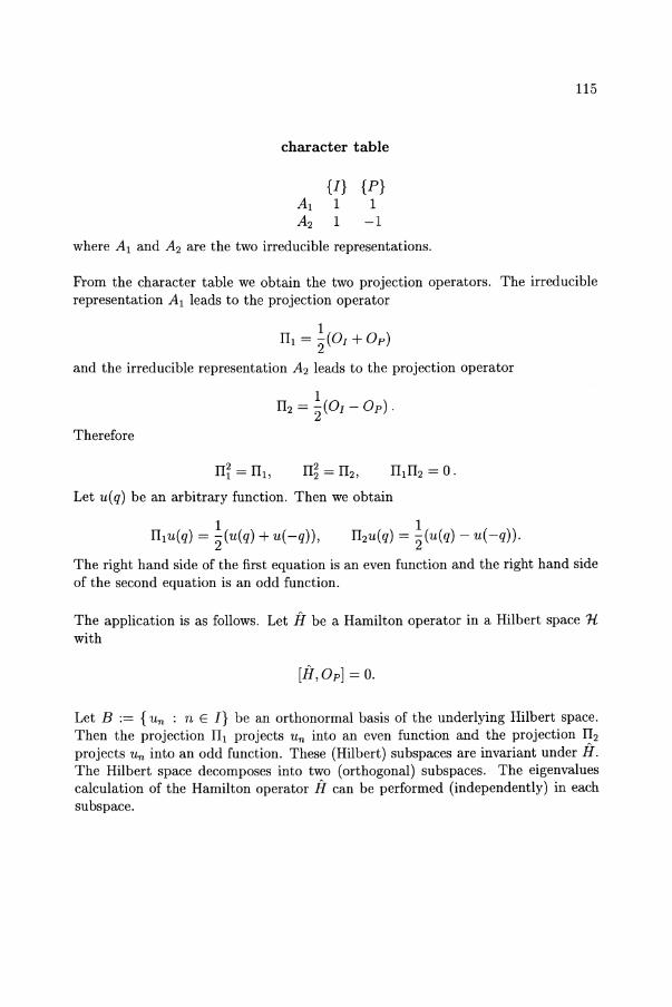
character table
{I} {P} AlII A2 1 -1
where Al and A2 are the two irreducible representations.
115
From the character table we obtain the two projection operators. The irreducible representation Al leads to the projection operator
1 III = 2"(O[ + Op)
and the irreducible representation A2 leads to the projection operator
Therefore
Let u(q) be an arbitrary function. Then we obtain
1 II2u(q) = 2" (u(q) - u(-q)).
The right hand side of the first equation is an even function and the right hand side of the second equation is an odd function.
The application is as follows. Let H be a Hamilton operator in a Hilbert space 'Ii with
[H,Op] = o.
Let B := {un : n E I} be an orthonormal basis of the underlying Hilbert space. Then the projection III projects Un into an even function and the projection II2 projects Un into an odd function. These (Hilbert) subspaces are invariant under H. The Hilbert space decomposes into two (orthogonal) subspaces. The eigenvalues calculation of the Hamilton operator H can be performed (independently) in each subspace.
116 CHAPTER 10. PARITY AND GROUP THEORY
Exercises. (1) Find all the symmetry operations on the square. These symmetry operations form a group. Show that this group is isomorphic to a subgroup of the permutation group. Hint. There are eight symmetry operations (including the identity operation).
(2) Show that all n x n unitary matrices form a group under matrix multiplication. A matrix is called unitary if U' = U- I .
(3) Let G be an Abelian group. Find the conjugacy classes.
(4) Find the eigenvalues of the projection operators III and II2·
(5) Show that
(6) Let III be a projection operator in the Hilbert space HI. Let II2 be a projection operator in a Hilbert space H 2 • Is
III 0 II2
a projection operator in the Hilbert space HI 0H2 ?
Chapter 11
Uncertainty Relation
In the chapter about Fourier and wavelet transforms we saw that all functions, including windows, obey the uncertainty principle, which states that sharp localizations in time and in frequency are mutually exclusive. Roughly speaking, if a nonzero function 9 of time is small outside a time-interval of length T and its Fourier transform is small outside a frequency band of width n, then an inequality of the type nT 2': c must hold for some positive constant c ~ 1. The precise value of c depends on how the widths T and n of the signal in time and frequency are measured. In this chapter we discuss the uncertainty relation (Prugovecki [47], Constantinescu and Magyari [15]) in quantum mechanics. In particular we study the uncertainty relation for the momentum and coordinate operators. First we discuss the commutation relation of unbounded operators (Collatz [14]).
There is a general theorem according to which the basic operators of quantum mechanics cannot all be bounded.
Theorem. If all iterated operators Qm (m = 0,1,2, ... ) exist then the operator relation
PQ-QP=aI
where a # ° is a real or complex number and I the identity operator, cannot be satisfied by two bounded operators, P, Q in a normed space.
Proof. It is reasonable to assume that the iterated operators Qm (m = 0,1,2, ... ) are meaningful. From PQ - QP = aI it follows that P and Q can neither be the null operator nor a constant. Therefore
IIPI! # 0, IIQII # 0.
Furthermore from this equation we find by induction that
117
W.-H. Steeb, Hilbert Spaces, Wavelets, Generalised Functions and Modern Quantum Mechanics© Kluwer Academic Publishers 1998
118 CHAPTER 11. UNCERTAINTY RELATION
For n = 1, PQn - Qn P = anQn-l is certainly true. It follows then that
anQ,,-lQ + QnaI = a(n + l)Qn
which completes the induction. We assume now P and Q to be bounded operators with the norms IIPII and IIQII. Taking norms on both sides of PQn_Qnp = anQn-l for n = 1,2,3, ... we find
Let N be an integer with
Two cases are now possible:
IIPQn _ Qnpil ::; IIPllllQnl1 + IIQnllllPl1
211P111IQnli ::; 21IPIIIIQn-1111IQII·
2 N > ~IIPIIIIQII.
Case 1. IIQN-111 =1= O. This results in a contradiction for n = N.
Case 2. IIQN-111 = O. Since
for all n = 1,2,3, ... , we find
IIQN-2 11 = 0, IIQN-3 11 = 0, ... , IIQ111 = 0
which is again a contradiction. •
Remark. In particular there are no two finite matrices P, Q which satisfy PQ-QP = aI, where a =1= o. This also follows from the fact that
tr[P,Q] = 0
and tr( aI) = an, where P and Q are arbitrary n x n matrices and I is the n x n unit matrix.
Remark. In the commutation relation
pq- qp = -in!
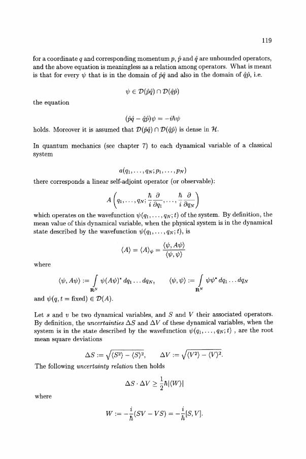
119
for a coordinate q and corresponding momentum p, p and q are unbounded operators, and the above equation is meaningless as a relation among operators. What is meant is that for every 'Ij; that is in the domain of pq and also in the domain of qp, i.e.
'Ij; E D(pq) n D(qp)
the equation
(prj - qp)'Ij; = -ih'lj;
holds. Moreover it is assumed that D(prj) n D(qp) is dense in 1l.
In quantum mechanics (see chapter 7) to each dynamical variable of a classical system
a(ql, ... ,qNiPl,.·· ,PN)
there corresponds a linear self-adjoint operator (or observable):
A(qb ... ,qNi~aa '···'~aa) l ql Z qN
which operates on the wavefunction 'Ij;(ql' ... ,qNi t) of the system. By definition, the mean value of this dynamical variable, when the physical system is in the dynamical state described by the wavefunction 'Ij;(ql' ... ,qNi t), is
(A) = (A) = ('Ij;, A'Ij;) t/J ('Ij;,'Ij;)
where
('Ij;, A'Ij;) := J 'Ij;(A'Ij;)* dql . .. dqN, ('Ij;, 'Ij;):= J 'Ij;'Ij;* dql ... dqN RN RN
and 'Ij;(q, t = fixed) E D(A).
Let s and v be two dynamical variables, and S and V their associated operators. By definition, the uncertainties b.S and b. V of these dynamical variables, when the system is in the state described by the wavefunction 'Ij;(ql' ... ,qNi t) , are the root mean square deviations
The following uncertainty relation then holds
b.S· b.V ~ ~hl(W)1 where
i i W:= --(SV - VS) = --[S, V].
h h
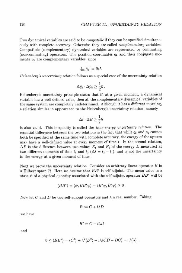
120 CHAPTER 11. UNCERTAINTY RELATION
Two dynamical variables are said to be compatible if they can be specified simultaneously with complete accuracy. Otherwise they are called complementary variables. Compatible (complementary) dynamical variables are represented by commuting (noncommuting) operators. The position coordinates qk and their conjugate momenta Pk are complementary variables, since
[qk,Pk] = in!.
Heisenberg's uncertainty relation follows as a special case of the uncertainty relation
tlijk . tlPk ~ ~ 11, •
Heisenberg's uncertainty principle states that if, at a given moment, a dynamical variable has a well-defined value, then all the complementary dynamical variables of the same system are completely undetermined. Although it has a different meaning, a relation similar in appearance to the Heisenberg's uncertainty relation, namely
tlt . tlE > ~n -2 is also valid. This inequality is called the time-energy uncertainty relation. The essential difference between the two relations is the fact that while qk and Pk cannot both be specified at the same time with complete accuracy, the energy of the system may have a well-defined value at every moment of time t. In the second relation, tlE is the difference between two values El and E2 of the energy E measured at two different moments of time it and t2 (tlt = t2 - t 1), and is not the uncertainty in the energy at a given moment of time.
N ext we prove the uncertainty relation. Consider an arbitrary linear operator B in a Hilbert space 11.. Here we assume that BB' is self-adjoint. The mean value in a state 'l{J of a physical quantity associated with the self-adjoint operator BB' will be
(BB*) = ('l{J, BB*'l{J) = (B*'l{J, B*'l{J) ~ o.
Now let C and D be two self-adjoint operators and .x a real number. Taking
B:= C+i.xD
we have
B* = C - i.xD
and
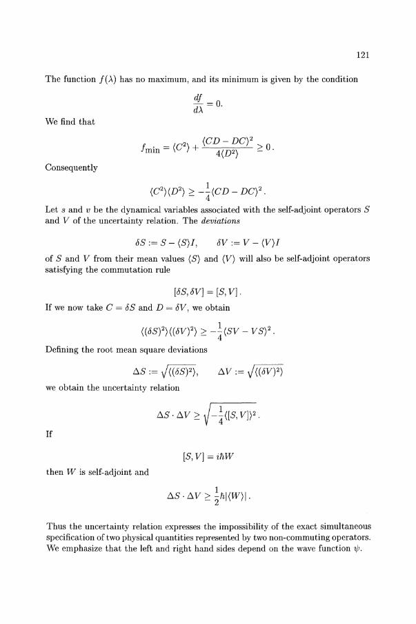
121
The function f(>.) has no maximum, and its minimum is given by the condition
df d>' = O.
We find that
2 (CD - DC)2 f min = (C ) + 4(D2) ~ 0 .
Consequently
(C2)(D2) ~ -~(CD - DC)2.
Let s and v be the dynamical variables associated with the self-adjoint operators 8 and V of the uncertainty relation. The deviations
68 := 8 - (8)1, 6V:= V - (V)1
of 8 and V from their mean values (8) and (V) will also be self-adjoint operators satisfying the commutation rule
[68,6V) = [8, V).
If we now take C = 68 and D = 6V, we obtain
((68)2)((6V)2) ~ -~(8V - V8)2.
Defining the root mean square deviations
!J.8 := )((68)2),
we obtain the uncertainty relation
If
[8, V) = iliW
then W is self-adjoint and
!J.8· !J. V ~ ~lil (W) I.
Thus the uncertainty relation expresses the impossibility of the exact simultaneous specification of two physical quantities represented by two non-commuting operators. We emphasize that the left and right hand sides depend on the wave function 'IjJ.
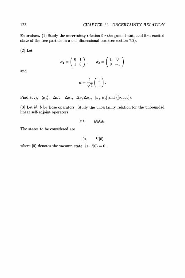
122 CHAPTER 11. UNCERTAINTY RELATION
Exercises. (1) Study the uncertainty relation for the ground state and first excited state of the free particle in a one-dimensional box (see section 7.2).
(2) Let
and
(3) Let bt , b be Bose operators. Study the uncertainty relation for the unbounded linear self-adjoint operators
The states to be considered are
ID), btlD)
where ID) denotes the vacuum state, i.e. biD) = D.
Chapter 12
Harmonic Oscillator
12.1 Classical Case The Hamilton function of the harmonic oscillator in one space dimension is given by
The first term describes the kinetic energy and the second the potential energy. The mass m and the frequency w are constants. The Hamilton equations of motion take the form
It follows that
dq P dt m'
dp 2 dt = -mw q.
~q 2 dt2 +w q = O.
The general solution of this equation is given by q(t) = C cos w(t - to), where C and to are the constants of integration. The general solution can also be written as
where C1 and C2 are constants of integration. Inserting the initial conditions
q(t = 0) = qo,
yields
p(t = 0) = Po
Po C2 =-·
mw
123
W.-H. Steeb, Hilbert Spaces, Wavelets, Generalised Functions and Modern Quantum Mechanics© Kluwer Academic Publishers 1998
124
It follows that
Let
CHAPTER 12. HARMONIC OSCILLATOR
q(t) = qocoswt+ ~sinwt. mw
p2 Hkin = 2m'
Using the solution we find
Hkin (t) = ~mw2C2 sin2 wet - to), Vet) = ~mw2C2 cos2 wet - to)
H(t) = ~mw2C2 = E 2 .
Obviously the kinetic part and the potential part of the Hamilton function depend on time, whereas the Hamilton function does not depend on time, i.e. the Hamilton function is a constant of motion.
In classical mechanics we can introduce the so-called time-average value.
Definition. Let J be a bounded continuous function that oscillates more or less irregularly for all t E [0,00). The time average of function J is defined as
T
(j(t)) : = lim -T1 / J(t) dt. T--+oo
o
If the function J is periodic, i.e. ,
J(t) = J(t + 27f) W
T = 27f W
then the definition simplifies to
~
(j(t)) := ~ JW J(t) dt. 27f
For the harmonic oscillator we find
(q(t)) = 0,
(q2(t)) = ~C2,
(Hkin(t)) = ~mw2C2,
o
(p(t)) = 0
(p2(t)) = ~m2w2C2 2
(V(t)) = ~mw2C2. The time-average values will be compared later with the expectation values from quantum mechanics.
12.2. QUANTUM CASE
12.2 Quantum Case
The eigenvalue equation H u = Eu is given by
(-!{~ + ~mw2q2) u(q) = Eu(q). 2m dq2 2
The underlying Hilbert space is L2(R). To simplify the problem, we introduce
qO:= fh, y-:;;;;; \ '= 2E -1 A. liw ' u(~(q)) = u(q)
125
where qo has the dimension of a length. Then the eigenvalue equation takes the form
(:;2 -e + ). + 1) u(~) = O. Since u E V(H) c L2(R) we make the ansatz
1 ~2 u(O = AH(~)e-2 for the wave function, where the normalization constant A is determined later. Then
(:;2 -2~ :~ + -\) H(~) = O.
To solve this linear second order differential equation we make the power series ansatz
m=O
Inserting the power series ansatz into the differential equation yields
2m-). a - a
m+2 - (m + 1)( m + 2) m
(recursion relation). The solution is given by
H(~) 00 ~2m
ao J;o (-),)(4 -).) ... (4m - 4 -).) (2m)!
00 em+1 + al J;o (2 - -\)(6 - ).) ... (4m - 2 - -\) (2m + I)!
where ao and al are the constants of integration. Now we have to impose the boundary condition. Since u E V(H) c L2(R) we have
u(q) -+ 0 as iqi -+ 00.
126 CHAPTER 12. HARMONIC OSCILLATOR
If A =I- {O, 2, 4, ... }, then
for m» 1.
Then we obtain the asymptotic behaviour
Consequently
A = 2n, n =0,1,2,3, ....
Then the series truncates and the boundary condition can be satisfied. Inserting this into into A = 2E/(fiw) - 1 leads to the eigenvalues
1 En = (n + 2)fiw n = 0,1,2,3, ...
The functions H(~) are polynomials with
We normalize
Therefore
al 0 for A = 0,4,8, 12, .. .
ao 0 for A = 2,6, 10, .. .
( -l)%n! !!.I 2 .
2(-1)~n! n-11
2 .
al = 0 for n = 0,2,4,6, ...
aO = 0 for n = 1,3,5, ...
~ (_1)%-m(2~)2m n! L ( ) for n = 0, 2, 4, 6, ...
m=O ~ - m !(2m)!
n;-i (-1)~-m(2~)2m+l Hn(~) = n! L () for n= 1,3,5, ...
m=O n;l - m !(2m + 1)!
The functions Hn(~) are the so-called Hermite polynomials.
To summarize. The Hermite polynomials are solutions of the linear second order differential equation
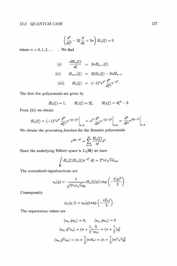
12.2. QUANTUM CASE
where n = 0,1,2, . . . . We find
( i)
( ii)
( iii)
The first few polynomials are given by
Ho(~) = 1,
From (iii) we obtain
Hn(~) = (_1) nee2 dnne-<e-tJ21 = ee' d: e-<e-tl21 = d:e2et-t21 . d~ t=o dt t=o dt t=o
We obtain the generating function for the Hermite polynomials
Since the underlying Hilbert space is L2(R) we have
J Hn(~)Hm(~)e-e2 d~ = 2n n!v'7f6nm .
R
The normalized eigenfunctions are
Consequently
( ) ( iEnt) Wn q, t) = un(q exp -T . The expectation values are
127
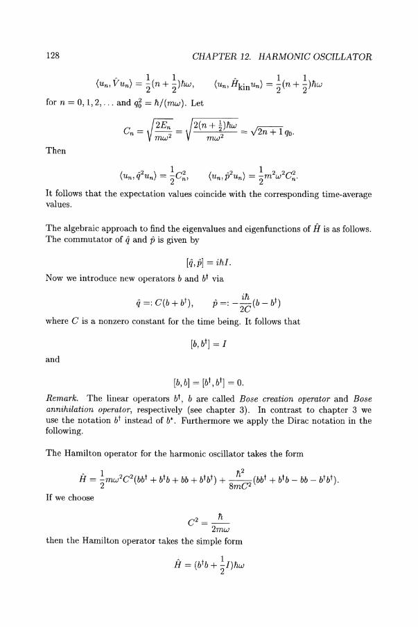
128 CHAPTER 12. HARMONIC OSCILLATOR
All (un, VUn) = "2(n + "2)liw,
for n = 0,1,2, ... and q3 = fi/(mw). Let
c - J2En -n - mw2 -
Then
( A2 ) 1 C 2 un,q Un ="2 n'
2(n+~)liw ~ ---'---"2'::'-- = v 2n + 1 qo·
mw
It follows that the expectation values coincide with the corresponding time-average values.
The algebraic approach to find the eigenvalues and eigenfunctions of iI is as follows. The commutator of ij and p is given by
[ij,p] = iii!.
Now we introduce new operators band bt via
where C is a nonzero constant for the time being. It follows that
and
[b, b] = [bt , btl = o. Remark. The linear operators bt , b are called Bose creation operator and Bose annihilation operator, respectively (see chapter 3). In contrast to chapter 3 we use the notation bt instead of b*. Furthermore we apply the Dirac notation in the following.
The Hamilton operator for the harmonic oscillator takes the form
If we choose
C2 = _fi_ 2mw
then the Hamilton operator takes the simple form
A t 1 H = (b b+ "2I)liw
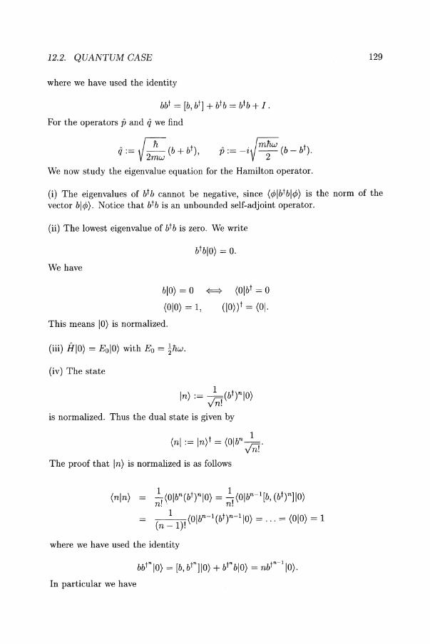
12.2. QUANTUM CASE 129
where we have used the identity
bbt = [b, btl + btb = btb + I. For the operators p and ij we find
We now study the eigenvalue equation for the Hamilton operator.
(i) The eigenvalues of btb cannot be negative, since (¢>Ibtbl¢» is the norm of the vector bl¢». Notice that btb is an unbounded self-adjoint operator.
(ii) The lowest eigenvalue of btb is zero. We write
We have
blO) = 0
(010) = 1,
{:==> (OW = 0
(IO»)t = (01.
This means 10) is normalized.
(iii) HIO) = EoIO) with Eo = ~1iw.
(iv) The state
In) := _l_(bt tIO) vnr is normalized. Thus the dual state is given by
The proof that In) is normalized is as follows
(nln) = ~/Olbn(bt)nIO) = ~(Olbn-l[b, (bt)n]IO) n!' n!
(n ~ I)! (0Ibn-1(bt)n-lI0) = ... = (010) = 1
where we have used the identity
In particular we have
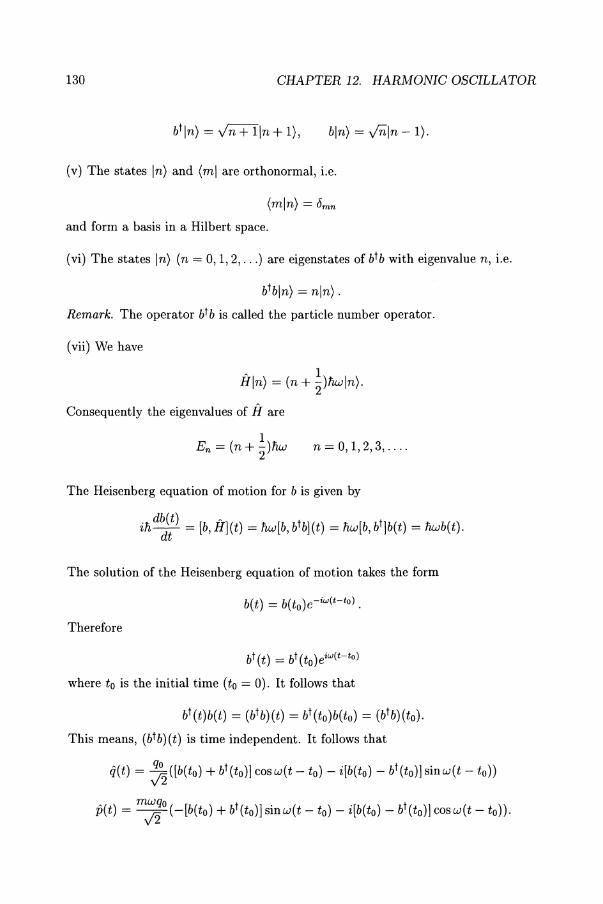
130 CHAPTER 12. HARMONIC OSCILLATOR
bin} = v'nln - I}.
(v) The states In} and (ml are orthonormal, i.e.
(min) = omn and form a basis in a Hilbert space.
(vi) The states In) (n = 0,1,2, ... ) are eigenstates of btb with eigenvalue n, i.e.
btbln} = nln} .
Remark. The operator btb is called the particle number operator.
(vii) We have
A 1 Hln} = (n + 2)1iwln).
Consequently the eigenvalues of Hare
n = 0,1,2,3, ....
The Heisenberg equation of motion for b is given by
in d~~) = [b, H](t) = nw[b, btb](t) = 1iw[b, bt]b(t) = nWb(t).
The solution of the Heisenberg equation of motion takes the form
b(t) = b(to)e-iw(t-to) .
Therefore
bt(t) = bt(to)eiw(t-to)
where to is the initial time (to = 0). It follows that
bt(t)b(t) = (btb)(t) = bt(to)b(to) = (btb)(to).
This means, (btb)(t) is time independent. It follows that
q(t) = ~([b(to) + bt(to)] cosw(t - to) - i[b(to) - bt(to)] sinw(t - to))
p(t) = ~o (-[b(to) + bt(to)] sinw(t - to) - i[b(to) - bt(to)] cosw(t - to)).
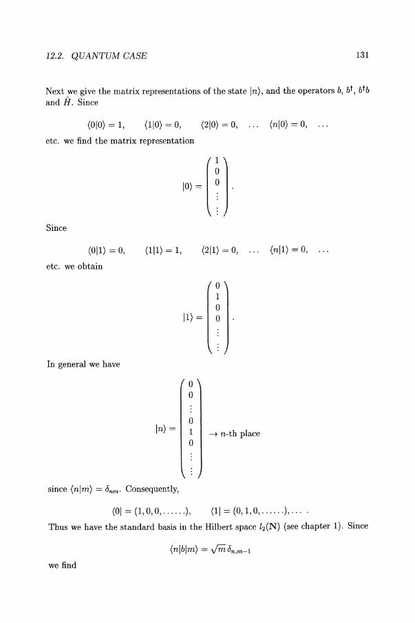
12.2. QUANTUM CASE 131
Next we give the matrix representations of the state In), and the operators b, bt , btb and iI. Since
(010) = 1, (110) = 0, (210) = 0,
etc. we find the matrix representation
Since
(0il) = 0, (111) = 1,
etc. we obtain
In general we have
In) =
since (nlm) = 8nm . Consequently,
1°) =
1
° o
(211) = 0,
o 1 o
11) = 0
0 0
0 1 --+ n-th place 0
(nIO) = 0,
(nil) = 0,
(01 = (1,0,0, ...... ), (11 = (0,1,0, ...... ), ... .
Thus we have the standard basis in the Hilbert space l2(N) (see chapter 1). Since
(nlblm) = Viii 8n ,m-l
we find
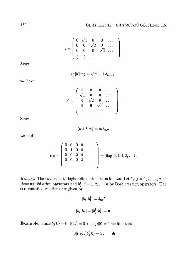
132 CHAPTER 12. HARMONIC OSCILLATOR
b ~ (~ y'I 0 0
) 0 v'2 0 0 0 J3
Since
(nlbtlm) = v'm + 1bn,m+1
we have
000 y'I 0 0
bt = 0 v'2 0 o 0 J3
Since
(nlbtblm) = mOn,m
we find
0 0 0 0 0 1 0 0
btb = 0 0 2 0 = diag(O, 1,2,3, ... ) . 0 0 0 3
Remark. The extension to higher dimensions is as follows. Let bj , j = 1,2, ... , n be Bose annihilation operators and b;, j = 1,2, ... , n be Bose creation operators. The commutation relations are given by
Example. Since bjlO) = 0, (Olb; = 0 and (010) = 1 we find that
(0Iblb2blb~10) = 1. ..
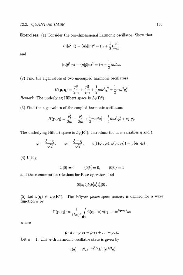
12.2. QUANTUM CASE 133
Exercises. (1) Consider the one-dimensional harmonic oscillator. Show that
and
(2) Find the eigenvalues of two uncoupled harmonic oscillators
p2 p2 1 1 H(p q) = _1 + _2 + _mw2q2 + _mw2q2.
, 2m 2m 2 1 2 2
Remark. The underlying Hilbert space is L2 (R2 ).
(3) Find the eigenvalues of the coupled harmonic oscillators
The underlying Hilbert space is L 2(R2 ). Introduce the new variables 'T} and ~
(4) Using
bjlO} = 0, (Olb) = 0, (010) = 1
and the commutation relations for Bose operators find
(5) Let u(q) E L2(Rn). The Wigner phase space density is defined for a wave function u by
f(p, q) := (1i~)n / u(q + s)u(q - s)e2ip.s/lids Rn
where
p. s := P1S1 + P2S2 + ... + PnSn
Let n = 1. The n-th harmonic oscillator state is given by
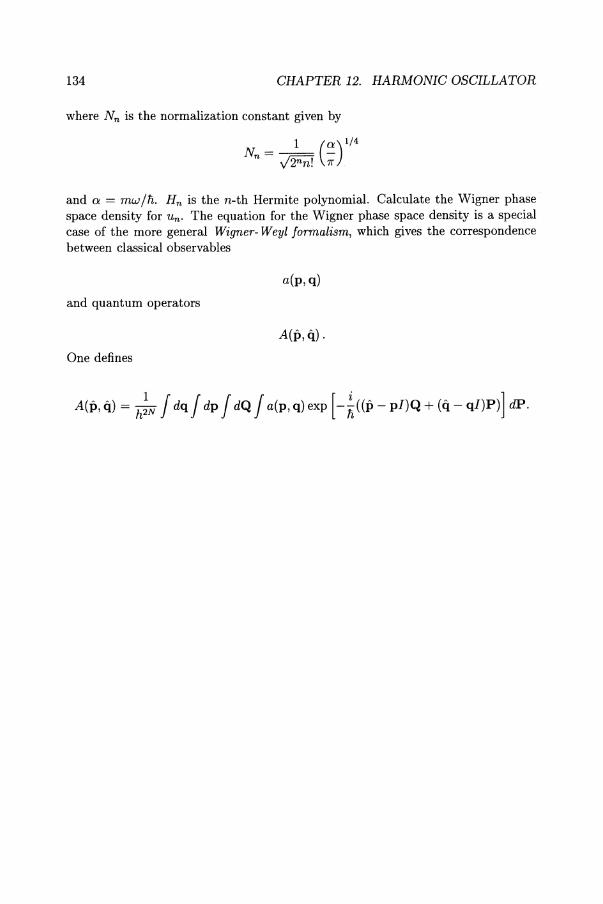
134 CHAPTER 12. HARMONIC OSCILLATOR
where Nn is the normalization constant given by
1 (a)1/4 Nn = J2nn! -:;
and a = mw/h. Hn is the n-th Hermite polynomial. Calculate the Wigner phase space density for Un. The equation for the Wigner phase space density is a special case of the more general Wigner- Weyl formalism, which gives the correspondence between classical observables
a(p, q)
and quantum operators
A(p, q).
One defines
A(p, q) = h;N J dq J dp J dQ J a(p, q) exp [-k((p - pI)Q + (q - qI)P)] dP.
Chapter 13
Coherent and Squeezed States
In chapter 12 we introduced the Bose operators band bt. In this chapter we study the spectrum of b. This leads to the so-called coherent states (Louisell [37]). We adopt the Dirac notation. Coherent states are applied to a wide variety of physical problems (Klauder and Skagerstam [32], Kowalski and Steeb [33]).
Definition. Let b be a Bose annihilation operator. Consider the eigenvalue problem
blJi) = 13113).
The state 113) is called a Bose coherent state.
To solve the eigenvalue problem (1) we use the number representation In), where
(bt)n In):= -10)
v'nf and n = 0, 1,2, .... Therefore
bin) = v'nln - 1)
We apply the completeness relation of the number representation. This means we expand 113) with respect to In). We obtain
00 00
113) = L In)(nl13) == L c,.(13) In) n=O n=O
where
en(13) := (nl13)·
135
W.-H. Steeb, Hilbert Spaces, Wavelets, Generalised Functions and Modern Quantum Mechanics© Kluwer Academic Publishers 1998
136 CHAPTER 13. COHERENT AND SQUEEZED STATES
If we insert this equation into the eigenvalue equation bl,8) = ,BI,8) we obtain
00 00
L cn(!3)vnl n - 1) = L ,8cn(,8)vnln). n=l n=O
The first sum goes from 1 to 00 since the term n = 0 vanishes. We can therefore shift indices and put n --+ n + 1. It follows that
00 00
L Cn+l (,8) In + lin) = L ,8cn(,8)vnl n). n=O n=O
If we apply the dual state (ml and use
we obtain the linear difference equation
On inspection we see that
etc .. Consequently
Therefore
Cn+l (,8) Vn+l = ,8cn(,8).
,8 -co JI ,8 ,82
v'2C1 = y'2T CO
,83 J3T CO
,8n cn (,8) = ClCO·
vn!
00 ,8n 1,8) = Co ~ Vnfln).
We normalize 1,8) to determine co. From the condition
(,81,8) = 1
we obtain
where we used that
137
It follows that
where (3 E C.
As an example we consider the displaced harmonic oscillator
iI = btb - 'Y(bt + b)
where l' is a real number. We want to find the eigenvalues and eigenfunctions of iI. The eigenvalue equation is given by
We set
Introducing
we obtain from the eigenvalue equation that
or
This is the harmonic oscillator eigenvalue problem. Since
1 -t n l4>n) = VnT(b) 14>0)
with bl4>o) = 0 we find the eigenvalues
En = n - 1'2
and the ground state from the equation
138 CHAPTER 13. COHERENT AND SQUEEZED STATES
Thus
bl1Pg(bt )) = 'Y11Pg(bt )). Consequently, the ground state is a coherent state, i.e.
l1Pg(bt)) = e-'Y2/2e'YbtIO).
For the excited state we obtain
Next we introduce so-called squeezed states. They are a generalization of coherent states.
Definition. A squeezed state is the eigenfunction IJLII,B) of the linear operator
B := JLb + IIbt
where JL, II are complex numbers. This means
where
so that the commutation relation
[B,Bt] = I is satisfied. It is easy to see that condition [B, Bt] = I implies IJLI2 - 11112 = 1.
An ideal squeezed state is obtained from the vacuum state 10) by operation with the squeezing operator
S( () = exp G(b2 - ~(bt2) followed by operation with the displacement operation D(,B):
IJLII,B) = D(,B)S(() 10)
where
( rei8
IJLI2 cosh21rl
11112 = sinh2lrl.
A squeezed state satisfies the following relations
1 -2r -e 4
1 2r -e 4
139
These equations show that a squeezed state satisfies the minimum uncertainty product and has a different amount of noise in the two quadrature components. Here the complex amplitude axis ((31, (32) is rotated by () /2 so that (32 represent the minor and major axes of the error ellipse. Furthermore these equations indicate that part of the mode energy Ivl2 is consumed to reduce one of the quadrature noises.
Remark. Let V be a finite dimensional linear space. Consider the linear operators eL et ... , e~ and el,~,"" en acting in this linear space. We assume that these operators satisfy the anti-commutation relation
where
[A, Bl+ := AB + BA.
The operators are called Fermi creation and annihilation operators. One easily finds that
(e)? = 0 j = 1,2, ... ,no
This is the Pauli principle. The vacuum state 10) is defined as
CjIO) = 0,
for j = 1,2, ... , n. Thus we find that
(Olc; = 0,
(010) = 1
j = 1,2, ... ,n.
140 CHAPTER 13. COHERENT AND SQUEEZED STATES
Exercises. (1) Show that
(2) Show that for coherent states the Heisenberg uncertainty relation takes the form
Remark. The coherent states minimalize the Heisenberg uncertainty relations. In this sense they are the closest to the classical states.
(3) Let 111) and I,) be coherent states. Show that
(111,) = e-(h'1 2 +1.81 2 )/2+')',8.
Remark. This means that the coherent states are not orthogonal.
(4) Show that
Remark. The coherent states become approximately orthogonal as ir- 1112 increases.
(5) Show that
J 111)(l1l d; = I c
where I is the identity operator. The integration is over the whole complex plane. If we set
11 = x + iy = re i ¢
then
d211 = dxdy = rdrd¢J.
Remark. Consequently the coherent states form a complete set.
(6) Show that
00
L In)(nl = I. n=O
Chapter 14
Angular Momentum and Lie Algebras
In the classical case the angular momentum is given by
L:= r x p
where x denotes the cross product. The components of L are given by
Introducing the quantization
yields
.~ a Px -+ -znax '
L .=!!:. (y~ -z~) X· i az ay'
Furthermore we define
L± := Lx ± iLy .
.~ a P -+ -Zn
z az
Here it is convenient to introduce the notion of a Lie algebra. Lie algebras arise "in nature" as vector spaces of linear transformations endowed with a new operation which is in general neither commutative nor associative: [x, y] = xy - yx (where the operations on the right hand side are the usual ones). It is possible to describe this kind of system abstractly in a few axioms.
141
W.-H. Steeb, Hilbert Spaces, Wavelets, Generalised Functions and Modern Quantum Mechanics© Kluwer Academic Publishers 1998
142 CHAPTER 14. ANGULAR MOMENTUM AND LIE ALGEBRAS
Definition. A vector space L over a field F, with an operation L x L -+ L, denoted by (x, y) t-+ [x, y] and called the bracket or commutator of x and y, is called a Lie algebra over F if the following axioms are satisfied:
(L1) The bracket operation is bilinear.
(L2) [x, x] = 0 for all x in L.
(L3) [x, [y, zJ] + [y, [z, xJ] + [z, [x, yJ] = 0 (x, y, z, E L).
Axiom (L3) is called the Jacobi identity. Notice that (L1) and (L2), applied to [x + y, x + y] implyanticommutativity: (L2')
[x, y] = -[y, x].
Conversely, if charF =I- 2, it is clear that (L2') will imply (L2). In the following we have F = R or F = C. Thus charF =I- 2.
We say that two Lie algebras L, L' over F are isomorphic if there exists a vector space isomorphism ¢: L -+ L' satisfying
¢([x, yJ) = [¢(x), ¢(y)]
for all x, y in L (and the ¢ is called an isomorphism of Lie algebras). Similarly, it is obvious how to define the notion of a Lie subalgebra of L. A subspace K of L is called a subalgebra if [x, y] E K whenever x, y E K; in particular, K is a Lie algebra in its own right relative to the inherited operations. Note that any nonzero element x E L defines a one dimensional subalgebra, with trivial multiplication, because of (L2).
Definition. Let V and W be the differential operators (vector fields)
n 8 V:= LVj(r)~,
j=l vXj
where we have used the notation Xl, X2, X3 instead of x, y, z. Then the commutator of V and W is defined by
The operators Lx, Ly and Lz form a basis of a Lie algebra under the commutator. Show that
In classical mechanics Lx, Ly and L z form a basis of a Lie algebra under the Poisson bracket (see chapter 5). Are the Lie algebras isomorphic?
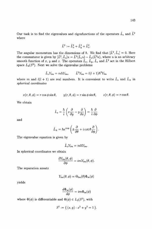
143
Our task is to find the eigenvalues and eigenfunctions of the operators Lz and L2 where
L2 := L; + L~ + L;.
The angular momentum has the dimensions of n. We find that [L2, Lzl = O. Here the commutator is given by [L2, Lzlu = L2(Lzu) - Lz(L2u), where u is an arbitrary smooth function of x, y and z. The operators Lx, Ly, Lz and L2 act in the Hilbert space L2(S2). Next we solve the eigenvalue problems
~2 2 L Yim = l(l + 1)1i Yim
where m and l(l + 1) are real numbers. It is convenient to write Land L± in spherical coordinates
x(r,(},ify) = rcosifysin(}, y(r, (), ify) = r sin ify sin (),
We obtain
and
L± = lie±it/> ( ± :() + i cot () :ify) .
The eigenvalue equation is given by
LzYim = mnYim·
In spherical coordinates we obtain
8Yim((}, ify) =. y, (() A.) 8ify zm 1m ,'/'.
The separation ansatz
yields
d<Pm(ify) =. n. (A.) dify zm'i'm '/'
where <p(ify) is differentiable and <p(ify) E L2(S1), with
S1 := { (x, y) : x2 + y2 = I}.
z(r,(},ify) = r cos ().
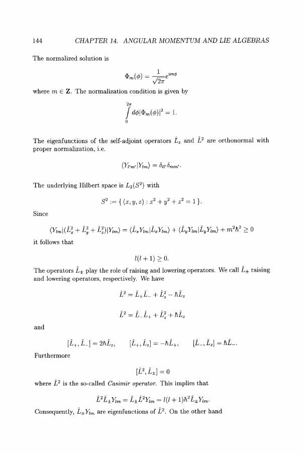
144 CHAPTER 14. ANGULAR MOMENTUM AND LIE ALGEBRAS
The normalized solution is
<I>m(¢) = ~eim4J
where m E Z. The normalization condition is given by
271"
J d¢l<I>m(¢W = l. o
The eigenfunctions of the self-adjoint operators Lz and L2 are orthonormal with proper normalization, i.e.
The underlying Hilbert space is L2(32) with
Since
S 2 .- { ( ). 2 2 2 - 1 } .- x, y, z . x + y + z - .
(Yiml(L; + L; + L;)I)'lm} = (LxYimILxYim) + (LyYimILyYim) + m 2h2 ~ 0
it follows that
l(l+l)~O.
The operators L± play the role of raising and lowering operators. We call L± raising and lowering operators, respectively. We have
and
Furthermore
[L2, L±J = 0
where L2 is the so-called Casimir operator. This implies that
'2' , '2 2' L L±Yim = L±L Yim = l(l + l)h L±Yim· Consequently, L± Yim are eigenfunctions of L2. On the other hand
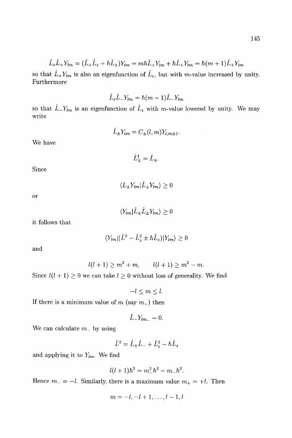
145
LJ.J+Yim = (L+Lz + hL+)Yim = mhL+Yim + hL+Yim = h(m + l)L+Yim
so that L+Yim is also an eigenfunction of Lz, but with m-value increased by unity. Furthermore
LL-Yim = h(m - l)L-Yim
so that L-Yim is an eigenfunction of Lz with m-value lowered by unity. We may write
We have
Since
or
it follows that
and
l(l+1);:::m2+m, l(l + 1) ;::: m 2 - m.
Since l(l + 1) ;::: 0 we can take l ;::: 0 without loss of generality. We find
-l:::; m:::; l.
If there is a minimum value of m (say m_) then
We can calculate m_ by using
'2 " '2 ' L = L+L_ + Lz - hLz
and applying it to Yim. We find
l(l + 1)h2 = m~h2 - m_h2.
Hence m_ = -l. Similarly, there is a maximum value m+ = +l. Then
m = -l, -l + 1, ... ,l - 1, l
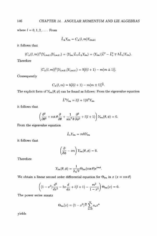
146 CHAPTER 14. ANGULAR MOMENTUM AND LIE ALGEBRAS
where l = 0, 1,2, .... From
it follows that
2 A A A2 A2 A IC±(l, m)1 (Y1,m±lIYl,m±l) = (YimI L'fL±Y1m) = (Yiml(L - Lz =F liLz)Y1m).
Therefore
Consequently
C±(l, m) = Ii[l(l + 1) - m(m ± I)]!.
The explicit form of Y1m(O, ¢) can be found as follows: From the eigenvalue equation
it follows that
From the eigenvalue equation
it follows that
Therefore
(:¢ - im) Y1m(O,¢) = o.
Y1m(O, ¢) = 1r,;;8Im(cosO)eim4>. 2y7r
We obtain a linear second order differential equation for 8 1m in x (x == cos 0)
The power series ansatz
00
8 1m (x) = (1 - X 2 )T L anxn
n=O
yields
147
(_1)l+m 2l + 1 (l- m)! !!!c 00 (2n)! (_1)nx2n-I-m e/m(x) = 21 -2-· (l+m)!(1-X2)2 E n! r(l-n+1){2n-l-m)!
where ao = 0 for l + m odd and al = 0 for l + m even, otherwise the solution would diverge for x 2 -t 1. Here r denotes the gamma function
00
r(n) := J e-xxn-ldx, o
n > O.
Moreover, l = 0,1,2,... . Therefore
(2l + 1) (l- m)! 2 !!!c 00 (2n)! (_1)nx2n-I-m 2 . (l + m)! (1 - x ) 2 E 7· (l - n)!(2n - l - m)!
or
e () = (_1)l+m 2l + 1. (l- m)!(1_ 2)T dl+m (1- 2)1 1m X 21l! 2 (l + m)! X dxl+m x.
To summarize. The spherical harmonics are given by
where
J Yi;"(O, ¢)Yl1ml(O, ¢) dn = 811'8mml 8 2
and dn = sin OdOd¢. The completeness relation is given by
00 +1
L L Ylm(O, ¢)Yi;"(IJ', ¢') sinO = 8(0 - O')8(¢ - ¢') I=Om=-1
where 8 denotes the delta function. The first few spherical harmonics are given by
148 CHAPTER 14. ANGULAR MOMENTUM AND LIE ALGEBRAS
Exercises. (1) Show that the Laplacian operator Ll in spherical coordinates is given by
Ll= - - r - +--- smB- +----1[8(28) 18(.8) 182 ] r2 8r 8r sin B 8B 8B sin 2 B 8(p
almost everywhere, i.e. with the exception of the z-axis, which is a set of zero Lebesgue measure.
(2) Show that the operators L+, L_ and Lz form a Lie algebra under the commutator.
(3) Show that the spherical harmonics l'lm can be written as
where
(_1)1 dl+lml R ( ) - --(1 _ 2)m/2 __ (1 _ 2)1 1m X - 21l! X dxl+lml x.
(4) Show that
where
cos e = cos B cos Bf + sin B sin B' cos (cjJ - cjJ') .
Chapter 15
Two-Body Bound State Problem
15.1 Introduction When a system consists of only two particles of different kinds, the states are represented by wave functions 'ljJ(rI, r2, t), in the six configuration space variables rl and r2. The underlying Hilbert space is L 2 (R6 ). Let
and
The eigenvalue equation takes the form
where, on physical grounds, only potentials depending on rl - r2 exclusively are considered. We introduce the invertible transformation
149
W.-H. Steeb, Hilbert Spaces, Wavelets, Generalised Functions and Modern Quantum Mechanics© Kluwer Academic Publishers 1998
150 CHAPTER 15. TWO-BODY BOUND STATE PROBLEM
where r is the relative position vector and R is the center of mass position vector. It follows that
where
82 82 82
DoR := 8X2 + 8y2 + 8Z2' R := (X, Y, Z)T
82 82 82
Do:= 8x2 + 8y2 + 8z2' r := (x, y, z)T
and
mlm2 M:= ml +m2, m·- _~c:....-
.- ml +m2
Here M denotes the total mass and m denotes the reduced mass.
If we make the separation ansatz
U(R, r) = uc(R)u(r)
we obtain the eigenvalue equations
and
( - :~ Do + V(r)) u(r) = Ebu(r)
where Ec + Eb = E. In the following we study this eigenvalue problem.
15.2 Spherical Oscillator The Hamilton operator is given by (Fliigge [22])
;,,2 1 fI := - 2m Do + "2mw2r2
where the Laplace operator Do expressed in spherical coordinates takes the form
Let
fIu = Eu
15.2. SPHERICAL OSCILLATOR 151
be the eigenvalue equation. The underlying Hilbert space is L 2 (R3 ). By the usual separation ansatz
1 u(r, 8, cp) = ;:Rt(r)Yi,m(8, cp)
we obtain the radial equation
The spherical harmonics have already been studied in chapter 14. For l = 0 this again turns out to be identical with the differential equation for the harmonic oscillator (see chapter 11). For l -I- 0 the centrifugal force described by the term
l(l + 1) ---r2
will drive the particle outwards so that we find different solutions. Now we introduce the abbreviations
mw r;:-.>',
k2 E -=-=:j.L. 2>' nw
Thus we can write the radial equation in the standard form
d2 Rl (k2 _ \ 2 2 _ l (l + 1)) R = 0 d 2 + /\r 2 t • r r
The behaviour of the solution at r = 0, determined by the centrifugal term, and its asymptotic behaviour, determined by the oscillator term >.r2 , suggest to write
Rt(r) = rl+le-~r2v(r).
The transformation of the dependent variable r
v(t(r)) = v(r)
leads to d2v 3 dv 1 3 1) _ t dt2 + ((l + 2) - t) dt - (2 (l + 2) - 2 j.L v = 0 .
This second order linear differential equation is the Kummer equation with the general solution
152 CHAPTER 15. TWO-BODY BOUND STATE PROBLEM
where Cl and C2 are the constants of integration and IFI denotes the confluent series which is defined by
fCc) 00 rea + n) z I Fl(a,C;Z):=r()L r ( ) ,. a n=O c+ n n.
Here f denotes the gamma function. At r = 0, the second part of the solution contradicts normalization so that C2 = O. This differs from the linear harmonic oscillator where no boundary condition exists at the origin. A confluent series behaves asymptotically at large positive values of its argument as
F ( ) r(c) z a-c 1 1 a,c;z -t f(a)e z .
Consequently,
Rz(r) ex: rl+le-~lr2 e"r\-(l+~+")
is exponentially divergent. The divergence cannot be avoided except by putting the parameter
with
nr = 0,1,2, ... ,
thus transforming the series into a polynomial of degree nr . Hence,
Thus the energy levels become
1 3 -(l + - - Jl) = -nr . 2 2
3 E = 1iw(2nr + l + 2) ; nr = 0,1,2, ....
The quantity nr is called the radial quantum number. The energy levels start with a zero-point energy of ~ 1iw corresponding to the three degrees of freedom of the problem and are equidistant, as with the linear oscillator
where
n:= 2nr + l. Thus we find that the complete eigenfunctions may be written as
15.3. HYDROGEN-LIKE ATOMS 153
where C has to be determined from the normalization condition. The eigenfunctions form an orthonormal basis in the Hilbert space L2(R3).
The energy levels are degenerate, except for the ground state n = 0, as, for even n, there are ~n+ 1 partitions of n and, for odd n, there are ~(n+ 1). Since l = 0, 1,2, ... we find that for each value of l, there are still 2l + 1 different values of m (ranging from -l to +l), the degeneracy is again increased by this factor.
15.3 Hydrogen-like Atoms
The Hamilton operator is given by
A fi,2 fi,2 Ze2
H = - --!:1N - -!:1e - ----;-----;-2mN 2me 47l'folre - rNI
where Z is the number of protons in the nucleus. The number of protons is equal to the number of electrons. The first term of the Hamilton operator describes the kinetic part of the nucleus, the second term the kinetic part of the electron and the third term the potential part. Here re is the position of the electron and rN is the position of the nucleus.
We introduce new coordinates Rand r as we did in section 15.1
where
M =me+mN.
It follows that the Schrodinger equation takes the form
( 1'1,2 fi,2 Ze2 a)
--!:1R - -!:1r - -- - ifi,- "p(R, r, t) = ° 2M 2m 47l'for at
where
is the reduced mass and
r = Irl.
The separation ansatz
"p(R, r, t) = u(r) exp(ik . R - iEt/fi,)
154 CHAPTER 15. TWO-BODY BOUND STATE PROBLEM
gives
( h? Z e2 h?k2 ) --~----E+- u(r)=O
2m 41TEor 2M
where li,k is the total momentum. In the following we consider the system with k = 0 (center of gravity). Therefore
(_!{~ _ Ze2 ) u(r) = E.u(r) .
2m 41TEor
It can be proved that there is no continuous spectrum in E. < O. The nonnegative real axis E. 2: 0 is the continuous spectrum. We are only interested in bounded solution E. < 0 in the following. This means the spectrum is discrete. The underlying Hilbert space is L2 (R3). Then the boundary condition is
u(r) -+ 0 sufficiently fast for r -+ 00.
The separation ansatz
u(r) = R1(r)lIm(O, ¢)
yields the radial differential equation
(~ + ~i. _ l(l + 1) + 2mZe2 + 2mEs) RI(r) = O. dr2 r dr r2 41TEo1i,2r li,2
This is a linear differential equation of second order. The spherical harmonics 11m have been already studied in chapter 1 and chapter 14. Since E. < 0 by assumption we set
Ii, a . - ::-r==:~::;;;;= .- 2J-2mE.'
r X ·- -.-
a
where a has the dimension length. Therefore
The ansatz
gives
x- + (2l + 2 - x)- + ---- -l- 1 C(x) = O. ( ~ d ~ Ze2 )
dx2 dx -2E.41TEoli,
15.3. HYDROGEN-LIKE ATOMS 155
The solution is only an element of the Hilbert space L2(R3) if
(i) regular at the origin
and
(ii) XI(r) -+ 0 for r -+ 00.
Therefore
where
N = n + l + 1 = 1,2,3, ...
n = 0,1,2,3, ...
Here N denotes principal quantum number, n the radial quantum number, and .c~m)(x) the modified Laguerre polynomials, i.e .
.c(m)(x).- f r(n+1) . r(m+1+n). (_x)k n .- k==O r(n + 1 - k) r(m + 1 + k) k!
where r is the gamma function. The orthogonality relation is
co J .c~m)(x).cSm)(x)xme-Xdx = n!r(n + m + l)c5n,lI.
o
Consequently, the eigenfunctions are
Unlm(r) = Al G) I .c~21+1) G) e-faYim(O, ¢)
where Al is determined from the normalization
1 = J Unlm(r)Unlm(r) dxdydz = 2n!N(N + l)!lAI12a3 •
R3
156 CHAPTER 15. TWO-BODY BOUND STATE PROBLEM
Exercises. (1) Show that the eigenfunction of the spherical oscillator with I = 2, m = 0 and nr = 1 can be constructed by factorization in rectangular coordinates and linear combination of the degenerate solutions.
(2) Let I(r) = rR(r) and
TI := _ rf2 I + (l(l + 1) _ ~) 1=>'1 dr2 r2 r
where I is a nonnegative integer. This is the radial equation with a suitable choice of the units of length and energy. Show that for I = 1,2, ... the linear operator AI
Ad:=TI
with the domain
is self-adjoint.
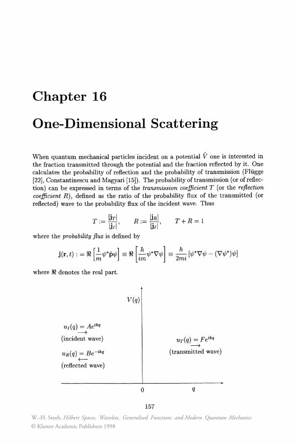
Chapter 16
One-Dimensional Scattering
When quantum mechanical particles incident on a potential V one is interested in the fraction transmitted through the potential and the fraction reflected by it. One calculates the probability of reflection and the probability of transmission (Fliigge [22], Constantinescu and Magyari [15]). The probability of transmission (or of reflection) can be expressed in terms of the transmission coefficient T (or the reflection coefficient R), defined as the ratio of the probability flux of the transmitted (or reflected) wave to the probability flux of the incident wave. Thus
where the probability flux is defined by
where ~ denotes the real part.
UI(q) = Aeikq
--+ (incident wave)
UR(q) = Be-ikq
+-(reflected wave)
V(q)
o
157
T+R=1
UT(q) = Feikq
--+ (transmitted wave)
q
W.-H. Steeb, Hilbert Spaces, Wavelets, Generalised Functions and Modern Quantum Mechanics© Kluwer Academic Publishers 1998
158 CHAPTER 16. ONE-DIMENSIONAL SCATTERING
In the following we consider the one-dimensional case. Then the probability flux takes the form
j(q,t):= 2~i ['Ij;*(q,t):q'lj;(q,t)- (:q'lj;*(q,t))'Ij;(q,t)] .
We consider first a free particle in one dimension. The Hamilton function is
p2 H(p,q) = 2m.
The quantization yields the Hamilton operator
• ;,,2 fJ2 H=----. 2maq2
Therefore the Schr6dinger equation is given by
The separation ansatz
gives
i;"a'lj; = H'Ij;. at
'Ij;(q, t) = e-iEt/liu(q)
;,,2 cPu ---=Eu.
2mdq2 The general solution to this linear differential equation with constant coefficients is
u(q) = Cleipq/Ii + C2e-ipq/1i
where C1 and C2 are the constants of integration. The energy takes the form
p2 E=-.
Since
we have
Then
2m
k = !!. ;"
By straightforward calculation we find that
It follows that
Therefore
From T + R = 1, it follows that
" - lik AA* JI- -m
" _ fikBB* JR--m
" _ fik FF* Jr-- "
m
FF* T= AA*
BB* R= AA*"
FF* + BB* = AA*.
159
To calculate the transmission coefficient and reflection coefficient we have to specify the potential. We consider two different potentials in the following.
Example 1. Particle incident on a Dirac delta potential, i.e.
V(q) = Vo8(q)
where Va > o. Thus the wave functions on the left and right hand sides of the delta function are given by
UR(q) = Feikq
respectively. Here L indicates left and R indicates right. Continuity of the wave function at q = 0 implies that
A+B=F.
The Dirac potential is discontinuous at q = O. Using the eigenvalue equation
fi2 d?-- 2m dq2 u(q) + Va8(q)u(q) = Eu(q)
160 CHAPTER 16. ONE-DIMENSIONAL SCATTERING
and integrating across q = 0
1i2 +< (d) +< +< - 2m j d d~ + j Vo8(q)u(q) dq = E j u(q) dq
-f -e -e
yields (€ -t 0)
. 2mVo -zk(F - A + B) + --;;;,rF = O.
We have used that
+<
limj V08(q)u(q) dq = Vou(O) <---.0
-<
. a-u . du du +< J? (I I) hm -dq=hm - --
<---'01. dq2 <---.0 dq q=< dq q=_<
and u(O) = F. From UL and UR we find
Consequently
The solution of
gives
and
dUL A 'k ikq B 'k -ikq -= ze - ze dq
dUR -F'k ikq - Z e . dq
lim j+< ~d ~ dq = Fik - Aik + Bik. <---.0 q
-<
A+B=F
ik(F - A + B) = 2m;0 F 1i
A = - mVoF F ikfi2 + , A* - mVoF* F*
- ikfi2 +
AA* = (- mVo 1) (mVo 1) FF*. ikfi2 + ik1i2 +
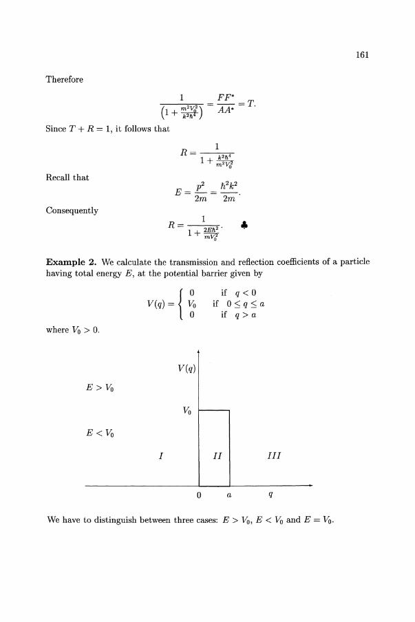
161
Therefore
1 FF*
(1 + ~:~l) = AA* = T.
Since T + R = 1, it follows that
Recall that
Consequently 1
R = 2E1i2 ' ..
1 + mY.' a
Example 2. We calculate the transmission and reflection coefficients of a particle having total energy E, at the potential barrier given by
where Va > O.
E>Va
V(q)
Va
if q < 0 if O~q~a
if q > a
I II III
o a q
We have to distinguish between three cases: E > Va, E < Va and E = Va·
162 CHAPTER 16. ONE-DIMENSIONAL SCATTERING
Case 1. E> 110 The general solution of the eigenvalue equation fI u( q) = Eu( q) in the three domains is given by
u(q) ~ { AeiPlq/1i + Be-iplq/Ii q<O Geip2q/1i + Fe-ip2Q/1i O<q<a CeiP1Q/1i + De-ipIQ/1i q>a
where
PI = J2mE, P2 = V2m(E - 110). Obviously, D = O. If a particle arrives at the barrier from the left, the terms with the coefficients A, Band C represent, respectively, the incident, the reflected, and the transmitted wave. The continuity conditions at q = 0 and at q = a for u and du/dq give
A+B
PI(A - B)
Eliminating G and F yields
B (pf - pD (1 - e2iP2ajli)
A - (PI + P2)2 - (PI - P2)2 e2ip2 a jli
C _ 4pIP2ei(P2-pJ)a/1i
A - (PI + P2)2 - (PI - P2)2e2ip2a/1i .
It follows that
T _I C I2 _ 4E(E - 110) - A - 1102 sin2 (rr) + 4E(E - 110)
and
I B 12 v,2 sin2 (l!1!!:.) R- _ _ 0 Ii
- A - 1102 sin2 (rr) + 4E(E - 110)
where R + T = 1. Reflection occurs with a non-vanishing probability. The barrier becomes completely transparent (R = 0, T = 1) if
. (P2 a ) sm h =0
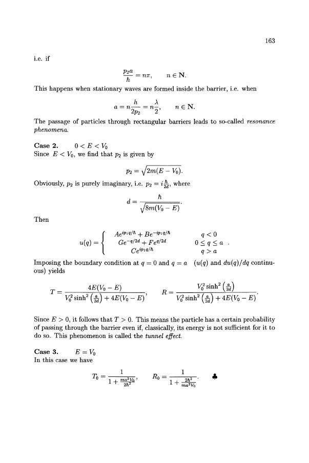
163
i.e. if
P2a h =mr, nE N.
This happens when stationary waves are formed inside the barrier, i.e. when
h A a = n- = n- n E N.
2P2 2'
The passage of particles through rectangular barriers leads to so-called resonance phenomena.
Case 2. 0 < E < Vo Since E < Vo, we find that P2 is given by
P2 = V2m(E - Vo). Obviously, P2 is purely imaginary, i.e. P2 = ifct, where
Then
u(q) ~ { AeiPlq/T1 + Be-iplQ/T1
Ge-q/ 2d + Feq/ 2d
CeiP1QjTl
q<O O::;q::;a
q>a
Imposing the boundary condition at q = 0 and q = a (u(q) and du(q)/dq continuous) yields
T = 4E(Vo - E) V02 sinh2 (fd) + 4E(Vo - E)'
V;2 sinh2 (..!!.) R= 0 2d .
V02 sinh2 (fd) + 4E(Vo - E)
Since E > 0, it follows that T > 0. This means the particle has a certain probability of passing through the barrier even if, classically, its energy is not sufficient for it to do so. This phenomenon is called the tunnel effect.
Case 3. E = Vo In this case we have
1 Flo = 1 2712 •
+ ma2Vo
164 CHAPTER 16. ONE-DIMENSIONAL SCATTERING
Exercises. (1) Consider the potential
Find the reflection and transmission coefficients for E > O. Find the eigenvalues for E<O.
(2) Let
V(q) = ac5(q - 1) + bc5(q + 1)
where a, b > O. Find the reflection and transmission coefficients for E > o.
Chapter 17
Solitons and Quantum Mechanics
Although nonlinear wave equations are very complex, some of them possess a unique property: they are exactly integrable. The techniques originated from a discovery, made by Gardner, Greene, Kruskal and Miura [23), who showed that the Kortewegde Vries equation may be exactly integrated by the inverse scattering problem technique. Here quantum mechanics plays the central role. This result was further developed by Lax, who formulated the Lax pair method (see Lamb [35), Ablowitz and Segur [1), Sagdeev et al [50)). Lax's ideas immediately found numerous generalizations. This started a period of discoveries of new partial differential equations which can be exactly integrated.
As an example we consider the integration of the Korteweg-de Vries equation. This partial differential equation is given by
The initial value problem was the first equation to be solved by the inverse scattering problem technique. To solve it we use the Lax pair method. First we introduce the Lax operator pair L and A for the Korteweg-de Vries equation. The linear operators L and A are partial differential operators. We set
L:= _D2 + u(x, t), a D:=-. ax
This operator acts on certain complex valued smooth functions 1/J{x, t), decreasing fairly rapidly as x -+ ±oo. We also assume that u possesses the same property.
Let us now consider an eigenvalue problem for the operator L, i.e.
L1/J = {-D2 + u{x, t))1/J = )"1/J .
165
W.-H. Steeb, Hilbert Spaces, Wavelets, Generalised Functions and Modern Quantum Mechanics© Kluwer Academic Publishers 1998
166 CHAPTER 17. SOLITONS AND QUANTUM MECHANICS
This equation is an eigenvalue equation with potential u(x, t). The variable t in this equation is considered as a parameter on which the potential u depends. Therefore both the eigenvalues A and eigenfunctions 'l/J depend on t.
Next we construct a unitary operator U(t) such that the product U-1(t)L(t)U(t) does not depend on the parameter t. This means that
U-1(t)L(t)U(t) = U-1(0)L(0)U(0) = L(O).
Applying the this operator equation on the function 'l/J(x, 0) == 'l/J(x, t = 0) gives
U-1(t)L(t)U(t)'l/J(x,0) = L(O)'l/J(x, 0) = A'l/J(X, 0).
If such an operator U does indeed exist, the eigenvalues A do not depend on t.
For the function u(x, t), which is the solution of the Korteweg-de Vries equation, the quantity t denotes the time. In the operators L, A, U, as well as in the eigenfunction 'l/J(x, t) the quantity t is just a parameter. Since the operator U is unitary we can write
U(t) = exp(iAt)
where A is a self-adjoint operator. Then the condition that U-l(t)L(t)U(t) does not depend on t leads to
~~ = i(AL - LA)(t) == irA, L](t)
where [, ] denotes the commutator. Since
'l/J(t) = U(t)'l/J(O) = eiAt'l/J{O)
we obtain the following linear partial differential equation for 'l/J(t)
: = -iA'l/J.
Let the potential u(x, t) in the eigenvalue equation be dependent on t as a parameter. Then all the Hamilton operators, comprising the one-parametric family L(t) for different t, are unitarily equivalent. Their eigenvalues A do not depend on t, while the eigenfunctions 'l/J vary with t.
Now we have to choose a specific form of A. From the definition of L we have simply
aL au at at'
We now set A = -iD. Then we obtain the partial differential equation au/at = au/ax. A nontrivial equation may be obtained by setting
A = i( -4D3 + 3(uD + Du)).
167
Then condition 8Lj8t = irA, L)(t) yields the Korteweg de Vries equation. In this case the eigenfunctions 'lj;(x, t) satisfy the partial differential equation
~~ = (-4D3 + 3(uD + Du))'IjJ.
Notice that Du'IjJ = D(u'IjJ) = (Du)'IjJ + u(D'IjJ).
If we consider the asymptotic forms as x -t ±oo, where u(x, t), according to the initial assumptions, vanishes fairly rapidly, then we obtain
x -t ±oo.
The integration of the linear partial differential equations gives
'IjJ(x, t) = e-4tD3 'IjJ(x, 0), x -t ±oo.
We can thus determine the dependence of 'IjJ(x, t) on t independently of L'IjJ = A'IjJ. It suffices to know 'IjJ(x,O). Not only the eigenvalues A can now be determined for initial conditions u(x, 0), but also the asymptotic forms of the eigenfunctions 'IjJ(x, t) as x -t ±oo.
We now determine from the eigenvalues A (independent of t) and the asymptotic forms of the eigenfunctions 'IjJ(x -t ±oo), the potential u(x, t) for an arbitrary value of the parameter t. This potential is a solution of the Korteweg de Vries equation.
We have shown that the problem of finding the solution of the Korteweg-de Vries equation can be reduced to reconstructing the Schrodinger equation potential from certain information on its eigenvalues and the asymptotic forms of its eigenfunctions. Let us define these data. First we consider the discrete spectrum. If u(x, 0) falls off fairly rapidly as x -t ±oo (one assumes that u(x, 0) E S(R)), then the operator L has only a finite number of nondegenerate eigenvalues An. We set
An = -~~. As x -t 00 the eigenfunctions behave as
X -t 00
where the en are the normalization constants. Substituting 'ljJn into the right-hand side of 'IjJ(x, t) = exp( -4tD3)'IjJ(X, 0) we obtain (since eaD3 efJx == ecxfJ3 efJX)
Now we consider the continuous spectrum of the operator L and put A = k2 . The asymptotic forms of a wave function as x -t ±oo may be written as
168 CHAPTER 17. SOLITONS AND QUANTUM MECHANICS
The following relations hold for the Schrodinger equation (for the operator L)
la±12 - Ib±12 = l.
Substituting 'l/J± into 'l/J(x, t) = e-4tD3 'l/J(x, 0), we find
Now let us write the problem of scattering by a potential in its standard form. This means
b+(k, O) = r(k, 0), a- (k, 0) = d(k, 0),
where we have introduced complex transmission and reflection amplitudes, rand d
Irl2 + Idl2 = l.
To keep the amplitude of the incident wave equal to unity for any t, we must set
(k t) = b+ (k, t) = 8ik3t (k 0) r, a+(k, t) e r, .
Similarly, it follows
We define
N 1 J . B(z) := ~ C~e-Nnz + - dkr(k)e<kz n=l 27r R
where N is the number of eigenvalues in the discrete spectrum. We use this function when reconstructing the potential from scattering data, using the Gelfand-LevitanMarehenko integral equation
00
K(x, y) + B(x + y) + J dzB(y + z)K(x, z) = 0 x
for an unknown function of two variable K(x, y). This equation is linear. The potential u(x) may be determined from its solution as follows
d u(x) = -2 dxK(x, x).
Taking into account the fact that en and r(k) are time-dependent, we should treat B as a function of z and t. We must substitute expressions for Cn(t) and r(k, t) into B(z) to find
B(z, t) = t C~(k, 0) exp(N!t - Nnz) + 21 J dk r(k, 0)ei (8k 3t-kz). n~ 7rR
169
We thus have
d u(x, t) = -2 dx K(x, Xj t).
This solves the problem of integrating the Korteweg-de Vries equation.
A certain special class of initial conditions u(x, t = 0) = u(x,O) exists for which an exact solution can be written down explicitly. These are the so-called N -soliton solutions. Solving the Korteweg de Vries equation begins with specifying the initial condition u(x, 0). We set
u(X,O) = -2sech2x
where sechx == 1/ cosh x. The eigenvalue problem for the potential u(x,O) = -2sech2x can be solved exactly. There is only one solution in the discrete spectrum Nl = 1, C1(0) = v'2. However, there is no reflected wave in its continuous spectrum, that is, b(k,O) = 0 for any k. A particle with an arbitrary energy A = k2
cannot discover the presence of the potential. Substitution of formulas Nl = 1, C1(0) = v'2 and b(k, 0) = 0 into the expression for B(z, t) yields
B(z, t) = 2eSt- z
whence the Gelfand-Levitan Marchenko integral equation takes the form
00
K(x, Yj t) + 2eSt- x - y + 2eSt- y J dzK(x, Zj t)e-Z = o. x
This equation can be solved by a separation of variables. Assuming that
K(x, Yj t) = Ko(xj t)e-Y
we obtain
2 K(x,xjt) = - ( ) 1 +exp 2x - 8t
Hence the solution of u(x, t) is
u(x, t) = -2sech2 (x - 4t).
This is a travelling soliton. If b(k, t) = 0, i.e. the potential u(x, 0) is reflection-free, then solving the Gelfand-Levitan-Marchenko integral equation yields an N-soliton solution. For the calculation of the N-soliton solutions we refer to the literature (Sagdeev et al [50]).
170 CHAPTER 17. SOLITONS AND QUANTUM MECHANICS
Exercises. (1) Show that the sine-Gordon equation
f)2u 8tax = sinu
can be obtained from the eigenvalue equation
fhfJI. 1 au ax + z)..'r/h = -"2 ax'l/J2
a'l/J2 _ i>''l/J2 = ! aU'l/Jl ax 2ax
and the time-evolution equations
a'l/Jl i . at = 4>. ('l/Jl cos U + 'l/J2 sm u)
a'l/J2 i . at = 4>. ('l/Jl sm u -'l/J2 cos u) .
(2) Let x = (Xl, X2, ... ), a == a/aXl and
Xl
a-lf(x) = ! f(S,X2, ... )ds.
Consider a system of linear equations for an eigenfunction and an evolution equation
Show that
and
Let
L(x, a)'l/J(x, >.) = >''l/J(x, >.)
a'l/J ~ = Bn(x, a)'l/J(x, >.). uXn
aL ~=[Bn,Ll uXn
L = a + U2(X)a-l + U3(X)a-2 + .... Define Bn(x, a) as the differential part of (L(x, a))n. Show that
Chapter 18
Perturbation Theory
In this chapter we show that the Rayleigh-Schrodinger perturbation theory is a special case of a solution of an autonomous system of differential equations. Furthermore, we discuss perturbation theory for an anharmonic oscillator. Let
H, = Ho + t:1I be a Hamilton operator with discrete spectrum for t: ;::: o. Assume further that the eigenvalues are not degenerate. Eigenfunctions are assumed to be real orthonormal. Furthermore the eigenvalues and eigenfunctions of Ho are known.
Degeneracies of eigenvalues are in general related to symmetries of the Hamilton operator H. If the Hamilton operator H admits discrete symmetries the Hilbert space can be decomposed into invariant subspaces with respect to H (see chapter 11). These invariant subspaces are again Hilbert spaces and the perturbation expansion can be performed in these subspaces.
Our goal is to calculate the eigenvalues En as a function of Eo We define
Iun(t:)) : eigenfunctions of H,
where we assume that the eigenfunctions form an orthonormal basis in the underlying Hilbert space. Furthermore we define
(m f. n)
171
W.-H. Steeb, Hilbert Spaces, Wavelets, Generalised Functions and Modern Quantum Mechanics© Kluwer Academic Publishers 1998
172 CHAPTER 18. PERTURBATION THEORY
In the following derivation we use
L IUn(E)) (un(E)1 = I completeness relation. nEI
From
it follows that
IT dlun(E)) V"I ()) V" dIUn(E)) _ dEn(E) I ()) E ( )dlun(E)) flO dE + un E + E dE - dE Un E + n E dE .
Taking the scalar product with (un(E)1 we obtain
where we have used
Since
we find
dEn(E) _ () ~-PnE.
Taking the scalar product with (um(E)1 we obtain (m =1= n),
(um(E)I(Ho + EV) dlu~;E)) + (um(E)IVlun(E)) = En(E)(Um(E)ldlu~;E)) where we have used that
Since
and
it follows that
173
From
we find
Therefore
d(um(€) I Vmn (€) = [Em(€) - En(€)] d€ Iun(€)).
Let us now calculate dPn/d€. We obtain
Using the completeness relation it follows that
Since
we find
Inserting the expression for d(um(€)I/d€lu n(€)) given above yields
Consequently,
where
Let us now calculate dVmn/d€ where m =f. n. We obtain
174 CHAPTER 18. PERTURBATION THEORY
Using the completeness relation gives
or
Consequently,
or
dVmn '" [ (1 1)] Vmn (p ) -d- = L...J Vrnlvtn E _ E + E _ E + E _ E n - Pm . f l#(m,n} m l n l m n
To summarize. We find the following autonomous system of first order ordinary differential equations
dEn -=Pn df
This system of differential equations must be solved together with the initial conditions
This means that the eigenvalues and eigenfunctions of Ho must be known, i.e., En(f = 0), Un(f = 0).
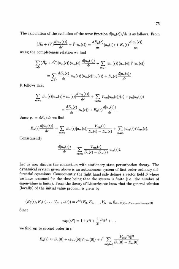
175
The calculation of the evolution of the wave function dlun(E)/dE is as follows. From
(fIo + EV) dlu~~E) + VIUn(E) = dE;?) IUn(E) + En (E) dlu~~E) using the completeness relation we find
L (fIo + EV) IUm(E)(Um(E)1 dlu~(E) + L IUm(E)(Um(E)!Vlun(E) mEl E mEl
It follows that
L Em(E)IUm(E)(Um(E)ldlu~~E) + L VmnIUm(E)(E) + PnIUn(E) m#n m#n
_ dEn(E) I () E ( )d1un(E) - dE UnE+n E dE'
Since Pn = dEn/dE we find
En(E) dlu~~E) = En Em(E)IUm(E) En(~m-=(~m(E) + En IUm(E))Vmn(E).
Consequently
Let us now discuss the connection with stationary state perturbation theory. The dynamical system given above is an autonomous system of first order ordinary differential equations. Consequently the right hand side defines a vector field S where we have assumed for the time being that the system is finite (i.e. the number of eigenvalues is finite). From the theory of Lie series we know that the general solution (locally) of the initial value problem is given by
Since
122 exp( ES) = 1 + ES + IE S + ... 2.
we find up to second order in E
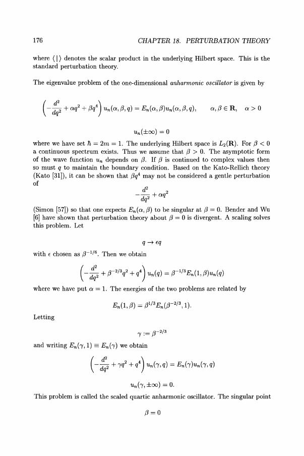
176 CHAPTER 18. PERTURBATION THEORY
where (I) denotes the scalar product in the underlying Hilbert space. This is the standard perturbation theory.
The eigenvalue problem of the one-dimensional anharmonic oscillator is given by
a,/3 E R, a> 0
Un(±OO) = 0
where we have set Ii = 2m = 1. The underlying Hilbert space is L2(R). For /3 < 0 a continuous spectrum exists. Thus we assume that /3 > o. The asymptotic form of the wave function Un depends on /3. If /3 is continued to complex values then so must q to maintain the boundary condition. Based on the Kato-Rellich theory (Kato [31]), it can be shown that /3q4 may not be considered a gentle perturbation of
cP 2 --+aq dq2
(Simon [57]) so that one expects En(a, /3) to be singular at /3 = o. Bender and Wu [6] have shown that perturbation theory about /3 = 0 is divergent. A scaling solves this problem. Let
q -+ fq
with f chosen as /3-1/6. Then we obtain
( - :;2 + /3-2/3q2 + q4) un(q) = /3-1/3 En(l, /3)un(q)
where we have put a = 1. The energies of the two problems are related by
Letting
, := /3-2/3
and writing En(r, 1) == En(,) we obtain
( -!2 + ,q2 + q4) un(r, q) = En (r)un(r, q)
un(r, ±oo) = O.
This problem is called the scaled quartic anharmonic oscillator. The singular point
/3=0
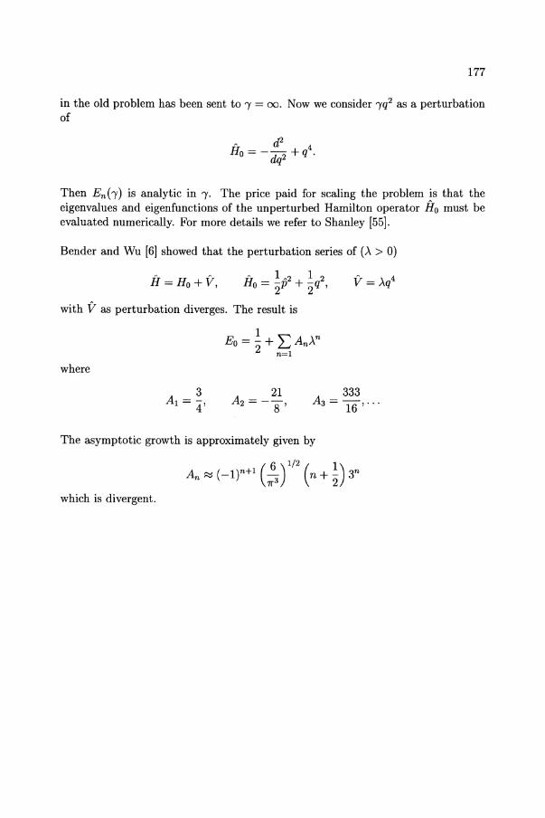
177
in the old problem has been sent to "( = 00. Now we consider "(q2 as a perturbation of
A d2 4 Ho = - dq2 + q .
Then En("() is analytic in "f. The price paid for scaling the problem is that the eigenvalues and eigenfunctions of the unperturbed Hamilton operator fIo must be evaluated numerically. For more details we refer to Shanley [55].
Bender and Wu [6] showed that the perturbation series of (,\ > 0)
with V as perturbation diverges. The result is
where
333 A3 = 16'···
The asymptotic growth is approximately given by
which is divergent.
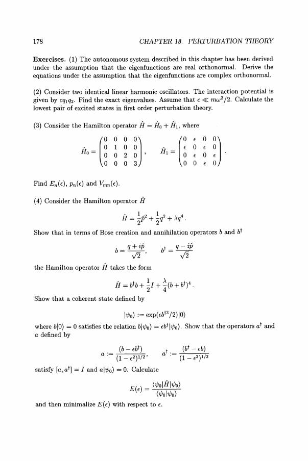
178 CHAPTER 18. PERTURBATION THEORY
Exercises. (1) The autonomous system described in this chapter has been derived under the assumption that the eigenfunctions are real orthonormal. Derive the equations under the assumption that the eigenfunctions are complex orthonormal.
(2) Consider two identical linear harmonic oscillators. The interaction potential is given by cqlQ2. Find the exact eigenvalues. Assume that c« mw2/2. Calculate the lowest pair of excited states in first order perturbation theory.
(3) Consider the Hamilton operator H = Ho + Hl , where
(
0 0 A 0 1
Ho = 0 0
o 0 ~ ~), o 3
H = (~ ~ ~ 1 0 E 0
o 0 E
(4) Consider the Hamilton operator H
H = ~p2 + ~q2 + >.q4 . 2 2
Show that in terms of Bose creation and annihilation operators band bt
b = q + ip y'2'
the Hamilton operator H takes the form
Show that a coherent state defined by
Iwo) := exp( Ebt2 /2) 10)
where blO) = 0 satisfies the relation blWo) = Ebt IWo). Show that the operators at and a defined by
satisfy [a, at] = I and alwo) = O. Calculate
E(E) = (WoIHIWo) (WoIWo)
and then minimalize E(E) with respect to E.
Chapter 19
Helium Atom
The Hamilton operator if of an atom with Z-electrons and Z-protons (in the nucleus) is given by (Schiff [51])
H= --E~i - -~N- -E - E-:------:-, ",2 Z ",2 e2 Z (z Z 1 )
2me i=l 2mN 47r£0 i=l ITi - TNI #i ITi - Tjl
where me is the mass of the electron and mN the mass of the nucleus. The first term describes the kinetic contributions from the electrons and the second the kinetic contribution from the nucleus. The third term gives the interaction of the nucleus with the electrons (attractive force) and the fourth the interaction of the electrons (repulsive force).
For the Helium atom we have Z = 2. Since
me < 0.545 . 10-3 mN -
we can assume that the nucleus is at rest. We put TN = 0, i.e., the nucleus is at the origin. Thus the Hamilton operator takes the form
where
with TI = (Xl, Yb Zl) and f2 = (X2, Y2, Z2). The underlying Hilbert space is L2(R6).
The eigenvalue problem cannot be solved exactly. We would like to find the ground state in an approximative manner with the help of a variational principle.
179
W.-H. Steeb, Hilbert Spaces, Wavelets, Generalised Functions and Modern Quantum Mechanics© Kluwer Academic Publishers 1998
180 CHAPTER 19. HELIUM ATOM
Variational Principle. Let H be a Hamilton operator with discrete spectrum. Assume that the spectrum is bounded from below. Denote by Eo the lowest eigenvalue. Let u E 11. where 11. is the underlying Hilbert space with u =I- o. Then
(u,Hu) Eo 5:. -'-:-----:--'-(u, u) .
If u is normalized, then Eo 5:. (u, Hu).
Proof. Let {un: n E I} be the eigenfunctions of H. Assume that {un n E I} forms an orthonormal basis in the underlying Hilbert space 11.. Since
we obtain
(u, HU) = L L C';,. en En (um, un) = L L c';,.cnEnomn = L c';,.emEm = L leml2 Em· mEl nEI mEl nEI mEl mEl
Since
mEl mEl we obtain
(u, HU) ;::: Eo L leml2 = Eo(u, U). mEl
Consequently, the inequality follows. •
For the Helium atom we make the product ansatz
where
of the type of ground state of H -atom.
This means the wave function ulJ E L 2 (R6) has only a radial part. Here J.t is a real parameter. The parameter J.t is determined so that
becomes a minimum.
(u/-I(rI, r2), HU/-I(rl, r2))
(U/-I(rl,r2),U/-I(rl,r2))
The calculation of the expectation values with the wave function (5) yields
(rll) = (ril) = / u!(r)r- l sin ()d()dcpdr = f.L R3
/00/00/1 e-2/-1(rl +r2) 5f.L
(rI2l) = 8f.L3 r~ drlr~ dr2 dx = S· o 0 -1 yr? + 2rlr2x + r~
We made use of the fact that in spherical coordinates we can write
Irl - r21 = Jr? - 2rlr2 cos () + r~ and x = cos (). Therefore dx = - sin ()d().
Consequently,
Minimalizing with respect to f.L yields
27 e2 m 27 m 1 f.L=f.Lo = ---2 = ---
16 411"€0 1i 16 me ao
where
Consequently
where 1
Uf := 137.0381
The experimental data are:
He He+ He
m'-.- me+mN
Sommerfeld fine structure constant.
He+ + e He++ + e He++ + 2e-
-24.5878 eV -54.4144 eV -79.0022 eV
181
182 CHAPTER 19. HELIUM ATOM
The spin of the electrons of the helium atom was not included in our calculation. Let the operator 0"12 be defined by
0"12u(r1, r2) := U(r2' rd
i.e., it interchanges the spatial coordinates of the two electrons. The operator 0"12 is called a permutation operator. The Hamilton operator if of the helium atom is unchanged when the coordinates of the two electrons are interchanged. Consequently, u(r2' r1) must be a solution of the eigenvalue equation if u(r1' r2) is a solution. If u(r1' r2) corresponds to a non-degenerate eigenvalue, u(r1' r2) and u(r2' r1) can only differ by a mUltiplicative factor .\,
u(r2' r1) = 0"12u(r1, r2) = .\u(r1' r2) .
Applying the permutation operator 0"12 twice, we obtain u(rl' r2) again, i.e.,
0"~2u(r1,r2) = .\0"12u(r1,r2) = .\2u(r1,r2) = u(r1,r2).
Consequently, .\2 = 1 or .\ = ±l.
Wave functions with
u(rl, r2) = u(r2' rd
are called space symmetric and denoted by u+(r1, r2) (also called para states). Wave functions with
u(r1' r2) = -u(r2, r1)
are called space antisymmetric and denoted by u_(rl,r2) (also called ortho states).
The full eigenfunctions of the system must be tensor products of the spatial eigenfunctions u(rl, r2) (satisfying the eigenvalue equation) times spin wave function X(I,2) for the two electron system
it(rl, 81, r2, S2) = u(rl, r2)x(I, 2) == u(rl, r2) Q9 X(I, 2) .
where Q9 denotes the tensor product. The Pauli exclusion principle requires that the total wave function
of a system of N electrons must be antisymmetric. In other words it must change sign if all coordinates (spatial as well as spin) of two electrons are interchanged. In our example for the helium atom the test wave function is a symmetric spatial wave function (para state). Consequently, the spin state must be antisymmetric.
Chapter 20
Potential Scattering
The typical two-particle scattering experiment is as follows (Prugovecki [47], Fliigge [22], Gasiorowicz [24]). A beam of particles 81 impinges on a target consisting of particles 8 2 . Assuming that the particles in the beam do not interact with one another, and that each particle 8 1 in the beam interacts with only one particle 82
in the target, the experiment can be viewed as consisting of a large ensemble of independent scattering experiments of a two-particle system 8 = {81, 82}. The two mentioned conditions can be satisfied by taking a "weak" beam of particles (i.e., a beam with few particles per unit volume), and taking for the target a slab of material which is sufficiently thin to eliminate the possibility of a particle 8 1
scattering from more than one particle in the target. The above experimental setup is suited to determine the percentage of the particles in the beam which can be found in a given volume of space, occupied by a detector, after they have been scattered by the target. In any scattering experiment the detector is placed sufficiently far from the target so that it does not interfere with the scattering process. Hence, the experiment obviously provides information about the probability that a particle of the beam, coming towards the target from the direction
Wo = (¢o, (}o),
will be scattered within the solid angle dw around the direction
w = (¢, (}), o ::; (} ::; 7['.
If N denotes the number of two-particle scatterings per unit time at the energy of relative motion E, then the number of particles scattered within the solid angle dw can be written in the form N1T(E,wo,w)dw, since it is obviously proportional to N as long as the two earlier mentioned conditions on beam and target are satisfied. It can be expected that 1T(E,wo,w) is dependent on the energies E and E' for the relative motion of the particle of, the system 8 = {81> 82} before and after collision. However, since energy is conserved,· we must have E = E', . so' that the dependence on E' does not have to be displayed.
183 W.-H. Steeb, Hilbert Spaces, Wavelets, Generalised Functions and Modern Quantum Mechanics© Kluwer Academic Publishers 1998
184 CHAPTER 20. POTENTIAL SCATTERING
One orientates the frame of reference so that <Po = (}o = O. Let Jo be the incident flux, i.e., the number of incident particles per unit time and unit beam cross section. We call the quantities
N a(E,w):= Jo 7r(E,wo,w), aCE) := J a(E,w)dw
Os
the differential cross section and the total cross section, respectively. The notation da/dw instead of a(E,w) is often used.
In non-relativistic quantum mechanics, the scattering of particles of mass m, momentum kli and energy E by a potential VCr) is determined by the asymptotic behaviour of the solution 1/J~(r), corresponding to out-going scattered waves, of the eigenvalue equation
where
and
A 2m A
U(r) := /i2V(r)
k2 _ 2mE - li2
A solution of the eigenvalue equation in the absence of a potential V is the plane wave solution exp(ik . r) associated with the eigennumber
.:\(k) =~. 2m
Notice that exp(ik . r) fj. L2 (R3). If the potential has a finite range, i.e., if VCr) is appreciably different from zero only for Irl ::; ro the problem of solving the eigenvalue equation with the appropriate boundary conditions is equivalent to that of solving the Fredholm-type integral equation
1/J~(r) = <Pk(r) - ~ J exp~iklr I r'D U(r')1/Jt(r')dr' 47T r - r'
where
<Pk(r) = exp(ik· r) .
As mentioned above <Pk satisfies the homogeneous equation
(~+ k2)¢k(r) = o. For the derivation of integral equation we use the fact that the fundamental solution of the equation (see chapter 4 on generalized functions)
is given by
Let r := Irl. At large distances from the scattering centre (r » ro) we have
r »ro
where r = (r, 0, c/J) in spherical coordinates having k as polar axis, and
k' = k~. r
185
A(E, 0, c/J) is called the scattering amplitude. The differential scattering cross-section is then
da(E, 0, c/J) = IA(E, 0, c/JWdO, dO = sin OdOdc/J.
Integrating this expression over all directions, we obtain the total scattering crosssection
a(E) = f da(~;, c/J) dD.
The scattering amplitude obtained by using the zero-order approximation
1jJ~(r) = c/Jk(r)
for the solution of the Fredholm-type integral equation is called the Born amplitude. To find the condition of the validity of the Born approximation is left as an exericse. The Born amplitude can be written in the form
Let
fiq := fi(k - k')
be the momentum transferred on scattering. Then we can write
The ratio
186 CHAPTER 20. POTENTIAL SCATTERING
A(B)(q) F(q) = A(B)(O)
is called the form factor and it characterizes the interference between waves scattered in different volume elements of the scattering field.
The mutual elastic scattering of two particles with masses ml and m2 and a potential energy of interaction V(r2 - rl) can be expressed in terms of the motion of particle 1 relative to particle 2, which is formally identical with that of a single particle of reduced mass
mlm2 m := --"--=--
ml +m2
moving in a potential V(r) referred to a fixed origin. Thus, in the centre of mass system of the two particles, the direction of motion after scattering of particle 1, ((),4», coincides with that of the hypothetical single particle and is related to the directions of motion after scattering, (()l, 4>1) and (()2, 4>2), of particles 1 and 2 in the laboratory system (in which the second particle was at rest before the scattering occurred) by the relations
sin () tan ()l = ()'
'Y + cos
1 ()2 = -(71" - ()),
2
Next we study the method of partial waves. For a central potential we have
V(r) = V(r).
The direction of the momentum of the incident particle constitutes an axis of symmetry of the problem. Choosing the polar axis in this direction, the solution of the eigenvalue equation will be independent of 4>. Consequently
~ R1k(r) 'lj;t(r,()) = ~al-'-.li(Cos()) 1=0 r
where
al := il(2l + l)eiOI (k)
and .Ii denotes the Legendre polynomials (see chapter 1) with l = 0,1,2,. .. . The functions Rl,k (r) are the solutions of the radial equation
d2R1,k 2m (E _ (V() l(l + 1)h2)) R = 0
dr2 + h2 r + 2mr2 I,k.
The boundary condition at r = 0 is given by R1,k(r = 0) = o. Furthermore the functions Rt,k have the following asymptotic behaviour for large r
187
RI,k(r) ~ ~ (kr - l; -81(k))
for potentials which vanish at infinity faster than r-1 and are less singular at the origin than r-2. This asymptotic behaviour of Rl,k(r) corresponds to the normalization
00 ! RI,k(r)R1,k,(r)dr = 2~28(k - k') o
where 8 is the delta function. For large r, we write the outgoing parts of the partial waves of 'l/Jt in the form
where ¢tk(r, 0) is the outgoing part of the l-state wave function for the limiting case of a zero 'scattering potential. The effect of the non-zero potential then appears in the phase shift factor. Thus the scattering due to a central potential can be represented as a unitary transformation of free outgoing partial waves by a scattering operator, which, in the angular momentum representation, takes the simple form of a diagonal "scattering matrix" whose elements are
Sll' = exp[2i81(k)]811'
where 811' denotes the Kronecker delta. The various functions associated with elastic scattering are thus the phase-shifts 81(k), the eigenvalues of the scattering matrix
SI(k) = exp[2i81(k)]
known as the S-functions for each value of the orbital angular momentum l of the partial waves, the partial wave amplitudes
AI(E) = 2~k (SI(k) - 1) = ~eiOI(k) sin81(k)
the scattering amplitude
00
A(E,O) = I)2l + 1)A1(E)11(cos(}) 1=0
the differential cross section for elastic scattering
da(E,O) = IA(E,OWdO
the total cross section for elastic scattering
a(E) = I: a(!)(E) = !: I:(2l + 1) sin2 81(k) = ~ ~A(E, 0) 1=0 1=0
where ~ denotes the imaginary part.
188 CHAPTER 20. POTENTIAL SCATTERING
Exercises. (1) Find the differential cross section in the Born approximation for the potential
, A (r) V(r) = - exp --r ro
where A is a positive constant.
(2) Consider the scattering of a particle by a simple cubic lattice with lattice constant d. The interaction with the lattice points ri is described by the potential
, -27ran2
V(r) = L o(r - ri). m i
Treat the scattering in Born approximation. Show that the condition for nonvanishing scattering is that the Bragg law is satisfied.
(3) Formal scattering theory introduces the M{lIller operator n+ which carries an asymptotic state (an eigenstate of Ho) into the actual interacting state an eigenstate of the full Hamilton operator H = Ho + V. The MliSller operator satisfies the intertwining relation Hn+ = n+Ho. For potential scattering the domain of n+ is the full Hilbert space, but if the potential can support bound states, the range of n+ is the subspace spanned by the scattering states of H. Thus n+ is not unitary but only an isometry and satisfies n~n+ = I, n+n~ = R, where R is the projection on the subspace of scattering states. Show that (n+Hon:;:1 - Ho)R = V R, where we use that n~ acts like n:;:1 on the scattering states. The generator A+ of the MliSller operator is defined as n+ =: exp(A+). The linear operator adB is defined as (adB)X := [B, Xl for an arbitrary linear operator X. Show that exp(A)X exp( -A) == exp(adA)X. Show that we can write
((exp(adA+) - I)Ho)R = VR
This equation can be viewed as operator equation for A+ and therefore n+. Show that the equation can be rewritten as (¢(A+)[A+, Ho])R = V R, where the linear operator ¢(A+) = (exp(adA+) - 1)/(adA+)
1 1 ¢(A+)X = X + ,[A+, Xl + ,[A+, [A+, Xll + ....
2. 3.
To solve this equation for A+ it is necessary to invert the operator adHo. The inverse is uniquely determined when its diagonal part (in the basis of Ho) is required to vanish. Show that
00
(adHo)-1 X := ilim f exp( -lOt) exp( -Hot)(X - d(X)) exp(iHot)dt. <-+0
o Show that an expansion for A+ in powers of the interaction can now be obtained by equating terms of equal order.
Chapter 21
Berry Phase
The adiabatic theorem of quantum mechanics states that a quantum mechanical system prepared in an eigenstate of its Hamilton operator will remain in an instantaneous eigenstate, as the Hamilton operator is varied, provided that the variation is carried out slowly enough (Schiff [51], Messiah [41]). If the motion is cyclic, then the system will return to its original eigenstate multiplied by a dynamical phase factor. Berry [8], [9) showed that this theorem is incomplete. In addition to the dynamical phase, the system will also acquire a geometrical phase. This phase is non-integrable and depends on the path transversed in parameter space.
In this chapter we give a review of Berry's analysis (Berry [8), [9], Vinet [66]). First we study the adiabatic approximation. Let H(C(t)) be a Hamilton operator depending on the parameter
C(t) = (C1 (t),C2(t), ... ,Cm (t))
which vary slowly with time t. The state It) evolves according to the Schrodinger equation
a A
iii at It) = H(C(t))lt).
At any instant the instantaneous eigenstates satisfy
H(C)ln, C) = En(C)ln, C).
We assume that the states In, C) are normalized, i.e.
(n, Cin, C) = 1.
We consider first the case where the state In, C) is non-degenerate. The adiabatic theorem states that a system prepared at t = 0 in one of these states, e.g. In, C(O)), will be in the state In, C(t)) at t. It follows that an approximate solution to the Schrodinger equation is given by
189
W.-H. Steeb, Hilbert Spaces, Wavelets, Generalised Functions and Modern Quantum Mechanics© Kluwer Academic Publishers 1998
190 CHAPTER 21. BERRY PHASE
It) = exp (* I dtIEn(C(tl))) ei'Yn(t) In, C(t».
Since physical states correspond to rays in a Hilbert space H, we have introduced an extra phase in addition to the standard dynamical factor. Substituting this state into the Schrodinger equation, we find that I obey the equation
:tln(t) = i(n,CI (!In, C)) = iA(C)· !C
where
A(C) := (n, ClV'ln, C)
and V' denotes the gradient, i.e.
V' := (a~l' a~2 ' ... , a~m) T The quantity In is real since In, C) is normalized. We see that A is a vector potential on parameter space. There is a gauge freedom. If the phases of the instantaneous states are changed to
In, C) ---+ eiO(C) In, C).
A( C) is transformed into
A(C) ---+ A(C) + iV'B(C).
The phase ei'Yn is usually omitted on the basis that it can be absorbed into the instantaneous eigenstates In, C) (see for example Schiff [51]). It is argued that a smooth choice of gauge for the In, C) can be made so that A(C) = o. Berry's main contribution (Berry [8]) was to observe that this cannot always be done globally and that there are systems for which we cannot dispense with the vector potential A(C).
Let us consider the case where the time evolution is periodic so that the parameters return to their original values C(O) after some large time T, i.e.
C(T) = C(O).
The accumulated phase over the cycle C referred to as Berry's phase, is given by
T T
I = Jdtd,n(t) = JdtdC(t) .A(C(t»=i f dC·A(C). n dt dt
o 0 C={JS
Let m = 3. Converting the above line integral into a surface integral through Stokes theorem, we arrive at
with
In = i J dS· F s
F(C) = V' x A(C).
191
This is an invariant quantity which is unaffected by choices of phases of the wave functions. There are examples where Berry's phase does not vanish and where nontrivial holonomy occurs. We call A the Berry connection and F the associated curvature.
In the Born-Oppenheimer approximation, rather then treating the parameters C adiabatically, one quantizes them. Suppose for illustration that the kinetic energy for the slow variables is of the form P2/2M, the full Hamilton operator K is then given by
, p2 , K = 2M + H(C(t)).
One now seeks eigenfunctions of K in the form
w(C) = 1jJ(C) In, C).
By projecting the complete eigenvalue equation
K'1l = E'1l
on In, C) and neglecting the off-diagonal elements, one obtains for 1jJ(C) the following equation where In, C) is non-degenerate
where
1 V(C) = En(C) + 2M L (V'n, CJn', C) (n', CJV'n, C).
n'#-n The effective Born-Oppenheimer potential consists of the fast energy eigenvalue while the kinetic term is analogous to that of a particle in a magnetic field. One assumes that the phases of the states In, C) can be chosen so that these wavefunctions are real in which case A = O. From Berry's work we know that it might be impossible to remove the phase in this fashion.
Remark. The Born-Oppenheimer approximation implies gauge potentials of electric and magnetic type in the Hamilton operator governing the slow part of the system. Berry and Lim [10] demonstrated that the eleG:trkgaugepotential is repulsive in the space of slow parameters at which energies of the fast system are degenerate.
192 CHAPTER 21. BERRY PHASE
So far, we have only discussed situations where the state In, C) is non-degenerate. Suppose now that there are degeneracies and let the index a label the degenerate instantaneous states of a certain eigensubspace of H(C) : In, C, a), a = 1,2, .... The results in this case are similar to the ones presented above except that the connection is now a matrix
Aab = (n,C,aIVln,C,b).
The phase freedom is replaced by unitary transformations
In, C, a) -+ Ualaln, C, a')
under which A transforms as
Aab -+ U;')Aa1bIUb1b + U;')VUalb
where we used sum convention. The curvature acquires an additional term beyond the curl
Fab = V x Aab + (A x A)ab
Let us now examine a few examples where this gauge structure will appear. We calculate the Berry phase
In = i f dC· (nIVn) c=as
in a simple case. Let us first obtain following Berry [8], an expression for In that is more tractable than this expression. A direct evaluation of the above line integral requires locally single-valued In) and can be awkward. It is easier to use the surface integral
where
In = f dS· iF s
iF = -CSV x (nIVn).
Inserting a complete set of states, one has
iF = -CS(Vnl x IVn) = -CS L (Vnlm) x (mIVn). m#-n
193
The exclusion in the summation is justified by the fact that (nlV'n) is imaginary. From
H(C)ln) = En(C)ln)
one obtains for the off-diagonal matrix elements
1 A
(mlV'n) = En _ Em (mlV' Hln)
Substituting this into iF yields
iF = _~ L (nlV' Him) x (mlV' Hln) . m#-n (En - Em)2
Finally let us discuss Berry's paradigm example. Consider the Hamilton operator
All 1 1 H:=-u·C=-Xa +-Ya +-Za
2 2 "2 Y 2 z
with
C = (X,Y,Z)
and
as the Pauli matrices (see chapter 9). Since
the eigenvalues of H are given by
c:= IC!.
Therefore the quantum numbers n only take two values. Obviously
A 1 V'H = 2u.
We rotate the axes so that the Z-axis points along C. We find
A 1 H = 2Caz.
The eigenvectors of H are given by I t) and I.j..). We have (see chapter 8)
azl t) = It), azl .j..) = -I .j..)
194 CHAPTER 21, BERRY PHASE
O'x\ t) = \.J..), O'x\.J..} = \ t}
O'y\ t} = i\.J..), O'y\.J..) = -i\ t},
We study the adiabatic evolution of the state \ t), With respect to the rotated axes, we find
'F __ ~ (t \O'x\ .J..)(.J.. \O'y\ t) ___ 1_ z z - 2C2 - 2C2 '
Returning to unrotated axes, we obtain
'F C z = - 2C3'
Consequently, the Berry phase is given by
It is in general non-zero and equal to the flux through C = as of the magnetic field of a monopole with strength -1/2!.
Chapter 22
Measurement and Quantum States
22.1 Introduction
The interpretation of measurements in quantum mechanics is still under discussion (Healey [28], Bell [5], Redhead [48]). Besides the Copenhagen interpretation we have the many-worlds interpretations (Everett interpretations), the modal interpretations, the de coherence interpretations, the interpretations in terms of (nonlocal) hidden variables, the quantum logical interpretations.
A satisfactory interpretation of quantum mechanics would involve several things. It would provide a way of understanding the central notions of the theory which permits a clear and exact statement of its key prinicples. It would include a demonstration that, with this understanding, quantum mechanics is a consistent, empirically adequate, and explanatorily powerful theory. And it would give a convincing and natural resolution of the" paradoxes". A satisfactory interpretation of quantum mechanics should make it clear what the world would be like if quantum mechanics were true. But this further constraint would not be neutral between different attempted interpretations. There are those, particularly in the Copenhagen tradition, who would reject this further constraint on the grounds that, in their view, quantum mechanics should not be taken to describe (microscopic) reality, but only our intersubjectively communicable experimental observations of it. It would therefore be inappropriate to criticize a proposed interpretation solely on the grounds that it does not meet this last constraint. But this constraint will certainly appeal to philosophical realists, and for them at least it should count in favor of an interpretation if it meets this constraint.
It is well known that the conceptual foundations of quantum mechanics have been plagued by a number of "paradoxes," or conceptual puzzles, which have attracted a host of mutually incompatible attempted resolutions - such as that presented by Schrodinger [53], popularly known as the paradox of Schrodinger's cat, and the EPR "paradox," named after the last initials of its authors, Einstein, Podolsky, and Rosen [19].
195
W.-H. Steeb, Hilbert Spaces, Wavelets, Generalised Functions and Modern Quantum Mechanics© Kluwer Academic Publishers 1998
196 CHAPTER 22. MEASUREMENT AND QUANTUM STATES
22.2 Measurement Problem
Consider a spin - ~ particle initially described by a superposition of eigenstates of Sz, the z component of spin:
where
(t= SzlSz =t) = I,
and
(<I>I<I» = 1 .
Thus
ICll2 + IC212 = 1.
Let IR =t) and IR =.t) denote the up and down pointer-reading eigenstates of an Sz-measuring apparatus. Thus IR =t) and IR =.t) are eigenstates of the operator R. According to quantum mechanics (with no wave-function collapse), if the apparatus ideally measures the particle, the combined system evolves into an entangled superposition
Common sense insists that after the measurement, the pointer reading is definite. According to the orthodox value-assignment rule, however, the pointer reading is definite only if the quantum state is an eigenstate of
Iedl the pointer-reading operator. Since lip) is not an eigenstate of I Q9 il, the pointer reading is indefinite. The interpretations of quantum mechanics mentioned above attempt to deal with this aspect of the measurement problem. However their solutions run into a technical difficulty which is called the basis degeneracy problem.
22.3. COPENHAGEN INTERPRETATION 197
22.3 Copenhagen Interpretation
In the Copenhagen view, the Born rules explicitly concern the probabilities for various possible measurement results (Healey [28]). They do not concern possessed values of dynamical variables. Indeed, according to this view, on each system there will always be some dynamical variables which do not possess precise values. In the Copenhagen interpretation, the Born rules assign probabilities. They have the following form
prob.p(A E 0) = p.
Here p is a real number between zero and one (including those limits), A is a quantum dynamical variable, 0 is a (Borel) set of real numbers, and 'ljJ is a mathematical representative of an instantaneous quantum state. In quantum state 'ljJ, the probability of finding that the value of A lies in 0 is p. How is the phrase 'of finding' to be understood ? This probability is calculated according to the appropriate quantum algorithm. For example,
prob.p(A E 0) = ('ljJ, pA(O)'ljJ)
where 'ljJ is the system's state vector, and pA(O) is the projection operator corresponding to the property A E O. On the present interpretation, a quantum state may be legitimately ascribed to a single quantum system (and not just to a large ensemble of similar systems), but only in certain circumstances. A system does not always have a quantum state. The circumstances in which it is legitimate to ascribe a quantum state to a system will be described below. We note that these circumstances are not universal. Nevertheless, every quantum system always has a dynamical state. Consequently, there can be no general identification between a system's quantum state and its dynamical state; nor is it always true that one determines the other.
The Born rules apply directly to possessed values of quantities, and only derivatively to results of measurements of these quantities. In this view every quantum dynamical variable always has a precise real value on any quantum system to which it pertains, and the Born rules simply state the probability for that value to lie in any given interval. Thus the Born rules assign probabilities to events involving a quantum system a of the form "The value of A on a lies in 0". A properly conducted measurement of the value of A on a would find that value in 0 just in case the value actually lies in O.
Since the statement of the Born rules then involves explicit reference to measurement (or observation), to complete the interpretation it is necessary to say what constitutes a measurement. Proponents of the Copenhagen interpretation have typically either treated measurement or observation) or cognates as primitive terms in quantum mechanics, or else have taken each to refer vaguely to "suitable" interactions involving a classical system. Each of these accounts has its own problems.
198 CHAPTER 22. MEASUREMENT AND QUANTUM STATES
If measurement remains a primitive term, then it is natural to interpret it epistemologically as referring to an act of some observer which, if successful, gives him or her knowledge of some structural feature of a phenomenon. But then, quantum mechanics seems reduced to a tool for predicting what is likely to be observed in certain (not very precisely specified) circumstances, with nothing to say about the events in the world which are responsible for the results of those observations we make, and with no interesting implications for a world without observers. This instrumentalist/pragmatist conception of quantum mechanics has often gone along with the Copenhagen interpretation. On the other hand, if a measurement is a "suitable" interaction with a "classical system," we need to know what interactions are suitable, and how there can be any" classical systems," if quantum mechanics is incompatible with and supersedes classical mechanics.
In what we call the weak version of the Copenhagen interpretation, the dynamical properties of an individual quantum system are fully specified by means of its quantum state. A dynamical variable A possesses a precise real value ai on a system if and only if that system is describable by a quantum state for which the Born rules assign probability one to the value ai of A. In that state, a measurement of A would certainly yield the value ai. In other states, for which there is some chance that value ai would result if A were measured, and some chance that it would not, it is denied that A has any precise value prior to an actual measurement. Nevertheless, within the limits of experimental accuracy, measurement of a dynamical variable always yields a precise real value as its result, and this raises the question of the significance to be attributed to this value, given that it is typically not the value the variable possessed just before the measurement, nor the value it would have had if no measurement had taken place. One natural response is to say that the measured variable acquires the measured value as a result of the measurement. Then the Born rules explicitly concern the probabilities that dynamical variables acquire certain values upon measurement. The condition of ascribing a precise real value to a variable given earlier, one concludes that after a precise measurement of a dynamical variable, a system is describable by a quantum state for which the Born rules assign probability one to the measured value of that variable.
Since, in this version, measurement effects significant changes in the dynamical properties of a system, it is important for a proponent of the interpretation to specify in just what circumstances such changes occur. One might expect that such a specification would be forthcoming in purely quantum mechanical terms, through a quantum mechanical account of measuring interactions. Such an account would show how a physical interaction between one quantum system and another, which proceeds wholly in accordance with the principles of quantum mechanics, can effect a correlation between an initial value of the measured variable on one system (the "object" system) and a final "recording property" on the other ("apparatus") system. The problem of giving such an account has become known as the quantum measurement problem. A solution to the measurement problem would explain the reference to measurement in the Born rules in purely physical (quantum mechan-
22.3. COPENHAGEN INTERPRETATION 199
ical) terms, and would also show to what extent the projection "postulate" may be considered a valid principle of quantum mechanics. The key difficulty may be stated quite simply. It is that many initial states of an object system give rise to final compound object+apparatus quantum states which, in the present interpretation, imply that the apparatus fails to register any result at all. For, in such a final compound quantum state, the Born rules do not assign probability one to any recording property of the apparatus system (Healey [28]).
The paradox of Schr6dinger's cat ([53]) described by Schr6dinger in 1935 provides an illustration of this difficulty. He described a thought experiment in which the state of a microscopic device (a radioactive nucleus) is coupled to a macroscopic system in such a way that if the nucleus has definitely decayed after a certain period of time a cat will definitely be dead, whereas if the nucleus has definitely not decayed after this time period, the cat will definitely be alive. The cat may be thought of as a rather unconventional apparatus, whose condition records whether or not the nucleus has decayed. If the state of the nucleus at the beginning of the period is such that there is a 50 percent chance of it being observed to decay during the period, then, in the absence of any observation or other intervening interaction, at the end of the period the quantum state of the joint system nucleus+cat (+other coupled intermediate systems) will correspond to the cat's being neither dead nor alive: though, of course, there would then be a 50 percent chance of observing the cat to be dead.
The strong version of the Copenhagen interpretation is mistaken to ascribe a quantum state to an individual system. A quantum state may be correctly ascribed only to an ensemble"- that is, to a set of similar systems, which share a certain physical history not possessed by a random collection of spatiotemporally dispersed similar systems. In this view, to ascribe a quantum state to an ensemble at a time is to say nothing about the dynamical properties of its elements at that time. Rather, the ascription of a quantum state to an ensemble is just a theoretical device which permits (correct) predictions concerning the statistics of experimental results, if the dynamical properties of members of the ensemble are observed. In this sense, the Born rules (together with techniques for describing particular ensembles by particular quantum states) exhaust the significance of the quantum state. Quantum mechanics simply has nothing to say about the dynamical properties of any quantum system at a time when it is not being observed.
200 CHAPTER 22. MEASUREMENT AND QUANTUM STATES
22.4 Hidden Variable Theories
A motivation behind the construction of such theories has been the belief that some more complete account of microscopic processes is required than that provided by quantum mechanics according to the Copenhagen interpretation (Healey [28]). The general idea has been to construct such an account by introducing additional quantities, over and above the usual quantum dynamical variables (such as the Broglie's pilot wave, Bohm's quantum potential, or fluctuations in Vigier's random ether), and additional dynamical laws governing these quantities and their coupling to the usual quantum variables. The primary object is to permit the construction of a detailed dynamical history of each individual quantum system which would underlie the statistical predictions of quantum mechanics concerning measurement results. Though it would be consistent with this aim for such dynamical histories to conform only to indeterministic laws, it has often been thought preferable to consider in the first instance deterministic hidden variable theories. A deterministic hidden variable theory would underlie the statistical predictions of quantum mechanics much as classical mechanics underlies the predictions of classical statistical mechanics. In both cases, the results of the statistical theory would be recoverable after averaging over esembles of individual systems, provided that these ensembles are sufficiently "typical": but the statistical theory would give demonstrably incorrect predictions for certain" atypical" ensembles.
Bell [5] showed that no deterministic hidden variable theory can reproduce the predictions of quantum mechanics for certain composite systems without violating a principle of locality. This principle is based on basic assumptions concerning the lack of physical connection between spatially distant components of such systems; and the impossibility of there being any such connection with the property that a change in the vicinity of one component should instantaneously produce a change in the behaviour of the other. Further work attempting to extend Bell's result to apply to indeterministic hidden variable theories has shown that there may be a small loophole still open for the construction of such a theory compatible with the relativistic requirement that no event affects other events outside of its future light-cone.
Existing hidden variable theories, such as that of Vigier [65], are explicitly nonlocal, and do involve superluminal propagation of causal influence on individual quantum systems, although it is held that exploiting such influences to transmit information superluminally would be extremely difficult, if not actually impossible. Any superluminal transmission of causal signals would be explicitly inconsistent with relativity theory. If this were so, such nonlocal hidden variable theories could be immediately rejected on this ground alone. Relativity does not explicitly forbid such transmission. N onlocal hidden variable theories like that of Vigier can conform to the letter of relativity by introducing a preferred frame, that of the subquantum ether, with respect to which superluminal propagation is taken to occur. By doing so they avoid the generation of so-called causal paradoxes. However they violate
22.5. EVERETT INTERPRETATION 201
the spirit of relativity theory by reintroducing just the sort of privileged reference frame. The principle that a fundamental theory can be given a relativistically invariant formulation seems so fundamental to contemporary physics that no acceptable interpretation of quantum mechanics should violate it.
A hidden variable theory is a separate and distinct theory from quantum mechanics. To offer such a theory is not to present an interpretation of quantum mechanics but to change the subject. One reason is that a hidden variable theory incorporates quantities additional to the quantum dynamical variables. Another is that hidden variable theories are held to underlie quantum mechanics in a way similar to that in which classical mechanics underlies the distinct theory of statistical mechanics. A final reason is that a hidden variable theory (at least typically) is held to be empirically equivalent to quantum mechanics only with respect to a restricted range of conceivable experiments, while leading to conflicting predictions concerning a range of possible further experiments which may, indeed, be extremely hard to actualize.
22.5 Everett Interpretation
Everett's interpretation has proven most influential in the development of the present interactive interpretation (Everett [21], Bell [5], Healey [28]). The Everett interpretation may be regarded as the prototype of all interactive interpretations, since it was perhaps the earliest and most influential attempt to treat measurement as a physical interaction internal to a compound quantum system, one component of which represents the observer or measuring apparatus. The Everett interpretation, like the present interactive interpretation, rejects the projection postulate. Both interpretations maintain that all interactions, including measurement interactions, may be treated as internal to a compound system, the universe, whose state evolves always in accordance with a deterministic law such as the time-dependent Schrodinger equation. Both deny that it is necessary to appeal to any extraquantum-mechanical notions such as that of a classical system, or an observer, in order to give a precise and empirically adequate quantum mechanical model of a measurement interaction. Finally, both interpretations undertake to explain how, and to what extent, quantum interactions internal to a compound system can come to mimic the effects of the projection postulate.
According to Everett, all observers correspond to quantum systems, which may be called, for convenience, apparatus systems. An observation or measurement is simply a quantum interaction of a certain type between an apparatus system a and an object system (J, which (provided this compound system is isolated) proceeds in accordance with the time-dependent Schrodinger equation governed by the Hamilton operator for the pair of systems concerned. In particular, for a good observation of a dynamical variable A whose associated self-adjoint operator A has a complete
202 CHAPTER 22. MEASUREMENT AND QUANTUM STATES
set of eigenvectors { IcM }, the interaction Hamilton operator is such that the joint quantum state immediately after the conclusion of the interaction is related to the intitial state as follows
1"I,I7$(}) = 1,/.,(7) ® 1"1,0. ) -t 1"1,I17$(}) = lifJ(7) ® I'l/J(} ) 'P 'P, 'PI ... I 'P "I .... ail
for each eigenvector lifJf) of A, where the I'l/Ji) are orthonormal vectors, [ail stands for a recording of the eigenvalue ai of A. The dots indicate that results of earlier good observations may also be recorded in the state of a. It follows from the linearity of the Schrodinger equation that an arbitrary normalized initial object system quantum state Li cilifJf) with
gives rise to the following transformation
Each component lifJf) ® I'l/J~ .... ail) with nonzero coefficient c; in the superposition on the right-hand side corresponds to a distinct state in which the observer has recorded the ith eigenvalue for the measured quantity on the object system, while the object system remains in the corresponding eigenstate lifJi)' Moreover, all these states are equally real. Every possible result is recorded in some observer state I'l/J~ .... ail)' and there is no unique actual result. For a sequence of good observations by a single observer, consisting of multiple pairwise interactions between the apparatus system and each member of a set of object systems, Everett is able to show the following. If a good observation is repeated on a single object system in circumstances in which that system remains undisturbed in the intervening interval (in the sense that the total Hamilton operator commutes with the operator representing the observed quantity), then the eigenvalues recorded for the two observations are the same, in every observer state. This is exactly what would be predicted by an observer who represents each object system independently by a quantum state vector and regarded the first of each sequence of repeated measurements on it as projecting the relevant object system's quantum state onto an eigenvector corresponding to the initially recorded eigenvalue. This is the first respect in which, for each observer, a good observation appears to obey the projection postulate. Everett shows that each observer will get the right probabilities for results of arbitrary good observations on a system which has been subjected to an initial good observation, if, following this initial observation, one assigns to the system the quantum state it would have had if projection had then occurred. For the following two probabilities are demonstrably equal: the probability of result bj in a subsequent good observation of B on (J by an observer corresponding to a who applies the projection postulate to the state of (J alone after an initial good observation of A on (J by a yielding result ai; and the probability assuming that the state of the compound (JElja evolves according to the Schrodinger equation that after the B measurement the observer state of a will record the values
22.6. BASIS DEGENERACY PROBLEM 203
ai and bj , conditional on the observer state of a after the A measurement recording the result ai of the initial observation. This demonstration explains how, for each observer, it is as if a good observation prepared a corresponding eigenstate of the observed system. Hower this still does not suffice to establish that everything is as if projection actually occurs. There are two further consequences of projection. If projection really occurred, then each of several independent observers performing repeated good observations of the same quantity on an otherwise undisturbed system would necessarily obtain the same result. Moreover, if projection really occurred, then the state of 0: immediately after a good observation would be one of the l.,pi}. In this apparatus state the pointer position quantity has its ith eigenvalue, recording that the observed quantity had its ith eigenvalue on 0'. In this apparatus state the probability is 1 that a subsequent observation of the pointer position quantity would reveal that it has its ith eigenvalue. Consequently, the result of a subsequent observation of the pointer position quantity on an undisturbed apparatus system will reveal that the pointer position quantity had at the conclusion of the initial interaction with 0' the value which recorded the result of the measurement on 0'.
22.6 Basis Degeneracy Problem
Many-world, decoherence, and modal interpretations of quantum mechanics suffer from a basis degeneracy problem arising from the nonuniqueness of some biorthogonal decompositions. According to the biorthogonal decomposition theorem, any quantum state vector describing two systems can for a certain choice of bases, be expanded in the simple form
L C;IAi} ® IBi} i
where the {IAi}} and {IBi}} vectors are orthonormal, and are therefore eigenstates of self-adjoint operators (observables) A and B associated with systems 1 and 2, respectively. This biorthogonal expansion picks out the Schmidt basis. The basis degeneracy problem arises because the biorthogonal decomposition is unique just in case all of the nonzero ICil's are different. When ICll = IC21, we can biorthogonally expand
in an infinite number of bases. If Cl = C2, then the biorthogonal decomposition of the apparatus with the particle-environment system is not unique, and therefore gives us no principled reasoning for singling out the pointer-reading basis. This is the basis degeneracy problem. The basis degeneracy problem arises in the context of manyworld interpretations. Many-world interpretations [20] address the measurement problem by hypothesizing that when the combined system occupies state Icp}, the two branches of the superposition split into separate worlds, in some sense. The pointer reading becomes definite relative to its branch. For instance, in the "up"
204 CHAPTER 22. MEASUREMENT AND QUANTUM STATES
world, the particle has spin up and the apparatus possesses the corresponding pointer reading. In this way, many-world interpreters explain why we always see definite pointer readings, instead of superpositions.
Elby and Bub [20] proved that when a quantum state can be written in the triorthogonal form
1\11) = L cilAi) ® IBi) ® ICi ) i
then, even if some of the d;s are equal, no alternative bases exist such that 1\11) can be rewritten
LdilA;) ® IBD ® ICD· i
Therefore the triorthogonal decomposition picks out a special basis. This preferred basis can be used to address the basis degeneracy problem. The tridecompositional uniqueness theorem provides many-world interpretations, decoherence interpretations, and modal interpretations with a rigorous solution to the basis degeneracy problem. Several interpretations of quantum mechanics can make use of this special basis. For instance, many-world adherents can claim that a branching of worlds occurs in the preferred basis picked out by the unique triorthogonal decomposition. Modal interpreters can postulate that the triorthogonal basis helps to pick out which observables possess definite values at a given time. Decoherence theorists can cite the uniqueness of the triorthogonal decomposition as a principled reason for asserting that pointer readings become classical upon interacting with the environment.
When the environment interacts with the combined particle-appara~us system the following state results
where IE±) is the state of the rest of the universe after the environment interacts with the apparatus. As time passes, these environmental states quickly approach orthogonality: (E+IE_) --+ O. In this limit, we have a triorthogonal decomposition of 1\11). Even if Cl = C2, the triorthogonal decomposition is unique. In other words, no transformed bases exist such that 1\11) can be expanded as
d1lS' =t) ® IR' =t) ® IE~) + d2 1S' =-!-) ® IR' =-!-) ® IE~).
Therefore, 1\11) picks out a "preferred" basis. Many-world interpreters can postulate that this basis determines the branches into which the universe splits. For the proof we refer to the literature (Elby and Bub [20]).
Chapter 23
Quantum Computing
23.1 Introduction
Digital computers are based on devices that can take on only two states, one of which is denoted by 0 and the other by 1. By concatenating several Os and Is together, 0-1 combinations can be formed to represent as many different entities as desired. A combination containing a single 0 or 1 is called a bit. In general, n bits can be used to distinguish among 2n distinct entities and each addition of a bit doubles the number of possible combinations. Computers use strings of bits to represent numbers, letters, punctuation marks, and any other useful pieces of information. In a classical computer, the processing of information is done by logic gate. A logic gate maps the state of its input bits into another state according to a truth table. The simplest non-trivial classical gate is the NOT gate, a one-bit gate which negates the state of the input bit: 0 becomes 1 and vice versa. Thus digital computers contain switches called logical gates which open and give a high output voltage only when certian conditions are satisfied at their inputs (of which they have more than one). There are six types of gates AND, NAND, NOR, OR, NOT and XOR. The truth table for the first four given below for two inputs A and B, a high output or input (for example 5V) is shown by a 1 and a low output or input (for example OV) by a o.
An AND gate gives a high output only when both its inputs are high; a NOR gate gives a high output only when both its inputs are low. The NAND can be used to built all the other gates. The NOR gate can also be used to built all the other gates.
In the last few years a large number of authors have studied quantum computing ([45], [4]). The most exciting development in quantum information processing has been the discovery of quantum algorithms - for integer factorization and the discrete logarithm - that run exponentially faster than the best known classical algorithms. These algorithms take classical input (such as the number to be factored) and yield classical outputs (the factors), but obtain their speedup by using quantum interference computation paths during the intermediate steps.
205
W.-H. Steeb, Hilbert Spaces, Wavelets, Generalised Functions and Modern Quantum Mechanics© Kluwer Academic Publishers 1998

206 CHAPTER 23. QUANTUM COMPUTING
23.2 Quantum Bit
In quantum computers the quantum bit (Bennett [7], Barenco [4]) or simply qubit is the natural extension of the classical notion of bit. A qubit is a quantum two-level system, that in addition to the two pairwise orthonormal states 10} and II} in the Hilbert space C2 can be set in any superposition of the form
11/J} = ColO} + cll1}, co,ClEC.
Since 11/J} is normalized, i.e. (1/JI1/J} = 1, (Ill} = 1, (OlD} = 0, and (Oil) = 0 we have
ICol 2 + ICll2 = 1.
Any quantum two-level system is a potential candidate for a qubit. Examples are the polarization of a photon, the polarization of a spin-1/2 partcile (electron), the relative phase and intensity of a single photon in two arms of an interferometer, or an arbirary superposition of two atomic states. Thus the classical Boolean states, o and 1 can be reprented by a fixed pair of orthogonal states of the qubit. In the following we set
10}:= (n, 11}:=G)· In the following we think of a qubit as a spin-1/2 particle. 10} and II} will correspond respectively to the spin-down and spin-up eigenstates along a pre-arranged axis of quantization, for example set by an external constant magnetic field. Although a qubit can be prepared in an infinite number of different quantum states (by choosing different complex coefficient c.;'s) it cannot be used to transmit more than one bit of information. This is because no detection process can reliably differentiate between non-orthogonal states. However, qubits (and more generally information encoded in quantum systems) can be used in systems developed for quantum cryptography, quantum teleportation or quantum dense coding. The problem of measuring a quantum system is a central one in quantum theory. In a classical computer, it is possible in principle to inquire at any time and without disturbing the computer) about the state of any bit in the memory. In a quantum computer, the situation is different. Qubits can be in superposed states, or can even be entangled with each other, and the mere act of measuring the quantum computer alters its state. Performing a measurement on a qubit in a state given above will return 0 with probability Icol2 and 1 with probability IClI2. The state of the qubit after the measurement (post-measurement state) will be 10} or II} (depending on the outcome), and not ColO} + clI1}. We think of the measuring apparatus as a Stern-Gerlach device into which the qubits (spins) are sent when we want to measure them. When measuring a state of outcomes 0 and 1 will be recorded with a probability ICol 2 and ICll2 on the respective detector plate.
23.3. QUANTUM GATES 207
23.3 Quantum Gates
Next we consider quantum gates. The corresponding quantum gate of the classical NOT gate is implemented via a unitary matrix UNOT operation that evolves the basis states into the corresponding states according to the same truth table. For instance the quantum version of the classical NOT is the unitary operation UNOT
such that
Since 10) = (0 If and 11) = (1 of we find the unitary matrix
UNOT = (~ ~). In quantum mechanics, the notation of gates can be extended to operations that have no classical counterpart. For instance, the operation UA that evolves
1 UAIO) := v'2(10) + 11))
UA ll) := ~(IO) -11))
defines a quantum gate. Note that it evolves classical states into superpositions and therefore cannot be regarded as classical. Thus U A is given by the 2 x 2 unitary matrix
1 (1 1) UA == v'2 -1 1
since
1 (1 1) (0) 1 (1) 1 UAIO) == v'2 -1 1 1 = v'2 1 = v'2(10) + 11))
1 (1 1) (1) 1 ( 1) 1 UA ll) == v'2 -1 1 0 = v'2 -1 = v'2(10) -11)).
The unitary operation represented by the unitary matrix U A corresponds to a 45° rotation of the polarization. This is intrinisically nonclassical because it transforms Boolean states into superposition.
To study quantum computing we need a collection of qubits (a quantum register). Thus we call a collection of qubits a quantum register. This leads to the tensor product (product Hilbert space) of the Hilbert space C2 • Since we consider finite dimensional Hilbert spaces over C we can identify the tensor product with the Kronecker product. As in the classical case, it can be used to encode more complicated information. For instance, the binary form of 9 (decimal) is 1001 and loading a quantum register with this value is done by preparing four qubits in state
19) == 11001) == 11) ® 10) ® 10) ® 11) .
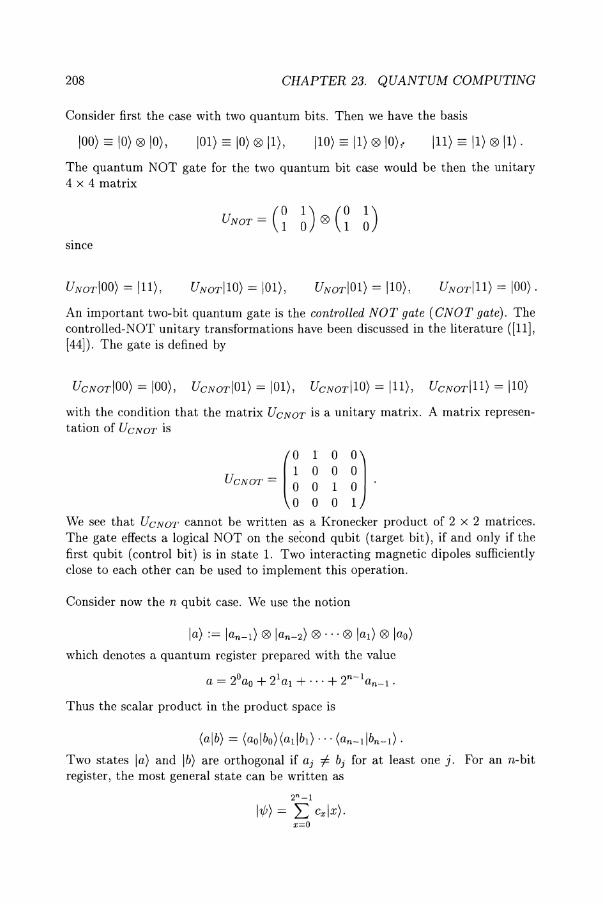
208 CHAPTER 23. QUANTUM COMPUTING
Consider first the case with two quantum bits. Then we have the basis
100) == 10) ® 10), 101) == 10) ® 11), 110) == 11) ® 10),. 111) == 11) ® 11) .
The quantum NOT gate for the two quantum bit case would be then the unitary 4 x 4 matrix
since
An important two-bit quantum gate is the controlled NOT gate (CNOT gate). The controlled-NOT unitary transformations have been discussed in the literature ([11], [44]). The gate is defined by
UcNoTIOO) = 100), UcNoTI01) = 101), UcNoTI1O) = 111), UcNoT I11) = 110)
with the condition that the matrix UCNOT is a unitary matrix. A matrix representation of UCNOT is
UCNOT = (~ ~ H). 000 1
We see that UCNOT cannot be written as a Kronecker product of 2 x 2 matrices. The gate effects a logical NOT on the second qubit (target bit), if and only if the first qubit (control bit) is in state 1. Two interacting magnetic dipoles sufficiently close to each other can be used to implement this operation.
Consider now the n qubit case. We use the notion
la) := lan-l) ® lan-2) ® ... ® lal) ® lao)
which denotes a quantum register prepared with the value
a = 2oao + 21al + ... + 2n - 1an_l .
Thus the scalar product in the product space is
(alb) = (aolbo)(allb1)··· (an-llbn- 1) .
Two states la) and Ib) are orthogonal if aj :j:. bj for at least one j. For an n-bit register, the most general state can be written as
2n-l
I'l/J) = L cxlx). x=o
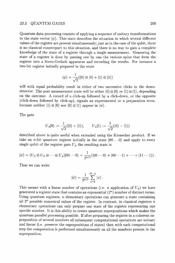
23.3. QUANTUM GATES 209
Quantum data processing consists of applying a sequence of unitary transformations to the state vector 11;0). This state describes the situation in which several different values of the register are present simultaneously; just as in the case of the qubit, there is no classical counterpart to this situation, and there is no way to gain a complete knowledge of the state of a register through a single measurement. Measuring the state of a register is done by passing one by one the various spins that form the register into a Stern-Gerlach apparatus and recording the results. For instance a two-bit register initially prepared in the state
11;0) = ~(IO) 010) + 11) 011))
will with equal probability result in either of two successive clicks in the downdetector. The post measurement state will be either 10) 010) or 11) 011), depending on the outcome. A record of a click-up followed by a click-down, or the opposite (click-down followed by click-up), signals an experimental or a preparation error, because neither 11) 010) nor 10) 011) appear in 11;0)·
The gate
described above is quite useful when extended using the Kronecker product. If we take an n-bit quantum register initially in the state 100 ... 0) and apply to every single qubit of the register gate U A the resulting state is
1 11;0) = (U A 0 U A 0 ... 0 U A) 100 ... 0) = ~ (100 ... 0) + 100 ... 1) + ... + 111 ... 1) ) .
2n / 2
Thus we can write
This means with a linear number of operations (i.e. n application of U A) we have generated a register state that contains an exponential (2n) number of distinct terms. Using quantum registers, n elementary operations can generate a state containing all 2n possible numerical values of the register. In contrast, in classical registers n elementary operations can only prepare one state of the register representing one specific number. It is this ability to create quantum superpositions which makes the quantum parallel processing possible. If after preparing the register in a coherent superposition of several numbers all subsequent computational operations are unitary and linear (i.e. preserve the superpositions of states) then with each computational step the computation is performed simultaneously on all the numbers present in the superposition.
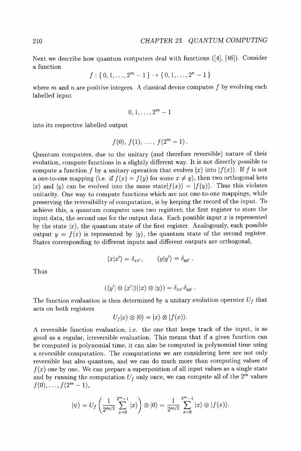
210 CHAPTER 23. QUANTUM COMPUTING
Next we describe how quantum computers deal with functions ([4], [46]). Consider a function
1 : {O, 1, ... , 2m - I} -+ {O, 1, ... , 2n - 1 }
where m and n are positive integers. A classical device computes 1 by evolving each labelled input
0,1, ... , 2m -1
into its respective labelled output
1(0),/(1), ... , 1(2m - 1).
Quantum computers, due to the unitary (and therefore reversible) nature of their evolution, compute functions in a slightly different way. It is not directly possible to compute a function 1 by a unitary operation that evolves Ix) into I/(x)). If 1 is not a one-to-one mapping (i.e. if I(x) = I(y) for some x =/: y), then two orthogonal kets Ix) and Iy) can be evolved into the same statelf(x)) = If(y)). Thus this violates unitarity. One way to compute functions which are not one-to-one mappings, while preserving the reversibility of computation, is by keeping the record of the input. To achieve this, a quantum computer uses two registers; the first register to store the input data, the second one for the output data. Each possible input x is represented by the state Ix), the quantum state of the first register. Analogously, each possible output y = I(x) is represented by Iy), the quantum state of the second register. States corresponding to different inputs and different outputs are orthogonal,
(yly') = byy' .
Thus
((y'l ® (x'I)(lx) ® Iy)) = bxx'byy' .
The function evaluation is then determined by a unitary evolution operator Uf that acts on both registers
Uflx) ® 10) = Ix) ® I/(x)).
A reversible function evaluation, i.e. the one that keeps track of the input, is as good as a regular, irreversible evaluation. This means that if a given function can be computed in polynomial time, it can also be computed in polynomial time using a reversible computation. The computations we are considering here are not only reversible but also quantum, and we can do much more than computing values of I(x) one by one. We can prepare a superposition of all input values as a single state and by running the computation UI only once, we can compute all of the 2m values 1(0), ... , 1(2m - 1),
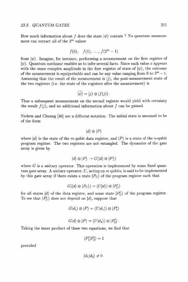
23.3. QUANTUM GATES 211
How much information about 1 does the state I'l/J) contain? No quantum measurement can extract all of the 2m values
1(0), 1(1), . .. , 1(2m - 1)
from I'l/J). Imagine, for instance, performing a measurement on the first register of I'l/J). Quantum mechanic enables us to infer several facts. Since each value x appears with the same complex amplitude in the first register of state of I'l/J), the outcome of the measurement is equiprobable and can be any value ranging from 0 to 2m - 1. Assuming that the result of the measurement is Ij), the post-measurement state of the two registers (Le. the state of the registers after the measurement) is
I'l/J) = Ij) ® If(j)) .
Thus a subsequent measurement on the second register would yield with certainty the result l(j), and no additional information about 1 can be gained.
Nielsen and Chuang [46) use a different notation. The initial state is assumed to be of the form
Id) ® IP)
where Id) is the state of the m-qubit data register, and IP) is a state of the n-qubit program register. The two registers are not entangled. The dynamics of the gate array is given by
Id) ® IP) -+ G(ld) ® IP))
where G is a unitary operator. This operation is implemented by some fixed quantum gate array. A unitary operator, U, acting on m qubits, is said to be implemented by this gate array if there exists a state IPu) of the program register such that
G(ld) ® IPu)) = (Uld)) ® IP~)
for all states Id) of the data register, and some state IP&) of the program register. To see that JP&) does not depend on Id), suppose that
Taking the inner product of these two equations, we find that
(P{IP~) = 1
provided
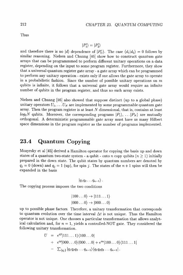
212 CHAPTER 23. QUANTUM COMPUTING
Thus
IP;) = IP~)
and therefore there is no Id) dependence of IPb). The ease (d1 Id2 ) = 0 follows by similar reasoning. Nielsen and Chuang [46] show how to construct quantum gate arrays that can be programmmed to perform different unitary operations on a data register, depending on the input to some program register. Furthermore, they show that a universal quantum register gate array - a gate array which can be programmed to perform any unitary operation - exists only if one allows the gate array to operate in a probabilistic fashion. Since the number of possible unitary operations on m qubits is infinite, it follows that a universal gate array would require an infinite number of qubits in the program register, and thus no such array exists.
Nielsen and Chuang [46] also showed that suppose distinct (up to a global phase) unitary operators U1 , ... UN are implemented by some programmable quantum gate array. Then the program register is at least N dimensional, that is, contains at least log2N qubits. Moreover, the corresponding programs IFI), .. . IPN ) are mutually orthogonal. A deterministic programmable gate array must have as many Hilbert space dimensions in the program register as the number of programs implemented.
23.4 Quantum Copying
Mozyrsky et al [45] derived a Hamilton operator for copying the basis up and down states of a quantum two-state system - a qubit - onto n copy qubits (n 2 1) initially prepared in the down state. The qubit states by quantum numbers are denoted by qj = 0 (down) and Qj = 1 (up), for spin j. The states of the n + 1 spins will then be expanded in the basis
Iqlq2 ... qn-l) .
The copying process imposes the two conditions
1100 ... 0) -+ 1111. .. 1)
1000 ... 0) -+ 1000 ... 0)
up to possible phase factors. Therefore, a unitary transformation that corresponds to quantum evolution over the time interval fit is not unique. Thus the Hamilton operator is not unique. One chooses a particular transformation that allows analytical calculation and, for n = 1, yields a controlled-NOT gate. They considered the following unitary transformation.
U ei ,Bll11 ... 1)(100 ... 01
+ eiPIOOO ... 0)(000 ... 01 + ei"II00 ... 0)(111 ... 11
I:{qj} Iqlq2q3 ... qn-l) (qlq2q3 ... qn-ll·
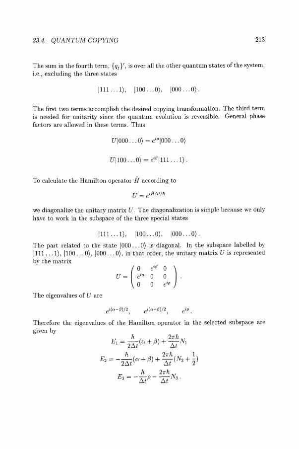
23.4. QUANTUM COPYING 213
The sum in the fourth term, {qj}', is over all the other quantum states of the system, i.e., excluding the three states
1111. .. 1), 1100 ... 0), 1000 ... 0).
The first two terms accomplish the desired copying transformation. The third term is needed for unitarity since the quantum evolution is reversible. General phase factors are allowed in these terms. Thus
UIOOO . .. 0) = eipIOOO ... 0)
_ i{J U1100 . .. 0) - e 1111 ... 1) .
To calculate the Hamilton operator iI according to
we diagonalize the unitary matrix U. The diagonalization is simple because we only have to work in the subspace of the three special states
1111 ... 1),1100 ... 0),1000 ... 0).
The part related to the state 1000 ... 0) is diagonal. In the subspace labelled by 1111 ... 1), 1100 ... 0), 1000 ... 0), in that order, the unitary matrix U is represented by the matrix
( 0 ei{J 0 )
U = eia 0 0. . o 0 e'P
The eigenvalues of U are
ei (a-{J)/2 , ei (a+{J)/2 ,
Therefore the eigenvalues of the Hamilton operator in the selected subspace are given by
Ii 27r1i El = 2~t (a + (3) + ~t Nl
Ii 27r1i 1 E2 = - 2~t (a + (3) + ~t (N2 + "2)
Ii 27r1i E3 = - ~tP - ~t N3 .
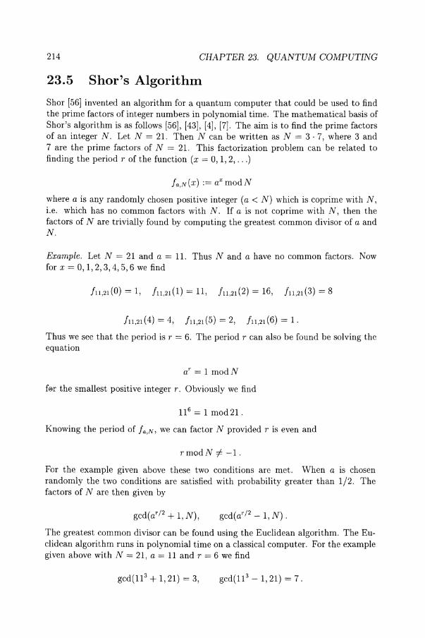
214 CHAPTER 23. QUANTUM COMPUTING
23.5 Shor's Algorithm
Shor [56] invented an algorithm for a quantum computer that could be used to find the prime factors of integer numbers in polynomial time. The mathematical basis of Shor's algorithm is as follows [56], [43], [4], [7]. The aim is to find the prime factors of an integer N. Let N = 21. Then N can be written as N = 3·7, where 3 and 7 are the prime factors of N = 21. This factorization problem can be related to finding the period r of the function (x = 0,1,2, ... )
1a,N(X):= aXmodN
where a is any randomly chosen positive integer (a < N) which is coprime with N, i.e. which has no common factors with N. If a is not coprime with N, then the factors of N are trivially found by computing the greatest common divisor of a and N.
Example. Let N = 21 and a = 11. Thus N and a have no common factors. Now for x = 0,1,2,3,4,5,6 we find
111,21(0) = 1, 111,21(1) = 11, 111,21(2) = 16, 111,21(3) = 8
111,21(4) = 4, 111,21(5) = 2, 111,21(6) = 1.
Thus we see that the period is r = 6. The period r can also be found be solving the equation
ar = 1 modN
fElr the smallest positive integer r. Obviously we find
116 = 1 mod21.
Knowing the period of 1a,N, we can factor N provided r is even and
rmodN -=1= -1.
For the example given above these two conditions are met. When a is chosen randomly the two conditions are satisfied with probability greater than 1/2. The factors of N are then given by
gcd(a r / 2 + 1, N), gcd(ar / 2 -1,N).
The greatest common divisor can be found using the Euclidean algorithm. The Euclidean algorithm runs in polynomial time on a classical computer. For the example given above with N = 21, a = 11 and r = 6 we find
gcd(113 + 1,21) = 3, gcd(113 -1,21) = 7.
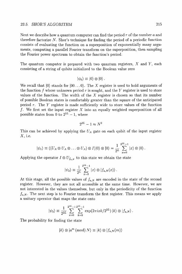
23.5. SHOR'S ALGORITHM 215
Next we describe how a quantum computer can find the period r of the number a and therefore factorize N. Shor's technique for finding the period of a periodic function consists of evaluating the function on a superposition of exponentially many arguments, computing a parallel Fourier transform on the superposition, then sampling the Fourier power spectrum to obtain the function's period.
The quantum computer is prepared with two quantum registers, X and Y, each consisting of a string of qubits initialized to the Boolean value zero
l1/Jo) == 10) ® 10) .
We recall that 10) stands for 100 ... 0). The X register is used to hold arguments of the function f whose unknown period r is sought, and the Y register is used to store values of the function. The width of the X register is chosen so that its number of possible Boolean states is comfortably greater than the square of the anticipated period r. The Y register is made sufficiently wide to store values of the function f. We first set the input register X into an equally weighted superposition of all possible states from 0 to 22L - 1, where
22L -1 ~ N 2
This can be achieved by applying the UA gate on each qubit of the input register X, i.e.
1 22L_1
11/J1) == ((UA ® UA ® .. , ® UA ) ® 1)10) ® 10) = 2L L Ix) ® 10) . x=O
Applying the operator I ® Ufa,N to this state we obtain the state
1 22L_1
11/J2) == 2L L Ix) ® Ifa,N(x)). x=O
At this stage, all the possible values of fa,N are encoded in· the state of the second register. However, they are not all accessible at the same time. However, we are not interested in the values themselves, but only in the periodicity of the function fa,N' The next step is to Fourier transform the first register. This means we apply a unitary operator that maps the state onto
1 22L_122L_1
11/J3) == 22L L L exp(27rixk/22L) Ik) ® Ifa,N)' x=O k=O
The probability for finding the state
Ik) ® lam (mod) N) == Ik) ® Ifa,N(m))
216 CHAPTER 23. QUANTUM COMPUTING
is
P(k, am (mod) N) ~ 12:L "/f"m ""p(2~ixk/2'L) , where the sum is over all numbers 0 S; x S; 22£ - 1 such that
aX = am (modN).
To find P we calculate the dual state of Ik) ®lfa,N(m)). Then we take the scalar product with IW3). The sum can be transformed into
11 [(22L-l-m)/r] 12
P(k, am mod N) = 2L L exp(21fib{rk h2L /22L ) 2 b=O
where {rk h2L is an integer in the interval
which is congruent to
rk (mod 22£ - 1) .
The above probability has well defined peaks if {rkh2L is small (less than r), i.e., if rk is a mUltiple of 22L
rk = d22L
for some d < N. Thus, knowing L and therefore 22L and the fact that the position of the peaks k will be close to numbers of the form d22L / r, we can find the period r using continuous fraction techniques. To explicitly construct the unitary evolution that takes the state IW1) into the state IW2) is a rather nontrivial task [43].
Chapter 24
Lebesgue Integration and Stieltjes Integral
In this chapter we give a short introduction to Lebesgue integration and Stieltjes integral (Halmos [27], Howson [29]). The Lebesgue integral plays a central role in the Hilbert spaces L2(M) (see chapter 1). The Stieltjes integral is important for the spectral representation (see chapter 4).
Let R be extended reals. A function J1. : C -+ R, whose domain is a non-empty class C of subsets of some set X (assumed to include the empty set 0) and whose codomain is the extended real number system, is said to be a finitely additive set function if
J1.(0) = 0
and if for every collection EI, ... ,En of pairwise disjoint sets of C such that their union
n
UEi i=1
belongs to C we have
J1. (Q Ei) = ~ J1.(Ei).
An additive set function J1. is said to be count ably additive, completely additive, or a-additive if for every countable collection E1 , E2 , . •. of pairwise disjoint sets of C whose union is in C, we have
217
W.-H. Steeb, Hilbert Spaces, Wavelets, Generalised Functions and Modern Quantum Mechanics© Kluwer Academic Publishers 1998
218 CHAPTER 24. LEBESGUE INTEGRATION AND STIELT JES INTEGRAL
A measure is defined to be a non-negative, countably additive set function (i.e. a a-additive set function with codomain {x E Rlx 2: o}).
If p, is a measure on a ring R, then a set E E R is said to have finite measure if p,(E) E R. E is said to have a-finite measure if there is a sequence (En) of sets of finite measure in R such that
i=l
If every set in R has finite (a-finite) measure, then p, is said to be finite (or a-finite) on R. If R is an algebra of sets, then p, is called totally finite (totally a-finite).
Given two classes C and D of subsets of X satisfying C c D, and two set functions p" v defined upon C and D respectively we say that v is an extension of p, and that p, is a restriction of v if for all E E C we have
p,(E) = v(E).
A non-empty class C of sets is said to be hereditary if
(E E C and FeE) :::} F E C.
A set function p,* : C ---+ R is said to be monotone if
(E, FE C and E c F) :::} p,*(E) :::; p,*(F).
A non-negative set function
p,* : C ---+ { x E R : x 2: 0 }
is said to be subadditive if
(E, F, E U FE C) :::} p,*(E U F) :::; p,*(E) + p,*(F).
A subadditive set function p,' is countably subadditive if, for every sequence (Ei) of sets of C whose union is also in C,
A monotone, countably subadditive set function p,* defined on a hereditary a-ring 11. and such that p,*(0) = 0 is known as an outer measure.
219
Next we introduce the Lebesgue measure. We define an interval Rn to be a set of the form
{ (XI, X2, ... ,xn ) : ai * Xi t bi , i = 1,2, ... ,n}
where * and t denote either < or:::;. We also allow that ai = bi and include the empty set amongst the set of intervals.
If A is the union of a finite number of such intervals, we say that it is an elementary set.
The class of all elementary sets is a ring en. It can be shown that if A E en then A can be presented as the finite union of pairwise disjoint intervals
If then we denote the content of an interval I by
n
m(I) = II (bi - ai) i=1
we can define a non-negative additive set function m : en -+ R by
N
m(A) = L m(Ij). j=1
In the cases n = 1,2, and 3, m is length, area and volume respectively.
Clearly en is not a (I-ring and does not contain all those subsets of Rn which are important in integration theory. Therefore we have to extend m to a larger class of sets.
We consider countable coverings of any set E c R n by open sets of R n ,
Such a covering, i.e. by a countable number of open sets, is called a Lebesgue covering. Let
00
m(E) := glb L m(Ai) i=1
where the glb is taken over all Lebesgue coverings of E. 'glb' stands for greatest lower bound. It can then be shown that in is an extension of m from en to the class of all subsets of Rn and that it is an outer measure on the (I-ring. in is known as the Lebesgue outer measure. Let A, BeRn. We define
d(A, B) := in(A~B)
220 CHAPTER 24. LEBESGUE INTEGRATION AND STIELT JES INTEGRAL
where L), denotes the symmetric difference of the sets A and B. We write Ai --+ A if A, Ai C R n (i = 1,2, ... ) and
.lim d(A, Ai) = o . • ~OO
If there is a sequence of sets of £n such that Ai --+ A, we say that A is finitely m-measurable and write A E MF(m). If A is the union of a countable collection of finitely m-measurable sets, then A is said to be m-measurable and we write A E M(m).
Obviously M(m) is a a-ring. Setting m(A) = m(A) for all A E M(m), we obtain an extension of m from £n to the class M(m). m is known as the Lebesgue measure on Rn and we say that an m-measurable set is Lebesgue measurable.
Example. All open sets ofRn and all closed sets ofRn belong to M(m). It follows that all Borel sets in Rn are Lebesgue measurable. ..
Notice that not all subsets of Rn are Lebesgue measurable (Howson [29]).
Definition. A set E for which m(E) = 0 is said to be a set of Lebesgue measure zero.
Example. Every countable set has Lebesgue measure zero. The converse, however, is not true. An example is the standard Cantor set. ..
The sets of measure zero form a a-ring. The term almost everywhere (a.e.) is used to mean 'except on a set of Lebesgue measure zero'. Every Lebesgue measurable set in R n can be presented as the union of a Borel set and a set of measure zero. All sets of Lebesgue measure zero are Lebesgue measurable.
Next we introduce measurable functions. We say that a set X is a measurable space (X, S) if there is a a-ring S of subsets of X such that uS = X. A measure space, (X, S, f.1-) is a measurable space together with a measure f.1- defined on S (the a-ring of measurable sets).
Example. (Rn, M(m), m) is a measure space. ..
Let f : X --+ R be a function defined on a measure space X. We say that f is measurable if the set
{x: f(x»a}
is measurable for all a E R.
A function f : X --+ R is said to be simple if there is a finite, pairwise disjoint class {El' ... ,En} of measurable sets and a finite set {at, ... ,an} of real numbers such
221
that f (x) = {O:i ~f X E E~ (i = 1, ... , n)
o If x tj. Ui=IEi.
Example. A simple function is the characteristic function XE of a measurable set E defined by
{ I if xEE XE(X) = 0 if x tj. E.
A simple function can, therefore, be presented in the form
n
f = LO:iXEi· i=1
Every measurable function is the limit of a sequence of simple functions and that if the function is non-negative, then the sequence can be chosen to be monotonically increasing.
Next we introduce integration. A simple function f on a measure space (X, S, fJ) is integrable if fJ(Ei) is finite for every i for which O:i is non-zero. The integral of f is defined by
where 0 x (+00) = O. If f is integrable, the value of the integral is finite.
Let E be a measurable set and f be an integrable simple function. Then we define the integral of f over E, written as
f fdfJ E
to be the integral of the product function XEf.
If f is a measurable, non-negative function we define the integral of f over E with respect to the measure fJ by
1 fdfJ := lub {I sdfJ }
where the lub is taken over all simple functions s such that 0 :::; s :::; f· f is said to be integrable over E if the integral is finite.
Alternatively, we can define
f fdfJ = lim f fndfJ n-+oo E E
222 CHAPTER 24. LEBESGUE INTEGRATION AND STIELT JES INTEGRAL
where (fn) is a monotone increasing sequence of simple functions such that fn -+ f. This limit is independent of the choice of sequence.
If f is any measurable function, then the functions
r =max(f,O)
and r = -min (1,0)
are also measurable and are non-negative. We can, therefore, form
f rd{t and f rd{t. E E
If at least one of these integrals is finite we define the integral of f over E, written f fd{t, to be E
f rd{t - f f-d{t. E E
If f f d{t is finite, we say that f is integrable (or summable) over E. E
In the special case when X = Rn, {t is the Lebesgue measure and S is the set of Lebesgue measurable functions, then it is usual to denote the integral- the Lebesgue integral - by
f f(x)dx E
rather than f f dm. E
Let us now give some examples. In the examples below, sets are considered as subsets of the interval [0, 1] with uniform Lebesgue measure {to
(1) Sp = countable union of points. Then {t(Sp) = O. This includes the rationals.
(2) Se = the usual Cantor set, obtained by deleting middle thirds. Again {t(Se) = O.
(3) SF = a fat fractal, constructed as follows. Starting from the interval [0,1], one deletes a fraction 1/nl. From the remaining two intervals, one deletes a fraction
1 -1-1 2(1 - n 1 )n2 .
At the k-th step, one has 2k intervals. In the (k + l)-th step, one deletes a fraction
k 2- k II(l -1)-1 - nl nk+l'
1=1
223
The Cantor set is the complement of this set in the interval [0,1]. For example, in the usual Cantor set, we have nk = 3. The Lebesgue measure of this set is
co
p,(Sp) = II(1-nk1) k=l
with the understanding that it is 0 if L: link diverges.
(4) SN = the set of noble reals, i.e. all real numbers x obtained from the golden mean
by an action of
1 a = -(V5 - 1)
2
aa+b SL(2,Z) : x = ca+d
where a, b, c, d are integers and
det (~ ~) = l.
As a countable union of points it has
(5) SD = Diophantine numbers of power p. A real number a satisfies a diophantine condition of order p, of for all rationals p/q
'Y la- plql2: p q
with some constant 'Y > O. One finds
if and only if p > 2.
(6) SL = Liouville numbers. A real number a is called a Liouville number, if it is not rational and if it is easy to approximate by rationals. Formally, there is a sequence (Pn/ qn)n=1,2, ... ,co such that
They are of measure zero
224 CHAPTER 24. LEBESGUE INTEGRATION AND STIELT JES INTEGRAL
Finally we give a short introduction to the Riemann-Stieltjes integral. We assume that the reader is familiar with the Riemann integral. Let f and a be bounded, real-valued functions defined upon a closed finite interval I = [a, b] of R (a -=1= b). Let
P := {xo, ... ,Xn }
be a partition of I and ti be a point of the subinterval [Xi-I, Xi]. A sum of the form
n
S(F, f, a) = 2: f(ti)(a(xi) - a(xi-l)) i=1
is called a Riemann-Stieltjes sum of f with respect to a. f is said to be Riemann integrable with respect to a on I if there exists A E R such that given any E > 0 there exists a partition FE of I for which, for all F finer than FE and for every choice of points t i , we have
IS(P, f, a) - AI < E-
If such an A exists, then it is unique and is known as the Riemann-Stieltjes integral of f with respect to a. f is known as the integrand and a the integrator. The integral is denoted by
b b
J fda or J f(x)da(x). a a
Bibliography
[1] Ablowitz M. J. and H. Segur, Solitons and the Inverse Scattering Transform, SIAM, Philadelphia, 1981.
[2] Arnold V. I., Mathematical Methods in Classical Mechanics, Springer-Verlag, New York, 1982.
[3] Balakrishnan A. V., Applied Functional Analysis, Second Edition SpringerVerlag, New York, 1981.
[4] Barenco A., "Quantum Physics and Computers", Contemporary Physics 37, 375-389, 1996.
[5] Bell J. S., Speakable and unspeakable in quantum mechanics, Cambridge University Press, Cambridge, 1989.
[6] Bender C. M. and T. T. Wu, "Anharmonic Oscillators", Physical Review 184, 1291~1299, 1969.
[7] Bennett H. C., "Quantum Information and Computation", Physics Today, October, 24~30, 1995.
[8] Berry M. V., "Quantal phase factors accompanying adiabatic changes", Proc. Royal Soc. London Ser. A392, 45-57, 1984.
[9] Berry M. V., The quantum phase, five years after in Geometric Phases in Physics, ed. F. Wilzcek and A. Shapere, World Scientific, Singapore, 1989.
[10] Berry M. V. and R. Lim, "The Born-Oppenheimer electric gauge force is repulsive near degeneracies", J. Phys. A: Math. Gen. 23, L655-L657, 1990.
[11] Cirac J. I. and P. Zoller, "Quantum Computations with Cold Trapped Ions", Physical Review Letters, 74, 4091 ~4094, 1995.
[12] Chan Y. T., Wavelet Basics, Kluwer Academic Publishers, Boston, 1995.
[13] Chui C. K., An Introduction to Wavelets, Academic Press, Boston, 1992.
225
[14] Collatz L., Functional Analysis and Numerical Mathematics, Academic Press, New York, 1966,
[15] Constantinescu F. and E. Magyari, Problems in Quantum Mechanics, Pergamon Press, Oxford, 1971.
[16] Debnath L. and P. Mikusinski, Introduction to Hilbert Spaces with Applications Academic Press, Boston, 1990.
[17] Dirac P. A. M., The Principles of Quantum Mechanics, Clarendon Press, Oxford, 1958.
[18] Eder G., Quantenmechanik, Bibliographisches Institut, Mannheim, 1968.
[19] Einstein A., B. Podolski and N. Rosen, "Can quantum mechanical description of reality be considered complete ?", Physical Review 47, 777-780, 1935.
[20] Elby A. and J. Bub, "'Ifiorthogonal uniqueness theorem and its relevance to the interpretation of quantum mechanics", Physical Review A, 49, 4213-4216, 1994.
[21] Everett III H., "Relative state formulation of quantum mechanics" Review of Modern Physics 29 454-462, 1957.
[22] Fliigge S., Practical Quantum Mechanics, Springer-Verlag, Berlin, 1974.
[23] Gardner C. S., J. M. Greene, M. D. Kruskal and R M. Miura, "Korteweg-de Vries equation and generalization. VI. Methods for exact solution", Communication in Pure and Applied Mathematics, 27, 97-133, 1974.
[24] Gasiorowicz S., Quantum Physics, Wiley, New York, 1974.
[25] Gelfand I. M and G. E. Shilov, Generalized Functions 1, Academic Press, Or-lando, 1964.
[26] Glimm J. and A. Jaffe, Quantum Physics, Springer-Verlag, New York, 1981.
[27] Halmos P. R, Measure Theory, van Nostrand, Princeton, 1966.
[28] Healey R, The philosophy of quantum mechanics, Cambridge University Press, Cambridge, 1990.
[29] Howson A. G., A handbook of terms used in algebra and analysis, Cambridge University Press, London, 1972.
226
[30] Kaiser G., A Friendly Guide to Wavelets, Birkhiiuser, Boston, 1994.
[31] Kato T., Perturbation Theory of Linear Operators, Springer-Verlag, Berlin, 1984.
[32] Klauder J. R. and B. Skagerstam, Coherent states - Applications in Physics and Mathematical Physics, World Scientific, Singapore, 1985.
[33] Kowalski K. and W.-H. Steeb, Carleman Linearization, World Scientific, Singapore 1991.
[34] Kummer M., "How to avoid secular terms in classical and quantum mechanics", II Nuovo Cimento lB, 123-148, 1971.
[35] Lamb G. L., Elements of Soliton Theory, Wiley, New York, 1980.
[36] Landau L. D. and E. M. Lifshitz, Quantum Mechanics, Pergamon Press, Oxford,1958.
[37] Louisell W. H., Quantum Statistical Properties of Radiation, Wiley, New York, 1973.
[38] Ludwig W. and C. Falter, Symmetries in Physics, Springer-Verlag, Berlin, 1988.
[39] Mavromatis H. A., Exercises in Quantum Mechanics, Reidel, Dordrecht, 1987.
[40] McDonald S. W. and A. N. Kaufman, "Spectrum and eigenfunctions for a Hamiltonian with stochastic trajectories", Physical Review Letters 42, 1189-1191,1979.
[41] Messiah A., Quantum Mechanics, Interscience, New York, 1961.
[42] Miller W., Symmetry Groups and Their Applications, Academic Press, New York,1972.
[43] Miquel C., J. P. Paz and R. Perazzo, "Factoring in a dissipative quantum computer" , Physical Review A 54, 2605-2613, 1996.
[44] Monroe C., D. M. Meekhof, B. E. King, W. M. Itano and D. J. Wineland, "Demonstration of a Fundamental Quantum Logic Gate" , Physical Review Letters, 75, 4714-4717, 1995.
[45] Mozyrsky D., V. Privman and M. Hillary, "A Hamiltonian for quantum copying" , Physics Letters A 226, 253-256, 1997.
[46] Nielsen M. A. and I. L. Chuang, "Programmable Quantum Gate Arrays", Physical Review Letters 79, 321-324, 1997.
227
[47] Prugovecki E., Quantum Mechanics in Hilbert Space, Second Edition, Academic Press, New York, 1981.
[48] Redhead M., Incompleteness, Nonlocality, and Realism Clarendon Press, Oxford, 1990.
[49] Richtmyer R. D., Principles of Advanced Mathematical Physics, Volume I, Springer-Verlag, New York, 1978.
[50] Sagdeev R. Z., D. A. Usikov and G. M. Zaslavsky, Nonlinear Physics, Harwood, Chur, 1988.
[51] Schiff L. 1., Quantum Mechanics, McGraw-Hill, New York, 1968.
[52] Schommers W. (Editor), Quantum Theory and Picture of Reality, SpringerVerlag, Berlin, 1989.
[53] Schri:idinger E., "Discussion of Probability Relations Between Separated Systems", Proceedings of the Cambridge Philosophical Society, 31, 555-563, 1935.
[54] Sewell G. L., Quantum Theory of Collective Phenomena, Clarendon Press, Oxford, 1986.
[55] Shanley P. E., "Spectral Properties of the Scaled Anharmonic Oscillator", Annals of Physics (New York) 186, 292-324, 1988.
[56] Shor P. W., "Procedeedings of the 35th Annual Symposium on the Foundations of Computer Science", edited by S. Goldwasser (Los Alamitos, CA: IEEE Compuer Society Press), p. 124, 1994.
[57] Simon B., "Coupling Constant Analyticity for the Anharmonic Oscillator", Annals of Physics (New York) 58,76-136,1970.
[58] Stakgold 1., Boundary Value Problems of Mathematical Physics, Volume I, MacMillan, New York 1967.
[59] Steeb W. H., Quantum Mechanics using Computer Algebra, World Scientific, Singapore, 1994.
[60] Steeb W. H., Continuous Symmetries, Lie Algebras and Differential Equations, World Scientific, Singapore, 1996.
[61] Steeb W. H., Problems and Solutions in Theoretical and Mathematical Physics, Volume I, World Scientific, Singapore, 1996.
[62] Steeb W. H., Problems and Solutions in Theoretical and Mathematical Physics, Volume II, World Scientific, Singapore, 1996.
228
[63] Steeb W.-H., Matrix Calculus and Kronecker Product with Applications and C++ Programs, World Scientific, Singapore, 1997.
[64] ter Haar D., Selected Problems in Quantum Mechanics, Infosearch, London, 1964.
[65] Vigier J. P., "Non-locality Causality and Aether in Quantum Mechanics", Astronomische Nachrichten, 303, 55-80, 1982.
[66] Vinet L., "Symmetries and Berry Connections" in Symmetries and Nonlinear Phenomena editors D. Levi and P. Winternitz, World Scientific, Singapore, 1988.
[67] Vladimirov V. S., Equations of Mathematical Physics, Dekker, New York, 1971.
[68] Weidmann J., Linear Operators in Hilbert Space, Springer-Verlag, New York, 1980.
[69] Yosida K., Functional Analysis, Springer-Verlag, Berlin, 1978.
229
Index
Abelian group, 109 Adiabatic approximation, 189 Adiabatic theorem, 189 Adjoint operator, 32 Algebraic tensor product, 12 Almost everywhere, 220 Amost everywhere, 18 Angular momentum, 141 Angular momentum operator, 72 Anharmonic oscillator, 176 Annihilation operator, 44 Anti-commutation relation, 139 Averaging method, 82
Banach space, 3 Basis degeneracy problem, 196 Berry connection, 191 Berry's phase, 190 Bessel differential equation, 97 Bessel functions, 98 Biorthogonal decomposition theorem,
203 Born amplitude, 185 Born-Oppenheimer approximation, 191 Bose annihinlation operator, 128 Bose coherent state, 135 Bose creation operator, 128 Bounded, 31 Bra vector, 14
Casimir operator, 144 Cauchy principal value, 53, 57 Cauchy sequence, 3 Center of mass position vector, 150 Character table, 114 Characteristic equation, 38 Characteristic funtion, 221 CNOT gate, 208
231
Coherent states, 135 Commutative group, 109 Commutator, 47 Commute, 109 Compatible, 120 Complementary, 120 Complete, 3 Completeness relation, 147 Confluent series, 152 Conjugacy classes, 110 Conjugate, 110 Continuous spectrum, 37 Controlled NOT gate, 208 Converge strongly, 4, 35 Converge uniformly, 35 Converge weakly, 4, 35 Convolution, 19 Convolution theorem, 21 Creation operator, 44 Cyclotron frequency, 67
Delta function, 53 Density matrix, 35 Deviations, 121 Differential cross section, 184 Dilation, 25 Dirac notation, 14 Dirac spin matrices, 105 Direct product, 55 Dirichlet boundary condition, 93 Discrete spectrum, 45 Displaced harmonic oscillator, 137 Distance, 2 Domain, 31 Dyadic product, 14 Dyadic translation, 25 Dyadic wavelet, 28
Eigenspace, 37 Eigenvalue, 37 Eigenvalue equation, 86 Eigenvector, 37 Even function, 113
Fat fractal, 222 Fermi annihilation operators, 139 Fermi creation operators, 139 First integral, 65 Form factor, 186 Fourier expansion, 9 Fourier transform, 20 Fredholm-type integral equation, 184 Free particle, 88 Functional, 52 Fundamental solution, 58
Gamma function, 147 Gelfand-Levitan-Marchenko integral equa-
tion, 168 Generalized eigenvector, 59 Generalized function, 52 Generating function, 127 Group, 109
Haar function, 25 Hamilton equations of motion, 63 Hamilton function, 63 Harmonic Oscillator, 123 Heisenberg model, 106 Heisenberg pciture, 77 Heisenberg picture, 73 Heisenberg's uncertainty relation, 120 Helium atom, 179 Helmholtz equation, 93 Hermite polynomials, 12, 126 Hilbert space, 1, 3
Incident flux, 184 Inequality of Schwarz, 9 Inner product, 1 Integral wavelet transform, 26 Interaction picture, 78 Interaction state vector, 78 Inverse formula, 27
232
Inverse Fourier transform, 22 Invertible transformation, 149 Irreducible, 114 Isomorphic, 142
Jacobi identity, 142
Ket vector, 14 Korteweg-de Vries equation, 165 Kronecker delta, 8 Kronecker product, 103 Kummer equation, 151
Laguerre polynomials, 12 Lax pair method, 165 Lebesgue integration, 217 Lebesgue measure, 219, 220 Lebesgue outer measure, 219 Lebesgue square-integrable functions,
6 Legendre polynomials, 10 Lie algebra, 141, 142 Lie subalgebra, 142 Logical gates, 205
M¢ller operator, 188 Measurable, 220 Measure, 218 Modified Laguerre polynomials, 155 Multiplicity, 37
Norm, 31 Normed space, 2 Null function, 18 N ullspace, 33
Odd function, 113 One-parameter group, 35 Ortho states, 182 Orthogonal, 2 Orthogonal complement, 7 Orthogonal sequence, 8
Para states, 182 Parallelogram identity, 15 Parity operator, 110 Parseval's relation, 9
Partial waves, 186 Particle-number operator, 45 Pauli exclusion principle, 182 Pauli principle, 139 Pauli spin matrices, 101 Plancherel theorem, 23 Plane wave solution, 184 Point spectrum, 37 Poisson bracket, 65, 142 Polar coordinates, 96 Polarization indentity, 23 Positive, 33 Power series ansatz, 125 Pre-Hilbert space, 1 Principal quantum number, 155 Probability flux, 157 Product ansatz, 85 Projection operator, 33
Quantization, 72 Quantum bit, 206 Quantum gates, 207 Quantum register, 207 Qubit, 206
Rademacher function, 16 Radial equation, 151, 186 Radial quantum number, 152, 155 Rayleigh-Schrodinger perurbation the-
ory, 171 Reduced mass, 150, 186 Reducible, 114 Reflection coefficient, 157 Residual spectrum, 37 Resolvent, 37 Resolvent set, 37 Resonance phenomena, 163 Riemann-Stieltjes integral, 224 Rotator, 89
S-matrix, 81 Scalar product, 1 Scattering amplitude, 185 Schrodinger equation, 70 Schrodinger picture, 73, 77 Secular equation, 38
233
Secular terms, 81 Self-adjoint, 32 Separable, 7 Separation ansatz, 85 Sine-Gordon equation, 170 Spectral theorem, 46 Spectral theory, 37 Spectrum, 37 Spherical coordinates, 143 Spherical harmonics, 11 Spin matrices, 106 Squeezed state, 138 Step function, 53 Stieltjes integral, 217 Subspace, 7
Tensor product, 12, 36, 55 Test functions, 51 Time average, 124 Time-energy uncertainty relation, 120 Time-ordered product of operators, 80 Total cross section, 184 Trace, 6, 35 Translation operator, 35 Transmission coefficient, 157 Triangle inequality, 9 Truth table, 205 Tunnel effect, 163
Uncertainties, 119 Uncertainty relation, 119 Unitary operator, 34
Variational principle, 180
Wavelet coefficients, 26 Wavelet series, 26 Wavelet transform, 17 Wavelets, 24 Wigner phase space density, 133 Wigner-Weyl formalism, 134 Windowed Fourier transform, 17, 24
Other Mathematics and Its Applications titles of interest:
F. Neuman: Global Properties of Linear Ordinary Differential Equations. 1992, 320 pp. ISBN 0-7923-1269-4
A. Dvureeenskij: Gleason's Theorem and its Applications. 1992, 334 pp. ISBN 0-7923-1990-7
D.S. Mitrinovie, J.E. Peearie and A.M. Fink: Classical and New Inequalities in Analysis. 1992,740 pp. ISBN 0-7923-2064-6
H.M. Hapaev: Averaging in Stability Theory. 1992,280 pp. ISBN 0-7923-1581-2
S. Gindinkin and L.R. Volevich: The Method of Newton's Polyhedron in the Theory of PDE's.1992,276pp. ISBN 0-7923-2037-9
Yu.A. Mitropolsky, A.M. Samoilenko and 0.1. Martinyuk: Systems of Evolution Equations with Periodic and Quasiperiodic Coefficients. 1992,280 pp. ISBN 0-7923-2054-9
LT. Kiguradze and T.A. Chanturia: Asymptotic Properties of Solutions of Nonautonomous Ordinary Differential Equations. 1992,332 pp. ISBN 0-7923-2059-X
V.L. Kocie and G. Ladas: Global Behavior of Nonlinear Difference Equations of Higher Order with Applications. 1993, 228 pp. ISBN 0-7923-2286-X
S. Levendorskii: Degenerate Elliptic Equations. 1993,445 pp. ISBN 0-7923-2305-X
D. Mitrinovie and J.D. Keckicl: The Cauchy Method of Residues, Volume 2. Theory and Applications. 1993,202 pp. ISBN 0-7923-2311-8
R.P. Agarwal and P.J.Y Wong: Error Inequalities in Polynomial Interpolation and Their Applications. 1993,376 pp. ISBN 0-7923-2337-8
A.G. Butkovskiy and L.M. Pustyl'nikov (eds.): Characteristics of Distributed-Parameter Systems. 1993, 386 pp. ISBN 0-7923-2499-4
B. Stemin and V. Shatalov: Differential Equations on Complex Manifolds. 1994, 504 pp. ISBN 0-7923-2710-1
S.B. Yakubovieh and Y.F. Luchko: The Hypergeometric Approach to Integral Transforms and Convolutions. 1994, 324pp. ISBN 0-7923-2856-6
C. Gu, X. Ding and C.-C. Yang: Partial Differential Equations in China. 1994, 181 pp. ISBN 0-7923-2857-4
V.G. Kravchenko and G.S. Litvinehuk: Introduction to the Theory of Singular Integral Operators with Shift. 1994, 288 pp. ISBN 0-7923-2864-7
A. Cuyt (ed.): Nonlinear Numerical Methods and RationalApproximationii. 1994,446 pp. ISBN 0-7923-2967-8
G. Gaeta: Nonlinear Symmetries and Nonlinear Equations. 1994,258 pp. ISBN 0-7923-3048-X
Other Mathematics and Its Applications titles of interest:
V.A. Vassiliev: Ramified Integrals, Singularities and Lacunas. 1995, 289 pp. ISBN 0-7923-3193-1
N.1a. Vilenkin and A.V. Klimyk: Representation of Lie Groups and Special Functions. Recent Advances. 1995, 497 pp. ISBN 0-7923-3210-5
Yu. A Mitropolsky and A.K. Lopatin: Nonlinear Mechanics, Groups and Symmetry. 1995, 388 pp. ISBN 0-7923-3339-X
R.P. Agarwal and P.Y.H. Pang: Opial Inequalities with Applications in Differential and Difference Equations. 1995,393 pp. ISBN 0-7923-3365-9
A.G. Kusraev and S.S. Kutateladze: Subdifferentials: Theory and Applications. 1995, 408 pp. ISBN 0-7923-3389-6
M. Cheng, D.-G. Deng, S. Gong and c.-C. Yang (eds.): Harmonic Analysis in China. 1995, 318 pp. ISBN 0-7923-3566-X
M.S. Livsic, N. Kravitsky, A.S. Markus and V. Vinnikov: Theory of Commuting Nonselfadjoint Operators. 1995, 314 pp. ISBN 0-7923-3588-0
A.1. Stepanets: Classification and Approximation of Periodic Functions. 1995, 360 pp. ISBN 0-7923-3603-8
C.-G. Ambrozie and F.-H. Vasilescu: Banach Space Complexes. 1995,205 pp. ISBN 0-7923-3630-5
E. Pap: Null-Additive Set Functions. 1995,312 pp. ISBN 0-7923-3658-5
c.J. Colboum and E.S. Mahmoodian (eds.): Combinatorics Advances. 1995,338 pp. ISBN 0-7923-3574-0
V.G. Danilov, V.P. Maslov and K.A. Volosov: Mathematical Modelling of Heat and Mass Transfer Processes. 1995, 330 pp. ISBN 0-7923-3789-1
A Laurincikas: Limit Theorems for the Riemann Zeta-Function. 1996, 312 pp. ISBN 0-7923-3824-3
A Kuzhel: Characteristic Functions and Models of Nonself-Adjoint Operators. 1996, 283 pp. ISBN 0-7923-3879-0
G.A. Leonov, I.M. Burkin and AI. Shepeljavyi: Frequency Methods in Oscillation Theory. 1996,415 pp. ISBN 0-7923-3896-0
B. Li, S. Wang, S. Yan and c.-C. Yang (eds.): FunctionalAnalysis in China. 1996,390 pp. ISBN 0-7923-3880-4
P.S. Landa: Nonlinear Oscillations and Waves in Dynamical Systems. 1996,554 pp. ISBN 0-7923-3931-2
A.1. Jerri: Linear Difference Equations with Discrete Transform Methods. 1996,462 pp. ISBN 0-7923-3940-1
Other Mathematics and Its Applications titles of interest:
I. Novikov and E. Semenov: Haar Series and Linear Operators. 1997,234 pp. ISBN 0-7923-4006-X
L. Zhizhiashvi1i: Trigonometric Fourier Series and Their Conjugates. 1996, 312 pp. ISBN 0-7923-4088-4
R.G. Buschman: Integral Transformation, Operational Calculus, and Generalized Functions. 1996,246 pp. ISBN 0-7923-4183-X
v. Lakshmikantham, S. Sivasundaram and B. Kaymakcalan: Dynamic Systems on Measure Chains. 1996,296 pp. ISBN 0-7923-4116-3
D. Guo, V. Lakshmikantham and X. Liu: Nonlinear Integral Equations in Abstract Spaces. 1996,350 pp. ISBN 0-7923-4144-9
Y. Roitberg: Elliptic Boundary Value Problems in the Spaces of Distributions. 1996,427 pp. ISBN 0-7923-4303-4
Y. Komatu: Distortion Theorems in Relation to Linear Integral Operators. 1996, 313 pp. ISBN 0-7923-4304-2
A.G. Chentsov: Asymptotic Attainability. 1997,336 pp. ISBN 0-7923-4302-6
S.T. Zavalishchin and A.N. Sesekin: Dynamic Impulse Systems. Theory and Applications. 1997,268 pp. ISBN 0-7923-4394-8
U. Elias: Oscillation Theory of Two-Term Differential Equations. 1997,226 pp. ISBN 0-7923-4447-2
D. O'Regan: Existence Theory for Nonlinear Ordinary Differential Equations. 1997,204 pp. ISBN 0-7923-4511-8
Yu. Mitropolskii, G. Khoma and M. Gromyak: Asymptotic Methodsfor Investigating Quasiwave Equations of Hyperbolic Type. 1997,418 pp. ISBN 0-7923-4529-0
R.P. Agarwal and P.J.Y. Wong: Advanced Topics in Difference Equations. 1997,518 pp. ISBN 0-7923-4521-5
N.N. Tarkhanov: The Analysis of Solutions of Elliptic Equations. 1997,406 pp. ISBN 0-7923-4531-2
B. Riecan and T. Neubrunn: Integral, Measure, and Ordering. 1997,376 pp. ISBN 0-7923-4566-5
N.L. Gol'dman: Inverse Stefan Problems. 1997,258 pp. ISBN 0-7923-4588-6
S. Singh, B. Watson and P. Srivastava: Fixed Point Theory and Best Approximation: The KKM-map Principle. 1997,230 pp. ISBN 0-7923-4758-7
A. Pankov: G-Convergence and Homogenization of Nonlinear Partial Differential Operators. 1997,263 pp. ISBN 0-7923-4720-X
Other Mathematics and Its Applications titles of interest:
S. Hu and N.S. Papageorgiou: Handbook of Multi valued Analysis. Volume I: Theory. 1997, 980 pp. ISBN 0-7923-4682-3 (Set of 2 volumes: 0-7923-4683-1)
L.A. Sakhnovich: Interpolation Theory and Its Applications. 1997,216 pp. ISBN 0-7923-4830-0
G.V. Milovanovic: Recent Progress in Inequalities. 1998,531 pp. ISBN 0-7923-4845-1
V.V. Filippov: Basic Topological Structures of Ordinary Differential Equations. 1998, 530 pp. ISBN 0-7293-4951-2
S. Gong: Convex and Starlike Mappings in Several Complex Variables. 1998, 208 pp. ISBN 0-7923-4964-4
A.B. Kharazishvili: Applications of Point Set Theory in Real Analysis. 1998, 244 pp. ISBN 0-7923-4979-2
R.P. Agarwal: Focal Boundary Value Problems for Differential and Difference Equations. 1998, 300 pp. ISBN 0-7923-4978-4
D. Przeworska-Rolewicz: Logarithms andAntilogarithms. An Algebraic Analysis Approach. 1998,358 pp. ISBN 0-7923-4974-1
Yu. M. Berezansky and A.A. Kalyuzhnyi: Harmonic Analysis in Hypercomplex Systems. 1998,493 pp. ISBN 0-7923-5029-4
V. Lakshmikantham and A.S. Vatsala: Generalized Quasilinearizationfor Nonlinear Problems. 1998, 286 pp. ISBN 0-7923-5038-3
V. Barbu: Partial Differential Equations and Boundary Value Problems. 1998,292 pp. ISBN 0-7923-5056-1
J. P. Boyd: Weakly Nonlocal Solitary Waves and Beyond-All-Orders Asymptotics. Generalized Solitons and Hyperasymptotic Perturbation Theory. 1998,610 pp.
ISBN 0-7923-5072-3
D. O'Regan and M. Meehan: Existence Theory for Nonlinear Integral and Integrodifferential Equations. 1998,228 pp. ISBN 0-7923-5089-8
AJ. Jerri: The Gibbs Phenomenon in Fourier Analysis, Splines and Wavelet Approximations. 1998, 364 pp. ISBN 0-7923-5109-6
C. Constantinescu, W. Filter and K. Weber (eds.), in collaboration with A. Sontag: Advanced Integration Theory. 1998,872 pp. ISBN 0-7923-5234-3
V. Bykov, A. Kytmanov and M. Lazman, with M. Passara (ed.): Elimination Methods in Polynomial Computer Algebra. 1998, 252 pp. ISBN 0-7923-5240-8
W.-H. Steeb: Hilbert Spaces, Wavelets, Generalised Functions and Modern Quantum Mechanics. 1998,234 pp. ISBN 0-7923-5231-9