Hinjewadi, Pune

Event Hosts Event Supporter

Event Sponsors

Hinjewadi, Pune

Table of Contents

Foreword: CMG India's 1st Annual Conference …………….. i

Architecture & Design for Performance

Optimal Design Principles for Better Performance of Next

Generation Systems, Maheshgopinath Mariappan et al

……………..

1

Architecture & Design for Performance for a Large European

Bank, R Harikumar, Nityan Gulati

……………..

7

Designing for Performance Management in Mission Critical

Software Systems, Raghu Ramakrishnan et al

……………..

19

Low Latency Multicore Systems

Incremental Risk Calculation: A Case Study of Performance

Optimization on Multi Core, Amit Kalele et al

……………..

31

Performance Benchmarking of Open Source Messaging

Products, Yogesh Bhate et al

……………..

41

Advances in Performance Testing and Profiling

Automatically Determining Load Test Duration Using

Confidence Intervals, Rajesh Mansharamani et al

……………..

58

Measuring Wait and Service Times in Java Using Byte Code

Instrumentation, Amol Khanapurkar, Chetan Phalak

……………..

69

Cloud Performance Testing Key Considerations,

Abhijeet Padwal

……………..

78

Reliability

Building Reliability in to IT Systems,

K. Velivela

……………..

90

i

Foreword: CMG India's 1st Annual Conference

Rajesh Mansharamani

President, CMG India

When we founded CMG India in Sep 2013, I expected this community of IT system

performance engineers and capacity planners to grow to 200 members over time. An

year and a quarter since then I am happy to see my initial estimates go wrong. Not only

do we have more than 1500 CMG India members today, we also have more than 200

attending our 1st Annual Conference this December!

CMG Inc is very popular worldwide thanks to its annual conference, which attracts the

best from the industry to present papers in performance engineering and capacity

planning. Having this precedent in front of us, we wanted to set the bar high for CMG

India's 1st Annual Conference. Given that majority of the IT system professionals in

India have never submitted a paper for a conference publication, we were delighted to

see 29 high quality submissions in response to our call for papers. The conference

technical programme committee, drawn from the best across industry and academia,

accepted 10 of these submissions for publication and presentation. We hope to see these

numbers grow over time, thus giving opportunities for more and more professionals

across India to step forth and present their contributions.

Fortunately, the paper submissions were in diverse areas spanning architecture and

design for performance, advances in performance testing and profiling, reliability, and

cutting edge work in low latency systems. When complemented with our keynote

addresses in big data, capacity management, database query processing, and real life

stock exchange evolution, we truly have a great technical programme lined up for our

audience. Thanks to all our keynote speakers (Adam Grummitt, N. Murali, Anand

Deshpande, and Jayant Haritsa) for their readiness to speak at this inaugural event.

Given that majority of our audience is in billable client projects, we decided to restrict to

the conference to a Friday and Saturday, and hence have tutorials and vendor talks in

parallel. Tutorials too went through a call for contributions process and we were

delighted to see fierce competition in this area as well. Finally, we could shortlist only

four tutorials and we added another two invited tutorials from academia and industry

stalwarts. At the same time we lined up one session on startups and five vendor talks

from our hosts and sponsors.

Our 1st conference would not have been possible without the eagerness shown by

Persistent Systems and Infosys, Pune, to host the sessions in their campuses in

Hinjewadi, which is today the heart of the IT sector in Pune. We would also not be able

to make our conference affordable to one and one, without contributions from our

sponsors: Tata Consultancy Services, Dynatrace, VMware, Intel and HP. Given that CMG

India exists as a community and not a company, we were extremely glad when

Computer Society of India stepped in as the event supporter to handle all financial

transactions on our behalf. CMG India is extremely thankful to the hosts, sponsors, and

supporter, not just because of their deeds but also because of the terrific attitude they

have demonstrated in making this conference a success.

ii

None of the CMG India board members has hosted or organized a conference of this

nature before. While 16 regional events were organized by CMG India since its inception,

there wasn't any need of an organizing committee for these events, given that each

event lasted just two to three hours and was free to participants. As the annual

conference dates started approaching we realized the enormity of the task at hand in

managing a relatively mega event of this nature. For that reason I am extremely grateful

to Abhay Pendse, head of this conference's organising committee, and all the volunteers

who have worked with him in the planning and implementation.

Given that all of the organising committee members are working professionals with little

spare time in their work, it was heartening to see all of them spend late evening hours in

ensuring that the conference planning and implementation is as meticulous as possible.

It's been a joy working with such people and I would like to thank them again and again

for stepping forward and carrying forth their responsibilities till the very end. I am

equally impressed with the technical programme committee (TPC) wherein nearly all of

the 25 members reviewed papers and tutorials well ahead of their deadlines. All TPC

members are expert professionals very busy in their own work. Hats off to such

commitment to the field of performance engineering and capacity management.

We have hit a full house in our 1st Annual Conference, and we look forward to tasting

the same success in the years to come. I sincerely hope this community in India

continues to grow and shows the same spirit of contribution as we move forward in time.

Technical Programme Committee

Rajesh Mansharamani, Freelancer (Chair)

Amol Khanapurkar, TCS

Babu Mahadevan, Cisco

Bala Prasad, TCS

Benny Mathew, TCS

Balakrishnan Gopal, Freelancer

Kishor Gujarathi, TCS

Manoj Nambiar, TCS

Mayank Mishra, IIT-B

Milind Hanchinmani, Intel

Mustafa Batterywala, Impetus

Prabu D, NetApp

Prajakta Bhatt, Infosys

Prashant Ramakumar, TCS

Rashmi Singh, Persistent

Rekha Singhal, TCS

Sandeep Joshi, Freelancer

Santosh Kangane, Persistent

Subhasri Duttagupta, TCS

Sundarraj Kaushik, TCS

Trilok Khairnar, Persistent

Umesh Bellur, IIT-B

Varsha Apte, IIT-B

Vijay Jain, Accenture

Vinod Kumar, Microsoft

Organising Committee

Abhay Pendse, Persistent (Chair)

Dundappa Kamate, Persistent

Prajakta Bhatt, Infosys

Rachna Bafna, Persistent

Rajesh Mansharamani, Freelancer

Sandeep Joshi, Freelancer

Satonsh Kangane, Persistent

Shekhar Sahasrabuddhe, CSI

The copyright of this paper is owned by the author(s). The author(s) hereby grants Computer Measurement Group Inc a royalty free right to publish this paper in CMG India Annual Conference Proceedings. 1

Optimal Design Principles for better Performance of Next generation Systems

Maheshgopinath Mariappan, Balachandar Gurusamy, Indranil Dharap,

Energy, Communications and Services,

Infosys Limited,

India.

{Maheshgopinath_M,Balachandar_gurusamy,Indranil_Dharap}@infosys.com

Abstract

Design plays a vital role in the software engineering methodology. Proper design ensures that the software will serve its intended functionality. Design of a system should cover both functional and Nonfunctional requirements. Designing the nonfunctional requirements are very difficult in the early stages of SDLC due to less clarity of actual requirements and primary focus is given to Functional requirements. Design related errors are really difficult to address and it might cost millions to fix it at a later stage. This paper describes the various real life performance issues and design aspects to be taken care for better Performance.

1. INTRODUCTION

There is a tremendous growth in the field of social

networking and internet based applications over the last few years. Across the globe there is an exponential growth in the number of people using these applications. Companies are deploying lot of strategies to increase their applications availability, reliability and make it less error prone. Any drop in these parameters will have a significant impact on their revenue and user base. But developing a 100 % reliable and error free application is not possible. Some type of application errors are easy to fix and recover where as some of them are not.

Design related issues are very critical and they have a huge impact on the functionality of the application. It takes lot of time to redesign and rebuild the application. So enough attention has to be given in the early stages to ensure that all the aspects of application is covered during design. Designing for the next generation system is even more complex as it introduces new complexities like most of the softwares used are open source, lot of stake holders involved and dynamically changing requirements.

Each section of this paper from Section 3 – Section 16 explains about the different design aspects which should be considered for better quality design.

2. RELATED WORK

Our paper covers the efficient logging ideas to achieve better application performance. There are different best practices and algorithms that are available for logging in the market. Some of the latest logging algorithms are explained by Kshemkalyani, A.D (1). Our design suggestions are generic in nature and applicable to any of the commonly used programming languages. List of the common languages used for software development is provided by IEEE (2).Different patterns of IO operations are explained by Microsoft (4). Significance of caching size is explained in this paper. Different caching techniques are explained by L.Han and team (5).

2

3. Logging:

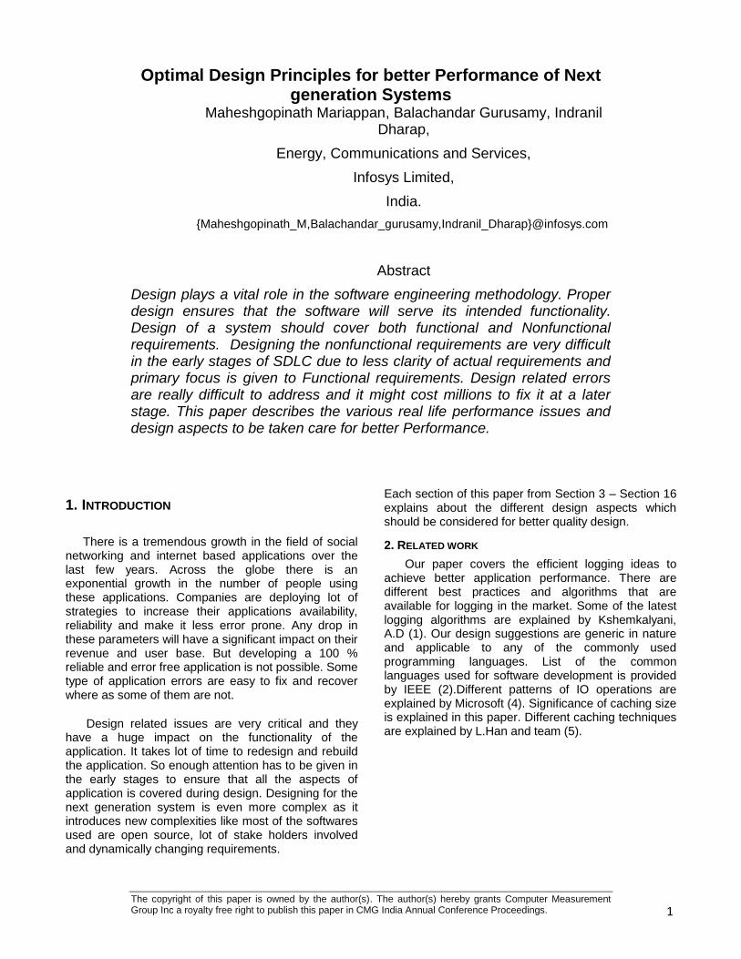
Traditionally logging was considered as a way to store all the info related to the application request and response. This info was used by the operations and dev teams during debugging of the application. Over a period of time there is a major shift in this trend. Now a day’s business mainly relies on this data to generate business metrics and reports. They also use the log data to identify the Usage pattern and Customer churn. Advancement of research in the areas of Cloud computing and big data as well as availability of efficient tools like Splunk made this analysis possible. So there is a push and urge from different stake holders of the products like sales, business and care to log as much info as possible related to the user request. The following are the common problems faced because of poor logging design

1. Slow response time

2. Application performance degradation

Case study:

A real time web application was hanging after running in the production environment for 5 hrs. After analysis we were able to identify the root cause of the issue. That application was logging the entire request, response with headers and all the Meta into log files. After filtering out the unnecessary logging, the system was able to run without any issues. Extra measures needs to be taken incase if system is asynchronous in nature (Node.js) and single threaded. We should not lock the master process in logging. If the main thread is get locked than all the requests into the system file up until the main thread is released and available.

Aspects that needs to be considered during the design are

1. Proper logging level

2. Log only the critical details of the session like, session id, user id, type of operation performed etc., instead of logging all the details

3. Storing logs to a file system or local system instead of trying to write across the network

4. Set proper rollback size and policy for logging

5. Enable auto archival for logging

6. If possible make logging as async process

Relationship between improvement of throughput and logging level is explained in this picture

Figure1: Logsize vs Throughput,Response Time

4. Programming language:

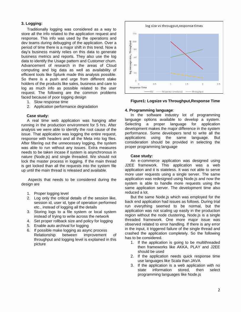
In the software industry lot of programming language options available to develop a system. Selecting a proper language for application development makes the major difference in the system performance. Some developers tend to write all the applications using the same language. But consideration should be provided in selecting the proper programming language

Case study:

An e-commerce application was designed using J2EE framework. This application was a web application and it is stateless. It was not able to serve more user requests using a single server. The same application was redesigned using Node.js and now the system is able to handle more requests using the same application server. The development time also reduced a lot.

But the same Node.js which was employed for the back end application had issues as follows. During trial run everything seemed to be normal, but the application was not scaling up easily in the production region without the node clustering, Node.js is a single threaded framework. One more major issue was observed related to error handling. If there is any error in the input, it triggered failure of the single thread and crashed the application completely. So the following has to be considered.

1. If the application is going to be multithreaded then frameworks like AKKA, PLAY and J2EE should be used

2. If the application needs quick response time use languages like Scala than JAVA

3. If the application is a web application with no state information stored, then select programming languages like Node.js

3

Figure2:Responsetime vs Programming launguage

3.3 Reducing IO calls:

IO related calls like DB and File operations are generally costly. These should be limited as much as possible.

Case study:

A mobile back end application’s goal was to collect the user preference, debug logs from mobile clients and store it in the DB. During the initial testing everything seemed to be fine. But during the production launch the response time was increased drastically. We did an analysis and observed that the client was calling multiple times DB to store and retrieve the user preference and logs. So caching solution was added in between client and DB layer to provide most frequently requested data

1. Employ a caching mechanism

2. Group the DB write calls

3. Using the Async driver if available

5. Selection of DB

Selection of appropriate DB is also a critical factor. Now a days there is a trend among technical community to go for No SQL DB for each and every application. But that is not the right approach. The following are common problems if the DB selection is not correct.

1. Query becomes very complex if the data stored is not in proper format.

2. Query takes more time to execute and compute results than the expected interval

3. Overall slow response to the end user

Case study:

An application was designed to store various trouble tickets and their status. Development team decided to develop this entire application with new softwares like NoSQL databases. But during the POC it was observed that RDBMS are better than NoSQL for relational, transaction based system.

The best design practices for the selection of Database are

1. Use Relational DB’s such as SQL, if there is relation among the data getting stored and system needs frequent reads

2. NoSQL DB’s are useful for storing voluminous data without relation and with more writes and less reads

6. Replication strategies:

Applications are deployed across different data centers and clusters. In this case sometimes data replication is required across the servers to serve the users without any functional glitch. There are two strategies followed for data replication

1. Synchronous data replication

2. Asynchronous data replication.

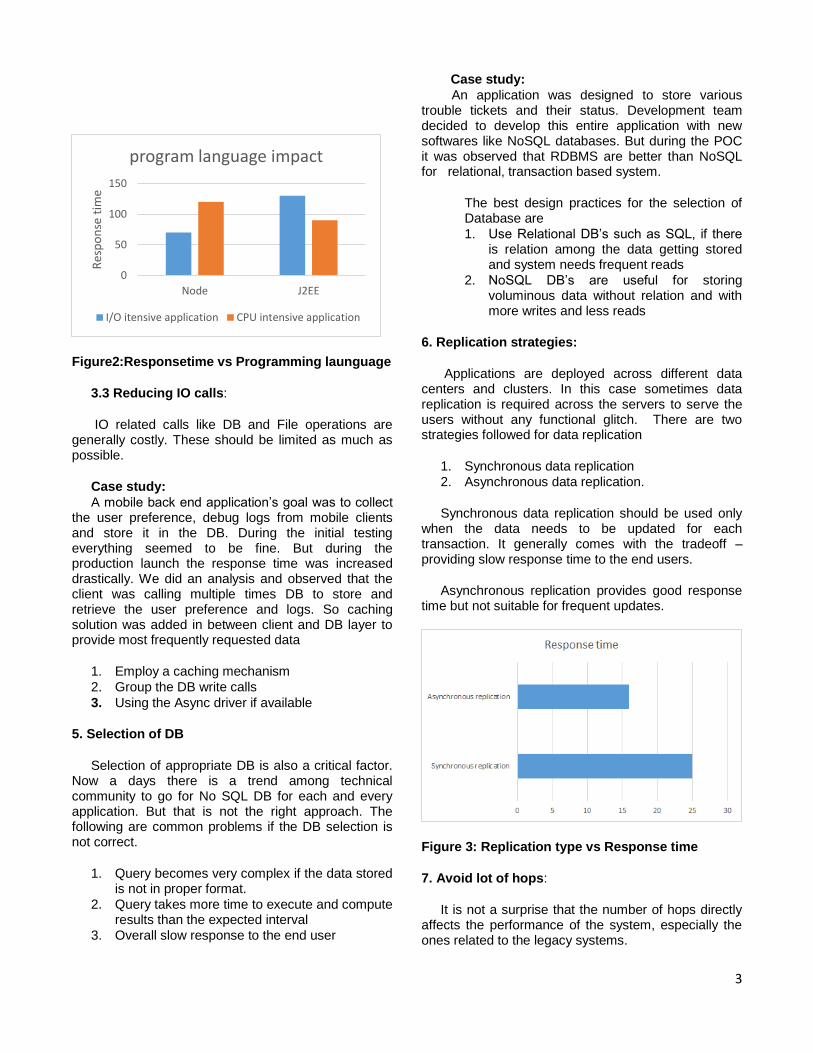
Synchronous data replication should be used only when the data needs to be updated for each transaction. It generally comes with the tradeoff –providing slow response time to the end users.

Asynchronous replication provides good response time but not suitable for frequent updates.

Figure 3: Replication type vs Response time

7. Avoid lot of hops:

It is not a surprise that the number of hops directly affects the performance of the system, especially the ones related to the legacy systems.

0

50

100

150

Node J2EE

Res

po

nse

tim

e

program language impact

I/O itensive application CPU intensive application

4

Case study:

When a provisioning engine was deployed in Production it took more than an hour to provision a single user account. Lot of analysis was done to identify the root cause of the problem. The system was sourcing from more than 50 legacy services to fetch the info and creating the user entry during provisioning. Each system took some milliseconds to process the request. During further analyzes it was observed that all these legacy systems were built on top of the original source of truth and each one of them adding some extra small functions which is not required for the provisioning engine.

After a series of discussions with all our stake holders we retired the unwanted systems and rewrote the original source of truth in such a way that it provides all the required data directly. The response time then improved a lot from an hour to less than 10 sec. So always remember to avoid the unnecessary hops in larger systems.

Figure 4 : Number of hops vs Response time

8. Caching:

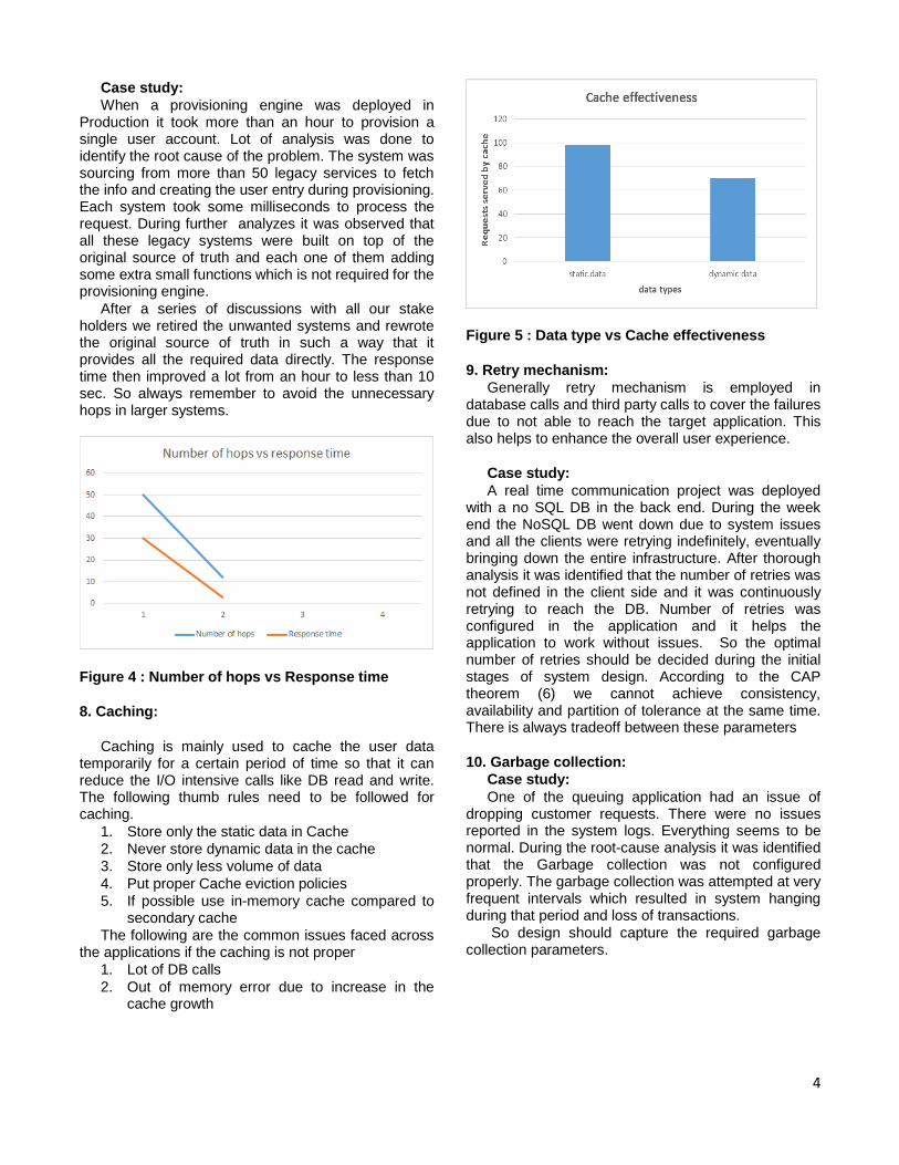
Caching is mainly used to cache the user data temporarily for a certain period of time so that it can reduce the I/O intensive calls like DB read and write. The following thumb rules need to be followed for caching.

1. Store only the static data in Cache

2. Never store dynamic data in the cache

3. Store only less volume of data

4. Put proper Cache eviction policies

5. If possible use in-memory cache compared to secondary cache

The following are the common issues faced across the applications if the caching is not proper

1. Lot of DB calls

2. Out of memory error due to increase in the cache growth

Figure 5 : Data type vs Cache effectiveness

9. Retry mechanism:

Generally retry mechanism is employed in database calls and third party calls to cover the failures due to not able to reach the target application. This also helps to enhance the overall user experience.

Case study:

A real time communication project was deployed with a no SQL DB in the back end. During the week end the NoSQL DB went down due to system issues and all the clients were retrying indefinitely, eventually bringing down the entire infrastructure. After thorough analysis it was identified that the number of retries was not defined in the client side and it was continuously retrying to reach the DB. Number of retries was configured in the application and it helps the application to work without issues. So the optimal number of retries should be decided during the initial stages of system design. According to the CAP theorem (6) we cannot achieve consistency, availability and partition of tolerance at the same time. There is always tradeoff between these parameters

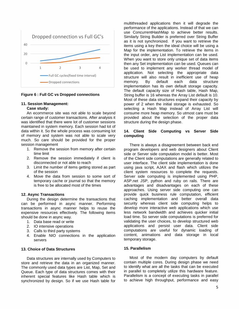
10. Garbage collection:

Case study:

One of the queuing application had an issue of dropping customer requests. There were no issues reported in the system logs. Everything seems to be normal. During the root-cause analysis it was identified that the Garbage collection was not configured properly. The garbage collection was attempted at very frequent intervals which resulted in system hanging during that period and loss of transactions.

So design should capture the required garbage collection parameters.

5

Figure 6 : Full GC vs Dropped connections

11. Session Management:

Case study:

An ecommerce site was not able to scale beyond certain range of customer transactions. After analysis it was identified that there were lot of customer sessions maintained in system memory. Each session had lot of data within it. So the whole process was consuming lot of memory and system was not able to scale very much. So care should be provided for the proper session management

1. Remove the session from memory after certain time limit

2. Remove the session immediately if client is disconnected or not able to reach

3. Limit the number of items getting stored as part of the session

4. Move the data from session to some sort of temporary cache or journal so that the memory is free to be allocated most of the times

12. Async Transactions

During the design determine the transactions that can be performed in async manner. Performing transactions in async manner helps to reuse the expensive resources effectively. The following items should be done in async way.

1. Data base read or write

2. IO intensive operations

3. Calls to third party systems

4. Enable NIO connections in the application servers

13. Choice of Data Structures

Data structures are internally used by Computers to store and retrieve the data in an organized manner. The commonly used data types are List, Map, Set and Queue. Each type of data structures comes with their inherent special features like Hash table which is synchronized by design. So if we use Hash table for

multithreaded applications then it will degrade the performance of the applications. Instead of that we can use ConcurrentHashMap to achieve better results. Similarly String Builder is preferred over String Buffer as it is not synchronized. If you want to retrieve the items using a key then the ideal choice will be using a Map for the implementation. To retrieve the items in the input order, any List implementation can be used. When you want to store only unique set of data items then any Set implementation can be used. Queues can be used to implement any worker thread model of application. Not selecting the appropriate data structure will also result in inefficient use of heap memory. By default each data structure implementation has its own default storage capacity. The default capacity size of Hash table, Hash Map, String buffer is 16 whereas the Array List default is 10. Most of these data structures expand their capacity by power of 2 when the initial storage is exhausted. So selecting a Hash Map instead of Array List will consume more heap memory. So utmost care must be provided about the selection of the proper data structure during the design phase.

14. Client Side Computing vs Server Side computing

There is always a disagreement between back end program developers and web designers about Client side or Server side computation model is better. Most of the Client side computations are generally related to user interface. The client side implementation is done using java script, AJAX and flash which utilizes the client system resources to complete the requests. Server side computing is implemented using PHP, ASP.net JSP, python and ruby on rails. There are advantages and disadvantages on each of these approaches. Using server side computing one can provide quick business rule computation, efficient caching implementation and better overall data security whereas client side computing helps to develop more interactive web applications which use less network bandwidth and achieves quicker initial load time. So server side computations is preferred for validating the user choices, to develop structured web applications and persist user data. Client side computations are useful for dynamic loading of content, animations and data storage in local temporary storage.

15. Parallelism

Most of the modern day computers by default contain multiple cores. During design phase we need to identify what are all the tasks that can be executed in parallel to completely utilize this hardware feature. Parallelism is a concept of executing tasks in parallel to achieve high throughput, performance and easy

0

20

40

1 2 3 4

Dropped connection vs Full GC's

Full GC cycles(fixed time interval)

Dropped connections

6

scalability. To achieve parallelism in the application we need to identify the set of tasks that can be executed independently without waiting for others. Large work/transaction should be broken into small work units/tasks. Dependency between these work units and communication overhead between these units should be identified during the design phase. Then work units can be assigned to the central command unit for execution. Finally the results should be combined and sent to the user. One good example of this design is MapReduce programming technique. According to design rule hierarchies paper (7) Software modules located within the same layer of the hierarchy, suggest independent, hence parallelizable, tasks. Dependencies between layers or within a module suggest the need for coordination during concurrent work. So use as much parallelism as possible during the design to achieve better performance.

16. Choice of Design patterns

Design patterns provides a solution approach to the commonly recurring problems in a particular context. Concepts of design pattern started with the initial set of patterns described by the gang of four in their design patterns book. Currently around 200 design patterns available to resolve different software problems. So the cumbersome task is identifying the suitable design pattern for the application. One of the good approach is to design pattern Intent ontology proposed by Kampffmeyer H., Zschaler S in their paper (7).

They have also developed a tool to identify the suitable design pattern for the problem. Once a particular pattern is identified it has to be checked to ensure that it doesn’t belong to Anti patterns.

17. CONCLUSION:

As the next gen systems becomes more complex and pose a challenge on its own, it is imperative that while designing these systems, we follow the points discussed in this paper. Based on our experience over the years, a system proves to be efficient and cost-effective only when more weightage is given and adequate time is spent in designing the system. Brief design topics are

1. Proper logging configuration

2. Appropriate selection of software language

3. Reduce number IO operations

4. Appropriate selection of databases

5. Suitable replication strategy

6. Retire/merge unwanted legacy systems

7. Implement proper caching mechanism

8. Proper retry interval at client side

9. Proper garbage collection configuration

10. Keep less data in session memory

11. Priority to Async transaction

12. Proper choice of data structure.

13. Client Side computing vs Server Side computing

14. Parallelism

15. Choice of Design patterns

Each one of the above mentioned design principle will surely help in achieving better performance and good customer experience.

18. REFERENCES:

1. A. Kshemkalyani "A Symmetric O(n log n) Message Distributed Algorithm for Large-Scale Systems", Proc. IEEE Int\'l Cluster Computing Conf., 2009

2. http://spectrum.ieee.org/at-work/tech-careers/the-top-10-programming-languages

3. N. Ali, P. Carns, K. Iskra, D. Kimpe, S. Lang, R. Latham, R. Ross, L. Ward, and P. Sadayappan. Scalable I/O forwarding framework for high-performance computing systems. In IEEE International Conference on Cluster Computing (Cluster 2009), New Orleans, LA, September 2009.

4. http://msdn.microsoft.com/en-us/library/windows/desktop/aa365683(v=vs.85).aspx

5. L. Han, M. Punceva, B. Nath, S. Muthukrishnan, and L. Iftode, "SocialCDN: Caching techniques for distributed social networks, " in Proceedings of the 12th IEEE International Conference on Peer-to-Peer Computing (P2P), 2012.

6. http://en.wikipedia.org/wiki/CAP_theorem.

7. Sunny Wong, Yuanfang Cai, Giuseppe Valetto, Georgi Simeonov, and Kanwarpreet Sethi”Design Rule Hierarchies and Parallelism in Software Development Task”

8. Kampffmeyer H., Zschaler S., “Finding the Pattern You Need: The Design Pattern Intent Ontology”, in MoDELS, Springer, 2007, volume 4735, pages 211-225

The copyright of this paper is owned by the author(s). The author(s) hereby grants Computer Measurement Group Inc a royalty free right to publish this paper in CMG India Annual Conference Proceedings. 7

ARCHITECTURE AND DESIGN FOR PERFORMANCE OF A LARGE EUROPEAN BANK PAYMENT SYSTEM

Nityan Gulati Principal Consultant Tata Consultancy Services Ltd

Nityan.gulati@tcs.com Gurgaon

R. Hari Kumar

Senior Consultant Tata Consultancy Services

r.harikumar@tcs.com Bangalore

A Large software system is typically characterized by a large volume of transactions to be processed, considerable infrastructure and high number of concurrent users. Additionally it usually involves integration with a large number of up-stream and down-stream interfacing systems with varying processing requirements and constraints. The above parameters on its own may not pose a challenge when they are static in nature, but it gets tricky if the inputs keep changing and continuously evolving. In such conditions, how do we keep the system performance and resilience under control? This paper tries to explain the key design aspects that will need to be considered across various architectural layers to ensure a smooth post production performance.

1. INTRODUCTION

In a typical implementation, often due attention is not paid to the system performance during the initial stages of design and development. Performance testing happens at a later stage; sometimes just a few weeks before the application goes live As a result, only a very limited performance tuning options are available at this stage. We can do a bit of SQL tuning and some tweaking in the system configuration. Due to a lack of systematic and timely approach to address the performance issues, mostly these steps result in little gains.

While a large system involves several design aspects, we shall discuss some key application design areas and guidelines that need to be borne in mind during the design stage for robust and performing implementations.

Specifically, the paper illustrates key aspects to be considered in tuning web page response time, aspects in tuning straight through processing (STP) throughput, factors for improving the batch throughput and a number of other parameters to be considered for tuning.

The document is based on the experiences from tuning the architecture, design and code of several product based implementations of financial applications.

The examples and statistics quoted are derived from the actual experience from managing the design and architecture of payment platform for a large European Bank.

The system has gone live successfully and is in production for around two years now.

The paper is organized as follows:

Section 2 provides the context of the payment system, SLA requirements and a brief overview on the architecture of the system, Section 3 provides the key design considerations and parameters that are discussed in the paper, Section 5 to 7 discusses in detail the tuning activity that was done on the selected parameters, Section 8

8

summarizes the key performance benefits realized after the various parameters were tuned and finally section 9 enumerates the key lessons learnt from the project followed by references

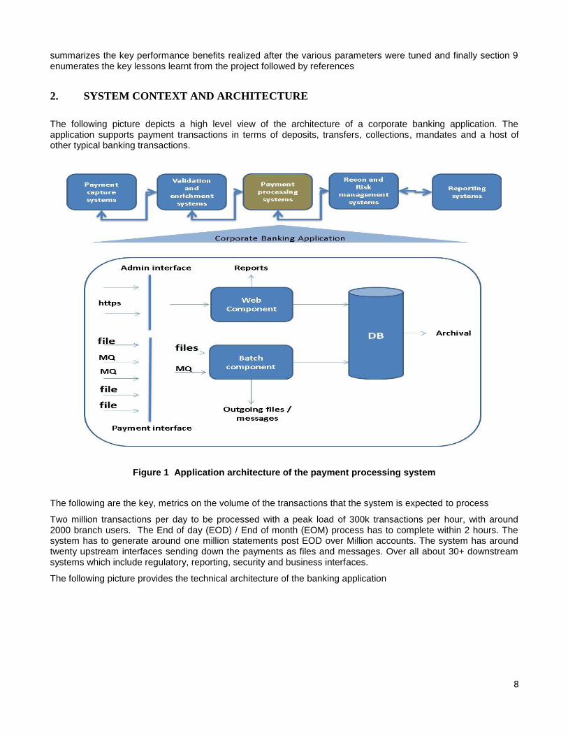
2. SYSTEM CONTEXT AND ARCHITECTURE

The following picture depicts a high level view of the architecture of a corporate banking application. The application supports payment transactions in terms of deposits, transfers, collections, mandates and a host of other typical banking transactions.

Figure 1 Application architecture of the payment processing system

The following are the key, metrics on the volume of the transactions that the system is expected to process

Two million transactions per day to be processed with a peak load of 300k transactions per hour, with around 2000 branch users. The End of day (EOD) / End of month (EOM) process has to complete within 2 hours. The system has to generate around one million statements post EOD over Million accounts. The system has around twenty upstream interfaces sending down the payments as files and messages. Over all about 30+ downstream systems which include regulatory, reporting, security and business interfaces.

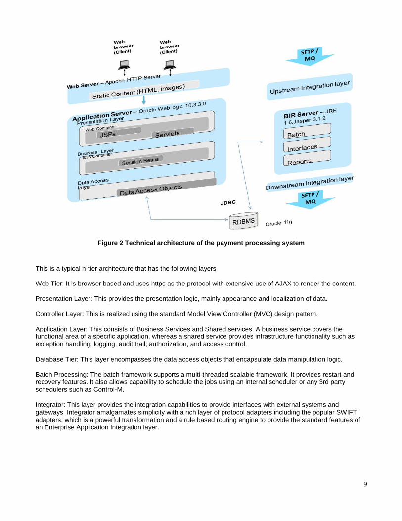
The following picture provides the technical architecture of the banking application

9

Figure 2 Technical architecture of the payment processing system

This is a typical n-tier architecture that has the following layers

Web Tier: It is browser based and uses https as the protocol with extensive use of AJAX to render the content. Presentation Layer: This provides the presentation logic, mainly appearance and localization of data. Controller Layer: This is realized using the standard Model View Controller (MVC) design pattern.

Application Layer: This consists of Business Services and Shared services. A business service covers the functional area of a specific application, whereas a shared service provides infrastructure functionality such as exception handling, logging, audit trail, authorization, and access control.

Database Tier: This layer encompasses the data access objects that encapsulate data manipulation logic. Batch Processing: The batch framework supports a multi-threaded scalable framework. It provides restart and recovery features. It also allows capability to schedule the jobs using an internal scheduler or any 3rd party schedulers such as Control-M.

Integrator: This layer provides the integration capabilities to provide interfaces with external systems and gateways. Integrator amalgamates simplicity with a rich layer of protocol adapters including the popular SWIFT adapters, which is a powerful transformation and a rule based routing engine to provide the standard features of an Enterprise Application Integration layer.

10

3. DESIGN CONSIDERATIONS

This section covers the key challenges that we faced in the various architectural layers of the system and the thought process adopted for resolution.

The following are the challenges that are discussed in this paper

3.1 Tuning web page parameters Performance of search screens considering the variety of search options and parameters available to the user and huge transaction volumes that are added to the system on a daily basis. Search capability is fundamental to the daily usage of the business users to carry out their daily tasks. The SLA mandated by the customer is to have a screen response of 2 seconds or less

3.2 Tuning STP throughput parameter (Straight through processing) Design for maintaining the STP throughput considering the following parameters

Number (Count) of payment files received from the upstream systems at any given point in time and non-uniformity in the size of the files received. The files could be single transaction file or bulk set of transaction files.

The SLA is to process a load of 300,000 transactions received as messages, files (single and bulk) of varying sizes under 60 minutes.

3.3 Tuning batch parameters The performance of batch programs largely depends on effective management of database contentions and optimal commit sizes. Considering the fact that we could receive more than 40% of the transactions from a single account, it could result in hot spots. The batch process can be quite intensive pumping up a large number of transactions. We had to tune the system where the commit rates were in excess of 10,000 per second.

The SLA is to complete the End of day batch profile (EOD) and the End of the month batch profile less than 2 hours. The peak volume of a business day was about two million transactions. Additionally, the following parameter tunings are considered

Database parameters tuning.

Oracle specific considerations.

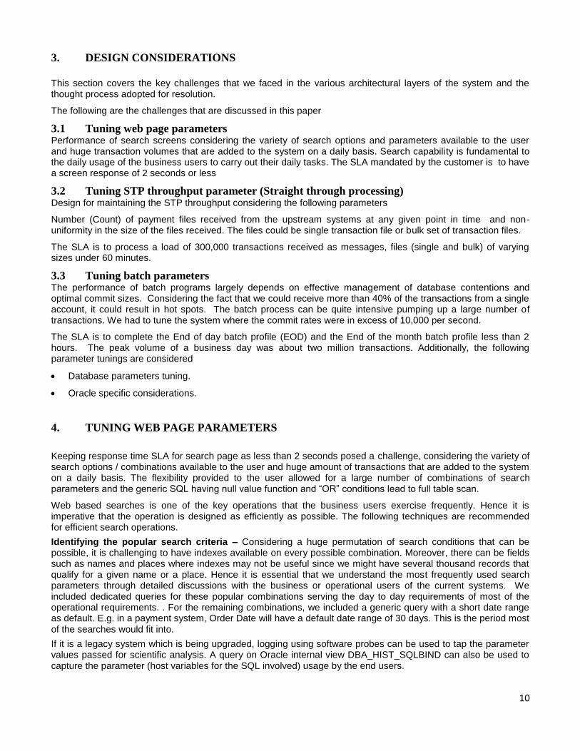
4. TUNING WEB PAGE PARAMETERS

Keeping response time SLA for search page as less than 2 seconds posed a challenge, considering the variety of search options / combinations available to the user and huge amount of transactions that are added to the system on a daily basis. The flexibility provided to the user allowed for a large number of combinations of search parameters and the generic SQL having null value function and “OR” conditions lead to full table scan.

Web based searches is one of the key operations that the business users exercise frequently. Hence it is imperative that the operation is designed as efficiently as possible. The following techniques are recommended for efficient search operations.

Identifying the popular search criteria – Considering a huge permutation of search conditions that can be possible, it is challenging to have indexes available on every possible combination. Moreover, there can be fields such as names and places where indexes may not be useful since we might have several thousand records that qualify for a given name or a place. Hence it is essential that we understand the most frequently used search parameters through detailed discussions with the business or operational users of the current systems. We included dedicated queries for these popular combinations serving the day to day requirements of most of the operational requirements. . For the remaining combinations, we included a generic query with a short date range as default. E.g. in a payment system, Order Date will have a default date range of 30 days. This is the period most of the searches would fit into.

If it is a legacy system which is being upgraded, logging using software probes can be used to tap the parameter values passed for scientific analysis. A query on Oracle internal view DBA_HIST_SQLBIND can also be used to capture the parameter (host variables for the SQL involved) usage by the end users.

11

Gracefully stopping the long running SQLs - A long running online query in the database is not under the control of the Application Server. It can block the Application Server thread for considerable amount of time thus impacting concurrency. In Oracle RDBMS such a query, can be interrupted gracefully if we create a dedicated Oracle user id for usage in the Application Server data source. This user id is assigned an Oracle Profile which has a limit set for CPU_PER_CALL (units are 1/100 of CPU seconds). Whenever an SQL running under that user id exceeds the specified, an Oracle Error ORA 02393 is returned and the query is terminated. Application code will trap it and a meaningful message is sent to the end user

Tuning the blank Search - This is a special case of open ended Search where the end user does not pass any parameters at all. This means all data is part of the result set and as the data is invariably sorted, it means sorting millions of rows and then presenting the first few rows. The only way to address this is to guide the Query Plan (at times via HINTS) so that an index with column order matching the sort order is picked up to avoid the costly sort operation. Also, we decided to suppress this Open Search feature wherever it is not required.

Additionally we added a data filter which will restrict the size of the result set to a smaller set. This makes sense as a blank search would otherwise bring up multiple pages of data that is not really useful to the user.

4.1 Quick Tuning Steps that lead to further benefits

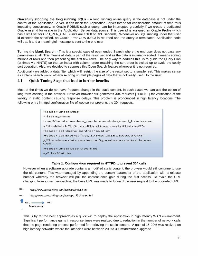
Most of the times we do not have frequent change in the static content. In such cases we can use the option of

long term caching in the browser. However browser still generates 304 requests [PERF001] for verification of the

validity in static content causing response delays. This problem is pronounced in high latency locations. The

following entry in httpd configuration file of web server prevents the 304 requests.

Table 1: Configuration required in HTTPD to prevent 304 calls

However when a software upgrade contains a modified static content, the browser would still continue to use

the old content. This was managed by appending the context parameter of the application with a release

number whereby the browser will pull the content once gain during the first access. To avoid the URL

changing from a user perspective, the base URL was made to forward the user request to the upgraded URL

This is by far the best approach as a quick win to deploy the application in high latency WAN environment.

Significant performance gains in response times were realized due to reduction in the number of network calls

that the page rendering process performed for retrieving the static content. A gain of 15-20% was realized on

high latency networks where the latencies were between 200 to 300msBrowser Upgrade

12

It has to be noted that IE 8 / IE9 give superior performance as compared to IE 7 on account of efficient

rendering APIs in these versions. The performance of the web pages improved 10 to 15% without requiring

any code changes.

5. STP THROUGPUT PARAMETER TUNING

Design for maintaining the STP throughput considers the following parameters:

Number of files received at any point of time and no uniformity in the size of the files received by the system. Random combinations of small, medium and large sized files are received from the upstream interfaces. A file considered small varies from ~1 to 100 KB based on the record length of the transaction. A medium file varies from 100 to 1000KB. A file is considered large when it is in excess of 1 MB. We were expected to receive files of size up to 60MB.

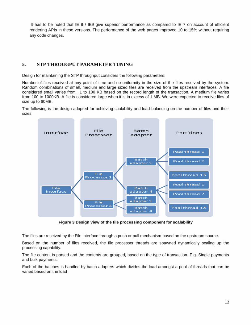
The following is the design adopted for achieving scalability and load balancing on the number of files and their sizes

Figure 3 Design view of the file processing component for scalability

The files are received by the File interface through a push or pull mechanism based on the upstream source.

Based on the number of files received, the file processer threads are spawned dynamically scaling up the processing capability.

The file content is parsed and the contents are grouped, based on the type of transaction. E.g. Single payments and bulk payments.

Each of the batches is handled by batch adapters which divides the load amongst a pool of threads that can be varied based on the load

13

6. TUNING BATCH PARAMETERS

Batch jobs are a standard way of processing the transactions at the end of the day for doing interest calculations, account management and other risk management jobs. The volume of the transactions at the end of the day can be quite high. In our case, the peak volume of transactions expected was about two million transactions.

The application software should be able to scale up and fully exploit the available resources viz. CPU, Memory etc. in a manner such that there is minimal contention amongst parallel paths of execution.

Multithreading support is provided by Java. The Batch frameworks should exploit the same. However; the various hotspots which cause concurrency issues degrade the gains from multi-threading.

The guidelines below were used to mitigate the contentions

Sequence Caching – Batch Processing needs a large number transaction IDs to be generated. Using oracle generated sequences enable them to be easily generated and assigned to the transactions. Caching them upfront reduces the overhead of ID generation and leads to improvement of performance of the batch processing. Oracle Sequences typically used in primary keys should be cached as much as possible (default is 20) if there is no business constraint. The NOORDER clause should be preferred. This technique improved the performance of the SQL performance of our application thereby improving the batch throughout considerably.

Allocation of Transactions to Threads - Allocation of transactions to the threads avoids situation, where transactions processed over multiple threads in parallel, can enter into contention (Oracle row lock contention wait). An example is the case - where transactions of the same account are getting processed in parallel across Threads and doing ‘Select for Update’ on the Account row. The contention can be reduced if the model is changed and the threads pick up the transactions based on the modulus of the Account Id. Modulus is a mathematical function that finds the remainder of division of one number by another. This technique helped us to route the transaction evenly across the threads thereby reducing the hot spots

Usage of Right Data Structures - Usage of better container collection classes promotes better concurrency. We adopted concurrent hash map which reduced the cases where the transactions were entering into dead lock situations.

Parallelism in batch profile - This can bring in much needed time reduction in the overall EOD cycle. We engaged the functional SMEs to redesign the EOD profile carefully so that non conflicting Batch programs can be run in parallel.

Deadlock Prevention- Deadlocks need to be avoided at by planning and proper design. For this, the updates should be at the end, just before the commit as far as possible. The Tables should be updated in a consistent order in all programs running in parallel e.g. Table A, followed by Table B followed by Table C. Details of deadlocks, the SQLs and rows involved can be seen in the Alert Log and Trace files generated by Oracle. The above technique helped us to reduce the deadlocks when files were received with several transactions on a small set of accounts.

7. TUNING DATABASE PARAMETERS

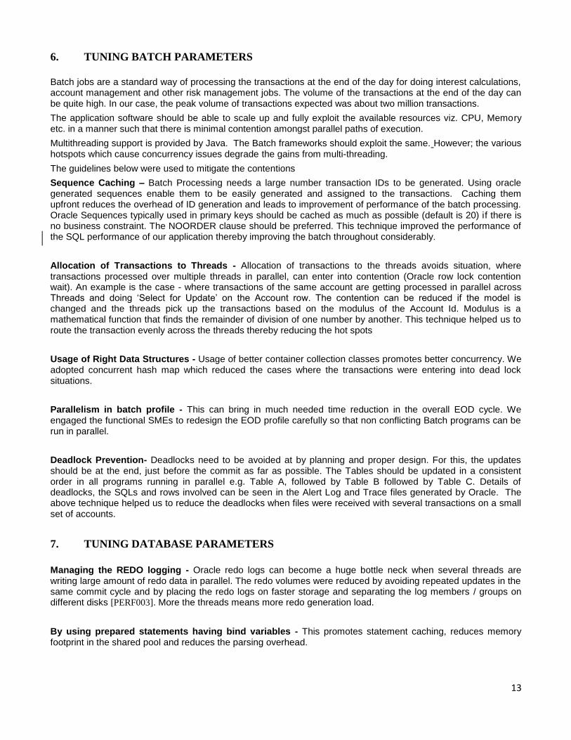
Managing the REDO logging - Oracle redo logs can become a huge bottle neck when several threads are writing large amount of redo data in parallel. The redo volumes were reduced by avoiding repeated updates in the same commit cycle and by placing the redo logs on faster storage and separating the log members / groups on different disks [PERF003]. More the threads means more redo generation load.

By using prepared statements having bind variables - This promotes statement caching, reduces memory footprint in the shared pool and reduces the parsing overhead.

14

Bulking of Inserts/Updates – Inserts/Updates were clubbed using the add Batch and execute Batch JDBC methods. This is highly useful in an IO bound application. It saves on network round trips and especially useful where latency between the application and database servers is high.

Disabling Auto Commit mode – As a default, the JDBC connection commits at every Insert/Update/Delete statement. This can not only lead to too many commits resulting in the infamous ‘log file sync wait’ [PERF002] but

can also lead to integrity problems as it breaks the atomic unit of work principle.

Ensuring closure of Prepared statement and Connection – This will conserve the JDBC resources and prevent database connection leakage. This is done in the ‘finally’ block in Java so that even in exceptions we close the resources before exiting.

Connection Pool libraries - This saves on JDBC connection count and promotes better management and control. Industry standard Application Servers use this as a standard practice. The same may now be used in the batch frameworks. In this context right configuration of pool is very important, especially the minimum/maximum pool sizes else the application threads will wait for the connections. “BoneCP” is a third party connection pool management library which was used in our application. It does a good job of managing the pool effectively.

Controlling the JDBC Fetch Size – The result set rows are retrieved from the database server in lots as per the JDBC fetch size. Based on this size the JDBC driver allocates memory structures in the Heap to accommodate the arriving data. Fetch size determines the number of chunks of row-sets that oracle return for a given query. The default value is 10. This will mean, oracle will return in 10 row-sets if the result set size is 100 rows. Too less a value will mean more network traffic between client and the database. Too high a value will impact the heap memory available on the client. The fetch size selected should be optimal to balance the network traffic and the available heap available on the client side. A large fetch size can lead to out of memory errors. Cases where the code tries to fetch data with same size of the rows to be shown on screens can result in out of memory issues. We selected a fetch size of 100, based on the maximum number of records that a user would normally want to view on a given search criteria

Database Clustering - Implementing Real application cluster can help scale the database layer largely. It is one of the most important layers at which an issue is normally cascaded across all the layers. RAC is a special case and unless application is designed for RAC, it is going to degrade 30% or more on account of RAC related waits related to transfer of Oracle data blocks over the high speed interconnect, across the SGAs of the different RAC nodes. While index hash partitioning, sequence caching etc. can give some relief, real improvement comes from right application work load partitioning in sync with database Table partitioning.

For example - in a two Entity scenario, JVMs processing Entity 1 connect to RAC node A as a preferred instance (using Oracle Services) and JVMs processing Entity 2 connect to RAC node B as a preferred instance. The required Tables are partitioned on Entity Id and the Partitions are mapped onto separate Table spaces to isolate the blocking scenarios. All this helps mitigate the RAC related damages and promotes improved performance, scalability and availability. It implies that at design stage enough thought has been given for RAC enablement.

Implementation of RAC in the program was postponed as there was no infrastructure support available in the client environment

Oracle specific considerations [PERF003]

Physical Design: The physical design of database storage has an important impact on overall performance of

the database

The following are the factors that were considered for optimizing the database design:

The physical arrangement of table spaces on storage volumes (hard disks) along with the mapping of database objects (tables, indexes, etc.) on to the table spaces.

The number of redo log groups, their member count, and log file sizes and placement. (E.g. log groups and their members to be placed on separate and very fast disks.)

15

The storage options of database objects within a table space (e.g. In Oracle, options to be set in the storage clause e.g. PCT free, extents should be exercised).

Definition of indexes - which tables columns should be indexed, and the type of index (e.g. B Tree, bit mapped index (recommended for status type columns etc.).

Other performance tuning options, depending on RDBMS features (e.g. partitioned tables, materialized views should be exploited)

Table Partitioning - If volumes are going to be high, table partitioning has to be thought in advance rather than later when we have performance issues. For databases above 1 TB, partitioning must be an essential consideration. It reduces the hot spots such as index last block, where we have sequentially increasing keys for the index. We considered both Table and Index Partitioning to get the best gains.

Partitioning helped us greatly in large scale removal of data during archival and purging process. For example

removal of Jan 2012 data from the database Table can be done very fast by dropping the monthly Partition as

compared to conventional delete of millions of rows. Additionally, it helped us to improve the maintenance of the

database e.g. Partitions were backed up independently; Partitions were marked ‘read only’ to save backup time.

8. KEY BENEFITS REALIZED

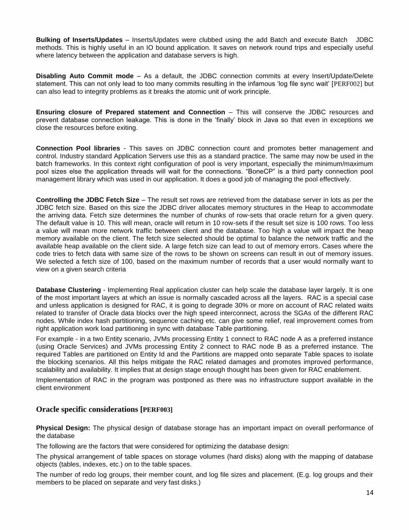
8.1 Web performance The design criteria adopted for web page performance helped us to manage the SLA expectation of the users. While the logged in users were expected to be around 2000 users, the concurrent usage was 200 users.

Figure 4 Average Response Time of the top 10 frequent use cases

X-axis >> Average response range, Y axis >> Actual graph value

16

The search page performance was manageable even when a portion of the users did fire blank searches. Queries were adjusted to include a shortened data range to manage the data volume.

The introduction of configuration in the web server to stop 304 calls originating from browser boosted the performance of the application in regions when the network latency was upwards of 200ms.

The graphical picture above shows the response times of key pages that the user community uses very frequently.

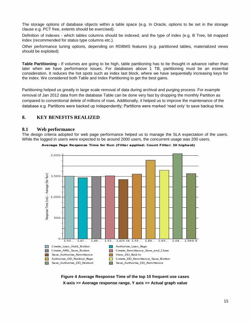
8.2 STP performance The design adopted for processing the files of varying sizes increased the throughput significantly. The dynamic spawning of file processors and splitting the huge files into manageable batches improved the scalability of the system dramatically.

The following matrix provides the split up of various files and messages totaling to 300,000 transactions per hour that the system was able to process in 60 minutes

Table 2: STP volumes to be supported on each of the key interfaces

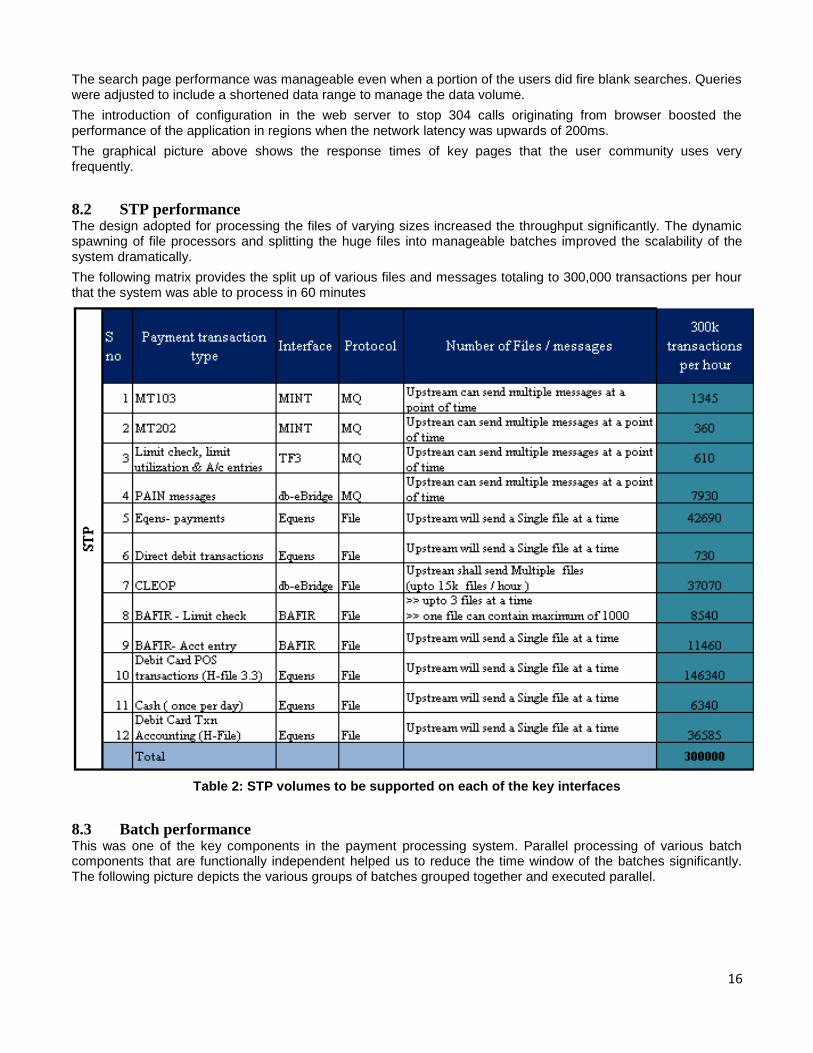
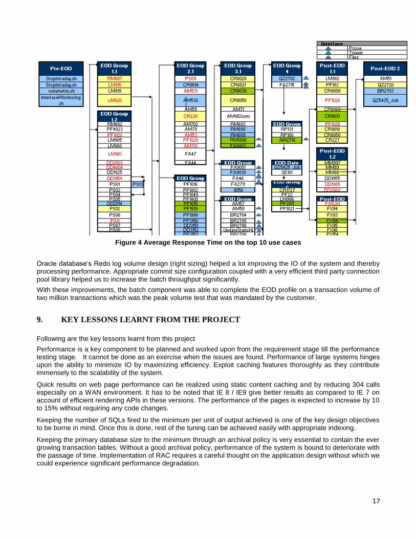
8.3 Batch performance This was one of the key components in the payment processing system. Parallel processing of various batch components that are functionally independent helped us to reduce the time window of the batches significantly. The following picture depicts the various groups of batches grouped together and executed parallel.

17

Figure 4 Average Response Time on the top 10 use cases

Oracle database‘s Redo log volume design (right sizing) helped a lot improving the IO of the system and thereby processing performance. Appropriate commit size configuration coupled with a very efficient third party connection pool library helped us to increase the batch throughput significantly.

With these improvements, the batch component was able to complete the EOD profile on a transaction volume of two million transactions which was the peak volume test that was mandated by the customer.

9. KEY LESSONS LEARNT FROM THE PROJECT

Following are the key lessons learnt from this project

Performance is a key component to be planned and worked upon from the requirement stage till the performance testing stage. It cannot be done as an exercise when the issues are found. Performance of large systems hinges upon the ability to minimize IO by maximizing efficiency. Exploit caching features thoroughly as they contribute immensely to the scalability of the system.

Quick results on web page performance can be realized using static content caching and by reducing 304 calls especially on a WAN environment. It has to be noted that IE 8 / IE9 give better results as compared to IE 7 on account of efficient rendering APIs in these versions. The performance of the pages is expected to increase by 10 to 15% without requiring any code changes.

Keeping the number of SQLs fired to the minimum per unit of output achieved is one of the key design objectives to be borne in mind. Once this is done, rest of the tuning can be achieved easily with appropriate indexing.

Keeping the primary database size to the minimum through an archival policy is very essential to contain the ever growing transaction tables. Without a good archival policy, performance of the system is bound to deteriorate with the passage of time. Implementation of RAC requires a careful thought on the application design without which we could experience significant performance degradation.

18

REFERENCES

[PERF001] Best practices for speeding up your web site. Yahoo developer network.

[PERF002] Oracle Tuning: The Definitive Reference: By Donald Burleson.

[PERF003] Oracle® Database Performance Tuning Guide.

The copyright of this paper is owned by the author(s). The author(s) hereby grants Computer Measurement Group Inc a royalty free right to publish this paper in CMG India Annual Conference Proceedings.

19

Designing for Performance Management of Mission Critical Software Systems in Production

Raghu Ramakrishnan TCS

A61-A, Sector 63 Noida, Uttar Pradesh, India

201301 91-9810607820

ramakrishnan.raghu@tcs.com raghuramakrishnan71@gmail.com

Arvinder Kaur USICT, GGSIPU

Sector 16C Dwarka, Delhi, India

110078 91-9810434395

arvinder70@gmail.com

Gopal Sharma TCS

A61-A, Sector 63 Noida, Uttar Pradesh, India

201301 91-9958444833

gopal1.sharma@tcs.com gopalsharma1972@gmail.com

Traditionally, the performance management of software systems in production has been a reactive exercise, often carried out after a performance bottleneck has surfaced or a severe disruption of service has occurred. In many such scenarios, the reason behind such behavior is never correctly identified primarily due to the absence of accurate information. The absence of historical records related to system performance also limits development of models and baselines for proactive identification of trends which indicate degradation. This paper seeks to change the way the performance management is carried out. It identifies five best practices that have been classified as requirements to be included as part of software system design and construction to improve the overall quality of performance management of these systems in production. These practices were successfully implemented in a mission critical software system at design time resulting in effective and efficient performance management of this system from the time it was operationalized.

1 Introduction The business and technology landscape of today is characterized by the increasing presence of mission critical web applications. These web applications have progressed from being simple static content providing applications to application allowing all kinds of business transactions. The responsiveness of websites under concurrent load of a large number of users is an important performance indicator for the end users and the underlying business. The growing focus on high performance and resilience has necessitated including comprehensive performance management as an integral part of the software systems. However this is an area which has received limited focus and relies on a fix-it-later approach from a project execution perspective. The key to the successful performance management of critical systems in production is timely availability and accuracy of data which may then be analyzed for proactive identification of performance incidents. The inclusion of performance management requirements is essential in the design and construction phase of a software system. Our experience in handling of performance related incidents in critical web application over the last few years has shown that the focus on inclusion of such techniques starts when performance incidents get reported after the start of operations of the software system in production. This may be too late since there may be little room left for any significant design change at that point of time or may require a major rework in the application. This approach

20

is risk prone and expensive as making changes in implementation phase of software development lifecycle is difficult, incurs rework effort and a 100 times increase in cost [YOGE2009]. A number of studies have shown that responsive websites impact productivity, profits and brand image of an organization in a positive manner. In addition, slow websites result in loss of brand value due to negative publicity and decreased productivity. A survey done by Aberdeen Group on 160 organizations reported an impact of up to 16% in customer satisfaction and 7% in conversions i.e. loss of a potential customer due to a one second delay in response time. The survey also reported that the best in class organizations improved their average application response time by 273 percent [SIMI2008]. Satoshi Iwata et al. demonstrates the usage of statistical process control charts based on median statistic for detecting performance anomalies related to processing time in RuBiS which is a web based prototype of an auction site [SATO2010]. This performance anomaly detection technique requires the timely availability of measured value using appropriate instrumentation techniques (e.g. response time from the web application). This paper tries to bring about a paradigm shift from the prevalent reactive and silo-based approach in the domain of performance monitoring of mission critical software systems to an analytics based engineering approach by including certain proven requirements as part of the design and design process. The objective is to be able to know about a performance issue before a complaint is received from the end users. The silo-based approach analyzes several dimensions such as web applications, web servers, application servers, database servers, storage, servers and network components in isolation. The reactive approach involves including logs in a makeshift manner only when a performance incident occurs. This in turn results in the required information not being available at the right time for effective detection, root cause analysis and resolution of the problem. This paper suggests including practices like instrumentation, system performance archive, controlled monitoring, simulation and an integrated operational console as part of the design and design process of software systems. These requirements are not aimed at improving or optimizing the performance of the software system but are for enhancing the effectiveness and efficiency of performance monitoring in production. These requirements were successfully included as part of the design and design process in a mission critical e-government domain web application built using J2EE technology. This has helped the production support team to recognize early warning signs which may lead to a possible performance incident and take corrective actions quickly. The rest of this paper is organized as follows. Section 2 describes the application in which the proposed best practices were implemented. Section 3 describes the best practices in detail. Section 4 presents the results and findings of our work. Section 5 provides the summary, conclusion, limitations of our work and suggestions for future work.

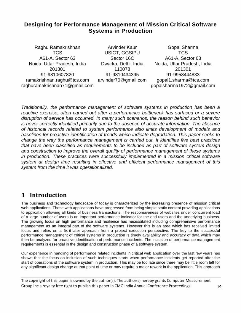
2 Background These requirements were successfully included as part of the design and design process in a mission critical e-government domain web application built using J2EE technology servicing more than 40000 customers every day. The web application in this e-governance program is used by both external and department users for carrying out business transactions. The external users access this application on the Internet and the department users access it on the Intranet. The technical architecture has five tiers for the external users and three tiers for the department users. The presentation components are JSPs and the business logic components are POJOs developed using the Spring framework. External Users: The information flow from external users passes through five tiers. The tiers 1, 2A and 3 host the web application server. The tiers 2B and 4 host the database server. Tier 1 provides the presentation services. Tier 2A and 2B carry out the request routing from the tier 1 to tier 3 after carrying out the necessary authentication and authorization checks. The business logic is deployed in tier 3. Tier 4 holds all transactional and master data of the application. Department Users: The information flow from department users passes through three tiers. The tier 5 and 6 host the web application server. Tier 5 provides the presentation tier. The business logic id deployed in Tier 6. Tier 4 holds all transactional and master data of the application.

21

Figure 2 shows the logical architecture of the e-government domain web application.

Figure 2: Logical architecture of the e-governance web application

3 Building Performance Management in Software Systems The existing approach of performance management of software systems in production involves a reactive and silo based approach. The silo based approach involves measurements at the IT infrastructure component level i.e. server, storage, web servers, application servers, database servers, network components and application server garbage collection health. The reactive approach involves adding log entries whenever a performance incident occurs. This section describes in detail five mandatory requirements that a software system needs to incorporate as part of the design and design process to ensure effective, proactive and holistic performance management after the system is in production. These requirements were successfully implemented as part of the design and design of a mission critical e-government domain web application with excellent results. This web application provides a number of critical business transactions to end users and requires meeting stringent performance and available service level agreement requirements.

3.1 Instrumentation

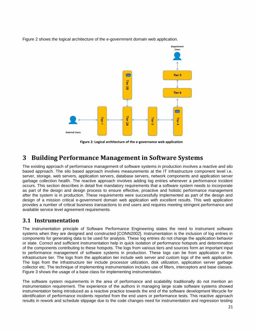
The instrumentation principle of Software Performance Engineering states the need to instrument software systems when they are designed and constructed [CONN2002]. Instrumentation is the inclusion of log entries in components for generating data to be used for analysis. These log entries do not change the application behavior or state. Correct and sufficient instrumentation help in quick isolation of performance hotspots and determination of the components contributing to these hotspots. The logs from various tiers and sources form an important input to performance management of software systems in production. These logs can be from application or the infrastructure tier. The logs from the application tier include web server and custom logs of the web application. The logs from the infrastructure tier include processor utilization, disk utilization, application server garbage collector etc. The technique of implementing instrumentation includes use of filters, interceptors and base classes. Figure 3 shows the usage of a base class for implementing instrumentation. The software system requirements in the area of performance and scalability traditionally do not mention an instrumentation requirement. The experience of the authors in managing large scale software systems showed instrumentation being introduced as a reactive practice towards the end of the software development lifecycle for identification of performance incidents reported from the end users or performance tests. This reactive approach results in rework and schedule slippage due to the code changes need for instrumentation and regression testing

22

required following these changes. This paper recommends inclusion of this practice as a key requirement in the software requirements specification rather than being limited to being a best practice.

PRACTICE: Include sufficient instrumentation in all tiers for quick isolation of performance

problems and identification of the component(s) contributing to performance problems.

public class TestBaseAction extends ActionSupport implements PrincipalAware, ServletRequestAware, SessionAware {

public final String execute() throws Exception {

String res; Date begin = new Date( ); res = execute2( ); Date end = new Date( );

logger.info(….end.getTime( ) – begin.getTime( ) ….);

}

} Figure 3: A base class is a place to add instrumentation log entries.

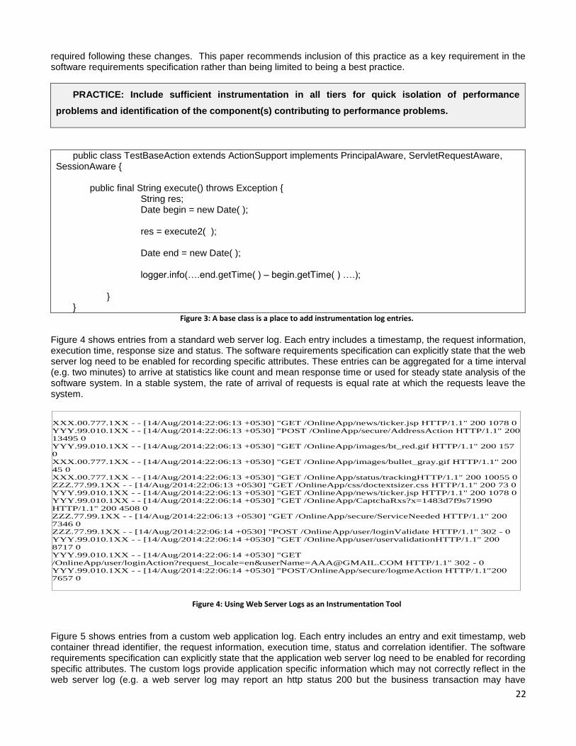
Figure 4 shows entries from a standard web server log. Each entry includes a timestamp, the request information, execution time, response size and status. The software requirements specification can explicitly state that the web server log need to be enabled for recording specific attributes. These entries can be aggregated for a time interval (e.g. two minutes) to arrive at statistics like count and mean response time or used for steady state analysis of the software system. In a stable system, the rate of arrival of requests is equal rate at which the requests leave the system.

Figure 4: Using Web Server Logs as an Instrumentation Tool

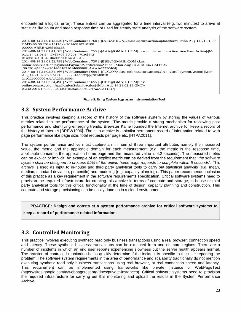
Figure 5 shows entries from a custom web application log. Each entry includes an entry and exit timestamp, web container thread identifier, the request information, execution time, status and correlation identifier. The software requirements specification can explicitly state that the application web server log need to be enabled for recording specific attributes. The custom logs provide application specific information which may not correctly reflect in the web server log (e.g. a web server log may report an http status 200 but the business transaction may have

XXX.00.777.1XX - - [14/Aug/2014:22:06:13 +0530] "GET /OnlineApp/news/ticker.jsp HTTP/1.1" 200 1078 0

YYY.99.010.1XX - - [14/Aug/2014:22:06:13 +0530] "POST /OnlineApp/secure/AddressAction HTTP/1.1" 200

13495 0

YYY.99.010.1XX - - [14/Aug/2014:22:06:13 +0530] "GET /OnlineApp/images/bt_red.gif HTTP/1.1" 200 157

0

XXX.00.777.1XX - - [14/Aug/2014:22:06:13 +0530] "GET /OnlineApp/images/bullet_gray.gif HTTP/1.1" 200

45 0

XXX.00.777.1XX - - [14/Aug/2014:22:06:13 +0530] "GET /OnlineApp/status/trackingHTTP/1.1" 200 10055 0

ZZZ.77.99.1XX - - [14/Aug/2014:22:06:13 +0530] "GET /OnlineApp/css/doctextsizer.css HTTP/1.1" 200 73 0

YYY.99.010.1XX - - [14/Aug/2014:22:06:13 +0530] "GET /OnlineApp/news/ticker.jsp HTTP/1.1" 200 1078 0

YYY.99.010.1XX - - [14/Aug/2014:22:06:14 +0530] "GET /OnlineApp/CaptchaRxs?x=1483d7f9s71990

HTTP/1.1" 200 4508 0

ZZZ.77.99.1XX - - [14/Aug/2014:22:06:13 +0530] "GET /OnlineApp/secure/ServiceNeeded HTTP/1.1" 200

7346 0

ZZZ.77.99.1XX - - [14/Aug/2014:22:06:14 +0530] "POST /OnlineApp/user/loginValidate HTTP/1.1" 302 - 0

YYY.99.010.1XX - - [14/Aug/2014:22:06:14 +0530] "GET /OnlineApp/user/uservalidationHTTP/1.1" 200

8717 0

YYY.99.010.1XX - - [14/Aug/2014:22:06:14 +0530] "GET

/OnlineApp/user/loginAction?request_locale=en&userName=AAA@GMAIL.COM HTTP/1.1" 302 - 0

YYY.99.010.1XX - - [14/Aug/2014:22:06:14 +0530] "POST/OnlineApp/secure/logmeAction HTTP/1.1"200

7657 0

23

encountered a logical error). These entries can be aggregated for a time interval (e.g. two minutes) to arrive at statistics like count and mean response time or used for steady state analysis of the software system.

Figure 5: Using Custom Logs as an Instrumentation Tool

3.2 System Performance Archive

This practice involves keeping a record of the history of the software system by storing the values of various metrics related to the performance of the system. The metric provide a strong mechanism for reviewing past performance and identifying emerging trends. Brewster Kalhe founded the Internet archive for keep a record of the history of Internet [BREW1996]. The Http archive is a similar permanent record of information related to web page performance like page size, total requests per page etc. [HTPA2011]. The system performance archive must capture a minimum of three important attributes namely the measured value, the metric and the applicable domain for each measurement (e.g. the metric is the response time, applicable domain is the application home page and the measured value is 4.2 seconds). The measured metric can be explicit or implicit. An example of an explicit metric can be derived from the requirement that “the software system shall be designed to process 99% of the online home page requests to complete within 5 seconds”. This archive is used as input to in-house and third party analytical tools to carry out statistical analysis (e.g. mean, median, standard deviation, percentile) and modeling (e.g. capacity planning) . This paper recommends inclusion of this practice as a key requirement in the software requirements specification. Critical software systems need to provision the required infrastructure for creating this archive in terms of compute and storage, in-house or third party analytical tools for this critical functionality at the time of design, capacity planning and construction. This compute and storage provisioning can be easily done on in a cloud environment.

PRACTICE: Design and construct a system performance archive for critical software systems to

keep a record of performance related information.

3.3 Controlled Monitoring

This practice involves executing synthetic read only business transactions using a real browser, connection speed and latency. These synthetic business transactions can be executed from one or more regions. There are a number of incidents in which an end user reports experiencing slowness but the server health appears normal. The practice of controlled monitoring helps quickly determine if the incident is specific to the user reporting the problem. The software system requirements in the area of performance and scalability traditionally do not mention executing synthetic read only business transactions using real browser, at real connection speed and latency. This requirement can be implemented using frameworks like private instance of WebPageTest (https://sites.google.com/a/webpagetest.org/docs/private-instances). Critical software systems need to provision the required infrastructure for carrying out this monitoring and upload the results in the System Performance Archive.

2014-08-14 21:01:13,836 | WebContainer : 760 | -|DCBANKONL|class .secure.action.uploadform|-|Mon Aug 14 21:01:00

GMT+05:30 2014|13176|-|-|20140818210100

000001ABBBA26d1ds668|

2014-08-14 21:01:41,507 | WebContainer : 755 | -|AAA@GMAIL.COM|class online.secure.action.viewFormAction|-|Mon

Aug 14 21:01:34 GMT+05:30 2014|7030|-|-|2

01408182101340s0ad0af00164515616|

2014-08-14 21:01:52,798 | WebContainer : 730 | -|BBB@GMAIL.COM|class

online.secure.action.payment.PaymentVerificationAction|-|Mon Aug 14 21:01:46 GMT+05

:30 2014|5805|-|-|20140818210146000001AAAA65590404|

2014-08-14 21:02:34,466 | WebContainer : 699 | -|CCC0990|class online.secure.action.CreditCardPaymentAction|-|Mon

Aug 14 21:02:26 GMT+05:30 2014|7733|-|-|20140818

210226000002AAAA23518695|

2014-08-14 21:02:34,498 | WebContainer : 655 | -|DDD@GMAIL.COM|class

online.secure.action.ApplicationSubmitAction|-|Mon Aug 14 21:02:19 GMT+

05:30 2014|15050|-|-|2014081820aa000d02AAaA5a118s7|

24

PRACTICE: Use synthetic read only business transactions using a real browser, connection speed

and latency to measure performance.

3.4 Simulation Environment

This practice is based on the belief that most events happening in a system shall be reproducible under similar conditions. The causal analysis of certain incidents may remain inconclusive during initial analysis. Recreation of the symptoms leading to that incident, under similar conditions may lead to the deeper insight and help in finding the actual root cause. Since such simulation may not be feasible in the actual production environment in majority of the cases, a similar Simulation Test environment needs to be used. The prevalent practice in the Industry appears to be to treat performance test as single or one time activity prior to implementation resulting in provisioning of a simulation environment only for limited duration. As a result, reproduction of a complex problem that occurred in production becomes extremely difficult.

PRACTICE: Provide a simulation environment to reproduce the performance incident in production

like conditions to ensure completeness and correctness of the causal analysis of that incident.

3.5 Integrated Operations Console

In order to manage performance of a production system effectively, it is essential that production support teams have the ability to visualize anomalies and resolve exceptions without delay. The prevalent silo based approach involves measurements at the IT infrastructure component level i.e. server, storage, web servers, application servers, database servers, network components and application server garbage collection health. The concept of an Integrated Operations Console can be very effective in such scenarios. This console not only monitors the system performance, but also records exception conditions and provides ability to take actions to resolve these conditions. The typical actions may range from killing a process or query to restarting of a service. This console shall also need to provide a component level checklist which can be executed automatically prior to start of operations every day. Table 1 shows an extract of a database checklist.

This console empowers the teams to take quicker action once an exception is observed. Besides, allowing actions, the console may automatically gather the relevant data such as heap dumps, database snapshot to aid further investigation.

Host accessible? Instance available? Able to connect to the database? …. …. …. ….

Table 1: Using Custom Logs as an Instrumentation Tool

PRACTICE: Provide an Integrated Operations Console for monitoring the system performance

parameters and mechanism to resolve anomalies for which resolution processes are known.

25

4 Results & Findings The above five practices were successfully implemented as part of the design and design of a mission critical e-government domain web application.

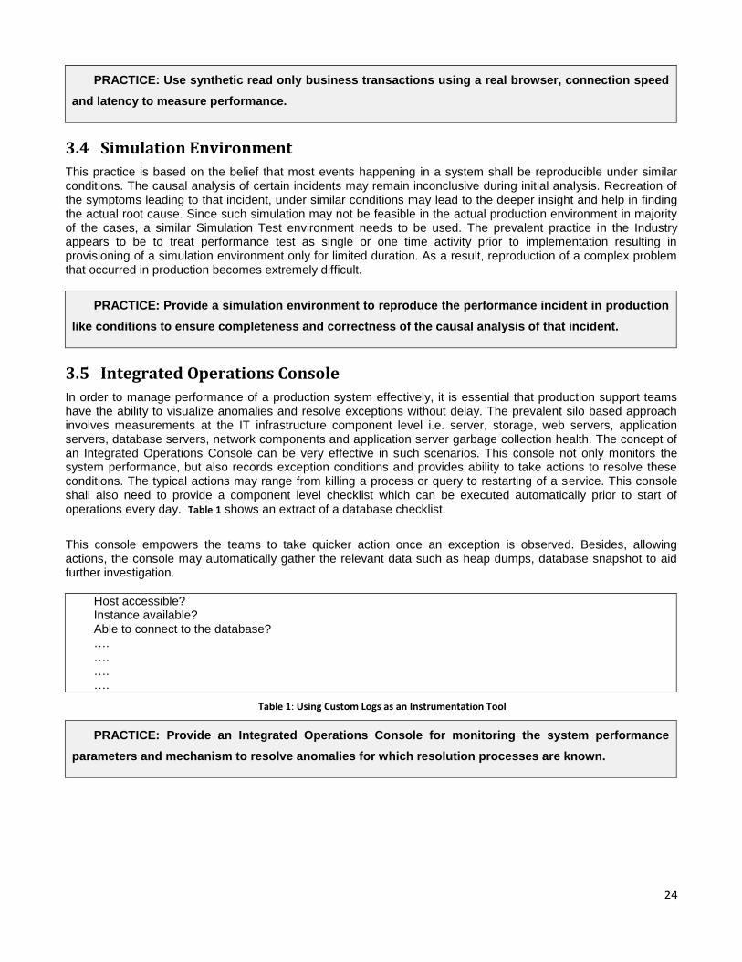
4.1 Implementation 1

The instrumentation was implemented as an integral part of the design and design activity of the e-governance application. Figure 6 shows the instrumentation implemented in that application. The tiers 2, 2A, 3, 5 and 6 implemented instrumentation in the form of web server logs and custom logs. The tiers 2B and 4 implemented instrumentation in the form of database snapshots. The relevant logs from all tiers all collected at a shared location. The information from these logs are processed and used as input to the System Performance Archive and Integration Operations Console.

Figure 6: Instrumentation implemented in web server, application server and database

The first example shows how simple instrumentation helped finding the cause of a performance incident in where end users experienced high response time. Figure 7 and Figure 8 show request and response time graphs of tier 1 and 3 respectively calculated using the web server logs and depicted on the Integrated Operations Console. The request is the count of all the requests serviced in a given time interval and the response time is the mean execution time of all the requests serviced in that time interval. The visual inspection of Figure 7 clearly shows a high mean response time in tier 1. The spike in the mean response time is not visible in tier 3 for the same duration, but there is drop in the number of request serviced by this tier. This helps us to conclude that the origin of the performance incident may be tier 1 or 2A.

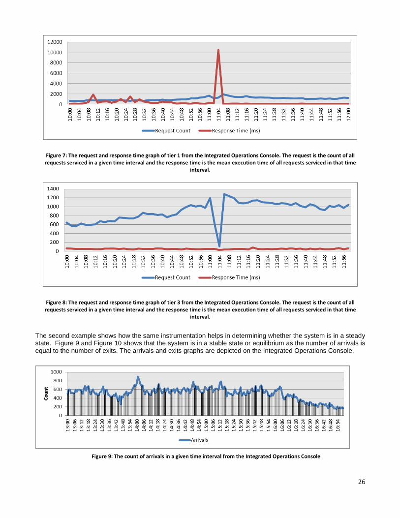
26

Figure 7: The request and response time graph of tier 1 from the Integrated Operations Console. The request is the count of all requests serviced in a given time interval and the response time is the mean execution time of all requests serviced in that time

interval.

Figure 8: The request and response time graph of tier 3 from the Integrated Operations Console. The request is the count of all requests serviced in a given time interval and the response time is the mean execution time of all requests serviced in that time

interval.

The second example shows how the same instrumentation helps in determining whether the system is in a steady state. Figure 9 and Figure 10 shows that the system is in a stable state or equilibrium as the number of arrivals is equal to the number of exits. The arrivals and exits graphs are depicted on the Integrated Operations Console.

Figure 9: The count of arrivals in a given time interval from the Integrated Operations Console

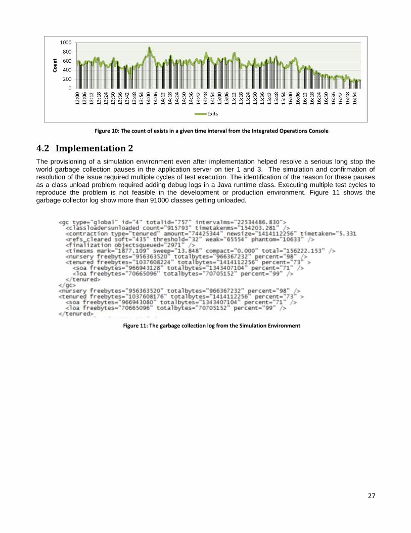
27

Figure 10: The count of exists in a given time interval from the Integrated Operations Console

4.2 Implementation 2

The provisioning of a simulation environment even after implementation helped resolve a serious long stop the world garbage collection pauses in the application server on tier 1 and 3. The simulation and confirmation of resolution of the issue required multiple cycles of test execution. The identification of the reason for these pauses as a class unload problem required adding debug logs in a Java runtime class. Executing multiple test cycles to reproduce the problem is not feasible in the development or production environment. Figure 11 shows the garbage collector log show more than 91000 classes getting unloaded.

Figure 11: The garbage collection log from the Simulation Environment

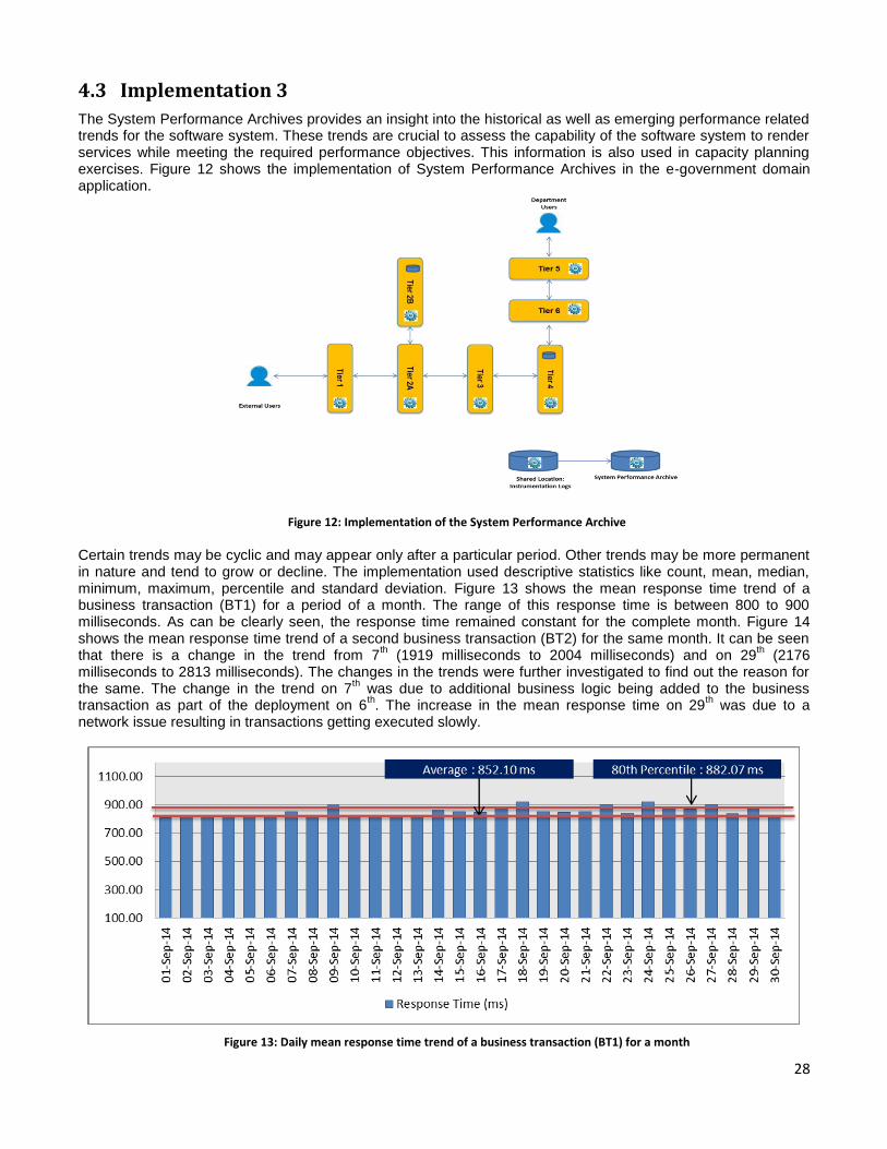
28

4.3 Implementation 3

The System Performance Archives provides an insight into the historical as well as emerging performance related trends for the software system. These trends are crucial to assess the capability of the software system to render services while meeting the required performance objectives. This information is also used in capacity planning exercises. Figure 12 shows the implementation of System Performance Archives in the e-government domain application.

Figure 12: Implementation of the System Performance Archive

Certain trends may be cyclic and may appear only after a particular period. Other trends may be more permanent in nature and tend to grow or decline. The implementation used descriptive statistics like count, mean, median, minimum, maximum, percentile and standard deviation. Figure 13 shows the mean response time trend of a business transaction (BT1) for a period of a month. The range of this response time is between 800 to 900 milliseconds. As can be clearly seen, the response time remained constant for the complete month. Figure 14 shows the mean response time trend of a second business transaction (BT2) for the same month. It can be seen that there is a change in the trend from 7

th (1919 milliseconds to 2004 milliseconds) and on 29

th (2176

milliseconds to 2813 milliseconds). The changes in the trends were further investigated to find out the reason for the same. The change in the trend on 7

th was due to additional business logic being added to the business

transaction as part of the deployment on 6th. The increase in the mean response time on 29

th was due to a

network issue resulting in transactions getting executed slowly.

Figure 13: Daily mean response time trend of a business transaction (BT1) for a month

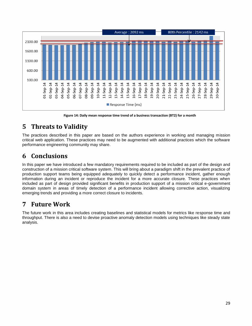
29

Figure 14: Daily mean response time trend of a business transaction (BT2) for a month

5 Threats to Validity The practices described in this paper are based on the authors experience in working and managing mission critical web application. These practices may need to be augmented with additional practices which the software performance engineering community may share.

6 Conclusions In this paper we have introduced a few mandatory requirements required to be included as part of the design and construction of a mission critical software system. This will bring about a paradigm shift in the prevalent practice of production support teams being equipped adequately to quickly detect a performance incident, gather enough information during an incident or reproduce the incident for a more accurate closure. These practices when included as part of design provided significant benefits in production support of a mission critical e-government domain system in areas of timely detection of a performance incident allowing corrective action, visualizing emerging trends and providing a more correct closure to incidents.

7 Future Work The future work in this area includes creating baselines and statistical models for metrics like response time and throughput. There is also a need to devise proactive anomaly detection models using techniques like steady state analysis.

30

References

[YOGE2009] K. K. Aggarwal and Yogesh Singh, “Software Engineering”, New Age International Publishers, p470, 2009.

[SIMI2008] B. Simic, "The Performance of Web Applications: Customers Are Won or Lost in One Second", Technical Report - Aberdeen Group, Accessed on 31 Jan 2014 at http://www.aberdeen.com/aberdeen-library/5136/RA-performance-web-application.aspx

[SATO2010] S. Iwata and K. Kono, Narrowing Down Possible Causes of Performance Anomaly in Web Applications, European Dependable Computing Conference, p185-190, 2010.

[CONN2002] Connie U. Smith, Performance Solutions – A practical guide to creating responsive, scalable software, Addison Wesley, p243, 2002.

[BREW1996] Brewster Kahle, Internet Archives, Accessed on 17 Aug 2014 at http://en.wikipedia.org/wiki/Brewster_Kahle

[HTPA2011] http archive, Accessed on 31 Jan 2014 at http://httparchive.org/

[WPGT] WebPageTest, Accessed on 31 Oct 2014 at https://sites.google.com/a/webpagetest.org/docs/private-instances

The copyright of this paper is owned by the author(s). The author(s) hereby grants Computer Measurement Group Inc a royalty

free right to publish this paper in CMG India Annual Conference Proceedings. 31

Incremental Risk Charge Calculation: A case study of

performance optimization on many/multi core

platforms

Amit Kalele*, Manoj Nambiar# and Mahesh Barve

*#

Center of Excellence for Optimization and Parallelization

Tata Consultancy Services Limited, Pune India

*kalele.amit@tcs.com,

#m.nambiar@tcs.com,

*#mahesh.barve@tcs.com

Incremental Risk Charge calculation is a crucial part of credit risk estimation. This data intensive

calculation requires huge compute resources. A large grid of workstations was deployed at a large

European bank to carry out these computations. In this paper we show that with availability of many

core coprocessors like GPU and MIC and parallel computing paradigms, speed up of order of

magnitude can be achieved for the same workload with just a single server. This proof of concept

demonstrates that with the help of performance analysis and tuning, coprocessors can be made to

deliver high performance with low energy consumption, making them a “must-have” for financial

institutions.

1. Introduction Incremental Risk Charge (IRC) is a regulatory charge for default and migration risk for trading

book position. Inclusion of IRC is made mandatory under the new Basel III reforms in banking

regulations for minimum trading book capital. The calculation of IRC is a compute intensive

task, especially the methods involving Monte-Carlo simulations. A large European bank

approached us to analyze and resolve performance bottlenecks in IRC calculations. The timing

reported on a grid of 50 workstations at their datacenter was approximately 45 min. Risk

estimation and Monte Carlo techniques is well studied topic and details can be found in [1], [2],

[3] and [4]. In this paper we focus on the performance optimization of the IRC calculations on

modern day many/multi core platforms.

The modern day CPUs and GPUs (Graphic Processing Units) are extremely powerful machines.

Equipped with many compute cores, they are capable of performing multiple tasks in parallel.

Exploiting their parallel processing capabilities along with several other optimization techniques,

could result in many fold improvement in performance. In this paper we present our approach for

performance optimization of IRC calculations. We show that multifold gains, in terms of

reduction in compute time, hardware footprint and energy required, can be achieved. We report

that 13.5x and 5.2x speed up is achieved on Nvidia’s K40 GPUs and Intel KNC coprocessor

respectively.

In this paper we present performance optimization of IRC calculations on Nvidia’s K40 [11] and

Intel’s Xeon Phi or KNC coprocessors. We also present benchmarks on Intel’s latest available

platforms namely Sandy Bridge and Ivy Bridge processors. The paper is organized as follows. In

the next section (2), we briefly describe incremental risk charge in relations with credit risk. In

section (3) & (4), we introduce a method for the IRC calculation along with the experimental

setup and procedure. The performance optimization of IRC calculation on Nvidia’s K40 and

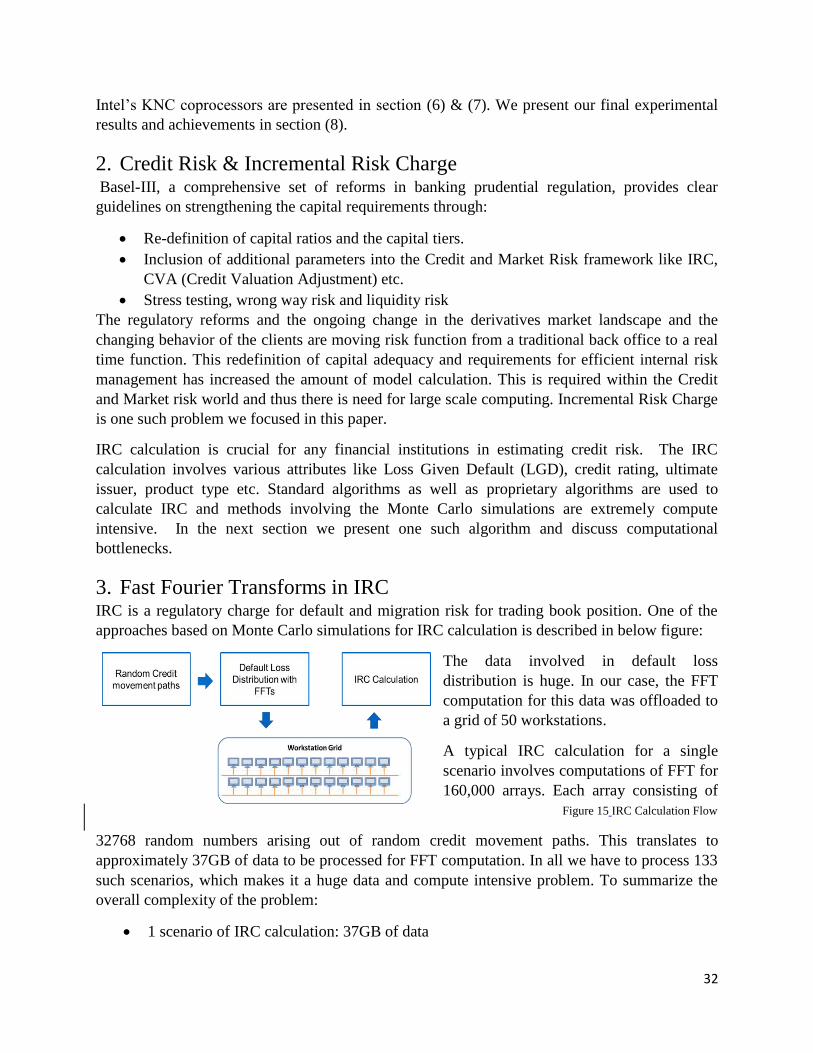
32

Intel’s KNC coprocessors are presented in section (6) & (7). We present our final experimental

results and achievements in section (8).

2. Credit Risk & Incremental Risk Charge Basel-III, a comprehensive set of reforms in banking prudential regulation, provides clear

guidelines on strengthening the capital requirements through:

Re-definition of capital ratios and the capital tiers.

Inclusion of additional parameters into the Credit and Market Risk framework like IRC,

CVA (Credit Valuation Adjustment) etc.

Stress testing, wrong way risk and liquidity risk

The regulatory reforms and the ongoing change in the derivatives market landscape and the

changing behavior of the clients are moving risk function from a traditional back office to a real

time function. This redefinition of capital adequacy and requirements for efficient internal risk

management has increased the amount of model calculation. This is required within the Credit

and Market risk world and thus there is need for large scale computing. Incremental Risk Charge

is one such problem we focused in this paper.

IRC calculation is crucial for any financial institutions in estimating credit risk. The IRC

calculation involves various attributes like Loss Given Default (LGD), credit rating, ultimate

issuer, product type etc. Standard algorithms as well as proprietary algorithms are used to

calculate IRC and methods involving the Monte Carlo simulations are extremely compute

intensive. In the next section we present one such algorithm and discuss computational

bottlenecks.

3. Fast Fourier Transforms in IRC IRC is a regulatory charge for default and migration risk for trading book position. One of the

approaches based on Monte Carlo simulations for IRC calculation is described in below figure:

The data involved in default loss

distribution is huge. In our case, the FFT

computation for this data was offloaded to

a grid of 50 workstations.

A typical IRC calculation for a single

scenario involves computations of FFT for

160,000 arrays. Each array consisting of

32768 random numbers arising out of random credit movement paths. This translates to

approximately 37GB of data to be processed for FFT computation. In all we have to process 133

such scenarios, which makes it a huge data and compute intensive problem. To summarize the

overall complexity of the problem:

1 scenario of IRC calculation: 37GB of data

Figure 15 IRC Calculation Flow

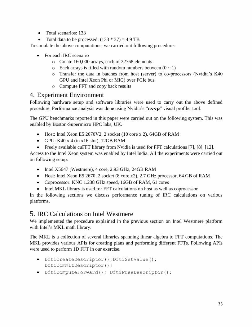
33

Total scenarios: 133

Total data to be processed: (133 * 37) = 4.9 TB

To simulate the above computations, we carried out following procedure:

For each IRC scenario

o Create 160,000 arrays, each of 32768 elements

o Each arrays is filled with random numbers between (0 ~ 1)

o Transfer the data in batches from host (server) to co-processors (Nvidia’s K40

GPU and Intel Xeon Phi or MIC) over PCIe bus

o Compute FFT and copy back results

4. Experiment Environment Following hardware setup and software libraries were used to carry out the above defined

procedure. Performance analysis was done using Nvidia’s “nvvp” visual profiler tool.

The GPU benchmarks reported in this paper were carried out on the following system. This was

enabled by Boston-Supermicro HPC labs, UK.

Host: Intel Xeon E5 2670V2, 2 socket (10 core x 2), 64GB of RAM

GPU: K40 x 4 (in x16 slot), 12GB RAM

Freely available cuFFT library from Nvidia is used for FFT calculations [7], [8], [12].

Access to the Intel Xeon system was enabled by Intel India. All the experiments were carried out

on following setup.

Intel X5647 (Westmere), 4 core, 2.93 GHz, 24GB RAM

Host: Intel Xeon E5 2670, 2 socket (8 core x2), 2.7 GHz processor, 64 GB of RAM

Coprocessor: KNC 1.238 GHz speed, 16GB of RAM, 61 cores

Intel MKL library is used for FFT calculations on host as well as coprocessor

In the following sections we discuss performance tuning of IRC calculations on various

platforms.

5. IRC Calculations on Intel Westmere We implemented the procedure explained in the previous section on Intel Westmere platform

with Intel’s MKL math library.

The MKL is a collection of several libraries spanning linear algebra to FFT computations. The

MKL provides various APIs for creating plans and performing different FFTs. Following APIs

were used to perform 1D FFT in our exercise.

DftiCreateDescriptor();DftiSetValue();

DftiCommitDescriptor();

DftiComputeForward(); DftiFreeDescriptor();

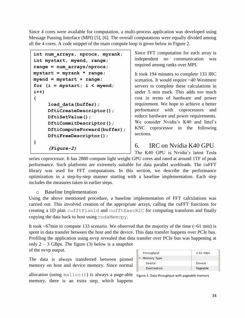
34

Since 4 cores were available for computation, a multi-process application was developed using

Message Passing Interface (MPI) [5], [6]. The overall computations were equally divided among

all the 4 cores. A code snippet of the main compute loop is given below in Figure 2.

Since FFT computation for each array is

independent no communication was

required among ranks over MPI.

It took 194 minutes to complete 133 IRC

scenarios. It would require ~40 Westmere

servers to complete these calculations in

under 5 min mark. This adds too much

cost in terms of hardware and power

requirement. We hope to achieve a better

performance with coprocessors and

reduce hardware and power requirements.

We consider Nvidia’s K40 and Intel’s

KNC coprocessor in the following

sections.

6. IRC on Nvidia K40 GPU The K40 GPU is Nvidia’s latest Tesla

series coprocessor. It has 2880 compute light weight GPU cores and rated at around 1TF of peak

performance. Such platforms are extremely suitable for data parallel workloads. The cuFFT

library was used for FFT computations. In this section, we describe the performance

optimization in a step-by-step manner starting with a baseline implementation. Each step

includes the measures taken in earlier steps.

o Baseline Implementation

Using the above mentioned procedure, a baseline implementation of FFT calculations was

carried out. This involved creation of the appropriate arrays, calling the cuFFT functions for

creating a 1D plan cufftPlan1d and cufftExecR2C for computing transform and finally

copying the data back to host using cudaMemcpy.

It took ~67min to compute 133 scenario. We observed that the majority of the time (~61 min) is

spent in data transfer between the host and the device. This data transfer happens over PCIe bus.

Profiling the application using nvvp revealed that data transfer over PCIe bus was happening at

only 2 – 3 GBps. The figure (3) below is a snapshot

of the nvvp output.

The data is always transferred between pinned

memory on host and device memory. Since normal

allocation (using malloc()) is always a page-able

memory, there is an extra step, which happens

int num_arrays, nprocs, myrank;

int mystart, myend, range;

range = num_arrays/nprocs;

mystart = myrank * range;

myend = mystart + range;

for (i = mystart; i < myend;

i++)

{

load_data(buffer);

DftiCreateDescriptor();

DftiSetValue();

DftiCommitDescriptor();

DftiComputeForward(buffer);

DftiFreeDescriptor();

}

(Figure-2)

Figure 3. Data throughput with pageable memory

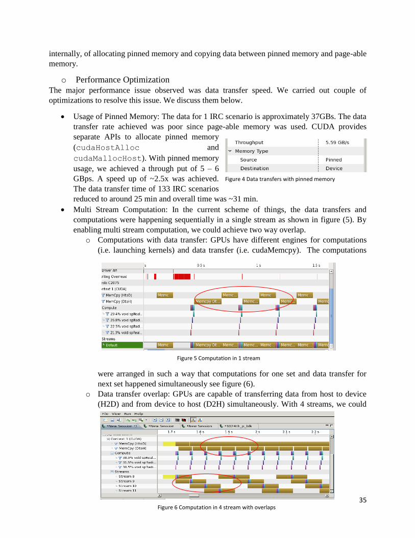
35

internally, of allocating pinned memory and copying data between pinned memory and page-able

memory.

o Performance Optimization

The major performance issue observed was data transfer speed. We carried out couple of

optimizations to resolve this issue. We discuss them below.

Usage of Pinned Memory: The data for 1 IRC scenario is approximately 37GBs. The data

transfer rate achieved was poor since page-able memory was used. CUDA provides

separate APIs to allocate pinned memory

(cudaHostAlloc and

cudaMallocHost). With pinned memory

usage, we achieved a through put of 5 – 6

GBps. A speed up of ~2.5x was achieved.

The data transfer time of 133 IRC scenarios

reduced to around 25 min and overall time was ~31 min.

Multi Stream Computation: In the current scheme of things, the data transfers and

computations were happening sequentially in a single stream as shown in figure (5). By

enabling multi stream computation, we could achieve two way overlap. o Computations with data transfer: GPUs have different engines for computations

(i.e. launching kernels) and data transfer (i.e. cudaMemcpy). The computations

were arranged in such a way that computations for one set and data transfer for

next set happened simultaneously see figure (6). o Data transfer overlap: GPUs are capable of transferring data from host to device

(H2D) and from device to host (D2H) simultaneously. With 4 streams, we could

Figure 4 Data transfers with pinned memory

Figure 5 Computation in 1 stream

Figure 6 Computation in 4 stream with overlaps

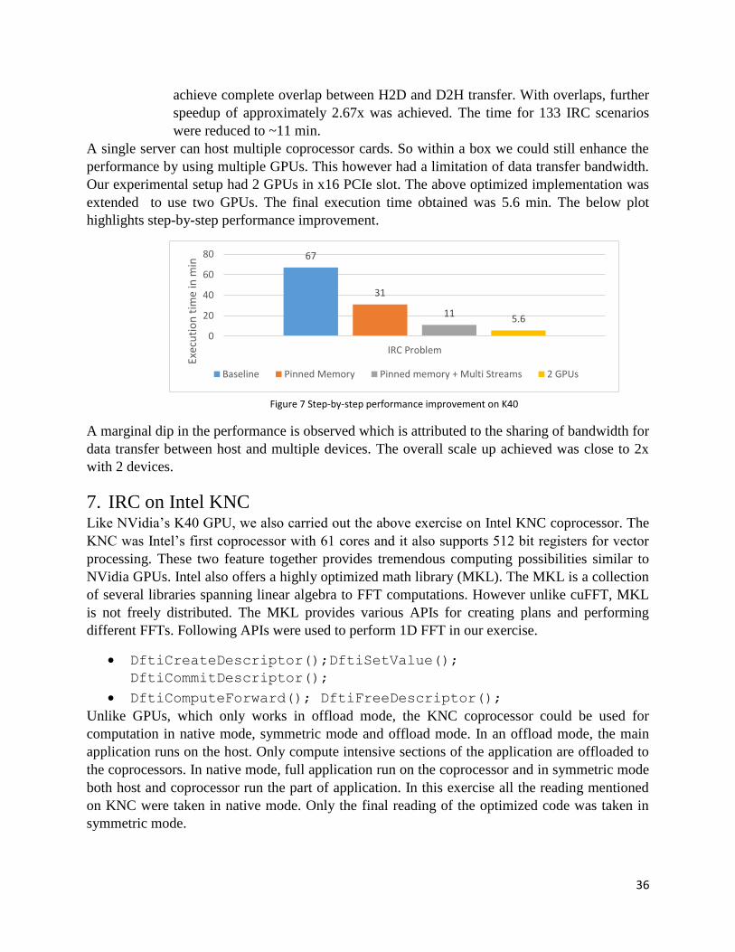
36

achieve complete overlap between H2D and D2H transfer. With overlaps, further

speedup of approximately 2.67x was achieved. The time for 133 IRC scenarios

were reduced to ~11 min. A single server can host multiple coprocessor cards. So within a box we could still enhance the

performance by using multiple GPUs. This however had a limitation of data transfer bandwidth.

Our experimental setup had 2 GPUs in x16 PCIe slot. The above optimized implementation was

extended to use two GPUs. The final execution time obtained was 5.6 min. The below plot

highlights step-by-step performance improvement.

A marginal dip in the performance is observed which is attributed to the sharing of bandwidth for

data transfer between host and multiple devices. The overall scale up achieved was close to 2x

with 2 devices.

7. IRC on Intel KNC Like NVidia’s K40 GPU, we also carried out the above exercise on Intel KNC coprocessor. The

KNC was Intel’s first coprocessor with 61 cores and it also supports 512 bit registers for vector

processing. These two feature together provides tremendous computing possibilities similar to

NVidia GPUs. Intel also offers a highly optimized math library (MKL). The MKL is a collection

of several libraries spanning linear algebra to FFT computations. However unlike cuFFT, MKL

is not freely distributed. The MKL provides various APIs for creating plans and performing

different FFTs. Following APIs were used to perform 1D FFT in our exercise.

DftiCreateDescriptor();DftiSetValue();

DftiCommitDescriptor();

DftiComputeForward(); DftiFreeDescriptor();

Unlike GPUs, which only works in offload mode, the KNC coprocessor could be used for

computation in native mode, symmetric mode and offload mode. In an offload mode, the main

application runs on the host. Only compute intensive sections of the application are offloaded to

the coprocessors. In native mode, full application run on the coprocessor and in symmetric mode

both host and coprocessor run the part of application. In this exercise all the reading mentioned

on KNC were taken in native mode. Only the final reading of the optimized code was taken in

symmetric mode.

67

31

11 5.6

0

20

40

60

80

IRC Problem

Exec

uti

on

tim

e in

min

Baseline Pinned Memory Pinned memory + Multi Streams 2 GPUs

Figure 7 Step-by-step performance improvement on K40

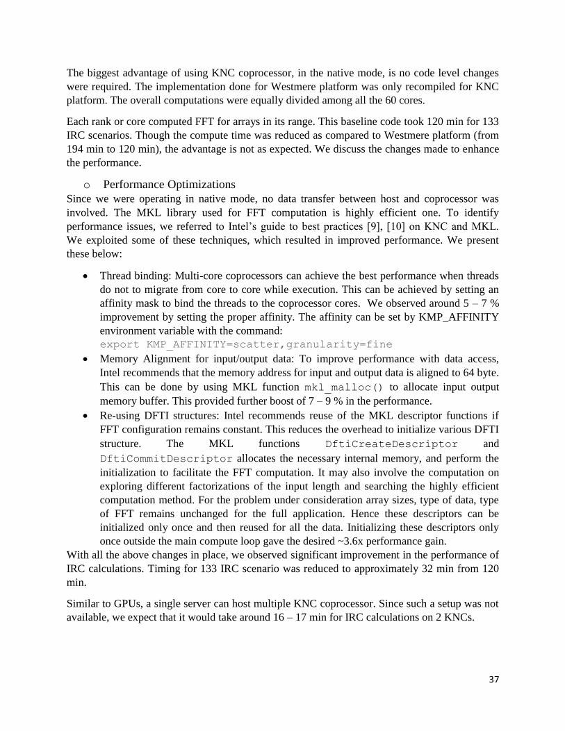
37

The biggest advantage of using KNC coprocessor, in the native mode, is no code level changes

were required. The implementation done for Westmere platform was only recompiled for KNC

platform. The overall computations were equally divided among all the 60 cores.

Each rank or core computed FFT for arrays in its range. This baseline code took 120 min for 133

IRC scenarios. Though the compute time was reduced as compared to Westmere platform (from

194 min to 120 min), the advantage is not as expected. We discuss the changes made to enhance

the performance.

o Performance Optimizations

Since we were operating in native mode, no data transfer between host and coprocessor was

involved. The MKL library used for FFT computation is highly efficient one. To identify

performance issues, we referred to Intel’s guide to best practices [9], [10] on KNC and MKL.

We exploited some of these techniques, which resulted in improved performance. We present

these below:

Thread binding: Multi-core coprocessors can achieve the best performance when threads

do not to migrate from core to core while execution. This can be achieved by setting an

affinity mask to bind the threads to the coprocessor cores. We observed around 5 – 7 %

improvement by setting the proper affinity. The affinity can be set by KMP_AFFINITY

environment variable with the command:

export KMP_AFFINITY=scatter,granularity=fine

Memory Alignment for input/output data: To improve performance with data access,

Intel recommends that the memory address for input and output data is aligned to 64 byte.

This can be done by using MKL function mkl_malloc() to allocate input output

memory buffer. This provided further boost of 7 – 9 % in the performance.

Re-using DFTI structures: Intel recommends reuse of the MKL descriptor functions if

FFT configuration remains constant. This reduces the overhead to initialize various DFTI

structure. The MKL functions DftiCreateDescriptor and

DftiCommitDescriptor allocates the necessary internal memory, and perform the

initialization to facilitate the FFT computation. It may also involve the computation on

exploring different factorizations of the input length and searching the highly efficient

computation method. For the problem under consideration array sizes, type of data, type

of FFT remains unchanged for the full application. Hence these descriptors can be

initialized only once and then reused for all the data. Initializing these descriptors only

once outside the main compute loop gave the desired ~3.6x performance gain.

With all the above changes in place, we observed significant improvement in the performance of

IRC calculations. Timing for 133 IRC scenario was reduced to approximately 32 min from 120

min.

Similar to GPUs, a single server can host multiple KNC coprocessor. Since such a setup was not

available, we expect that it would take around 16 – 17 min for IRC calculations on 2 KNCs.

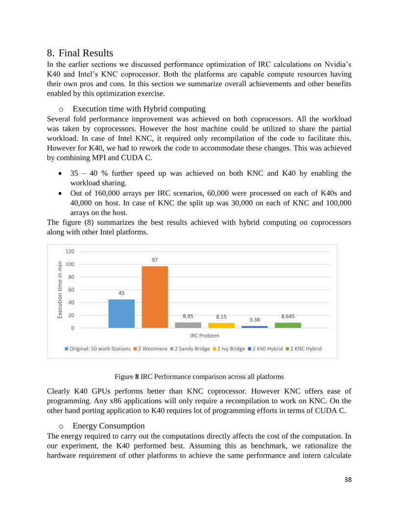
38

8. Final Results In the earlier sections we discussed performance optimization of IRC calculations on Nvidia’s

K40 and Intel’s KNC coprocessor. Both the platforms are capable compute resources having

their own pros and cons. In this section we summarize overall achievements and other benefits

enabled by this optimization exercise.

o Execution time with Hybrid computing

Several fold performance improvement was achieved on both coprocessors. All the workload

was taken by coprocessors. However the host machine could be utilized to share the partial

workload. In case of Intel KNC, it required only recompilation of the code to facilitate this.

However for K40, we had to rework the code to accommodate these changes. This was achieved

by combining MPI and CUDA C.

35 – 40 % further speed up was achieved on both KNC and K40 by enabling the

workload sharing.

Out of 160,000 arrays per IRC scenarios, 60,000 were processed on each of K40s and

40,000 on host. In case of KNC the split up was 30,000 on each of KNC and 100,000

arrays on the host.

The figure (8) summarizes the best results achieved with hybrid computing on coprocessors

along with other Intel platforms.

Figure 8 IRC Performance comparison across all platforms

Clearly K40 GPUs performs better than KNC coprocessor. However KNC offers ease of

programming. Any x86 applications will only require a recompilation to work on KNC. On the

other hand porting application to K40 requires lot of programming efforts in terms of CUDA C.

o Energy Consumption

The energy required to carry out the computations directly affects the cost of the computation. In

our experiment, the K40 performed best. Assuming this as benchmark, we rationalize the

hardware requirement of other platforms to achieve the same performance and intern calculate

45

97

8.95 8.15 3.38

8.645

0

20

40

60

80

100

120

IRC Problem

Exec

uti

on

tim

e in

min

Original: 50 work Stations 2 Westmere 2 Sandy Bridge 2 Ivy Bridge 2 K40 Hybrid 2 KNC Hybrid

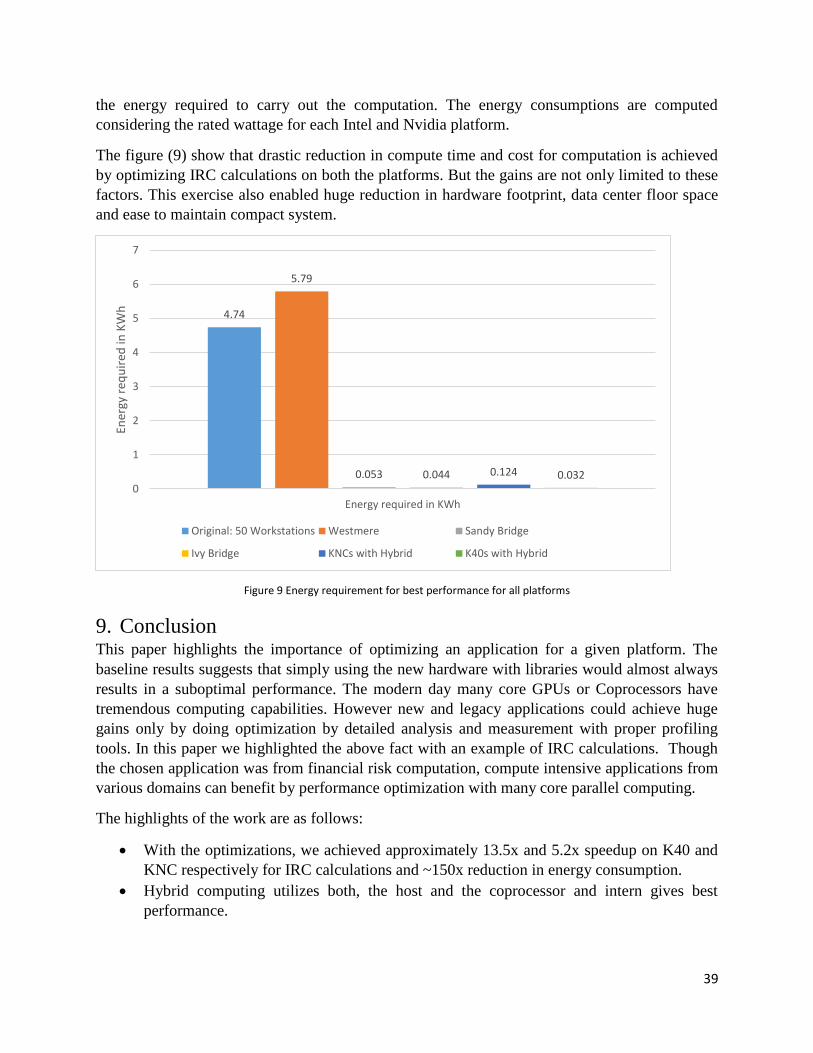
39

the energy required to carry out the computation. The energy consumptions are computed

considering the rated wattage for each Intel and Nvidia platform.

The figure (9) show that drastic reduction in compute time and cost for computation is achieved

by optimizing IRC calculations on both the platforms. But the gains are not only limited to these

factors. This exercise also enabled huge reduction in hardware footprint, data center floor space

and ease to maintain compact system.

Figure 9 Energy requirement for best performance for all platforms

9. Conclusion This paper highlights the importance of optimizing an application for a given platform. The

baseline results suggests that simply using the new hardware with libraries would almost always

results in a suboptimal performance. The modern day many core GPUs or Coprocessors have

tremendous computing capabilities. However new and legacy applications could achieve huge

gains only by doing optimization by detailed analysis and measurement with proper profiling

tools. In this paper we highlighted the above fact with an example of IRC calculations. Though

the chosen application was from financial risk computation, compute intensive applications from

various domains can benefit by performance optimization with many core parallel computing.

The highlights of the work are as follows:

With the optimizations, we achieved approximately 13.5x and 5.2x speedup on K40 and

KNC respectively for IRC calculations and ~150x reduction in energy consumption.

Hybrid computing utilizes both, the host and the coprocessor and intern gives best

performance.

4.74

5.79

0.053 0.044 0.124 0.032 0

1

2

3

4

5

6

7

Energy required in KWh

Ener

gy r

equ

ired

in K

Wh

Original: 50 Workstations Westmere Sandy Bridge

Ivy Bridge KNCs with Hybrid K40s with Hybrid

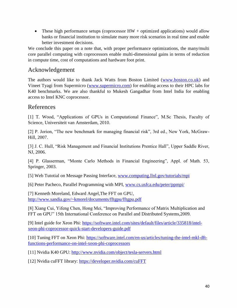
40

These high performance setups (coprocessor HW + optimized applications) would allow

banks or financial institution to simulate many more risk scenarios in real time and enable

better investment decisions.

We conclude this paper on a note that, with proper performance optimizations, the many/multi

core parallel computing with coprocessors enable multi-dimensional gains in terms of reduction

in compute time, cost of computations and hardware foot print.

Acknowledgement

The authors would like to thank Jack Watts from Boston Limited (www.boston.co.uk) and

Vineet Tyagi from Supermicro (www.supermicro.com) for enabling access to their HPC labs for

K40 benchmarks. We are also thankful to Mukesh Gangadhar from Intel India for enabling

access to Intel KNC coprocessor.

References

[1] T. Wood, “Applications of GPUs in Computational Finance”, M.Sc Thesis, Faculty of

Science, Universiteit van Amsterdam, 2010.

[2] P. Jorion, “The new benchmark for managing financial risk”, 3rd ed., New York, McGraw-

Hill, 2007.

[3] J. C. Hull, “Risk Management and Financial Institutions Prentice Hall”, Upper Saddle River,

NJ, 2006.

[4] P. Glasserman, “Monte Carlo Methods in Financial Engineering”, Appl. of Math. 53,

Springer, 2003.

[5] Web Tutotial on Message Passing Interface, www.computing.llnl.gov/tutorials/mpi

[6] Peter Pacheco, Parallel Programming with MPI, www.cs.usfca.edu/peter/ppmpi/

[7] Kenneth Moreland, Edward Angel,The FFT on GPU,

http://www.sandia.gov/~kmorel/documents/fftgpu/fftgpu.pdf

[8] Xiang Cui, Yifeng Chen, Hong Mei, “Improving Performance of Matrix Multiplication and

FFT on GPU” 15th International Conference on Parallel and Distributed Systems,2009.

[9] Intel guide for Xeon Phi: https://software.intel.com/sites/default/files/article/335818/intel-

xeon-phi-coprocessor-quick-start-developers-guide.pdf

[10] Tuning FFT on Xeon Phi: https://software.intel.com/en-us/articles/tuning-the-intel-mkl-dft-

functions-performance-on-intel-xeon-phi-coprocessors

[11] Nvidia K40 GPU: http://www.nvidia.com/object/tesla-servers.html

[12] Nvidia cuFFT library: https://developer.nvidia.com/cuFFT

The copyright of this paper is owned by the author(s). The author(s) hereby grants Computer Measurement Group Inc a royalty free right to publish this paper in CMG India Annual Conference Proceedings.

41

Performance Benchmarking for Open Source Message Productions

Yogesh Bhate Abhay Pendse Deepti Nagarkar Performance Engg. Group Performance Engg. Group Performance Engg. Group

Persistent Systems Persistent Systems Persistent Systems yogesh_bhate@persistent.co.in abhay_pendse@persistent.co.in deepti_nagarkar@persistent.co.in

Abstract- This paper shares the experiences and findings that were collected during a 6-month

performance benchmarking activity carried out on multiple open source messaging products. The primary

aim of the activity was to identify the best performant messaging product from around 5 shortlisted

messaging products available in the open source community. There were specific requirements provided

against which the benchmarking activity was carried out. This paper covers the objective, the plan and

the execution methodology followed for this. The paper also shares the detailed numbers that were

captured during the tests.

1. Introduction

A large scale telescope system is being built by a consortium of 4-5 countries. The telescope system

consists of the actual manufacturing, installation and the operation of a 30 Meter telescope and its related

software sub systems. All software subsystems that control the telescope or use the output provided by

the telescope need to communicate with each other through a backbone set of services providing multiple

common functionalities like logging, security, monitoring and messaging. Messaging or Event Service as

it is called is one the primary service which is part of the backbone infrastructure in the telescope software

system. Each software subcomponent talks to one another use a set of events and those events need to

be propogated to the correct target in real-time.

The event service backbone had stringent performance requirements which are listed in subsequent

sections. The event service was planned to be a thin API layer over a well-known open source messaging

product. This allowed the software planners to keep an option open of changing the middleware in the

lifecycle of the event service. It was required that the software lifecycle would be a minimum of 30 years

from the date of commissioning of the telescope systems. Benchmarking open source messaging

platforms for use in the Event Service development was the primary goal of this project

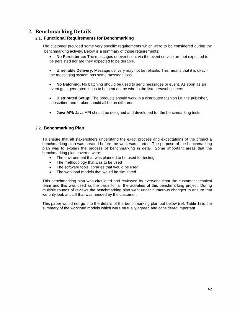
42

2. Benchmarking Details 2.1. Functional Requirements for Benchmarking

The customer provided some very specific requirements which were to be considered during the

benchmarking activity. Below is a summary of those requirements:

No Persistence: The messages or event sent via the event service are not expected to be persisted nor are they expected to be durable.

Unreliable Delivery: Message delivery may not be reliable. This means that it is okay if the messaging system has some message loss.

No Batching: No batching should be used to send messages or event. As soon as an event gets generated it has to be sent on the wire to the listeners/subscribers.

Distributed Setup: The products should work in a distributed fashion i.e. the publisher, subscriber, and broker should all be on different.

Java API: Java API should be designed and developed for the benchmarking tests.

2.2. Benchmarking Plan

To ensure that all stakeholders understand the exact process and expectations of the project a benchmarking plan was created before the work was started. The purpose of the benchmarking plan was to explain the process of benchmarking in detail. Some important areas that the benchmarking plan covered were:

The environment that was planned to be used for testing

The methodology that was to be used

The software tools, libraries that would be used.

The workload models that would be simulated This benchmarking plan was circulated and reviewed by everyone from the customer technical team and this was used as the basis for all the activities of this benchmarking project. During multiple rounds of reviews the benchmarking plan went under numerous changes to ensure that we only look at stuff that was needed by the customer. This paper would not go into the details of the benchmarking plan but below (ref. Table 1) is the summary of the workload models which were mutually agreed and considered important

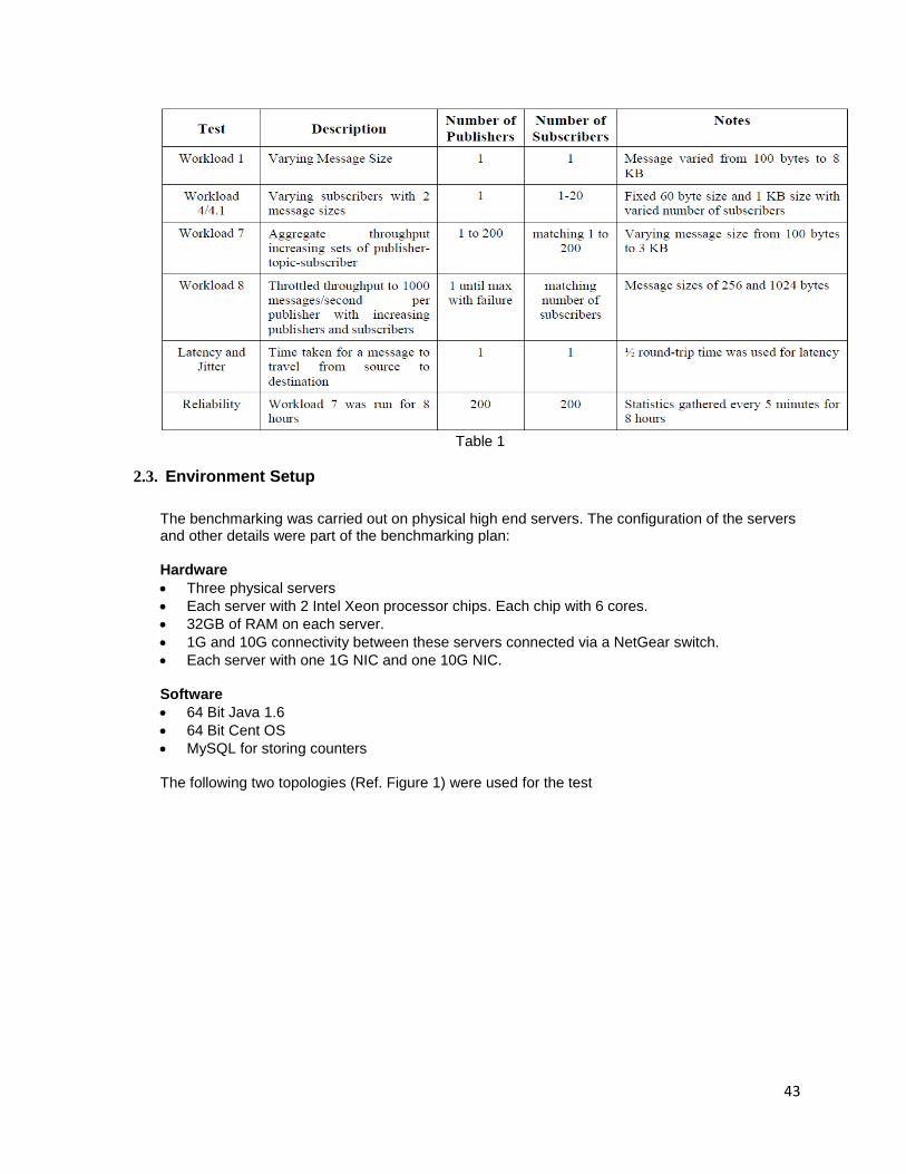
43

Table 1

2.3. Environment Setup

The benchmarking was carried out on physical high end servers. The configuration of the servers and other details were part of the benchmarking plan:

Hardware

Three physical servers

Each server with 2 Intel Xeon processor chips. Each chip with 6 cores.

32GB of RAM on each server.

1G and 10G connectivity between these servers connected via a NetGear switch.

Each server with one 1G NIC and one 10G NIC.

Software

64 Bit Java 1.6

64 Bit Cent OS

MySQL for storing counters The following two topologies (Ref. Figure 1) were used for the test

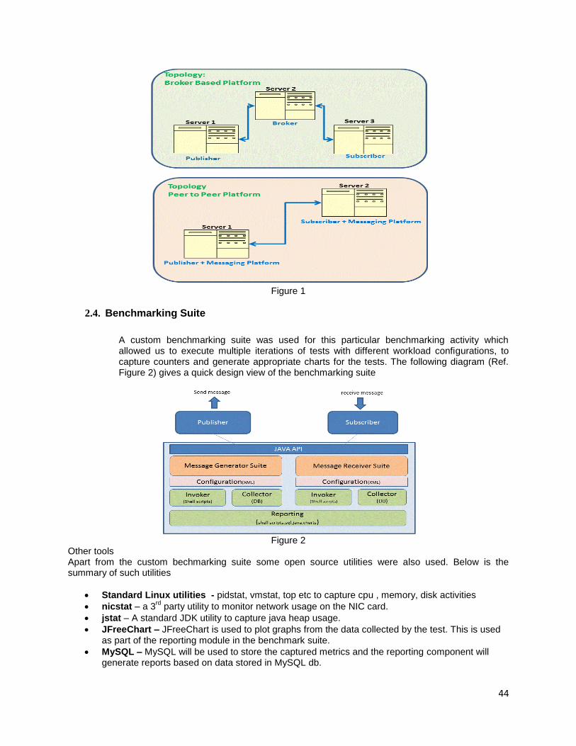
44

Figure 1

2.4. Benchmarking Suite

A custom benchmarking suite was used for this particular benchmarking activity which allowed us to execute multiple iterations of tests with different workload configurations, to capture counters and generate appropriate charts for the tests. The following diagram (Ref. Figure 2) gives a quick design view of the benchmarking suite

Figure 2

Other tools Apart from the custom bechmarking suite some open source utilities were also used. Below is the summary of such utilities

Standard Linux utilities - pidstat, vmstat, top etc to capture cpu , memory, disk activities

nicstat – a 3rd

party utility to monitor network usage on the NIC card.

jstat – A standard JDK utility to capture java heap usage.

JFreeChart – JFreeChart is used to plot graphs from the data collected by the test. This is used as part of the reporting module in the benchmark suite.

MySQL – MySQL will be used to store the captured metrics and the reporting component will generate reports based on data stored in MySQL db.

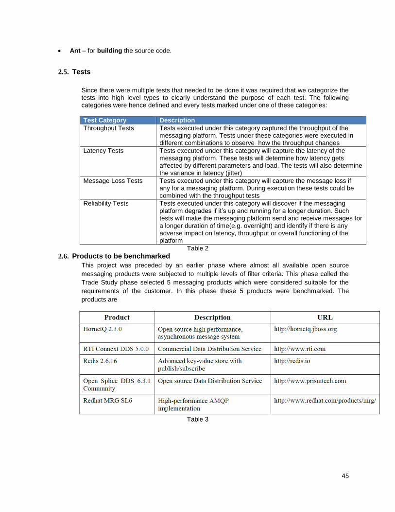
45

Ant – for building the source code.

2.5. Tests

Since there were multiple tests that needed to be done it was required that we categorize the tests into high level types to clearly understand the purpose of each test. The following categories were hence defined and every tests marked under one of these categories:

Test Category Description

Throughput Tests Tests executed under this category captured the throughput of the messaging platform. Tests under these categories were executed in different combinations to observe how the throughput changes

Latency Tests Tests executed under this category will capture the latency of the messaging platform. These tests will determine how latency gets affected by different parameters and load. The tests will also determine the variance in latency (jitter)

Message Loss Tests Tests executed under this category will capture the message loss if any for a messaging platform. During execution these tests could be combined with the throughput tests

Reliability Tests Tests executed under this category will discover if the messaging platform degrades if it’s up and running for a longer duration. Such tests will make the messaging platform send and receive messages for a longer duration of time(e.g. overnight) and identify if there is any adverse impact on latency, throughput or overall functioning of the platform

Table 2

2.6. Products to be benchmarked

This project was preceded by an earlier phase where almost all available open source

messaging products were subjected to multiple levels of filter criteria. This phase called the

Trade Study phase selected 5 messaging products which were considered suitable for the

requirements of the customer. In this phase these 5 products were benchmarked. The

products are

Table 3

46

2.7. Reporting

It was decided that the following important quantitative parameters would be reported after

the benchmarking tests. For all 5 products each of these parameters would be compared and

the product which has the best values for the majority of the parameters would be chosen.

Publisher Throughput – Max Number of messages sent per second

Subscriber Throughput – Max Number of messages received per second

Latency – The time taken for the message from point A to point B.

Jitter – Variation in Latency

Message Loss – Loss of messages

Important Note: All the tests were to be done on 1G and 10G network. It was decided that for

comparison purposes the numbers observed for a 10G network would be used since the

production network bandwidth was planned to be 10G.

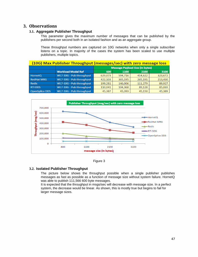
47

3. Observations 3.1. Aggregate Publisher Throughput

This parameter gives the maximum number of messages that can be published by the publishers per second both in an isolated fashion and as an aggregate group. These throughput numbers are captured on 10G networks when only a single subscriber listens on a topic. In majority of the cases the system has been scaled to use multiple publishers, multiple topics.

Figure 3

3.2. Isolated Publisher Throughput

The picture below shows the throughput possible when a single publisher publishes messages as fast as possible as a function of message size without system failure. HornetQ was able to publish 111,566 600 byte messages. It is expected that the throughput in msgs/sec will decrease with message size. In a perfect system, the decrease would be linear. As shown, this is mostly true but begins to fail for larger message sizes.

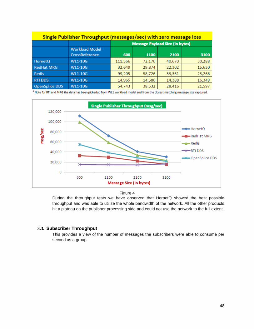
48

Figure 4

During the throughput tests we have observed that HornetQ showed the best possible

throughput and was able to utilize the whole bandwidth of the network. All the other products

hit a plateau on the publisher processing side and could not use the network to the full extent.

3.3. Subscriber Throughput

This provides a view of the number of messages the subscribers were able to consume per

second as a group.

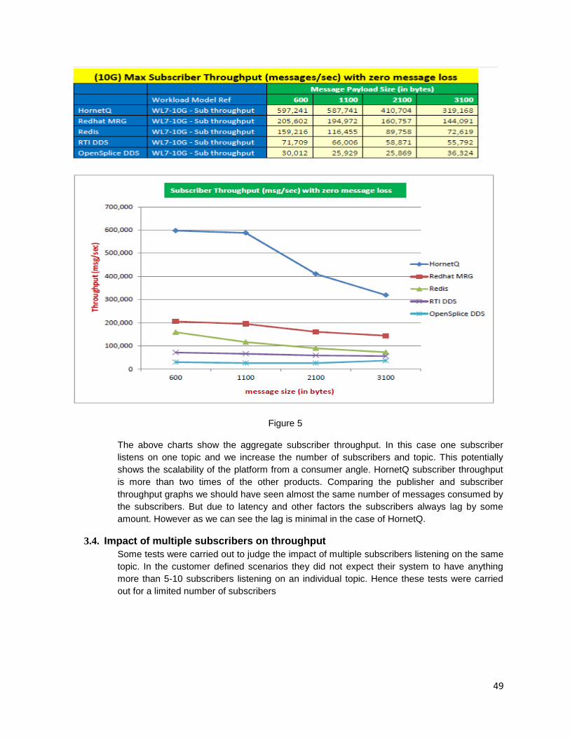
49

Figure 5

The above charts show the aggregate subscriber throughput. In this case one subscriber

listens on one topic and we increase the number of subscribers and topic. This potentially

shows the scalability of the platform from a consumer angle. HornetQ subscriber throughput

is more than two times of the other products. Comparing the publisher and subscriber

throughput graphs we should have seen almost the same number of messages consumed by

the subscribers. But due to latency and other factors the subscribers always lag by some

amount. However as we can see the lag is minimal in the case of HornetQ.

3.4. Impact of multiple subscribers on throughput

Some tests were carried out to judge the impact of multiple subscribers listening on the same

topic. In the customer defined scenarios they did not expect their system to have anything

more than 5-10 subscribers listening on an individual topic. Hence these tests were carried

out for a limited number of subscribers

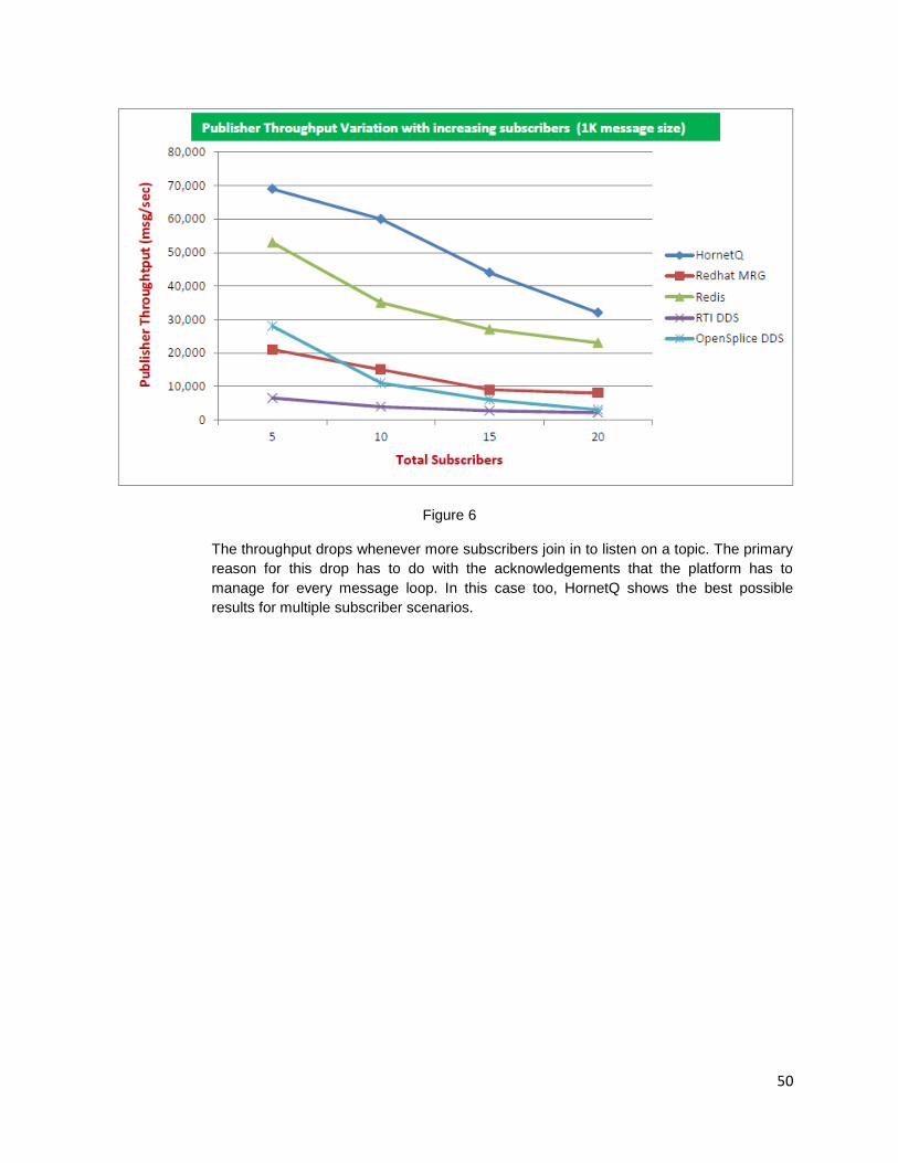
50

Figure 6

The throughput drops whenever more subscribers join in to listen on a topic. The primary

reason for this drop has to do with the acknowledgements that the platform has to

manage for every message loop. In this case too, HornetQ shows the best possible

results for multiple subscriber scenarios.

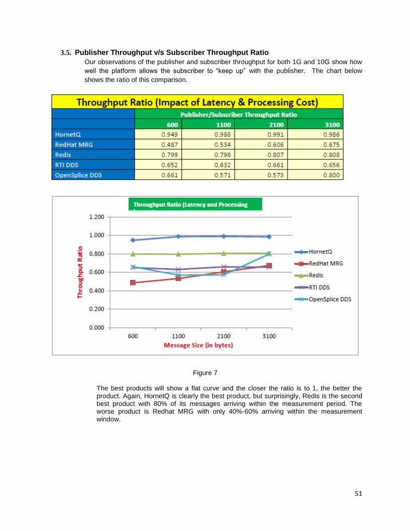
51

3.5. Publisher Throughput v/s Subscriber Throughput Ratio

Our observations of the publisher and subscriber throughput for both 1G and 10G show how

well the platform allows the subscriber to “keep up” with the publisher. The chart below

shows the ratio of this comparison.

Figure 7

The best products will show a flat curve and the closer the ratio is to 1, the better the product. Again, HornetQ is clearly the best product, but surprisingly, Redis is the second best product with 80% of its messages arriving within the measurement period. The worse product is Redhat MRG with only 40%-60% arriving within the measurement window.

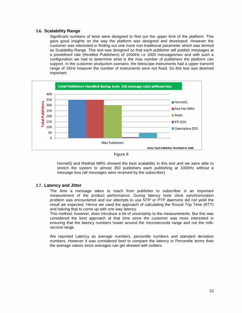
52

3.6. Scalability Range

Significant numbers of tests were designed to find out the upper limit of the platform. This gave good insights on the way the platform was designed and developed. However the customer was interested in finding out one more non-traditional parameter which was termed as Scalability Range. This test was designed so that each publisher will publish messages at a predefined rate (throttled Publishers) of 1000Hz i.e 1000 messages/sec and with such a configuration we had to determine what is the max number of publishers the platform can support. In the customer production scenario, the telescope instruments had a upper transmit range of 1KHz however the number of instruments were not fixed. So this test was deemed important.

Figure 8

HornetQ and RedHat MRG showed the best scalability in this test and we were able to stretch the system to almost 350 publishers each publishing at 1000Hz without a message loss (all messages were received by the subscriber)

3.7. Latency and Jitter

The time a message takes to reach from publisher to subscriber is an important measurement of the product performance. During latency tests clock synchronization problem was encountered and our attempts to use NTP or PTP daemons did not yeild the result we expected. Hence we used the approach of calculating the Round Trip Time (RTT) and halving that to come up with one way latency. This method, however, does introduce a bit of uncertainty to the measurements. But this was considered the best approach at that time since the customer was more interested in ensuring that the latency numbers hower around the microseconds range and not the milli-second range. We reported Latency as average numbers, percentile numbers and standard deviation numbers. However it was considered best to compare the latency in Percentile terms than the average values since averages can get skewed with outliers.

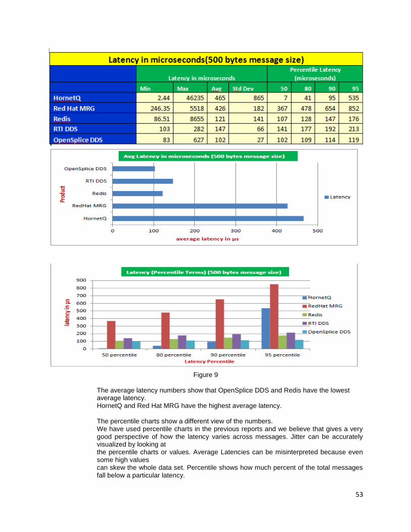
53

Figure 9

The average latency numbers show that OpenSplice DDS and Redis have the lowest average latency. HornetQ and Red Hat MRG have the highest average latency. The percentile charts show a different view of the numbers. We have used percentile charts in the previous reports and we believe that gives a very good perspective of how the latency varies across messages. Jitter can be accurately visualized by looking at the percentile charts or values. Average Latencies can be misinterpreted because even some high values can skew the whole data set. Percentile shows how much percent of the total messages fall below a particular latency.

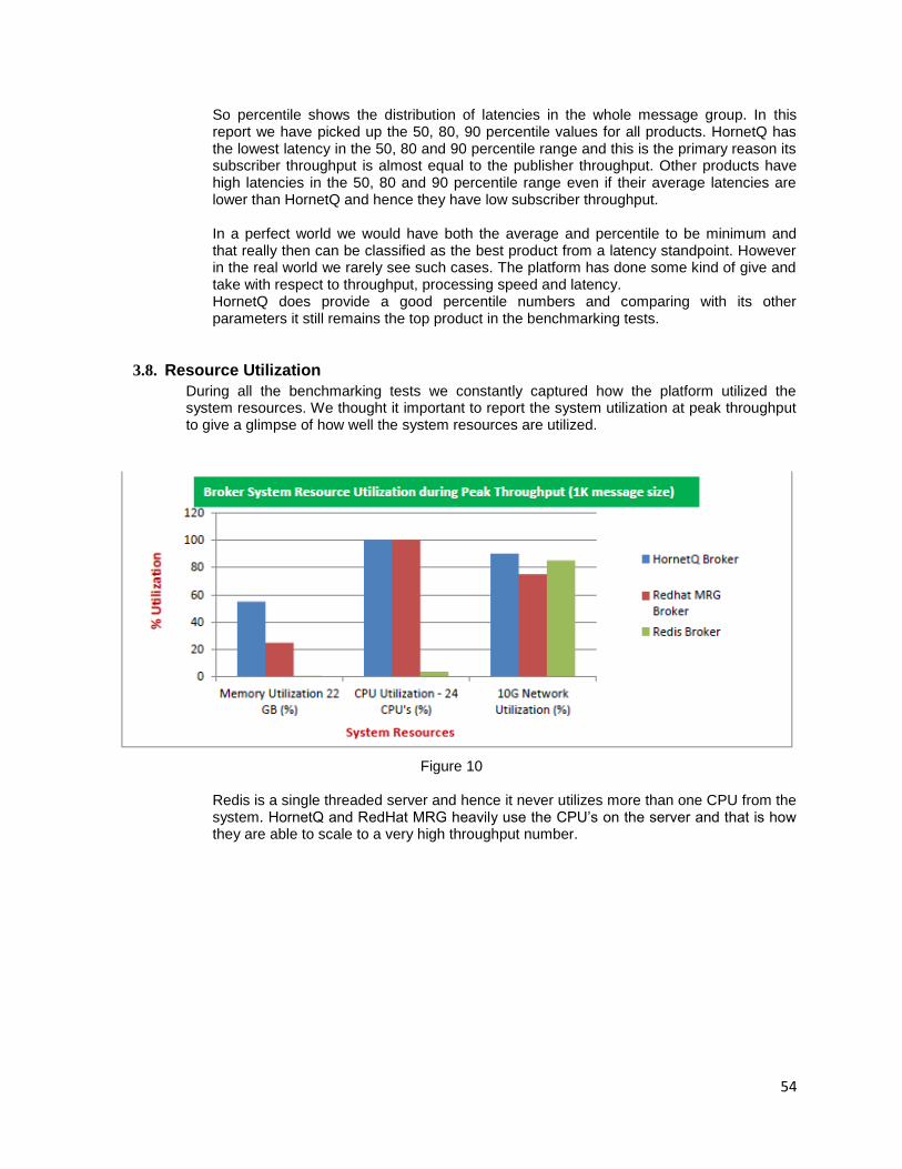
54

So percentile shows the distribution of latencies in the whole message group. In this report we have picked up the 50, 80, 90 percentile values for all products. HornetQ has the lowest latency in the 50, 80 and 90 percentile range and this is the primary reason its subscriber throughput is almost equal to the publisher throughput. Other products have high latencies in the 50, 80 and 90 percentile range even if their average latencies are lower than HornetQ and hence they have low subscriber throughput.

In a perfect world we would have both the average and percentile to be minimum and that really then can be classified as the best product from a latency standpoint. However in the real world we rarely see such cases. The platform has done some kind of give and take with respect to throughput, processing speed and latency. HornetQ does provide a good percentile numbers and comparing with its other parameters it still remains the top product in the benchmarking tests.

3.8. Resource Utilization

During all the benchmarking tests we constantly captured how the platform utilized the system resources. We thought it important to report the system utilization at peak throughput to give a glimpse of how well the system resources are utilized.

Figure 10

Redis is a single threaded server and hence it never utilizes more than one CPU from the system. HornetQ and RedHat MRG heavily use the CPU’s on the server and that is how they are able to scale to a very high throughput number.

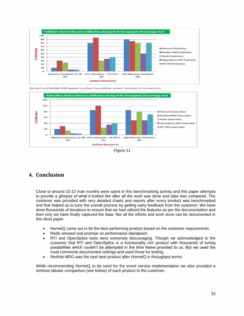
55

Figure 11

4. Conclusion

Close to around 10-12 man months were spent in this benchmarking activity and this paper attempts to provide a glimpse of what it looked like after all the work was done and data was compared. The customer was provided with very detailed charts and reports after every product was benchmarked and that helped us to tune the overall process by getting early feedback from the customer. We have done thousands of iterations to ensure that we had utilized the features as per the documentation and then only we have finally captured the data. Not all the efforts and work done can be documented in this short paper.

HornetQ came out to be the best performing product based on the customer requirements.

Redis showed real promise on performance standpoint.

RTI and OpenSplice tests were extremely discouraging. Though we acknowledged to the customer that RTI and OpenSplice is a functionality rich product with thousands of tuning possibilities which couldn’t be attempted in the time frame provided to us. But we used the most commonly documented settings and used those for testing.

RedHat MRG was the next best product after HornetQ in throughput terms.

While recommending HornetQ to be used for the event service implementation we also provided a verbose tabular comparison (see below) of each product to the customer.

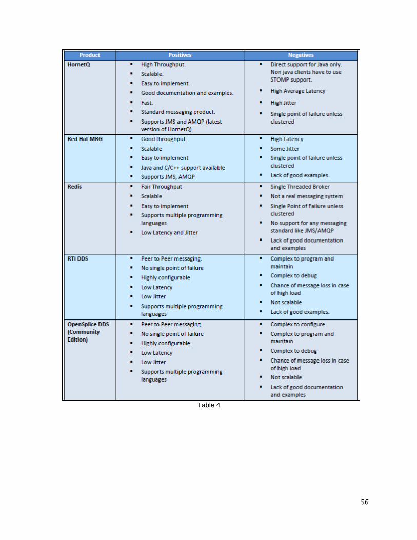
56

Table 4

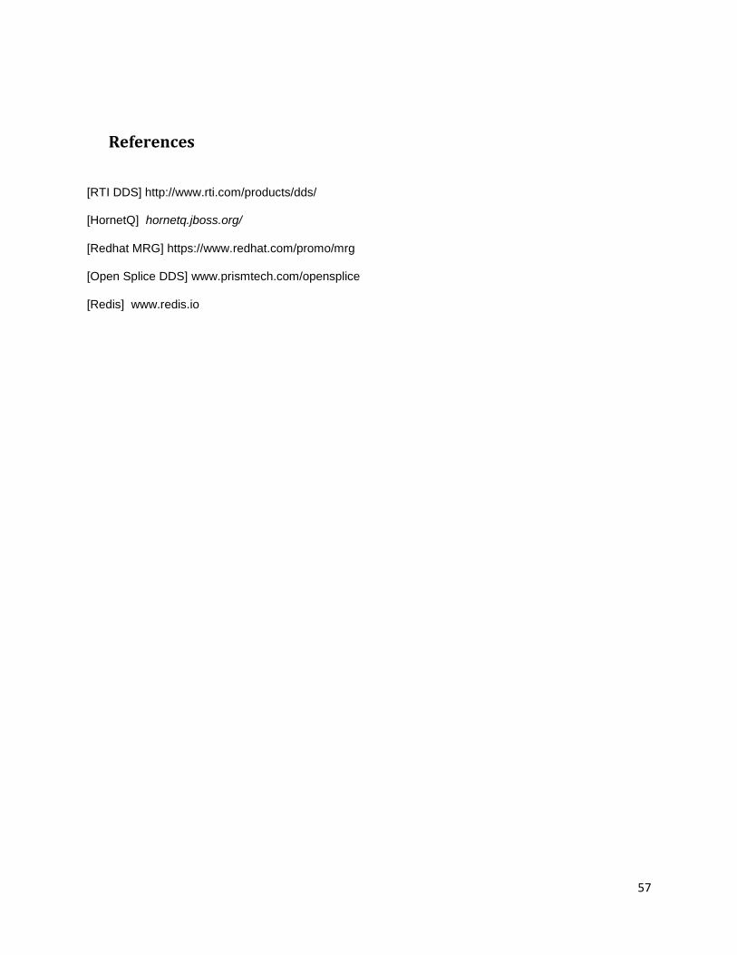
57

References

[RTI DDS] http://www.rti.com/products/dds/

[HornetQ] hornetq.jboss.org/

[Redhat MRG] https://www.redhat.com/promo/mrg

[Open Splice DDS] www.prismtech.com/opensplice

[Redis] www.redis.io

The copyright of this paper is owned by the author(s). The author(s) hereby grants Computer Measurement Group Inc a royalty free right to publish this paper in CMG India Annual Conference Proceedings

AUTOMATICALLY DETERMINING LOAD TEST DURATION USING CONFIDENCE INTERVALS

Rajesh Mansharamani Subhasri Duttagupta Anuja Nehete Freelance Consultant Innovation Labs Perf. Engg. Performance Engg. Group

Tata Consultancy Services Persistent Systems rajesh.mansharamani@gmail.com subhasri.duttagupta@tcs.com anuja_nehete@persistent.co.in

Load testing has become the de facto standard to evaluate performance of applications in the IT industry, thanks to the growing popularity of automated load testing tools. These tools report performance metrics such as average response time and throughput, which are sensitive to the test duration specified by the tester. Too short a duration can lead to inaccurate estimates of performance and too long a duration leads to reduced number of cycles of load testing. Currently, no scientific methodology is followed by load testers to specify run duration. In this paper, we present a simple methodology, using confidence intervals, such that a load test can automatically determine when to converge. We demonstrate the methodology using five lab applications and three real world applications.

1. Introduction

Performance testing (PT) has grown in popularity in the IT industry thanks to a number of commercial and free load testing tools available in the market. These tools let the load tester script application transactions to create virtual users, which mimic the behaviour of real users. At load test execution time, the tester can specify the number of virtual users, the think time (time spent at terminal), and the test duration.

Test duration is specified in these tools either as an absolute time interval or in terms of number of user iterations that need to be tested. In the absence of statistical knowledge, the common practice in the IT industry is to specify an ad hoc duration which may range from a few seconds to a few hours. The ad hoc duration is usually arrived at in consultation with one's test manager or blindly adopted from 'best practices' followed by the PT team.

Regardless of the duration specified, at the end of the load test the tester gets numeric estimates of performance metrics such as average response time and throughput. The numeric value is accepted as true because it has come from a well-known tool. Unfortunately, the sensitivity of test duration on test output is not considered in a regular load test. By regular load test we mean a test that is used to determine the application response time under a given load, and not the stability of the application under load for a long duration (such as to test for memory leaks).

If the test duration is too small the estimate of performance may be erroneous. If the test duration is too long it will lead to fewer cycles for load testing. This paper proposes a simple methodology based on confidence intervals for automatically determining load test duration while a load test is in progress.

Confidence intervals are widely used to determine convergence of discrete event simulations [PAWL1990] [ROBI2007] [EICK2007]. Using confidence intervals one can specify with what probability (say 99%) the estimate of average response time lies in an interval around the true average. The wider the interval less is the confidence in the estimate. As the run duration increases one expects the interval to become tighter and converge to a specified limit (for example, 10% of the true mean). We have not come across any study that

58

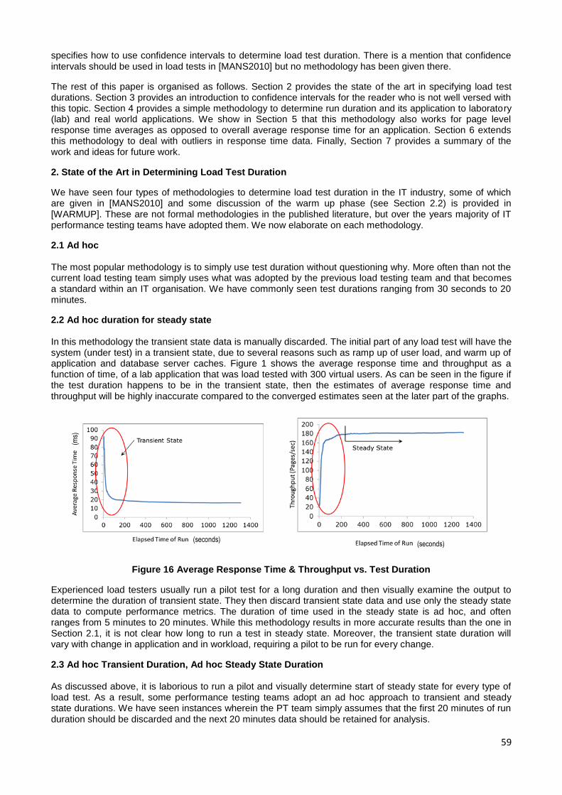
59

specifies how to use confidence intervals to determine load test duration. There is a mention that confidence intervals should be used in load tests in [MANS2010] but no methodology has been given there.

The rest of this paper is organised as follows. Section 2 provides the state of the art in specifying load test durations. Section 3 provides an introduction to confidence intervals for the reader who is not well versed with this topic. Section 4 provides a simple methodology to determine run duration and its application to laboratory (lab) and real world applications. We show in Section 5 that this methodology also works for page level response time averages as opposed to overall average response time for an application. Section 6 extends this methodology to deal with outliers in response time data. Finally, Section 7 provides a summary of the work and ideas for future work.

2. State of the Art in Determining Load Test Duration

We have seen four types of methodologies to determine load test duration in the IT industry, some of which are given in [MANS2010] and some discussion of the warm up phase (see Section 2.2) is provided in [WARMUP]. These are not formal methodologies in the published literature, but over the years majority of IT performance testing teams have adopted them. We now elaborate on each methodology.

2.1 Ad hoc The most popular methodology is to simply use test duration without questioning why. More often than not the current load testing team simply uses what was adopted by the previous load testing team and that becomes a standard within an IT organisation. We have commonly seen test durations ranging from 30 seconds to 20 minutes.

2.2 Ad hoc duration for steady state In this methodology the transient state data is manually discarded. The initial part of any load test will have the system (under test) in a transient state, due to several reasons such as ramp up of user load, and warm up of application and database server caches. Figure 1 shows the average response time and throughput as a function of time, of a lab application that was load tested with 300 virtual users. As can be seen in the figure if the test duration happens to be in the transient state, then the estimates of average response time and throughput will be highly inaccurate compared to the converged estimates seen at the later part of the graphs.

Figure 16 Average Response Time & Throughput vs. Test Duration

Experienced load testers usually run a pilot test for a long duration and then visually examine the output to determine the duration of transient state. They then discard transient state data and use only the steady state data to compute performance metrics. The duration of time used in the steady state is ad hoc, and often ranges from 5 minutes to 20 minutes. While this methodology results in more accurate results than the one in Section 2.1, it is not clear how long to run a test in steady state. Moreover, the transient state duration will vary with change in application and in workload, requiring a pilot to be run for every change.

2.3 Ad hoc Transient Duration, Ad hoc Steady State Duration

As discussed above, it is laborious to run a pilot and visually determine start of steady state for every type of load test. As a result, some performance testing teams adopt an ad hoc approach to transient and steady state durations. We have seen instances wherein the PT team simply assumes that the first 20 minutes of run duration should be discarded and the next 20 minutes data should be retained for analysis.

(ms)

(seconds) (seconds)

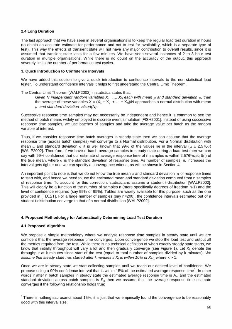
60

2.4 Long Duration The last approach that we have seen in several organisations is to keep the regular load test duration in hours (to obtain an accurate estimate for performance and not to test for availability, which is a separate type of test). This way the effects of transient state will not have any major contribution to overall results, since it is assumed that transient state lasts for a few minutes. We have seen several instances of 2 to 3 hour test duration in multiple organisations. While there is no doubt on the accuracy of the output, this approach severely limits the number of performance test cycles.

3. Quick Introduction to Confidence Intervals

We have added this section to give a quick introduction to confidence intervals to the non-statistical load tester. To understand confidence intervals it helps to first understand the Central Limit Theorem.

The Central Limit Theorem [WALP2002] in statistics states that:

Given N independent random variables X1, …, XN each with mean and standard deviation , then the average of these variables X = (X1 + X2 + … + XN)/N approaches a normal distribution with mean

and standard deviation /sqrt(N).

Successive response time samples may not necessarily be independent and hence it is common to see the method of batch means widely employed in discrete event simulation [FISH2001]. Instead of using successive response time samples, we use batches of samples and take the average value per batch as the random variable of interest.

Thus, if we consider response time batch averages in steady state then we can assume that the average response time (across batch samples) will converge to a Normal distribution. For a Normal distribution with

mean and standard deviation it is well known that 99% of the values lie in the interval ( 2.576) [WALP2002]. Therefore, if we have n batch average samples in steady state during a load test then we can

say with 99% confidence that our estimate of average response time of n samples is within 2.576*/sqrt(n) of

the true mean, where is the standard deviation of response time. As number of samples, n, increases the interval gets tighter and we can specify a convergence criteria, as will be shown in Section 4.

An important point to note is that we do not know the true mean and standard deviation of response times to start with, and hence we need to use the estimated mean and standard deviation computed from n samples of response time. To account for this correction, statisticians assume a student t-distribution [WALP2002]. This will clearly be a function of the number of samples n (more specifically degrees of freedom n-1) and the level of confidence required (say 99% or 95%). Tables are widely available for this purpose, such as the one

provided in [TDIST]. For a large number of samples (say n=200), the confidence intervals estimated out of a student t-distribution converge to that of a normal distribution [WALP2002].

4. Proposed Methodology for Automatically Determining Load Test Duration

4.1 Proposed Algorithm We propose a simple methodology where we analyse response time samples in steady state until we are confident that the average response time converges. Upon convergence we stop the load test and output all the metrics required from the test. While there is no technical definition of when exactly steady state starts, we know that initially throughput will vary a lot and then gradually converge (see Figure 1). Let Xk denote the throughput at k minutes since start of the test (equal to total number of samples divided by k minutes). We

assume that steady state has started after k minutes if Xk is within 10% of Xk-1, where k > 1.

Once we are in steady state we start collecting samples until we reach our desired level of confidence. We

propose using a 99% confidence interval that is within 15% of the estimated average response time1. In other

words if after n batch samples in steady state the estimated average response time is An, and the estimated standard deviation across batch samples is Sn then we assume that the average response time estimate converges if the following relationship holds true:

1 There is nothing sacrosanct about 15%; it is just that we empirically found the convergence to be reasonably

good with this interval size.

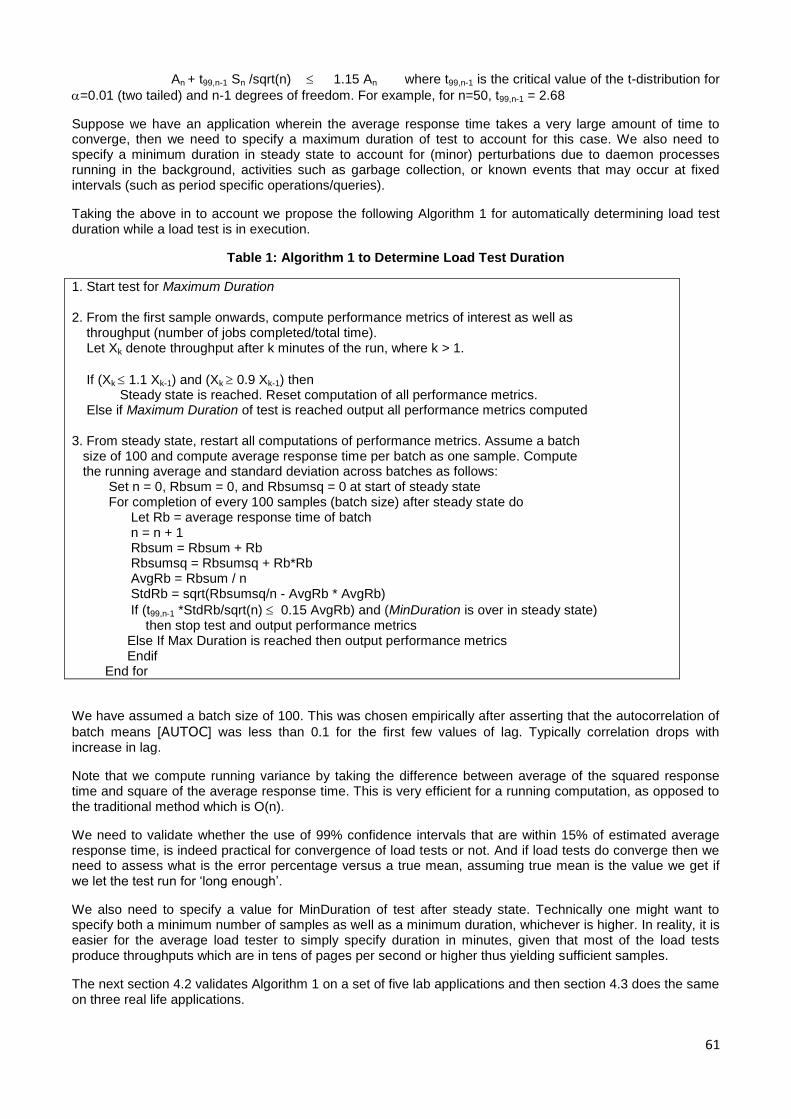
61

An + t99,n-1 Sn /sqrt(n) 1.15 An where t99,n-1 is the critical value of the t-distribution for

=0.01 (two tailed) and n-1 degrees of freedom. For example, for n=50, t99,n-1 = 2.68

Suppose we have an application wherein the average response time takes a very large amount of time to converge, then we need to specify a maximum duration of test to account for this case. We also need to specify a minimum duration in steady state to account for (minor) perturbations due to daemon processes running in the background, activities such as garbage collection, or known events that may occur at fixed intervals (such as period specific operations/queries).

Taking the above in to account we propose the following Algorithm 1 for automatically determining load test duration while a load test is in execution.

Table 1: Algorithm 1 to Determine Load Test Duration

1. Start test for Maximum Duration 2. From the first sample onwards, compute performance metrics of interest as well as throughput (number of jobs completed/total time). Let Xk denote throughput after k minutes of the run, where k > 1.

If (Xk 1.1 Xk-1) and (Xk 0.9 Xk-1) then Steady state is reached. Reset computation of all performance metrics. Else if Maximum Duration of test is reached output all performance metrics computed 3. From steady state, restart all computations of performance metrics. Assume a batch size of 100 and compute average response time per batch as one sample. Compute the running average and standard deviation across batches as follows: Set n = 0, Rbsum = 0, and Rbsumsq = 0 at start of steady state For completion of every 100 samples (batch size) after steady state do Let Rb = average response time of batch n = n + 1 Rbsum = Rbsum + Rb Rbsumsq = Rbsumsq + Rb*Rb AvgRb = Rbsum / n StdRb = sqrt(Rbsumsq/n - AvgRb * AvgRb)

If (t99,n-1 *StdRb/sqrt(n) 0.15 AvgRb) and (MinDuration is over in steady state) then stop test and output performance metrics Else If Max Duration is reached then output performance metrics Endif End for

We have assumed a batch size of 100. This was chosen empirically after asserting that the autocorrelation of

batch means [AUTOC] was less than 0.1 for the first few values of lag. Typically correlation drops with increase in lag.

Note that we compute running variance by taking the difference between average of the squared response time and square of the average response time. This is very efficient for a running computation, as opposed to the traditional method which is O(n).

We need to validate whether the use of 99% confidence intervals that are within 15% of estimated average response time, is indeed practical for convergence of load tests or not. And if load tests do converge then we need to assess what is the error percentage versus a true mean, assuming true mean is the value we get if we let the test run for ‘long enough’.

We also need to specify a value for MinDuration of test after steady state. Technically one might want to specify both a minimum number of samples as well as a minimum duration, whichever is higher. In reality, it is easier for the average load tester to simply specify duration in minutes, given that most of the load tests produce throughputs which are in tens of pages per second or higher thus yielding sufficient samples.

The next section 4.2 validates Algorithm 1 on a set of five lab applications and then section 4.3 does the same on three real life applications.

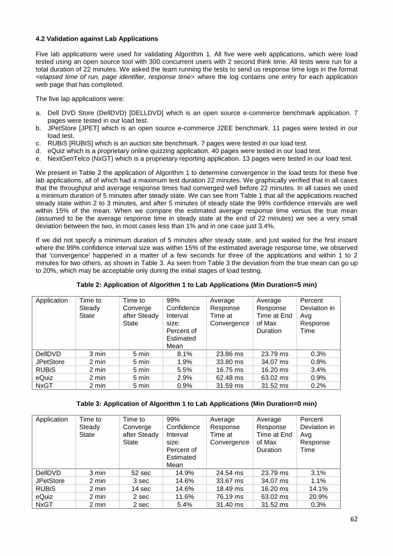
62

4.2 Validation against Lab Applications

Five lab applications were used for validating Algorithm 1. All five were web applications, which were load tested using an open source tool with 300 concurrent users with 2 second think time. All tests were run for a total duration of 22 minutes. We asked the team running the tests to send us response time logs in the format <elapsed time of run, page identifier, response time> where the log contains one entry for each application

web page that has completed.

The five lap applications were:

a. Dell DVD Store (DellDVD) [DELLDVD] which is an open source e-commerce benchmark application. 7 pages were tested in our load test.

b. JPetStore [JPET] which is an open source e-commerce J2EE benchmark. 11 pages were tested in our load test.

c. RUBiS [RUBIS] which is an auction site benchmark. 7 pages were tested in our load test. d. eQuiz which is a proprietary online quizzing application. 40 pages were tested in our load test. e. NextGenTelco (NxGT) which is a proprietary reporting application. 13 pages were tested in our load test.

We present in Table 2 the application of Algorithm 1 to determine convergence in the load tests for these five lab applications, all of which had a maximum test duration 22 minutes. We graphically verified that in all cases that the throughput and average response times had converged well before 22 minutes. In all cases we used a minimum duration of 5 minutes after steady state. We can see from Table 1 that all the applications reached steady state within 2 to 3 minutes, and after 5 minutes of steady state the 99% confidence intervals are well within 15% of the mean. When we compare the estimated average response time versus the true mean (assumed to be the average response time in steady state at the end of 22 minutes) we see a very small deviation between the two, in most cases less than 1% and in one case just 3.4%.

If we did not specify a minimum duration of 5 minutes after steady state, and just waited for the first instant where the 99% confidence interval size was within 15% of the estimated average response time, we observed that 'convergence' happened in a matter of a few seconds for three of the applications and within 1 to 2 minutes for two others, as shown in Table 3. As seen from Table 3 the deviation from the true mean can go up to 20%, which may be acceptable only during the initial stages of load testing.

Table 2: Application of Algorithm 1 to Lab Applications (Min Duration=5 min)

Application Time to Steady State

Time to Converge after Steady State

99% Confidence Interval size: Percent of Estimated Mean

Average Response Time at Convergence

Average Response Time at End of Max Duration

Percent Deviation in Avg Response Time

DellDVD 3 min 5 min 8.1% 23.86 ms 23.79 ms 0.3%

JPetStore 2 min 5 min 1.9% 33.80 ms 34.07 ms 0.8%

RUBiS 2 min 5 min 5.5% 16.75 ms 16.20 ms 3.4%

eQuiz 2 min 5 min 2.9% 62.48 ms 63.02 ms 0.9%

NxGT 2 min 5 min 0.9% 31.59 ms 31.52 ms 0.2%

Table 3: Application of Algorithm 1 to Lab Applications (Min Duration=0 min)

Application Time to Steady State

Time to Converge after Steady State

99% Confidence Interval size: Percent of Estimated Mean

Average Response Time at Convergence

Average Response Time at End of Max Duration

Percent Deviation in Avg Response Time

DellDVD 3 min 52 sec 14.9% 24.54 ms 23.79 ms 3.1%

JPetStore 2 min 3 sec 14.6% 33.67 ms 34.07 ms 1.1%

RUBiS 2 min 14 sec 14.6% 18.49 ms 16.20 ms 14.1%

eQuiz 2 min 2 sec 11.6% 76.19 ms 63.02 ms 20.9%

NxGT 2 min 2 sec 5.4% 31.40 ms 31.52 ms 0.3%

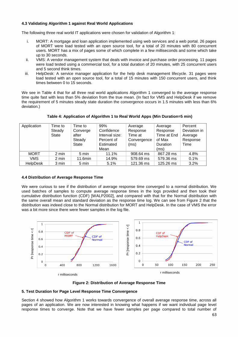
63

4.3 Validating Algorithm 1 against Real World Applications

The following three real world IT applications were chosen for validation of Algorithm 1:

i. MORT: A mortgage and loan application implemented using web services and a web portal. 26 pages of MORT were load tested with an open source tool, for a total of 20 minutes with 80 concurrent users. MORT has a mix of pages some of which complete in a few milliseconds and some which take up to 30 seconds.

ii. VMS: A vendor management system that deals with invoice and purchase order processing. 11 pages were load tested using a commercial tool, for a total duration of 20 minutes, with 25 concurrent users and 5 second think times.

iii. HelpDesk: A service manager application for the help desk management lifecycle. 31 pages were load tested with an open source tool, for a total of 15 minutes with 150 concurrent users, and think times between 0 to 15 seconds.

We see in Table 4 that for all three real world applications Algorithm 1 converged to the average response time quite fast with less than 5% deviation from the true mean. (In fact for VMS and HelpDesk if we remove the requirement of 5 minutes steady state duration the convergence occurs in 1.5 minutes with less than 6% deviation.)

Table 4: Application of Algorithm 1 to Real World Apps (Min Duration=5 min)

Application Time to Steady State

Time to Converge after Steady State

99% Confidence Interval size: Percent of Estimated Mean

Average Response Time at Convergence (ms)

Average Response Time at End of Max Duration (ms)

Percent Deviation in Average Response Time

MORT 2 min 5 min 11.1% 908.64 ms 867.28 ms 4.8%

VMS 2 min 11.6min 14.9% 579.69 ms 579.36 ms 0.1%

HelpDesk 3 min 5 min 5.1% 121.36 ms 125.26 ms 3.2%

4.4 Distribution of Average Response Time We were curious to see if the distribution of average response time converged to a normal distribution. We used batches of samples to compute average response times in the logs provided and then took their cumulative distribution function (CDF) [WALP2002], and compared with that for the Normal distribution with the same overall mean and standard deviation as the response time log. We can see from Figure 2 that the distribution was indeed close to the Normal distribution for MORT and HelpDesk. In the case of VMS the error was a bit more since there were fewer samples in the log file.

Figure 2: Distribution of Average Response Time

5. Test Duration for Page Level Response Time Convergence

Section 4 showed how Algorithm 1 works towards convergence of overall average response time, across all pages of an application. We are now interested in knowing what happens if we want individual page level response times to converge. Note that we have fewer samples per page compared to total number of

Pr

[response tim

e <

r]

r milliseconds r milliseconds

Pr

[response tim

e <

r]

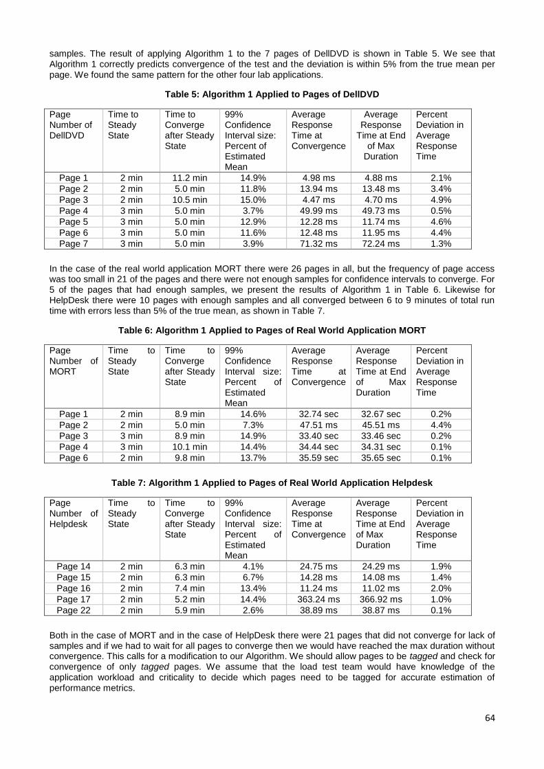
64

samples. The result of applying Algorithm 1 to the 7 pages of DellDVD is shown in Table 5. We see that Algorithm 1 correctly predicts convergence of the test and the deviation is within 5% from the true mean per page. We found the same pattern for the other four lab applications.

Table 5: Algorithm 1 Applied to Pages of DellDVD

Page Number of DellDVD

Time to Steady State

Time to Converge after Steady State

99% Confidence Interval size: Percent of Estimated Mean

Average Response Time at Convergence

Average Response

Time at End of Max

Duration

Percent Deviation in Average Response Time

Page 1 2 min 11.2 min 14.9% 4.98 ms 4.88 ms 2.1%

Page 2 2 min 5.0 min 11.8% 13.94 ms 13.48 ms 3.4%

Page 3 2 min 10.5 min 15.0% 4.47 ms 4.70 ms 4.9%

Page 4 3 min 5.0 min 3.7% 49.99 ms 49.73 ms 0.5%

Page 5 3 min 5.0 min 12.9% 12.28 ms 11.74 ms 4.6%

Page 6 3 min 5.0 min 11.6% 12.48 ms 11.95 ms 4.4%

Page 7 3 min 5.0 min 3.9% 71.32 ms 72.24 ms 1.3%

In the case of the real world application MORT there were 26 pages in all, but the frequency of page access was too small in 21 of the pages and there were not enough samples for confidence intervals to converge. For 5 of the pages that had enough samples, we present the results of Algorithm 1 in Table 6. Likewise for HelpDesk there were 10 pages with enough samples and all converged between 6 to 9 minutes of total run time with errors less than 5% of the true mean, as shown in Table 7.

Table 6: Algorithm 1 Applied to Pages of Real World Application MORT

Page Number of MORT

Time to Steady State

Time to Converge after Steady State

99% Confidence Interval size: Percent of Estimated Mean

Average Response Time at Convergence

Average Response Time at End of Max Duration

Percent Deviation in Average Response Time

Page 1 2 min 8.9 min 14.6% 32.74 sec 32.67 sec 0.2%

Page 2 2 min 5.0 min 7.3% 47.51 ms 45.51 ms 4.4%

Page 3 3 min 8.9 min 14.9% 33.40 sec 33.46 sec 0.2%

Page 4 3 min 10.1 min 14.4% 34.44 sec 34.31 sec 0.1%

Page 6 2 min 9.8 min 13.7% 35.59 sec 35.65 sec 0.1%

Table 7: Algorithm 1 Applied to Pages of Real World Application Helpdesk

Page Number of Helpdesk

Time to Steady State

Time to Converge after Steady State

99% Confidence Interval size: Percent of Estimated Mean

Average Response Time at Convergence

Average Response Time at End of Max Duration

Percent Deviation in Average Response Time

Page 14 2 min 6.3 min 4.1% 24.75 ms 24.29 ms 1.9%

Page 15 2 min 6.3 min 6.7% 14.28 ms 14.08 ms 1.4%

Page 16 2 min 7.4 min 13.4% 11.24 ms 11.02 ms 2.0%

Page 17 2 min 5.2 min 14.4% 363.24 ms 366.92 ms 1.0%

Page 22 2 min 5.9 min 2.6% 38.89 ms 38.87 ms 0.1%

Both in the case of MORT and in the case of HelpDesk there were 21 pages that did not converge for lack of samples and if we had to wait for all pages to converge then we would have reached the max duration without convergence. This calls for a modification to our Algorithm. We should allow pages to be tagged and check for convergence of only tagged pages. We assume that the load test team would have knowledge of the application workload and criticality to decide which pages need to be tagged for accurate estimation of performance metrics.

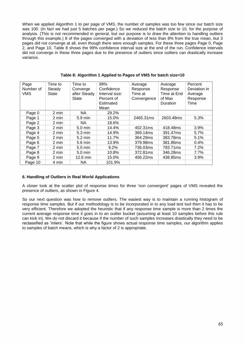
65

When we applied Algorithm 1 to per page of VMS, the number of samples was too few since our batch size was 100. (In fact we had just 5 batches per page.) So we reduced the batch size to 10, for the purpose of analysis. (This is not recommended in general, but our purpose is to draw the attention to handling outliers through this example.) 8 of the pages converged with a deviation of less than 8% from the true mean, but 3 pages did not converge at all, even though there were enough samples. For these three pages Page 0, Page 2, and Page 10, Table 8 shows the 99% confidence interval size at the end of the run. Confidence intervals did not converge in these three pages due to the presence of outliers since outliers can drastically increase variance.

Table 8: Algorithm 1 Applied to Pages of VMS for batch size=10

Page Number of VMS

Time to Steady State

Time to Converge after Steady State

99% Confidence Interval size: Percent of Estimated Mean

Average Response Time at Convergence

Average Response Time at End of Max Duration

Percent Deviation in Average Response Time

Page 0 2 min NA 29.2%

Page 1 2 min 5.9 min 15.0% 2465.31ms 2603.48ms 5.3%

Page 2 2 min NA 18.6%

Page 3 2 min 5.0 min 14.4% 402.31ms 418.48ms 3.9%

Page 4 2 min 5.3 min 14.9% 369.14ms 391.47ms 5.7%

Page 5 2 min 5.2 min 11.7% 364.29ms 383.78ms 5.1%

Page 6 2 min 5.6 min 13.9% 379.98ms 381.86ms 0.4%

Page 7 2 min 5.0 min 9.2% 736.03ms 793.71ms 7.2%

Page 8 2 min 5.0 min 10.8% 372.81ms 346.28ms 7.7%

Page 9 2 min 12.6 min 15.0% 456.22ms 438.85ms 3.9%

Page 10 4 min NA 101.9%

6. Handling of Outliers in Real World Applications

A closer look at the scatter plot of response times for three 'non convergent' pages of VMS revealed the presence of outliers, as shown in Figure 4.

So our next question was how to remove outliers. The easiest way is to maintain a running histogram of response time samples. But if our methodology is to be incorporated in to any load test tool then it has to be very efficient. Therefore we adopted the heuristic that if any response time sample is more than 2 times the current average response time it goes in to an outlier bucket (assuming at least 10 samples before this rule can kick in). We do not discard it because if the number of such samples increases drastically they need to be reclassified as ‘inliers’. Note that while the figure shows actual response time samples, our algorithm applies to samples of batch means, which is why a factor of 2 is appropriate.

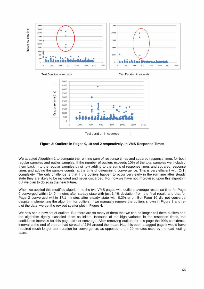
66

Figure 3: Outliers in Pages 0, 10 and 2 respectively, in VMS Response Times

We adapted Algorithm 1 to compute the running sum of response times and squared response times for both regular samples and outlier samples. If the number of outliers exceeds 10% of the total samples we included them back in to the regular samples by simply adding to the sums of response times and squared response times and adding the sample counts, at the time of determining convergence. This is very efficient with O(1) complexity. The only challenge is that if the outliers happen to occur very early in the run time after steady state they are likely to be included and never discarded. For now we have not improvised upon this algorithm but we plan to do so in the near future.

When we applied this modified algorithm to the two VMS pages with outliers, average response time for Page 0 converged within 14.9 minutes after steady state with just 1.4% deviation from the final result, and that for Page 2 converged within 17.1 minutes after steady state with 0.2% error. But Page 10 did not converge despite implementing the algorithm for outliers. If we manually remove the outliers shown in Figure 3 and re-plot the data, we get the revised scatter plot in Figure 4.

We now see a new set of outliers. But there are so many of them that we can no longer call them outliers and the algorithm rightly classified them as inliers. Because of the high variance in the response times, the confidence intervals for this page did not converge. After removing outliers for this page the 99% confidence interval at the end of the run had spread of 24% around the mean. Had this been a tagged page it would have required much longer test duration for convergence, as opposed to the 20 minutes used by the load testing team.

Test Duration in seconds Test Duration in seconds

Response tim

e (

ms)

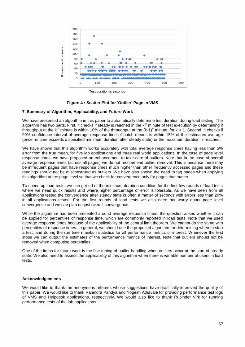
67

Figure 4 : Scatter Plot for 'Outlier' Page in VMS

7. Summary of Algorithm, Applicability, and Future Work

We have presented an algorithm in this paper to automatically determine test duration during load testing. The algorithm has two parts. First, it checks if steady is reached in the k

th minute of test execution by determining if

throughput at the kth minute is within 10% of the throughput at the (k-1)

st minute, for k > 1. Second, it checks if

99% confidence interval of average response time of batch means is within 15% of the estimated average (once runtime exceeds a specified minimum duration after steady state) or the maximum duration is reached.

We have shown that this algorithm works accurately with total average response times having less than 5% error from the true mean, for five lab applications and three real world applications. In the case of page level response times, we have proposed an enhancement to take care of outliers. Note that in the case of overall average response times (across all pages) we do not recommend outlier removal. This is because there may be infrequent pages that have response times much higher than other frequently accessed pages and these readings should not be misconstrued as outliers. We have also shown the need to tag pages when applying this algorithm at the page level so that we check for convergence only for pages that matter.

To speed up load tests, we can get rid of the minimum duration condition for the first few rounds of load tests where we need quick results and where higher percentage of error is tolerable. As we have seen from all applications tested the convergence after steady state is often a matter of seconds with errors less than 20% in all applications tested. For the first rounds of load tests we also need not worry about page level convergence and we can plan on just overall convergence.

While the algorithm has been presented around average response times, the question arises whether it can be applied for percentiles of response time, which are commonly reported in load tests. Note that we used average response times because of the applicability of the central limit theorem. We cannot do the same with percentiles of response times. In general, we should use the proposed algorithm for determining when to stop a test, and during the run time maintain statistics for all performance metrics of interest. Whenever the test stops we can output the estimates of the performance metrics of interest. Note that outliers should not be removed when computing percentiles.

One of the items for future work is the fine tuning of outlier handling when outliers occur at the start of steady state. We also need to assess the applicability of this algorithm when there is variable number of users in load tests.

Acknowledgements

We would like to thank the anonymous referees whose suggestions have drastically improved the quality of this paper. We would like to thank Rajendra Pandya and Yogesh Athavale for providing performance test logs of VMS and Helpdesk applications, respectively. We would also like to thank Rupinder Virk for running performance tests of the lab applications.

Test duration is seconds

Response tim

e (

ms)

68

References

[AUTOC] http://easycalculation.com/statistics/autocorrelation.php

[DELLDVD] Dell DVD Store http://linux.dell.com/dvdstore/

[EICK2007] M. Eickhoff, D. McNickle, K. Pawlikowski, ”Detecting the duration of initial transient in steady state simulation of arbitrary performance measures”, ValueTools(2007).

[FISH2001] G. Fishman, Discrete Event Simulation: Modelling, Programming, and Analysis, Springer (2001).

[JPET] iBatis jPetStore http://sourceforge.net/projects/ibatisjpetstore/

[PAWL1990] K. Pawlikowski,”Steady-state simulation of queuing processes: a survey of problems and solutions.”, ACM Computing Surveys, 22:123–170(1990).

[ROBI2007] S. Robinson,”A statistical process control approach to selecting a warm-up period for a discrete-event simulation.”, European Journal of Operational Research, 176(1):332–346(2007).

[RUBIS] Rice University Bidding System http://rubis.ow2.org/

[MANS2010] R. Mansharamani, A. Khanapurkar, B. Mathew, R. Subramanyan, "Performance Testing:

Far from Steady State", IEEE COMPSAC, 341-346(2010).

[TDIST] http://easycalculation.com/statistics/t-distribution-critical-value-table.php

[WALP2002] R. Walpole. Probability & Statistics for Engineers & Scientists. 7th Edition, Pearson (2002).

[WARMUP] http://rwwescott.wordpress.com/2014/07/29/when-does-the-warmup-end/

The copyright of this paper is owned by the author(s). The author(s) hereby grants Computer Measurement Group Inc a royalty free right to publish this paper in CMG India Annual Conference Proceedings.

69

Measuring Wait and Service Times in Java using Bytecode Instrumentation

Amol Khanapurkar, Chetan Phalak Tata Consultancy Services, Mumbai.

{amol.khanapurkar, chetan1.phalak}@tcs.com

Performance measurement is key to many performance engineering activities. Today's programs are invariably concurrent programs that try to optimize usage of resources such as multi-core and power. Concurrent programs are typically implemented using some sort of Queuing mechanism. Two key metrics in queuing architecture are Wait Time and Service Time. Preciseness of these two metrics determines how accurately and reliably the IT systems can be modeled. Queues are amply studied and rich literature is available, however there is paucity of tools available that provide a breakup of Wait Time and Service Time components of Response Time. In this paper, we demonstrate a technique that can be used for measuring the actual time spent in servicing the Synchronized block as well as time spent in waiting to enter the Synchronized block. A critical-section is implemented in Java using Synchronized blocks.

1. INTRODUCTION

Java programming language is one of the most widely adopted programming languages in the world today. It is present in all kinds of applications viz. Large Enterprises, Small and Medium businesses as well as in Mobile apps. One of the features that has made Java so popular is the built-in support for multi-threading to write concurrent and parallel programs. Vast majority of today’s enterprise applications written in Java are concurrent programs. By concurrent programs, we mean programs that exchange information through primitives provided by the native programming language. In Java, such a primitive is provided by the keyword ‘synchronized’. The Java infrastructure for providing concurrency support revolves around this keyword.

Concurrent programs in java are written using JDK API that support multi-threading. When two or more threads in Java try to enter a critical-section, Java enforces queuing so that only one thread can get a lock on critical-section. Upon completing its work the thread relinquishes the lock and leaves the critical-section. Remaining threads competing for the lock wait to acquire the lock. The Java runtime through its synchronization primitives manages the assignment of lock to the next eligible thread. Java offers support for queuing policies to be fair or random. Fair assignment is performance intensive and is rarely used in real life applications. Random assignment of the lock has no performance overheads and is hence preferred in most applications. Queuing is a vastly studied topic. Queuing theory [ QUAN 1984 ] provides the base for analytical modeling. Hence it is highly desirable to be able to apply queuing theory fundamentals on the actual code. Amongst other things, Queuing theory requires Service Time and Arrival rate as input parameters to be able to predict Wait Times and Response Times for jobs to complete. In practice though, it is easy to measure response time, but exact service time and hence wait times remain a little elusive to be measured. There simply aren’t enough tools available which provide queue depth or breakup of response time into service and wait time components.

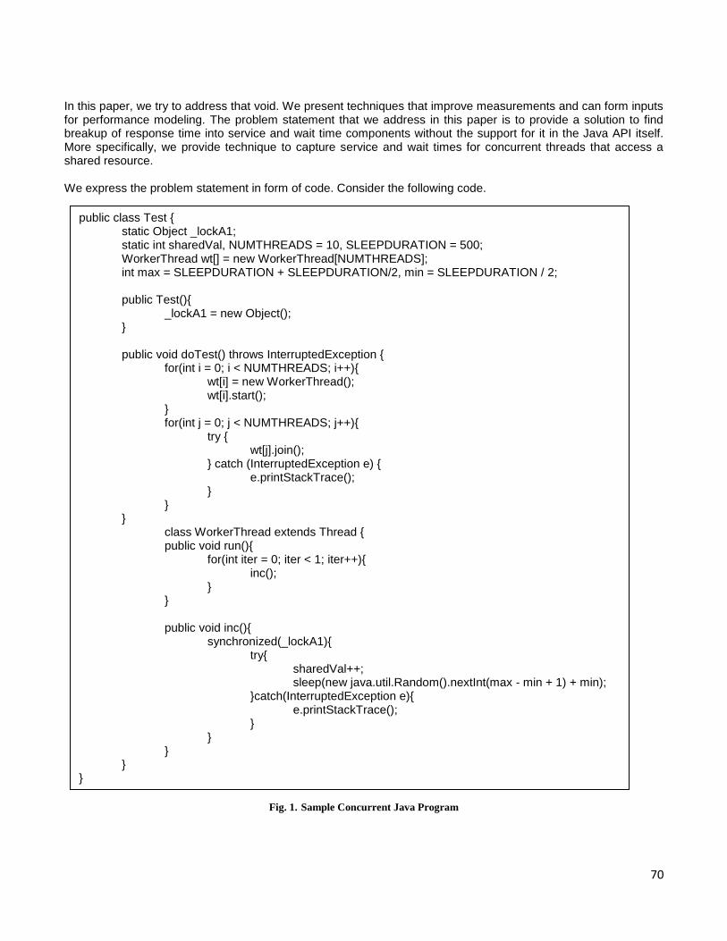
70

In this paper, we try to address that void. We present techniques that improve measurements and can form inputs for performance modeling. The problem statement that we address in this paper is to provide a solution to find breakup of response time into service and wait time components without the support for it in the Java API itself. More specifically, we provide technique to capture service and wait times for concurrent threads that access a shared resource. We express the problem statement in form of code. Consider the following code.

Fig. 1. Sample Concurrent Java Program

public class Test { static Object _lockA1; static int sharedVal, NUMTHREADS = 10, SLEEPDURATION = 500; WorkerThread wt[] = new WorkerThread[NUMTHREADS]; int max = SLEEPDURATION + SLEEPDURATION/2, min = SLEEPDURATION / 2; public Test(){ _lockA1 = new Object(); } public void doTest() throws InterruptedException { for(int i = 0; i < NUMTHREADS; i++){ wt[i] = new WorkerThread(); wt[i].start(); } for(int j = 0; j < NUMTHREADS; j++){ try { wt[j].join(); } catch (InterruptedException e) { e.printStackTrace(); } } } class WorkerThread extends Thread { public void run(){ for(int iter = 0; iter < 1; iter++){ inc(); } } public void inc(){ synchronized(_lockA1){ try{ sharedVal++; sleep(new java.util.Random().nextInt(max - min + 1) + min); }catch(InterruptedException e){ e.printStackTrace(); } } } } }

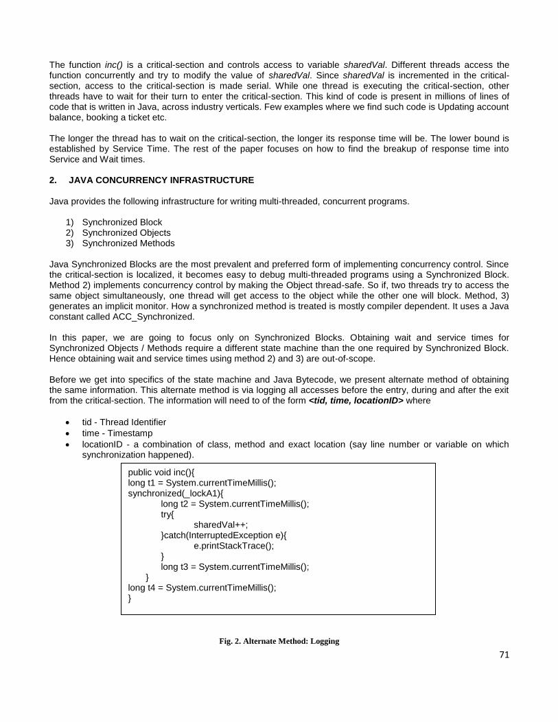
71

The function inc() is a critical-section and controls access to variable sharedVal. Different threads access the function concurrently and try to modify the value of sharedVal. Since sharedVal is incremented in the critical-section, access to the critical-section is made serial. While one thread is executing the critical-section, other threads have to wait for their turn to enter the critical-section. This kind of code is present in millions of lines of code that is written in Java, across industry verticals. Few examples where we find such code is Updating account balance, booking a ticket etc. The longer the thread has to wait on the critical-section, the longer its response time will be. The lower bound is established by Service Time. The rest of the paper focuses on how to find the breakup of response time into Service and Wait times. 2. JAVA CONCURRENCY INFRASTRUCTURE Java provides the following infrastructure for writing multi-threaded, concurrent programs.

1) Synchronized Block 2) Synchronized Objects 3) Synchronized Methods

Java Synchronized Blocks are the most prevalent and preferred form of implementing concurrency control. Since the critical-section is localized, it becomes easy to debug multi-threaded programs using a Synchronized Block. Method 2) implements concurrency control by making the Object thread-safe. So if, two threads try to access the same object simultaneously, one thread will get access to the object while the other one will block. Method, 3) generates an implicit monitor. How a synchronized method is treated is mostly compiler dependent. It uses a Java constant called ACC_Synchronized. In this paper, we are going to focus only on Synchronized Blocks. Obtaining wait and service times for Synchronized Objects / Methods require a different state machine than the one required by Synchronized Block. Hence obtaining wait and service times using method 2) and 3) are out-of-scope. Before we get into specifics of the state machine and Java Bytecode, we present alternate method of obtaining the same information. This alternate method is via logging all accesses before the entry, during and after the exit from the critical-section. The information will need to of the form <tid, time, locationID> where

tid - Thread Identifier

time - Timestamp

locationID - a combination of class, method and exact location (say line number or variable on which synchronization happened).

Fig. 2. Alternate Method: Logging

public void inc(){ long t1 = System.currentTimeMillis(); synchronized(_lockA1){

long t2 = System.currentTimeMillis(); try{ sharedVal++; }catch(InterruptedException e){ e.printStackTrace(); } long t3 = System.currentTimeMillis(); } long t4 = System.currentTimeMillis(); }

72

For each such access, there will need to be 4 tuples that need to get captured as shown below T1 – Time thread arrived at synchronized block. T2 – Time thread entered into synchronized block. T3 – Time, thread is about to exit synchronized block. T4 - Time thread exited synchronized block. In this case,

(T4 - T1) is the Response Time,

(T3 - T2) is the Service Time and

(T2 - T1) is the Wait Time. This method has the following disadvantages

1) Logging has its own overheads 2) After the logs have been written to, these logs will need to be crunched programmatically to get the

desired information 3) Even for simple programs, the crunching program can get complex because it has to tag the appropriate

timestamps to appropriate threads 4) For complex programs involving nested synchronized blocks (e.g. code that implements 2-phase

commits), the crunching program can quickly become more complex and mat require significant development and testing time

5) This method will fail in cases where source code is not available To overcome, these disadvantages we chose to implement bytecode instrumentation to capture the information we require. 3. JAVA BYTECODE Wikipedia [ BYTECODE ] defines Java bytecode as a list of the instructions that make up the Java bytecode, an abstract machine language that is ultimately executed by the Java virtual machine. The Java bytecode is generated by language compilers targeting the Java Platform, most notably the Java programming language. Synchronized Blocks are supported in the language using the bytecode instructions monitorenter and monitorexit. Monitorenter grabs the lock on the synchronized() section and monitorexit releases the same. 4. CENTRAL IDEA AND IMPLEMENTATION OF STATE MACHINE 4.1 Central Idea Our objective in building a state machine is to get the following details about a Synchronized Block.

Location of the block i.e. which class and which method is synchronized()

Variable name on which this block is synchronized()

Breakup of synchronized() block response time into wait and service time components Ingredients for implementing a critical-section using synchronized blocks are:

1) The synchronized() construct and 2) The variable on which synchronization is happening, either static or non-static

monitorenter and monitorexit opcodes provide events related to entering and exiting the critical-section. To get access to the variable name we need to track the opcodes getstatic and getfield for tracking static and non-static variables, respectively. Ideally tracking these 4 opcodes should suffice. This is the central idea behind the state machine. However we decided to add tracking of another opcode viz. astore to make the state machine more robust. We took this path for two reasons viz.

1) Typically, the javac compiler generates a bunch of opcodes between the get* and monitorenter opcode.

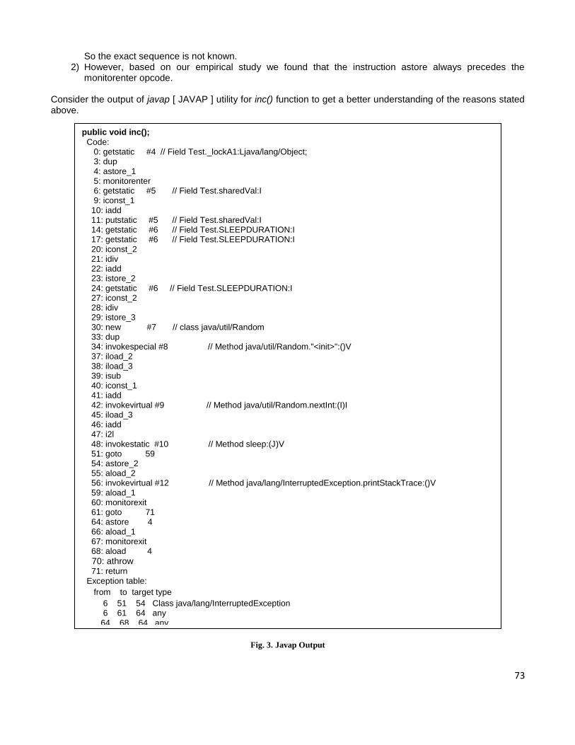
73

So the exact sequence is not known. 2) However, based on our empirical study we found that the instruction astore always precedes the

monitorenter opcode. Consider the output of javap [ JAVAP ] utility for inc() function to get a better understanding of the reasons stated above.

Fig. 3. Javap Output

public void inc();

Code: 0: getstatic #4 // Field Test._lockA1:Ljava/lang/Object; 3: dup 4: astore_1 5: monitorenter 6: getstatic #5 // Field Test.sharedVal:I 9: iconst_1 10: iadd 11: putstatic #5 // Field Test.sharedVal:I 14: getstatic #6 // Field Test.SLEEPDURATION:I 17: getstatic #6 // Field Test.SLEEPDURATION:I 20: iconst_2 21: idiv 22: iadd 23: istore_2 24: getstatic #6 // Field Test.SLEEPDURATION:I 27: iconst_2 28: idiv 29: istore_3 30: new #7 // class java/util/Random 33: dup 34: invokespecial #8 // Method java/util/Random."<init>":()V 37: iload_2 38: iload_3 39: isub 40: iconst_1 41: iadd 42: invokevirtual #9 // Method java/util/Random.nextInt:(I)I 45: iload_3 46: iadd 47: i2l 48: invokestatic #10 // Method sleep:(J)V 51: goto 59 54: astore_2 55: aload_2 56: invokevirtual #12 // Method java/lang/InterruptedException.printStackTrace:()V 59: aload_1 60: monitorexit 61: goto 71 64: astore 4 66: aload_1 67: monitorexit 68: aload 4

70: athrow 71: return Exception table:

from to target type

6 51 54 Class java/lang/InterruptedException 6 61 64 any 64 68 64 any

74

Notice the presence of dup and astore instructions (ignore everything starting from '_' character) between the getstatic and monitorenter opcodes. For various test programs written in various different ways and compiled with and without -O options, we found that the set of instructions were not the same. Had these instructions been the same always, we would be in a position to provide guarantee regarding the sequence of events leading to entering the critical-section. However, we found that astore opcode always precedes the monitorenter event. Hence, we made it a part of our pipeline of instructions to keep track of, to detect the presence of thread which is about to enter a critical-section. The monitorexit opcode is fairly straight forward. Upon encountering monitorexit, we just have to flush our data structures that keep track of the pipeline. In our study of Java literature, we haven't come across literature that gives strong guarantees regarding sequence of bytecode generation. Hence our implementation is empirical, based on our understanding of how the Java concurrency implementation infrastructure works. Since the implementation is based on empirical data, we carried out exhaustive testing which we will describe later in the paper. We didn't find any test case for which our state machine breaks. 4.2 Implementation We used the ASM [ ASM ] Bytecode Manipulation library to do the instrumentation. ASM is based on Visitor pattern. The ASM library generates events which are captured and processed by our own Java code. For ASM library to generate events we needed to register hooks for events of interest that were useful for us in implementing the state machine. The registering of hooks can be statically done at compile time or done at runtime i.e. at class load time using the Instrumentation API available since JDK 1.5. Since we anticipated this utility to be small (< 5K LOC), we preferred the static approach in which instrumentation is done manually. Conversion to runtime instrumentation is trivial and is just a matter of using the right APIs provided by Java. The ASM API provides the following hooks for events (of interest to us) to be generated

visitInsn() :- For monitorenter and monitorexit

visitVarInsn() :- For astore

visitFieldInsn() :- For getstatic and getfield

visitMethodInsn() :- For class and method names

During instrumentation the ASM implementation parses Java bytecode of classes. After parsing those classes, it generates events for which there is a hook registered. Once an event is generated, it is the responsibility of the calling code to consume the event. For performance reasons we use the streaming API of ASM. With streaming API an event is lost if it is not consumed. When an event is generated, the control returns to our calling code which needs to consume the event. The calling code takes appropriate actions based on the type {visitInsn, visitVarInsn, visitFieldInsn and visitMethodInsn} of the event generated. These events are encapsulated in two Visitors that need to work in lock-steps to be able to distinguish between a thread has arrive and when the thread has entered the monitor. These Visitors are named as

ResponseTimeMethodVisitor and

ServiceTimeMethodVisitor The algorithm that the ResponseTimeMethodVisitor implements is as follows

a) Maintain a list of opcodes in the order in which they are called. b) Obviously, we expect the getfield / getstatic as the first element in our list of opcodes. Maintain that at the

head of our list. Keep track of the latest getfield / getstatic opcodes, overwriting previous occurrences, if any.

c) Ignore all other events, if any are registered e.g. dup, until an astore is received. Add astore as second element of our list.

d) Ignore all other events, if any are registered until an astore or getfield / getstatic is received. e) If astore is received, overwrite it at second position in the list.

75

f) If getfield / getstatic is received, empty the list and add getfield / getstatic to the head of the list. g) Continue the same until first two elements are getfield / getstatic and astore respectively and the third

element is monitorenter. h) Once the list comprises of

1. getfield / getstatic 2. astore 3. monitorenter in that order, it sets the flag for that thread to true.

i) Once it sets the flag to true, it does update the book-keeping data structures. In one of the data structures, it sets the arrival time (T1) of current thread against the synchronized block implemented on variable pointed to by getfield / getstatic

j) Upon encountering a monitorexit event, it updates the book-keeping data structures by entering the time (T4) at which thread exited the synchronized block.

The ServiceTimeMethodVisitor simply piggybacks on the work that ResponseTimeMethodVisitor. It only does things mentioned below

a) Looks for the status of the flag that ResponseTimeMethodVisitor has set to true for current thread. Once it finds the flag to be set, it updates the book-keeping data structure by setting the syncblock enter time (T2) against the current thread. Updating the data-structure for a thread whose arrival time is not set before by ResponseTimeMethodVisitor is an illegal state.

b) After updating the data structure, it again resets the flag to false, so that nested synchronized blocks can be processed.

c) Since book-keeping data structures are common to both Visitors, it simply ignores the monitorexit event and treats time set by ResponseTimeMethodVisitor as the timestamp (T3) at which servicing is completed.

Thus in our state machine implementation

T3 and T4 are same

(T3 – T2) gives us the Service Time

(T4 – T1) gives us the Response Time The above description is for the simplest case. For nested synchronized blocks, the state machine gets a little more complex. Technically, however the same algorithm is followed since the methods in our Java code which maintains the state machine are reentrant. Only, the book-keeping and hence the results printing that get a little trickier to handle. 4.2 Output of State-machine For code snippet depicted in Fig. 1, assume appropriate main() is called. Our state machine then outputs the result in the following format

ThreadName ArrivalTime EnterTime ExitTime serviceTime waitTime LockName LockLocation

Thread-0 1408309576179 1408309576179 1408309576196 17 0 Test._lockA1 Test$WorkerThread.inc

Thread-1 1408309576205 1408309576205 1408309576221 16 0 Test._lockA1 Test$WorkerThread.inc

Thread-2 1408309576221 1408309576221 1408309576238 17 0 Test._lockA1 Test$WorkerThread.inc

Thread-3 1408309576238 1408309576239 1408309576264 25 1 Test._lockA1 Test$WorkerThread.inc

Thread-6 1408309576243 1408309576334 1408309576352 18 91 Test._lockA1 Test$WorkerThread.inc

Thread-4 1408309576243 1408309576352 1408309576369 17 109 Test._lockA1 Test$WorkerThread.inc

Thread-8 1408309576244 1408309576319 1408309576334 15 75 Test._lockA1 Test$WorkerThread.inc

Thread-5 1408309576245 1408309576302 1408309576319 17 57 Test._lockA1 Test$WorkerThread.inc

Thread-9 1408309576245 1408309576264 1408309576281 17 19 Test._lockA1 Test$WorkerThread.inc

Thread-7 1408309576245 1408309576281 1408309576301 20 36 Test._lockA1 Test$WorkerThread.inc

Fig. 4 Output from State-machine

76

5. TESTING STATE MACHINE IMPLEMENTATION The testing was divided into two types, viz.

1) Theory-based programs which demonstrate computer science principles or concepts

Producer-Consumer problem [ PRODCONS ]

Dining Philosopher problem [ DINIPHIL ]

Cigarette Smokers problem [ CIGARETTE ]

M/M/1 Queues [ MM1 ] In computing, the producer–consumer problem, dining philosopher problem and cigarette smokers problem are classic example of a multi- process synchronization problem. We implement these problems using JAVA. Each of these problem’s solutions, we design by creating common, fixed-size buffer used as a queue, which was shared among all participants. By writing synchronized block, we gave access of shared queue to every participant. We test proposed state-machine implementation on these problems. We perceived 100% accurate results with respect to the service time, lock time for every thread running. 2) Custom programs which are comparable to code that gets written in IT industry today

Database connection pooling code

Update account balance for money transfer transaction (2-phase commit) These programs check the qualitative and quantitative correctness of the code that passes through the state machine. Other than M/M/1 Queues all others verify the functional correctness of the state machine, while M/M/1 (which is actually a set of programs) validates the quantitative correctness. 6. APPLICATION OF STATE MACHINE TECHNIQUE Once response time is accurately broken down into wait and service time components, performance modeling becomes accurate. Other researchers have built utilities on top of our API to predict performance in the presence of software and hardware resource bottlenecks [ SUBH 2014 ].

1.

This technique once tool-ified can help in detecting performance bottlenecks. During development phases of Software Development Life Cycle (SDLC) this tool can provide immense value in troubleshooting performance issues. We haven’t quantified the performance overhead of our technique yet, but we believe it to be very low. Our basis for this assumption is our own past work in developing a java profiler, named Jensor [ AMOL 2011 ] using bytecode instrumentation techniques. 7. CONCLUSION It is possible to derive Wait and Service Time components of Response Times of concurrent programs written in Java using bytecode instrumentation techniques. Our state-machine based approach is capable of capturing these metrics which can be used for other performance engineering activities like performance modeling, capacity planning and during performance testing.

77

REFERENCES

[ AMOL 2011 ] Amol Khanapurkar, Suresh Malan “Performance Engineering of a Java Profiler”, NCISE, Feb – 2011.[ ASM ] http://asm.ow2.org/

[ BYTECODE ]http://en.wikipedia.org/wiki/Java_bytecode

[ CIGARETTE ] http://en.wikipedia.org/wiki/Cigarette_smokers_problem

[ DINIPHIL ] http://en.wikipedia.org/wiki/Dining_philosophers_problem

[ JAVAP ] http://docs.oracle.com/javase/7/docs/technotes/tools/windows/javap.html

[ MM1 ] http://en.wikipedia.org/wiki/M/M/1_queue

[ PRODCONS ] http://en.wikipedia.org/wiki/Producer%E2%80%93consumer_problem

[ QUAN 1984 ] Lazowska et al: Quantitative System : computer system analysis using queuing network models, A popular book, 1984

[ SUBH 2014 ] Subhasri Duttagupta, Rupinder Virk and Manoj Nambiar, "Predicting Performance in the Presence of Software and Hardware Resource Bottlenecks", SPECTS, 2014.

78

CLOUD PERFORMANCE TESTING - KEY CONSIDERATIONS (COMPLETE

ANALYSIS USING RETAIL APPLICATION TEST DATA)

Abhijeet Padwal

Performance engineering group

Persistent Systems, Pune

email: abhijeet_padwal@persistent.co.in

Due to its lower cost and greater flexibility, cloud has become the most preferred option for the deployments for

any size of the applications and products in today’s world. Through its Platform as a Service (PaaS) and

Infrastructure as a Service (IaaS) services, cloud has attracted and benefitted the testing services of the

applications especially the load and performance testing. Though cloud provides superior flexibility, scalability at

lower cost over the traditional on-premises deployments, it has got its own limitations and challenges. If those

limitations are not evaluated carefully they can severely impact overall projects and their budgets if not evaluated

carefully. It is recommended to take holistic view while deciding about using cloud for any purpose by taking

detailed look at pros and cons of cloud.

This paper illustrate cloud in brief and a detail case study a load testing of a Retail application in cloud and how

cloud’s pros and cons worked in favor and against during the course of load testing and what actions needed to

be taken to overcome those.

The copyright of this paper is owned by the author(s). The author(s) hereby grants Computer Measurement Group Inc a royalty free right to publish this paper in CMG India Annual Conference Proceedings.

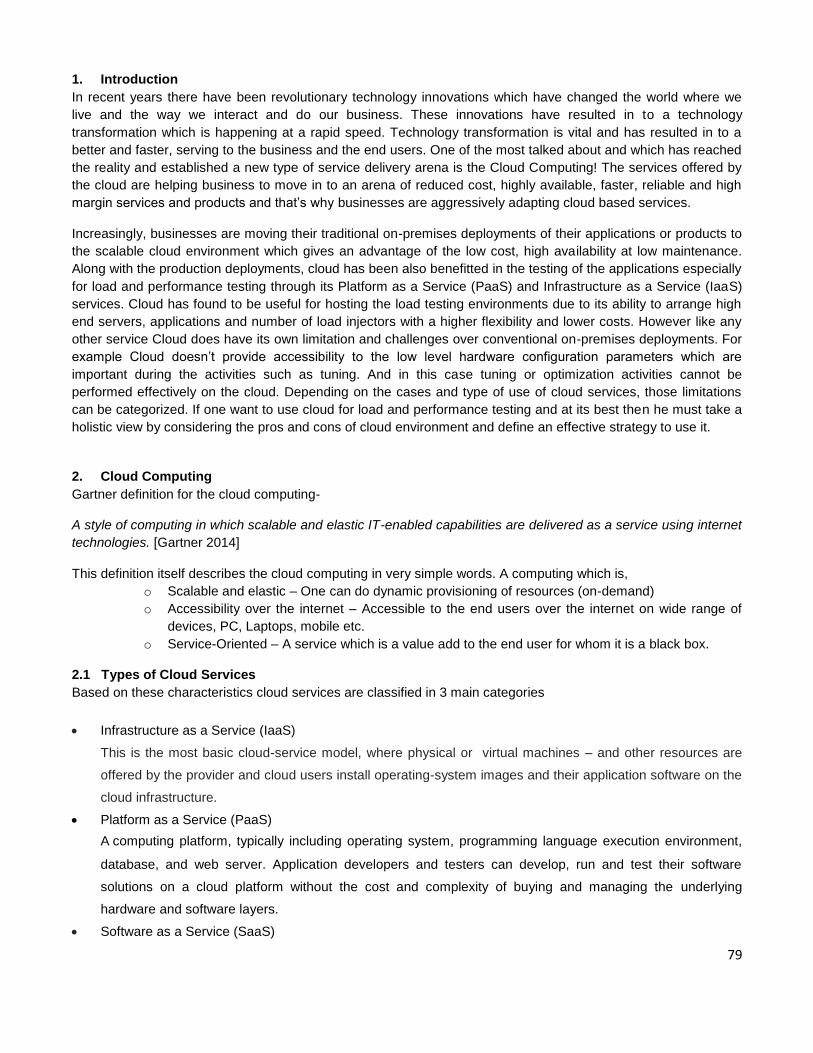
79

1. Introduction

In recent years there have been revolutionary technology innovations which have changed the world where we

live and the way we interact and do our business. These innovations have resulted in to a technology

transformation which is happening at a rapid speed. Technology transformation is vital and has resulted in to a

better and faster, serving to the business and the end users. One of the most talked about and which has reached

the reality and established a new type of service delivery arena is the Cloud Computing! The services offered by

the cloud are helping business to move in to an arena of reduced cost, highly available, faster, reliable and high

margin services and products and that’s why businesses are aggressively adapting cloud based services.

Increasingly, businesses are moving their traditional on-premises deployments of their applications or products to

the scalable cloud environment which gives an advantage of the low cost, high availability at low maintenance.

Along with the production deployments, cloud has been also benefitted in the testing of the applications especially

for load and performance testing through its Platform as a Service (PaaS) and Infrastructure as a Service (IaaS)

services. Cloud has found to be useful for hosting the load testing environments due to its ability to arrange high

end servers, applications and number of load injectors with a higher flexibility and lower costs. However like any

other service Cloud does have its own limitation and challenges over conventional on-premises deployments. For

example Cloud doesn’t provide accessibility to the low level hardware configuration parameters which are

important during the activities such as tuning. And in this case tuning or optimization activities cannot be

performed effectively on the cloud. Depending on the cases and type of use of cloud services, those limitations

can be categorized. If one want to use cloud for load and performance testing and at its best then he must take a

holistic view by considering the pros and cons of cloud environment and define an effective strategy to use it.

2. Cloud Computing

Gartner definition for the cloud computing-

A style of computing in which scalable and elastic IT-enabled capabilities are delivered as a service using internet

technologies. [Gartner 2014]

This definition itself describes the cloud computing in very simple words. A computing which is,

o Scalable and elastic – One can do dynamic provisioning of resources (on-demand)

o Accessibility over the internet – Accessible to the end users over the internet on wide range of

devices, PC, Laptops, mobile etc.

o Service-Oriented – A service which is a value add to the end user for whom it is a black box.

2.1 Types of Cloud Services

Based on these characteristics cloud services are classified in 3 main categories

Infrastructure as a Service (IaaS)

This is the most basic cloud-service model, where physical or virtual machines – and other resources are

offered by the provider and cloud users install operating-system images and their application software on the

cloud infrastructure.

Platform as a Service (PaaS)

A computing platform, typically including operating system, programming language execution environment,

database, and web server. Application developers and testers can develop, run and test their software

solutions on a cloud platform without the cost and complexity of buying and managing the underlying

hardware and software layers.

Software as a Service (SaaS)

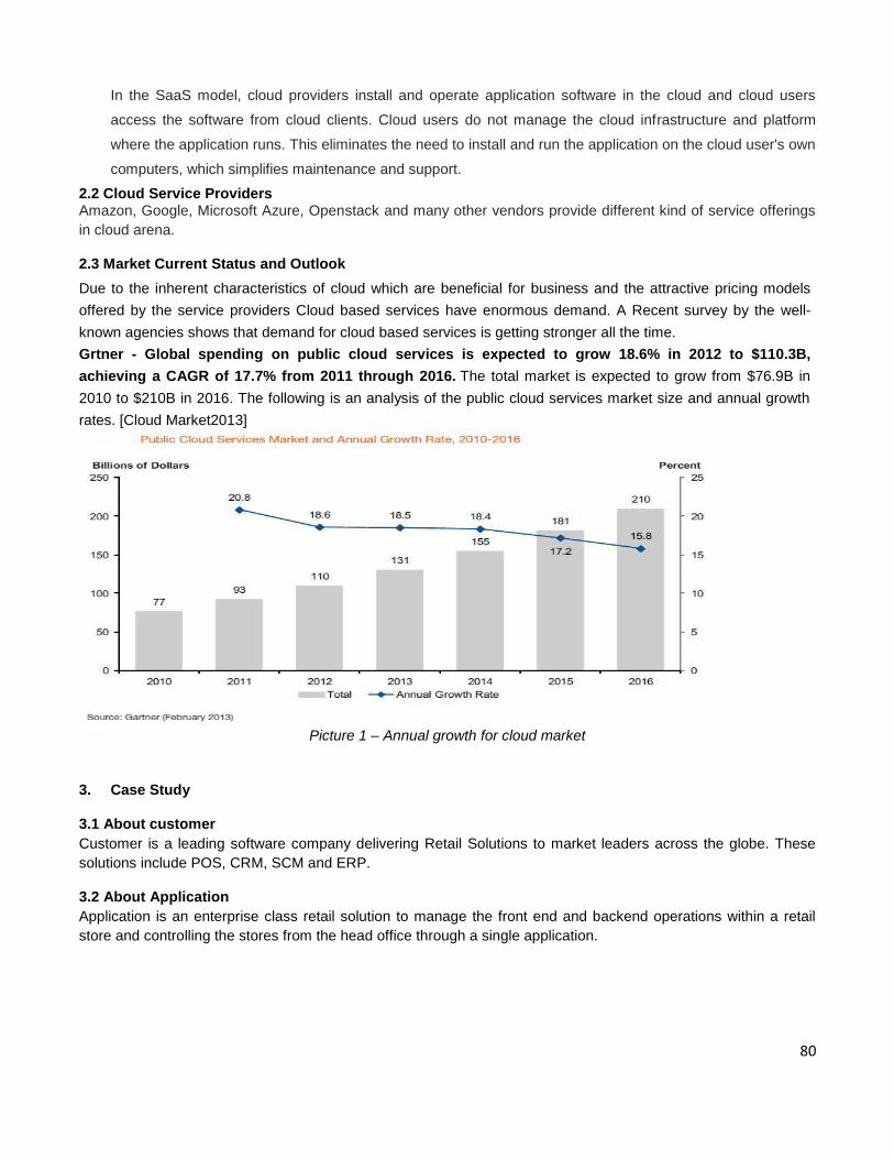
80

In the SaaS model, cloud providers install and operate application software in the cloud and cloud users

access the software from cloud clients. Cloud users do not manage the cloud infrastructure and platform

where the application runs. This eliminates the need to install and run the application on the cloud user's own

computers, which simplifies maintenance and support.

2.2 Cloud Service Providers Amazon, Google, Microsoft Azure, Openstack and many other vendors provide different kind of service offerings

in cloud arena.

2.3 Market Current Status and Outlook

Due to the inherent characteristics of cloud which are beneficial for business and the attractive pricing models

offered by the service providers Cloud based services have enormous demand. A Recent survey by the well-

known agencies shows that demand for cloud based services is getting stronger all the time.

Grtner - Global spending on public cloud services is expected to grow 18.6% in 2012 to $110.3B,

achieving a CAGR of 17.7% from 2011 through 2016. The total market is expected to grow from $76.9B in

2010 to $210B in 2016. The following is an analysis of the public cloud services market size and annual growth

rates. [Cloud Market2013]

Picture 1 – Annual growth for cloud market

3. Case Study

3.1 About customer

Customer is a leading software company delivering Retail Solutions to market leaders across the globe. These

solutions include POS, CRM, SCM and ERP.

3.2 About Application

Application is an enterprise class retail solution to manage the front end and backend operations within a retail

store and controlling the stores from the head office through a single application.

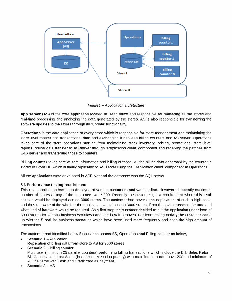
81

Figure1 – Application architecture

App server (AS) is the core application located at Head office and responsible for managing all the stores and

real-time processing and analyzing the data generated by the stores. AS is also responsible for transferring the

software updates to the stores through its ‘Update’ functionality.

Operations is the core application at every store which is responsible for store management and maintaining the

store level master and transactional data and exchanging it between billing counters and AS server. Operations

takes care of the store operations starting from maintaining stock inventory, pricing, promotions, store level

reports, online data transfer to AS server through ‘Replication client’ component and receiving the patches from

EAS server and transferring those to counters.

Billing counter takes care of item information and billing of those. All the billing data generated by the counter is

stored in Store DB which is finally replicated to AS server using the ‘Replication client’ component at Operations.

All the applications were developed in ASP.Net and the database was the SQL server.

3.3 Performance testing requirement

This retail application has been deployed at various customers and working fine. However till recently maximum

number of stores at any of the customers were 200. Recently the customer got a requirement where this retail

solution would be deployed across 3000 stores. The customer had never done deployment at such a high scale

and thus unaware of the whether the application would sustain 3000 stores, if not then what needs to be tune and

what kind of hardware would be required. As a first step the customer decided to put the application under load of

3000 stores for various business workflows and see how it behaves. For load testing activity the customer came

up with the 5 real life business scenarios which have been used more frequently and does the high amount of

transactions.

The customer had identified below 5 scenarios across AS, Operations and Billing counter as below,

Scenario 1 –Replication Replication of billing data from store to AS for 3000 stores.

Scenario 2 – Billing counter Multi user (minimum 25 parallel counters) performing billing transactions which include the Bill, Sales Return, Bill Cancellation, Lost Sales (in order of execution priority) with max line item not above 200 and minimum of 20 line items with Cash and Credit card as payment.

Scenario 3 – AS

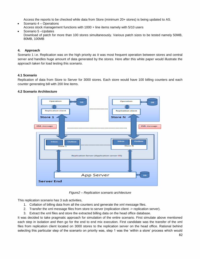
82

Access the reports to be checked while data from Store (minimum 20+ stores) is being updated to AS.

Scenario 4 – Operations Access stock management functions with 1000 + line items namely with 5/10 users

Scenario 5 –Updates Download of patch for more than 100 stores simultaneously. Various patch sizes to be tested namely 50MB, 80MB, 100MB

4. Approach

Scenario 1 i.e. Replication was on the high priority as it was most frequent operation between stores and central

server and handles huge amount of data generated by the stores. Here after this white paper would illustrate the

approach taken for load testing this scenario.

4.1 Scenario

Replication of data from Store to Server for 3000 stores. Each store would have 100 billing counters and each

counter generating bill with 200 line items.

4.2 Scenario Architecture

Figure2 – Replication scenario architecture

This replication scenario has 3 sub activities,

1. Collation of billing data from all the counters and generate the xml message files.

2. Transfer the xml message files from store to server (replication client -> replication server).

3. Extract the xml files and store the extracted billing data on the head office database.

It was decided to take pragmatic approach for simulation of the entire scenario. First simulate above mentioned

each step in isolation and then go for the end to end mix execution. First candidate was the transfer of the xml

files from replication client located on 3000 stores to the replication server on the head office. Rational behind

selecting this particular step of the scenario on priority was, step 1 was the ‘within a store’ process which would

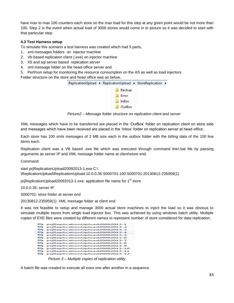
83

have max to max 100 counters each store so the max load for this step at any given point would be not more than

100. Step 2 is the event when actual load of 3000 stores would come in to picture so it was decided to start with

that particular step.

4.3 Test Harness setup

To simulate this scenario a test harness was created which had 5 parts,

1. xml messages folders on injector machine

2. Vb based replication client (.exe) on injector machine

3. IIS and sql server based replication server

4. xml message folder on the head-office server and

5. Perfmon setup for monitoring the resource consumption on the AS as well as load injectors.

Folder structure on the store and head office was as below,

Picture2 – Message folder structure on replication client and server

XML messages which have to be transferred are placed in the ‘OutBox’ folder on replication client on store side

and messages which have been received are placed in the ‘Inbox’ folder on replication server at head-office.

Each store has 100 xmls messages of 2 MB size each in the outbox folder with the billing data of the 100 line

items each.

Replication client was a VB based .exe file which was executed through command line\.bat file by passing

arguments as server IP and XML message folder name at client\store end.

Command:

start prjReplicationUpload20092013-1.exe C:\

\ReplicationUpload\ReplicationUpload:10.0.0.35:S000701:100:S000701:20130812-235959(1)

prjReplicationUpload20092013-1.exe: application file name for 1st store

10.0.0.35: server IP

S000701: store folder at server end

20130812-235959(1): XML message folder at client end

It was not feasible to setup and manage 3000 actual store machines to inject the load so it was obvious to

simulate multiple stores from single load injector box. This was achieved by using windows batch utility. Multiple

copies of EXE files were created by different names to represent number of store considered for data replication.

Picture 3 – Multiple copies of replication utility

A batch file was created to execute all exes one after another in a sequence.

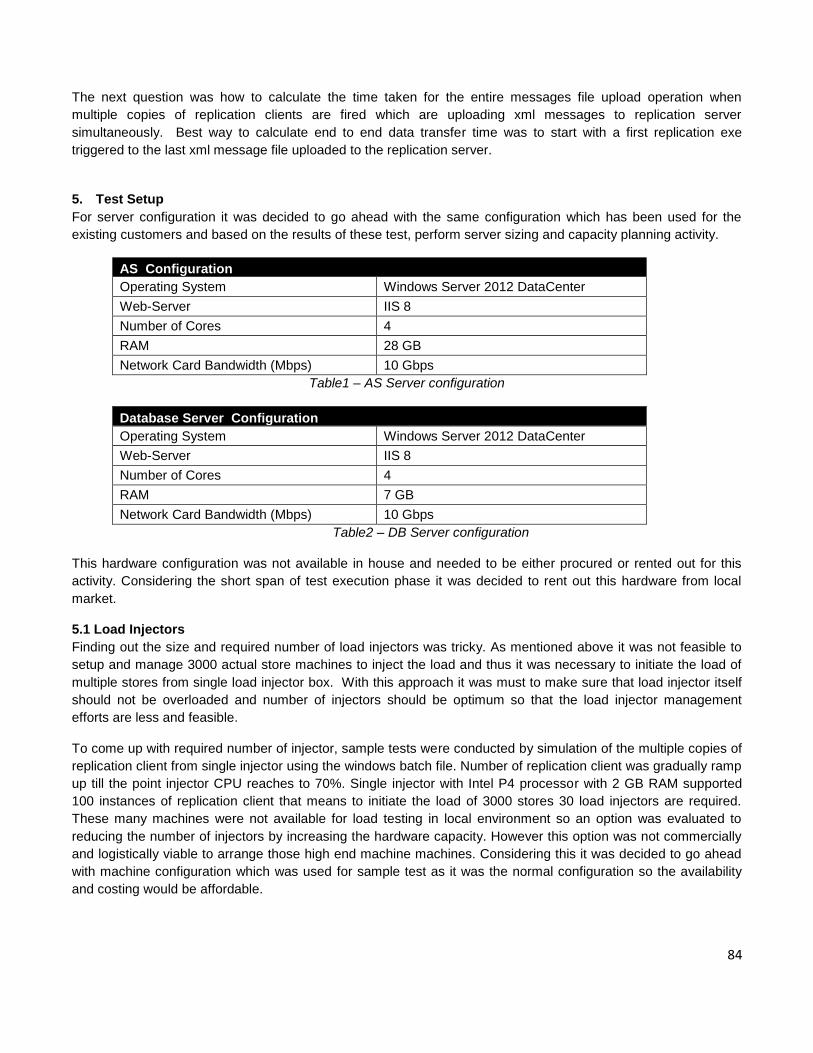
84

The next question was how to calculate the time taken for the entire messages file upload operation when

multiple copies of replication clients are fired which are uploading xml messages to replication server

simultaneously. Best way to calculate end to end data transfer time was to start with a first replication exe

triggered to the last xml message file uploaded to the replication server.

5. Test Setup

For server configuration it was decided to go ahead with the same configuration which has been used for the

existing customers and based on the results of these test, perform server sizing and capacity planning activity.

AS Configuration

Operating System Windows Server 2012 DataCenter

Web-Server IIS 8

Number of Cores 4

RAM 28 GB

Network Card Bandwidth (Mbps) 10 Gbps

Table1 – AS Server configuration

Database Server Configuration

Operating System Windows Server 2012 DataCenter

Web-Server IIS 8

Number of Cores 4

RAM 7 GB

Network Card Bandwidth (Mbps) 10 Gbps

Table2 – DB Server configuration

This hardware configuration was not available in house and needed to be either procured or rented out for this

activity. Considering the short span of test execution phase it was decided to rent out this hardware from local

market.

5.1 Load Injectors

Finding out the size and required number of load injectors was tricky. As mentioned above it was not feasible to

setup and manage 3000 actual store machines to inject the load and thus it was necessary to initiate the load of

multiple stores from single load injector box. With this approach it was must to make sure that load injector itself

should not be overloaded and number of injectors should be optimum so that the load injector management

efforts are less and feasible.

To come up with required number of injector, sample tests were conducted by simulation of the multiple copies of

replication client from single injector using the windows batch file. Number of replication client was gradually ramp

up till the point injector CPU reaches to 70%. Single injector with Intel P4 processor with 2 GB RAM supported

100 instances of replication client that means to initiate the load of 3000 stores 30 load injectors are required.

These many machines were not available for load testing in local environment so an option was evaluated to

reducing the number of injectors by increasing the hardware capacity. However this option was not commercially

and logistically viable to arrange those high end machine machines. Considering this it was decided to go ahead

with machine configuration which was used for sample test as it was the normal configuration so the availability

and costing would be affordable.

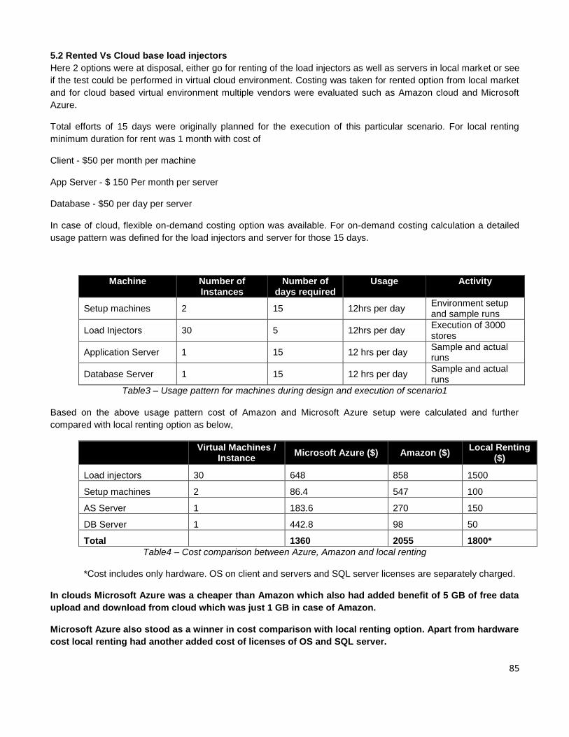
85

5.2 Rented Vs Cloud base load injectors

Here 2 options were at disposal, either go for renting of the load injectors as well as servers in local market or see

if the test could be performed in virtual cloud environment. Costing was taken for rented option from local market

and for cloud based virtual environment multiple vendors were evaluated such as Amazon cloud and Microsoft

Azure.

Total efforts of 15 days were originally planned for the execution of this particular scenario. For local renting

minimum duration for rent was 1 month with cost of

Client - $50 per month per machine

App Server - $ 150 Per month per server

Database - $50 per day per server

In case of cloud, flexible on-demand costing option was available. For on-demand costing calculation a detailed

usage pattern was defined for the load injectors and server for those 15 days.

Machine Number of Instances

Number of days required

Usage Activity

Setup machines 2 15 12hrs per day Environment setup and sample runs

Load Injectors 30 5 12hrs per day Execution of 3000 stores

Application Server 1 15 12 hrs per day Sample and actual runs

Database Server 1 15 12 hrs per day Sample and actual runs

Table3 – Usage pattern for machines during design and execution of scenario1

Based on the above usage pattern cost of Amazon and Microsoft Azure setup were calculated and further

compared with local renting option as below,

Virtual Machines /

Instance Microsoft Azure ($) Amazon ($)

Local Renting ($)

Load injectors 30 648 858 1500

Setup machines 2 86.4 547 100

AS Server 1 183.6 270 150

DB Server 1 442.8 98 50

Total 1360 2055 1800*

Table4 – Cost comparison between Azure, Amazon and local renting

*Cost includes only hardware. OS on client and servers and SQL server licenses are separately charged.

In clouds Microsoft Azure was a cheaper than Amazon which also had added benefit of 5 GB of free data

upload and download from cloud which was just 1 GB in case of Amazon.

Microsoft Azure also stood as a winner in cost comparison with local renting option. Apart from hardware

cost local renting had another added cost of licenses of OS and SQL server.

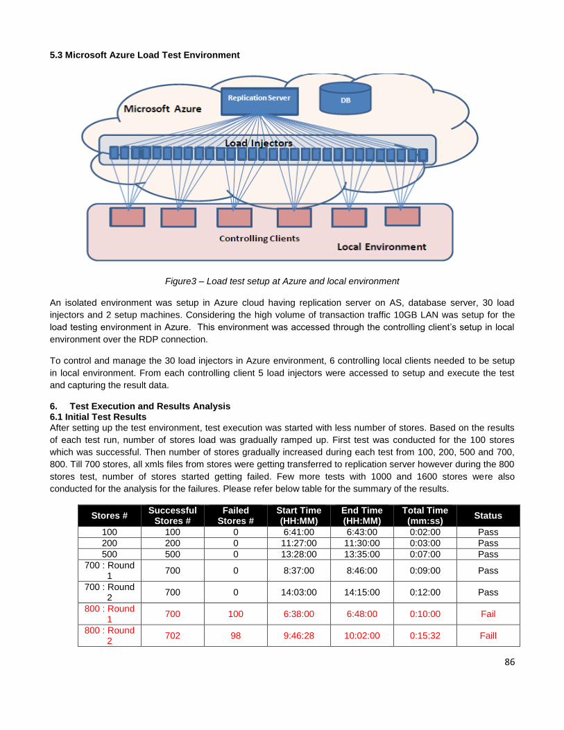
86

5.3 Microsoft Azure Load Test Environment

Figure3 – Load test setup at Azure and local environment

An isolated environment was setup in Azure cloud having replication server on AS, database server, 30 load

injectors and 2 setup machines. Considering the high volume of transaction traffic 10GB LAN was setup for the

load testing environment in Azure. This environment was accessed through the controlling client’s setup in local

environment over the RDP connection.

To control and manage the 30 load injectors in Azure environment, 6 controlling local clients needed to be setup

in local environment. From each controlling client 5 load injectors were accessed to setup and execute the test

and capturing the result data.

6. Test Execution and Results Analysis 6.1 Initial Test Results

After setting up the test environment, test execution was started with less number of stores. Based on the results

of each test run, number of stores load was gradually ramped up. First test was conducted for the 100 stores

which was successful. Then number of stores gradually increased during each test from 100, 200, 500 and 700,

800. Till 700 stores, all xmls files from stores were getting transferred to replication server however during the 800

stores test, number of stores started getting failed. Few more tests with 1000 and 1600 stores were also

conducted for the analysis for the failures. Please refer below table for the summary of the results.

Stores # Successful

Stores # Failed

Stores # Start Time (HH:MM)

End Time (HH:MM)

Total Time (mm:ss)

Status

100 100 0 6:41:00 6:43:00 0:02:00 Pass

200 200 0 11:27:00 11:30:00 0:03:00 Pass

500 500 0 13:28:00 13:35:00 0:07:00 Pass

700 : Round 1

700 0 8:37:00 8:46:00 0:09:00 Pass

700 : Round 2

700 0 14:03:00 14:15:00 0:12:00 Pass

800 : Round 1

700 100 6:38:00 6:48:00 0:10:00 Fail

800 : Round 2

702 98 9:46:28 10:02:00 0:15:32 Faill

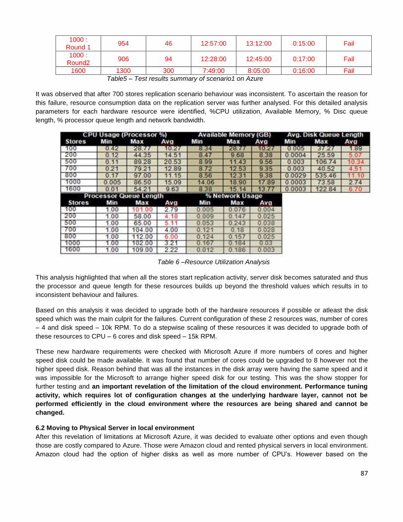
87

1000 : Round 1

954 46 12:57:00 13:12:00 0:15:00 Fail

1000 : Round2

906 94 12:28:00 12:45:00 0:17:00 Fail

1600 1300 300 7:49:00 8:05:00 0:16:00 Fail

Table5 – Test results summary of scenario1 on Azure

It was observed that after 700 stores replication scenario behaviour was inconsistent. To ascertain the reason for

this failure, resource consumption data on the replication server was further analysed. For this detailed analysis

parameters for each hardware resource were identified, %CPU utilization, Available Memory, % Disc queue

length, % processor queue length and network bandwidth.

Table 6 –Resource Utilization Analysis

This analysis highlighted that when all the stores start replication activity, server disk becomes saturated and thus

the processor and queue length for these resources builds up beyond the threshold values which results in to

inconsistent behaviour and failures.

Based on this analysis it was decided to upgrade both of the hardware resources if possible or atleast the disk

speed which was the main culprit for the failures. Current configuration of these 2 resources was, number of cores

– 4 and disk speed – 10k RPM. To do a stepwise scaling of these resources it was decided to upgrade both of

these resources to CPU – 6 cores and disk speed – 15k RPM.

These new hardware requirements were checked with Microsoft Azure if more numbers of cores and higher

speed disk could be made available. It was found that number of cores could be upgraded to 8 however not the

higher speed disk. Reason behind that was all the instances in the disk array were having the same speed and it

was impossible for the Microsoft to arrange higher speed disk for our testing. This was the show stopper for

further testing and an important revelation of the limitation of the cloud environment. Performance tuning

activity, which requires lot of configuration changes at the underlying hardware layer, cannot not be

performed efficiently in the cloud environment where the resources are being shared and cannot be

changed.

6.2 Moving to Physical Server in local environment

After this revelation of limitations at Microsoft Azure, it was decided to evaluate other options and even though

those are costly compared to Azure. Those were Amazon cloud and rented physical servers in local environment.

Amazon cloud had the option of higher disks as well as more number of CPU’s. However based on the

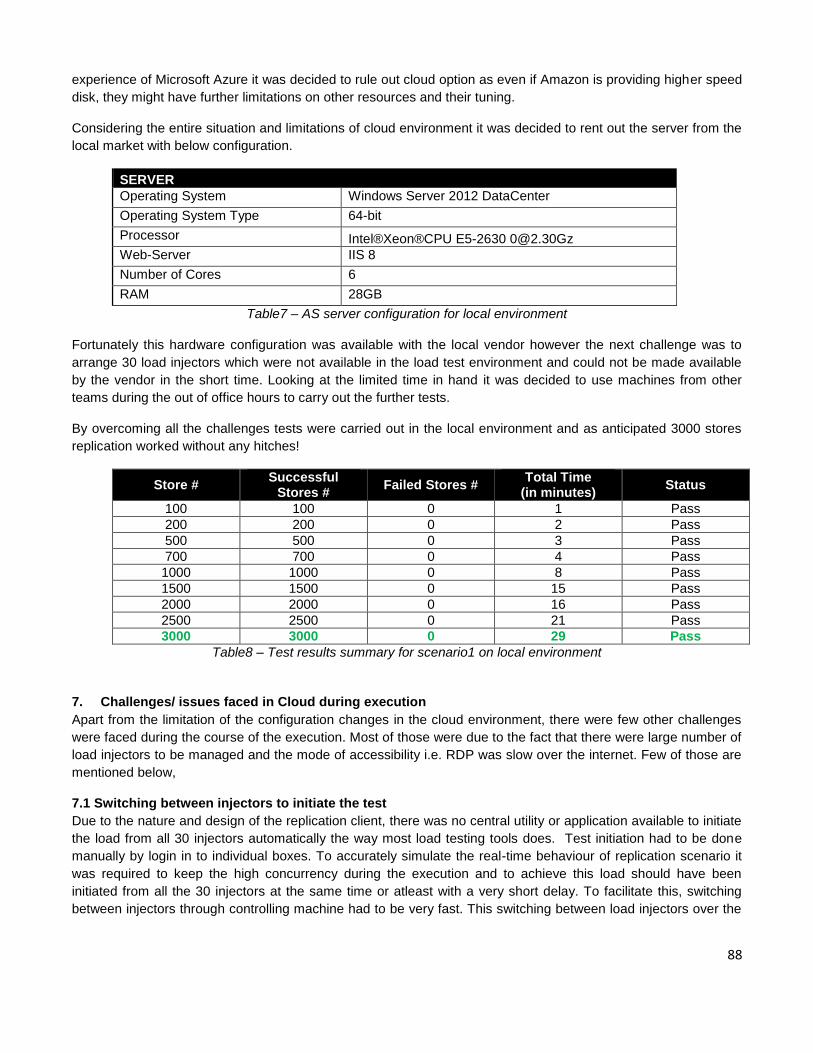
88

experience of Microsoft Azure it was decided to rule out cloud option as even if Amazon is providing higher speed

disk, they might have further limitations on other resources and their tuning.

Considering the entire situation and limitations of cloud environment it was decided to rent out the server from the

local market with below configuration.

SERVER

Operating System Windows Server 2012 DataCenter

Operating System Type 64-bit

Processor Intel®Xeon®CPU E5-2630 0@2.30Gz

Web-Server IIS 8

Number of Cores 6

RAM 28GB

Table7 – AS server configuration for local environment

Fortunately this hardware configuration was available with the local vendor however the next challenge was to

arrange 30 load injectors which were not available in the load test environment and could not be made available

by the vendor in the short time. Looking at the limited time in hand it was decided to use machines from other

teams during the out of office hours to carry out the further tests.

By overcoming all the challenges tests were carried out in the local environment and as anticipated 3000 stores

replication worked without any hitches!

Store # Successful

Stores # Failed Stores #

Total Time (in minutes)

Status

100 100 0 1 Pass

200 200 0 2 Pass

500 500 0 3 Pass

700 700 0 4 Pass

1000 1000 0 8 Pass

1500 1500 0 15 Pass

2000 2000 0 16 Pass

2500 2500 0 21 Pass

3000 3000 0 29 Pass

Table8 – Test results summary for scenario1 on local environment

7. Challenges/ issues faced in Cloud during execution

Apart from the limitation of the configuration changes in the cloud environment, there were few other challenges

were faced during the course of the execution. Most of those were due to the fact that there were large number of

load injectors to be managed and the mode of accessibility i.e. RDP was slow over the internet. Few of those are

mentioned below,

7.1 Switching between injectors to initiate the test

Due to the nature and design of the replication client, there was no central utility or application available to initiate

the load from all 30 injectors automatically the way most load testing tools does. Test initiation had to be done

manually by login in to individual boxes. To accurately simulate the real-time behaviour of replication scenario it

was required to keep the high concurrency during the execution and to achieve this load should have been

initiated from all the 30 injectors at the same time or atleast with a very short delay. To facilitate this, switching

between injectors through controlling machine had to be very fast. This switching between load injectors over the

89

RDP connectivity was tedious, it would have been very easy if there would have been 30 controller machines

each managing single injector but it was not the case in this particular scenario.

7.2 Test data setup

Test setup included various task and one of the difficult one was creating folder setup for the 100 stores per

injector. During each execution cycle it was required to use unique bill number for the billing data so the message

folders were required to be updated before each test cycle with unique bill number in each store folder. Setting up

folder structures on 30 client machines to simulate 3000 stores was tedious and time consuming task and

performing it over RDP had added more complexity and time to it.

7.3 Monitoring

It was also necessary to monitor the health of each load injector during the execution to make sure that those are

not overloaded. Keeping an eye on resource consumption of 5 load injectors from a single controlling machine

was challenging.

7,4 Data transfer

These tests generated huge amount of result data including the resource utilization data. In absence of the

applications such as Microsoft excel and slow speed of the RDP connectivity it was difficult to perform the

analysis of this data on cloud machines itself so that data had to be downloaded for every test run. Downloading

of large amount of data over the internet connection was a time consuming process and there were cost involved

after the stipulated limit set by Microsoft for data transfer.

8. Conclusion and outlook

For load and performance testing, cloud provides an edge over the conventional on-premises test setups. One

can take advantage of the cloud to build the test environments within a very short period of time with a cost and

logistical flexibility however with all these advantages there are few disadvantages or challenges with the cloud

environment which could severely hamper the purpose. A limitation such as no access to the underlying hardware

configuration parameters doesn’t suit for the activities such as bottleneck identification, tuning and optimization.

Managing cloud setup remotely and data transfer over internet adds few more complexities and delays in overall

schedule.

One can consider cloud for load and performance testing however it is recommended that all these pros and cons

should be studied in details and that too in the context of the load testing requirement, see what could be possible

and what cannot be performed on cloud and base on that define the strategy to perform load testing on cloud.

References

[Gartner 2014]– http://www.gartner.com/it-glossary/cloud-computing/

[Cloud market 2013 ]– Gartner survey

http://www.forbes.com/sites/louiscolumbus/2013/02/19/gartner-predicts-infrastructure-services-will-

accelerate-cloud-computing-growth/

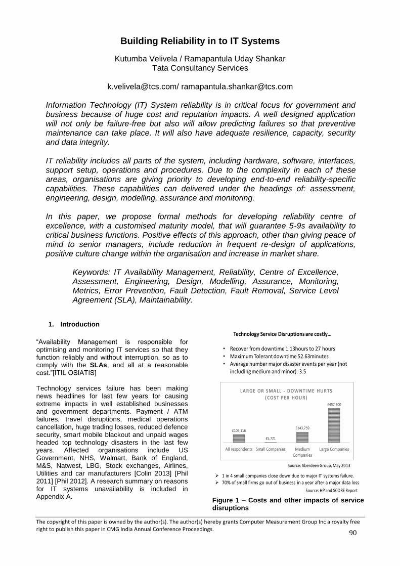
The copyright of this paper is owned by the author(s). The author(s) hereby grants Computer Measurement Group Inc a royalty free right to publish this paper in CMG India Annual Conference Proceedings.

90

Building Reliability in to IT Systems

Kutumba Velivela / Ramapantula Uday Shankar Tata Consultancy Services

k.velivela@tcs.com/ ramapantula.shankar@tcs.com

Information Technology (IT) System reliability is in critical focus for government and business because of huge cost and reputation impacts. A well designed application will not only be failure-free but also will allow predicting failures so that preventive maintenance can take place. It will also have adequate resilience, capacity, security and data integrity. IT reliability includes all parts of the system, including hardware, software, interfaces, support setup, operations and procedures. Due to the complexity in each of these areas, organisations are giving priority to developing end-to-end reliability-specific capabilities. These capabilities can delivered under the headings of: assessment, engineering, design, modelling, assurance and monitoring. In this paper, we propose formal methods for developing reliability centre of excellence, with a customised maturity model, that will guarantee 5-9s availability to critical business functions. Positive effects of this approach, other than giving peace of mind to senior managers, include reduction in frequent re-design of applications, positive culture change within the organisation and increase in market share.

Keywords: IT Availability Management, Reliability, Centre of Excellence, Assessment, Engineering, Design, Modelling, Assurance, Monitoring, Metrics, Error Prevention, Fault Detection, Fault Removal, Service Level Agreement (SLA), Maintainability.

1. Introduction

“Availability Management is responsible for optimising and monitoring IT services so that they function reliably and without interruption, so as to comply with the SLAs, and all at a reasonable cost.”[ITIL OSIATIS] Technology services failure has been making news headlines for last few years for causing extreme impacts in well established businesses and government departments. Payment / ATM failures, travel disruptions, medical operations cancellation, huge trading losses, reduced defence security, smart mobile blackout and unpaid wages headed top technology disasters in the last few years. Affected organisations include US Government, NHS, Walmart, Bank of England, M&S, Natwest, LBG, Stock exchanges, Airlines, Utilities and car manufacturers [Colin 2013] [Phil 2011] [Phil 2012]. A research summary on reasons for IT systems unavailability is included in Appendix A.

Figure 1 – Costs and other impacts of service disruptions

Technology Service Disruptions are costly…

£109,116

£5,721

£143,759

£457,500

All respondents Small Companies MediumCompanies

Large Companies

LARGE OR SMALL - DOWNTIME HURTS( COST PER HOUR)

Source: Aberdeen Group, May 2013

• Recover from downtime 1.13hours to 27 hours• Maximum Tolerant downtime 52.63minutes• Average number major disaster events per year (not

including medium and minor): 3.5

1 in 4 small companies close down due to major IT systems failure. 70% of small firms go out of business in a year after a major data loss

Source: HP and SCORE Report

91

Even companies that had no major failures are hit by ever increasing hardware/software maintenance costs and delayed software deliveries. Operations are not able to cope when there is unexpected increases in faults. Essential services are being shut down with no prior notice due to communication failures and/or process failures. Backups and switching to redundant systems often does not work when needed. Technology and IT systems reliability used to be the primary concern of installation designers and maintenance teams for more than 50 years. But, due to millions of dissatisfied customers, loss of data, fraud write-offs, regulatory fines and criminal/civil penalties, technology reliability has become a major concern for Business/IT account managers, Business analysts, IT Strategists / architects, Designers and Testers. This is more the case with safety critical, 24x7 web sites, systems software, embedded systems and other “high-availability must” applications. This paper presents reliability-specific offerings organisations can adapt for preventing errors, detecting faults and removing them, maximising reliability and reducing the drastic impacts of failures. By using this paper as a roadmap, businesses can build IT Reliability skills which provide additional peace of mind to senior management.

2. Background

Reliability is an important, but hard to achieve, attribute of IT systems quality. These attributes are normally covered under non–functional requirements in the early stages of projects. Reliability analysis methods help identify critical components and to quantify their impact on the overall system reliability. Employing this sort of analysis early in the lifecycle saves large percentage of budget on maintenance and production support. Hardware-specific reliability and related methods originated in Aerospace industry nearly 50 years ago and subsequently became ‘must-use’ in automotive, oil & gas and various other manufacturing industries. Arising from this appreciation of the importance of reliability and maintainability, a series of US defence standards (MIL-STDs) were introduced and implemented around 1960s. Subsequently the UK Ministry of Defence also introduced similar standards. Reliability methods have successfully allowed hardware products to be built to satisfy high reliability requirements and the final product reliability to be evaluated with acceptable accuracy. In the recent years, many of these products have come to depend on software for

their correct functioning, so the reliability of combined hardware + software components has become critically important. Even pure IT applications are dependent on hosting data centre, servers and other components to be reliable. Hence, software reliability has become important area of study for software engineers. Even though still maturing, reliability methods have been adapted either as standard or as a best practice by a few large organizations. It is regulatory in some of these for IT systems to be certified to meet prior specified availability and reliability requirements. Many other organisations are yet to lap up this standard and reap the rich rewards through focusing on the availability criteria that all critical IT development processes must comply with.

3. Reliability Engineering = 5-9s or 99.999% Availability

In order to meet raising customer expectation for having quality software running 24X7, often defined as 5-9s in requirements, there is a need for a fundamental shift in the way IT applications are developed and maintained. Detailed hardware and software reliability requirements required to be documented and special focus is to be given to meet these from design to implementation stages. Reliability skills proposed in this paper will offer a comprehensive approach for addressing all IT reliability-related issues including capacity, redundancy, data integrity, security and maintainability. Critical applications developed without a proper reliability approach would lead to frequent partial re-designs or full re-development because they become cumbersome to maintain. A well designed application will either be failure-free or will allow predicting failures so that preventive maintenance can take place. If a failure has safety or environmental impact, it must be preventively maintainable, preferably before it starts disrupting production. New reliability-specific capabilities will help businesses substantially shift from reacting to failures when they happen to pro-actively manage them through approaches like Reliability Centred Analysis and Design (RCDA), covered in more detail in next section. Setting up a separate reliability Centre-of-Excellence (COE) will not only help directly enhance business image and customer satisfaction, but also indirectly contribute to increase in market share and cost-savings. Developers who have applied these methods have described them as “unique, powerful, thorough, methodical, and focused.” The skills developed

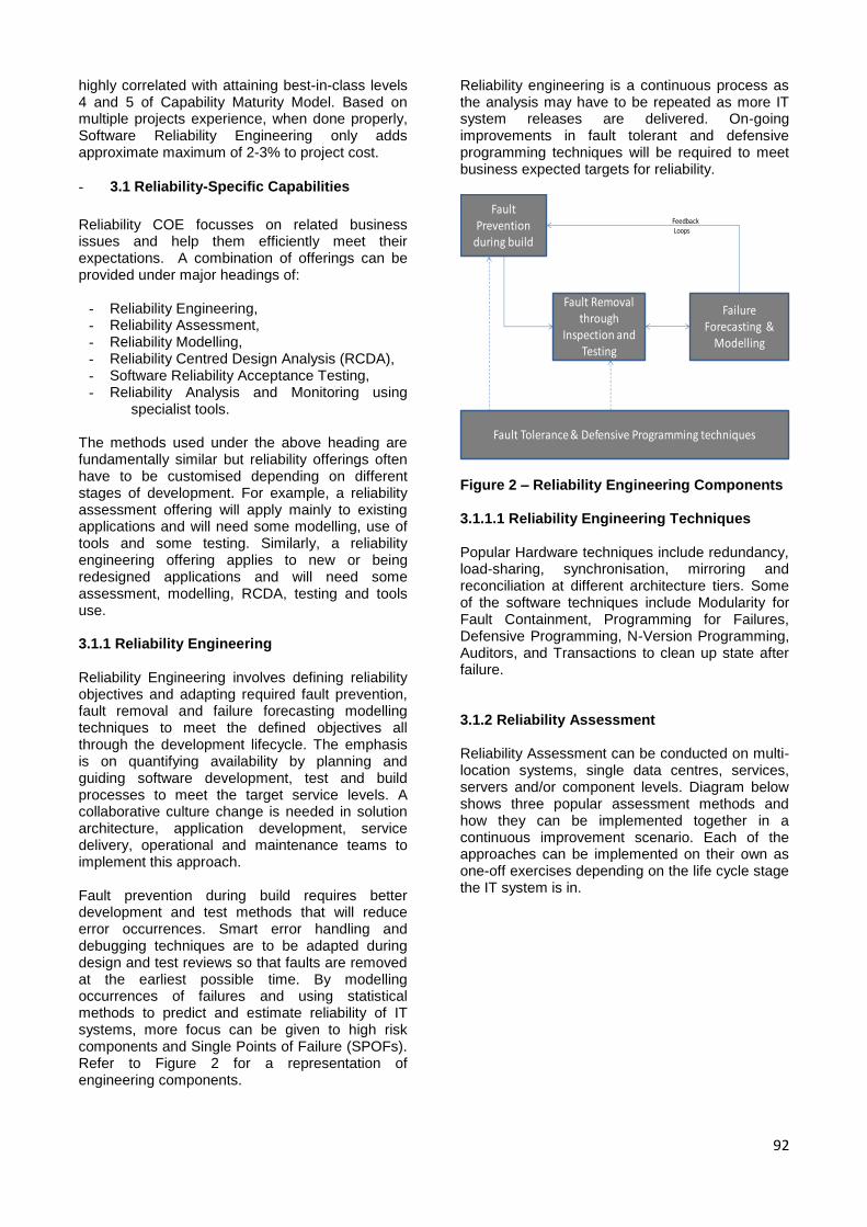
92

highly correlated with attaining best-in-class levels 4 and 5 of Capability Maturity Model. Based on multiple projects experience, when done properly, Software Reliability Engineering only adds approximate maximum of 2-3% to project cost.

- 3.1 Reliability-Specific Capabilities

Reliability COE focusses on related business issues and help them efficiently meet their expectations. A combination of offerings can be provided under major headings of:

- Reliability Engineering, - Reliability Assessment, - Reliability Modelling, - Reliability Centred Design Analysis (RCDA), - Software Reliability Acceptance Testing, - Reliability Analysis and Monitoring using

specialist tools. The methods used under the above heading are fundamentally similar but reliability offerings often have to be customised depending on different stages of development. For example, a reliability assessment offering will apply mainly to existing applications and will need some modelling, use of tools and some testing. Similarly, a reliability engineering offering applies to new or being redesigned applications and will need some assessment, modelling, RCDA, testing and tools use. 3.1.1 Reliability Engineering Reliability Engineering involves defining reliability objectives and adapting required fault prevention, fault removal and failure forecasting modelling techniques to meet the defined objectives all through the development lifecycle. The emphasis is on quantifying availability by planning and guiding software development, test and build processes to meet the target service levels. A collaborative culture change is needed in solution architecture, application development, service delivery, operational and maintenance teams to implement this approach. Fault prevention during build requires better development and test methods that will reduce error occurrences. Smart error handling and debugging techniques are to be adapted during design and test reviews so that faults are removed at the earliest possible time. By modelling occurrences of failures and using statistical methods to predict and estimate reliability of IT systems, more focus can be given to high risk components and Single Points of Failure (SPOFs). Refer to Figure 2 for a representation of engineering components.

Reliability engineering is a continuous process as the analysis may have to be repeated as more IT system releases are delivered. On-going improvements in fault tolerant and defensive programming techniques will be required to meet business expected targets for reliability.

Figure 2 – Reliability Engineering Components 3.1.1.1 Reliability Engineering Techniques Popular Hardware techniques include redundancy, load-sharing, synchronisation, mirroring and reconciliation at different architecture tiers. Some of the software techniques include Modularity for Fault Containment, Programming for Failures, Defensive Programming, N-Version Programming, Auditors, and Transactions to clean up state after failure. 3.1.2 Reliability Assessment Reliability Assessment can be conducted on multi-location systems, single data centres, services, servers and/or component levels. Diagram below shows three popular assessment methods and how they can be implemented together in a continuous improvement scenario. Each of the approaches can be implemented on their own as one-off exercises depending on the life cycle stage the IT system is in.

Fault Prevention

during build

Fault Removal through

Inspection and Testing

Failure Forecasting &

Modelling

Fault Tolerance & Defensive Programming techniques

FeedbackLoops

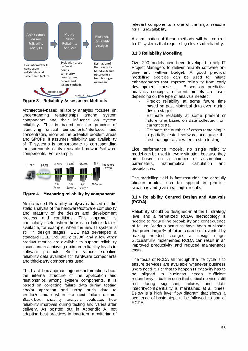
93

Figure 3 – Reliability Assessment Methods Architecture-based reliability analysis focuses on understanding relationships among system components and their influence on system reliability. This is based on the process of identifying critical components/interfaces and concentrating more on the potential problem areas and SPOFs. It assumes reliability and availability of IT systems is proportionate to corresponding measurements of its reusable hardware/software components. For example,

Figure 4 – Measuring reliability by components Metric based Reliability analysis is based on the static analysis of the hardware/software complexity and maturity of the design and development process and conditions. This approach is particularly useful when there is no failure data is available, for example, when the new IT system is still in design stages. IEEE had developed a standard IEEE Std. 982.2 (1988) and a few other product metrics are available to support reliability assessors in achieving optimum reliability levels in software products. Similar vendor supplied reliability data available for hardware components and third-party components used. The black box approach ignores information about the internal structure of the application and relationships among system components. It is based on collecting failure data during testing and/or operation and using such data to predict/estimate when the next failure occurs. Black-box reliability analysis evaluates how reliability improves during testing and varies after delivery. As pointed out in Appendix A, not adapting best practices in long-term monitoring of

relevant components is one of the major reasons for IT unavailability. A combination of these methods will be required for IT systems that require high levels of reliability. 3.1.3 Reliability Modelling Over 200 models have been developed to help IT Project Managers to deliver reliable software on-time and with-in budget. A good practical modelling exercise can be used to initiate enhancements that improve reliability from early development phase. Based on predictive analytics concepts, different models are used depending on the type of analysis needed:

- Predict reliability at some future time based on past historical data even during design stages,

- Estimate reliability at some present or future time based on data collected from current tests,

- Estimate the number of errors remaining in a partially tested software and guide the test manager as to when to stop testing.

Like performance models, no single reliability model can be used in every situation because they are based on a number of assumptions, parameters, mathematical calculation and probabilities. The modelling field is fast maturing and carefully chosen models can be applied in practical situations and give meaningful results. 3.1.4 Reliability Centred Design and Analysis (RCDA) Reliability should be designed-in at the IT strategy level and a formalized RCDA methodology is needed to reduce the probability and consequence of failure. Various statistics have been published that prove large % of failures can be prevented by making needed changes at design stage. Successfully implemented RCDA can result in an improved productivity and reduced maintenance costs. The focus of RCDA all through the life cycle is to ensure services are available whenever business users need it. For that to happen IT capacity has to be aligned to business needs, sufficient redundancy is built-in such that critical services still run during significant failures and data integrity/confidentiality is maintained at all times. Below is a high level flow diagram that shows a sequence of basic steps to be followed as part of RCDA:

Black box Reliability Analysis

Metric-based

Reliability Analysis

Architecture -based

Reliability Analysis

Estimation of the reliability based on failure observations from testing or operation

Evaluation based on function points, complexity, development process and testing methods

Evaluation of the IT component reliabilities and system architecture

Feedback Loop

Feedback Loop

Web Server

App Server 1

DB Server

97.99% 97.7% 98.99% 99.9% 98.99% End-to-end 97.7%

Intranet

App Server 2

98%

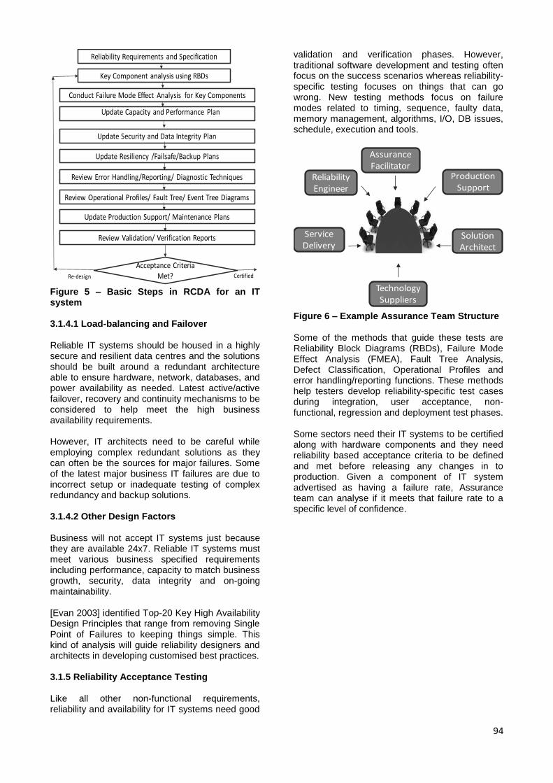
94

Figure 5 – Basic Steps in RCDA for an IT system 3.1.4.1 Load-balancing and Failover Reliable IT systems should be housed in a highly secure and resilient data centres and the solutions should be built around a redundant architecture able to ensure hardware, network, databases, and power availability as needed. Latest active/active failover, recovery and continuity mechanisms to be considered to help meet the high business availability requirements. However, IT architects need to be careful while employing complex redundant solutions as they can often be the sources for major failures. Some of the latest major business IT failures are due to incorrect setup or inadequate testing of complex redundancy and backup solutions. 3.1.4.2 Other Design Factors Business will not accept IT systems just because they are available 24x7. Reliable IT systems must meet various business specified requirements including performance, capacity to match business growth, security, data integrity and on-going maintainability. [Evan 2003] identified Top-20 Key High Availability Design Principles that range from removing Single Point of Failures to keeping things simple. This kind of analysis will guide reliability designers and architects in developing customised best practices. 3.1.5 Reliability Acceptance Testing Like all other non-functional requirements, reliability and availability for IT systems need good

validation and verification phases. However, traditional software development and testing often focus on the success scenarios whereas reliability-specific testing focuses on things that can go wrong. New testing methods focus on failure modes related to timing, sequence, faulty data, memory management, algorithms, I/O, DB issues, schedule, execution and tools.

Figure 6 – Example Assurance Team Structure Some of the methods that guide these tests are Reliability Block Diagrams (RBDs), Failure Mode Effect Analysis (FMEA), Fault Tree Analysis, Defect Classification, Operational Profiles and error handling/reporting functions. These methods help testers develop reliability-specific test cases during integration, user acceptance, non-functional, regression and deployment test phases. Some sectors need their IT systems to be certified along with hardware components and they need reliability based acceptance criteria to be defined and met before releasing any changes in to production. Given a component of IT system advertised as having a failure rate, Assurance team can analyse if it meets that failure rate to a specific level of confidence.

Reliability Requirements and Specification

Key Component analysis using RBDs

Conduct Failure Mode Effect Analysis for Key Components

Update Security and Data Integrity Plan

Update Resiliency /Failsafe/Backup Plans

Review Error Handling/Reporting/ Diagnostic Techniques

Review Operational Profiles/ Fault Tree/ Event Tree Diagrams

Update Production Support/ Maintenance Plans

Review Validation/ Verification Reports

Acceptance Criteria Met? CertifiedRe-design

Update Capacity and Performance Plan

Assurance Facilitator

Reliability Engineer

Service Delivery

Production Support

Solution Architect

Technology Suppliers

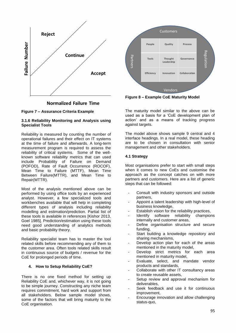
95

Figure 7 – Assurance Criteria Example 3.1.6 Reliability Monitoring and Analysis using Specialist Tools Reliability is measured by counting the number of operational failures and their effect on IT systems at the time of failure and afterwards. A long-term measurement program is required to assess the reliability of critical systems. Some of the well-known software reliability metrics that can used include Probability of Failure on Demand (POFOD), Rate of Fault Occurrence (ROCOF), Mean Time to Failure (MTTF), Mean Time Between Failure(MTTR), and Mean Time to Repair(MTTR). Most of the analysis mentioned above can be performed by using office tools by an experienced analyst. However, a few specialized tools and workbenches available that will help in completing different types of analysis including reliability modelling and estimation/prediction. Partial list of these tools is available in references [Kishor 2013, Goel 1985]. Prediction/estimation using these tools need good understanding of analytics methods and basic probability theory. Reliability specialist team has to master the tool related skills before recommending any of them to the customer area. Often tools related skills result in continuous source of budgets / revenue for the CoE for prolonged periods of time.

4. How to Setup Reliability CoE?

There is no one fixed method for setting up Reliability CoE and, whichever way, it is not going to be simple journey. Constructing any niche team requires commitment, hard work and support from all stakeholders. Below sample model shows, some of the factors that will bring maturity to the CoE organisation.

Figure 8 – Example CoE Maturity Model The maturity model similar to the above can be used as a basis for a ‘CoE development plan of action’ and as a means of tracking progress against targets. The model above shows sample 9 central and 4 interface headings. In a real model, these heading are to be chosen in consultation with senior management and other stakeholders. 4.1 Strategy Most organisations prefer to start with small steps when it comes to new CoEs and customise the approach as the concept catches on with more partners and customers. Here are a list of generic steps that can be followed:

- Consult with industry sponsors and outside partners,

- Appoint a talent leadership with high-level of business knowledge,

- Establish vision for the reliability practices, - Identify software reliability champions

internally and customer areas, - Define organisation structure and secure

funding, - Start building a knowledge repository and

sharing mechanisms, - Develop action plan for each of the areas

mentioned in the maturity model, - Develop strict metrics for each area

mentioned in maturity model, - Evaluate, select, and mandate vendor

products and standards, - Collaborate with other IT consultancy areas

to create reusable assets, - Setup review and approval mechanism for

deliverables, - Seek feedback and use it for continuous

improvement, - Encourage innovation and allow challenging

status-quo,

Accept

Continue

Reject

Normalized Failure Time

Failu

re N

um

be

r People Quality Process

Tools Thought Leadership

Governance

Efficiency Innovation Collaboration

Customers

Vendors

Partners

Regu

lation

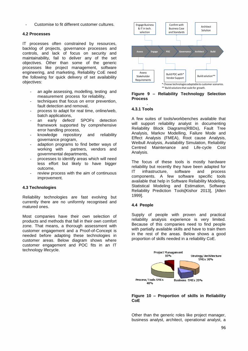
96

- Customise to fit different customer cultures.

4.2 Processes IT processes often constrained by resources, backlog of projects, governance processes and controls, and lack of focus on security and maintainability, fail to deliver any of the set objectives. Other than some of the generic processes like project management, software engineering, and marketing, Reliability CoE need the following for quick delivery of set availability objectives:

- an agile assessing, modelling, testing and measurement process for reliability,

- techniques that focus on error prevention, fault detection and removal,

- process to adapt for real time, online/web, batch applications,

- an early defect/ SPOFs detection framework supported by comprehensive error handling process,

- knowledge repository and reliability governance program,

- adaption programs to find better ways of working with partners, vendors and governmental departments,

- processes to identify areas which will need less effort but likely to have bigger outcome,

- review process with the aim of continuous improvement.

4.3 Technologies Reliability technologies are fast evolving but currently there are no uniformly recognised and matured ones. Most companies have their own selection of products and methods that fall in their own comfort zone. That means, a thorough assessment with customer engagement and a Proof-of-Concept is needed before adapting these technologies in customer areas. Below diagram shows where customer engagement and POC fits in an IT technology lifecycle.

Figure 9 – Reliability Technology Selection Process

- 4.3.1 Tools A few suites of tools/workbenches available that will support reliability analyst in documenting Reliability Block Diagrams(RBDs), Fault Tree Analysis, Markov Modelling, Failure Mode and Effect Analysis (FMEA), Root cause Analysis, Weibull Analysis, Availability Simulation, Reliability Centred Maintenance and Life-cycle Cost Analysis. The focus of these tools is mostly hardware reliability but recently they have been adapted for IT infrastructure, software and process components. A few software specific tools available that help in Software Reliability Modeling, Statistical Modeling and Estimation, Software Reliability Prediction Tools[Kishor 2013], [Allen 1999]. 4.4 People Supply of people with proven and practical reliability analysis experience is very limited. Because of this companies need to find people with partially available skills and have to train them in the rest of the areas. Below shows a good proportion of skills needed in a reliability CoE.

Figure 10 – Proportion of skills in Reliability CoE Other than the generic roles like project manager, business analyst, architect, operational analyst, a

Assess Engage POC Governance Architect Build

Assess Stakeholder

Requirements

Engage Business & IT in tech.

selection

Build POC with* Vendor Support

Confirm with Business Case and Standards

Architect Solution

Build solution**

* Choose technologies adaptable to customer scenarios. ** Build solutions that scale for growth.

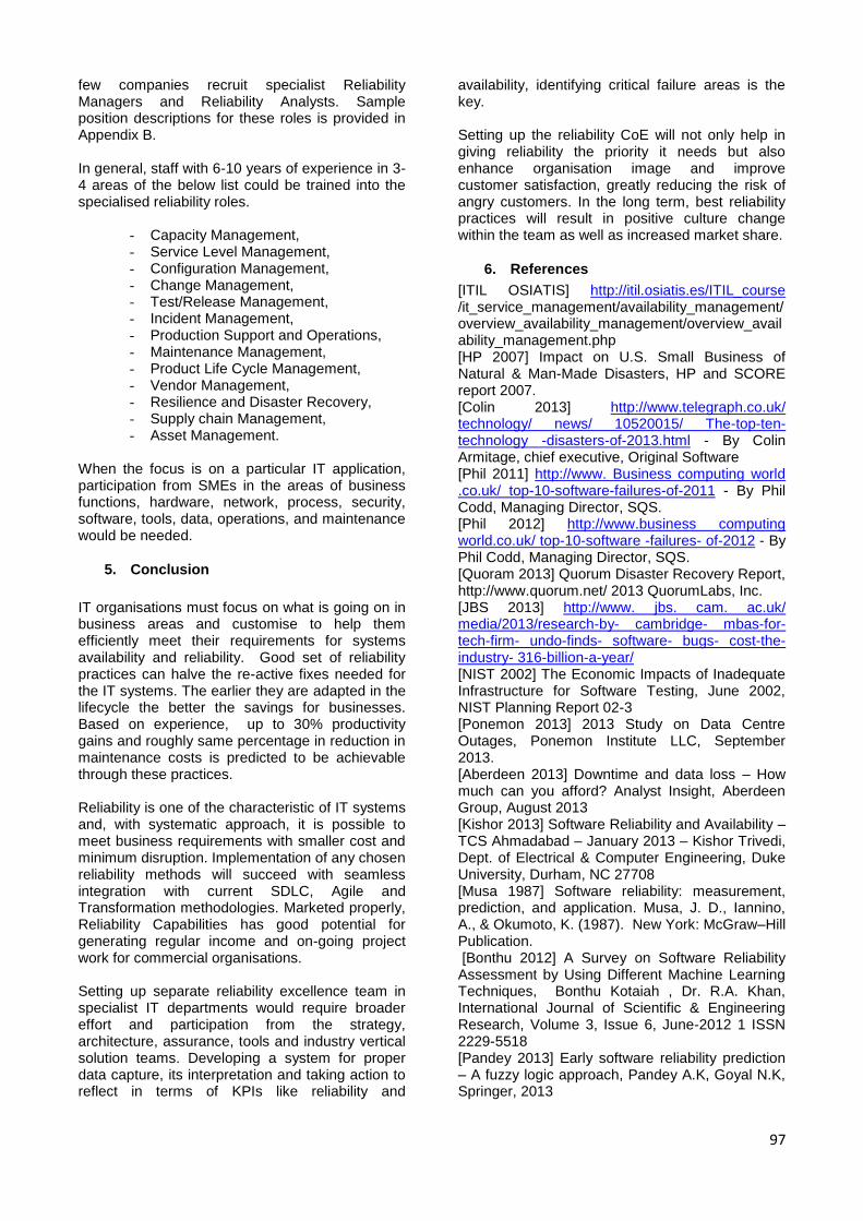
97

few companies recruit specialist Reliability Managers and Reliability Analysts. Sample position descriptions for these roles is provided in Appendix B. In general, staff with 6-10 years of experience in 3-4 areas of the below list could be trained into the specialised reliability roles.

- Capacity Management, - Service Level Management, - Configuration Management, - Change Management, - Test/Release Management, - Incident Management, - Production Support and Operations, - Maintenance Management, - Product Life Cycle Management, - Vendor Management, - Resilience and Disaster Recovery, - Supply chain Management, - Asset Management.

When the focus is on a particular IT application, participation from SMEs in the areas of business functions, hardware, network, process, security, software, tools, data, operations, and maintenance would be needed.

5. Conclusion

IT organisations must focus on what is going on in business areas and customise to help them efficiently meet their requirements for systems availability and reliability. Good set of reliability practices can halve the re-active fixes needed for the IT systems. The earlier they are adapted in the lifecycle the better the savings for businesses. Based on experience, up to 30% productivity gains and roughly same percentage in reduction in maintenance costs is predicted to be achievable through these practices. Reliability is one of the characteristic of IT systems and, with systematic approach, it is possible to meet business requirements with smaller cost and minimum disruption. Implementation of any chosen reliability methods will succeed with seamless integration with current SDLC, Agile and Transformation methodologies. Marketed properly, Reliability Capabilities has good potential for generating regular income and on-going project work for commercial organisations. Setting up separate reliability excellence team in specialist IT departments would require broader effort and participation from the strategy, architecture, assurance, tools and industry vertical solution teams. Developing a system for proper data capture, its interpretation and taking action to reflect in terms of KPIs like reliability and

availability, identifying critical failure areas is the key. Setting up the reliability CoE will not only help in giving reliability the priority it needs but also enhance organisation image and improve customer satisfaction, greatly reducing the risk of angry customers. In the long term, best reliability practices will result in positive culture change within the team as well as increased market share.

6. References

[ITIL OSIATIS] http://itil.osiatis.es/ITIL_course /it_service_management/availability_management/overview_availability_management/overview_availability_management.php [HP 2007] Impact on U.S. Small Business of Natural & Man-Made Disasters, HP and SCORE report 2007. [Colin 2013] http://www.telegraph.co.uk/ technology/ news/ 10520015/ The-top-ten-technology -disasters-of-2013.html - By Colin Armitage, chief executive, Original Software [Phil 2011] http://www. Business computing world .co.uk/ top-10-software-failures-of-2011 - By Phil Codd, Managing Director, SQS. [Phil 2012] http://www.business computing world.co.uk/ top-10-software -failures- of-2012 - By Phil Codd, Managing Director, SQS. [Quoram 2013] Quorum Disaster Recovery Report, http://www.quorum.net/ 2013 QuorumLabs, Inc. [JBS 2013] http://www. jbs. cam. ac.uk/ media/2013/research-by- cambridge- mbas-for-tech-firm- undo-finds- software- bugs- cost-the-industry- 316-billion-a-year/ [NIST 2002] The Economic Impacts of Inadequate Infrastructure for Software Testing, June 2002, NIST Planning Report 02-3 [Ponemon 2013] 2013 Study on Data Centre Outages, Ponemon Institute LLC, September 2013. [Aberdeen 2013] Downtime and data loss – How much can you afford? Analyst Insight, Aberdeen Group, August 2013 [Kishor 2013] Software Reliability and Availability – TCS Ahmadabad – January 2013 – Kishor Trivedi, Dept. of Electrical & Computer Engineering, Duke University, Durham, NC 27708 [Musa 1987] Software reliability: measurement, prediction, and application. Musa, J. D., Iannino, A., & Okumoto, K. (1987). New York: McGraw–Hill Publication. [Bonthu 2012] A Survey on Software Reliability Assessment by Using Different Machine Learning Techniques, Bonthu Kotaiah , Dr. R.A. Khan, International Journal of Scientific & Engineering Research, Volume 3, Issue 6, June-2012 1 ISSN 2229-5518 [Pandey 2013] Early software reliability prediction – A fuzzy logic approach, Pandey A.K, Goyal N.K, Springer, 2013

98

[Pham 2006] System software reliability, reliability engineering series. Pham, H. (2006). London: Springer. [Lyu 1996] Handbook of software reliability engineering. Lyu, M. R. (1996). NY: McGraw–Hill/IEE Computer Society Press. [Goel 1985] Software reliability models: assumptions, limitations, and applicability. Goel, A. L. (1985). IEEE Transaction on Software Engineering, SE–11(12), 1411–1423. [Allen 1999] Software Reliability and Risk Management: Techniques and Tools. Allen Nikora and Michael Lyu, tutorial presented at the 1999 International Symposium on Software Reliability Engineering.

[Ulrik 2010] Availability of enterprise IT systems –

an expert-based Bayesian model, Ulrik Franke,

Pontus Johnson, Johan König, Liv Marcks von Würtemberg: Proc. Fourth International Workshop on Software Quality and Maintainability (WSQM 2010), Madrid [Evan 2003] Blueprint for High Availability – Evan Marcus/Hal Stern – 2003 – Wiley Publications

7. Acknowledgement

Authors are grateful to Girish Chaudhari, Peter Andrew, Carl Borthwick and Jonathan Wright who reviewed the material when it was first prepared for an internal team discussion. We would also like to thank Prajakta Vijay Bhatt and the anonymous CMG referees for their comments which have helped make this paper better.

99

Appendix A: Surveyed Reasons for Unavailability

A survey among a few academic availability experts in 2010 ranked reasons for unavailability of enterprise IT

systems [Ulrik 2010]. They identified the lack of best practices in the following areas are the causes:

• Monitoring of the relevant components • Requirements and procurement • Operations • Avoidance of network failures, internal application failures, and external services that fail • Network redundancy • Technical solution of backup, and process solution of backup • Physical location, • Infrastructure redundancy • Storage architecture redundancy • Change Control

[Evan 2003] identified investment in the following areas will help improve the availability of IT systems.

• Good systems and admin procedures • Reliable backups • Disk and volume management • Networking • Local Environment • Client Management • Services and application • Failovers • Replication

Even though these studies does not apply in all cases, they provide useful guidelines for architects and designers of IT systems. This paper proposes more structured approach for availability management that applies to most business organisations.

100

Appendix B – Sample Reliability Engineer Position Descriptions

Senior Reliability Engineer – Technical IT Infrastructure

This position is located within xxx Team in Reliability, Maintainability and Testability Support

Discipline,

xxx team has a role of increasing the availability and reducing the through life cost of ownership of IT

systems for customers.

Main responsibilities:

Own end-to-end availability and performance of customer critical services from infrastructure point of

view,

Ensure five 9s reliable experience for IT systems users located in UK and abroad,

Liaison with customer teams and other partners to obtain Reliability data,

Analyse, Model and interpret arising data to forecast the reliability of customer IT systems,

Utilisation of reliability data to produce analysis and system performance reports for customers,

Capable of technical deep-dives into code, networking, operating systems and storage problem areas,

Respond to and resolve emergent service problems to prevent problem recurrence,

Liaising with Design, Support, Maintenance, Procurement and Commercial functions to identify

suitable recommendations for improvements,

Understanding and interpreting IT maintenance and support information to identify root causes of IT

failure,

Attendance at customer high-level service reviews and support root cause analysis,

Detailed IT systems analysis to support releases in different production environments,

Representing xxx team in internal and external customer meetings,

Participate in service capacity planning, demand forecasting, software performance analysis and

system tuning activities

Minimum qualifications

BS degree in Computer Science or related field or equivalent practical experience,

Proven experience in similar role in a commercial organisation, using formal reliability tools and

procedures,

Good understanding of reliability, maintainability and testability practices

Preferred qualifications

MS degree in Computer Science or related field,

Experience with different M/F, servers, desktop systems administration and logistics,

Expertise in data structures, algorithms and basic statistical probability theory,

Expertise in analysing and troubleshooting large-scale distributed systems,

Knowledge of network analysis, performance and application issues using standard tools: BMC

Patrol, Teamquest or similar,

Experience in a high-volume or critical production service environment,

Sound understanding of understanding of IT life-cycle management and maturity gates,

Strong leadership, communication, report writing, and presentation skills.

101

Senior Reliability Engineer – Software Engineering

This position is located within the xxx Team in Reliability, Maintainability and Testability Support

Discipline,

xxx team has a role of increasing the availability and reducing the through life cost of ownership of IT

systems for customers.

Main responsibilities:

Own end-to-end availability and performance of customer critical services from software design point

of view,

Manage availability, latency, scalability and efficiency of customer services by engineering reliability

into software and systems,

Review and influence ongoing design, architecture, standards and methods for operating services and

systems,

Work in conjunction with software engineers, systems administrators, network engineers and

hardware teams to derive detailed reliability requirements,

Identify metrics and drive initiatives to improve the quality of design processes,

Understanding of fault prevention, fault removal, fault tolerance & defensive programming design

techniques,

Liaison with customer teams and other partners to build five 9s reliability into software delivery

procedures,

Capable of technical deep-dives into code, networking, operating systems and storage design

problem areas,

Attendance at customer high-level IT design reviews,

Representing xxx team in internal and external customer meetings,

Participate in capacity planning, demand forecasting, software performance analysis and system

tuning activities.

Minimum qualifications

BS degree in Computer Science or related field or equivalent practical experience,

Proven experience in similar role in a commercial organisation, using formal reliability tools and

procedures,

Good understanding of reliability, maintainability and testability practices.

Preferred qualifications

MS degree in Computer Science or related field,

Expertise in complexity analysis and basic statistical probability theory,

Expertise in designing end-to-end large-scale distributed systems with full resilience,

Experience in end-to-end infrastructure, data, applications, security and service design,

Experience in a high-volume or critical production service environment,

Sound understanding of understanding of IT life-cycle management and maturity gates,

Strong leadership, communication, report writing, and presentation skills