University of Ioannina

School of Natural Sciences

Physics Department

PhD Thesis

Elastic scattering and reaction

mechanisms for the system 7Be+28Si at

near barrier energies

Author:

Onoufrios Sgouros

Supervisor:

Prof. Athina Pakou

May 2017

Advisory committee:

1. Athina Pakou (Supervisor)

Emeritus Professor

Physics Department

University of Ioannina

2. Nicolas Alamanos

Professor

Deputy Director of IRFU

Research Director at CEA-SACLAY

France

3. Efstathios Stiliaris

Associate Professor

Physics Department

University of Athens

Review committee:

1. Athina Pakou: Emeritus Professor - Physics Department - University of Ioannina

2. Nicolas Alamanos: Professor - Deputy Director of IRFU - Research Director at CEA-

SACLAY, France

3. Efstathios Stiliaris: Associate Professor - Physics Department - University of Athens

4. Dimitra Pierroutsakou: Senior Researcher - INFN Napoli, Italy

5. Nicholas Keeley: Associate Professor - NCBJ, Poland

6. Nikolaos Nicolis: Associate Professor - Physics Department - University of Ioannina

7. Nikolaos Patronis: Assistant Professor - Physics Department - University of Ioannina

To my parents

Giorgo and Maria

Contents

Acknowledgements . . . . . . . . . . . . . . . . . . . . . . . . . . . . . . . . . . . . 1

Abstract . . . . . . . . . . . . . . . . . . . . . . . . . . . . . . . . . . . . . . . . . . 3

Introduction . . . . . . . . . . . . . . . . . . . . . . . . . . . . . . . . . . . . . . . . 7

1 Theory 13

1.1 Elastic Scattering . . . . . . . . . . . . . . . . . . . . . . . . . . . . . . . . . . 13

1.1.1 Scattering by a short range central potential . . . . . . . . . . . . . . . 14

1.1.2 Continuum Discretized Coupled Channels Calculations . . . . . . . . . 17

1.1.3 Optical Model . . . . . . . . . . . . . . . . . . . . . . . . . . . . . . . . 21

1.1.4 Threshold Anomaly and Dispersion Relations . . . . . . . . . . . . . . 25

1.2 Reaction Mechanisms . . . . . . . . . . . . . . . . . . . . . . . . . . . . . . . . 26

1.2.1 Direct Reactions . . . . . . . . . . . . . . . . . . . . . . . . . . . . . . 27

1.2.2 Compound Nucleus Reactions . . . . . . . . . . . . . . . . . . . . . . . 34

2 Experimental Details 39

2.1 The EXOTIC facility . . . . . . . . . . . . . . . . . . . . . . . . . . . . . . . . 39

2.1.1 The dipole . . . . . . . . . . . . . . . . . . . . . . . . . . . . . . . . . . 40

2.1.2 The Wien filter . . . . . . . . . . . . . . . . . . . . . . . . . . . . . . . 41

2.2 Detection systems and electronics . . . . . . . . . . . . . . . . . . . . . . . . . 42

2.2.1 Silicon detectors . . . . . . . . . . . . . . . . . . . . . . . . . . . . . . . 43

2.2.2 Parallel Plate Avalanche Counters . . . . . . . . . . . . . . . . . . . . . 43

2.2.3 Double Sided Silicon Strip Detectors (DSSSD) and the EXPADES array 47

2.2.4 The trigger of the experiment . . . . . . . . . . . . . . . . . . . . . . . 50

2.3 Experimental setup and procedure . . . . . . . . . . . . . . . . . . . . . . . . 50

3 Data Reduction 55

3.1 Energy calibration . . . . . . . . . . . . . . . . . . . . . . . . . . . . . . . . . 55

3.2 Determination of the elastic scattering cross sections . . . . . . . . . . . . . . 57

3.3 Determination of the reaction cross sections . . . . . . . . . . . . . . . . . . . 61

3.3.1 α - particle production cross sections . . . . . . . . . . . . . . . . . . . 62

3.3.2 3He production cross sections . . . . . . . . . . . . . . . . . . . . . . . 64

4 Theoretical Analysis 71

4.1 Elastic Scattering . . . . . . . . . . . . . . . . . . . . . . . . . . . . . . . . . . 71

4.1.1 Optical Model Analysis . . . . . . . . . . . . . . . . . . . . . . . . . . . 71

4.1.2 Energy evolution of the optical potential parameters . . . . . . . . . . 75

4.1.3 Total reaction cross sections . . . . . . . . . . . . . . . . . . . . . . . . 76

4.1.4 Continuum Discretized Coupled Channels Calculations . . . . . . . . . 80

4.2 Reaction Mechanisms . . . . . . . . . . . . . . . . . . . . . . . . . . . . . . . . 85

4.2.1 Fusion Cross Sections . . . . . . . . . . . . . . . . . . . . . . . . . . . . 85

4.2.2 Direct Reactions Cross Sections . . . . . . . . . . . . . . . . . . . . . . 91

4.2.3 DWBA Calculations . . . . . . . . . . . . . . . . . . . . . . . . . . . . 93

5 Conclusions - Summary 99

References 103

A Event by event analysis code 113

B Simulation Code 117

C Tabulated cross sections 121

D Error calculation formulas 127

E ΔE-E technique 131

Acknowledgements

I would like to thank all of those who have supported and assisted me during my PhD

studies.

First of all, I would like to express my sincere gratitude to Professor of Nuclear Physics

Athina Pakou, my supervisor, for her precious guidance and help throughout my studies, for

proposing the subject of my PhD thesis and for supporting my efforts during my studies. I

feel honored for being a student of Professor A. Pakou all these years, starting with my under-

graduate diploma thesis until my PhD studies, where she generously shared her knowledge by

introducing me to the appropriate experimental and theoretical techniques, necessary in the

Nuclear Physics field, while she still keeps motivating me to bring the best out of myself.

Also, I would like to express my sincere thanks to the members of the advisory commit-

tee, Professor Nicolas Alamanos and Associate Professor Efstathios Stiliaris for the generous

assistance they provided.

I would like also to thank the EXOTIC group for their substantial contribution during

the experiment and in particular Prof. Cosimo Signorini and the head of the EXOTIC group

Dr. Dimitra Pierroutsakou for hosting this experiment and for making available the EXOTIC

facility, Dr. Marco Mazzocco who was responsible for the production of the secondary 7Be

radioactive beam and Dr. Alfonso Boiano and Dr. Ciro Boiano for setting up the electronic

chain of the experiment and for their continuous assistance with the emerging problems in

the electronics during the experiment. Also, I would like to thank Assoc. Prof. Marco La

Commara, Dr. Tina Parascandolo, Dr. Emanuele Strano, Dr. Domenico Torresi and all the

rest of the participants for their unreserved assistance during the experiment.

I would like to extend my sincere and warm thanks to Professor Krzysztof Rusek and As-

sociate Professor Nicholas Keeley for the theoretical support and in particular, for introducing

me to the CDCC calculations with the code FRESCO during an one week seminar in Warsaw.

Working with them has been a very profitable experience. Also, I would like to thank Professor

Krzysztof Rusek for his generous hospitality in the dormitories of the Heavy Ion Laboratory

during my staying in Warsaw. I could not omit the Associate Professor Nikolaos Nicolis from

the Nuclear Physics Laboratory of the University of Ioannina, who provided the theoretical

support regarding the compound nucleus calculations, performed via code PACE2.

Also, I would like to thank Associate Professor Efstathios Stiliaris and his group for intro-

ducing me to Geant simulations using the program GATE .

1

Moreover, I am grateful to Dr. Angel Miguel Sanchez-Benıtez and Dr. Gloria Marquınez-

Duran for their help regarding the pixel analysis.

I would like to extend my sincere thanks to Prof. Francesco Cappuzzello who provided

me the opportunity to get familiar with the analysis of experimental data acquired with the

MAGNEX spectrometer in conjunction with the neutron detector array EDEN, during a three-

month ERASMUS traineeship in Catania (LNS). Collaborating with him and his group helped

me to broaden further my skills from various perspectives.

Furthermore, I would like to thank my fellow team members Dr. Konstantina Zerva and

Ms. Chrysoula Betsou for their collaborative and friendly spirit but especially my friend and

fellow worker Dr. Vasileio Soukera for the thoughtful discussions not only in the field of Physics

and for being a nice company at the office all these years.

In addition, I would like to thank the members of the review committee for reading carefully

this manuscript and for the insightful comments/corrections they made.

Last but not least, I would like to thank my family, my parents Giorgo and Maria and my

brother Gianni but especially my parents, for supporting my efforts all these years and never

stopped to have faith on me.

2

Abstract

The present work refers to the study of elastic scattering and reaction products for the

system 7Be + 28Si at near barrier energies, namely 13.2, 17.2, 19.8 and 22.0 MeV(E/VC.b.=

1.14, 1.48, 1.71, 1.90). The goal of this work is to probe the energy dependence of the op-

tical potential as well as the interplay between direct and compound nucleus mechanisms.

The experiment was visualized at the EXOTIC beam line of the Istituto Nazionale di Fisica

Nucleare - Laboratori Nazionali di Legnaro (INFN-LNL) in Italy. The 7Be secondary beam

was produced via the in-flight technique through the 1H(7Li,7Be)n reaction, where a 7Li pri-

mary beam with an intensity of (100-150)pnA, delivered by the LNL XTU-TANDEM Van

de Graaff accelerator, impinged on a primary hydrogen gas target. The produced 7Be beam

was separated from other contaminants by means of a bending dipole and a Wien filter and

it was directed into the scattering chamber, impinging on a 28Si target. A 208Pb target was

also used for normalization purposes. The various ejectiles were collected by six ∆E-E tele-

scopes of the detector array of the EXOTIC facility, EXPADES(EXotic PArticle DEtection

System), placed at symmetrical position to balance any beam divergence and to improve the

statistics of the measurement. The ∆E stage of the telescopes was a Double Sided Silicon

Strip Detector (DSSSD) (45-60)µm thick, while the E stage was a DSSSD ∼ 300 µm thick.

Also, our experimental setup included two X-Y position sensitive Parallel Plate Avalanche

Counters (PPAC’s) for monitoring the secondary beam profile and providing information for

an event by event reconstruction of the beam particle and elastic scattering trajectories.

The analysis of the elastic scattering data was performed by means of an event by event

analysis code using the two PPAC signals to enable reconstruction of the beam ray and elastic

scattering trajectories. The position of the reaction vertex on the target and of the DSSSD

X-Y strip struck by the elastically scattered nucleus were thus unambiguously defined for each

event, leading to a more precise assignment of angle (see Appendix A). Events with the same

angle or with an angle inside an angular range corresponding to the dimensions of a particular

strip of each EXPADES detector (∆θ ∼2o) were summed up and were appropriately normalized

for the deduction of differential cross sections.

The elastic scattering data were analyzed into the optical model framework following the

same method as adopted previously for 6,7Li + 28Si using the code ECIS. The real part of

the optical potential was derived in a double folding model using the microscopic BDM3Y1

interaction. Although the microscopic BDM3Y1 interaction is purely real, assuming that the

imaginary part of the optical potential presents the same radial shape as the real one, the

3

same folded potential was adopted but with a different normalization factor. The normaliza-

tion factors for the real and the imaginary part were fitted to the data and the energy evolution

of these parameters was deduced. Due to the large errors, it was not possible to draw firm

conclusions solely from the elastic scattering data but only in conjunction with the α - par-

ticle production ones. In principle the trend of the imaginary part obtained from the elastic

scattering data, seems to be compatible with a standard threshold anomaly, with a decreasing

magnitude as we approach the barrier from higher to lower energies. The agreement of the

present data with a dispersion relation cannot be confirmed, as in the critical position of the

real potential, where a peak should appear, we possess only one datum. On the other hand,

taking into account all information relevant to previous data of 6,7Li + 28Si, analyzed in the

same framework as is the present case, we can in principle conclude that both mirror nuclei,7Li and 7Be present the same energy dependence of the optical potential. This is close to the

standard threshold anomaly, from the point of view of the decreasing imaginary potential but

where possibly the dispersion relation does not hold and the real part is consistent with a flat

line independent of energy. This evidence, if combined with the results of the α - production

data, collected at the same experiment, indicates with some confidence the similarity between

the two mirror nuclei.

Our optical model analysis yielded also total reaction cross sections which were found in

very good agreement with the total reaction cross sections deduced from the 3,4He-particle

production, global phenomenological predictions and our CDCC calculations. The last were

performed with the code FRESCO and it was found that the effect of coupling to the ground

state reorientation and excitation of the first excited state of 7Be is weak. Despite a very

small breakup cross section the coupling to continuum was found to be significant but not very

strong. As far as the total reaction cross sections, the compatibility with the phenomenological

predictions and the CDCC calculations indicates the validity of our measurements. It also

supports our results for the energy dependence of the optical potential, since total reaction

cross sections are traditionally used to restrict the imaginary part of the optical potential.

Regarding the reaction mechanisms, the analysis of the data refers to the 3He and 4He

particle production either through a direct or a compound nucleus process. These light reaction

products were able to pass through the ∆E stage of the telescopes and thus, they were well-

discriminated via the ∆E-E technique. The 3He and 4He yields were obtained by applying the

appropriate energy windows on the two dimensional ∆E-E plots. However, due to the thickness

of the ∆E stage of the telescopes, an energy threshold in the detection of the two ions was

introduced. The missing counts were retrieved by comparing the experimental energy spectra

4

with the simulated ones. The simulated energy spectra for the direct processes were generated

by a Monte Carlo code (see Appendix B), while the compound nucleus spectra were produced

via the code PACE2(Projection Angular-momentum Coupled Evaporation

). Then, direct

and the compound nucleus spectra were summed using various assumptions for the ratio direct

to compound nucleus contributions until the best fit to the experimental data was obtained.

After correcting for the missing counts, the differential cross sections for 3He and 4He particle

production were deduced.

The compound nucleus contribution to the 4He-particle production was estimated by re-

normalizing the theoretical angular distributions from evaporated α-particles, calculated via

the statistical model code PACE2, to the data of the backward angle detectors. Subsequently,

using the α-particle multiplicities, obtained with the same statistical model code, fusion cross

sections were deduced. The α-particle multiplicities are sensitive on the choice of the optical

model parameters for the evaporation of α-particles and this may introduce further uncertain-

ties in the fusion cross sections. In this direction, the error in the calculated multiplicities

was estimated adopting three different sets of optical model parameters for the evaporation

of α-particles. The deduced fusion cross sections (appropriately reduced to fusion functions)

were considered in a systematic framework with other stable, weakly bound and radioactive

projectiles on the same or similar mass targets and were found in good agreement between

each other as well as the Universal Fusion Function (UFF) to within an uncertainty band

of 10% to 20%. Moreover, ratios of fusion functions for 6Li to those for 7Li and 7Be were

formed, indicating a hindrance of fusion for 7Li and 7Be with respect to those of 6Li below

the barrier rather than an enhancement. This hindrance was also observed before for 7Li on

various targets and together with the results obtained from our optical model analysis present

a strong evidence for the similarity of 7Be with its mirror nucleus 7Li and not the 6Li one.

The angular distributions for the direct component of the α-production were obtained after

subtracting from the total α experimental angular distributions, the re-normalized theoretical

compound nucleus ones. Comparisons between experimental data and the theoretical angular

distributions for the single neutron pickup, single neutron stripping and breakup showed that

these processes are unable to descibe the bulk of the observed α-particle cross sections. There-

fore, the remaining part was attributed to the 3He stripping reaction although this was not

confirmed via DWBA calculations, due to the lack of the appropriate spectroscopic factors.

Regarding the 3He production, the only two contributing mechanisms are the 4He stripping

and the breakup. Due to the low statistics and the geometrical efficiency of our detector setup,

coincidence events between 3He and 4He particles, a clear signature of an exclusive breakup

5

event, were not recorded. Therefore, integrating the 3He angular distributions, we can pro-

vide an inclusive cross section for both reaction channels although the breakup is predicted

in CDCC calculations to be very small and therefore this cross section is described mainly

by the 4He stripping process. DWBA theoretical calculations are in reasonable qualitative

agreement with the experimental data but underestimate them in absolute magnitudes. The

last was attributted to the fact that absolute spectroscopic factors for α transfer reactions are

ambiguously determined, with factors of 5 or more between values for the same target obtained

with different reactions and at different bombarding energies being common.

Finally, total reaction cross sections were formed as the sum of the direct and fusion cross

sections and the ratio of direct to total reaction cross sections as a function of energy was

deduced. These ratio’s were compared with previous ones for 6,7Li on 28Si, where an increasing

trend approaching the barrier from higher to lower energies is seen. For 7Li larger ratio’s than

in 6Li are observed and our data for 7Be are in quantitative agreement with the data of 7Li

and not 6Li, pointing out to a similarity between the two mirror nuclei. This enhancement of

direct channels versus compound for 7Li and 7Be acts at the expense of fusion resulting in the

fusion hidrance mentioned above.

6

Introduction

This work is part of the curriculum of the Postgraduate Program of the Department of

Physics, University of Ioannina. The research area belongs to the basic direction of Nuclear

Physics and in particular on the subject of elastic scattering and reaction mechanisms at near

barrier energies involving weakly bound nuclei.

Elastic scattering is the simplest process in the nucleus-nucleus collisions. But even in such

“simple” case, the nuclear interactions are far too complicated since the interacting nuclei are

composite systems of many nucleons. A solution to the complex many-body problem of the

interaction of two nuclei may be given by the Optical Model (OM), which approximates the

interaction of two nuclei by the interaction of two structureless particles through an effective

potential. In the Optical Model framework the interaction between two nuclei is represented

by a complex potential, where the real part accounts for the refraction of the incident particles

by the target, while the imaginary part for the absorption of flux out of the elastic channel via

the different reaction mechanisms. Both terms of the optical potential are energy dependent

and in this direction, many studies over the past decades have been devoted to study the

energy dependence of the optical potential through elastic scattering measurements.

At energies well above Coulomb barrier, the energy evolution of the optical potential is

almost energy independent. However, this independence no longer holds while approaching

the vicinity of Coulomb barrier. A first indication for an unusual behavior of the potential in

the vicinity of Coulomb barrier was provided by optical model analyses of elastic scattering for16O + 208Pb [1] and 32S + 40Ca [2]. Subsequently, the term “Threshold Anomaly” (TA) [3–5]

was applied to such cases, where a rapid and localized variation with energy E of the heavy-

ion optical potential appears at barrier. This variation is visualized as a localized peak in

the strength of the real potential, associated with a sharp decrease in the strength of the

imaginary potential as it becomes more and more unimportant to remove flux from the reaction

in this low energy region. The advent of Radioactive Ion Beam (RIB) facilities moved the

interest to predecessor cases with weakly bound but stable projectiles, since direct processes

like breakup and transfer are enhanced for such systems [6–11]. It was believed [4,12,13] that

the polarization potential which is produced by the breakup, as it is repulsive in nature, will

compensate the attractive term, ∆V, of the real potential(V= V0 + ∆V

)which is connected

through a dispersion relation [4, 5] with the imaginary part and which is responsible for the

threshold anomaly. Otherwise, as it is suggested by Satchler [4], the dispersion relation may

be of no use for weakly bound systems, since according to theoretical calculations [12,13], the

7

repulsive contribution of the real part of the potential, is almost independent of beam energy,

while the associated imaginary potential is very small. Indeed, the pioneering experimental

work of elastic scattering with the weakly bound but stable projectiles 6Li and 7Li on 208Pb

and 138Ba targets [14, 15] traced an unusual behavior for 6Li but not with 7Li. It should be

taken into account that the breakup threshold for the first nucleus is only 1.47 MeV, while for

the second is 2.47 MeV. Later on the new manifestation of the anomaly for 6Li, is observed

for 6Li + 28Si [16] and is interpreted in terms of dispersion relations in Ref. [17]. With the

aid of a re-analysis of previous data, it was pointed out in these articles [16,17] the increasing

trend of the imaginary potential approaching the barrier from higher to lower energies for 6Li,

but not for 7Li. This increasing behavior is related via dispersion relations with an almost

flat evolution of the real part of the potential (with a shallow valley at barrier), developing

the bell shape peak at very low energies well below barrier [17–20]. The new manifestation of

the anomaly for 6Li is discussed later in Ref. [21] and named as Breakup Threshold Anomaly

(BTA). By today the new anomaly for 6Li but not for 7Li is well established although not

fully understood and verified in numerous articles for various targets as 27Al [22], 28Si [16,17],58Ni [23], 59Co [24], 64Zn [25], 80Se [26], 90Zr [27], 112,116Sn [28], 138Ba [15], 144Sm [29], 208Pb [14],209Bi [30] and 232Th [31]. A review of these measurements can be found in Ref. [32].

The situation is less clear for radioactive projectiles. Existing measurements are reviewed

in Ref. [8] and concern mainly the neutron rich nucleus 6He and the proton rich nuclei 8B and7Be. Comprehensive work on the energy dependence of the potential via angular distributions

measurements is achieved for 6He on both 208Pb [33,34] and 209Bi [35] targets. The conclusion

is that the potential behavior of 6He is the same as for 6Li, and it can be attributed to the

very low binding energy of the two neutrons to an alpha core of 0.973 MeV. Elastic scattering

measurements with the cocktail radioactive beam(8B, 7Be, 6Li

)on 58Ni were performed in

Notre Dame and the results of the analysis are reported in Ref. [36]. The first conclusion,

although it is given with caution due to the large uncertainties assigned to the potential

parameters, is that both proton rich nuclei, 8B and 7Be present the same trend as 6Li which

was measured and analyzed simultaneously with the radioactive ones. This conclusion is later

re-confirmed for 8B in Ref. [37]. However, the re-analysis of 7Be data [38], including elastic

scattering combined with fusion data, showed that 7Be resembles rather its mirror nucleus

than 6Li, presenting both the usual threshold anomaly. The last measurement appearing

in the literature concerning radioactive projectiles is related again with the proton rich 7Be

nucleus, but on elastic scattering from 27Al [39]. The data were collected in two RIB facilities

of the Universities of Sao Paulo and Notre Dame. Due to the low beam flux the researchers

of [39] had to use very thick targets. Their optical model results suggest an energy independent

8

optical potential around barrier, but this conclusion is given as susceptible to the use of very

thick targets.

In principle the variations of TA for the optical potential should be connected with vari-

ations in reaction mechanisms appearing strong at near and below barrier. Investigations of

collisions involving weakly bound nuclei create an interesting field to study reaction mecha-

nisms and coupling effects, since direct reactions like breakup or transfer are enhanced. As it

was mentioned above, elastic scattering is a process that can be easily described into the optical

model framework by neglecting the structure effects of the interacting nuclei. However, in case

of the weakly bound nuclei, exhibiting pronounced cluster structure and low binding energies,

breakup might play an important role on the description of elastic scattering data [19]. In

this respect, studies for the 11Be + 64Zn system [40] or the 11Li [41, 42] and 6He [33, 43, 44]

on the heavier 208Pb target, showed a suppression of the Coulomb rainbow and via CDCC

calculations this effect was attributed to coupling to breakup. Also, selected transfer reactions

are favoured and this may affect the elastic scattering like in case of 9Be + 208Pb system [45],

where it was found that coupling to the single neutron stripping has a strong influence on

the theoretical elastic scattering angular distribution leading to a reduction of the pronounced

Coulomb rainbow, in the same way like the couplings to breakup. Given the interesting nature

of the weakly bound nuclei, several studies have been performed in such systems the past

decades to investigate the reaction mechanisms through the light particles production. Large

α yields have been observed for most of the weakly bound projectiles either stable like 6,7Li and9Be or radioactive like 6,8He. Exclusive measurements have been reported, mainly for stable

weakly bound projectiles, e.g., 6Li on 28Si [46], 59Co [47–49], 208Pb [50, 51], 209Bi [52], 6He on209Bi [53], 7Li on 28Si [54], 58Ni [55], 65Cu [56], 93Nb [57] and 208Pb [51, 58]. Relevant inclu-

sive measurements for stable [59–62] as well as radioactive projectiles [34, 40, 63–67] display

significant contributions from direct channels including breakup.

Besides the influence of the direct reactions on elastic channel, it is also interesting the

interplay between direct reactions and fusion, which might shed more light to the question

of the enhancement or suppression of fusion near and below barrier. Quantifying the energy

evolution of the direct contribution to the total cross sections, the authors in Ref. [68] predict

a significant direct contribution at the barrier of the order of 50% to 80% for 28Si and 208Pb

targets, respectively. This prediction is supported by Coupled Reaction Channels (CRC)

calculations [68]. The direct contribution, according to the prediction, is enhanced up to

∼100% below the barrier, while it is saturated to ∼20% above the barrier. Knowledge of the

energy evolution of the ratio with respect to the projectile and target mass, provides important

9

information for an understanding of the question of the enhancement or suppression of fusion

in these systems. It should be noted that fusion cross section enhancements have been reported

for various projectiles and targets (see, e.g., the measurements for 6He + 209Bi [69] and 7Be +58Ni [70]). However, comprehensive measurements disentangling the direct from the compound

contribution to the total cross section for 6,8He on 238U [71] and 197Au [72] and 7Be on 238U [73],

show that fusion is not enhanced but follows rather closely a single-barrier penetration model

prediction [74].

The team of Nuclear Physics Laboratory (NPL) (group leader: Prof. A. Pakou) at the

Physics Department of the University of Ioannina in recent years is dealing with the study of

elastic scattering and nuclear reactions at near barrier energies in interplay between them, for

obtaining the optical potential [16–20, 46, 54, 59, 60, 75–79]. This research is systematic and

devoted so far, to studies with the weakly bound stable projectiles 6,7Li on the same target28Si. Extending these studies to radioactive projectiles, it was proposed the study of the elastic

scattering and relevant reaction mechanisms for the system 7Be + 28Si in order to probe the

energy dependence of the optical potential. The proton rich 7Be is a weakly bound radioactive

nucleus, with a 4He + 3He cluster structure, mirror of the weakly bound stable 7Li. The

breakup threshold for 7Be is 1.59 MeV, lower than the corresponding 2.47 MeV of 7Li but

similar to the 1.47 MeV of 6Li. The above system was chosen because comprehensive studies

already exist for the related systems 6,7Li + 28Si and it will be an interesting point to investigate

whether the 7Be resembles more its mirror nucleus, 7Li, or the 6Li one, using the information

from both elastic as well as reaction channels. From the point of view of reaction channels, a

large hindrance of the fusion cross sections for 7Li compared to 6Li were reported previously for6,7Li + 59Co [80], 6,7Li + 28Si [78], 6,7Li + 64Zn [81], 6,7Li + 24Mg [82] and 6,7Li + 28Si [83]. In

more detail, the reported ratios of 6Li to 7Li fusion cross sections exhibited an increasing trend

approaching the barrier from higher to lower energies, according to some measurements, while

the increasing behavior was obvious only well below the barrier for some other measurements.

However, within the error bars all measurements were compatible and supported hindrance

of fusion for 7Li compared to 6Li. Therefore, it will be useful and enlightening to perform

such comparisons between fusion cross sections for 7Be to those for 6Li and 7Li in order to

investigate the similarity between 7Be and the two lithium isotopes, in conjunction with the

elastic scattering data. The relevant experiment was performed at the EXOTIC facility at the

Laboratori Nazionali di Legnaro, Italy, at the beam energies of 22.0, 19.8, 17.2 and 13.2 MeV.

The analysis of the data was completed at the NPL-Ioannina and the results are discussed in

the present work, which includes the following chapters:

10

• Chapter 1: Includes the theoretical background that is a brief description of the elastic

scattering and reaction mechanisms as well as the main principles of the Optical Model,

theContinuumDiscretized CoupledChannels (CDCC) method and theDistortedWave

Born Approximation (DWBA).

• Chapter 2: Includes details of the experimental setup that is a short description of the

beam line with the main focus on the Parallel Plate Avalanche Counters (PPAC’s) and

theDouble Sided Silicon StripDetectors (DSSSD’s) and their utility in our experimental

apparatus.

• Chapter 3: Includes the data reduction, where elastic scattering as well as 3,4He reaction

cross sections are determined.

• Chapter 4: Includes the theoretical analysis of the elastic scattering data into the Optical

Model framework and the theoretical analysis of the 3,4He reaction data in the statistical

model (only for 4He data), DWBA and CDCC frameworks.

• Chapter 5: Conclusion and summary.

11

12

Chapter 1

Theory

The interaction between two nuclei can give place to a nuclear reaction. We can distinguish

four major categories of nuclear reactions:

• Elastic Scattering

• Inelastic Scattering

• Direct Reactions

• Compound Nucleus Reactions

The present work focuses on the study of elastic scattering and the light particle production

either through direct or compound nucleus processes. Therefore, the main characteristics for

each process are presented below, together with the theories that have been developed to

describe them.

1.1 Elastic Scattering

Elastic scattering is the simplest process among the nuclear reactions. The nuclei at the

entrance channel are identical to those at the exit channel. The amount of energy released in

such process (Q-value) is zero, therefore the total kinetic energy of the system is conserved.

The study of the elastic scattering is very useful as it provides information, between other

aspects, about the projectile-target nucleus potential which is necessary to perform accurate

theoretical calculations for non-elastic processes. At low energies, well-below the Coulomb

13

barrier, incident particles interact with the target mainly via Coulomb interactions. Coulomb

scattering, also known as Rutherford scattering, is a well known scattering problem and the

differential cross section in the center of mass system in such case is given by the following

expression [84]:

dσ(θ)

dΩ=

(

ZpZte2

4πε0

)2(

1

4Ec.m.

)21

sin4(θ/2), (1.1)

where Zp and Zt are the atomic numbers of the projectile and the target respectively and

Ec.m. is the energy of the projectile in the center of mass frame. However, as the energy of

the projectile increases, nuclear forces start to be important and thus, the scattering of the

incident particles is determined by the interference between Coulomb and nuclear scattering.

As an example, below it is presented the scattering of beam particles by a short range central

potential V(r), reflecting the short range nature of nuclear forces.

1.1.1 Scattering by a short range central potential

In order to describe the scattering of the projectile by the target [85], we have to solve the

Schrodinger equation:

[

− ~2

2µ∇2 + V (~r)

]

Ψ(~r) = EΨ(~r), (1.2)

where µ is the reduced mass, E is the energy in the center of mass frame and V(~r) the potential

that describes the interaction between the projectile and the target. At large distances from

the target, the wave function Ψ(~r) obeys asymptotically the following expression [86]:

Ψ(r, θ, φ) −→ eikz + f(θ, φ)eikr

r, (1.3)

where the first term represents the incoming plane waves which are considered along Z axis,

while the second term represents the scattered particles described by a spherical waves. The

quantity f (θ,φ) is called scattering amplitude and is the fraction of the incident waves that

are scattered at angles (θ,φ). The scattering amplitude is related to the differential cross

section by the well-known formula:

14

dσ(θ, φ)

dΩ= |f(θ, φ)|2 (1.4)

This is a fundamental relation between scattering theory and scattering experiment as it binds

the differential cross section, a purely experimental quantity, with the scattering amplitude

which characterizes the wave function at large distances from the target. If the interaction

between the projectile and the target is described by a central potential, the system is invariant

under rotation around the Z axis and the wave function does not depend on the azimuthal

angle φ. Then, the wave function Ψ(r,θ) can be decomposed in its radial and angular parts [85]

and with the partial wave expansion, the wave function may be written as:

Ψ(r, θ) =1

r

∞∑

L=0

ALuL(r)YL0(θ), (1.5)

with L being the angular momentum between the projectile and the target, AL being the

amplitude of each partial wave and YL0 being the spherical harmonic functions. As it was

mentioned above, the total wave function does not depend on the azimuthal angle φ. This

is the reason why in spherical harmonic functions YLm, m=0. Subsequently, the Schrodinger

equation can be written as [85, 87]:

[

− ~2

2µ

d2

dr2+

~2L(L+ 1)

2µr2+ V (r)

]

uL(r) = EuL(r). (1.6)

For a short range potential (decays faster than 1/r), V(r) goes to zero at very large distances

from the target. The same is also true for the second term of Equation 1.6. Therefore, the

equation above is reduced to:

d2uL(r)

dr2+ k2uL(r) = 0, E =

~2k2

2µ. (1.7)

The solution for this equation is a linear combination of the Bessel and Neumann functions

and for large values of r, it takes the form of:

uL(r) −→ BL sin

(

kr − Lπ

2+ δL

)

. (1.8)

15

where BL is a constant and δL is the phase shift. Using Equations 1.5 and 1.8, we are leading

to the assymptotic form for Ψ(r,θ) given by the following expression [85]:

Ψ(r, θ) =1

r

∞∑

L=0

CL sin

(

kr − Lπ

2+ δL

)

YL0(θ)

Ψ(r, θ) =∞∑

L=0

CL

[

(−i)LeiδLeikr

2ikr− e−iδL

e−i(kr−Lπ

2)

2ikr

]

YL0(θ)

(1.9)

where CL= ALBL. Working in the same way as previously for Ψ(r,θ), we may expand in partial

waves the incident plane waves as follows [85]:

eikz =

∞∑

L=0

√

4π(2L+ 1)iLjL(kr)YL0(θ)

eikz =

∞∑

L=0

√

4π(2L+ 1)

[

eikr

2ikr− iLe−i

(kr−Lπ

2

)

2ikr

]

YL0(θ), r → ∞(1.10)

where jL(kr) is the Bessel function. Using Equations 1.3 and 1.10, we can write the asymptotic

form for Ψ(r,θ) as:

eikz + f(θ)eikr

r=

∞∑

L=0

√

4π(2L+ 1)

[

eikr

2ikr− iLe−i

(kr−Lπ

2

)

2ikr

]

YL0(θ) + f(θ)eikr

r.

(1.11)

We can see that Equations 1.9 and 1.11 are referred both on the same quantity, the asymptotic

behavior of the wave function Ψ(r,θ) at large distances from the target. By comparing this two

expressions we obtain the coefficient CL, CL=√

4π(2L+ 1) iLeiδL and finally, the scattering

amplitude is evaluated as:

16

f(θ) =

√4π

2ik

∞∑

L=0

√2L+ 1

(e2iδL − 1

)YL0(θ)

f(θ) =

√4π

k

∞∑

L=0

√2L+ 1eiδL sin(δL)YL0(θ).

(1.12)

Having obtained the scattering amplitude, the differential cross section is determined through

the following relation:

dσ(θ)

dΩ= |f(θ)|2

dσ(θ)

dΩ=4π

k2

∣∣∣∣∣

∞∑

L=0

√2L+ 1eiδL sin(δL)YL0(θ)

∣∣∣∣∣

2

.

(1.13)

This was a brief description for the elastic scattering of beam particles by a central potential.

However, during a nuclear collision besides elastic scattering, other reactions may also take

place having an impact on the elastic scattering cross sections. Therefore, to describe in a more

accurate way the elastic scattering, we have to take into account the effects of the possible

reaction channels via coupling channel theories [88, 89]. Below we give some aspects of the

CDCC (Continuum Discretized Coupled Channel) approach most suitable for weakly bound

nuclei as is the present case. Otherwise in a more simplistic form the problem can be described

into an Optical Model framework which will be discussed also below.

1.1.2 Continuum Discretized Coupled Channels Calculations

The Continuum Discretized Coupled Channels (CDCC) method [8, 90–93], is used to

describe the elastic scattering taking into account couplings to the continuum states of the

weakly bound nucleus (usually the projectile), both resonant and non-resonant ones. The

projectile is assumed to be a composite system with an internal cluster structure of a core

nucleus and a valence nucleon (or a cluster of nucleons). Therefore, in a CDCC calculation, the

(core + target) and the (valence + target) potentials are introduced which may be obtained

from an optical model analysis of elastic scattering data of these systems [94–96]. These

potentials are very important as they are introduced in the “construction” of the central

potential in the 7Be + 28Si entrance as well as in the “construction” of the couplings potentials

by means of a single-folding method as [94]:

17

USFi→f(R) =

⟨Φf(r) | Uv−t

(

| ~R +2

3~r |)

+ Uc−t

(

| ~R − 1

3~r |)

| Φi(r)⟩, (1.14)

where R is the separation between the projectile and the target, r is the distance between the

two clusters in the projectile and Uc−t and Uv−t are the (core + target) and the (valence +

target) potentials respectively.

The continuum phase space above the breakup threshold of the projectile is discretized into

a finite number of states. The most widespread methods for the discretization of continuum

phase space are the pseudo-states and continuum bins method [8, 97]. In the present work,

we have adopted the continuum bins method, since the code FRESCO [98], used to perform

our CDCC calculations, is based on that method. In this method, the continuum phase space

above the breakup threshold is discretized into a finite number of momentum bins of certain

width (∆k). The wave function of each state is obtained by averaging over the width of bin

as [8, 98]:

Φ(r) =

√

2

πN

∫ k2

k1

w(k)φk(r)dk, (1.15)

where

N =

∫ k2

k1

|w(k)|2 dk, (1.16)

w(k) is a weight function and φk(r) are the single energy-energy eigenstates of the (valence

+ core) continuum [8]. The choice of the kmax and the width ∆k= (k2-k1) of the bins are

adjusted empirically by checking the convergence of the calculation. Besides the truncation

of the momentum space, the continuum is also truncated in L, the relative orbital angular

momentum between the valence and the core nucleus, where the maximum value of L is also

adjusted empirically. For the calculation of the φk(r), the (valence + core) binding potential is

necessary. The geometry of this potential is adjusted such as to reproduce quantities like the

static quadrupole moment of the ground state or the B(E2) values for other transitions, while

the depth of the potential is adjusted in order to reproduce the binding energy for the bound

states or the resonance energy in case of a resonant bin [8].

After the wave functions φk(r) are obtained, couplings to the continuum states are taken into

18

account in the standard coupled channels scheme, in order to obtained the angular distributions

for the elastic channel as well as for the breakup [8]. As an example of the continuum space

truncation, in Figure 1.1 is illustrated the discretization of the continuum phase space as it

was considered in the present work for the system 7Be + 28Si, at the energy of 22.0 MeV.

19

Figure 1.1: Discretization of the continuum phase space using the continuum bins method [8,97] as itwas considered in the CDCC calculation for the system under study at the energy of 22.0 MeV. Thevalues in the center of each box correspond to the mean excitation energy of each bin with respect tothe breakup threshold, denoted with the dashed green line. The two bins which are designated withthe red boxes correspond to the the 5/2− and 7/2− resonances. The pairs of numbers inside theparentheses correspond to the pairs of quantum numbers (L,J).

20

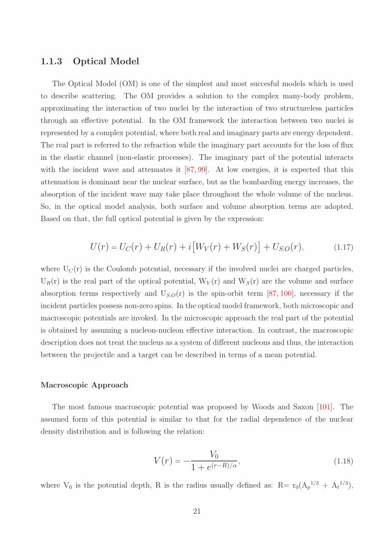
1.1.3 Optical Model

The Optical Model (OM) is one of the simplest and most succesful models which is used

to describe scattering. The OM provides a solution to the complex many-body problem,

approximating the interaction of two nuclei by the interaction of two structureless particles

through an effective potential. In the OM framework the interaction between two nuclei is

represented by a complex potential, where both real and imaginary parts are energy dependent.

The real part is referred to the refraction while the imaginary part accounts for the loss of flux

in the elastic channel (non-elastic processes). The imaginary part of the potential interacts

with the incident wave and attenuates it [87, 99]. At low energies, it is expected that this

attenuation is dominant near the nuclear surface, but as the bombarding energy increases, the

absorption of the incident wave may take place throughout the whole volume of the nucleus.

So, in the optical model analysis, both surface and volume absorption terms are adopted.

Based on that, the full optical potential is given by the expression:

U(r) = UC(r) + UR(r) + i[WV (r) +WS(r)

]+ US.O(r), (1.17)

where UC(r) is the Coulomb potential, necessary if the involved nuclei are charged particles,

UR(r) is the real part of the optical potential, WV (r) and WS(r) are the volume and surface

absorption terms respectively and US.O(r) is the spin-orbit term [87, 100], necessary if the

incident particles possess non-zero spins. In the optical model framework, both microscopic and

macroscopic potentials are invoked. In the microscopic approach the real part of the potential

is obtained by assuming a nucleon-nucleon effective interaction. In contrast, the macroscopic

description does not treat the nucleus as a system of different nucleons and thus, the interaction

between the projectile and a target can be described in terms of a mean potential.

Macroscopic Approach

The most famous macroscopic potential was proposed by Woods and Saxon [101]. The

assumed form of this potential is similar to that for the radial dependence of the nuclear

density distribution and is following the relation:

V (r) =− V0

1 + e(r−R)/α, (1.18)

where V0 is the potential depth, R is the radius usually defined as: R= r0(Ap1/3 + At

1/3),

21

where Ap and At are the mass numbers of the projectile and the target respectively and

α is the diffuseness which describes the decreasing rate of the potential [100]. The optical

potential parameters are usually determined by fitting elastic scattering angular distribution

data. However, at this point we would like to stress out the well-known problem of potential

ambiguities [102–106]. In this, different families of potentials can provide equivalent fits to the

data. To overcome this problem, one has to determine the radial region of sensitivity, where

the nuclear potential can be well and uniquely determined. In order to determine the so called

sensitive radius, the Crossing Point [77,103,107–109] and the Notch Perturbation [77,110–112]

methods are introduced. Below, are presented briefly the main features of each method.

The crossing point method is applied both on the real and the imaginary part of the optical

potential and we will assume that they are both described by Woods-Saxon form factors.

Working separately for the real and the imaginary part, we are changing manually in small

steps the values of the diffuseness αv and we are fitting to the data the depth V0 and the radius

Rv. Then, for the sets (V0,Rv,αv) with the best x2 values, we calculate the potential through

the expression 1.18 and we plot these values as a function of radius r. These potential families

cross each other at a specific radial point x corresponding to the sensitive radius where the

optical potential can be uniquely determined. The Notch Perturbation method is based on the

introduction of a localized perturbation (notch) into the real or imaginary part of the optical

potential at a given radius r, and the observation of the effect of such a perturbation on the

predicted cross sections as the perturbation is moved systematically across the potential. It

is expected that at the radial region where the calculation is very sensitive to the potential

parameters, the perturbation will strongly affect the calculated cross sections, while away from

that region, the impact on the calculated cross sections will be unimportant.

Microscopic Approach

In the microscopic description of the optical potential, the real part of the optical potential

is usually obtained in a double folding model, by using an effective nucleon-nucleon (NN)

interaction folded over matter densities of projectile and the target [113,114]. In this respect,

the potential can be written as:

U(~R) =

∫

d~r1

∫

d~r2ρp(~r1)ρt(~r2)u( ~r12), (1.19)

where ρi, i=(p,t), are the density distributions of the projectile and the target, R is the distance

22

Figure 1.2: Coordinates used in the folding procedure.

between the center of mass of the interacting nuclei and u(r12) is the effective NN interaction.

In principle, the effective interaction has the form [113, 114]:

u(r12) = u00 + u01τ1 · τ2 + u10σ1 · σ2 + u11σ1 · σ2τ1 · τ2, (1.20)

where σ and τ are the Pauli matrices for spin and isospin respectively. The M3Y effective

interaction [113, 115] is the oldest and the most popular interaction which is widely and suc-

cessfully used in elastic scattering and other reactions. In the M3Y approach the first term of

Equation 1.20 is given as:

u00(r, E) =[

7999e−4r

4r− 2134

e−2.5r

2.5r

]

MeV . (1.21)

It is well-established, that the wave function of N identical fermions has to be antisymmet-

ric. However, the term that describes the effective interaction between two nearby nucleons

in the same nucleus is not antisymmetric. To correct that, an additional correction term was

added to the relation above and the effective interaction is given by the following expres-

sion [114]:

u00(r) =

[

7999e−4r

4r− 2134

e−2.5r

2.5r− 276

(

1− 0.005E

A

)

δ(r)

]

MeV , (1.22)

23

with E and A being the energy and the mass number of the projectile respectively. It should

be noted that the M3Y interaction is density independent. Therefore, it is used only in a

short density range approximately the 1/3 of the density of a normal nuclear matter [113]. In

a more realistic analysis, it is necessary to include a density dependent interaction, like the

following [114]:

uDD00 (r, ρ, E) = u00(r)f(ρ, E), (1.23)

where u00(r) is the original M3Y interaction and f (ρ,E) is a function following the form:

f(ρ, E) = C(E)[1 + α(E)e−β(E)ρ

], (1.24)

with ρ being the density of nuclear matter and C(E), α(E) and ρ(E) being energy dependent

parameters. This interaction is known as DDM3Y interaction (Density Dependent M3Y). A

specific parametrization for the function f (ρ,E) was introduced in Refs. [116, 117]

f(ρ) = C[1− αρβ

]. (1.25)

This is called BDM3Y interaction and by replacing this term in Equation 1.19, the overall

potential can be written as:

U(~R) =

∫

d~r1

∫

d~r2ρp(~r1)ρt(~r2)u00(r)

[

C(1− αρβ

)]

. (1.26)

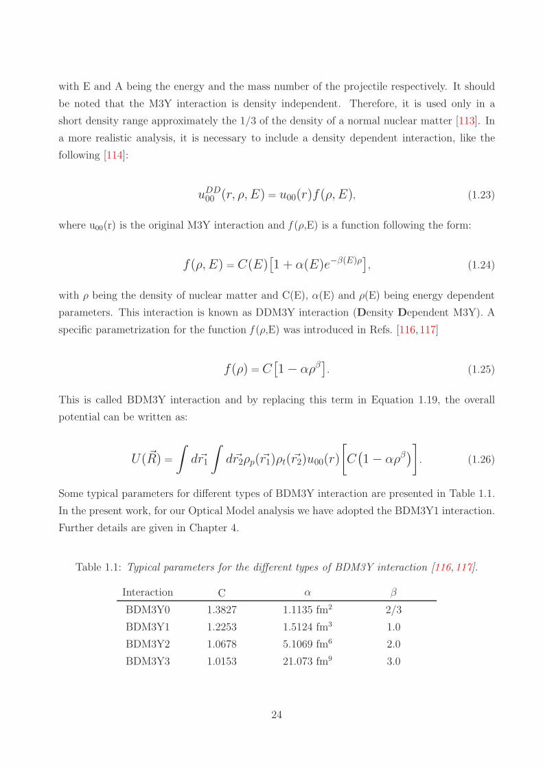
Some typical parameters for different types of BDM3Y interaction are presented in Table 1.1.

In the present work, for our Optical Model analysis we have adopted the BDM3Y1 interaction.

Further details are given in Chapter 4.

Table 1.1: Typical parameters for the different types of BDM3Y interaction [116,117].

Interaction C α β

BDM3Y0 1.3827 1.1135 fm2 2/3

BDM3Y1 1.2253 1.5124 fm3 1.0

BDM3Y2 1.0678 5.1069 fm6 2.0

BDM3Y3 1.0153 21.073 fm9 3.0

24

1.1.4 Threshold Anomaly and Dispersion Relations

As it was already mentioned, both real and imaginary part of the optical potential are

energy dependent. At energies well above the Coulomb barrier, the energy evolution of the

optical potential is almost energy independent but approaching the vicinity of the Coulomb

barrier, this independence no longer holds. The optical model analysis for elastic scattering

data for the 16O + 208Pb [1] and 32S + 40Ca [2] showed that the imaginary potential decreases

rapidly at barrier, while the real potential presents a localized peak. That behavior was named

Threshold Anomaly (TA). The real part of the optical potential can be written as:

V (E) = V0 +∆V (E), (1.27)

where V0 is an energy independent term and ∆V(E) is called dynamic polarization poten-

tial and reflects the effect on V(E) of couplings to non-elastic processes [3–5]. This term is

connected with the imaginary part through a dispersion relation. The dispersion relation is

similar to that appearing in optics for the interaction between the electric field and a dielectric

material, connecting the absorption coefficient with the refraction index [118–120]. In our case,

the dispersive term is given by the expression [5]:

∆V (E) =P

π

∫ ∞

−∞

W (E ′)

E ′ − EdE ′

, (1.28)

where P is the principle value and W(E) is the function that describes the energy dependence

of the imaginary potential. The subtracted version of Equation 1.28 which was first suggested

by Satchler [5], leads to the following expression:

∆V (E)−∆V (ES) = (E − ES)P

π

∫W (E ′)

(E ′ − ES) ∗ (E ′ − E)dE ′, (1.29)

where ES is a reference energy. In order to calculate this quantity, the linear segment model [5]

is adopted where in this approach, the function W(E) is described by three linear segments (or

more) as it is shown in Figure 1.3. The result for the ∆V(E) is given by the following relation:

25

π∆V (E) =W0

(ǫa ln |ǫa| − ǫb ln |ǫb|

)+ (W1 −W0)

(ǫ′b ln |ǫ′b| − ǫ′c ln |ǫ′c|

)−

W1

(ǫ′′c ln |ǫ′′c | − ǫ′′m ln |ǫ′′m|

)+W1

(η ln η − (η + 1) ln (η + 1)

),

(1.30)

where W0,W1≥0 and

ǫi =E − Ei

∆0, ǫ′i =

E − Ei

∆1, ǫ′′i =

E − Ei

∆m, η =

∆1

∆m. (1.31)

Figure 1.3: The linear schematic model for W(E), consisting of three straight-line segments. Figurefrom Ref. [4].

1.2 Reaction Mechanisms

As it was already mentioned above, during a nuclear collision different types of reactions

can take place. Besides the elastic scattering, where the nuclei at the entrance and the exit

channel are the same, we can distinguish two types of nuclear reactions:

Direct reactions and compound nucleus reactions. The main features for each mecha-

nisms are presented below.

26

Figure 1.4: Classical description of the heavy ion collisions, showing the trajectories corresponding todifferent values of the impact parameter b [87].

1.2.1 Direct Reactions

The term “direct reaction” characterizes a reaction mechanism which occurs fast and pro-

ceeds directly from the initial to the final state without forming an intermediate compound

state [8,99]. The time of interaction between the incident and the target nucleus is very short

(∆t≈10−22s) compared to the life time of the corresponding compound nucleus (t≈10−17s). In

a classical description of the heavy ion collisions via the impact parameter b [87, 121] (Figure

1.4), direct reactions correspond to trajectories with larger impact parameters than in the case

of compound nucleus reactions. The most interesting types of direct reactions are: the strip-

ping reaction, its inverse process, the pickup reaction, the knock-out reaction and the breakup

reaction.

• Stripping reactions: In the case of a stripping reaction, when the incident nucleus ap-

proaches the target, a strong interaction takes place between the outer nucleons of the

projectile and the outer nucleons of the target. Thus, there is a possibility for one or

more peripheral nucleons to be detached from the projectile and captured by the target

(Figure 1.5a). Assuming a reaction of the form:

27

α + A −→(α− x

)

︸ ︷︷ ︸

b

+(A+ x

)

︸ ︷︷ ︸

B

(1.32)

the Q-value is given by the expression:

Q =(Mα +MA −Mb −MB

)c2. (1.33)

The binding energy of nucleus B is:

EB =(MA +Mx −MB

)c2 (1.34)

and the separation energy for the removal of the valence particle x from the projectile

nucleus α is given by the expression:

Sx =(Mx +Mb −Mα

)c2. (1.35)

Using Equations 1.34 and 1.35, the Q-value for a stripping reaction can be written as:

Q =(− Sx + EB

). (1.36)

• Pickup reactions: The inverse process of the reaction mechanism described above is

known as pickup reaction. During a peripheral collision between two nuclei, a cluster

of nucleons (or a single nucleon) is transferred from the target to the projectile (Figure

1.5b). Assuming a reaction of the form:

α + A −→(α + x

)

︸ ︷︷ ︸

b

+(A− x

)

︸ ︷︷ ︸

B

(1.37)

the Q-value is evaluated through the relation 1.33. The binding energy of nucleus b is

given as:

Eb =(Mα +Mx −Mb

)c2 (1.38)

and the separation energy for the removal of the valence particle x from the target nucleus

A is given by the expression:

28

Sx =(Mx +MB −MA

)c2. (1.39)

Using Equations 1.38 and 1.39, the Q-value for a pickup reaction can be written as:

Q =(− Sx + Eb

). (1.40)

• Knock-out reactions: In a knock-out reaction [121], during a high energy collision one

or more nucleons are knocked-out from the target by the projectile and both projectile

and nucleons continue moving freely (Figure 1.5c). On the other hand, in a pickup

reaction, one or more nucleons of the target are peaked up by the projectile. The form

of a knock-out reaction is:

α +A −→ α + x+(A− x

)

︸ ︷︷ ︸

B

(1.41)

with a Q-value given as:

Q = −Sx, (1.42)

where Sx is the separation energy for the removal of the valence particle x from the target

nucleus A. These reactions are also known as quasi-free scattering because they permit

a description of the whole procedure as an interaction between the target and one of the

outer nucleons of the projectile (Figure 1.5c).

• Breakup reactions: In a breakup reaction, the projectile nucleus which is usually a weakly

bound one (e.g. 6,7,11Li, 7,9Be) breaks into two or more fragments, due to the Coulomb

and/or nuclear interactions with the target nucleus [8]. The breakup process can be

further classified in direct and sequential breakup. In the first case, the weakly bound

projectiles breaks immediately during the interaction with the target nucleus, while in

the later the projectile is formed in a resonant state and subsequently decays into two

or more fragments [122]. Considering a breakup reaction as the following one:

α + A −→ b+ x+ A, (1.43)

the smallest value of the modulus of Q-value for such a process is:

29

Figure 1.5: Schematic representation of the direct nuclear reaction mechanisms.

30

Q = Eα, (1.44)

with Eα being the binding energy of the projectile nucleus α.

The description of a breakup reaction, is usually performed in the CDCC framework de-

tails of which were presented in Subsection 1.1.2. The rest of the direct reactions, may be

described in the Distorted Wave Born Approximation (DWBA) framework, details of which

are presented below.

Distorted Wave Born Approximation

As it was already mentioned in Subsection 1.1.1, in order to describe the scattering of the

projectile by the target [85], we have to solve the Schrodinger equation:

[

− ~2

2µ∇2 + V (~r)

]

Ψ(~r) = EΨ(~r), (1.45)

where µ is the reduced mass, E is the energy in the center of mass frame and V(~r) the potential

that describes the interaction between the projectile and the target. If we define

U(~r) =2µ

~2V (~r) (1.46)

equation 1.45 can be written as:

(

∇2 + k2)

Ψ(~r) = U(~r)Ψ(~r). (1.47)

The solution of the homogeneous equation (right-hand side of Equation 1.47 equals to zero)

corresponds to a plane wave and is given by the expression:

Xk(~r) = Ae(~k·~r)

, (1.48)

and so the general solution of Equation 1.47 is:

Ψk(~r) = e(~k·~r) +

∫

d3r′G(~r, ~r′)U(~r′)Ψk(~r′), (1.49)

31

where A was set equal to 1 and G(~r,~r′) being the Green’s function defined as: [87]

G(~r, ~r′) =− 1

4π

eik|~r−~r′|∣∣∣~r − ~r′

∣∣∣

. (1.50)

In order to determine the scattering amplitude and thus the differential cross section, we

need to know the behavior of Ψk(~r) at large distances from the target. The Green’s function

behaves asymptotically as:

G(~r, ~r′) =− 1

4π

eikr

re−i~k′·~r′, r → ∞ (1.51)

where it was assumed that: ~k′= k r. So, the wave function defined by Equation 1.49 has the

asymptotic form:

Ψk(~r) = e(~k·~r) − 1

4π

eikr

r

∫

d3r′e−i~k′·~r′U(~r′)Ψk(~r′), r → ∞. (1.52)

Identifying the scattering amplitude as the coefficient of the outgoing wave, we obtain an

integral expression for the scattering amplitude:

f(θ, φ) =− 1

4π

∫

d3r′e−i~k′·~r′U(~r′)Ψk(~r′). (1.53)

Despite the simple form of the Equation 1.53, we still cannot calculate the scattering amplitude

since the integral form contains the unknown wave function Ψk(~r′), but if the potential U(~r) is

weak, the amplitude of Ψk(~r′) is small and the unknown wave function can be replaced by the

plane wave ei~k·~r. This is called First Order Born Approximation. That leads to the expression

of the scattering amplitude where everything is known [121]:

fBA(θ, φ) = − 1

4π

∫

d3r′e−i~k′·~r′U(~r′)ei~k′·~r′

. (1.54)

Moving one step forward, we can assume that the potential U(~r) can be written as U(~r)=

U0(~r) + U1(~r) and for U0(~r) the exact solution can be found by solving the equation [121]:

(

∇2 + k2)

X0k(~r) = U0(~r)X0k(~r). (1.55)

32

So, the plane waves of Equation 1.48 are replaced with the solutions of the above equation and

are called distorted waves X(±)0k (~r). The X

(+)0k (~r) corresponds to a plane wave plus an outgoing

scattered wave, while the X(−)0k (~r) corresponds to a plane wave plus an ingoing scattered wave.

Considering all the above, the asymptotic form of the Ψk(~r) can be written as:

Ψk(~r) =X(+)0k (~r)− 1

4π

eikr

r

∫

d3r′X(−)0k′ (

~r′)∗U1(~r′)Ψk(~r′), r → ∞. (1.56)

If the potential U1(~r) is sufficiently weak compared to U0(~r), Ψk(~r′) can be replaced by X(+)0k (~r′).

This approximation is called Distorted Wave Born Approximation (DWBA) and the expres-

sion for the scattering amplitude is [121]:

fDWBA(θ, φ) = f0(θ, φ)−1

4π

∫

d3r′X(−)0k′ (

~r′)∗U1(~r′)X(+)0k (~r′). (1.57)

The entire procedure described above, is referred to the elastic scattering process. In a

more general case the interaction potential can be written by two terms. The U0(~r) is chosen

to describe the elastic scattering, while the U1(~r) describes the interaction responsible for the

direct reaction. In this respect, it is valid to use DWBA for direct reactions if only the elastic

scattering is stronger than any other possible process [121]. Then, the transition amplitude

for the reaction A(a,b)B has the form of:

fDWBAdirect (θ, φ) =− 1

4π

∫

d3rαd3rβX

(−)β (~rβ)

∗⟨b, B | U1 | a, A⟩X(+)

α ( ~rα), (1.58)

where Xα is used to describe the elastic scattering at the entrance channel (α= a + A), while Xβ

is used to describe the elastic scattering at the exit channel (β= b + B). Therefore, transition

amplitudes are strongly dependent on the entrance and exit channel potentials, highlighting

the importance of the elastic scattering measurements which provide the information about

nucleus - nucleus potential. In the present work, the theoretical predictions [123] for the transfer

reactions under consideration were obtained in the DWBA framework via code FRESCO [98].

Details about the calculations are given in Chapter 4.

33

1.2.2 Compound Nucleus Reactions

In a compound nucleus reaction, the projectile and the target are merged forming a com-

pound nucleus in a high excited state. The compound nucleus life time is ≈10−17s (this is the

lifetime at low excitation energies and decreases with the increasing excitation energy). During

that time interval, the excitation energy of the compound system is shared among the nucleons

of which it is consisted until one or more nucleons acquires enough energy to escape [100,121].

The compound nucleus mechanism can be described by the two-stage scheme:

α +A −→ C∗ −→ b+ B∗, (1.59)

where α is the projectile, A is the target, C∗ is the excited compound nucleus and b, B∗ are

the reaction products after the compound nucleus decay. The excited B∗ nucleus will decay

either through particle emission, if the excitation energy is sufficiently large, or through γ,

β decay [121]. The life time of the compound nucleus is very long compared to the time

within the incident particles and the target nucleus interact during a direct reaction. As a

consequence, the compound nucleus B∗ has lost the information of its formation (entrance

channel) and thus, it will decay in various modes irrespective of the formation process. This

is known as Bohr independence hypothesis [100,121,124]. Based on that, the cross section for

the decay of the compound nucleus to a specific channel can be written as:

σαb = σC(E) ∗GCb (E), (1.60)

where σC(E) is the formation cross section of the compound nucleus C∗ from the entrance

channel α + A with energy E, and GCb (E) is the probability for the compound nucleus C∗ to

decay in the b + B channel. Using the Bohr hypohesis, theories like the Hauser-Feshbach [125]

or the Weisskopf-Ewing [126,127] theory have been developed to predict cross sections for the

various decay modes of the compound nucleus. Below are presented briefly the main features

of these theories.

The Hauser-Feshbach theory

Starting from Bohr hypothesis, the cross section for the a particular decay mode from an

initial channel c to a final channel c′ is:

34

σcc′ =∑

J

σJπ(c)ΓJπc′

ΓJπ, (1.61)

where σJπ(c) is the cross section for the compound nucleus formation, ΓJπ is the sum of the

decay widths corresponding to the possible decay modes and the ratioΓJπ

c′

ΓJπ is the probability

for the compound nucleus to decay in a particular channel c′. ΓJπc′ is a fraction of the total

decay width and is connected with the compound nucleus formation cross section, σJπ(c), via

the following relation [87]:

ΓJπc′ ∝ gc′k

2c′σJπ(c), (1.62)

where kc′ is the wave number of the emitted particle and gc′ is the statistical weight of the

final channel. The cross section for the compound nucleus formation is the sum over all orbital

angular momentum values ℓ and is given by the expression [87]:

σJπ(c) =π

k2(2J + 1)

(2i+ 1) + (2I + 1)

∑

ℓ

Tℓ(c), (1.63)

where Tℓ(c) is the transmission coefficient which we assumed that does not depend on spin

J. The transmission coefficients for the light particle emission are usually determined using

optical model potentials. Using Equations 1.62 and 1.63 we can write the decay width as:

ΓJπc′ ∝ gc′k

2c′π

k2(2J + 1)

(2i+ 1) + (2I + 1)

∑

ℓ′

Tℓ′(c′). (1.64)

In the same way, the sum of all decay widths may be written as:

ΓJπ =∑

c

ΓJπc ∝ gck

2c

π

k2(2J + 1)

(2ic + 1) + (2Ic + 1)

∑

c

∑

ℓ

Tℓ(c). (1.65)

where kc is the wave number of the projectile, gc is the statistical weight of the entrance

channel and ic and Ic are the spin of the target and the projectile respectively. Finally, using

equations 1.61, 1.63, 1.64 and 1.65, the cross section for the transition from channel c to the

final channel c′ is given by the Hauser-Feshbach theory as [87]:

35

σcc′ =π

k2

∑

J

(2J + 1)

(2ic + 1) + (2Ic + 1)

∑

ℓ Tℓ(c)∑

ℓ′ Tℓ′(c′)

∑

c

∑

ℓ Tℓ(c). (1.66)

The Weisskopf-Ewing theory

The Weisskopf-Ewing theory [126,127] is the first statistical model which was used for the

description of the compound nucleus decay. This theory is favored when the available energy

is enough such as to excite the states of the compound nucleus which are very close to each

other and thus cannot be resolved. It is simpler than the Hauser-Feshbach theory, since the

decay widths are treated to be independent of spin J and parity [87]. The cross section for a

particular decay mode from an initial channel c to a final channel c′ is given as:

σcc′ = σ(c)Γc′

Γ. (1.67)

Using Equations 1.64 and 1.65 (without summing over ℓ) the relation above can be written as:

σcc′ = σ(c)gc′k

2c′σ(c

′)∑

c gck2cσ(c)

. (1.68)

If the energy of the emitted particle after the compound nucleus decay is within the energy

range of[Ec′ ,Ec′ + dEc′

], the energy of the residual nucleus will be within the energy range of

[Uc′,Uc′ + dUc′

][87], where

Uc′ = Ecomp. − Bc′ − Ec′, (1.69)

with Ecomp. and B′

c being the compound nucleus energy and the binding energy of the emitted

particle in the compound nucleus respectively. Taking also into account the level density of

the residual nucleus ω(Uc′), Equation 1.68 can be written as:

σcc′dEc′ = σ(c)gc′k

2c′σ(c

′)ω(Uc′)dUc′

∑

c

∫ Emaxc

0 gck2cσ(c)ω(Uc)dUc

. (1.70)

The level density of the residual nucleus of the reaction is obtained usually through the constant

temperature model [128], the Fermi gas model [129], the Gilbert-Cameron model [130]. The

calculations of the cross sections for the possible decay modes of a compound nucleus may be

36

determined by the statistical model codes like CASCADE [131] or PACE2 [132]. In the code

CASCADE, the decay sequence starts with a compound nucleus of a given mass and charge

and excitation energy, while its spin distributions are obtained via fusion cross sections from

a strong-absorption model [131]. Then the relative decay widths for the emitted particles or γ

are calculated and the matrices containing the population of the daughter nuclei as function

of excitation energy and angular momentum are generated. This procedure is repeated until

the excitation energy of the compound system is lower than the particle emission threshold.

One disadvantage of this code is that it cannot provide angular distributions for the emitted

particles or the residual nuclei. In case of the code PACE2, the decay sequence is similar as

for the code CASCADE, but at each de excitation step of the compound nucleus, angular

momentum projections are calculated, which enables to determine the angular distribution of

emitted particles. In the present work, the statistical model calculations were performed with

the code PACE2. Details about these calculations are presented on Chapter 4.

37

38

Chapter 2

Experimental Details

The purpose of the present work is the study of the elastic scattering and the relevant

reaction mechanisms for the system 7Be + 28Si at near barrier energies. The experiment,

proposed by Prof. A. Pakou(University of Ioannina

), was visualized at the Istituto Nazionale

di Fisica Nucleare - Laboratori Nazionali di Legnaro (INFN-LNL) in Italy, at the EXOTIC

facility [133–137] with the collaboration of the EXOTIC group and other contributing research

groups as appear in the last part of this thesis. The experiment included angular distribution

measurements for the various ejectiles, which were performed using the detector array of the

EXOTIC facility, EXPADES [138, 139]. Information regarding the beam line are given in the

following Section, while details for the detection system as well as the electronics of the present

experimental setup are presented in Sections 2.2 and 2.3.

2.1 The EXOTIC facility

EXOTIC is a Radioactive Ion Beam facility (RIB) hosted at LNL in Italy. In the EXOTIC

beam line, the RIBs are produced via the In Flight technique (IF) in inverse kinematics, where

a high intensity primary beam of (100-150)pnA, delivered by the LNL XTU-TANDEM Van

de Graaff accelerator, impinges on a gas target. The gas target is confined in a 50 mm long

cylindrical cell with two Havar foil windows 2.2 µm thick, located at the entrance and the exit

of the cell. The windows tolerance has been tested with an internal gas pressure up to 1.2

bar, while the operating gas pressure at most of the experiments is ∼ 1 bar. Furthermore,

the gas target is usually cooled down with liquid N2 and thus, the gain in the intensity of the

secondary beam may be increased by a factor of ∼ 3, compared with a gas target operated

39

Table 2.1: Characteristics of the available radioactive ion beams produced at the EXOTICfacility [68,140].

Primary beam Gas Target Secondary Beam Intensity (pps)17O 1H 17F 1056Li 3He 8B 1037Li 1H 7Be 1057Li 2H 8Li 10515N 1H 15O 104

at a room temperature (300 K) [137]. A list of the RIBs delivered at the EXOTIC facility is

included in Table 2.1.

A schematic view of the EXOTIC facility is presented in Figure 2.1, where the first element

of the EXOTIC line is the slit set S0, located ∼ 200 mm upstream the gas target, which is

used to control the dimensions of the primary beam spot. The common values for the S0 slits

aperture are ±1.5 mm on X and Y axes. After S0, a quadrupole set (Q1-Q3) is placed ∼200 mm downstream the gas target, ensuring large horizontal and vertical acceptances for the

secondary beam of ∆θ= ±50 mrad and ∆φ= ±65 mrad respectively. A second slit system,

S1, is situated ∼ 1 m upstream the dipole magnet (DM) preventing the scattered ions of

the primary beam from impinging on the dipole walls, while the 30o bending dipole magnet

together with the S2 slit system are used to reduce the beam contaminations. Then, with the

appropriate choice of the electric and magnetic fields in the Wien filter (WF), all the spurious

ions will be deflected and eventually blocked by slit system S3, located 136 mm downstream

the exit of the second quadrupole triplet (Q4-Q6). After the secondary beam is purified, is

directed into the scattering chamber.

The scattering chamber of the EXOTIC facility is a 778 mm diameter cylindrical cell

that hosts a rotating platform with four available positions at ±27o, ±69o, ±111o and ±153o

with respect to the beam direction for mounting the telescopes’ supports. By rotating the

platform, different angular configurations may be achieved depending on the physics case of

each experiment.

2.1.1 The dipole

The operating principle of a dipole is quite simple. Considering a charge particle α, with

mass m, charge q moving with constant velocity ~u perpendicular to a uniform magnetic field

~B, its trajectory will be deflected by the the Lorentz force, ~FL. Thus, the charge particle

40

Figure 2.1: A schematic layout of the EXOTIC beam line - Figure from Ref. [135].

is undergoing acceleration leading its track along the circumference of a circle (Figure 2.2a).

The equations of motion describing the movement of the particle inside the magnetic field are

given by the following expression:

~FL = q~u× ~B = m~u2

ρ

quB = mu2

ρ

Bρ =p

q

(2.1)

where, ρ is the radius of the track and the product Bρ is the magnetic rigidity. The magnetic

rigidity expresses the bending strength of the dipole for a given radius and momentum of the

particle. So, the dipole acts like is a filter on magnetic rigidities.

2.1.2 The Wien filter

The Wien filter is an optical device consisting of perpendicular electric (~E) and magnetic

( ~B) fields. Considering the case of the charge particle mentioned above, by entering inside

41

Figure 2.2: a) A schematic representation for the motion of a charge particle inside the homogeneousmagnetic field of a dipole. b) The operation of the Wien filter for a given ratio E/B.

the Wien filter, the ion will “sense” the Coulomb force ~FC , as well as the Lorentz one ~FL.

The two forces have opposite directions (Figure 2.2b). By adjusting properly the values of the

electric and magnetic fields, each force will compensate each other allowing particles with a

specific velocity to pass through the Wien filter unaffected according to Equation 2.2.

~FL =−~FC

q~u× ~B = −q ~E

uB = E

u =E

B

(2.2)

2.2 Detection systems and electronics

The EXOTIC facility includes the following detections systems: Silicon detectors for monitor-

ing the secondary beam in the beginning of the experiment, to be described in Subsection 2.2.1,

two Parallel Plate Avalance Counters -PPAC detectors [137, 139] for mapping the trajectory

of the secondary beam during the experimental procedure- Subsection 2.2.2- and the detection

multi telescope array EXPADES [138, 139] to be described in Subsection 2.2.3.

42

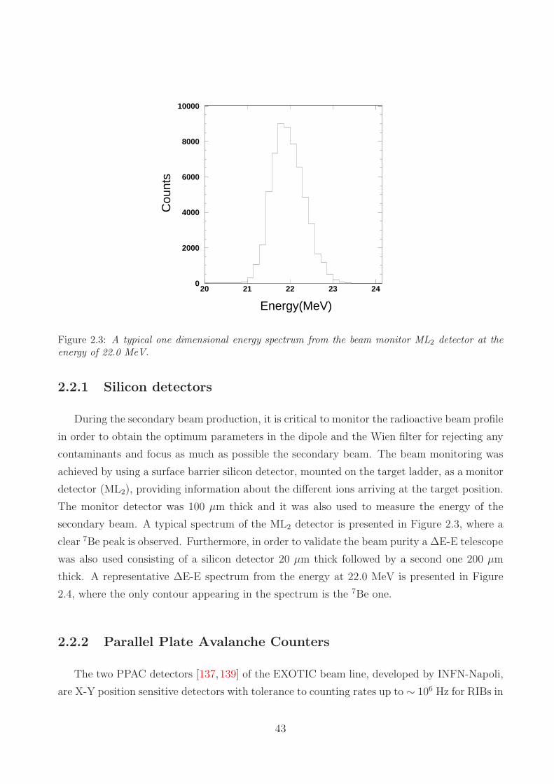
Cou

nts

Energy(MeV)

0

2000

4000

6000

8000

10000

20 21 22 23 24

Figure 2.3: A typical one dimensional energy spectrum from the beam monitor ML2 detector at theenergy of 22.0 MeV.

2.2.1 Silicon detectors

During the secondary beam production, it is critical to monitor the radioactive beam profile

in order to obtain the optimum parameters in the dipole and the Wien filter for rejecting any

contaminants and focus as much as possible the secondary beam. The beam monitoring was

achieved by using a surface barrier silicon detector, mounted on the target ladder, as a monitor

detector (ML2), providing information about the different ions arriving at the target position.

The monitor detector was 100 µm thick and it was also used to measure the energy of the

secondary beam. A typical spectrum of the ML2 detector is presented in Figure 2.3, where a

clear 7Be peak is observed. Furthermore, in order to validate the beam purity a ∆E-E telescope

was also used consisting of a silicon detector 20 µm thick followed by a second one 200 µm

thick. A representative ∆E-E spectrum from the energy at 22.0 MeV is presented in Figure

2.4, where the only contour appearing in the spectrum is the 7Be one.

2.2.2 Parallel Plate Avalanche Counters

The two PPAC detectors [137,139] of the EXOTIC beam line, developed by INFN-Napoli,

are X-Y position sensitive detectors with tolerance to counting rates up to ∼ 106 Hz for RIBs in

43

∆E(C

hann

el)

E(Channel)

0

500

1000

1500

2000

2500

0 1000 2000 3000 4000

Figure 2.4: A typical ∆E-E spectrum at the energy of 22.0 MeV from the telescope mounted on thetarget ladder. It is obvious that the possible beam contaminants were successfully suppressed.

the energy regime of (3-5) MeV/u. The first PPAC (PPACA) is located 909 mm upstream the

secondary target, while the second one (PPACB) is located at the entrance of the scattering

chamber, 365 mm upstream the secondary target. The PPAC detector has an active area of

(62 × 62) mm2 and is usually operated with isobutane (C4H10) at a pressure of 10 to 20 mbar.

Each PPAC consists of a cathode plate between two anodes. The cathode plate is made of

a mylar foil 1.5 µm thick with an extra layer of 30 nm aluminum evaporated on both sides

of the mylar. Each anode consists of 60 wires 20 µm thick with 1 mm spacing from each

other. The two anodes are placed perpendicular to each other ensuring a position resolution

of 1 mm(X) × 1 mm(Y). The anode wires are connected to a 2.3 ns/mm delay line. The

charge collected by the anodes produces a signal travelling towards the delay line (see Figure

2.5). Reaching the delay line, the signal is splitted in two directions (Left-Right or Up-Down)

travelling simultaneously towards the two ends (X1 and X2 or Y1 and Y2). The time interval

that the signal needs to reach each end is measured with a Time to Digital Converter (TDC),

using as a start the signal from the cathode, while the stop signal is provided by each end.

The time difference of the arrival time of the signal between the the two ends of the delay line

is proportional to the position of the particle. Absolute measurements of the position of the

particles are obtained after calibrating the PPAC’s as follows. Almost all the active area of a

PPAC is irradiated by the secondary beam. Thus, by plotting the differences (X1 - X2) or (Y1

44

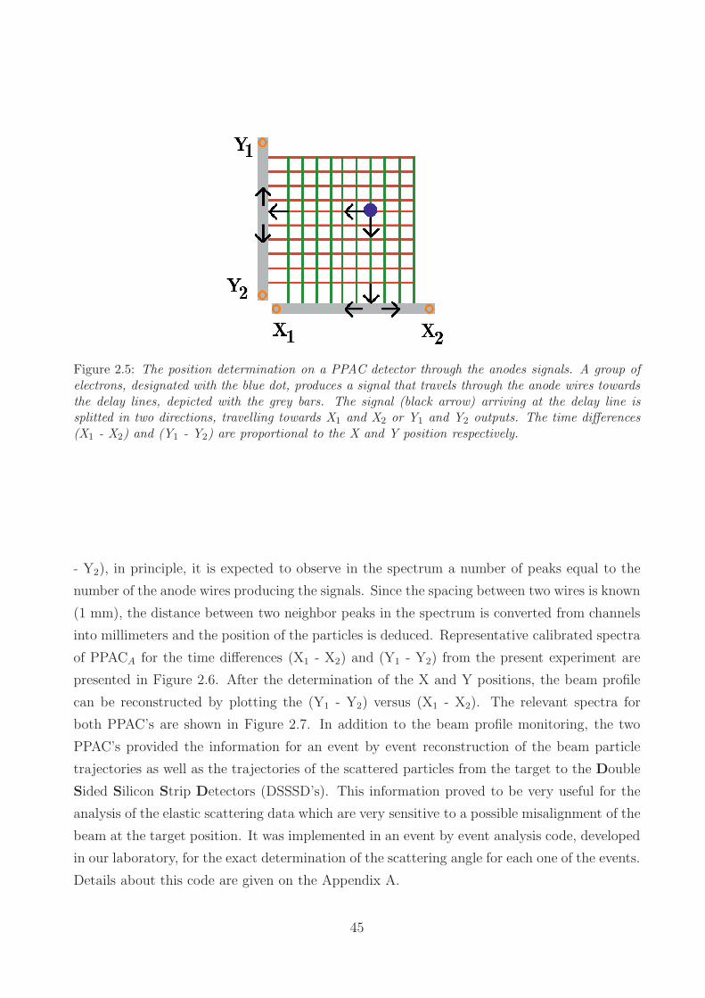
Figure 2.5: The position determination on a PPAC detector through the anodes signals. A group ofelectrons, designated with the blue dot, produces a signal that travels through the anode wires towardsthe delay lines, depicted with the grey bars. The signal (black arrow) arriving at the delay line issplitted in two directions, travelling towards X1 and X2 or Y1 and Y2 outputs. The time differences(X1 - X2) and (Y1 - Y2) are proportional to the X and Y position respectively.

- Y2), in principle, it is expected to observe in the spectrum a number of peaks equal to the

number of the anode wires producing the signals. Since the spacing between two wires is known

(1 mm), the distance between two neighbor peaks in the spectrum is converted from channels

into millimeters and the position of the particles is deduced. Representative calibrated spectra

of PPACA for the time differences (X1 - X2) and (Y1 - Y2) from the present experiment are

presented in Figure 2.6. After the determination of the X and Y positions, the beam profile

can be reconstructed by plotting the (Y1 - Y2) versus (X1 - X2). The relevant spectra for

both PPAC’s are shown in Figure 2.7. In addition to the beam profile monitoring, the two

PPAC’s provided the information for an event by event reconstruction of the beam particle

trajectories as well as the trajectories of the scattered particles from the target to the Double

Sided Silicon Strip Detectors (DSSSD’s). This information proved to be very useful for the

analysis of the elastic scattering data which are very sensitive to a possible misalignment of the

beam at the target position. It was implemented in an event by event analysis code, developed

in our laboratory, for the exact determination of the scattering angle for each one of the events.

Details about this code are given on the Appendix A.

45

Cou

nts

Cou

nts

Position(mm)

a)

b)

0

1000

2000

3000

-20 -10 0 10 20

0

5000

10000

-10 -5 0 5 10

Figure 2.6: a) The determination of X position on PPACA for the 7Be beam at the energy of 22.0MeV. b) The determination of Y position on PPACA for the 7Be beam at the energy of 22.0 MeV.

Y p

ositi

on(m

m)

X position(mm)

a)

b)-20

-10

0

10

20

-40 -20 0 20 40

-20

-10

0

10

20

-40 -20 0 20 40

Figure 2.7: a) The 7Be beam profile as it was recorded on PPACA at the energy of 22.0 MeV. b) The7Be beam profile as it was recorded on PPACB at the energy of 22.0 MeV.

46

2.2.3 Double Sided Silicon Strip Detectors (DSSSD) and the EX-

PADES array

The advent of radioactive beam facilities moved the interest to measurements involving

exotic nuclei especially at near barrier energies, where the direct mechanisms are expected to

be of great importance creating a very interesting field for studies of reaction mechanisms and

channel coupling effects. Since the RIBs are usually produced with lower intensities than the

stable ones, a detector system covering a large solid angle together with high granularity is

required. These features are met in the DSSSD arrays(Double Sided Silicon Strip Detectors

).

A DSSSD is consisted of an n-type silicon layer having implanted p+ silicon strips on the

one side (front) and n− silicon strips on the other side (back) [141,142]. The p+ indicates that

the crystal is highly doped with impurities increasing the population of the holes, while n−

indicates that the crystal is doped with impurities such as there is an excess of free electrons.

In the space between the series of n− strips, thinner p+ silicon strips are implanted for electrical

isolation purposes. A reverse biased voltage is applied over the detector, creating an electric

field throughout the n-type silicon layer that prevents the recombination of the electrons and

holes, leading to the formation of the so called depletion region. When a charged particle

passes through the detector, electron-hole pairs are formed in the depletion region. Then, both

charge carriers are moving in opposite directions producing two coincidence signals. Each strip

is connected to its own amplifier and so, the coincidence signal from a single event is amplified

and through the readout electronics the energy loss of the ion as well as its position in the

detector are determined.

The past few years, a large number of DSSSD arrays like EXPADES [138, 139], GLORIA

[143, 144], MUST2 [145, 146], TIARA [147], LASSA [148], HiRA [149] and LEDA [150] were

developed dedicated to measurements with stable or radioactive beams. In the present study

the DSSSD array of the EXOTIC facility, EXPADES (EXotic PArticle DEtection System)

was used. EXPADES is a detector array of eight telescopes, each one comprised by two

DSSSD’s with the possibility to use also an ionization chamber (IC). In the present experiment

the IC part was not available therefore, the main focus will be given on the description of the

DSSSD’s. The ∆E stage of the telescopes is a DSSSD (45-60)µm thick detector, while the E

stage is a DSSSD ∼ 300 µm thick detector. The DSSSD’s have active areas of (64 × 64) mm2

with 32 strips per side. The y strips, providing the information of Y position, are implanted

on the front side of the detector and are orthogonally oriented with respect to the the x strips

on the back side, providing the information of X position. Thus, pixels of (2 × 2) mm2 are

47

defined. The signal readout electronics for the ∆E stage of the telescopes are different from

those for the E one as explained in [138,139]. A short description for both types of electronics

is given below.

At the ∆E stage of the detector, both x and y strips were short-circuited two-by-two in

order to reduce the cost as well as complexity of the signal handling. The ∆E electronics

readout were developed by INFN-Milano and include a charge sensitive preamplifier and an

amplifier module called MEGAMP [151]. The preamplifier module has 16 input channels and

it generates 16 differential output signals, fed as an input to the MEGAMP. The MEGAMP

amplifier has 16 input channels where each one provides information both for energy and time.

The energy information is provided from a spectroscopy amplifier. The signal is amplified

properly by means of a 2-bit coarse gain stage followed by an 8-bit fine gain stage and then

is sent to the ADC module. The time information is provided using two Constant Fraction

Discriminators (CFDs) and a Time to Analog Converter (TAC). The CFDs provide an output

signal at 30% and 80% of the signal leading edge. The 30% CFD output provides the START

signal to the TAC unit, while the STOP signal is provided either by the 80% CFD output or

an external signal. Using as STOP the 80% CFD signal the TAC unit provides a pulse shape

information, while an external signal may be used for Time Of Flight (TOF) measurements.

The block diagram for a single channel of the MEGAMP is displayed in Figure 2.8.

Regarding the E stage, the readout electronics include 32-channel ASIC chips (VA and TA)

installed on a board (VA-TA board), designed by INFN-Padova, for each side of the detector

(front and back). The development of the electronics was based on similar work described

in Refs. [149, 152]. The VA chip is employed for the treatment of the energy signal and the

TA chip for the treatment of the logic signal. The VA chip is consisted of a charge sensitive

preamplifier followed by a slow amplifier and a Sample and Hold unit. In contrast to the

MEGAMP module, the amplification via the VA chip is common for all strips and can be set

at four discrete values allowing a dynamic range for the detector of 30, 52, 90 and 113 MeV.

After the amplification stage, the signals from all the strips are combined into one through

a multiplexer (MUX) and the final signal is sent to the ADC. The TA chip is comprised of

a fast shape unit followed by a discriminator, where its output signal is sent to the Trigger

Supervisor (TSB) which is responsible for the trigger logic. The block diagram for a single

channel of the VA-TA board is illustrated in Figure 2.9. These are in short the main features

of the electronics for the ∆E-E telescopes of the EXOTIC facility. Further details are given in

Ref. [139].

48

Figure 2.8: The block diagram of the MEGAMP amplifier for a single channel - Figure from Ref. [139].

Figure 2.9: The block diagram of the VA-TA board for a single channel - Figure from Ref. [139].

49

2.2.4 The trigger of the experiment

In the previous Subsection, a short description about the EXPADES array and its elec-

tronics was presented. Further on, the main concept of the experimental design is the trigger

of the electronics. The trigger is controlled via the Trigger Supervisor (TSB) board. The

TSB accepts the OR signals of the x and y strips from both stages of the ∆E-E telescopes.

Also, signals from external sources, usually from PPAC’s, are fed as an input to the TSB.

The TSB board includes four different stages: The first stage receives the signal from all the

DSSSD’s. The second stage receives the signal from the external sources together with the

output of the first stage. In the third stage, the output of the second stage is used to create

further logic and in the final stage, the so called Master Trigger signal for the chain of the

electronics is generated. In our case, the Master Trigger of the experiment was created as the

logical AND between the OR signal of the ∆E stage of the telescopes and the signal from the

cathode of PPACA. Under normal circumstances, the PPACA signal precedes the signal from

the DSSSD’s. Thus, the signal from the cathode of PPACA was delayed by 200 ns, such as the

two signals were overlapped within a certain time window.

2.3 Experimental setup and procedure

In the present experiment, six telescopes from the EXPADES array were used with the

following standard configuration. The forward telescopes T1 and T6 were set at ±27o, the

middle telescopes T2 and T5 at ±69o and the backward ones T3 and T4 at ±111o, covering

the following angular ranges: ∼ (13o to 41o) and ∼ (14o to 40o) for the forward telescopes, ∼(54o to 85o) for the middle telescopes and ∼ (96o to 126o) for the backward telescopes. The

telescopes were set at symmetrical positions to balance any beam divergence and to improve

the statistics of the measurement. A schematic view of the experimental setup is displayed in

Figure 2.10, while a photo with the telescopes mounted in the scattering chamber appears in

Figure 2.11. In the center of the scattering chamber, a target ladder was installed with several

available positions (Figure 2.12). In the present experiment, three kinds of targets were used.

For the main measurement, two 28Si targets 0.4 mg/cm2 and 0.6 mg/cm2 thick were used, the

second one for the measurement at the energy of 17.2 MeV. In addition, the thick silicon and

a 208Pb target (2 mg/cm2) were used at the energies of 9.0 and 22.0 MeV respectively for the

solid angle determination, since the scattering at such energies is of Rutherford type.

For the needs of the present study, the 7Be secondary radioactive beam was produced by

50

Figure 2.10: Schematic view of the experimental setup which includes 6 of the 8 modules of theEXOTIC array EXPADES [138, 139]. Each module includes two DSSSD’s as explained in the text.Telescopes T1 and T6 were set at ±27o, T2 and T5 at ±69o and T3 and T4 at ±111o, covering thefollowing angular ranges: ∼ 13o to 41o and ∼ 14o to 40o for the forward telescopes, ∼ 54o to 85o forthe middle telescopes and ∼ 96o to 126o for the backward telescopes.

means of the 1H(7Li,7Be)n reaction. The 7Li primary beam with an intensity of 150 pnA,

produced at three energies namely 26, 31 and 33 MeV, impinged on a H2 gas primary target

at a pressure of 1 bar and a temperature of 93 K corresponding to an effective thickness of

1.35 mg/cm2. The 7Be beam was produced at five near barrier energies namely 9.0, 13.2, 17.2,

19.8 and 22.0 MeV, the highest three being obtained by re-tuning the primary beam while

the lowest two using an 27Al degrader at the energies of 19.8 and 17.2 MeV. After the gas

target, the 7Be beam was directed into a series of optical elements, slits sets and collimators

placed along the beam line, allowing the separation of 7Be from the scattered 7Li ions and

possible 4He contaminations from the 1H(7Li,4He)4He reaction, as it was explained in Section

2.1. In the present experiment, the average 7Be beam intensity was ∼ 5 x 104 pps on the target

position.

51

Figure 2.11: A photo of the detectors’ arrangement inside the scattering chamber.

Table 2.2: The information regarding the telescopes arrangement inside the scattering chamber.The first column indicates the telescope identity, the second one includes the distances of eachtelescope with respect to the target position, the third column includes the mean angle of eachtelescope, while the last one the angular range covered by each telescope.

Telescope IDDistance from the

target (mm)Mean angle (deg) Angular range (deg)

T1 123.0 27.0 13.0 - 41.0T2 111.0 69.0 53.5 - 84.5T3 115.0 111.0 94.8 - 127.2T4 106.0 111.0 96.1 - 126.0T5 111.0 69.0 53.5 - 84.5T6 134.0 27.0 14.2 - 39.8

52

Figure 2.12: Schematic representation of the target ladder used in the present experiment.

53

54

Chapter 3

Data Reduction

In order to deduce the optical potential and map its energy evolution, elastic scattering

angular distribution data were determined at various near barrier energies, namely 13.2, 17.2,

19.8 and 22.0 MeV(E/VC.b.= 1.14, 1.48, 1.71, 1.90

). Further on, the degree of competition

between direct and the compound nucleus mechanisms was sought by considering the 3He and4He reaction products. For that, experimental angular distributions together with direct and

compound nucleus calculations were used, as the tool for disentangling the various mechanisms.

In the following, details about the data reduction are presented, leading to differential cross

sections either for the elastically scattered 7Be ions(Section 3.2

)or the 3,4He reaction products

(Section 3.3

).

3.1 Energy calibration

For the identification of the reaction products, especially in the present case were the

elastically scattered ions stop in the first stage of the telescope, an accurate energy calibration of

the detectors is necessary. In order to span the whole dynamical range of them, the calibration

was performed by using a pulser in combination with a triple alpha source (239Pu, 241Am,244Cm). The pulser generator was calibrated through the alpha source and the detectors

through the pulser. Thus, the accuracy of the calibration was extended in a wide energy

range. Representative spectra for the calibration of one strip of the ∆E stage of telescope T6

are displayed in Figure 3.1.

55

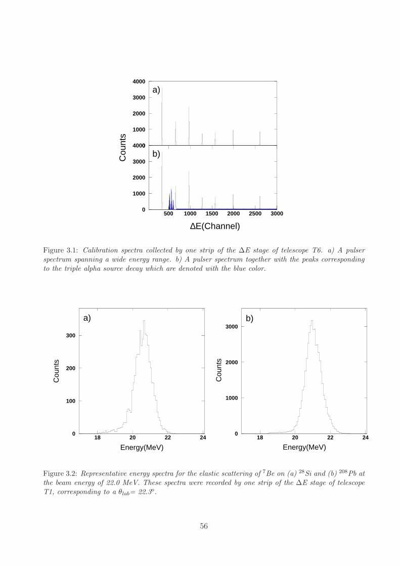
Cou

nts

∆E(Channel)

a)

b)0

1000

2000

3000

4000

500 1000 1500 2000 2500 3000

0

1000

2000

3000

4000

500 1000 1500 2000 2500 3000

Figure 3.1: Calibration spectra collected by one strip of the ∆E stage of telescope T6. a) A pulserspectrum spanning a wide energy range. b) A pulser spectrum together with the peaks correspondingto the triple alpha source decay which are denoted with the blue color.

Cou

nts

Energy(MeV)

a)

0

100

200

300

18 20 22 24

Cou

nts

Energy(MeV)

b)

0

1000

2000

3000

18 20 22 24

Figure 3.2: Representative energy spectra for the elastic scattering of 7Be on (a) 28Si and (b) 208Pb atthe beam energy of 22.0 MeV. These spectra were recorded by one strip of the ∆E stage of telescopeT1, corresponding to a θlab= 22.3o.

56

3.2 Determination of the elastic scattering cross sec-

tions

The elastically scattered 7Be ions were stopped in the first stage of the telescope and were

identified taking into account the kinematics of the colliding ions and the energy loss, using

the programs NRV [153] and LISE++ [154]. A typical one dimensional energy spectrum from

a telescope set at forward angles is shown in the left panel of Figure 3.2. As it is seen, the peak

is well pronounced and no other events are present near by. This is because, the other light

reaction products did not stop in this detector but punched through, therefore leaving very

little energy in it. At this point it should be mentioned that the data in the present analysis

refer to quasi - elastic scattering, since excitations to the 1/2− state of 7Be (0.429 MeV) or the

2+ state of 28Si (1.779 MeV) could not be resolved from pure elastic scattering events.

The reduction of the quasi - elastic scattering events was performed by means of an

event by event code, developed in our laboratory, using the data analysis package ROOT [155].

Details of this code will be given in Appendix A. Briefly we can refer on that as following.

Experimentally the coordinates for each beam particle are determined in two places via the

information collected by the two PPAC’s. This information is implemented in our code and

via analytic geometry, the beam particle trajectories are reconstructed. In this respect, the

reaction position on the target is defined for each event. Subsequently, the DSSSD telescopes

provide the position of each elastically scattered particle, since each event is detected in a

unique pixel of the detector. By using the coordinates of the reaction position on the target

together with the coordinates of the events detected in the DSSSD’s, the scattering angle for

each event can be determined.

Data concerning both the quasi - elastic scattering of 7Be on 28Si and 208Pb were treated

in an event by event framework. Events with the same angle or with an angle inside an angular

range corresponding to a particular strip of each EXPADES detector were summed up. The

so performed event by event analysis, reported in Ref. [156], improved greatly our preliminary

strip or/and pixel analysis reported previously in [157]. The ratios σ/σSiRuth were deduced

according to the following expression:

Ratio ≡σ

σSiRuth

=NSi

NPb∗K (3.1)

where NSi and NPb are the event by event counts corresponding to every strip collected with

57

the silicon and lead targets respectively and the constant K corresponds to

K =TPbΦPb

TSiΦSi

σPbRuth

σSiRuth

(3.2)

where TSi and TPb are the scattering centers of the silicon and lead targets respectively, ΦSi

and ΦPb are the beam fluxes during the runs with the silicon and lead targets respectively and

σSiRuth and σPb

Ruth are the calculated Rutherford cross sections for the elastic scattering of 7Be on28Si and 208Pb respectively. In case of the 17.2 MeV data, the main quasi - elastic scattering

data were combined with quasi - elastic scattering data at 9.0 MeV where the scattering can

be considered as Rutherford, and not with data from the lead target. Thus, Equations 3.1 and

3.2 were slightly modified, where NPb was replaced with NSi9 and TPb was replaced with TSi,

with NSi9 being the event by event counts corresponding to every strip collected with the silicon

target at 9.0 MeV and TSi are the scattering centers of the silicon target. In this particular

case, Equation 3.2 is reduced to Equation 3.3.

K =ΦPb

ΦSi

σPbRuth

σSiRuth

(3.3)

The constant K is determined assuming that at small scattering angles the ratio σ/σSiRuth

between elastic scattering cross sections and Rutherford cross sections is 1.0. This assumption

is valid only at the lowest energy of 13.2 MeV. For the rest of the energies the ratio was

assumed to be closed to 1, according to the theoretical calculations. As a result, the error

assigned to our data, except systematic errors, is connected solely with the statistical errors

from the measurements with the silicon and lead targets and not with errors due to the beam

flux or the target thickess. The error in the ratio was calculated as:

Σ = ±Ratio ∗

(√1

NSi+

1

NPb

)

(3.4)

The results for the quasi - elastic scattering of 7Be+28Si at the energy of 22.0, 19.8, 17.2 and

13.2 MeV are presented in Figures 3.3, 3.4, 3.5 and 3.6 respectively. Differential cross sections

were determined via weighted means of data, collected by telescopes placed at symmetrical

positions. Weighted mean cross sections, were evaluated through the expression:

58

(Ratio

)

mean=

∑

i

(Ratio

)

i

Σ2i

∑

i

1

Σ2i

(3.5)

and the error in the weighted mean was deduced as:

(Σ)

mean= ±

√√√√√

1∑

i

1

Σ2i

(3.6)

σ/σ R

uth

θc.m.(deg)

10-2

10-1

1

0 20 40 60 80

Figure 3.3: Present angular distribution data for the quasi - elastic scattering of 7Be+28Si at theenergy of 22.0 MeV. Tabulated values of the ratios are given in Appendix C.

59

σ/σ R

uth

θc.m.(deg)

10-2

10-1

1

0 20 40 60 80

Figure 3.4: Same as in Figure 3.3 but for the energy of 19.8 MeV. Tabulated values of the ratios aregiven in Appendix C.

σ/σ R

uth

θc.m.(deg)

10-1

1

0 20 40 60 80

Figure 3.5: Same as in Figure 3.3 but for the energy of 17.2 MeV. Tabulated values of the ratios aregiven in Appendix C.

60

σ/σ R

uth

θc.m.(deg)

10-1

1

0 20 40 60 80

Figure 3.6: Same as in Figure 3.3 but for the energy of 13.2 MeV. Tabulated values of the ratios aregiven in Appendix C.

The quasi - elastic scattering data were treated in an Optical Model and a Continuum

Discretized Coupled Channels (CDCC) framework to be described in Chapter 4.

3.3 Determination of the reaction cross sections

Our reaction analysis refers to the production of 3He and 4He either through a direct or a

compound nucleus process. These light particles were able to pass through the ∆E stage of

the telescopes and thus, they were well-discriminated by the ∆E-E technique (see Appendix

E) as may be seen in Figure 3.7. Light particles with low energy that stopped in the first stage

of the telescopes were retrieved via simulations as it will be described below. The reaction

mechanisms leading to the production of 3He are:

1. Projectile breakup: 7Be → 3He + 4He, Sα= 1.586 MeV and

2. 4He stripping: 28Si(7Be,3He)32S, Qgg= 5.36 MeV

while those leading to the production of 4He are:

61

∆E(M

eV)

E(MeV)

0

2

4

6

8

10

0 5 10 15 20 25

Figure 3.7: A representative ∆E-E correlation plot for telescope T1 at the energy of 22.0 MeV. Thesolid green and red lines represent kinematical simulations for the energy loss of 3He and 4He ions inthe telescope using code LISE++ [154], presenting very good agreement with the data.

1. Projectile breakup: 7Be → 3He + 4He, Sα= 1.586 MeV,

2. 3He stripping: 28Si(7Be,4He)31S, Qgg= 10.89 MeV,

3. 1n stripping: 28Si(7Be,6Be)29Si, Qgg= -2.20 MeV, 6Be → 4He + p + p,

4. 1n pickup: 28Si(7Be,8Be)27Si, Qgg= 1.72 MeV, 8Be → 4He + 4He and

5. Evaporation process after compound nucleus formation.

3.3.1 α - particle production cross sections

The α - particle production data were analyzed via the analysis program PAW [158]. The

α yields were obtained by applying the appropriate energy windows on the two dimensional

∆E-E plots. However, it should be noted that due to the thickness of the ∆E detector, an

62

energy threshold in the detection of the two reaction products was introduced. So, an energy

phase space correction was necessary to be applied for the missing counts. This was achieved

via comparisons of the experimental energy spectra with simulated ones. Simulated spectra

were obtained with the contribution of all processes direct and of compound nucleus origin,

normalized appropriately in a best fit. Compound nucleus energy spectra were produced via

the well known code PACE2(Projection Angular-momentum Coupled Evaporation

)[132].

For α - particles produced via a direct process, that is the neutron pickup channel leading to8Be (4He+4He), its inverse process leading to 6Be (4He+2p), the 3He stripping and the breakup

processes, a Monte Carlo simulation code was developed to describe them. Energy spectra for

most of the processes were generated by the code starting from angular distributions obtained in

the DWBA framework, while for the breakup the angular distributions of the continuum states

were obtained in the CDCC framework. In case of the 3He stripping process, no theoretical

calculation was performed due to the lack of the appropriate spectroscopic factors(see Section

4.2). However, for the rest of the processes, tests adopting either specific angular distributions

or isotropic ones did not affect the result for the energy spectra. Therefore, in this particular

case, the simulations were performed with the assumption of an isotropic distribution. Details

regarding the simulation code are given in Appendix B, while as an example, the main features

of the code for the simulation of the neutron stripping process are given below.

In order to construct the alpha energy spectra from the decay of 6Be, the energy and the

momentum of α particles in the laboratory frame are necessary. In this respect, the simulation

code is organized in three steps: In the first step, a theoretical angular distribution for the

1n stripping process, obtained in the DWBA framework using code FRESCO [98], was fed

as an input to the code. Then, the emission angle θc.m. of the 6Be in the center-of-mass

(c.m.) frame was randomly generated, and by using the theoretical angular distribution of6Be as a constrain, we evaluated the frequency of each θc.m. to be observed. Subsequently,

for each emission angle, the momentum modulus in the c.m. frame, Pc.m., was calculated and

subsequently the pairs(θc.m., Pc.m.

)were transformed in the laboratory reference system to

be used in the final step of the code. In the second step, the breakup procedure takes part

in the 6Be rest frame and the 6Be nucleus breaks into an α particle and two protons. The α

particle and one of the protons are emitted with randomly specified energies and momenta and

the third fragment acquires energy and momentum fulfiling the conservations laws of energy

and momentum at the rest frame of 6Be. In the final step, following the prescription of Olimov

et al. [159], by applying a Galilean transformation and an axes rotation, the alpha energy

spectra from the rest frame of 6Be are transformed to the laboratory frame. The same or

similar method was followed for the rest of the direct processes and the final energy spectrum

63

was obtained by summing the four energy spectra normalized to the calculated cross sections.

Finally, direct and the compound nucleus spectra were summed using various assumptions

for the ratio direct to compound nucleus contributions until the best fit to the experimental

data was obtained. Comparisons between experimental and simulated alpha energy spectra(∆E+E

)are shown in Figure 3.8, while the procedure described above is demonstrated in

Figure 3.9 for two representative spectra.

The integrated 4He yields for each strip, after corrections for missing counts (by comparing

experimental and simulated energy spectra), were transformed to differential cross sections in

the laboratory reference system via the following relation:

dσ

dΩ=

Nα

NPb∗K ′ (3.7)

where Nα is the 4He yield for each strip, NPb are the counts for each strip collected from 7Be

quasi - elastic scattering to the lead target and the constant K′ corresponds to

K ′ = K ∗ σSiRuth (3.8)

with K being a constant determined by the quasi - elastic scattering data as it was described

in Section 3.2 and σSiRuth is the calculated Rutherford cross section in the laboratory reference

system for the elastic scattering of 7Be on 28Si. The results of the analysis are presented in

Figure 3.10 and they are also reported in Ref. [160].

3.3.2 3He production cross sections

The 3He particles are produced through direct processes as it was stated above, by breakup

and 4He-stripping. In the same spirit as for the α particle production, missing counts due

to the energy threshold introduced by ∆E detector were estimated via comparisons of the

experimental with the simulated spectra produced by our Monte Carlo code. The results of the

simulations are presented in Figure 3.11. After correcting for missing counts, the integrated 3He

yields for each strip were transformed to differential cross sections in the laboratory reference

system via the Equation 3.7, where Nα was replaced with N3He, with the second being the 3He

yield corresponding to every strip. The angular distributions for the 3He particle production

are shown in Figure 3.12.

Looking at Figure 3.12, it is obvious that the 3He particle angular distributions are forward

64

a)

Cou

nts/

MeV b)

Energy (MeV)

c)

0

50

100

150

0 5 10 15 20 25

0

50

100

0 5 10 15 20 25

0

10

0 5 10 15 20 25

Figure 3.8: Alpha energy spectra(∆E+E

)collected with telescope T1 at three energies a) 22.0 MeV,

b) 19.8 and c) 13.2 MeV. The green solid line represents the simulated spectrum taking into accountboth direct and compound nucleus mechanisms.

65

a) Total3He transferPACE2n-stripping (x5)n-pickupBreakup (x5)

Data

Cou

nts/

MeV

Energy (MeV)

b)Total3He transferPACE2n-stripping (x5)n-pickupBreakup (x5)

Data0

50

100

150

0 5 10 15 20 25

0

10

20

30

40

0 5 10 15 20 25

Figure 3.9: Decomposition of the simulated alpha energy spectra at the energy of 22.0 MeV for tele-scopes (a) T1 and (b) T2 due to compound nucleus process, designated with the dotted black line, anddirect processes as follows: The dashed red line indicates the α spectrum due to 3He stripping, thedashed blue line due to breakup, the dotted-dashed magenta line due to neutron stripping and the solidyellow line due to neutron pickup. The multiplication factors are arbitrary values for the purpose ofpresenting the different processes only.

66

a)

(dσ/

dΩ) la

b(m

b/sr

)

b)

θlab(deg)

c)

10

10 2

0 20 40 60 80 100 120 140

10

10 2

0 20 40 60 80 100 120 140

1

10

10 2

0 20 40 60 80 100 120 140

Figure 3.10: Present angular distribution data for the 4He particle production at the energies of a)22.0 MeV, b) 19.8 MeV and c) 13.2 MeV. Tabulated values of the differential cross sections are givenin Appendix C.

67

a)

Cou

nts/

MeV

b)

Energy (MeV)

c)

0

20

40

0 5 10 15 20

0

20

0 5 10 15 20

0

2

0 5 10 15 20

Figure 3.11: 3He energy spectra collected with telescope T1 at three energies a) 22.0 MeV, b) 19.8 andc) 13.2 MeV. The red solid line represents the simulated spectrum taking into account 4He transferand breakup processes.

68

a)

(dσ/

dΩ) la

b(m

b/sr

)

b)

θlab(deg)

c)

1

10

10 2

0 10 20 30 40 50 60 70 80 90

1

10

10 2

0 10 20 30 40 50 60 70 80 90

1

10

10 2

0 10 20 30 40 50 60 70 80 90

Figure 3.12: Present angular distribution data for the 3He particle production at the energy of a) 22.0MeV, b) 19.8 MeV and c) 13.2 MeV. Tabulated values of the differential cross sections are given inAppendix C.

69

peaked. This fact points to direct mechanisms. On the other hand, the 4He particle angular

distributions are forward peaked but are also extended at backward angles with substantial

cross sections. This points to a more complicated situation where both direct and compound

nucleus mechanisms are present. The theoretical analysis of these data is presented in the

following Chapter.

70

Chapter 4

Theoretical Analysis

In the present Chapter, the theoretical analysis of the experimental angular distributions

for the elastically scattered 7Be ions as well as the 3,4He reactions products is presented and

discussed. The elastic scattering data were analyzed in a double folding framework and the

energy evolution of the optical potential as well as the total reaction cross sections were de-

duced [156]. Further on, regarding the reaction mechanisms, angular distribution data of

α - particles were analyzed in statistical model, DWBA and CDCC frameworks in order to

disentangle the degree of competition between direct and compound nucleus channels [160].

Subsequently, fusion cross sections were deduced taking into account α - particle cross sections

due to compound nucleus formation and α - particle multiplicities from the statistical model

calculations. Finally, angular distribution data of 3He particles were analyzed in the DWBA

and CDCC frameworks since the only mechanisms contributing to the 3He production are the

α - stripping and the breakup. In the following, the theoretical interpretation of the elastic

scattering data is presented in Section 4.1, while the relevant analysis of 3,4He reaction data is

presented in Section 4.2.

4.1 Elastic Scattering

4.1.1 Optical Model Analysis

For the Optical Model (OM) analysis we followed the same method as the one adopted for6,7Li + 28Si previously [16, 17], and elastic scattering calculations were performed [161] with

the code ECIS [162]. The real part of the entrance potential was derived in a double folding

71

model [113] adopting the microscopic BDM3Y1 interaction developed by Khoa et al. [117].

Since the density distributions of the projectile and the target are introduced in the folding

procedure, the density for the 28Si was obtained from electron scattering data adopting a

three parameter Fermi model [163]. The proton ground state densities were deconvoluted

from the finite charge distribution of the constituent nucleons to obtain a point proton ground

state density. Point neutron densities were taken to be N/Z times the point proton ground

state densities. In case of the 7Be, its density was calculated adopting semi-phenomenological

analytic expressions taking into account the asymptotic behavior and the behavior of the

density at the nucleus center according to Bhagwat et al. [164].

In case of the imaginary potential, assuming that the imaginary part of the entrance po-

tential presents the same radial dependence as the real one, the same folded potential was

adopted but with a different normalization factor. During the fitting procedure, a search was

performed by using as free parameters the two normalization factors NR and NI for the real

and imaginary potential respectively. The best fit optical potential parameters are included

in Table 4.1, while the deduced best fit angular distributions are compared with the data in

Figures 4.1, 4.2, 4.3 and 4.4 for the energy of 22.0, 19.8, 17.2 and 13.2 MeV respectively. The

adopted errors in the optical model parameters were deduced from a sensitivity analysis [161]

performed by varying the parameters, NR and NI , by certain amounts. The results of the

sensitivity analysis are presented in Figures 4.1 - 4.4.

Table 4.1: Best fit optical model parameters for system 7Be + 28Si for the real, NR and imag-inary, NI , part of the optical potential. The real part of the potential was calculated in adouble folding model (see text). For the imaginary part, the same potential as the real one wasadopted, assuming the same radial shape.

Energy (MeV) NR NI

22.0 0.43 ± 0.17 0.45 ± 0.33

19.8 0.43 ± 0.18 0.59 ± 0.45

17.2 0.32 ± 0.15 0.29 ± 0.33

13.2 0.63 ± 0.25 0.14 ± 0.32

72

Previous data 7Li at E/VC.b.=1.84

OMP fit NR=0.43, NI=0.45

Sensitivity test

Present data 7Be at E/VC.b.=1.90

σ/σ R

uth

θc.m.(deg)

10-2

10-1

1

0 20 40 60 80

Figure 4.1: Present angular distribution data for the elastic scattering of 7Be + 28Si at the energyof 22.0 MeV

(E/VC.b.= 1.90

), designated with the red stars, are compared with previous data [17]

for 7Li + 28Si at 16.0 MeV(E/VC.b.= 1.84

). The solid red line describes our best fit optical model

calculation, while the blue dashed lines represent the results of the sensitivity analysis.

Previous data 7Li at E/VC.b.=1.73

OMP fit NR=0.43, NI=0.59Sensitivity test

Present data 7Be at E/VC.b.=1.71

σ/σ R

uth

θc.m.(deg)

10-1

1

0 20 40 60 80

Figure 4.2: Present angular distribution data for the elastic scattering of 7Be + 28Si at the energyof 19.8 MeV

(E/VC.b.= 1.71

), designated with the red stars, are compared with previous data [17]

for 7Li + 28Si at 15.0 MeV(E/VC.b.= 1.73

). The solid red line describes our best fit optical model

calculation, while the blue dashed lines represent the results of the sensitivity analysis.

73

Previous data 7Li at E/VC.b.=1.50

OMP fit NR=0.32, NI=0.29

Sensitivity test

Present data 7Be at E/VC.b.=1.48

σ/σ R

uth

θc.m.(deg)

10-1

1

0 20 40 60 80

Figure 4.3: Present angular distribution data for the elastic scattering of 7Be + 28Si at the energyof 17.2 MeV

(E/VC.b.= 1.48

), designated with the red stars, are compared with previous data [17]

for 7Li + 28Si at 13.0 MeV(E/VC.b.= 1.50

). The solid red line describes our best fit optical model

calculation, while the blue dashed lines represent the results of the sensitivity analysis.

Previous data 7Li at E/VC.b.=1.15

OMP fit NR=0.63, NI=0.14

Sensitivity test

Present data 7Be at E/VC.b.=1.14

σ/σ R

uth

θc.m.(deg)

10-1

1

0 20 40 60 80

Figure 4.4: Present angular distribution data for the elastic scattering of 7Be + 28Si at the energyof 13.2 MeV

(E/VC.b.= 1.14

), designated with the red stars, are compared with previous data [17]

for 7Li + 28Si at 10.0 MeV(E/VC.b.= 1.15

). The solid red line describes our best fit optical model

calculation, while the blue dashed lines represent the results of the sensitivity analysis.

74

4.1.2 Energy evolution of the optical potential parameters

The best fit optical potential parameters for the system 7Be + 28Si are plotted in Figure

4.5 as a function of energy. It has to be pointed out here that we have considered as more

appropriate to plot rather these potential parameters [16] as a function of energy, than the

values of the real and imaginary potential at the strong absorption radius, since for light

elements the definition of the radial region of sensitivity is not straight forward. As it was

shown by Roubos et al. [77], using the crossing point method to determine the sensitive radius,

two crossing points between the various potential families were observed around Coulomb

barrier. Furthermore, for weakly bound projectiles, the radial region of sensitivity varies with

the bombarding energy [165,166]. Additionally, in a similar analysis for 6Li + 28Si system [16],

tests adopting either a Woods-Saxon potential [101] for the imaginary part or the same folding

interaction as for the real part were performed. In both cases, the quality of the fits to

the angular distribution data was similar. This result validates the present analysis. The

present analysis is also preferable as we have to fit only two parameters, avoiding additional

uncertainties for deducing the optical potential.

The energy evolution of the optical potential parameters is compared with previous results

of 7Li on 28Si [17] in Figure 4.5. Although the uncertainties in the determination of the potential

parameters for the 7Be + 28Si system are large, the trend of the energy evolution seems to be

the same for both projectiles pointing out to a similarity between the two mirror nuclei. In

particular, a decreasing trend in the strength of the imaginary potential is observed for both

projectiles approaching the barrier from higher to lower energies compatible with the standard

threshold anomaly. The situation is more clear considering the results of the analysis of the6Li + 28Si data [16] with the backscattering barrier distribution technique [18–20, 167]. As it

was shown in Ref. [18, 19], among different trials, only a potential with a slightly increasing

imaginary part is able to describe adequately well both the excitation functions as well the

barrier distribution data. The best potential obtained from the barrier distribution analysis for6Li + 28Si system is presented in Figure 4.6, where an increasing trend is met at E ∼ 1.7VC.b..

This is a clear evidence that the imaginary part of the optical potential for 7Be presents the

same decreasing trend with the decreasing energy as for 7Li and not 6Li. This behavior is in

accordance with the re-analysis of the 7Be + 58Ni elastic scattering and fusion data [38], while

it contradicts the findings from the analysis of the 7Be + 27Al [39] elastic scattering, where

an energy independent imaginary potential is suggested. However, this independence is given

as susceptible to the use of very thick targets. Our suggestion for the similarity between 7Li

and 7Be is also supported by the analysis of our α - production data, simultaneously measured

75

with the elastic scattering ones to be described in Section 4.2.

In case of the real potential, an attempt was made to describe the potential behavior in

terms of dispersion relations. Using the linear segment model [5] for the imaginary potential,

a dispersion relations calculation was performed for the 7Be + 28Si system and is presented in

Figure 4.5. In the same figure, a dispersion relations calculation performed previously for the7Li [17] is also compared with the data. It will be interesting here to include the results from

a barrier distribution analysis performed previously for 7Li + 28Si system [19]. It was found

that the real potential is not connected via dispersions relation with the imaginary part but

instead, an energy independent potential is suggested. In our case the results are inconclusive

since we possess only one datum at the region where the peak in the strength of the real

part, associated with the drop of the imaginary potential, should appear without excluding an

energy independent real potential as in the case of 7Li. In this direction, more measurements

with lower uncertainties around the barrier region are needed to draw firm conclusions.

4.1.3 Total reaction cross sections

The optical model analysis for the system 7Be + 28Si, leads also to total reaction cross

sections which are included in Table 4.2. The assigned errors were obtained from the sensitiv-

ity analysis performed for the normalization factors NR and NI . In the same Table we have

included total reaction cross sections obtained from the analysis of the α-particle production

for the same system(see Section 4.2

), total reaction cross sections obtained with the phe-

nomenological prediction as deduced for light targets in Ref. [68] and also total reaction cross

sections calculated in a CDCC approach(see subsection 4.1.4). All results are found in very

good agreement, supporting our present optical model analysis. Further on, our results were

considered in a systematic framework involving other weakly bound and radioactive projec-

tiles on a similar, 27Al, or the same target, 28Si. However, in order to compare total reaction

cross sections corresponding to different systems, it is necessary to reduce appropriately the

cross sections and compare them to some benchmark as it was pointed out in [168]. Thus,

the different data sets were reduced according to a procedure applied previously for the reduc-

tion of fusion cross sections to fusion functions, as it is presented in Refs. [169–172]. Details

about this procedure are given in Section 4.2. This technique is now applied to total reaction

cross sections,(σTR

), where they are reduced to total reaction cross section functions, FTR,

as a function of quantity x, following the prescription described in Refs. [68, 172, 173]. The

definitions of FTR and x are the following:

76

NR

7Be7Li

NI

E/VC.b.

7Be7Li

0.5

1

0.5 1 1.5 2 2.5 3

0

0.5

1

1.5

0.5 1 1.5 2 2.5 3

Figure 4.5: The energy evolution of the optical potential parameters, NR and NI , obtained in aBDM3Y1 framework for the 7Be + 28Si - present data, designated with the red stars, are compared withoptical potential parameters for the system 7Li + 28Si - previous data [17], designated with the greencircles. The dotted-dashed blue line corresponds to a dispersion relation analysis performed previouslyfor 7Li [17], while the dashed black line corresponds to a dispersion relation analysis performed forthe 7Be using the routine from Ref. [167]. The solid green lines correspond to the results of a barrierdistribution analysis for 7Li [19], where an energy independent real potential is suggested, withoutobeying dispersion relations.

σTR → FTR(x) =2Ec.m.

~ωR2B

∗ σTR (4.1)

corresponding to an energy in the center of mass, Ec.m., reduced to quantity x given by

the expression:

Ec.m. → x =Ec.m. − VB

~ω. (4.2)

The barrier parameters namely, barrier heights VB, radii RB and curvatures ~ω for the

different systems were obtained using the Christensen-Winther potential [174] and are included

in Table 4.3. Since the FTR functions are strongly dependent on the atomic and mass number

of the colliding ions [172], the comparison of reduced total reaction cross sections was limitted

77

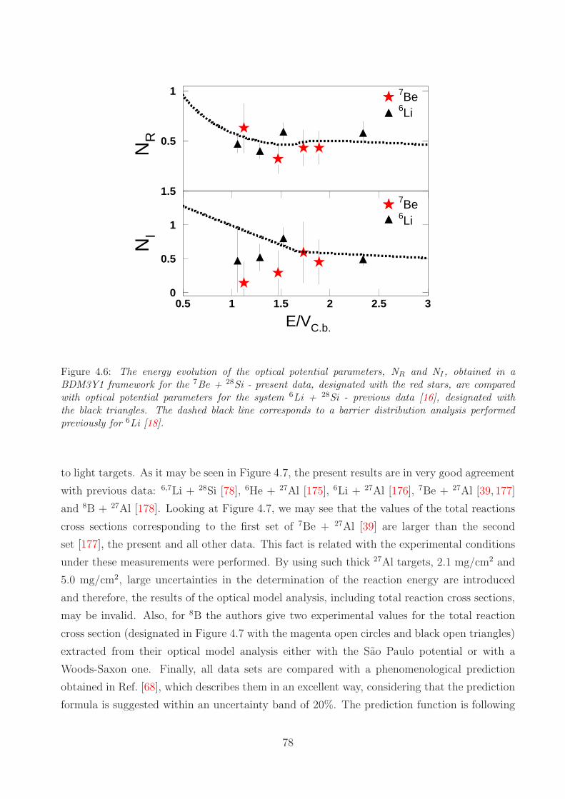
NR

7Be6Li

NI

E/VC.b.

7Be6Li

0.5

1

0.5 1 1.5 2 2.5 3

0

0.5

1

1.5

0.5 1 1.5 2 2.5 3

Figure 4.6: The energy evolution of the optical potential parameters, NR and NI , obtained in aBDM3Y1 framework for the 7Be + 28Si - present data, designated with the red stars, are comparedwith optical potential parameters for the system 6Li + 28Si - previous data [16], designated withthe black triangles. The dashed black line corresponds to a barrier distribution analysis performedpreviously for 6Li [18].

to light targets. As it may be seen in Figure 4.7, the present results are in very good agreement

with previous data: 6,7Li + 28Si [78], 6He + 27Al [175], 6Li + 27Al [176], 7Be + 27Al [39, 177]

and 8B + 27Al [178]. Looking at Figure 4.7, we may see that the values of the total reactions

cross sections corresponding to the first set of 7Be + 27Al [39] are larger than the second

set [177], the present and all other data. This fact is related with the experimental conditions

under these measurements were performed. By using such thick 27Al targets, 2.1 mg/cm2 and

5.0 mg/cm2, large uncertainties in the determination of the reaction energy are introduced

and therefore, the results of the optical model analysis, including total reaction cross sections,

may be invalid. Also, for 8B the authors give two experimental values for the total reaction

cross section (designated in Figure 4.7 with the magenta open circles and black open triangles)

extracted from their optical model analysis either with the Sao Paulo potential or with a

Woods-Saxon one. Finally, all data sets are compared with a phenomenological prediction

obtained in Ref. [68], which describes them in an excellent way, considering that the prediction

formula is suggested within an uncertainty band of 20%. The prediction function is following

78

Table 4.2: Total reaction cross sections for 7Be + 28Si obtained in the present work via anoptical model analysis, σopt, are compared with values deduced in the α-production analysis [160](see Section 4.2), σα−production, as well as with a phenomenological prediction [68], σpred anda theoretical value extracted from our CDCC calculations, σCDCC (see Subsection 4.1.4). Thefirst column includes projectile energies incident in front of the target, Elab, while the secondcolumn, the reaction energy, Erea, in the middle of the target.

Elab (MeV) Erea (MeV) σopt (mb) σα−production (mb) σpred (mb) σCDCC (mb)22.0 21.7 1124 ± 148 1206 ± 195 1118 113019.8 19.5 1072 ± 163 1103 ± 242 990 102017.2 16.7 738 ± 190 - 779 83113.2 12.9 355 ± 95 250 ± 63 347 401

Table 4.3: The barrier parameters namely, barrier height VB, radius RB and curvature ~ω,for various systems considered in this work, obtained using the Christensen-Winther potential[174].

System VB (MeV) RB (fm) ~ω (MeV)7Be + 28Si 9.351 7.922 3.4786Li + 28Si 7.008 7.932 3.2237Li + 28Si 6.840 8.145 2.9688B + 28Si 11.670 7.935 3.6627Be + 27Al 8.681 7.925 3.3719Be + 27Al 8.358 8.269 2.9556Li + 27Al 6.512 7.927 3.1236He + 27Al 4.201 8.222 2.4878B + 27Al 10.825 7.943 3.553

the equation: Y(x)= αln[1+exp(2πx-b)], with α= 1.14409 and b= -1.06089.

79

FT

R(x

)

x

Prediction

6Li+28Si7Li+28Si

6He+27Al

6Li+27Al

7Be+27Al7Be+27Al

8B+27Al

7Be+28Si - Present

1

10

10 2

-5 -2.5 0 2.5 5 7.5 10

Figure 4.7: Reduced total reaction cross sections for weakly bound projectiles on light targets. Previousdata from Refs. [39, 78, 175–178] are compared with the present data and a prediction from Ref. [68]for light targets, designated with the black solid line.

4.1.4 Continuum Discretized Coupled Channels Calculations

For a more global description of the elastic scattering of 7Be + 28Si, Continuum Discretized

Coupled Channels (CDCC) calculations were performed, taking into account couplings to

continuum states, both resonant and non-resonant ones. These calculations were performed

via the code FRESCO [98]. The model used in the calculations was very close to that of

Ref. [179]. The 7Be nucleus was modeled as a composite system with a two-body 4He + 3He

cluster structure. Couplings between resonant and non-resonant cluster states corresponding to4He - 3He relative orbital angular momentum L = 0, 1, 2, 3, 4 were included. The excitation to

first excited state of the projectile (0.429 MeV) and ground state reorientation was also taken

into account. The continuum phase space above the 7Be → 4He + 3He breakup threshold

(1.586 MeV) was discretized into momentum bins. As highest excitation energy was taken the

80

Table 4.4: Optical model parameters for the 4He + 28Si [180] and 3He + 28Si [181] interactionsadopted in the CDCC calculations. The real and imaginary parts of the optical potential aredescribed by Woods-Saxon form factors. The nuclear radius is given as R= rV (W ) * 281/3. TheCoulomb radius for the 4He(3He) + 28Si interaction was taken as RC= 1.62(1.30) * 281/3.

System V (MeV) rV (fm) aV (fm) W (MeV) rW (fm) aW (fm)4He + 28Si 82.00 1.62 0.52 13.50 1.62 0.523He + 28Si 106.50 1.07 0.85 11.80 1.80 0.65

energy of 9.4 MeV for the 22.0 and 19.8 MeV data and 7.7 MeV for the 17.2 and 13.2 MeV data.

The convergence of the calculation was tested taking into account higher excitation energies

and relative angular momenta which however did not affect the results of the calculation. The

width of the bins at the energy of 13.2 and 17.2 MeV was ∆k= 0.23 fm−1, while the width of

the bins at the energy of 19.8 and 22.0 MeV was ∆k= 0.20 fm−1. In the presence of resonant

states, the binning schemes were suitably modified in order to avoid double counting. In our

calculations, the 7/2− (4.57 MeV) and 5/2−(6.73 MeV) resonances were taken into account

and they were treated as momentum bins with a width corresponding to 0.4 and 2.0 MeV

respectively. All the diagonal and coupling potentials were generated from empirical 4He +

Target, 3He + Target optical model potentials for the corresponding target nucleus by means of

the single-folding technique. The corresponding potentials were adopted from Refs. [180, 181]

and are shown in Table 4.4.

Into this context, elastic scattering angular distributions were deduced and are compared

with the data in Figures 4.8, 4.9, 4.10 and 4.11. Furthermore, one (7Be ground state reorien-

tation only)- and two (7Be ground state reorientation and excitation of the first excited state)-

channel calculations were performed and the results are compared with the data in Figures

4.12 and 4.13. The agreement of the data with the full CDCC calculations is very good, while

it is seen that the coupling to inelastic excitations of 7Be is unimportant and couplings to

continuum are substantial but not very strong. Furthemore, our CDCC calculations provided

breakup angular distributions (Subsection 4.2.2) and total breakup cross sections. The last

are included in Table 4.5.

81

OMP fit - σ=1124 mb

CDCC - σ=1130 mb

Present data

σ/σ R

uth

θc.m.(deg)

10-2

10-1

1

0 20 40 60 80

Figure 4.8: Present angular distribution data for the elastic scattering of 7Be + 28Si at the energyof 22.0 MeV

(E/VC.b.= 1.90

), designated with the red stars, are compared with a CDCC calculation

which is denoted solid blue line. The dashed red line represents our best fit optical model calculation.

OMP fit - σ=1072 mb

CDCC - σ=1020 mb

Present data

σ/σ R

uth

θc.m.(deg)

10-2

10-1

1

0 20 40 60 80

Figure 4.9: Same as in Figure 4.8 but for the energy of 19.8 MeV(E/VC.b.= 1.71

).

82

OMP fit - σ=738 mb

CDCC - σ=831 mb

Present data

σ/σ R

uth

θc.m.(deg)

10-1

1

0 20 40 60 80

Figure 4.10: Same as in Figure 4.8 but for the energy of 17.2 MeV(E/VC.b.= 1.48

).

OMP fit - σ=355 mb

CDCC - σ=401 mb

Present data

σ/σ R

uth

θc.m.(deg)

10-1

1

0 20 40 60 80

Figure 4.11: Same as in Figure 4.8 but for the energy of 13.2 MeV(E/VC.b.= 1.14

).

83

Table 4.5: Breakup cross sections for the 7Be + 28Si system, as they were deduced from ourCDCC calculations.

Energy (MeV) Breakup (mb)22.0 13.419.8 10.517.2 7.413.2 3.4

Full CDCC

1 - channel2 - channels

Full CDCC

1 - channel2 - channels

σ/σ R

uth

θc.m.(deg)

10-2

10-1

1

0 20 40 60 80

10-1

1

0 20 40 60 80

Figure 4.12: Elastic scattering data for 7Be + 28Si at 22.0 MeV (top) and 19.8 MeV (bottom) arecompared with 1 - channel, 2 - channel and full CDCC calculations.

84

Full CDCC

1 - channel2 - channels

Full CDCC

1 - channel2 - channels

σ/σ R

uth

θc.m.(deg)

10-1

1

0 20 40 60 80

10-1

1

0 20 40 60 80

Figure 4.13: Elastic scattering data for 7Be + 28Si at 17.2 MeV (top) and 13.2 MeV (bottom) arecompared with 1 - channel, 2 - channel and full CDCC calculations.

4.2 Reaction Mechanisms

4.2.1 Fusion Cross Sections

As it was mentioned in Chapter 3, the α-particle production angular distributions are for-

ward peaked but they also extend to more backward angles with substantial cross sections.

This fact indicates the presence of both direct and compound nucleus formation mechanisms.

In order to disentangle the compound nucleus processes from the direct ones, we follow the

same technique as applied previously for the 6,7Li + 28Si systems [54, 60, 78]. The angular

distributions from evaporated α-particles were calculated within the statistical model frame-

work [182] via code PACE2(Projection Angular-momentum Coupled Evaporation

)[132]. In

the code, optical potential parameters for the evaporation of α-particles were introduced from

the work of Huizenga and Igo [183] based on α-particle scattering from very low energies up

to 50 MeV, and 20 target nuclei with 10 6 Z 6 92. The level density parameter was taken

as A/8 MeV−1, and compound nucleus spin distributions were calculated taking into account

the Bass nuclear potential [184].

The calculated angular distributions were renormalized to the data of the backward de-

85

tectors, T3 and T4. The procedure is illustrated in Figure 4.14 for 22.0, 19.8 and 13.2 MeV.

In the latter case, due to low statistics, data for the middle and backward detectors were

summed over the whole detector and the obtained differential cross sections were assigned to

the middle angle of each detector. The renormalized compound nucleus angular distributions

were integrated over angle and the α-particle production due to compound nucleus formation,

σαcompound, was obtained. The values are included in Table 4.7. The errors were assigned taking

into account the best fits and a reduced χ2-plus-1 analysis[(χ2/N) + 1

]. The statistical model

code PACE2, provides also the multiplicities for the evaporated α-particles. Therefore, it was

possible to deduce fusion cross section at three near barrier energies. However, it should be

noted that the determination of fusion cross sections may be liable to possible shortcomings of

the statistical model code. A comprehensive analysis of 8B fusion data in various compound

nucleus models [185], has pointed out this issue. Our case is slightly different, since the pa-

rameter introduced in the evaporation code, that is the total fusion cross section, does not

affect the extracted values of fusion cross sections as the calculated angular distributions are

renormalized to the backward angle experimental data. However, the α-particle multiplicities

are sensitive on the choice of the level density parameter and the optical potential parameters

for the evaporation of α’s. This may introduce uncertainties in the determination of fusion

cross sections.

In this direction, test adopting different level densities or different optical potential param-

eters were carried out. By varying the level densities approximately ± 6% (A/7.5 or A/8.5),

the calculated multiplicities are larger or smaller 1% to 2%, introducing a negligible error to

the fusion. Thus, we have estimated the error introduced in the multiplicities by using three

different sets of optical model parameters from the work of Huizenga and Igo [183], McFadden

and Satchler [186] and Satchler [187]. The last two are based on the analysis of 24.7 and

28.0 MeV α-particle scattering on various targets with atomic numbers, 8 6 Z 6 92 and 10

6 Z 6 50 respectively. The calculated multiplicities together with the mean and a standard

deviation are presented in Table 4.6. Subsequently, using the α-particle multiplicities and the

cross sections due to compound nucleus formation, fusion cross sections were deduced. The

values are included in Table 4.7 and they are also compared with a single barrier penetration

model (BPM) prediction of Wong [74].

The fusion cross sections, presented in Table 4.7, were considered in a systematics involving

other, stable, weakly bound and radioactive projectiles on the same or similar mass targets

(27Al, 28Si). However, in order to compare fusion cross sections corresponding to various

systems, the different data sets should be reduced appropriately such as to exclude static

86

a)PACE2Data

(dσ/

dΩ) la

b(m

b/sr

)

b)PACE2Data

θlab(deg)

c)PACE2

Data

10

10 2

0 20 40 60 80 100 120 140

10

10 2

0 20 40 60 80 100 120 140

1

10

10 2

0 20 40 60 80 100 120 140

Figure 4.14: Present angular distribution data for the 4He particle production at the energies of a) 22.0MeV, b) 19.8 MeV and c) 13.2 MeV. The solid blue line represents a calculation with the evaporationcode PACE2 renormalized to the backward angle data. For the energy of 13.2 MeV, the black squarerepresents the experimental datum minus the estimated contribution from direct processes, since inthat case we expect significant direct contribution.

87

Table 4.6: α-particle multiplicities obtained via statistical code PACE2 [132] using three dif-ferent sets of optical potentials. The second column includes multiplicities using the Huizengaand Igo potential [183], M1, the third column using the McFadden and Satchler potential [186],M2, the fourth column using the Satchler potential [187], M3, while the last column includesthe mean of these multiplicities, Mmean, and the standard deviation.

Energy (MeV) M1 M2 M3 Mmean

22.0 0.63 0.55 0.58 0.59 ± 0.0419.8 0.57 0.50 0.52 0.53 ± 0.0413.2 0.37 0.31 0.34 0.34 ± 0.03

effects for each system arising from the different barrier heights, radii and curvatures. The

reduction procedure adopted in this work follows the prescription described in Refs. [169–172],

based on a single barrier penetration model of Wong. Wong has approximated the barriers

for different partial waves, ℓ, by inverted harmonic oscillator potentials of height VBℓ and

frequency ωℓ. By using the assumption that the radii and curvatures of the potentials do not

vary with angular momentum, Wong obtained for fusion the following analytic expression:

σWongfusion =

~ωR2B

2Ec.m.∗ ln

[

1 + exp

(

2π(Ec.m. − VB)

~ω

)]

. (4.3)

Into this context, fusion cross sections can be reduced to fusion functions, F(x), as a

function of quantity x, according to the following relations:

σfusion → F (x) =2Ec.m.

~ωR2B

∗ σfusion (4.4)

and

Ec.m. → x =Ec.m. − VB

~ω. (4.5)

88

Table 4.7: Details of our results for the compound nucleus channel. The second column in-cludes the cross section for the α-particle production due to compound nucleus formation. Thethird column includes the α-particle multiplicities obtained via the statistical code PACE2. Thefourth column includes the extracted fusion cross sections, σfusion, and the last column a pre-diction for fusion cross section according to a single barrier penetration model of Wong [74].

Energy (MeV) σαcompound (mb) α multiplicity σfusion (mb) σWong

fusion (mb)

22.0 511 ± 87 0.59 ± 0.04 866 ± 159 91019.8 419 ± 105 0.53 ± 0.04 791 ± 205 79113.2 50 ± 18 0.34 ± 0.03 147 ± 54 202

F(x

)

x

UFF6Li+28Si7Li+28Si9Be+27Al

6Li+28Si7Li+28Si7Be+27Al

8B+28Si

7Be+28Si-Present

10-1

1

10

-2 0 2 4 6

Figure 4.15: Reduced fusion cross sections for various stable and weakly bound (stable or radioactive)projectiles incident on 27Al and 28Si targets as a function of parameter x (reduced energy). Thereduction was made according to Refs. [169–172]. The solid black line represents the Universal FusionFunction, UFF, defined in [171]. Previous data were taken from Refs. [78,83,177,188–192].

89

R

x

F(x)6Li / F(x)7Li + 28Si

F(x)6Li / F(x)7Li + 59Co

F(x)6Li / F(x)7Li + 24Mg

F(x)6Li / F(x)7Li + 28Si

F(x)6Li / F(x)7Li + 64Zn

F(x)6Li / F(x)7Be + 28Si

0

0.5

1

1.5

2

2.5

3

3.5

4

-1 0 1 2 3

Figure 4.16: Ratios of fusion functions for 6Li + 28Si versus 7Li + 28Si compared with ratios of fusionfunctions for 6Li + 28Si versus 7Be + 28Si as a function of parameter x (reduced energy). Other ratiosfor 6Li versus 7Li on various low and medium mass targets are also included.

Fusion functions, F(x), were determined for various systems and they are compared among

themselves in Figure 4.15. The potential barrier parameters namely, barrier heights VB, radii

RB and curvatures ~ω for the different systems were obtained using the Christensen-Winther

potential [174] and are included in Table 4.3. Looking in Figure 4.15, present and previous

data follow the same trend as the Universal Fusion Function (UFF), defined in Ref. [171] as:

F0(x) = ln[

1 + exp(2πx

)]

, (4.6)

and show good consistency between each other as well as the UFF to within an uncer-

tainty band of 10% to 20%. Variations between the data and the UFF are expected since the

experimental values for fusion, are given, in principle, at least with an error ∼ 10%. Also,

Wong’s approximation does not take into account couplings to direct mechanisms like breakup

or transfer which are expected to be important around and below barrier. However, to assign

90

such variations with significance to a particular coupling scheme, the uncertainties to fusion

cross sections should be small, which is not in the present case. Nevertheless, we may try to

map variations between fusion cross sections obtained for 6Li and 7Li with those for 7Be, in

order to strengthen (or not) our results obtained from the optical model analysis that point to

a similarity between the two mirror nuclei, 7Li and 7Be. In this direction, ratios of fusion func-

tions for 6Li to those for 7Li and 7Be were formed. Comparisons of previously measured data

for 6,7Li + 24Mg [82], 6,7Li + 28Si [78], 6,7Li + 28Si [83], 6,7Li + 59Co [80] and 6,7Li + 64Zn [81]

with present results are shown in Figure 4.16. It is seen that hindrance of fusion cross sections

for 7Li with respect to those of 6Li, starts near barrier (already at ∼ E= 1.1VC.b., R= 1.5) and

it reaches the order of ∼ 70% well below barrier. The same trend is met for the present data

indicating a similarity between 7Be and 7Li rather than 6Li as theory had predicted for elastic

scattering in Ref. [179]. However, it should be noted that in Ref. [179], CDCC calculations

were performed for the elastic scattering of 6,7Li and 7Be on the heavy 208Pb target, where

couplings to breakup could play an important role.

4.2.2 Direct Reactions Cross Sections

In the previous Section, cross sections due to compound nucleus formation were determined

by renormalizing the theoretical compound nucleus angular distributions to the backward angle

data of the experimental (total) α-particle angular distributions. By subtracting from the ex-

perimental (total) cross sections the renormalized compound values at each angle, the angular

distributions due to direct mechanisms were obtained. As it was already mentioned in Chap-

ter 3, different direct processes contribute to the α-particle cross section. Theoretical angular

distributions for the n-pickup and n-stripping processes were obtained in the DWBA frame-

work, while for the breakup the α angular distributions were obtained in a CDCC framework.

The relevant transformations of the theoretical angular distributions from the center-of-mass

frame to the laboratory one were performed using the same Monte Carlo code used in the

spectrum simulations. The so obtained angular distributions are compared with the data in

Figure 4.17. Looking at Figure 4.17, it can be seen that the α-particle production due to these

processes is small. The remaining part should be therefore attributed to an 3He stripping pro-

cess, but which cannot be quantified by DWBA calculations due to the lack of the appropriate

spectroscopic factors (see Subsection 4.2.3).

For the 3He-particle production, the only two contributing mechanisms are the 4He strip-

ping and the breakup. However, due to the low statistics and the geometrical efficiency of our

detector setup, coincidence events between 3He and 4He particles, a clear signature of an ex-

91

clusive breakup event, were not recorded. Therefore, integrating the 3He angular distributions,

we can provide an inclusive cross section for both reaction channels. The results are given in

Table 4.8. Moreover, theoretical angular distributions for the 4He stripping and breakup were

obtained in the DWBA and CDCC frameworks respectively and are compared to the exper-

imental data in Figure 4.18. The “total” angular distributions, obtained as the sum of the

angular distributions for the breakup and 4He stripping, are in reasonable qualitative agree-

ment with the experimental data, while underestimate them in absolute magnitudes. This may

be explained from the fact that absolute spectroscopic factors for α transfer, introduced in the

DWBA calculation for the 28Si(7Be,3He)32S reaction, are notoriously ill defined. The values of

the spectroscopic factors extracted from experiments with the same target but using different

reactions and at different energies, may vary by a factor of 5 or more. Therefore, taking into

account that according to CDCC calculations, which described in a very good way the elastic

scattering data, the contribution of the breakup channel is small, we can say that the bulk

of the 3He production is attributed to 4He stripping. This is consistent with previous data

concerning the 7Be+58Ni system [67] and it seems to be a more general property of reactions

involving weakly bound nuclei presenting a cluster structure. For example, in Ref. [57], where

exclusive measurements are reported for 7Li+93Nb, t stripping is suggested as the main direct

mechanism for the α production.

Finally, having obtained cross sections for the 3,4He production due to direct mechanisms

and fusion cross sections, total reaction cross sections were deduced by summing these two

components. To avoid double summing the breakup channel, present in both 3He and 4He-

particle production, we have subtracted the breakup cross section estimated via the CDCC

calculations. Also, to avoid double counting of α’s from the decay of 8Be (n-pickup reaction)

which breaks into two α particles, we have subtracted the cross section estimated via the

DWBA calculations. Both these contributions are very small and do not significantly affect

the final result. The values of the total reaction cross sections, extracted from the α produc-

tion measurement, are given in the sixth column of Table 4.8. Also, a comparison between

these values and the ones obtained from the present optical model analysis, from our CDCC

calculations and a prediction formula described in Ref. [68] is presented in Table 4.9. All val-

ues are in very good agreement with each other indicating the validity of the measurements.

Subsequently, ratios of the direct versus total reaction cross sections were formed. The present

ratios are compared with previous ones for the systems 6,7Li + 28Si [68, 78] in Figure 4.19.

The trend of the energy evolution of the ratio for the three projectiles is the same, that is

approaching the barrier from higher to lower energies, the contribution of the direct channels

becomes larger. However, the present data seem to follow in magnitude those of 7Li rather

92

Table 4.8: 4He and 3He- particle production cross sections. The second column includes thecross section for 4He-particle production. The third and fourth columns include the 4He- and3He- particle production cross sections, respectively, due to direct mechanisms. The fifth columnincludes total cross sections due to the direct channels, deduced as the sum of 4He and 3Hecross sections after subtracting a small part due to breakup and due to double α-productionin the 8Be + 27Si channel. The breakup cross sections were estimated in a CDCC approachresulting 13.4 mb, 10.5 mb and 3.4 mb for 22.0 MeV, 19.8 MeV and 13.2 MeV respectively.The transfer pickup was estimated in a DWBA calculation and the parts subtracted were 12.5mb, 12.0 mb and 5.0 mb for 22.0 MeV, 19.8 MeV and 13.2 MeV respectively. Finally, thesixth column includes total reaction cross sections by summing fusion cross sections and directcross sections (the fifth column of this table and the fourth column of Table 4.7).

Energy (MeV) σαtotal (mb) σα

direct (mb) σ3Hedirect (mb) σdirect (mb) σα−production (mb)

22.0 763 ± 69 252 ± 111 114 ± 17 340 ± 112 1206 ± 19519.8 653 ± 72 234 ± 127 101 ± 19 312 ± 128 1103 ± 24213.2 131 ± 26 81 ± 32 30 ± 8 103 ± 33 250 ± 63

Table 4.9: Total reaction cross sections for 7Be + 28Si extracted from the α-production analysis,σα−production, are compared with values deduced in the present optical model analysis, σopt,as well as with the theoretical values extracted from our CDCC calculations, σCDCC and aphenomenological prediction [68], σpred. The first column includes projectile energies incidentin front of the target and the second column breakup cross sections, σbu, deduced from ourCDCC calculations.

Elab (MeV) σbu (mb) σα−production (mb) σopt (mb) σCDCC (mb) σpred (mb)22.0 13.4 1206 ± 195 1124 ± 148 1130 111819.8 10.5 1103 ± 242 1072 ± 163 1020 99017.2 7.4 - 738 ± 190 831 77913.2 3.4 250 ± 63 355 ± 95 401 347

than those for 6Li. This indicates larger contribution of direct processes for the two mirror

nuclei than for 6Li. Approaching the barrier from higher to lower energies, direct channels

exhaust the largest part of the total reaction cross section (70% of the total reaction cross

section) and this may be the reason for fusion hindrance, observed for 7Li and 7Be compared

to 6Li (Figure 4.16). It should be underlined that more data for the 7Be below barrier are

needed, in order to draw firm conclusions.

4.2.3 DWBA Calculations

The direct reactions (except the breakup one) leading to 3He and 4He- particle production

were described in the DWBA framework [123]. In all cases, the potential of the entrance

93

channel (7Be + 28Si) was described using the global 7Li optical model parameters of Cook

[193]. For the rest of the details, we will refer to each reaction seperately starting with the28Si(7Be,6Be)29Si reaction.

Considering the unbound nature of 6Be, there are no optical model parameters available for

reactions involving this nucleus. Instead, the global 6Li optical model parameters of Cook [193]

were used. Stripping to both the 0+ ground state and 1.67 MeV 2+ resonances of 6Be was

included. The spectroscopic factors for the⟨7Be | 6Be + n

⟩overlaps were taken from Ref. [194].

The valence neutron was bound to a 6Be core in a Woods-Saxon well of radius 1.25 × A1/3 fm

and diffuseness 0.65 fm. A Thomas-form spin-orbit potential of the same geometry and fixed

depth of 6.0 MeV was also included, while the depth of the central well was adjusted such as

to reproduce the experimental binding energy. Moreover, stripping to the following states of29Si was included: 0.0 MeV 1/2+, 1.27 MeV 3/2+, 2.03 MeV 5/2+, 3.62 MeV 7/2−, 4.94 MeV

3/2− and 6.20 MeV 7/2−. The spectroscopic factors for the⟨29Si | 28Si + n

⟩overlaps were

taken from Ref. [195].

For the 28Si(7Be,8Be)27Si reaction, since 8Be is also unbound, the global 7Li optical model

parameters from Ref. [193] were used for the exit channel potential. Pickup to both the 0+

ground state and 3.03 MeV 2+ resonances of 8Be was included and the spectroscopic factors

for the⟨8Be | 7Be + n

⟩overlaps were taken from Ref. [194]. The valence neutron was bound to

a 7Be core in a Woods-Saxon well of radius 1.25 × A1/3 fm and diffuseness 0.65 fm. A Thomas-

form spin-orbit potential of the same geometry and fixed depth of 6.0 MeV was also included,

while the the depth of the central well was adjusted such as to reproduce the experimental

binding energy. Moreover, pickup leading to the following states of 27Si was included: 0.0 MeV

5/2+, 0.78 1/2+ and 0.96 MeV 3/2+. The spectroscopic factors for the⟨28Si | 27Si + n

⟩overlaps

were taken from Ref. [196]. In this reaction, the 8Be ejectile decays to two α particles. This

was taken into account in producing the angular distributions illustrated in Figure 4.17.

The calculations for the 28Si(7Be,4He)31S reaction are more erratic, since there are no suit-

able spectroscopic factors available in the literature for the⟨31S | 28Si + 3He

⟩overlaps. The

only experimental indication for population of states in 31S comes from a measurement of

the 28Si(6Li,3H)31S reaction [197]. Here the 0.0 MeV 1/2+, 1.25 MeV 3/2+, and 4.45 MeV

7/2− states were the main states observed in 31S. The Q-matching conditions for this reac-

tion favor the population of highly exited states (Eexc > 10 MeV) close to or above the 3He

emission threshold. Therefore, such calculations were not performed since there is insufficient

information available to yield meaningful results.

Finally, in case of the 28Si(7Be,3He)32S reaction the global 3He optical model parameters

94

of Ref. [198] were used for the exit channel potential. The spectroscopic factor for the⟨7Be |

4He + 3He⟩overlap was set equal to 1.0 and the 4He + 3He binding potential was taken from

Ref. [199]. Stripping leading to the following states in 32S was included: 0.0 MeV 0+, 2.23

MeV 2+, 3.78 MeV 0+, 4.46 MeV 4+, 5.01 MeV 3−, 5.80 MeV 1−, 6.76 MeV 3−, 7.43 MeV

1−, and 8.49 MeV 1−. Since the last two states are unbound with respect to the 4He emission

threshold of 32S, the form factors in this particular case were calculated using the weak binding

energy approximation with a “binding energy” of 0.01 MeV. For these states, spectroscopic

factors were considered from the reaction 28Si(6Li,d)32S reported in Ref. [200].

95

a)

Breakup (x2)Total (x2)

n-stripping (x2)n-pickup (x2)

Data

(dσ/

dΩ) la

b(m

b/sr

)

b)

Breakup (x2)Total (x2)

n-stripping (x2)n-pickup (x2)

Data

θlab(deg)

c)

Breakup (x4)Total (x2)

n-stripping (x12)n-pickup (x2)

Data

1

10

10 2

0 20 40 60 80 100 120

1

10

10 2

0 20 40 60 80 100 120

1

10

10 2

0 20 40 60 80 100 120

Figure 4.17: Angular distributions for α-particle production due to direct processes at (a) 22.0 MeV,(b) 19.8 MeV and (c) 13.2 MeV. Experimental data are denoted with the black open circles, DWBAcalculations for neutron stripping with the dashed green line and for neutron pickup with the dottedcyan line, while CDCC calculations for the breakup are denoted with the dotted-dashed blue line. Thesum of the three processes is depicted with the solid red line. The remaining part may be attributed to3He stripping. The multiplication factors are arbitrary for a better display of the various processes.Errors in the data are solely due to the experimental uncertainties of total α production.

96

Dataa)Breakup

4He stripping

Total

(dσ/

dΩ) la

b(m

b/sr

)

Datab)Breakup

4He stripping

Total

θlab(deg)

Datac)Breakup (x4)

4He stripping

Total

1

10

10 2

0 10 20 30 40 50 60 70 80 90

1

10

10 2

0 10 20 30 40 50 60 70 80 90

1

10

10 2

0 10 20 30 40 50 60 70 80 90

Figure 4.18: Angular distributions for 3He-particle production at (a) 22.0 MeV, (b) 19.8 MeV and(c) 13.2 MeV. Experimental data are denoted with the red circles, DWBA calculations for the 4Hestripping with the dashed green line and CDCC calculations for the breakup are denoted with thedotted-dashed blue line. The sum of the two processes is depicted with the solid black line. Themultiplication factor (panel c) for breakup is arbitrary, for a better visual view.

97

R

E/VC.b.

Prediction

CDCC-7Li+28Si

CDCC-6Li+28Si

7Be+28Si-Present7Li+28Si6Li+28Si

DWBA*5-7Be+28Si-Present

0

0.2

0.4

0.6

0.8

1

0.5 1 1.5 2 2.5

Figure 4.19: Energy evolution of ratios, R, of direct to total reaction cross sections. The present resultsfor 7Be + 28Si, designated with the solid blue circles, are compared with previous results for 6Li +28Si(red stars) and 7Li + 28Si(green square) [17]. They are also compared with a phenomenologicalprediction(solid blue line) for 7Be + 28Si, outlined in Ref. [68]. Previous calculated ratios for 6Li +28Si and 7Li + 28Si are also shown as the dotted-dashed red line and dotted green line, respectively [78].These calculations were based on total reaction cross sections deduced from a CDCC calculation andfusion cross sections deduced from a BPM model. In the latter case an energy dependent potential wastaken into account, derived from the CDCC calculations according to the prescription of Thompson[201]. The open circles correspond to the present DWBA calculations, multiplied by 5 to match thedata.

98

Chapter 5

Conclusions - Summary

In the present work, we have investigated the elastic scattering and the relevant reaction

mechanisms for the system 7Be + 28Si at near barrier energies. Angular distribution for the

elastically scattered 7Be ions were obtained at four energies, namely 22.0, 19.8, 17.2 and 13.2

MeV(E/VC.b.= 1.14, 1.48, 1.71, 1.90

), while angular distribution for the reaction products

3He and 4He, the cluster constituents of 7Be, were obtained at 22.0, 19.8 and 13.2 MeV.

The elastic scattering data were analyzed into a double folding framework by using the

BDM3Y1 interaction and the energy evolution of the real and imaginary part of the optical

potential was deduced. Due to the large errors, it was not possible to draw firm conclusions

solely from the elastic scattering data but only in conjunction with the α - production ones.

However, from the elastic scattering data, the trend seems to be compatible with a standard

threshold anomaly at least in what concerns the imaginary part, with a decreasing magnitude

as we approach the barrier from higher to lower energies. The agreement of the present

data with a dispersion relation cannot be confirmed, as in the critical position of the real

potential, where a peak should appear, we possess only one datum. On the other hand, taking

into account all information relevant to previous data of 6,7Li + 28Si, analyzed in the same

framework as is the present case, we can in principle conclude that both mirror nuclei, 7Li

and 7Be present the same energy dependence of the optical potential. This is close to the

standard threshold anomaly, from the point of view of the decreasing imaginary potential but

where possibly the dispersion relation does not hold [19]. This evidence, if combined with the

results of the α - production data, collected at the same experiment and reported in Ref. [160],

indicates with some confidence the similarity between the two mirror nuclei. In Ref. [160], the

fusion hindrance of both 7Li and 7Be versus 6Li was reported and the similarity between the

two mirror nuclei was suggested. Based on the fact that two different reaction channels yielded

99

the same result, we can confirm in this study the similarity between the two mirror nuclei, 7Li

and 7Be.

Our optical model analysis also yielded total reaction cross sections which were found to

be in very good agreement with the values obtained via the present analysis of 3,4He-particle

production and global phenomenological predictions [68]. As total reaction cross sections are

traditionally used to restrict the imaginary part of the optical potential, this compatibility

further supports our result for the energy dependence of the optical potential. This raises

questions for the dependence of the new or the standard threshold anomaly on the breakup

threshold. 7Be nucleus has a breakup threshold of 1.59 MeV similar to that of 6Li, 1.47 MeV,

and not of 7Li with 2.47 MeV, but still it resembles rather its mirror encounter and not 6Li.

Further on, our total reaction cross sections were also considered in a systematic framework

and were found in very good compatibility with results of other weakly bound, stable as well

as radioactive, projectiles on similar mass targets.

For a more global description of the elastic scattering data, we have performed one, two

channel and full CDCC calculations. It was found that the coupling to inelastic excitations of7Be is unimportant, while couplings to continuum are substantial but not very strong.

From the point of view of reaction mechanisms, according to the measured light-particle

production and the calculations of relevant compound-nucleus and direct single neutron strip-

ping and pickup reaction processes, large 3He- and 4He-stripping channels may be inferred.

These were obtained by subtracting from total direct cross sections the single neutron strip-

ping and pickup channel contribution. It should be noted that the DWBA calculations [123] of

single neutron stripping and pickup should be reasonably quantitatively accurate, since such

processes are usually well described. Also, the contribution of the breakup to the 3,4He-particle

production is estimated to be small according to our CDCC calculations. Therefore, strong3He-4He reaction channels are inferred.

The relevant DWBA calculations for the 28Si(7Be,4He)31S and 28Si(7Be,3He)32S reactions

which might shed more light on the large 3He- and 4He- particle production are erratic. The

optimum Q-values vary from -4 to -8 MeV and -4 to ∼-9 for the first and the second reaction

respectively, for incident energies of 13.2 to 22.0 MeV. This implies preferential population

of states in the residual nucleus at excitation energies where no spectroscopic factors are

available. Thus, theoretical calculations for the 28Si(7Be,4He)31S were not performed. In

case of the 28Si(7Be,3He)32S reaction, DWBA calculations were performed, using the available

spectroscopic factors which however correspond to a limited excitation energy range in the 32S

covered by the Q optimum value. It was found that the calculations underpredict the data.

100

This may be due to the fact that absolute spectroscopic factors for α transfer reactions are

ambiguously determined and in fact, factors of 5 or more between values for the same target

obtained with different reactions and at different bombarding energies are common. This may

easily explain why, although the DWBA calculations are in reasonable qualitative agreement

with the data, underpredict their absolute values.

The compound nucleus contribution to the total α-particle production was estimated by

renormalizing the theoretical angular distributions from evaporated α-particles, calculated

within the statistical model framework [182], to the backward angle data, enabling the direct

component to be separated. Subsequently, using the α-particle multiplicities, calculated in the

same statistical framework, and the cross sections due to compound nucleus formation, fusion

cross sections were deduced. Fusion cross sections were considered in a systematics involving

other, stable weakly bound and radioactive projectiles on the same or similar mass targets and

present good consistency between each other as well as the UFF to within an uncertainty band

of 10% to 20%. This does not preclude the behavior observed below the barrier for the same

projectile but heavier targets, where small to very large enhancements have been reported.

It is therefore an open question whether fusion below the barrier for proton rich nuclei is

enhanced, in contrast to the behavior of neutron rich nuclei, and whether this is connected

with the target mass. It should be underlined, however, that the present results, considered in

a systematic framework with the low mass target 28Si, indicate a hindrance of fusion below the

barrier rather than an enhancement. This hindrance was observed before for 7Li on various

targets [78, 80–83] indicating a similarity between the two mirror nuclei.

Total reaction cross sections were formed as the sum of direct and fusion cross sections and

the energy evolution of the ratio direct to total was mapped. The energy evolution for the

system under study exhibits the same increasing trend approaching the barrier from higher

to lower energies as for the stable weakly bound projectiles 6Li and 7Li on the same target.

However, the results follow in magnitude those for 7Li, where we observe larger direct to total

ratios due to an enhancement of transfer channels at the expense of fusion. Indeed, the present

fusion results for 7Be, if compared with those for 6,7Li on the same target, 28Si, are in perfect

agreement with previous results for 7Li. This fact, as it was already mentioned above, together

with the results obtained from our optical model analysis present a strong evidence that 7Be

resembles its mirror nucleus, 7Li, and not 6Li one.

In summary,

The energy dependence of the optical potential was sought for the system 7Be + 28Si at near

101

barrier energies via elastic scattering measurements. Comparisons between 7Be -present data

and 6,7Li -previous data on the same target showed that, 7Be resembles its mirror nucleus and

not 6Li one. The behavior of imaginary part of the optical potential is compatible with the

standard threshold anomaly, while the real part cannot be definitely interpreted into dispersion

relations framework, due to the limited data points around Coulomb barrier. It should be noted

that the similarity between 7Be and 7Li is also validated from the analysis of fusion data, where

fusion hindrance is indicated below barrier for both 7Be and 7Li nuclei. This may be related

to the large transfer cross sections, observed for the two mirror nuclei, which act at expense

of the fusion ones. In our case, the bulk of the transfer cross sections is attributed to 3He and4He stripping reactions.

102

References

[1] J. S. Lilley, B. R. Fulton, M. A. Nagarajan et al., Phys. Lett. B 151, 181 (1985).

[2] A. Baeza, B. Bilwes, R. Bilwes et al., Nucl. Phys. A 419, 412 (1984).

[3] M. A. Nagarajan, C. C. Mahaux and G. R. Satchler, Phys. Rev. Lett. 54, 1136 (1985).

[4] C. Mahaux, H. Ngo, G. R. Satchler, Nucl. Phys. A 449, 354 (1986).

[5] G. R. Satchler, Phys. Rep. 199, 147 (1991).

[6] L. F. Canto, P. R. S. Gomes, R. Donangelo et al., Phys. Rep. 424, 1 (2006).

[7] N. Keeley, R. Raabe, N. Alamanos et al., Prog. Part. Nucl. Phys. 59, 579 (2007).

[8] N. Keeley, N. Alamanos, K. W. Kemper et al., Prog. Part. Nucl. Phys. 63, 396 (2009).

[9] P. R. S. Gomes, J. Lubian, L. F. Canto et al., Few-Body Syst. 57, 165 (2016).

[10] C. Beck, Nucl. Phys. A 787, 251c (2007).

[11] C. Beck, N. Rowley, P. Papka et al., Nucl. Phys. A 834, 440c (2010).

[12] Y. Sakuragi, M. Yahiro and M. Kamimura, Prog. Theor. Phys. 68, 322 (1982).

[13] Y. Sakuragi, M. Yahiro and M. Kamimura, Prog. Theor. Phys. 70, 322 (1983).

[14] N. Keeley, S. J. Bennett, N. M. Clarke et al., Nucl. Phys. A 571, 326 (1994).

[15] A. M. M. Maciel, P. R. S. Gomes, J. Lubian et al., Phys. Rev. C 59, 2103 (1999).

[16] A. Pakou, N. Alamanos, A. Lagoyannis et al., Phys. Lett. B 556, 21 (2003).

[17] A. Pakou, N. Alamanos, G. Doukelis et al., Phys. Rev. C 69, 054602 (2004).

[18] K. Zerva, N. Patronis, A. Pakou et al., Phys. Rev. C 80, 017601 (2009).

103

[19] K. Zerva, A. Pakou, K. Rusek et al., Phys. Rev. C 82, 044607 (2010).

[20] K. Zerva, A. Pakou, N. Patronis et al., Eur. Phys. Journal A 48, 102 (2012).

[21] M. S. Hussein, P. R. S. Gomes, J. Lubian et al., Phys. Rev. C 73, 044610 (2006); Erratum,

Phys. Rev. C 76, 019902(E) (2007).

[22] J. M. Figueira, D. Abriola, J. O. Fernandez Niello et al., Phys. Rev. C 73, 054603 (2006).

[23] M. Biswas, Subinit Roy, M. Sinha et al., Nucl. Phys. A 802, 67 (2008).

[24] F. A. Souza, L. A. S. leal, N. Carlin et al., Phys. Rev. C 75, 044601 (2007).

[25] M. Zadro, P. Figuera, A. Di Pietro et al., Phys. Rev. C 80, 064610 (2009).

[26] L. Fimiani, J. M. Figueira, G. V. Martı et al., Phys. Rev. C 86, 044607 (2012).

[27] H. Kumawat, V. Jha, B. J. Roy et al., Phys. Rev. C 78, 044617 (2008).

[28] N. N. Deshmukh, S. Mukherjee, D. Patel et al., Phys. Rev. C 83, 024607 (2011).

[29] J. M. Figueira, J. O. Fernandez Niello, A. Arazi et al., Phys. Rev. C 81, 024613 (2010).

[30] S. Santra, S. Kailas, K. Ramachandran et al., Phys. Rev. C 83, 034616 (2011).

[31] Shradha Dubey, S. Mukherjee, D. C. Biswas et al., Phys. Rev. C 89, 014610 (2014).

[32] L. F. Canto, P. R. S. Gomes, R. Donangelo et al., Phys. Rep. 596, 1 (2015).

[33] A. M. Sanchez-Benıtez, D. Escrig, M. A. G. Alvarez et al., Nucl. Phys. A 803, 30 (2008).

[34] L. Acosta, A. M. Sanchez-Benıtez, M. E. Gomez et al., Phys. Rev. C 84, 044604 (2011).

[35] A. R. Garcia, J. Lubian, I. Padron et al., Phys. Rev. C 76, 067603 (2007).

[36] A. Gomez Camacho, E. F. Aguilera, E. Martınez Quiroz et al., Nucl. Phys. A 833, 156

(2010).

[37] A. Gomez Camacho, E. F. Aguilera, P. R. S. Gomes et al., Phys. Rev. C 84, 034615

(2011).

[38] A. Gomez Camacho and E. F. Aguilera, Phys. Rev. C 90, 064607 (2014).

[39] V. Morcelle, R. Lichtenthaler, R. Linares et al., Phys. Rev. C 89, 044611 (2014).

104

[40] A. Di Pietro, V. Scuderi, A. M. Moro et al., Phys. Rev. C 85, 054607 (2012).

[41] M. Cubero, J. P. Fernandez-Garcıa, M. Rodrıguez-Gallardo et al., Phys. Rev. Lett. 109,

262701 (2012).

[42] J. P. Fernandez-Garcıa, M. Cubero, L. Acosta et al., Phys. Rev. C 92, 044608 (2015).

[43] K. Rusek, N. Keeley, K. W. Kemper et al., Phys. Rev. C 67, 041604(R) (2003).

[44] Y. Kucuk, I. Boztosun and N. Keeley, Phys. Rev. C 79, 067601 (2009).

[45] N. Keeley, N. Alamanos, K. Rusek et al., Phys. Rev. C 71, 014611 (2005).

[46] A. Pakou, N. Alamanos, N. M. Clarke et al., Phys. Lett. B 633, 691 (2006).

[47] F. A. Souza, C. Beck, N. Carlin et al., Nucl. Phys. A 821, 36 (2009).

[48] F. A. Souza, N. Carlin, C. Beck et al., Nucl. Phys. A 834, 420c (2010).

[49] F. A. Souza, N. Carlin, C. Beck et al., Eur. Phys. Journal A 44, 181 (2015).

[50] C. Signorini, A. Edifizi, M. Mazzocco et al., Phys. Rev. C 67, 044607 (2003).

[51] D. H. Luong, M. Dasgupta, D. J. Hinde et al., Phys. Rev. C 88, 034609 (2013).

[52] S. Santra, V. V. Parkar, K. Ramachandran et al., Phys. Lett. B 677, 139 (2009).

[53] J. J. Kolata, H. Amro, F. D. becchetti et al., Phys. Rev. C 75, 031302(R) (2007).

[54] A. Pakou, K. Rusek, N. Alamanos et al., Phys. Rev. C 76, 054601 (2007).

[55] D. Gupta, C. Samanta, R. Kanungo et al., Nucl. Phys. A 646, 161 (1999).

[56] A. Shrivastava, A. Navin, N. Keeley et al., Phys. Lett. B 633, 463 (2006).

[57] S. K. Pandit, A. Shrivastava, K. Mahata et al., Phys. Rev. C 93, 061602(R) (2016).

[58] D. Gupta, C. Samanta, A. Chatterjee et al., Nucl. Phys. A 683, 3 (2001).

[59] A. Pakou, N. Alamanos, A. Gillibert et al., Phys. Rev. Lett. 90, 202701 (2003).

[60] A. Pakou, N. G. Nicolis, K. Rusek et al., Phys. Rev. C 71, 064602 (2005).

[61] H. Kumawat, V. Jha, V. V. Parkar et al., Phys. Rev. C 81, 054601 (2010).

[62] C. S. Palshetkar, S. Santra, A. Shrivastava et al., Phys. Rev. C 89, 064610 (2014).

105

[63] V. Scuderi, A. Di Pietro, P. Figuera et al., Phys. Rev. C 84, 064604 (2011).

[64] A. Di Pietro, P. Figuera, F. Amorini et al., Phys. Rev. C 69, 044613 (2004)

[65] E. F. Aguilera, J. J. Kolata, F. M. Nunes et al., Phys. Rev. Lett. 84, 5058 (2000).

[66] D. Escrig, A. M. Sanchez-Benıtez, A. M. Moro et al., Nucl. Phys. A 792, 2 (2007).

[67] M. Mazzocco, D. Torresi, D. Pierroutsakou et al., Phys. Rev. C 92, 024615 (2015).

[68] A. Pakou, D. Pierroutsakou, M. Mazzocco et al., Eur. Phys. Journal A 51, 55 (2015).

[69] J. J. Kolata, V. Guimaraes, D. Peterson et al., Phys. Rev. Lett. 81, 4580 (1998).

[70] E. Martinez-Quiroz, E. F. Aguilera, D. Lizcano et al., Phys. Rev. C 90, 014616 (2014).

[71] R. Raabe, J. L. Sida, J. L. Charvet et al., Nature (London) 431, 823 (2004).

[72] A. Lemasson, A. Shrivastava, A. Navin et al., Phys. Rev. Lett. 103, 232701 (2009).

[73] R. Raabe, C. Angulo, J. L. Charvet et al., Phys. Rev. C 74, 044606 (2006).

[74] C. Y. Wong, Phys. Rev. Lett. 31, 766 (1973).

[75] A. Pakou and K. Rusek, Phys. Rev. C 69, 057602 (2004).

[76] A. Pakou, Phys. Rev. C 78, 067601 (2008).

[77] D. Roubos, A. Pakou, N. Alamanos et al., Phys. Rev. C 73, 051603(R) (2006).

[78] A. Pakou, K. Rusek, N. Alamanos et al., Eur. Phys. Journal A 39, 187 (2009).

[79] A. Pakou, A. Musumarra, D. Pierroutsakou et al., Nucl. Phys. A 784, 13 (2007).

[80] C. Beck, F. A. Souza, N. Rowley et al., Phys. Rev. C 67, 054602 (2003).

[81] A. Di Pietro, P. Figuera, E. Strano et al., Phys. Rev. C 87, 064614 (2013).

[82] M. Ray, A. Mukherjee, M. K. Pradhan et al., Phys. Rev. C 78, 064617 (2008).

[83] M. Sinha, H. Majumdar, P. Basu et al., Eur. Phys. Journal A 44, 403 (2010).

[84] K. S. Krane, Introductory Nuclear Physics, John Wiley & Sons, Inc. (1988).

[85] S. S. M. Wong, Introductory Nuclear Physics, Wiley - VCH Verlag GmbH and & Co.

KGaA, second edition (2004).

106

[86] L.S. Rodberg and R. M. Thaler, Introduction to the Quantum Theory of Scattering,

Academic Press New York and London (1967).

[87] P. E. Hodgson, E. Gadioli and E. Gadioli Erba, Introductory Nuclear Physics, Oxford

University Press Inc., New York, second edition (1997).

[88] J. R. Cox, Can. J. Math. Phys 5, 1065 (1964).

[89] T. Tamura, Annu. Rev. Nucl. Sci. 19, 99 (1969)

[90] G. H. Rawitscher, Phys. Rev. C 9, 2210 (1974).

[91] N. Austern, Y. Iseri, M. Kamimura et al., Phys. Rep. 154, 125 (1987).

[92] F. M. Nunes, Scholarpedia 6, 10497 (2011).

[93] N. L. Upadhyay, A. Deltuva and F. M. Nunes, Phys. Rev. C 85, 054621 (2012).

[94] K. Rusek, K. W. Kemper, R. Wolski, Phys. Rev. C 64, 044602 (2001).

[95] V. Soukeras, A. Pakou, F. Cappuzzello et al., Phys. Rev. C 91, 057601 (2015).

[96] A. Pakou, V. Soukeras, F. Cappuzzello et al., Phys. Rev. C 94, 014604 (2016).

[97] Y. Sakuragi, M. Yahiro and M. Kamimura, Prog. Theor. Phys. Suppl. 89, 136 (1986).

[98] I. J. Thompson, Comput. Phys. Rep. 7, 167 (1988).

[99] R. R. Roy and B. P. Nigam, Nuclear Physics Theory and Experiment, John Wiley and

Sons, Inc. (1967).

[100] A. G. Sitenko, Theory of Nuclear reactions, World Scientific Publishing Co. Pte. Ltd.

(1990).

[101] R. D. Woods and D. S. Saxon, Phys. Rev. 95, 577 (1954).

[102] G. Igo, Phys. Rev. 115, 1665 (1959).

[103] M. E. Cage, A. J. Cole and G. J. Pyle, Nucl. Phys. A 201, 418 (1973).

[104] D. H. Feng, A. R. Barnett, L. J. B. Goldfarb, Phys. Rev. C 13, 1151 (1976).

[105] M. M. Shalaby and G. R. Satchler, Nucl. Phys. A 442, 469 (1985).

[106] A. R. barnett and J. S. Lilley, Phys. Rev. C 9, 2010 (1974).

107

[107] C. Tenreiro, J. C. Acquadro, P. A. B. Freitas et al., Phys. Rev. C 53, 2870 (1996).

[108] A. Zerwekh, R. L. Neto, N. Added et al., Phys. Rev. C 58, 3445 (1998).

[109] S. Dubey, S. Mukherjee, D. Patel et al., Eur. Phys. Journal Web Conf. 86, 00008 (2015).

[110] J. G. Cramer and R. M. DeVries, Phys. Rev. C 22, 91 (1980).

[111] K. Rusek, Z. Moroz, R. Caplar et al., Nucl. Phys. A 407, 208 (1983).

[112] V. Soukeras, Master Thesis: Elastic scattering for the system 20Ne + 28Si at near barrier

energies, University of Ioannina, (2013).

[113] G. R. Satchler and W. G. Love, Phys. Rep. 55, 183 (1979).

[114] N. Alamanos and P. Roussel-Chomaz, Ann. Phys. Fr. 21, 601 (1996).

[115] G. Bertsch, J. Borysowicz, H. McManus, Nucl. Phys. A 284, 399 (1977).

[116] D. T. Khoa and W. von Oertzen, Phys. Lett. B 304, 8 (1993).

[117] D. T. Khoa and W. von Oertzen, Phys. Lett. B 342, 6 (1995).

[118] D. J. Griffiths, Introduction to Electrodynamics, Prentice-Hall, Inc., third edition (1999).

[119] A. R. Forouhi, I. Bloomer, Phys. Rev. B 34, 7018 (1986).

[120] H. M. Nussenzveig, Causality and Dispersion Relations, Academic, New York (1972).

[121] G. R. Satchler, Introduction to Nuclear Reactions, second edition (1990).

[122] W. D. M. Rae, A. J. Cole, B. G. Harvey et al., Phys. Rev. C 30, 158 (1984).

[123] N. Keeley. Private communication.

[124] P. E. Hodgson, Rep. Prog. Phys. 50, 1171 (1987).

[125] W. Hauser and H. Feshbach, Phys. Rev. 87, 366 (1952).

[126] V. Weisskopf, Phys. Rev. 52, 295 (1937).

[127] V. F. Weisskopf and D. H. Ewing, Phys. Rev. 57, 472 (1940).

[128] H. L. Pai, Can. J. Phys. 54, 1421 (1976).

[129] H. A. Bethe, Phys. Rev. 50, 332 (1936).

108

[130] A. Gilbert and A. G. W. Cameron, Can. J. Phys. 43, 1446 (1965).

[131] F. Puhlhofer, Nucl. Phys. A 280, 267 (1977).

[132] A. Gavron, Phys. Rev. C 21, 230 (1980).

[133] V. Z. Maidikov, T. Glodariu, M. La Commara et al., Nucl. Phys. A 746, 389c (2004).

[134] D. Pierroutsakou, B. Martin, T. Glodariu et al., Eur. Phys. J. Special Topics 150, 47

(2007).

[135] F. Farinon, T. Glodariu, M. Mazzocco et al., Nucl. Instr. and Meth. B 266, 4097 (2008).

[136] M. Mazzocco, F. Farinon, T. Glodariu et al., Nucl. Instr. and Meth. B 266, 4665 (2008).

[137] M. Mazzocco, D. Torresi, E. Strano et al., Nucl. Instr. and Meth. B 317, 223 (2013).

[138] E. Strano, A. Anastasio, M. Bettini et al., Nucl. Instr. and Meth. B 317, 657 (2013).

[139] D. Pierroutsakou, A. Boiano, C. Boiano et al., Nucl. Instr. and Meth. A 834, 46 (2016).

[140] M. Mazzocco, AIP Conf. Proc. 1595, 178 (2014).

[141] W. R. Leo, Techniques for Nuclear and Particle Physics Experiments: A How-to Ap-

proach, Springer-Verlag, second revised edition (1994).

[142] G. F. Knoll, Radiation Detection and Measurements, John Wiley & Sons, Inc., third

edition (2000).

[143] G. Marquınez-Duran, L. Acosta, R. Berjillos et al., Nucl. Instr. and Meth. A 755, 69

(2014).

[144] G. Marquınez-Duran, Master Thesis: Dispersion Elastica del sistema 8He+208Pb a ener-

gia Elab= 22 MeV, Universidad de Huelva, (2012).

[145] Y. Blumenfeld, F. Auger, J. E. Sauvestre et al., Nucl. Instr. and Meth. A 421, 471

(1999).

[146] E. Pollaco, D. Beaumel, P. Roussel-Chomaz et al., Eur. Phys. Journal A 25, (s01), 287

(2005).

[147] M. Labiche, W. N. Catford, R. C. Lemmon et al., Nucl. Instr. and Meth. A 614, 439

(2010).

109

[148] B. Davin, R. T. de Souza, R. Yanez et al., Nucl. Instr. and Meth. A 473, 302 (2001).

[149] M. S. Wallace, M. A. Famiano, M. -J. van Goethem et al., Nucl. Instr. and Meth. A 583,

302 (2007).

[150] T. Davinson, W. Bradfiel-Smith, S. Cherubini et al., Nucl. Instr. and Meth. A 454, 350

(2000).

[151] C. Boiano, A. Guglielmetti, S. Riboldi, 2012 IEEE Nuclear Science Symposium and

Medical Imaging Conference Record (NSS/MIC), vol. N14-34, p. 865 (2012).

[152] G. L. Engel, M. Sadasivam, M. Nethi et al., Nucl. Instr. and Meth. A 573, 418 (2007).

[153] V. I. Zagrebaev, A. S. Denikin, A. P. Alekseev et al., OM code of NRV,

http://nrv.jinr.ru/nrv/

[154] O. B. Tarasov, D. Bazin, Nucl. Instr. and Meth. B 266, 4657 (2008).

[155] R. Brun, F. Rademakers, Nucl. Instr. and Meth. A 389, 81 (1997).

[156] O. Sgouros, A. Pakou, D. Pierroutsakou et al., Phys. Rev. C 95, 054609 (2017).

[157] O. Sgouros, A. Pakou, D. Pierroutsakou et al., AIP Conf. Proc. 1645, 397, (2015) and

INFN - LNL Report 241, 54 (2015).

[158] Application software group, Computer and Networks Division, CERN Program Library,

PAW-Physics Analysis Workstation, CERN, Geneva, 1995.

[159] K. K. Olimov, K. Olimov, V. V. Lugovoi et al., Int. Jour. Mod. Phys. E 25, 1650021

(2016).

[160] O. Sgouros, A. Pakou, D. Pierroutsakou et al., Phys. Rev. C 94, 044623 (2016).

[161] A. Pakou. Private communication.

[162] J. Raynal, Phys. Rev. C 23, 2571 (1981).

[163] H. D. DeVries, C. W. Jager and C. DeVries, Atomic data and Nuclear Data Tables 14,

479 (1974).

[164] A. Bhagwat, Y. K. Gambhir and S. H. Patil, Eur. Phys. Journal A 8, 511 (2000).

[165] Y. Sert and I. Boztosun, Int. Jour. Mod. Phys. E 25, 1650071 (2016).

110

[166] M. Biswas, Phys. Rev. C 77, 017602 (2008).

[167] K. Zerva, PhD Thesis: Optical potential and reaction mechanisms of weakly bound

nuclei at near barrier energies, University of Ioannina, (2013).

[168] P. R. S. Gomes, G. Lubian, I. Padron et al., Phys. Rev. C 71, 017601 (2005).

[169] L. R. Gasques, L. C. Chamon, D. Pereira et al., Phys. Rev. C 69, 034603 (2004).

[170] L. F. Canto, P. R. S. Gomes, J. Lubian et al., J. Phys. G 36, 015109 (2009).

[171] L. F. Canto, P. R. S. Gomes, J. Lubian et al., Nucl. Phys. A 821, 51 (2009).

[172] L. F. Canto, D. R. Mendes Junior, P. R. S. Gomes et al., Phys. Rev. C 92, 014626

(2015).

[173] J. M. B. Shorto, P. R. S. Gomes, J. Lubian et al., Phys. Lett. B 678, 77 (2009).

[174] P. R. Christensen and A. Winther, Phys. Lett. B 65, 19 (1976).

[175] E. A. Benjamin, A. Lepine-Szily, D. R. Mendes Junior et al., Phys. Lett. B 647, 30

(2007).

[176] J. M. Figueira, J. O. Fernandez Niello, D. Abriola et al., Phys. Rev. C 75, 017602 (2007).

[177] K. Kalita, S. Verma, R. Singh et al., Phys. Rev. C 73, 024609 (2006).

[178] V. Morcelle, R. Lichtenthaler, A. Lepine-Szily et al., Phys. Rev. C 95, 014615 (2017).

[179] N. Keeley, K. W. Kemper and K. Rusek, Phys. Rev. C 66, 044605 (2002).

[180] W. Wuhr, A. Hofmann, and G. Philipp, Z. Physik 269, 365 (1974).

[181] B. H. Wildenthal and P. W. M. Glaudemans, Nucl. Phys. A 92, 353 (1967).

[182] N. G. Nicolis. Private communication.

[183] J. R. Huizenga and G. Igo, Nucl. Phys. 29, 462 (1962).

[184] R. Bass, Phys. Rev. Lett. 39, 265 (1977).

[185] E. F. Aguilera, P. Amador-Valenzuela, E. Martinez-Quiroz et al., Phys. Rev. C 93,

034613 (2016).

[186] L. McFadden and G. R. Satchler, Nucl. Phys. 84, 177 (1966).

111

[187] G. R. Satchler, Nucl. Phys. 70, 177 (1965).

[188] A. Pakou, K. Rusek, N. Alamanos et al., internal report, Nuclear Physics Laboratory,

University of Ioannina, 2008 (unpublished), http://npl.physics.uoi.gr/preprints.htm

[189] A. Pakou, E. Stiliaris, D. Pierroutsakou et al., Phys. Rev. C 87, 014619 (2013).

[190] M. Sinha, H. Majumdar, R. Bhattacharya et al., Phys. Rev. C 76, 027603 (2007).

[191] M. Sinha, H. Majumdar, P. Basu et al., Phys. Rev. C 78, 027601 (2008).

[192] G. V. Martı, P. R. S. Gomes, M. D. Rodrıguez et al., Phys. Rev. C 71, 027602 (2005).

[193] J. Cook, Nucl. Phys. A 388, 153 (1982).

[194] S. Cohen and D. Kurath, Nucl. Phys. A 101, 1 (1967).

[195] M. C. Mermaz, C. A. Whitten, Jr., J. W. Champlin et al., Phys. Rev. C 4, 1778 (1971).

[196] C. A. Whitten, Jr., M. C. Mermaz and D. M. Bromley, Phys. Rev. C 1, 1455 (1970).

[197] C. W. Woods, N. Stein and J. W. Sunier, Phys. Rev. C 17, 66 (1978).

[198] D. Y. Pang, P. Roussel-Chomaz, H. Savajols et al., Phys. Rev. C 79, 024615 (2009).

[199] B. Buck and A. C. Merchant, J. Phys. G 14, L211 (1988).

[200] T. Madhusoodhanan, S. Mandal, R. Shyam et al., J. Phys. G 25, 1897 (1999).

[201] I. J. Thompson, M. A. Nagarajan, J. S. Lilley et al., Nucl. Phys. A 505, 84 (1989).

[202] G. Marquınez-Duran and A. M. Sanchez-Benıtez. Private communication.

112

Appendix A

Event by event analysis code

The event by event analysis was performed with the data analysis package ROOT [155].

For that, the information provided by the two PPAC’s and the DSSSD detectors was used

in order to determine the scattering angle for each event. Three different subroutines were

written in C language. The philosophy of the subroutines implemented in the ROOT code is

described in the following three steps:

1. Beam particle trajectory reconstruction between PPAC’s-target

The first step is referred to the reconstruction of the beam particle trajectories via the

information of the two PPAC’s and therefore to the incident angle in the target. The

two PPAC’s are X-Y position sensitive detectors. When the beam particles are passing

through the sensitive volume of a PPAC, an electron avalanche is created and the charge

is collected by the anode wires. The signal produced by the avalanche is traveling through

the anode wires towards the delay lines both on X and Y directions. Reaching the delay

line, the signal is splitted into two direction (up and down or left and right). The

time difference of the arrival time of the signal between the two ends of the delay line

is proportional to the position of the incident particle. Absolute measurements of the

position of the particles are obtained after calibrating the PPAC’s as it was described in

Chapter 2. Subsequently, by plotting the differences (Up-Down) and (Left-Right) we are

able to determine the coordinates necessary to reconstruct the beam particle trajectories

for each particle (XA,YA,ZA) and (XB,YB,ZB) for PPACA and PPACB respectively with

Z the distance from the target. The equation of a trajectory (straight line) that passes

through the points A(XA,YA,ZA) of PPACA and B(XB,YB,ZB) of PPACB is given by the

expression:

113

X −XB

XB −XA=

Y − YB

YB − YA=

Z − ZB

ZB − ZA. (A.1)

By using equation A.1 we can determine the reaction position on the target (Xt,Yt) as

follows:

Xt =XB +Zt − ZB

ZB − ZA

(XB −XA

)

Yt = YB +Zt − ZB

ZB − ZA

(YB − YA

)(A.2)

where Zt has to be substituted with the known coordinate in the target position, Zt= 0.

2. Determination of the scattering angle assuming a point like beam

spot

After the reaction occurs on the silicon target, the 7Be ions are scattered at various

angles and are detected by six ∆E-E DSSSD telescopes. For the determination of the

scattering angle we need for each event to know the coordinates on the target as well as

the coordinates on the strip that the event is detected. For reasons of simplicity in this

step we consider the beam to be pencil like and the reaction to occur in the middle of

the target. Subsequently, the coordinates of the strips have to be determined and will

be described below.

The position information is represented by two numbers, corresponding to the combina-

tion of the vertical and the horizontal strips (pixel) that a particular event is detected. In

order to obtain this information in absolute values, we have to determine the coordinates

corresponding to each vertical and horizontal strip with respect to the target position.

Starting with the coordinates of the central pixel of the detector, we may write [202]:

Xc = ℓ sin(θc)−[

0.50 ∗Xdim

Ncos(θc)

]

Yc =0.50 ∗ Ydim

N

Zc = ℓ cos(θc) +

[

0.50 ∗Xdim

Nsin(θc)

]

,

(A.3)

where ℓ is the distance between the target and the center of each telescope, θc is the mean

114

polar angle of each telescope (see Table 2.2), Xdim and Ydim is the width and the height of

the detector respectively and N is the number of strips included to the detector. Then,

assuming a point like beam spot on the target position, using the following recursion

relations the coordinates of each strip are determined with respect to the target position

O(0,0,0) as [202]:

Xs(n) =

Xc −[

(7− n/2) ∗Xdim

Ncos(θc)

]

, if n = 0, 2, 4, .., 12

Xc, if n = 14

Xc +

[

(n/2− 7) ∗Xdim

Ncos(θc)

]

, if n = 16, 18..., 32

(A.4)

Ys(k) =

Yc + 0.40 ∗ (7− k/2), if k = 0, 2, 4, .., 12

Yc, if k = 14

Yc − 0.40 ∗ (k/2− 7), if k = 16, 18..., 32

(A.5)

Zs(n) =

Zc +

[

(7− n/2) ∗Xdim

Nsin(θc)

]

, if n = 0, 2, 4, .., 12

Zc, if n = 14

Zc −[

(n/2− 7) ∗Xdim

Nsin(θc)

]

, if n = 16, 18..., 32

(A.6)

where n(k)∈[0,32] is the number of each vertical(horizontal)strip as it is registered in the

root file.

3. Determination of the scattering angle using a finite dimensions

beam spot

Step 2 refers to the ideal case of a point like beam spot on the target. However, the

beam spot has finite dimensions and thus the reaction position on the target is different

from the O(0,0,0) one. The correct position was already determined in step 1. Using

this information, the position on the strip has to be corrected. The coordinates of each

strip now with respect to the real reaction position for each event are given as:

115

X(n) =Xs(n)−Xt

Y (k) = Ys(k)− Yt

Z(n) = Zs(n)

(A.7)

Having obtained the coordinates of each strip with respect to the reaction vertex on the

target, we can associate to each event a scattering angle θ based on the coordinates of

the pixel(n,k) that the particular event is detected as follows:

θ = cos−1

[

Z(n)√

X(n)2 + Y (k)2 + Z(n)2

]

(A.8)

4. Determination of the differential cross sections

Events with the same angle or with an angle inside an angular range corresponding to a

particular vertical strip of each EXPADES detector (∆θ∼ 2o) are summed up both for

the elastic scattering on the silicon target as well as for the elastic scattering on a lead

target used for the determination of the solid angles, and the differential cross sections

are deduced via the following equation:

Ratio ≡σ

σSiRuth

=NSi

NPb∗K, (A.9)

where NSi and NPb are the event by event counts corresponding to every strip (∆θ∼ 2o)

collected with the silicon and lead targets respectively and the constant K is determined

assuming that at small scattering angles the ratio σ/σSiRuth between elastic scattering

cross sections and Rutherford cross sections is 1.0.

116

Appendix B

Simulation Code

To obtain the alpha energy spectra arising from the decay of 6Be nucleus (6Be→α+p+p),

a Monte Carlo simulation code was employed. The simulation code proceeds in four steps:

1. The angular distribution of the 7Be + 28Si → 6Be + 29Si reaction, calculated in the center

of mass system via code FRESCO [98], is fed as an input to the Monte Carlo code. Then,

θc.m. angles are randomly generated for the heavy ejectile 6Be with a frequency restricted

by the probability of the reaction. Pairs (θc.m.,Pc.m.) are formed taking into account the

following relation:

Pc.m. = M6Be

√

2M29Si(Ec.m. +Q− Ex)

M6Be(M6Be +M29Si), (B.1)

where M6Be and M29Si is the mass of 6Be and 29Si respectively, Ec.m. is the energy of

the two-body reaction in the center of mass system, Q is the Q-value of the two-body

reaction and Ex is the excitation energy of 6Be nucleus. Subsequently, the pairs from the

center of mass system are transformed to the laboratory system (θlab,Plab) by using the

appropriate jacobians.

2. The breakup process of the 6Be nucleus in its rest frame K is now considered. 6Be breaks

up to three particles α + p + p. The momentum for the two fragments is randomly gen-

erated but restricted to a maximum energy equal to the binding energy of 6Be. Also, the

polar and azimuthal angles (θ, φ) are randomly generated and therefore the momentum

components (Pix, Piy, Piz) where i=[1→α,2→p1], are defined. The momentum compo-

nent of the third particle (i=3→p2) is finally defined by applying conservation laws of

117

momentum:

P3x =−(P1x + P2x) (B.2)

P3y =−(P1y + P2y) (B.3)

P3z = −(P1z + P2z) (B.4)

3. In this third step we combine information from the first two steps, that is the momentum

of 6Be in the laboratory frame and the momenta of the fragments in the rest frame of6Be, for transforming the momentum components from system K to K′ according to the

prescription of Olimov et al. [159]. In this model the Z axis in the K system, is considered

at the same direction as Plab (momentum of the 6Be nucleus in the laboratory system).

K′ is a system which is moving parallel to the K with relative velocity -Vlab with Vlab

the velocity of the 6Be nucleus in the laboratory system. The momentum components

from system K to K′ system are evaluated applying a Galilean transformation through

the relations:

P ′ix = Pix (B.5)

P ′iy = Piy (B.6)

P ′iz = Piz + Plab, (B.7)

where P′ix, P

′iy and P′

iz are the momentum components of each fragment in the X′, Y′

and Z′ axes respectively and Plab is the momentum of the 6Be in the laboratory reference

frame. Again the Z′ axis is considered at the same direction as Plab.

4. After the evaluation of the momenta in the K′ system, a two-dimensional axes rotation is

made in order to transform the momentum components to the laboratory system using

the formulas:

P labix = P ′

ix (B.8)

118

P labiy = P ′

izsin(θlab) + P ′iycos(θlab) (B.9)

P labiz = P ′

izcos(θlab)− P ′iysin(θlab), (B.10)

where Pixlab, Piy

lab and Pizlab are the momentum components of each fragment in the

Xlab, Ylab and Zlab axes respectively, while θlab is the angle of the6Be in the the laboratory

frame.

Having known the momenta of the fragments in the laboratory frame, the energy Eilab

and the angle θilab of each fragment are obtained through the relations:

E labi =

(P labi )2

2mi(B.11)

θlabi = arccos

(

P labiz

P labi

)

, (B.12)

where i=[1→α,2→p1,3→p2] and Pilab is the the total momentum, Piz

lab is the momentum

component in the Zlab axis, and mi is the mass of each fragment. Finally, choosing the

angular range covered by our detectors, the data are sorted into energy bins with the

appropriate widths and thus, we are able to construct the energy spectrum of our interest.

119

120

Appendix C

Tabulated cross sections

Table C.1: Quasi-elastic scattering ratios σ/σRuth for the system 7Be + 28Si at the energy of22.0 MeV.

θc.m. (deg) σ/σRuth Error

17.80 1.0900 0.0614

19.91 1.1102 0.0639

22.01 1.1018 0.0649

24.11 1.0609 0.0642

28.31 0.9491 0.0615

30.39 0.8911 0.0601

32.48 0.7943 0.0565

34.56 0.6726 0.0513

38.69 0.6464 0.0544

40.75 0.5145 0.0483

42.81 0.4293 0.0448

45.88 0.2920 0.0454

48.92 0.2231 0.0350

65.10 0.1048 0.0370

67.48 0.1419 0.0448

69.83 0.1185 0.0423

72.18 0.0464 0.0342

121

Table C.2: Quasi-elastic scattering ratios σ/σRuth for the system 7Be + 28Si at the energy of19.80 MeV.

θc.m. (deg) σ/σRuth Error17.42 0.9729 0.097821.33 1.0536 0.056726.50 1.0685 0.079430.77 0.9503 0.151037.66 0.7343 0.300842.81 0.5786 0.061246.89 0.5022 0.066965.10 0.1922 0.050867.48 0.1489 0.040669.83 0.1728 0.055572.18 0.1115 0.0426

Table C.3: Quasi-elastic scattering ratios σ/σRuth for the system 7Be + 28Si at the energy of17.20 MeV.

θc.m. (deg) σ/σRuth Error14.11 0.9655 0.045216.33 1.0095 0.047518.57 1.0371 0.048920.78 1.0517 0.049824.10 1.0757 0.036327.42 1.0826 0.052029.61 1.0984 0.053231.80 1.1203 0.054633.98 1.0668 0.052636.16 1.0546 0.052538.22 1.0660 0.053842.66 0.9624 0.076864.79 0.4279 0.047567.18 0.3942 0.052569.60 0.3320 0.054171.95 0.2663 0.048576.73 0.2350 0.0355

122

Table C.4: Quasi-elastic scattering ratios σ/σRuth for the system 7Be + 28Si at the energy of13.20 MeV.

θc.m. (deg) σ/σRuth Error18.86 1.0000 0.016423.06 1.0206 0.020229.35 0.9935 0.027033.52 0.9610 0.032737.66 1.0172 0.041441.78 0.9879 0.049666.34 0.9900 0.156071.00 0.8945 0.155875.80 0.8110 0.1532

Table C.5: Differential cross sections for the total α-production, (dσα/dΩ)labtotal, for the system

7Be + 28Si at the energy of 22.0 MeV.

θlab (deg) (dσα/dΩ)labtotal (mb/sr) Error (mb/sr)

16.16 384.50 25.0320.71 323.05 27.4626.12 224.30 12.8031.83 177.42 8.7036.54 110.67 7.0456.61 54.49 4.2665.31 52.60 6.1971.07 39.42 8.2280.00 35.75 8.51100.23 35.02 7.15110.85 31.93 5.36117.93 27.48 5.50124.22 32.73 7.23

123

Table C.6: Differential cross sections for the total α-production, (dσα/dΩ)labtotal, for the system

7Be + 28Si at the energy of 19.8 MeV.

θlab (deg) (dσα/dΩ)labtotal (mb/sr) Error (mb/sr)

16.16 284.06 24.9120.37 201.82 28.4125.56 189.31 11.3631.45 137.99 9.3737.08 101.60 11.6657.64 51.70 7.2365.31 38.85 6.2974.16 32.75 6.1180.00 29.50 13.37100.99 25.84 12.83109.34 32.33 10.66116.42 23.23 8.15

Table C.7: Differential cross sections for the total α-production, (dσα/dΩ)labtotal, for the system

7Be + 28Si at the energy of 13.2 MeV.

θlab (deg) (dσα/dΩ)labtotal (mb/sr) Error (mb/sr)

15.47 62.30 21.7323.80 57.40 7.0728.75 31.58 9.9938.88 35.61 5.5769.00 6.40 1.94111.00 4.15 1.45

Table C.8: Differential cross sections for the α-production due to direct processes,(dσα/dΩ)

labdirect, for the system 7Be + 28Si at the energy of 22.0 MeV.

θlab (deg) (dσα/dΩ)labdirect (mb/sr) Error (mb/sr)

16.16 290.73 18.9220.71 236.97 20.1426.12 149.30 8.5231.83 108.50 5.3236.54 47.96 3.0556.61 10.25 0.8065.31 11.41 1.3471.07 1.89 0.3980.00 1.25 0.30

124

Table C.9: Differential cross sections for the α-production due to direct processes,(dσα/dΩ)

labdirect, for the system 7Be + 28Si at the energy of 19.8 MeV.

θlab (deg) (dσα/dΩ)labdirect (mb/sr) Error (mb/sr)

16.16 205.21 18.0020.37 127.32 17.9225.56 122.63 7.3631.45 79.78 5.4237.08 50.74 5.8257.64 16.36 2.2965.31 6.85 1.1174.16 2.60 0.4980.00 0.50 0.23

Table C.10: Differential cross sections for the α-production due to direct processes,(dσα/dΩ)

labdirect, for the system 7Be + 28Si at the energy of 13.2 MeV.

θlab (deg) (dσα/dΩ)labdirect (mb/sr) Error (mb/sr)

15.47 55.19 19.2523.80 50.55 6.2328.75 25.28 8.0038.88 30.27 4.7469.00 2.32 0.93

Table C.11: Differential cross sections for the 3He-production, (dσ3He/dΩ)lab, for the system7Be + 28Si at the energy of 22.0 MeV.

θlab (deg) (dσ3He/dΩ)lab (mb/sr) Error (mb/sr)16.16 98.22 10.7520.71 72.80 13.3126.12 56.30 9.3231.83 39.57 6.7237.28 26.57 2.9455.58 12.70 2.3361.26 8.31 2.4967.97 4.93 1.45

125

Table C.12: Differential cross sections for the 3He-production, (dσ3He/dΩ)lab, for the system7Be + 28Si at the energy of 19.8 MeV.

θlab (deg) (dσ3He/dΩ)lab (mb/sr) Error (mb/sr)16.16 100.23 24.8924.39 72.98 19.3928.70 45.76 8.6932.77 30.95 4.5137.72 30.86 5.3155.16 9.31 2.5661.26 5.52 2.77

Table C.13: Differential cross sections for the 3He-production, (dσ3He/dΩ)lab, for the system7Be + 28Si at the energy of 13.2 MeV.

θlab (deg) (dσ3He/dΩ)lab (mb/sr) Error (mb/sr)17.73 20.73 7.2423.49 15.46 6.6434.12 16.13 4.01

126

Appendix D

Error calculation formulas

The ratios σ/σSiRuth were deduced according to the following expression:

R ≡σ

σSiRuth

=NSi

NPb∗K , (D.1)

where NSi and NPb are the event by event counts corresponding to every strip collected with

the silicon and lead targets respectively and K is a constant which was determined assuming

that at small scattering angles the ratio σ/σSiRuth between elastic scattering cross sections and

Rutherford cross sections is ∼ 1.0. Using the error propagation formula [142], the error in the

ratio is calculated as follows:

Σ = ±√( ∂R

∂NSiΣNSi

)2

+( ∂R

∂NPbΣNPb

)2

Σ =±√( K

NPb

√

Nsi

)2

+(

− NSiK

N2Pb

√

NPb

)2

Σ =±√(NSi

N2Pb

K2)

+(N2

Si

N3Pb

K2)

(D.2)

127

Σ = ±√(N2

Si

N2Pb

K21

NSi

)

+(N2

Si

N2Pb

K21

NPb

)

Σ =±√(

R21

NSi

)

+(

R21

NPb

)

Σ = ±R ∗√( 1

NSi

)

+( 1

NPb

)

.

(D.3)

The differential cross sections either for 4He- or 3He- particle production where evaluated

through the following expression:

dσ

dΩ=

N

NPb∗K ′, (D.4)

where N is either the 4He or 4He yield for each strip, NPb are the counts for each strip collected

from 7Be quasi - elastic scattering to the lead target and the constant K′ corresponds to

K ′= K ∗ σSi

Ruth (D.5)

with K being a constant determined by the quasi - elastic scattering data as it was described

in Section 3.2 and σSiRuth is the calculated Rutherford cross section in the laboratory reference

system for the elastic scattering of 7Be on 28Si. Working in the same way as previously, the

error in the differential reaction cross section is calculated as follows:

Σreact = ±

√

(∂(dσdΩ

)

∂NΣN

)2

+(∂(dσdΩ

)

∂NPbΣNPb

)2

Σreact = ±√( K ′

NPb

√N)2

+(

− NK ′

N2Pb

√

NPb

)2

Σreact = ±√( N

N2Pb

K ′2)

+( N2

N3Pb

K ′2)2

(D.6)

128

Σreact = ±√( N2

N2Pb

K ′2 1

N

)

+( N2

N2Pb

K ′2 1

NPb

)

Σreact = ±

√√√√

[

(dσ

dΩ

)2 1

N

]

+

[

(dσ

dΩ

)2 1

NPb

]

Σreact = ±dσ

dΩ∗√( 1

N

)

+( 1

NPb

)

.

(D.7)

129

130

Appendix E

ΔE-E technique

One important aspect in experimental nuclear physics is the particle identification. During

a nuclear collision, different types of reactions may occur leading to various reaction products

with different masses and energies. Thus, the discrimination between different ions may be

difficult due to overlaps between the energy peaks in the spectrum acquired with a single

detector. A widespread technique that allows the distinction between different ions is called

∆E-E technique. A ∆E-E technique is adopted by using a thin detector followed by thick

one (or more). This detector array is called ∆E-E telescope. The energy deposition at the

fist layer of the telescope is rather small compared to that of second stage where usually the

particle stops.

The ∆E-E technique is based on the fact that the stopping power of the charged particles

when they interact with matter, depends upon their atomic number Z and mass M. When

a charged particle passes through a detector, a part of its energy is lost via electromagnetic

interactions with the detector material. Thus, for a given material, the higher is the ion

charge, the greater is the energy loss. The stopping power of an ion inside a detector material

is evaluated via the Bethe-Block formula [84]:

−dE

dx=

e4Z2i

4πε0meu2

ZmρNA

Am

[

ln2meu

2

I− ln

(

1− u2

c2

)

− u2

c2

]

(E.1)

where Zi and u are the atomic number and the velocity of the incident ion respectively, Zm,

Am and ρ are the atomic number, the atomic weight and the density of the detector material

respectively, I is average excitation energy of the atomic electrons, me is the electron mass, ε0

is the vacuum permittivity and c is the speed of light. It is obvious from Equation E.1 that

131

the energy loss increases as the square of the atomic number of the incident particle. For a

non-relativistic particle, we may express the kinetic energy E0 as:

E0 =1

2Mu2 (E.2)

where M is the ion mass. Solving for the velocity u, Equation E.1 is reduced to

−dE

dx= K

Z2iM

E0

[

ln4meE0

IM− ln

(

1− 2E0

Mc2

)

− 2E0

Mc2

]

(E.3)

withK being a constant for a given material. In case of a ∆E-E telescope, the energy deposition

on the first stage of the telescope with thickness T is given by the integral of the energy loss

function over the detector thickness.

∆E =

∫ T

0

−dE

dxdx

∆E =KTZ2i M

E0

[

ln4meE0

IM− ln

(

1− 2E0

Mc2

)

− 2E0

Mc2

] (E.4)

Taking into account that ∆E is very small compared to E, we may write that:

(∆E + E

)∆E = E0∆E

∆E∝ Z2i M

E

(E.5)

Based on Equation E.5, by plotting the energy loss at the first stage of the telescope as a

function of the energy loss at the second stage, ions with the same atomic number and mass

will lie on the same geometrical place (hyperbola). Thus, by using ∆E-E technique we may

identify the different ions produced during nuclear reactions.

132