Embed Size (px)
Citation preview

Hiorns, Jonathan E. (2014) Mathematical modelling and imaging of asthmatic airways. PhD thesis, University of Nottingham.
Access from the University of Nottingham repository: http://eprints.nottingham.ac.uk/14440/1/eThesis.pdf
Copyright and reuse:
The Nottingham ePrints service makes this work by researchers of the University of Nottingham available open access under the following conditions.
This article is made available under the University of Nottingham End User licence and may be reused according to the conditions of the licence. For more details see: http://eprints.nottingham.ac.uk/end_user_agreement.pdf
For more information, please contact [email protected]

Mathematical modelling and imaging of
asthmatic airways
Jonathan E. Hiorns
Thesis submitted to The University of Nottingham
for the degree of Doctor of Philosophy
July 2014

Abstract
The hyper-responsiveness of airway smooth muscle to certain external stimuli, and the
associated remodelling of the airway wall, is central to the development of asthma,
making it of widespread clinical significance.
In this thesis, mathematical models for the asthmatic airway embedded in parenchymal
tissue are presented. The stiffening due to recruitment of collagen fibres and force gen-
eration by smooth muscle is taken into account, to develop a nonlinear elastic model
for the airway wall. The contractile force of the muscle is governed by the dynamically
changing subcellular crossbridge populations. A nonlinear elastic and, to take into ac-
count the viscoelasticity of the lung, a linear viscoelastic model for the parenchyma are
developed.
Consistent with experimental findings, deforming the airway passively, the model pre-
dicts strain-stiffening on inflation and deflation. The displacements predicted within
the parenchyma are much smaller when the airway is inflated internally than exter-
nally, due to the airway wall shielding the parenchyma. Stress heterogeneities are
predicted within the thickened airway wall when active contractile forcing is applied,
which may contribute to further remodelling of the wall. If tidal stretching is applied
to a contracted airway, the model predicts that the contractile force reduces, resulting
in a reversal of bronchoconstriction. This is more exaggerated when the parenchyma is
viscoelastic.
Image analysis techniques are also developed to investigate data from lung-slice exper-
iments, whereby pharmacological stimuli can be added to segments of lung tissue to
stimulate smooth muscle contraction. By tracking the lumen area and fitting to expo-
nential functions, two timescales of contraction are found to exist, consistent with the
mathematical model predictions, and that the ratio of the timescales is robust. Methods
are also developed and tested to find the displacement field of the tissue surrounding
the airway lumen and it is shown that there are important heterogeneities within the
tissue.
i

Acknowledgements
I would like to thank my supervisors Oliver Jensen, Bindi Brook and Ian Hall. Special
thanks to Oliver and Bindi for helpful insights as I developed the mathematical models
and for reading through my work when it was at various stages of completeness.
Special thanks to Jane Fox for directing me to useful asthma literature and for the
videos from the lung slice experiments. Also to Andrew French for helping me to
get started with the image analysis.
I would also like to acknowledge all the support staff in the maths school, who have
helped with computing and administrative needs, and the Medical Research Council
for funding me.
My thanks to everyone in Boston, and especially to Jeff Fredberg and Rama Krishnan,
for enabling me to experience life in a laboratory and in America.
Finally, many thanks to my family and friends, who have supported and encouraged
me.
ii
Contents
1 Motivation for modelling asthmatic airways 1
1.1 Asthma . . . . . . . . . . . . . . . . . . . . . . . . . . . . . . . . . . . . . . 1
1.2 The respiratory system . . . . . . . . . . . . . . . . . . . . . . . . . . . . . 2
1.2.1 Airway wall anatomy and histology . . . . . . . . . . . . . . . . . 2
1.2.2 Parenchyma . . . . . . . . . . . . . . . . . . . . . . . . . . . . . . . 5
1.2.3 Smooth muscle contraction . . . . . . . . . . . . . . . . . . . . . . 6
1.3 The asthmatic lung . . . . . . . . . . . . . . . . . . . . . . . . . . . . . . . 7
1.3.1 Inflammation in human allergic asthma . . . . . . . . . . . . . . . 7
1.3.2 Airway wall remodelling . . . . . . . . . . . . . . . . . . . . . . . 8
1.3.3 Diagnosis and treatment . . . . . . . . . . . . . . . . . . . . . . . . 9
1.3.4 Experiments on ASM . . . . . . . . . . . . . . . . . . . . . . . . . . 10
1.3.5 Summary . . . . . . . . . . . . . . . . . . . . . . . . . . . . . . . . 12
1.4 Review of mathematical models . . . . . . . . . . . . . . . . . . . . . . . . 13
1.4.1 Crossbridge mechanics . . . . . . . . . . . . . . . . . . . . . . . . . 13
1.4.2 Existing models for asthmatic airways . . . . . . . . . . . . . . . . 16
1.4.3 Other relevant models . . . . . . . . . . . . . . . . . . . . . . . . . 19
1.4.4 Extending the current models . . . . . . . . . . . . . . . . . . . . . 19
1.5 Review of mathematical techniques . . . . . . . . . . . . . . . . . . . . . 20
1.5.1 Nonlinear elasticity . . . . . . . . . . . . . . . . . . . . . . . . . . . 20
1.5.2 Linear Viscoelasticity . . . . . . . . . . . . . . . . . . . . . . . . . . 27
1.6 Thesis structure . . . . . . . . . . . . . . . . . . . . . . . . . . . . . . . . . 31
2 Two-layer multi-scale model of an asthmatic airway 33
iii

CONTENTS iv
2.1 Geometry . . . . . . . . . . . . . . . . . . . . . . . . . . . . . . . . . . . . . 34
2.2 Tissue-level mechanics . . . . . . . . . . . . . . . . . . . . . . . . . . . . . 36
2.2.1 Strain-energy functions . . . . . . . . . . . . . . . . . . . . . . . . 36
2.2.2 Cauchy stress tensor . . . . . . . . . . . . . . . . . . . . . . . . . . 38
2.2.3 Viscoelastic alternative for the parenchyma . . . . . . . . . . . . . 40
2.2.4 Equilibrium and compatibility equations . . . . . . . . . . . . . . 41
2.2.5 Boundary conditions . . . . . . . . . . . . . . . . . . . . . . . . . . 42
2.2.6 Nondimensionalisation of the tissue mechanics . . . . . . . . . . 42
2.3 Crossbridge mechanics . . . . . . . . . . . . . . . . . . . . . . . . . . . . . 44
2.3.1 Huxley-Hai-Murphy theory . . . . . . . . . . . . . . . . . . . . . . 44
2.3.2 Coupling the crossbridge and tissue mechanics . . . . . . . . . . 45
2.3.3 Nondimensionalisation of the crossbridge mechanics . . . . . . . 47
2.4 Summary . . . . . . . . . . . . . . . . . . . . . . . . . . . . . . . . . . . . . 48
3 Model development and effects of inflating the airway 50
3.1 Airway Wall . . . . . . . . . . . . . . . . . . . . . . . . . . . . . . . . . . . 51
3.1.1 Pressure-radius relationship . . . . . . . . . . . . . . . . . . . . . . 51
3.1.2 Small deformations . . . . . . . . . . . . . . . . . . . . . . . . . . . 53
3.1.3 Comparisons to data . . . . . . . . . . . . . . . . . . . . . . . . . . 55
3.1.4 Effect of altering the parameters . . . . . . . . . . . . . . . . . . . 56
3.2 Airway wall embedded in parenchyma . . . . . . . . . . . . . . . . . . . 59
3.2.1 Elastic model of the parenchyma . . . . . . . . . . . . . . . . . . . 59
3.2.2 Small deformations . . . . . . . . . . . . . . . . . . . . . . . . . . . 63
3.2.3 Numerical methods . . . . . . . . . . . . . . . . . . . . . . . . . . 65
3.2.4 The choice of parameters . . . . . . . . . . . . . . . . . . . . . . . 66
3.2.5 Comparison to previous work . . . . . . . . . . . . . . . . . . . . 66
3.2.6 Results . . . . . . . . . . . . . . . . . . . . . . . . . . . . . . . . . . 68
3.3 Viscoelastic behaviour of airway wall embedded in parenchyma . . . . . 76
3.3.1 Viscoelastic model of the parenchyma . . . . . . . . . . . . . . . . 76
3.3.2 The choice of parameters . . . . . . . . . . . . . . . . . . . . . . . 81

CONTENTS v
3.3.3 Results . . . . . . . . . . . . . . . . . . . . . . . . . . . . . . . . . . 82
3.4 Conclusions . . . . . . . . . . . . . . . . . . . . . . . . . . . . . . . . . . . 89
4 Effects of applying contractile forces to the airway 94
4.1 Steady state solutions . . . . . . . . . . . . . . . . . . . . . . . . . . . . . . 96
4.2 Coupling to the crossbridge mechanics . . . . . . . . . . . . . . . . . . . . 101
4.2.1 Model development . . . . . . . . . . . . . . . . . . . . . . . . . . 101
4.2.2 Numerical methods . . . . . . . . . . . . . . . . . . . . . . . . . . 106
4.3 Airway with prescribed time-dependent forcing . . . . . . . . . . . . . . 107
4.3.1 Contraction with elastic parenchyma . . . . . . . . . . . . . . . . 107
4.3.2 Contraction with viscoelastic parenchyma . . . . . . . . . . . . . 111
4.4 Airway coupled to HHM model . . . . . . . . . . . . . . . . . . . . . . . 113
4.4.1 Effect of including oscillatory forcing . . . . . . . . . . . . . . . . 117
4.5 Comparisons to experimental data . . . . . . . . . . . . . . . . . . . . . . 119
4.5.1 Methods . . . . . . . . . . . . . . . . . . . . . . . . . . . . . . . . . 123
4.5.2 Results . . . . . . . . . . . . . . . . . . . . . . . . . . . . . . . . . . 124
4.5.3 Discussion . . . . . . . . . . . . . . . . . . . . . . . . . . . . . . . . 125
4.6 Comparisons of airway with tissue strip . . . . . . . . . . . . . . . . . . . 128
4.6.1 Modelling a tissue strip . . . . . . . . . . . . . . . . . . . . . . . . 129
4.6.2 Numerical methods for the tissue strip . . . . . . . . . . . . . . . 130
4.6.3 Results . . . . . . . . . . . . . . . . . . . . . . . . . . . . . . . . . . 130
4.7 Conclusions . . . . . . . . . . . . . . . . . . . . . . . . . . . . . . . . . . . 133
5 Image analysis of lung slice experiments 135
5.1 Lung slice experiments . . . . . . . . . . . . . . . . . . . . . . . . . . . . . 136
5.1.1 Obtaining the lung slices . . . . . . . . . . . . . . . . . . . . . . . . 136
5.1.2 Measuring the contractile response . . . . . . . . . . . . . . . . . . 136
5.1.3 “Breathing” lung-slice experiments . . . . . . . . . . . . . . . . . 137
5.2 Lumen area analysis . . . . . . . . . . . . . . . . . . . . . . . . . . . . . . 138
5.2.1 Methods . . . . . . . . . . . . . . . . . . . . . . . . . . . . . . . . . 138

CONTENTS vi
5.2.2 Results . . . . . . . . . . . . . . . . . . . . . . . . . . . . . . . . . . 141
5.2.3 Comparisons to mathematical model . . . . . . . . . . . . . . . . 147
5.3 Displacement analysis and strain fields . . . . . . . . . . . . . . . . . . . 153
5.3.1 Methods . . . . . . . . . . . . . . . . . . . . . . . . . . . . . . . . . 153
5.3.2 Testing the codes . . . . . . . . . . . . . . . . . . . . . . . . . . . . 161
5.3.3 Results . . . . . . . . . . . . . . . . . . . . . . . . . . . . . . . . . . 168
5.3.4 Comparisons to the mathematical model . . . . . . . . . . . . . . 175
5.4 Summary . . . . . . . . . . . . . . . . . . . . . . . . . . . . . . . . . . . . . 179
6 Conclusions 181
A Nearly incompressible case 186
B Numerical Methods 190
B.1 Godunov scheme used to update the crossbridge distribution . . . . . . 190
B.2 Comments on using a viscoelastic parenchyma . . . . . . . . . . . . . . . 193
B.3 Choice of discretisation . . . . . . . . . . . . . . . . . . . . . . . . . . . . . 193
References 197

Chapter 1
Motivation for modelling asthmatic
airways
1.1 Asthma
Asthma is a chronic inflammatory disease of the lungs characterised by repeated
episodes of wheezing, breathlessness, chest tightness and coughing [54]. Asthma af-
fects around 300 million individuals of all ages and ethnic groups and it is estimated
that around 250,000 people die prematurely each year as a result [15] and is the most
common chronic disease among children [181]. There are large costs associated with
asthma. Some of the costs come from the drugs used to treat the diseases but a large
proportion of the costs comes as a result of poorly controlled asthma, which can result
in the need for emergency treatment and a loss of productivity due to time off work [6].
For many people, symptoms follow exposure to particular triggers. Common triggers
include exposure to allergens (such as those from house dust mites, furry animals,
cockroaches, pollens and moulds), occupational irritants, tobacco smoke, respiratory
(viral) infections, exercise, chemical irritants and drugs (such as aspirin and beta block-
ers) [48]. Asthma may be classified by the trigger, yielding for example occupational
asthma, exercise-induced asthma or aspirin-induced asthma [177]. In contrast there
are some patients who are thought to be genetically susceptible to developing symp-
toms [81].
1

CHAPTER 1: MOTIVATION FOR MODELLING ASTHMATIC AIRWAYS 2
1.2 The respiratory system
The lungs are responsible for the oxygenation of the blood and for the removal of car-
bon dioxide. During breathing, air enters through the nose or mouth and passes the
epiglottis into the trachea, which splits into the left and right bronchi that lead to the
lungs. The lungs are split into sections called lobes, with three lobes in the right lung
and two in the left lung of a human. The airways continue to divide and become
smaller yielding a branching structure of bronchi and bronchioles, which terminate in
the alveoli (Fig. 1.1). Within human lungs there are 23 generations of airways. The first
16 generations consist of the conducting airways, responsible for warming and moist-
ening the air and removing any foreign objects in the air. The remaining generations
consist of the transitional and respiratory airways. Within these, and especially within
the alveoli, gas exchange occurs [139]. There are approximately 300 million alveoli in
the normal lung [117], which are tiny air sacs enveloped by a network of blood vessels
containing deoxygenated blood.
There are a number of muscles that contribute to breathing (Fig. 1.1). For normal tidal
breathing, the main muscle is the diaphragm. The diaphragm flattens from its natural
curved form to increase the lung volume so that air is inhaled, before relaxing so that
air is exhaled as the lung recoils. For deeper or more forceful breathing (e.g. during
exercise) other muscles are recruited. The external intercostal muscles can be recruited
to lift the ribcage up, to help with inspiration, while the internal intercostal muscles
can be recruited to force the ribcage back down, to help with expiration. The abdom-
inal muscles may also be recruited to push the diaphragm up, increasing the force of
the expiration [139]. The lungs and the chest wall are covered by pleural membranes,
between which is a space called the pleural cavity containing lubricating fluid. This al-
lows the membranes to slide past each other, while the pleural cavity provides a surface
pressure that ensures the lungs adhere to the chest wall as it moves during breathing.
1.2.1 Airway wall anatomy and histology
The main features of lung airways are shown in Fig. 1.2.
Lining the airway are epithelial cells, which have hair-like cilia protruding into the
lumen. Interspersed between these cells are goblet cells, which secrete mucus [147].
The mucus traps inhaled particles and is transported back up the airway by cilia, thus
cleansing the air that is inhaled.
The basement membrane separates the epithelial cells from the region of the wall

CHAPTER 1: MOTIVATION FOR MODELLING ASTHMATIC AIRWAYS 3
Figure 1.1: Top: The respiratory system. (http://upanya.blogspot.co.uk/2011/06/
human-body-structure.html).
Bottom: Muscles for breathing. (http://www.colorado.edu/intphys/
Class/IPHY3430-200/image/17-1.jpg).

CHAPTER 1: MOTIVATION FOR MODELLING ASTHMATIC AIRWAYS 4
Figure 1.2: A representation of the structure of the airway wall. Adapted from [78].
For an image of a section of a constricted rabbit bronchial see [86].
largely responsible for the control of the calibre of the airway and its mechanical stabil-
ity [31]. The following types of tissue are found in this region:
• Cartilage provides the support for the trachea, encircling 70-80% of the circum-
ference [163]. As the airways get smaller the pieces of cartilage become smaller
and less regular, with no cartilage present in the bronchioles [31].
• Elastin fibres form both concentric and axial bands [31] and are responsible for
the elastic recoil within the lungs [162].
• Collagen fibres group together to form wavy bands [75]. As they are stretched
they straighten and stiffen the airway [115], protecting the lung from over expan-
sion.
• Airway smooth muscle (ASM) cells are spindle-shaped [86] and grouped together
to form bundles of cells. The orientation of a bundle depends on its location
within the lung. For large proximal airways they are mainly circumferential,
while further into the lung the muscle cells are arranged in a helical formation,
with the angle of the fibres changing so that they are oriented more to the lon-
gitudinal direction and less to the circumferential direction [31]. ASM contrac-
tion narrows the airway. There have been a number of suggestions for a neces-
sary physiological function of the ASM, including to help with exhalation, mucus
transport or the development of the lung, while others believe it does not have
any essential function [10].

CHAPTER 1: MOTIVATION FOR MODELLING ASTHMATIC AIRWAYS 5
NucleusFilamentMyosin
DensePlaque Dense Body
FilamentActin
Crossbridge
Figure 1.3: Airway smooth muscle. A schematic representation of the contractile fil-
ament structure within the ASM cells. In practice there are many more
myosin filaments in each of the cells and there are more than two actin
filaments for every myosin filament. Adapted from [87]. For an image of
the staining of ASM in a mouse, that shows the helical nature of the fibres,
see [154].
1.2.2 Parenchyma
Surrounding the airway there are a number of different types of tissues, including other
airways, alveoli, connective tissue, blood vessels, that bring oxygenated blood to cells
or deoxygenated blood for gas exchange, and partitions between the lobes. Collec-
tively these may be known as the lung parenchyma, although in strictest sense only
the alveoli tissue is parenchyma. The parenchyma makes up ninety percent of the
lung, resembling a sponge with a honeycomb structure [70].
By transmitting the stresses on the pleura throughtout the lung, the parenchyma is re-
sponsible for the majority of the lung recoil, which is the ability of the lung to return
to its original deformation [64]. Lung recoil is lower during deflation than during in-
flation, since energy is lost during inflation through heat dissipation, thus resulting
in hysteresis. Experiments have shown that the energy loses are independent of the
CHAPTER 1: MOTIVATION FOR MODELLING ASTHMATIC AIRWAYS 6
frequency of the pressure oscillations applied to the lung [64]. Hysteresis is one phe-
nomena of a viscoelastic material; others include stress adaptation and creep which
have also been observed in lung tissue [28, 112, 135]. One of the main reasons for these
features is due to surfactant, which sits at the air-liquid interface on the surface of the
alveoli, with lower surface tension during deflation, due to a more compact layer of sur-
factant molecules at the interface [168]. In comparison, experiments with a saline-filled
lung, where there is no air-liquid interface, show much smaller differences between
inflation and deflation [73].
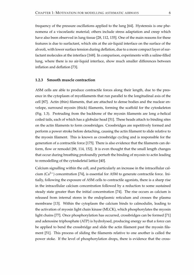
1.2.3 Smooth muscle contraction
ASM cells are able to produce contractile forces along their length, due to the pres-
ence in the cytoplasm of myofilaments that run parallel to the longitudinal axis of the
cell [87]. Actin (thin) filaments, that are attached to dense bodies and the nuclear en-
velope, surround myosin (thick) filaments, forming the scaffold for the cytoskeleton
(Fig. 1.3). Protruding from the backbone of the myosin filaments are long α-helical
coiled tails, each of which has a globular head [51]. These heads attach to binding sites
on the actin filaments to form crossbridges. Crossbridges are repetitively formed and
perform a power stroke before detaching, causing the actin filament to slide relative to
the myosin filament. This is known as crossbridge cycling and is responsible for the
generation of a contractile force [175]. There is also evidence that the filaments can de-
form, flow or remodel [88, 114, 152]. It is even thought that the small length changes
that occur during breathing profoundly perturb the binding of myosin to actin leading
to remodelling of the cytoskeletal lattice [40].
Calcium signalling within the cell, and particularly an increase in the intracellular cal-
cium (Ca2+) concentration [74], is essential for ASM to generate contractile force. Ini-
tially, following the exposure of ASM cells to contractile agonists, there is a sharp rise
in the intracellular calcium concentration followed by a reduction to some sustained
steady state greater than the initial concentration [74]. The rise occurs as calcium is
released from internal stores in the endoplasmic reticulum and crosses the plasma
membrane [13]. Within the cytoplasm the calcium binds to calmodulin, leading to
the activation of myosin light chain kinase (MLCK), which phosphorylates the myosin
light chains [77]. Once phosphorylation has occurred, crossbridges can be formed [71]
and adenosine triphosphate (ATP) is hydrolysed, producing energy so that a force can
be applied to bend the crossbridge and slide the actin filament past the myosin fila-
ment [51]. This process of sliding the filaments relative to one another is called the
power stoke. If the level of phosphorylation drops, there is evidence that the cross-

CHAPTER 1: MOTIVATION FOR MODELLING ASTHMATIC AIRWAYS 7
bridges can remain attached and are capable of maintaining a force, in which case they
are called latch bridges [37]. Further discussion about calcium regulation and the var-
ious pathways involved are beyond the scope of this thesis, with interested readers
directed to [35, 74].
1.3 The asthmatic lung
There are a number of features of the asthmatic lung that are different from a normal
lung. During an asthmatic exacerbation short-term airway inflammation occurs, while
remodelling of the airway wall can occur over longer periods of time, which can lead
to worsening symptoms [17, 178]. There is also evidence that remodelling is observed
early in the development of the disease and is possibly required for the onset of persis-
tent inflammation [32].
1.3.1 Inflammation in human allergic asthma
As described previously, mucus is continuously produced to trap particles that are in-
haled and thereby protects the airways. However, on occasions inhaled allergens may
disrupt the epithelial-cell barrier and cause damage to the airway wall [54]. Upon
initial contact with an antigen, T helper cells, a type of white blood cell, produce Im-
munoglobulin E (IgE) antibodies specific to the allergen, which attach to mast cells.
Upon subsequent contact, the antigen binds to the IgE antibodies and the mast cell
releases proinflammatory mediators such as histamine, cysteinyl leukotrienes and cy-
tokines. This leads to an early allergic response.
The release of the proinflammatory mediators characterises the early allergic response
and results in mucus secretion, ASM contraction and elevated vascular permeability,
which allows cells of the immune system to leave blood vessels [60]. In asthma the
airways may be over-sensitised, which can result in chronic inflammation [144], mu-
cus hypersecretion and airway hyperresponsiveness. Mucus hypersecretion refers to
an excessive production and secretion of mucus. This can contribute towards airway
hyperresponsiveness [148] and plugging of the airways. Airway hyperresponsiveness
refers to smooth muscle cells contracting more readily to a given dose of agonist. These
responses restrict air flow [126] and contribute to a decrease in lung function. Deteri-
oration in lung function can begin within a few minutes, and reach its worst by 30
minutes before improving over several hours [7].
Some individuals who have allergic asthma can also experience a late response be-

CHAPTER 1: MOTIVATION FOR MODELLING ASTHMATIC AIRWAYS 8
tween 6 to 9 hours later. This occurs due to the elevated vascular permeability of the
blood vessels, which dilate and transport a large number of eosinophils to the airway
wall [34]. Eosinophils are a type of white blood cell that are normally absent or low in
number [169]. On arrival, the eosinophils release further proinflammatory mediators,
cytotoxic mediators and cytokines, which results in further vascular leakage, mucus
hypersecretion, smooth muscle contraction plus epithelial shedding [14].
1.3.2 Airway wall remodelling
Damage to the epithelial surface reduces its protective barrier effect and so increases
the likelihood for allergic insult on the airway [11]. In a healthy lung the original struc-
ture of the epithelial cells is restored following damage [143]. However, if the repair
of the damaged epithelium is incomplete this can lead to persistent asthma. Due to
the incomplete repair process, the epithelium produces various growth factors such as
epithelial growth factors, fibroblast growth factors and insulin-like growth factors, that
can contribute towards tissue remodelling [59]. Greater volumes of these factors can
be released in the presence of mechanical stress, chemical and physical injury, virus
infection and interactions with inflammatory cells [59, 137]. There are various ways
in which airway remodelling may occur, leading to a progressive reduction in lung
function [133]. They include the following:
• Goblet cell hyperplasia is the process where goblet cells proliferate abnormally,
not only in the proximal airways, where they are usually found, but also in
the smallest conducting airways (<2mm in diameter), where they are normally
scarce or absent (here the proliferation is known as metaplasia) [147]. As a result
more mucus can be secreted, increasing the likelihood that the airways will be
blocked, or collapse due to elevated surface tension [14].
• Subepithelial fibrosis leads to a thickened basement membrane, due to extracel-
lular matrix including collagen and fibronectin being deposited [11, 145]. This
thickening persists even in patients with well-controlled mild asthma [72].
• ASM cells can increase both in number and size as they undergo hyperplasia
and/or hypertrophy [58]. Usually this mainly affects the large airways, but in
some cases the whole network is affected [14].
• As a damaged airway is repaired, new blood vessels sprout from the existing
vessels, a process called angiogenesis. These airways have been found to be hy-
perpermeable and lead to an increase of oedema [14].

CHAPTER 1: MOTIVATION FOR MODELLING ASTHMATIC AIRWAYS 9
• The layer between the airway smooth muscle and the parenchyma can also
thicken, which may enhance the ability of the ASM to contract by reducing the
effect of lung recoil [165].
1.3.3 Diagnosis and treatment
There is no all-encompassing test for asthma with symptoms common to a range of
disorders. For example, some of the diseases, whose symptoms can be mistaken for
asthma include chronic obstructive pulmonary disease, cystic fibrosis and vocal cord
dysfunction [164]. There are various tests that are used to determine the performance
of the lung, including measuring the forced expiratory volume in one second (FEV1)
and the peak flow in a forced expiration [19]. The results are used to help diagnose for
asthma by comparing with normal values for a person of a particular height, gender,
ethnicity and age [161], with lung function tending to improve for the first 18-20 years
of life before plateauing and then slowly declining [25]. Readings are likely to be lower
in those with asthma, since episodes of inflammation and remodelling can lead to per-
sistent airflow obstruction [23]. A reduction in lung function has been seen in large
studies for all people suffering from asthma, with greater reduction in those with more
severe asthma [136, 142]. The natural decline with ageing is also seen to be accelerated,
although many asthmatics can retain a near normal level of lung function throughout
life with some reversible acute deterioration [151]. Lung function tests can also be used
periodically to highlight any variations and indicate the effectiveness of treatment.
There is also no cure or definitive treatment for asthma. Due to some types of asthma
being allergen-induced, it is possible to reduce the likelihood of attacks by avoiding
contact with the allergen. However, since this is not always possible, or avoidance
alone may not be sufficient, medicines are also required. These can take the form of
preventers or relievers [18, 60]. A common treatment for reducing asthma symptoms is
the use of bronchodilators, which act as relievers. β2-adrenoceptor agonists are inhaled,
either once asthma symptoms appear or shortly before they are expected, with the
agonists attaching to the β2-adrenoceptor on the airway smooth muscle cell, which
leads to ASM relaxation and bronchodilation. Salbutamol and terbutaline are examples
of quick-acting relievers, which restore normal breathing within five to ten minutes and
are effective for about four hours [60]. Formoterol and salmeterol are examples of long-
acting relievers, which act more slowly but can induce bronchodilation for at least 12
hours [131]. Indacaterol is an example of an ultra-long acting reliever, which need only
be taken once every 24 hours [149]. Rather than relieving symptoms, corticosteroids
inhibit the expression of cytokines, chemokines and adhesion molecules, reducing the

CHAPTER 1: MOTIVATION FOR MODELLING ASTHMATIC AIRWAYS 10
inflammation of the airways, thus preventing the onset of asthma symptoms [5].
Bronchial thermoplasty is a more recently developed treatment for severe asthmatics,
that involves transmitting radiofrequency energy to the airway wall to reduce the ASM
mass [30]. Following treatment it has been observed that the frequency of severe exac-
erbations reduced, but lung function tests and hyperresponsiveness measures showed
no significant difference [9].
1.3.4 Experiments on ASM
There has been a large amount of experimental research to understand the processes
behind asthma better. Since the hyper-responsiveness of ASM to certain external stim-
uli, and the associated remodelling of the airway wall, is central to the development
of asthma, research into ASM in particular has widespread clinical significance [82].
One approach that has aided understanding has been an experimental one, involving
the addition of agonists that are known to cause smooth muscle contraction. The re-
sulting isometric force or contraction can be found, so that dose response curves can
be plotted [12, 33, 42, 132, 182]. However, in vivo the length of the ASM within the
airway will vary continuously due to tidal breathing and periodic deep inspirations.
It has also long been known that a deep inspiration (DI) has a bronchodilatory effect
on constricted airways of normal subjects [122], while for asthmatics a DI may have a
reduced bronchodilatory effect, may do nothing, or may even result in additional con-
traction [107]. Due to the importance of understanding the difference between asth-
matics and non-asthmatics, many experiments have been designed to investigate how
dynamic stretching affects the level of bronchocontraction.
A number of experiments have been carried out on tracheal tissue strips, dissected from
a variety of different species, with most of the extracellular matrix removed [8, 43, 174].
Agonist is applied to the strips, which are stretched and clamped at each end and
allowed to reach maximum isometric force. Length oscillations are then prescribed
with the resulting force along the strip being recorded, from which force-length loops
can be plotted [8, 43]. These studies showed that the introduction of length oscilla-
tions reduces the mean contractile force, with the size of the reduction proportional
to the amplitude of the oscillations. Similar experiments were carried out on airways
dissected from the parenchyma by applying volume oscillations [50], for which in-
creased oscillation amplitude again resulted in reduced contractile force. Due to the
questions over the relevance of length/volume oscillations of ASM in vivo, further ex-
periments have been carried out on tissue strips, where force rather than length was
prescribed [104, 129]. The size of the force exerted on the strip was chosen to try to

CHAPTER 1: MOTIVATION FOR MODELLING ASTHMATIC AIRWAYS 11
mimic the force that a ring of ASM would experience when physiological transpul-
monary pressures are applied to the lung. The Young Laplace approximation and the
semi-empirical expressions of Lambert et al. [96, 98] were used to approximate the force.
Results showed that increasing the amplitude of the transpulmonary pressure led to a
reduction in the mean force along the strip and an increase in the mean length of the
strip.
In the last few years, experiments have also been developed to prescribe physiological
transmural pressures to airways dissected from the parenchyma [103, 125]. In contrast
to the strip experiments, initial results on bovine airways demonstrated little reduction
in contraction when tidally oscillated compared to when static [103]. Having initially
questioned whether the result was species specific [124], Noble et al. went on to show
that similar results are found with human airways [125]. A number of editorials were
published that discussed questions raised by these differences [100, 102, 124]. LaPrad et
al. [103] pose the following questions: are appropriate loading conditions being applied
to the ASM strips, which are based on static airway wall models, while the experiments
on the airway are dynamic; how do the oscillatory strains measured in the airway com-
pare to the actual strain in the ASM; do the geometry and structure of the airway wall
provide a unique mechanical environment, thus producing the differences observed?
In a recent paper, Noble et al. [101] obtained a number of surgically removed bronchial
segments from subjects with or without known asthma. They found some evidence
that ASM mass was a key reason for the greater contraction in segments from asth-
matics and, independent of diagnosis for asthma, if segments were initially equally
contracted, they would respond in the same way to deep inspirations. They therefore
concluded that the maximum contraction and the reduced bronchodilatory response
to deep inspirations in asthma are independent, and that there does not exist some
impairment in asthmatic tissue that reduces the effectiveness of deep inspirations.
Another way to study the ASM is through the use of precision-cut lung slices [12],
which allows contacted airways embedded in parenchyma to be studied. Recently
Lavoie et al. [105] developed a technique that allows for oscillatory stretching of the
surrounding parenchyma, to simulate breathing. They also found that the amount of
stretch experienced by the ASM was important in determining the level of reversal of
bronchoconstriction, with both the amplitude of the oscillations and the severity of the
initial contraction being important factors.

CHAPTER 1: MOTIVATION FOR MODELLING ASTHMATIC AIRWAYS 12
1.3.5 Summary
The airways are integral in the transport of oxygenated air into the lung and the re-
moval of carbon dioxide. In asthma these processes can be hindered as the airways nar-
row, due to an exaggerated response to inhaled allergens, characterised by extra mucus
secretion and ASM contraction. The contractile force produced by the ASM depends
on calcium signalling and the attachment of cycling crossbridges between myosin and
actin filaments within the ASM cells. Another important feature is the long-term re-
modelling of the airway wall, including increased ASM mass, which can lead to the
persistence of inflammation and asthma symptoms. Due to the nature of asthma —
with contributions ranging from calcium signalling right up to the deformation of the
lung as a whole — there is a wide spectrum of length scales that are important. Due to
the importance of both inflammation and airway remodelling there are also multiple
timescales involved.
Between asthma sufferers there are large variations in the triggers and symptoms and
there is no definitive treatment or cure. In order to try to understand ASM more fully,
a range of experiments have been carried out with various geometries and protocols,
but the results from the different experiments have not been consistent. Experiments
have been carried out on tissue strips, dissected airways and lung slices, where length
oscillations or pressure oscillations have been prescribed. The results are very difficult
to compare given the potentially different strains being imposed, existence (or lack) of
parenchymal tethering and changes in geometry of the ASM. A mathematical model
will enable us to understand how different factors contribute. Some of the things that
could be taken into account by the model include:
• the thickness of the airway wall due to remodelling;
• the level of agonist applied to the airway;
• the effect collagen has on the airway;
• how passive forcing alters the level of contraction;
• how ASM responds differently in a strip compared to in an airway.
In the following sections we shall review existing mathematical models, indicating ar-
eas for us to further investigate, before going on to review some of the mathematical
techniques that will be required to carry out the modelling.

CHAPTER 1: MOTIVATION FOR MODELLING ASTHMATIC AIRWAYS 13
2k
CyclingLatch
1
6
Crossbridge Crossbridge
Mp, n
AM, n AMp, n
k
k
k
M, n
5
A B
CD
k k k 347
Figure 1.4: Four state crossbridge model by Hai and Murphy [52]. M refers to the
myosin filament. A refers to the actin filament, which a crossbridge has
attached to. p indicates that a crossbridge has been phosphorylated. The
ns refer to the fraction of crossbridges in each of the states.
1.4 Review of mathematical models
We begin by considering models that describe the crossbridge dynamics before moving
on to previous models of asthmatic airways.
1.4.1 Crossbridge mechanics
In the 1980s a model for crossbridge dynamics of smooth muscle was introduced
by Hai and Murphy [52] consisting of four states. Myosin crossbridges can be de-
tached and unphosphorylated, M, detached and phosphorylated, Mp, attached and
phosphorylated, AMp, or attached and dephosphorylated, AM. The phosphorylated
crossbridges are called cycling crossbridges due to the fact that they are rapidly attach-
ing and detaching. The attached-dephosphorylated crossbridges detach more slowly
and are known as latch bridges. The possible reactions from the Hai-Murphy model
are shown in figure 1.4. The rates at which unattached crossbridges are phosphory-
lated and dephosphorylated are k1 and k2, respectively. k1 is related to the calcium
concentration, while k2 is related to the level of agonist. Similarly the attached cross-
bridges are phosphorylated and dephosphorylated at rates k6 and k5. Phosphorylated
crossbridges attach at a rate k3 and detach at a rate k4. Dephosphorylated crossbridges
detach at a rate k7 (experiments have shown that the crossbridges must be phosphory-
lated in order to attach).
By considering nA, nB, nC and nD, representing the fraction of crossbridges in states
M, Mp, AMp and AM, respectively, in the chemical kinetic scheme (Fig. 1.4), Hai and
Murphy [52] derive four coupled ordinary differential equations, which in vector form
becomedn(t)
dt= Q(t)n(t), (1.4.1)

CHAPTER 1: MOTIVATION FOR MODELLING ASTHMATIC AIRWAYS 14
where n is a vector of the crossbridge state fractions and Q is the transition matrix given
by
Q =
−k1 k2 0 k7
k1 −k2 − k3 k4 0
0 k3 −k5 − k4 k6
0 0 k5 −k6 − k7
. (1.4.2)
In order to take into account load fluctuations on the rates of attachment and detach-
ment, Mijailovich et al. [116] and Fredberg et al. [44] integrated the four-state model
of Hai and Murphy [52] with the sliding filament theory of muscle contraction devel-
oped by Huxley [68]. The adapted model is referred to as HHM theory. The rates
of phosphorylation and dephosphorylation are unchanged, but now phosphorylated
crossbridges attach at a rate fp(x) and detach at a rate gp(x), and dephosphorylated
crossbridges detach at a rate g(x). These rates depend on x, where x is the distance
along the actin filament to the binding site (Fig. 1.5). Attachment is assumed only to be
possible if the actin binding site is in the interval 0 < x < h, where h is the power-stroke
length. Detachment can occur at any x. If x < 0, the rate of detachment is assumed
to be much more likely, so that the crossbridges do not stay attached and resist further
contraction. If x > h, the rate of detachment is assumed to increase as x increases, to
take into account the fact that the crossbridges are more likely to snap off, the more they
are stretched. The attachment and detachment rates may be described as follows [116]:
fp(x) =
0, x < 0
fp1x/h, 0 ≤ x ≤ h
0, x > h,
(1.4.3a)
gp(x) =
gp2, x < 0
gp1x/h, 0 ≤ x ≤ h
(gp1 + gp3)x/h, x > h,
(1.4.3b)
g(x) =
g2, x < 0
g1x/h, 0 ≤ x ≤ h
(g1 + g3)x/h, x > h.
(1.4.3c)
The way that the HHM model is solved depends on what is assumed about the distri-
bution of the actin binding sites. Firstly, it may be assumed that the distance between
the actin binding sites is much larger than the region within which the crossbridges can
attach, meaning that there is only ever one binding site that a crossbridge can attach to.

CHAPTER 1: MOTIVATION FOR MODELLING ASTHMATIC AIRWAYS 15
AMpAM
CyclingLatch
1
2
Crossbridge Crossbridge
k
k
k
k 5
6
Mp
fppgg
Myosin
Actin
Crossbridge
x
(x)(x)(x)
M (b)(a)
Figure 1.5: (a) The four-state crossbridge HHM model. The rate of attachment and de-
tachment now depend on x. (b) x is the distance reached by a crossbridge
to an actin binding site.
In this case there is the following conservation law:
nA(x, t) + nB(x, t) + nC(x, t) + nD(x, t) = 1. (1.4.4)
There is the following system of partial differential equations:
∂n∂t− v
∂n∂x
= Qn, (1.4.5)
where v is the velocity of the actin relative to the myosin and is taken to be positive
during contraction, n is a vector of the crossbridge state fractions and Q is the transition
matrix given by
Q(x, t) =
−k1 k2 0 g(x)
k1 −k2 − fp(x) gp(x) 0
0 fp(x) −k5 − gp(x) k6
0 0 k5 −k6 − g(x)
. (1.4.6)
Secondly, it can again be assumed that the distance between binding sites ∆x is greater
than h, but that as the actin filament slides occupied binding sites can enter the re-
gion of attachment. The displacement associated with unattached crossbridges is the
distance to the binding site with which it could bind, and the density of unattached
crossbridges is defined only in the region 0 < x < ∆x. While it is only possible for
crossbridges to attach in the region 0 < x < h, due to contraction and extension of the
muscle, it is possible that there exist attached crossbridges in the region −∞ < x < ∞.
Whenever an attached crossbridge detaches, it is assumed that it immediately becomes
an unattached crossbridge with position x + i∆x, where i is the smallest integer for
which x + i∆x > 0. The evolution equations for the densities of each of the four types

CHAPTER 1: MOTIVATION FOR MODELLING ASTHMATIC AIRWAYS 16
of crossbridges are [80]
∂nA
∂t− v(t)
∂nA
∂x= k2nB − k1nA +
∞
∑i=−∞
g(x− i∆x)nD(x− i∆x, t), (1.4.7a)
∂nB
∂t− v(t)
∂nB
∂x= k1nA − (k2 + fp(x))nC +
∞
∑i=−∞
gp(x− i∆x)nC(x− i∆x, t), (1.4.7b)
∂nC
∂t− v(t)
∂nC
∂x= k6nD + fp(x)nB − (k5 + gp(x))nC, (1.4.7c)
∂nD
∂t− v(t)
∂nD
∂x= k5nC − (k6 + g(x))nD. (1.4.7d)
It is also required that as the muscle contracts or lengthens, the flux of unattached
crossbridges at x = 0 and at x = ∆x are equal, so that [80]
∂nA(0, t)∂x
=∂nA(∆x, t)
∂x,
∂nB(0, t)∂x
=∂nB(∆x, t)
∂x. (1.4.8)
Now if (1.4.7a)-(1.4.7b) are evaluated at x + i∆x and summed over all i and then also
add (1.4.7c) and (1.4.7d) the following conservation law is found [116]:
nA(x, t) + nB(x, t) +∞
∑i=−∞
[nC(x + i∆x, t) + nD(x + i∆x, t)] = 1, (1.4.9)
for 0 < x < ∆x. More complex models could also be derived, for which ∆x < h or
there is a continuous distribution of binding sites.
An alternative to using the Huxley model [68], to adapt the Hai-Murphy model [53],
would be to use a variation of the model of Marcucci and Truskinovsky [110, 111].
Rather than considering the kinetics of the power stroke in terms of jump processes,
the energy of the crossbridges is considered and is assumed to evolve stochastically. In
brief, they modelled a crossbridge as a spring and a bistable element in series (Fig. 1.6).
An attached crossbridge starts off with the end of the spring in the well of the bistable
element with the greater potential energy. When the crossbridge performs a power-
stroke, the spring stretches and its end moves into the second well. Given a sufficient
stimulus the crossbridge can also step along a ratchet, that represents the actin filament.
The system cycles spontaneously between the different states, driven by external noise,
so that over long timescales (and on average) the behaviour is similar to the determin-
istic Hai-Murphy model. An advantage of the stochastic system is that arrays of wells
and ratchets can be studied to understand force-length-velocity relationships arising
from different spatial arrangements of sarcomeres in the cell.
1.4.2 Existing models for asthmatic airways
An overview of relevant previous models of the asthmatic airway are now presented.

CHAPTER 1: MOTIVATION FOR MODELLING ASTHMATIC AIRWAYS 17
(a)bistable element
ratchet
spring(b) (c)
Figure 1.6: Diagram of the setup used by Marcucci and Truskinovsky [111] to model
crossbridge mechanics in skeletal muscle. The model consists of a spring,
a bistable element and a Brownian ratchet. (a) The spring starts off in the
higher potential well of the bistable element. (b) Following a power stroke,
the spring moves to the lower potential well. (c) The crossbridge can step
along the ratchet, with the spring returning to the higher potential well of
the bistable element. The process can repeat.
While considering expiratory flow, Lambert et al. [98] developed a model for human
airways, to describe the relationship between α, the airway area normalised by the
maximum airway area, and P, the transmural pressure. The model was based on the
data of Weibel [176] and Hyatt et al. [69] and consisted of two rectangular hyperbolae,
so that
α =
α0
(1− Pα′0
α0n1
)−n1if P ≤ 0
1− (1− α0)(
1 + Pα′0(1−α0)n2
)−n2if P > 0.
(1.4.10)
There are five parameters, the maximum airway area, α0 and α′0, the normalised area
and slope when P = 0, and n1 and n2. The value of these parameters are set for each
airway generation. Lambert and Wilson [97] extended this work to take into account
smooth muscle contraction. They expressed the transmural pressure as the sum of
three terms: the elastic recoil pressure due to the distortion of the airway wall given by
(1.4.10); a recoil pressure due to distortion of the parenchyma; and a pressure due to
the contraction of ASM. The Laplace law for thin cylinders is used to assume that the
pressure due to the muscle is of the form
Pm =Frm
, (1.4.11)
where rm is the radius to the muscle and F is active force, that can be modelled to take
into account the level of muscle activation, muscle length and length history.
In recent years a number of further models of the asthmatic airway have been pub-
lished. Wang et al. [173] assumed the ASM cells formed a ring that was embedded in a
linearly elastic, isotropic, homogeneous sheet. Assuming axisymmetry they found that
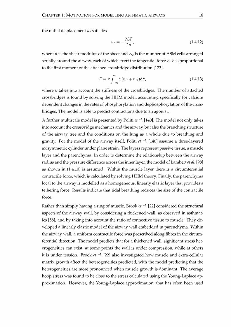
CHAPTER 1: MOTIVATION FOR MODELLING ASTHMATIC AIRWAYS 18
the radial displacement ur satisfies
ur = −NcF2µ
, (1.4.12)
where µ is the shear modulus of the sheet and Nc is the number of ASM cells arranged
serially around the airway, each of which exert the tangential force F. F is proportional
to the first moment of the attached crossbridge distribution [173],
F = κ∫ ∞
−∞x(nC + nD)dx, (1.4.13)
where κ takes into account the stiffness of the crossbridges. The number of attached
crossbridges is found by solving the HHM model, accounting specifically for calcium
dependent changes in the rates of phosphorylation and dephosphorylation of the cross-
bridges. The model is able to predict contractions due to an agonist.
A further multiscale model is presented by Politi et al. [140]. The model not only takes
into account the crossbridge mechanics and the airway, but also the branching structure
of the airway tree and the conditions on the lung as a whole due to breathing and
gravity. For the model of the airway itself, Politi et al. [140] assume a three-layered
axisymmetric cylinder under plane strain. The layers represent passive tissue, a muscle
layer and the parenchyma. In order to determine the relationship between the airway
radius and the pressure difference across the inner layer, the model of Lambert et al. [98]
as shown in (1.4.10) is assumed. Within the muscle layer there is a circumferential
contractile force, which is calculated by solving HHM theory. Finally, the parenchyma
local to the airway is modelled as a homogeneous, linearly elastic layer that provides a
tethering force. Results indicate that tidal breathing reduces the size of the contractile
force.
Rather than simply having a ring of muscle, Brook et al. [22] considered the structural
aspects of the airway wall, by considering a thickened wall, as observed in asthmat-
ics [58], and by taking into account the ratio of connective tissue to muscle. They de-
veloped a linearly elastic model of the airway wall embedded in parenchyma. Within
the airway wall, a uniform contractile force was prescribed along fibres in the circum-
ferential direction. The model predicts that for a thickened wall, significant stress het-
erogeneities can exist; at some points the wall is under compression, while at others
it is under tension. Brook et al. [22] also investigated how muscle and extra-cellular
matrix growth affect the heterogeneities predicted, with the model predicting that the
heterogeneities are more pronounced when muscle growth is dominant. The average
hoop stress was found to be close to the stress calculated using the Young-Laplace ap-
proximation. However, the Young-Laplace approximation, that has often been used

CHAPTER 1: MOTIVATION FOR MODELLING ASTHMATIC AIRWAYS 19
to model narrowing airways (e.g. (1.4.11)), averages out the heterogeneity that is pre-
dicted to exist.
An alternative to the elastic models would be viscoelastic models. In order to model
the hysteresis observed when length oscillations are applied to an unactivated strip of
ASM, Bates et al. [8] assumed that the passive component of the material could be de-
scribed using a spring parallel to a spring and dashpot in series. A similar arrangement
of springs and dashpots that were in series with the force generator, was assumed to
describe the active component of the material. With such a model they were able to get
a reasonable fit to the data from the strip experiment. While this model is for a strip of
ASM, a similar model could be used for an airway.
1.4.3 Other relevant models
Various techniques have also been used to model the lung parenchyma. A number of
strain-energy functions have been proposed including those of Lai-Fook et al. [90, 92],
Stamenovic and Wilson [159] and Fung et al. [45]. However, each of these are quite
complex, depending on six, six and four parameters respectively. Alternatively, Mead
et al. [113] and Takishima and Mead [167] assumed a network of hexagonally arranged
springs. However, it has been shown that predictions differ when the parenchyma
is modelled as a network of hexagonally arranged springs or as an elastic contin-
uum [108], and by comparing the model predictions to the displacement observed in
a contracting lung slice, Ma et al. [109] showed that the continuum approach is supe-
rior. When modelling lung ventilation, further models were developed consisting of
an elastic or viscoelastic porous material [99, 130, 153].
Buckling of airways is also an important feature, although beyond the scope of this
thesis. For models of mucosal folding the reader is pointed to the work of Wiggs et
al. [179] and the simplified model of Donovan and Tawhai [38]. A model that takes
into account growth, by increasing the mass in the radial or circumferential direction,
or a combination of the two, is presented by Moulton and Goriely [119]. For a model
taking into account the surface-tension-driven instabilities due to the surfactant and
liquid that lines the airways, see the work of Heil et al. [56].
1.4.4 Extending the current models
In this thesis we will extend the existing models for the asthmatic airway. Given the
interesting model predictions of Brook et al. [22] for a thickened airway wall as it con-
tracts, we will extend this work to allow for finite deformations. This will be possible

CHAPTER 1: MOTIVATION FOR MODELLING ASTHMATIC AIRWAYS 20
by implementing nonlinear elasticity with fibre-reinforcement within the airway wall.
The model of Brook et al. [22] will also be extended by using HHM to determine the
contractile force as in [140, 173], so that time-dependent solutions can be investigated.
By applying oscillatory boundary conditions, in order to mimic breathing, comparisons
will be made to experimental data that investigates the effect of tidal breathing on bron-
choconstriction. To take into account that the lung parenchyma is strongly viscoelastic,
a simple viscoelastic model will also be developed that can be compared to the elastic
model.
1.5 Review of mathematical techniques
A review is now presented of some of the mathematical techniques required to develop
the model of the airway wall embedded in parenchymal tissue. Nonlinear elasticity is
introduced in section 1.5.1, including a discussion on strain energy functions and an
introduction to the incorporation of anisotropy and active force within fibres. Some
simple models for a linear viscoelastic material are reviewed in Sec. 1.5.2.
1.5.1 Nonlinear elasticity
If X and x denote the position vector of a material point in the reference and deformed
configurations, the deformation gradient tensor F, defined by
F = Gradx or Fij =∂xi
∂Xj, (1.5.1)
maps the deformation from the reference to the current configuration. The deformation
gradient tensor can split in the following ways [36]:
F = RU, F = VR, (1.5.2)
where R is a proper orthogonal rotation tensor, and U and V are positive definite sym-
metric tensors known as the right and left stretch tensors. Two other important sym-
metric tensors are the right and left Cauchy-Green deformation tensors that are related
to the square of the stretch and are respectively defined as
C = FTF = U2, B = FFT = V2. (1.5.3)
B and C depend on the coordinate system that is used; however, stress invariants are
independent of the coordinate system that is used. The isotropic invariants of C are
given by
I1 = tr(C), I2 =12
[tr(C)2 − tr
(C2)] , I3 = det(C). (1.5.4)

CHAPTER 1: MOTIVATION FOR MODELLING ASTHMATIC AIRWAYS 21
The isotropic invariants of B are defined analogously.
Now while isotropic materials have the same material properties in all directions, in or-
der to include extensible fibres to model the collagen and ASM, an anisotropic material
is required. Assuming that there are two sets of densely-distributed fibres with pre-
ferred directions M1 and M2, there are the following additional strain invariants [128]:
I4 = M1 · (CM1), I5 = M1 · (C2M1), I6 = M2 · (CM2),
I7 = M2 · (C2M2) and I8 = M1 · (CM2). (1.5.5)
I4 and I6 represent the square of the stretch in the directions M1 and M2, respec-
tively [63]. The other invariants have no simple physical interpretation.
The second Piola-Kirchoff stress is given by [66]
S = 2∂W∂C
= 23
∑i=1
Wi∂Ii
∂C(1.5.6)
where W is the strain-energy function for the material and Wi ≡ ∂W/∂Ii. There-
fore [128], S is given by
S =2[
W1I + W2 (I1I− C) + W3 I3C−1 + W4M1 ⊗M1 + W5(M1 ⊗ CM1 + CM1 ⊗M1)
+ W6M2 ⊗M2 + W7(M2 ⊗ CM2 + CM2 ⊗M2)
+W8
2(M1 ⊗M2 + M2 ⊗M1)
], (1.5.7)
where I is the identity tensor and C−1 = F−1F−T is the inverse of C.
It is necessary to find the Cauchy stress tensor, τ, which is given in terms of the second
Piola-Kirchoff stress tensor S as follows:
τ =FSFT
J, (1.5.8)
where
J = det(F) =√
I3 (1.5.9)
is the ratio between the current volume and the undeformed volume. Using (1.5.7) and
(1.5.8), the Cauchy stress tensor is
τ =2J
[W1B + W2
(I1B− B2) + I3W3I + W4m1 ⊗m1 + W5(m1 ⊗ Bm1 + Bm1 ⊗m1)
+ W6m2 ⊗m2 + W7(m2 ⊗ Bm2 + Bm2 ⊗m2)
+W8
2(m1 ⊗m2 + m2 ⊗m1)
], (1.5.10)
where m1 = FM1 and m2 = FM2 are the directions of the two sets of fibres in the
current configuration. Conservation of momentum requires ∇ · τ = 0, where differen-
tiation is with respect to the deformed configuration [155].

CHAPTER 1: MOTIVATION FOR MODELLING ASTHMATIC AIRWAYS 22
1.5.1.1 Strain-energy functions
Strain-energy functions relate the energy put into the material with the resulting strain.
So that the function is independent of the coordinate system used, the function depends
on the stress invariants. There is a lot of freedom in the choice of the function, but for
the stress to vanish in the reference configuration it is required that(
∂W∂I1
+ 2∂W∂I2
+∂W∂I3
) ∣∣∣∣I1=I2=3,I3=1
= 0. (1.5.11)
Some commonly used strain energy functions are now briefly described.
A simple strain-energy function for incompressible materials is the neo-Hookean func-
tion that depends only on I1 and the shear modulus µ so that
W =µ
2(I1 − 3). (1.5.12)
A slightly more complicated version is that of a Mooney-Rivlin material, which satisfies
W = c1(I1 − 3) + c2(I2 − 3), (1.5.13)
where c1 and c2 are material constants.
The following extension of the Mooney-Rivlin model is given in [62], to allow for the
material to be compressible:
W = αµ
2(I1 − 3) + (1− α)
µ
2(I2 − 3) + c(J − 1)2 − d log J, (1.5.14)
where α ∈ [0, 1] is an interpolation parameter and the terms containing J were pro-
posed by Ciarlet and Geymonat [26]. c is a material parameter and d is a parameter that,
assuming the reference configuration is stress free, using (1.5.11) yields d = µ(2− α)/2.
This is an example of a strain-energy function where the isochoric component, that
deals with volume preserving deformations, and the volumetric component, that deals
with volume changes, are coupled. An alternative is split the function into separate
volumetric and isochoric components, Wvol and Wiso respectively, such that
W(J, I1, I2) = Wvol(J) + Wiso(I1, I2), (1.5.15)
where Ii = Ii/I3 for i = 1, 2. An example of an equation for Wvol is the Ogden model
for compressible (rubber-like) materials, where
Wvol = κβ−2(
β log J +1Jβ− 1
). (1.5.16)
κ is the bulk modulus and β is a positive material parameter.

CHAPTER 1: MOTIVATION FOR MODELLING ASTHMATIC AIRWAYS 23
As neo-Hookean and Mooney-Rivlin materials are stretched, smaller increases in force
are required to stretch the material further. An example of an isotropic strain-energy
function that can produce strain-stiffening (so that as the material stretches, larger in-
creases in force are required to stretch the material further) is the Ogden strain-energy
function. This depends on the principal stretches, λ1, λ2 and λ3, of F rather than the
strain invariants and is given by
W = 2µλ
β1 + λ
β2 + λ
β3 − 3
β, (1.5.17)
where µ and β are positive constants [127]. This function is used when modelling in-
compressible rubber. Holzapfel et al. [61] discussed other examples, before developing
a new model. Instead of simply assuming an isotropic material, they based their model
on the theory of the mechanics of fiber-reinforced composites [157] and assumed that
the underlying material is isotropic but there are also anisotropic fibres. The strain-
energy function is split into an isotropic part, Wi and an anisotropic part, Wani so that
W = Wi(I1, I2, I3) + Wani(I1, I2, I3, I4, I5, I6, I7, I8). (1.5.18)
For simplicity when considering an incompressible material, Holzapfel et al. [61] de-
scribe the isotropy by I1 alone and the anisotropy by I4 and I6 so that
W(I1, I4, I6) = Wi(I1) + Wani(I4, I6). (1.5.19)
For the isotropic component they assume a neo-Hookean material, while modelling
Wani as
Wani(I4, I6) =k1
2k2∑
i=4,6H(Ii − 1)
exp
[k2(Ii − 1)2]− 1
, (1.5.20)
where k1 > 0 is a stress-like parameter while k2 > 0 is a dimensionless parameter, that
can be used to alter the amount of strain-stiffening. H(Ii − 1) is the Heaviside function
so that the fibres only contribute when stretched. According to this model, for small
stretches the fibres provide little resistance, however, as the fibres stretch the amount
of energy required to stretch them further increases exponentially. Gasser et al. [47]
extended (1.5.20) to also allow for some dispersion of the fibre directions.
1.5.1.2 Including active fibres
In order to take into account the contractile forces produced by the ASM, active forcing
can be applied along fibres. As described by Ambrosi and Pezzuto [3], there are two
ways in which active stress can be included into a continuum body; either a multiplica-
tive decomposition of the deformation gradient tensor is used or an active component

CHAPTER 1: MOTIVATION FOR MODELLING ASTHMATIC AIRWAYS 24
is added to the stress. In the multiplicative setup
F = FaFe, (1.5.21)
where Fa is the active contribution and Fe is the elastic deformation that ensures that
the material remains compatible [3], meaning that no gaps or overlaps develop in the
deformation. To take into account the orientation of fibres, Fa can take the form
Fa = I− γm1 ⊗m1, (1.5.22)
where γ ∈ (0, 1) and m1 is the current orientation of the fibres [3]. Examples where the
multiplicative method is used are [123, 166].
Using the additive setup the Cauchy stress tensor and the strain-energy function can
be split into passive and active components, so for example
τ = τp + τa, (1.5.23)
where τp gives the passive stress and τa gives the active stress. The general form for
the active component, in the case that the orientation of the fibres is taken into account,
is [3]
τa =f (I4)
J(m1 ⊗m1) . (1.5.24)
There have been a number of suggestions for the form of f (I4), each of which include
a function A, to take into account the level of activation, and the fibre stretch λ. When
modelling vascular smooth muscle Rachev and Hayashi [141] used the following form:
f (I4) = Aλ
(1−
(λm − λ
λm − λ0
)2)
, (1.5.25)
where λm is the stretch at maximum activation and λ0 is the stretch when activation
ceases. Alternatively, when modelling contracting myocytes, Tracqui and Ohayon [172]
let
f (I4) = A(Ca2+) exp(
(λm − λ)2
a
), (1.5.26)
where a is a positive parameter and λm again represents the stretch at maximum acti-
vation. Here, a Hill function is used to describe the contribution of the calcium concen-
trations to A. Again, in modelling vascular smooth muscle, Zulliger et al. [185] let
f (I4) = A (λ− 1) . (1.5.27)
Further models have coupled the chemical state model of Hai and Murphy [52]
(Sec. 1.4.1) with a mechanical model. Models for smooth muscle cells and vessels in
arteries were introduced by Yang et al. [183, 184]. Stålhand et al. [158] developed these

CHAPTER 1: MOTIVATION FOR MODELLING ASTHMATIC AIRWAYS 25
models to enable the coupling of the crossbridge mechanics to a continuum mechan-
ics model. Two further models coupled to the model of Hai Murphy [52] are those of
Kroon [83] and Murtada et al. [120].
Kroon [83] considers that the strain energy function can be split into an active compo-
nent, Wa, and a passive component, Wp, modelling the active component by consider-
ing a spring in series with a dashpot. This takes into account the relative sliding of the
myosin and actin filaments, which are assumed to be rigid, and the elastic stretching of
the attached crossbridges. The stretch of the contractile unit is given by
λ f = λsλe, (1.5.28)
where λs is the stretch due to the sliding of the filaments and λe is the stretch due to the
elastic stretching of the crossbridges (Fig. 1.7). Kroon assumes the active component to
the strain-energy function satisfies
Wa =µ f
2(nC + nD)
(λ2
f
λ2s− 1
)2
, (1.5.29)
where µ f is related to the stiffness of the crossbridges and the number of contractile
units per unit area. The following evolution equation is used to update λs, taking into
account Te, the active stress caused by the attached crossbridges, and ∂Wa∂λs
, the resistance
to filament sliding:
vλs = Te − ∂Wa
∂λs, (1.5.30)
where v is a viscous damping parameter. Since contraction relates to λs < 0, Te < 0. In
prescribing Te it was assumed that there are three possibilities: the cycling crossbridges
(nC) provide a force that is greater than the resistance to sliding so the muscle contracts;
the cycling crossbridges are not strong enough to lead to contraction, but with the latch
bridges (nD) they resist backsliding; the crossbridges are unable to resist backsliding
and the latch bridges detach. Te is thus prescribed as follows [83]:
Te =
−υCnC, if − ∂Wa∂λs
< υCnC,
∂Wa∂λs
, if υCnC ≤ − ∂Wa∂λs
≤ υCnC + υDnD,
−υCnC, if υCnC + υDnD < − ∂Wa∂λs
,
(1.5.31)
where υC and υD are material parameters relating to the driving force of the phospho-
rylated crossbridges and passive resistive strength of the latch bridges. In a follow-up
paper Kroon [84] developed the model to include dispersion of the orientation of the
filaments.
A similar model was developed by Murtada et al. [120]. They first found an expression
for the (averaged) first Piola-Kirchoff stress acting on the contractile units Tf , motivated

CHAPTER 1: MOTIVATION FOR MODELLING ASTHMATIC AIRWAYS 26
L L
λe
sliding
elongationcross−bridge
deformation
myosindense body actin crossbridge
L
L λeλ
Lλ
Lλ
λ s
s
s
s
λ f
Figure 1.7: Diagram of the deformation of the contractile unit. The deformation is
composed of a stretch, λs caused by the actin filaments sliding past the
myosin during contraction and a stretch, λe caused by the crossbridges
stretching. In the reference configuration the unit has length L, while in
the deformed state it has length Lλsλe. Adapted from [120].
by considering the attached crossbridges. The total number of attached crossbridges
within a contractile unit is (nC + nD)ρ, where ρ is the number of available crossbridges,
which is assumed to remain constant. Considering the change of length parallel to the
filaments, each of the crossbridges have stiffness E f , while the actin and myosin fila-
ments are assumed to be rigid. If there are N f contractile units per unit area, summing
over all the attached crossbridges, the resulting stretch of the crossbridges is given by
λe = 1 +Tf
Lλs(nC + nD)E f ρN f, (1.5.32)
where L is the reference length of a contractile unit. From (1.5.28) and (1.5.32)
Tf = µa(nC + nD)λs(λe − 1) = µa(nC + nD)(λ f − λs), (1.5.33)
where µa = LρE f N f .
The following strain-energy function is found by integrating (1.5.33) with respect to λ f :
Wa =µa
2(nC + nD)(λ f − λs)2. (1.5.34)
Murtada et al. [120] also assume a slightly different form for the evolution equation
to Kroon [83], letting υC = υD and assume that the latch bridges are able to resist

CHAPTER 1: MOTIVATION FOR MODELLING ASTHMATIC AIRWAYS 27
elongation, so that
Te = −υC(nC + nD), if υC(nC + nD) < −∂Wa
∂λs. (1.5.35)
Once again this work was extended to allow for the dispersion of filaments [121].
Instead of using the Hai-Murphy model [52], the HHM model could be used ([140,
173] use the HHM model but assume linear elasticity). Whereas with the Hai-Murphy
model [52] the number of attached crossbridges will tend towards a steady state unless
the rate parameters are altered, with the HHM model passive forcing can alter the
distribution, due to the x dependence in the rate parameters. The HHM model also
takes into account the velocity of the relative sliding of the myosin and actin filaments,
so there is no need for a separate evolution equation, and the number and position of
each of the attached crossbridges are updated at each timestep.
While many of these models assume that the number of crossbridges available for bind-
ing is constant, for finite displacements the number available will vary. There have been
a number of approaches to try to overcome this. One approach is to match up to data
by using producing a phenomenological model as used by Schmitz and Böl [150] or
Politi et al. [140] to enable a certain stretch at which the active forcing is greatest. Politi
et al. multiply the force given by (1.4.13) by the following factor:
fl = sin(
πr2rmax
)3
, (1.5.36)
where rmax is the lumen radius at which the force is greatest. Alternatively Kroon [85]
considers how the overlap length of the myosin and actin filaments varies and so the
number of crossbridges available. The model of Brook and Jensen [21] also considers
the change in the number of crossbridges available. They do so by considering both the
overlap length and how the filaments are able to remodel as the length of the smooth
muscle cells changes.
1.5.2 Linear Viscoelasticity
Elastic materials deform instantaneously to a new equilibrium state when stresses are
applied to them, returning to the initial state when the stresses are removed, while vis-
cous materials deform indefinitely under an applied load. Viscoelastic materials exhibit
a mixture of these properties. Viscoelastic materials will be referred to as viscoelastic
solids or liquids depending on how they act at long timescales. In a solid the elastic
properties dominate at large time, while in a fluid the viscous properties dominate.
When stress is increased on a viscoelastic material there will be an immediate change
in the strain followed by a time-dependent increase in strain, known as creep. At large

CHAPTER 1: MOTIVATION FOR MODELLING ASTHMATIC AIRWAYS 28
times the strain of viscoelastic solids will tend to some equilibrium, however viscoelas-
tic fluids will strain indefinitely [138].
Increasing the strain will initially cause the stress to increase but then it will reduce over
some time scale. This is known as stress relaxation [138]. The stress in a viscoelastic
solid will reach an equilibrium greater than zero, while the stress in a viscoelastic fluid
will tend to zero.
Hysteresis is observed in viscoelastic materials when a sinusoidal force is applied to
the material. For an elastic material the strain curve is in phase with the forcing curve,
while the curves are out of phase by π/2 in a viscous material. For a viscoelastic mate-
rial the strain lags behind by a phase angle between zero and π/2 [93].
1.5.2.1 Standard Linear solid model
Some simple one-dimensional viscoelastic models, which incorporate springs and
dashpots so that both elastic and viscous properties can be accounted for, are now con-
sidered. The relationship between stress, σ, and strain, ε, in a linear spring is σ = Eε,
where E is the elastic modulus. In a dashpot, σ = η dεdt , where η is a viscosity. Two
elements in parallel experience the same strain, while the total stress is the sum of the
stresses in the two elements. Two elements in series experience the same stress, while
the total strain is the sum of the strains of the elements.
Some simple configurations are the Maxwell model, consisting of a spring and a dash-
pot in series; the Kelvin-Voigt model, consisting of a spring and dashpot in parallel;
and the Standard Linear solid model, consisting of a spring and a Maxwell model in
parallel. The Standard Linear model with parameters as shown in Fig. 1.8 reduces to
the Maxwell model in the limit E0 → 0, or the Kelvin-Voigt model in the limit E1 → ∞.
The limit E0 → ∞, would result in a rigid material, while the limit E1 → 0, would result
in a single spring with elastic modulus E0. Taking the limits η → 0 or η → ∞ would
reduce to springs with elastic moduli E0 or E0 + E1, respectively.
The constitutive equation for the Standard Linear solid is
η
E1
dσ
dt+ σ = E0
((1E0
+1E1
)η
dε
dt+ ε
). (1.5.37)
resulting in the constitutive equation
trdσ
dt+ σ = E0
(tc
dε
dt+ ε
), (1.5.38)
where
tr =η
E1, tc =
η
E0+
η
E1= tr
(1 +
E1
E0
)(1.5.39)

CHAPTER 1: MOTIVATION FOR MODELLING ASTHMATIC AIRWAYS 29
E0
E η1
Figure 1.8: The Standard Linear solid model consists of a spring in parallel with a
Maxwell model, consisting of a spring and a dashpot in series. The elastic
moduli of the springs are E0 and E1 and the viscosity of the dashpot is µ.
are the relaxation and creep timescales.
Introducing an instantaneous stress σ(0) at time t = 0, assuming zero stresses previ-
ously, yields the strain
ε(t) =σ(0+)
E0
1−
(1− tr
tc
)exp
(− t
tc
), t ≥ 0. (1.5.40)
An instantaneous elastic response is observed and at large times the strain tends to
some equilibrium. Taking the limit E1 → ∞,
ε(t) =σ(0+)
E0
1− exp
(−E0t
η
), t ≥ 0. (1.5.41)
Hence with the Kelvin-Voigt model, an instantaneous response is not seen. Taking the
limit E0 → 0,
ε(t) = σ(0+)
1E1
+tη
, t ≥ 0, (1.5.42)
hence with the Maxwell model no equilibrium is reached, signifying that at large times
it acts as a fluid. This indicates that the standard linear solid model is superior to the
other two models.
Introducing an instantaneous strain ε(0) at time t = 0, assuming zero stresses previ-
ously, yields the stress
σ(t) = E0
1 +
(tc
tr− 1
)exp
(− t
tr
)ε(0). (1.5.43)
There is an instantaneous change in stress that will relax to some equilibrium greater
than zero.
Stressing a material sinusoidally with frequency f , so the angular frequency satisfies
ω = 2π f , and amplitude σ,
σ(t) = σ sin(ωt) = Im (σ exp(iωt)) . (1.5.44)

CHAPTER 1: MOTIVATION FOR MODELLING ASTHMATIC AIRWAYS 30
−1 −0.5 0 0.5 1−1
−0.5
0
0.5
1
strain
stre
ss
10−2
100
102
0
0.2
0.4
0.6
0.8
ω(trtc)1/2
tanδ
(a) (b)
Figure 1.9: (a) Plots of the hysteresis curve from the standard linear solid model when
ω = 0.1 (solid), 1 (dashed) and 10 (dot-dashed). The area inside the curves
increases and then decreases again, which relates to there being a peak in
the loss tangent as shown in (b). The maximum occurs when trtcω2 = 1.
For these plot E0 = 1, E1 = 2, η = 2, ε = σ = 1.
where Im indicates the imaginary part. The resulting strain satisfies
ε(t) = ε sin(ωt− δ) = Im (ε exp(i(ωt− δ))) , (1.5.45)
where ε is the amplitude and δ is the phase angle relating to the lag of the strain. The
dynamic modulus E, for the Standard Linear solid, satisfying
σ
ε= E = E′ + iE′′, (1.5.46)
where E′ and E′′ are the storage and loss moduli, can be found by substituting the
exponential forms into (1.5.37). They have values
E′ =ε
σ
(E0 + E1
ω2t2r
1 + ω2t2r
), E′′ =
ε
σE1
ωtr
1 + ω2t2r
. (1.5.47)
The loss tangent or hysteresivity is
tan δ ≡ E′′
E′=
ω(tc − tr)1 + ω2trtc
. (1.5.48)
This is a measure of the “internal friction” [46]. The loss tangent is dependent on the
angular frequency (Fig. 1.9). As ω → 0 or ∞, δ → 0 and tan δ is maximum when
trtcω2 = 1. (1.5.49)
For lung tissue the hysteresis loop is in fact independent of the strain rate within several
decades [46], which shows that the standard linear solid model may not be appropriate

CHAPTER 1: MOTIVATION FOR MODELLING ASTHMATIC AIRWAYS 31
in some circumstances. This problem can be overcome by adding additional Maxwell
models in parallel, each of which have a different timescale [76]. When a graph of
tan δ against ω is then plotted, the bell shaped graphs from each of the timescales add
up to produce a plateau. Alternatively Fung [46] considered introducing a continuous
spectrum of relaxation times, although this then leads to additional parameters.
In three dimensions the constitutive equation for a linear elastic material is of the form
σij = λεkkδij + 2µεij, (1.5.50)
where λ and µ are the Lamé coefficients. Using (1.5.38), (1.5.50) can be transformed into
a three-dimensional linear viscoelastic material, based on the standard linear model, by
letting
σij → trdσij
dt+ σij, εij → tc
dεij
dt+ εij. (1.5.51)
Appropriate material derivatives are required when modelling finite deformations.
1.6 Thesis structure
The full mathematical model, that couples the tissue-level mechanics with those of
the sub-cellular crossbridges, is outlined in Chapter 2. The tissue-level model consists
of two layers to represent the airway wall and surrounding parenchymal tissue. To
account for large deformations, nonlinear elasticity is used. To take into account the
contribution of the collagen, fibre-reinforcement is included within the airway wall,
where it is assumed there are two sets of helically-oriented fibres. These fibres are also
used to exert the contractile forces generated by the ASM. The level of force generation
is modelled by coupling the tissue model to the HHM model.
The model presented in Chapter 2 is solved in Chapters 3 and 4. Results are shown
in Chapter 3 when there is no active forcing. Firstly, the airway wall is considered in
isolation and appropriate model parameters are selected. The numerical techniques
used to couple the airway wall to the parenchyma are described. Results are shown
when passive stresses or displacements are applied to the boundaries, and method of
inflation of the airway is investigated. The differences when the parenchyma is elastic
or viscoelastic are also investigated.
The effect of active forcing is considered in Chapter 4. By considering the steady-state
solutions, the effect of airway wall thickening and the level of activation on the level
of contraction and the stress distributions are investigated. Time-dependent forcing
is then considered. Initially the force is simply prescribed by solving HHM for the

CHAPTER 1: MOTIVATION FOR MODELLING ASTHMATIC AIRWAYS 32
isometric case. Results are then shown when the continuum model is fully coupled
to HHM. Comparisons are made between the cases when the parenchyma is elastic
or viscoelastic, and the displacement and stress distributions are investigated when
the airway contracts or when tidal stretching is applied to the parenchyma. Further
validation of the model is shown by making comparisons to the experimental results
of LaPrad et al. [103]. Finally, comparisons are made between an airway and a tissue
strip.
The focus in Chapter 5 shifts from modelling to imaging. Techniques are developed
to analyse images of contracting airways from precision-cut lung slice experiments.
The area of the lumen is tracked and the rates of contraction are found by fitting to an
exponential function with two timescales. In particular it is shown that the contraction
depends on multiple timescales and that the mathematical model also predicts this.
Techniques are also developed to find an estimate of the displacement field of the tissue
surrounding an airway. The level of heterogeneity in the lung slice is investigated and
comparisons are made to the mathematical model.
Finally, in Chapter 6 the results and areas for further investigation are discussed.

Chapter 2
Two-layer multi-scale model of an
asthmatic airway
In the previous chapter the need for mathematical models of airways was motivated
to help improve the understanding of asthma. In this chapter we present our biome-
chanical model for an asthmatic airway embedded in parenchyma. When modelling
the asthmatic airway we want to
• allow for finite deformations and thus use nonlinear elasticity;
• take account of airway wall thickening due to airway remodelling and thus as-
sume a thick walled airway;
• let the subcellular crossbridge mechanics determine the size of the contractile
force produced by the airway smooth muscle (ASM) and thus use the Huxley-
Hai-Murphy (HHM) model;
• allow for the viscoelastic nature of the lung and thus present a viscoelastic model
for the parenchyma.
The geometry of the airway wall and surrounding parenchyma is described in Sec. 2.1,
and we discuss how the geometry may be simplified if a plane strain or plane stress
approximation is assumed. In Sec. 2.2 the tissue mechanics are considered. By intro-
ducing the relevant strain-energy functions, we find the nonzero components of the
Cauchy stress tensor. We describe the equilibrium and compatibility equations and the
relevant boundary and initial conditions. We end the section by nondimensionalising
the governing equations. In Sec. 2.3 we consider the sub-cellular crossbridge mechan-
ics and how it is coupled to the tissue mechanics. We present the governing equations
33

CHAPTER 2: TWO-LAYER MULTI-SCALE MODEL OF AN ASTHMATIC AIRWAY 34
*r = r*
*r = r*
*r = r*
R = R* *
R = R* *R = R* *
*τa
*τp
χ*
DeformedUndeformed
a
b
p
b
a
p
parenchyma compressible
airway wall incompressible
Figure 2.1: The airway is modelled as a thin incompressible layer embedded in a com-
pressible layer with stress τ∗rr(R∗a , t∗) = τ∗a (t∗) and τ∗rr(R∗p, t∗) = τ∗p (t∗).
and the initial condition for the crossbridge mechanics, before nondimensionalising the
governing equations. We conclude the chapter by summarising the model and briefly
describing our approach to solving the model.
2.1 Geometry
We model the airway as a two-layer axisymmetric material, consisting of the airway
wall embedded in parenchymal tissue (see Fig. 2.1). Using cylindrical polar coordi-
nates, R∗, Θ, Z∗ are Lagrangian coordinates and r∗, θ∗, z∗ are coordinates in the de-
formed configuration. The undeformed airway wall occupies R∗a ≤ R∗ ≤ R∗b ≡ R∗a +
χ∗, where χ∗ is its undeformed thickness. The parenchyma occupies R∗b ≤ R∗ ≤ R∗p.
It is assumed that the airway wall is much thinner than the surrounding parenchyma,
hence R∗p − R∗b À χ∗. The subscripts a, b and p are used to refer to the inner boundary
of the airway wall, the boundary between the airway wall and the parenchyma, and
the outer boundary of the parenchyma. Asterisks denote dimensional quantities.
Assuming that deformations are axisymmetric (i.e. there is no buckling) and do not
undergo torsion,
r∗ = r∗(R∗), θ = Θ, z∗ = λzZ∗, (2.1.1)
where λz is the stretch in the axial direction, which is assumed to be equal in the two
layers. Hence, the deformation gradient tensor F and the left and right Cauchy Green

CHAPTER 2: TWO-LAYER MULTI-SCALE MODEL OF AN ASTHMATIC AIRWAY 35
MM 12
ϕϕ
Figure 2.2: The airway wall is embedded with with two sets of fibres, which are sym-
metrically disposed about the circumferential direction.
stress tensors, B and C, are given by
[F] =
r∗′ 0 0
0 r∗R∗ 0
0 0 λz
, [B] = [C] =
r∗′2 0 0
0 r∗2
R∗2 0
0 0 λ2z
(2.1.2)
where r∗′ = ∂r∗/∂R∗.
Within the airway wall we assume there are two sets of helical fibres that are sym-
metrically disposed about the circumferential direction and have no radial component
(Fig. 2.2). In the undeformed state, they have directions
M1 = cos ϕeθ + sin ϕez, M2 = − cos ϕeθ + sin ϕez, (2.1.3)
while in the deformed state, they have directions
m1 = FM1 =r∗
R∗cos ϕeθ + λz sin ϕez, (2.1.4a)
m2 = FM2 = − r∗
R∗cos ϕeθ + λz sin ϕez. (2.1.4b)
These fibres are endowed with two functions: they stiffen the airway when inflated to
mimic collagen and they produce a contractile force due to activated ASM.
The three dimensional problem can be reduced to a two dimensional problem by mak-
ing one of the following approximations [4]:
• Plane strain is a special case of the three dimensional problem, that may be ap-
plied if the length of the cylinder is very long. It requires that the two ends are

CHAPTER 2: TWO-LAYER MULTI-SCALE MODEL OF AN ASTHMATIC AIRWAY 36
frictionless and that any boundary conditions are independent of z and have no
z-component. The material is thus prevented from stretching axially so λz = 1.
• Plane stress is an approximate solution and requires that the material forms a
thin sheet, with a thickness very small compared to the other dimensions. The
dominant stresses act in the plane of the material so it is possible to neglect the
forces in the z-direction. These forces may be neglected by simply setting τzz = 0
everywhere or by ensuring that the mean force in the z-direction is zero.
For an airway in-vivo, if pre-stretch is neglected, the deformation is primarily in the ra-
dial and circumferential directions and the plane strain approximation can be used [67].
We will therefore concentrate on the plane strain case. For a lung slice, however, which
consists of a thin slice of tissue about an airway, with the stresses act in the plane, a
plane stress approximation would be more appropriate. However, there are a number
of issues with solving for the plane stress. Firstly, as the airway inflates, the thickness of
the airway wall reduces, becoming closer to that of the thickness of the slice. Secondly,
ensuring there is no forcing in the z-direction adds complexity to the model and it is
hard to match the change in thickness of the two layers at the boundary.
2.2 Tissue-level mechanics
2.2.1 Strain-energy functions
First we introduce the strain-energy functions used. Different functions are used for the
two layers. For the parenchyma a simple model is used. For the airway wall, where
most of the remodelling associated with asthma takes place, the model is developed
more fully. In particular, fibres are taken into account to represent the ASM and colla-
gen.
2.2.1.1 Parenchyma
The parenchyma is modelled as an isotropic, homogeneous, compressible material.
An adaption of the Neo-Hookean constitutive law that allows for compressibility is
used [26, 62]. This model is favourable since the strain-energy function,
W∗ =µ(p)∗
2(I1 − 3) +
λ(p)∗
2(J − 1)2 − µ(p)∗ log J, (2.2.1)
only depends on λ(p)∗ and µ(p)∗, which are Lamé’s first and second parameters. µ(p)∗ is
also known as the shear modulus. λ(p)∗ may also be written in terms of the Poisson ra-

CHAPTER 2: TWO-LAYER MULTI-SCALE MODEL OF AN ASTHMATIC AIRWAY 37
tio ν(p), such that λ(p)∗ ≡ 2µ(p)∗ν(p)/(1− 2ν(p)). The (p) superscripts are used to show
that these are parameters for the parenchyma. I1 ≡ tr(C) is the first strain invariant of
C and
J ≡√
det(C) =√
I3 (2.2.2)
is the square root of the third invariant of C.
2.2.1.2 Airway Wall
To model the matrix of the airway wall, the isotropic strain-energy function developed
for the parenchyma, (2.2.1), is used, but with the parameters µ(w)∗ and λ(w)∗, where
the (w) superscripts indicate that the parameters are for the wall. In order to take into
account the fibres embedded in the matrix, anisotropic components are added to the
strain-energy function.
In order to introduce stiffening when the airway is inflated, we include the following
passive anisotropic component developed by Holzapfel et al. [61]:
W∗pas(I4, I6) =
C∗12C2
∑f =4,6
H(I f − 1)
exp[C2(I f − 1)2]− 1
. (2.2.3)
C∗1 > 0 is a stress-like parameter taking into account the density of the fibres in the ma-
trix and their stiffness when a small stretch is applied, while C2 > 0 is a dimensionless
parameter that controls the nonlinear increase in stiffness of each fibre as it is stretched.
The Heaviside function H(I f − 1) is included so that the collagen fibres are recruited
only when stretched. The additional strain invariants are defined as I4 ≡ M1 · (CM1)
and I6 ≡ M2 · (CM2), so that
I4 = I6 =r∗2
R∗2 cos2 ϕ + sin2 ϕ =(
r∗2 − R∗2
R∗2
)cos2 ϕ + 1. (2.2.4)
I4 and I6 are the square of the stretches of the fibres, which due to the symmetry are
equal.
In order to introduce contractile forces, A∗, along the fibres, an active anisotropic com-
ponent is added to the strain-energy function. We want to ensure that the active com-
ponent of the Cauchy stress tensor matches the general form described by Ambrosi and
Pezzuto [3], namely
τ∗act =A∗
J(m1 ⊗m1 + m2 ⊗m2) . (2.2.5)
Assuming that the contractile force produced by the fibres is independent of I4 and I6,
using (1.5.10), the active anisotropic component to the strain-energy function takes the
following form:
W∗act =
A∗
2(I4 + I6). (2.2.6)

CHAPTER 2: TWO-LAYER MULTI-SCALE MODEL OF AN ASTHMATIC AIRWAY 38
The strain-energy function for the airway wall is thus the sum of (2.2.1), (2.2.3) and
(2.2.6), namely
W∗ =µ(w)∗
2(I1 − 3) +
λ(w)∗
2(J − 1)2 − µ(w)∗ log J +
A∗
2(I4 + I6)
+C∗12C2
∑f =4,6
H(I f − 1)
exp[C2(I f − 1)2]− 1
. (2.2.7)
The strain-energy function thus depends on I1, I4 and I6 as in (1.5.19), plus J =√
I3 to
allow for compressibility.
2.2.2 Cauchy stress tensor
The Cauchy stress tensor satisfies [128]
τ∗ =1J[2W∗
1 B + 2I3W∗3 I + 2W∗
4 m1 ⊗m1 + 2W∗6 m2 ⊗m2] , (2.2.8)
where W∗i = ∂W∗/∂Ii for i = 1, 3, 4, 6. Using (2.2.2),
W∗3 =
∂W∗
∂J∂J∂I3
= − 12J
p∗, (2.2.9)
where
p∗ ≡ −∂W∗
∂J=
µ∗
J− λ∗(J − 1). (2.2.10)
Now for the airway wall, using (2.2.8) with (2.2.7) yields
τ∗ = −p∗I +1J
µ∗B + 2A∗M + 4C∗1 H(r∗ − R∗)
(r∗2 − R∗2
R∗2
)cos2 ϕ
exp
[C2
(r∗2 − R∗2
R∗2
)2
cos4 ϕ
]M
, (2.2.11)
where
M =m1 ⊗m1 + m2 ⊗m2
2=
0 0 0
0 r∗2
R∗2 cos2 ϕ 0
0 0 sin2 ϕ
. (2.2.12)
Due to the symmetry of the fibres, the anisotropic strain invariants are equal, so M
is diagonal and the shear forces produced by the fibres cancel each other out. Since
0 ≥ ϕ ≥ π/2 and both r∗ and R∗ are non-negative, the Heaviside function has been
simplified as follows:
H((
r∗2 − R∗2
R∗2
)cos2 ϕ
)= H (r∗ − R∗) . (2.2.13)

CHAPTER 2: TWO-LAYER MULTI-SCALE MODEL OF AN ASTHMATIC AIRWAY 39
The nonzero components of the Cauchy stress tensor are therefore
τ∗rr =− p∗ +µ∗r∗′2
J, (2.2.14a)
τ∗θθ =− p∗ +1J
µ∗
r∗2
R∗2 + 4C∗1 H(r∗ − R∗)(
r∗2 − R∗2
R∗2
)r∗2
R∗2
exp
[C2
(r∗2 − R∗2
R∗2
)2
cos4 ϕ
]cos4 ϕ + 2A∗ r∗2
R∗2 cos2 ϕ
, (2.2.14b)
τ∗zz =− p∗ +1J
µ∗ + C∗1 H(r∗ − R∗)
(r∗2 − R∗2
R∗2
)
exp
[C2
(r∗2 − R∗2
R∗2
)2
cos4 ϕ
]sin2 2ϕ + 2A∗ sin2 ϕ
. (2.2.14c)
For the airway wall, the incompressible limit is taken, which is determined by consid-
ering the limits ν → 1/2 or λ(w)∗/µ(w)∗ → ∞. In order that p(w)∗ remains O(1) in
(2.2.38), it is required that J → 1, so J can be expanded as follows:
J = 1 +µ(w)∗ J1
λ(w)∗ + O
(µ∗(w)2
λ∗(w)2
), (2.2.15)
where λ(w)∗/µ(w)∗ À 1 and J1 is O(1). Likewise
τ∗ =τ∗0 +µ(w)∗τ1
λ(w)∗ + O
(µ∗(w)2
λ∗(w)2
), (2.2.16a)
r∗ =r∗0 +µ(w)∗r∗1λ(w)∗ + O
(µ∗(w)2
λ∗(w)2
), (2.2.16b)
p∗ =p∗0 +µ(w)∗p∗1
λ(w)∗ + O
(µ∗(w)2
λ∗(w)2
). (2.2.16c)
Now J = det(F) = r∗′r∗/R∗, so expanding and using (2.2.15) and (2.2.16b) we recover
r∗′0 r∗0R∗
= 1,r∗0r∗′1 + r∗′0 r∗1
R∗= J1. (2.2.17)
Integrating and using the definition that r∗0(1) = r∗a0 gives
r∗20 = r∗2
a0 + R∗2 − R∗2a . (2.2.18)
Therefore, given knowledge of r∗0 at one point in the airway wall, this equation may be
used to find r∗0 for the other points in the wall.

CHAPTER 2: TWO-LAYER MULTI-SCALE MODEL OF AN ASTHMATIC AIRWAY 40
At leading order, the nonzero components of the Cauchy stress tensor, (2.2.14), are
τ∗rr0 =− p∗0 + µ(w)∗ R∗2
r∗20
, (2.2.19a)
τ∗θθ0 =− p∗0 + µ(w)∗ r∗20
R∗2 + 4C∗1 H(r∗a0 − R∗a)(
r2a0 − R∗2
a
R2
)r∗2
0R∗2
exp
[C2
(r∗2
a0 − R∗2a
R∗2
)2
cos4 ϕ
]cos4 ϕ + 2A∗
0r∗2
0R∗2 cos2 ϕ, (2.2.19b)
τ∗zz0 =− p∗0 + µ(w)∗ + C∗1 H(r∗a0 − R∗a)(
r∗2a0 − R∗2
a
R∗2
)
exp
[C2
(r∗2
a0 − R∗2a
R∗2
)2
cos4 ϕ
]sin2 2ϕ + 2A∗
0 sin2 ϕ, (2.2.19c)
where
p∗0 = µ(w)∗ (1− J1) . (2.2.20)
At present both p∗0 and J1 are unknown.
Assuming the elastic model of the parenchyma, the nonzero components of the
parenchyma are found by inserting (2.2.1) into (2.2.8), yielding
τ∗rr =µ(p)∗
J
(r∗
′2 − 1)
+ λ(p)∗(J − 1), (2.2.21a)
τ∗θθ =µ(p)∗
J
(r∗2
R∗2 − 1)
+ λ(p)∗(J − 1), (2.2.21b)
τ∗zz =λ(p)∗(J − 1). (2.2.21c)
2.2.3 Viscoelastic alternative for the parenchyma
As an alternative to the elastic model for the parenchyma, we introduce a linear vis-
coelastic model. We base the model on the Standard linear solid model (Sec. 1.5.2).
To find the nonzero components of the Cauchy stress tensor, first we linearise (2.2.14)
by letting
r∗ = R∗ + εr∗, τ∗ = ετ∗, (2.2.22)
where ε ¿ 0. We also use that from (2.2.2), J = r′∗r∗/R∗. Taking the leading order
terms,
τ∗rr =λ(p)∗(
r∗′+
r∗
R∗− 2
)+ 2
(r∗
′ − 1)
, (2.2.23a)
τ∗θθ =λ(p)∗(
r∗′+
r∗
R∗− 2
)+ 2
(r∗
R∗− 1
), (2.2.23b)
τ∗zz =λ(p)∗(
r∗′+
r∗
R∗− 2
). (2.2.23c)

CHAPTER 2: TWO-LAYER MULTI-SCALE MODEL OF AN ASTHMATIC AIRWAY 41
This is the linear elastic case. From (1.5.51) we make the transformation
τ∗ → t∗rdτ∗
dt∗+ τ∗, r∗ → t∗c
dr∗
dt∗+ r∗, (2.2.24)
so the nonzero components of the Cauchy stress tensor satisfy[
t∗rd
dt∗+ 1
]τ∗rr =
[t∗c
ddt∗
+ 1]
λ(p)∗(
r∗′+
r∗
R∗− 2
)+ 2
(r∗
′ − 1)
, (2.2.25a)[
t∗rd
dt∗+ 1
]τ∗θθ =
[t∗c
ddt∗
+ 1]
λ(p)∗(
r∗′+
r∗
R∗− 2
)+ 2
(r∗
R∗− 1
), (2.2.25b)
[t∗r
ddt∗
+ 1]
τ∗zz =[
t∗cd
dt∗+ 1
] λ(p)∗
(r∗
′+
r∗
R∗− 2
), (2.2.25c)
where t∗r is the relaxation timescale and t∗c is the creep timescale.
2.2.4 Equilibrium and compatibility equations
Conservation of momentum requires that ∇ · τ∗ = 0, which yields the linear momen-
tum balance equations
∂τ∗rr∂r∗
+1r∗
∂τ∗rθ
∂θ+
∂τ∗zr∂z∗
+τ∗rr − τ∗θθ
r∗= 0, (2.2.26a)
∂τ∗rθ
∂r∗+
1r∗
∂τ∗θθ
∂θ+
∂τ∗zθ
∂z∗+
2r∗
τ∗rθ = 0, (2.2.26b)
∂τ∗zr∂r∗
+1r∗
∂τ∗θz∂θ
+∂τ∗zz∂z∗
+1r∗
τ∗zr = 0. (2.2.26c)
From (2.2.14), the only nonzero components of the Cauchy stress tensor are the diago-
nal terms, which are independent of both θ and z∗. Therefore ∂τ∗θθ/∂θ = ∂τ∗zz/∂z∗ = 0
and τ∗rθ = τ∗zr = τ∗θz = 0, which implies that (2.2.26) reduces to the single equation
∂τ∗rr∂r∗
+τ∗rr − τ∗θθ
r∗= 0. (2.2.27)
Applying the chain rule this becomes
∂τ∗rr∂R∗
+r∗′
r∗(τ∗rr − τ∗θθ) = 0. (2.2.28)
Considering the airway wall, where we expand using (2.2.16) to take the incompress-
ible limit, the conservation of momentum equation is identical to (2.2.28), except that
for the addition of zero subscripts, so that
∂τ∗rr0∂R∗
+r∗′0r∗0
(τ∗rr0 − τ∗θθ0) = 0. (2.2.29)
Finally in the case where we consider a linear mechanical model, expanding using
(2.2.22), the conservation of momentum equation becomes
∂τ∗rr∂R∗
+τ∗rr − τ∗θθ
R∗= 0. (2.2.30)

CHAPTER 2: TWO-LAYER MULTI-SCALE MODEL OF AN ASTHMATIC AIRWAY 42
In continuum mechanics, compatibility equations are used to ensure that no gaps form
in the material as it deforms. These require that the curl of the deformation gradient
tensor is zero, such that
∇× F = 0. (2.2.31)
Now given that, by definition, F = gradx∗, where x∗ is the coordinates in the deformed
configuration, (2.2.31) is automatically satisfied.
2.2.5 Boundary conditions
We now introduce the boundary conditions that are used. Since we are applying a
plane strain approximation, we assume that there is no displacement in the z-direction
at the two ends. We now describe the conditions that are applied to the other bound-
aries, which must be independent of z and have no z-component, due to the plane
strain approximation. Two conditions ensure that the displacement and radial stress
are continuous at R∗ = R∗b , so that the two layers are coupled. Since displacements are
purely radial, we only need to ensure continuity of the radial displacement. Further
conditions are given at R∗ = R∗a and R∗ = R∗b . A radial stress is prescribed at R∗ = R∗aand either a radial stress or a displacement is prescribed at R∗ = R∗p. Hence, there are
the following boundary conditions:
τ(w)∗rr (R∗a , t∗) = τ∗a (t∗), (2.2.32a)
r(w)∗(R∗b , t∗) = r(p)∗(R∗b , t∗) ≡ r∗b(t∗), (2.2.32b)
τ(w)∗rr (R∗b , t∗) = τ
(p)∗rr (R∗b , t∗) ≡ τ∗b (t∗), (2.2.32c)
τ(p)∗rr (R∗p, t∗) = τ∗p (t∗) or r∗(R∗p, t∗) = r∗p(t∗). (2.2.32d)
It should be noted that r∗b and τ∗b can not be known prior to solving. If we were to
expand these boundary conditions using (2.2.16), there would only be leading order
terms, so these equations are unchanged for the incompressible case and could be
rewritten with additional zero subscripts.
2.2.6 Nondimensionalisation of the tissue mechanics
We finish this section by nondimensionalising the nonzero components of the Cauchy
stress tensor for the various cases, (2.2.19), (2.2.21) and (2.2.25), the expression for the
deformed radius in the airway wall, (2.2.18), and the boundary conditions, (2.2.32),

CHAPTER 2: TWO-LAYER MULTI-SCALE MODEL OF AN ASTHMATIC AIRWAY 43
using
(R∗, R∗a , R∗b , R∗p, χ∗, r∗, r∗a , r∗b , r∗p) = R∗a(R, 1, Rb, Rp, χ, r, ra, rb, rp), (2.2.33)
(τ∗, τ∗a , τ∗b , τ∗p , C∗1 , λ(w)∗, A∗, p(w)∗) = µ(w)∗(τ, τa, τb, τp, C1, λ(w), A, p(w)), (2.2.34)
(t∗, t∗r , t∗c ) = T∗(t, tr, tc). (2.2.35)
Lengths are nondimensionalised with respect to R∗a , the inner undeformed radius,
stresses are nondimensionalised with respect to µ(w)∗, the shear modulus of the ma-
trix of the airway wall, and times are nondimensionalised with respect to a reference
time T∗, which shall be selected later.
The airway wall occupies Ra ≤ R ≤ Rb ≡ Ra + χ, while the parenchyma occupies
Rb ≤ R ≤ Rp ≡ Rb + χ, with Rp − Rb À χ.
Having seen that both the conservation of momentum equation and the boundary con-
ditions are only changed by the addition of zero subscripts in the incompressible case,
for convenience these subscripts are dropped. Within the airway wall from (2.2.18)
there is the following expression for the radius,
r2 = r2a + R2 − 1. (2.2.36)
The dimensionless nonzero components of the Cauchy stress tensor, (2.2.19), are
τrr =− p(w) +R2
r2 , (2.2.37a)
τθθ =− p(w) +r2
R2 + 4C1H(ra − 1)(
r2a − 1R2
)r2
R2 exp
[C2
(r2
a − 1R2
)2
cos4 ϕ
]cos4 ϕ
+ 2Ar2
R2 cos2 ϕ, (2.2.37b)
τzz =− p(w) + 1 + C1H(ra − 1)(
r2a − 1R2
)exp
[C2
(r2
a − 1R2
)2
cos4 ϕ
]sin2 2ϕ
+ 2A sin2 ϕ, (2.2.37c)
where
p(w) = 1− J1. (2.2.38)
Within the parenchyma, using that J = r′r/R, the dimensionless nonzero components
of the Cauchy stress tensor, (2.2.21), are
τrr =$
λ(p)
(r′rR− 1
)− R
r′r+
r′Rr
, (2.2.39a)
τθθ =τrr + $
(r
Rr′− r′R
r
), (2.2.39b)
τzz =τrr + $
(Rr′r− r′R
r
), (2.2.39c)

CHAPTER 2: TWO-LAYER MULTI-SCALE MODEL OF AN ASTHMATIC AIRWAY 44
where λ(p) = λ(p)∗/µ(p)∗, $ = µ(p)∗/µ(w)∗.
If instead the viscoelastic model is used, within the parenchyma the dimensionless
nonzero components of the Cauchy stress tensor, (2.2.25), are[
trddt
+ 1]
τrr =$
[tc
ddt
+ 1]
λ(p)(
r′ +rR− 2
)+ 2
(r′ − 1
), (2.2.40a)
[tr
ddt
+ 1]
τθθ =$
[tc
ddt
+ 1]
λ(p)(
r′ +rR− 2
)+ 2
( rR− 1
), (2.2.40b)
[tr
ddt
+ 1]
τzz =$
[tc
ddt
+ 1]
λ(p)(
r′ +rR− 2
). (2.2.40c)
In particular if time is nondimesionalised with respect to the relaxation timescale, so
that T∗ = t∗r , tr can be removed from the above equations and tc = t∗c /t∗r is the ratio of
the creep and relaxation timescales.
The dimensionless equation for the conservation of momentum, (2.2.28), is
∂τrr
∂R+
r′
r(τrr − τθθ) = 0, (2.2.41)
or in the case of linear mechanics, (2.2.30),
∂τrr
∂R+
τrr − τθθ
R= 0. (2.2.42)
The boundary conditions, (2.2.32), are
τ(w)rr (1, t) =τa(t), (2.2.43a)
r(w)(Rb) =r(p)(Rb, t) = rb(t), (2.2.43b)
τ(w)rr (Rb, t) =τ
(p)rr (Rb, t) = τb(t), (2.2.43c)
τ(p)rr (Rp, t) =τp(t) or r(Rp, t) = rp(t). (2.2.43d)
2.3 Crossbridge mechanics
We have introduced a general contractile force A∗ into the strain-energy function for
the airway wall, (2.2.7), that could vary with time or across the thickness of the wall.
In order to include the sub-cellular crossbridge mechanics we couple A∗ to the HHM
model developed by Mijailovich et al. [116].
2.3.1 Huxley-Hai-Murphy theory
Huxley-Hai-Murphy theory [44, 116] was introduced in Sec. 1.4.1. The model assumes
that there are four states that the crossbridges can be in: unattached and not phospho-
rylated, unattached but phosphorylated, attached and phosphorylated, or attached and

CHAPTER 2: TWO-LAYER MULTI-SCALE MODEL OF AN ASTHMATIC AIRWAY 45
dephosphorylated (Fig. 1.5). As was assumed in [21, 140, 173], we assume that the dis-
tance between the actin binding sites is much greater than the region within which the
crossbridges can attach. The vector of the fraction of crossbridges in the four states,
n ≡ (nA, nB, nC, nD) are thus governed by the following system of differential equa-
tions:∂n∂t∗
− v∗∂n∂x∗
= Q∗n, (2.3.1)
where v∗ is the velocity of the actin relative to the myosin and is taken to be positive
during contraction. Q∗ is the transition matrix given by
Q∗(x∗, t∗) =
−k∗1 k∗2 0 g∗(x∗)
k∗1 −k∗2 − f ∗p (x∗) g∗p(x∗) 0
0 f ∗p (x∗) −k∗5 − g∗p(x∗) k∗60 0 k∗5 −k∗6 − g∗(x∗)
. (2.3.2)
The attachment and detachment rates may be described as follows [116]:
f ∗p (x∗) =
0, x∗ < 0
f ∗p1x∗/h∗, 0 ≤ x∗ ≤ h∗
0, x∗ > h∗,
(2.3.3a)
g∗p(x∗) =
g∗p2, x∗ < 0
g∗p1x∗/h∗, 0 ≤ x∗ ≤ h∗
(g∗p1 + g∗p3)x∗/h∗, x∗ > h∗,
(2.3.3b)
g∗(x∗) =
g∗2 , x∗ < 0
g∗1 x∗/h∗, 0 ≤ x∗ ≤ h∗
(g∗1 + g∗3)x∗/h∗, x∗ > h∗.
(2.3.3c)
2.3.2 Coupling the crossbridge and tissue mechanics
Using HHM theory we predict the number of attached crossbridges and how much
they are stretched. Assuming that the two sets of attached crossbridges are linearly
elastic and contribute equally to the contractile force, then the active force per unit
area, in each set of fibres, can be calculated using
A∗(t∗; R∗) = β∗∫ ∞
−∞x∗(nC(x∗, t∗; R∗) + nD(x∗, t∗; R∗))dx∗. (2.3.4)
The notation A∗(t∗; R∗) is used to show that t∗ is an independent variable and R∗ is a
parameter. Here the integral gives the sum of the stretch of the attached crossbridges
onto one actin filament. The parameter β∗ is the product of the following factors:

CHAPTER 2: TWO-LAYER MULTI-SCALE MODEL OF AN ASTHMATIC AIRWAY 46
of parallel filaments
N sets f
N contractile units
cR (N smooth muscle cells)a
smc
c
L
*
*
*
Figure 2.3: The reference length is made up of smooth muscle cells in series (solid
lines). Each smooth muscle cell is formed of N contractile units (dashed
lines). Within each contractile unit there are N f sets of myosin filaments
with parallel actin filaments.
• the stiffness of a crossbridge,
• the number of crossbridges per myosin filament,
• N f (see Fig. 2.3), the number of myosin filaments in parallel in a contractile unit,
• the number of parallel cells in a muscle fibre,
• the area fraction of muscle layer made up of ASM fibres.
In order to solve (2.3.1), v∗ is found in terms of V∗, the local tissue velocity, by con-
sidering the relative length scales. Firstly, we consider the tissue velocity, and take a
length of fibre R∗a (say) in the reference configuration (Fig. 2.3). Since the square of the
stretch of the two sets of fibres is equal, (2.2.4), they each have the deformed length
L∗de f ≡ R∗a√
I4. Differentiating using (2.2.4) yields
V∗ =dL∗de f
dt∗=
R∗a cos2 ϕr∗
R∗√
(r∗2 − R∗2) cos2 ϕ + R∗2
∂r∗
∂t∗. (2.3.5)
Secondly, we consider the rate of change of a contractile unit of length c∗. Within each
smooth muscle cell we assume there are N contractile units in series (Fig. 2.3) and a
smooth muscle cell has a reference length of L∗smc. In a portion of fibre with reference
length R∗a , the number of smooth muscle cells in series is Nc = R∗a /L∗smc. Therefore, in
the deformed state
L∗de f = NNc(R∗)c∗(R∗, t∗). (2.3.6)
CHAPTER 2: TWO-LAYER MULTI-SCALE MODEL OF AN ASTHMATIC AIRWAY 47
Taking v∗ = −∂c∗/∂t∗ and differentiating (2.3.6) yields
v∗ = − V∗
NNc. (2.3.7)
Experimentally, R∗a /(NNc) = L∗smc/N ranges from 0.7 to 2.2µm [57, 171], with Politi
et al. [140] letting R∗a /(NNc) = 1µm. We also assume this value. For a mouse it is
reasonable for R∗a = 50µm, giving NNc ≈ 50. This would be larger for many human
airways. Therefore, since there are many cells, micro processes are able to add up and
produce macro effects. Now, (2.3.1) can be rewritten as follows in terms of V∗:
∂n∂t∗
+V∗
NNc
∂n∂x∗
= Q∗n. (2.3.8)
Initially we assume that all of the crossbridges are unattached and unphosphorylated,
giving the additional initial condition,
n(R, 0) = (1, 0, 0, 0). (2.3.9)
2.3.3 Nondimensionalisation of the crossbridge mechanics
We finish this section by nondimensionalising the equations that govern the cross-
bridge mechanics. We introduce the nondimensional variables x = x∗/h∗, t = t∗/T∗
and V = V∗T∗/R∗a , where h ≈ 15.6nm is the powerstroke length [53, 68]. Now, (2.3.8)
can be written as∂n∂t
+ γV∂n∂x
= Qn, (2.3.10)
where
γ =R∗a
NNch∗. (2.3.11)
The transition matrix satisfies
Q =
−k1 k2 0 0
k1 −k2 − fp(x) gp(x) 0
0 fp(x) −k5 − gp(x) k6
0 0 k5 −k6 − g(x)
, (2.3.12)

CHAPTER 2: TWO-LAYER MULTI-SCALE MODEL OF AN ASTHMATIC AIRWAY 48
with
fp(x) =
0, x < 0
fp1x, 0 ≤ x ≤ 1
0, x > 1,
(2.3.13)
gp(x) =
gp2, x < 0
gp1x, 0 ≤ x ≤ 1
(gp1 + gp3)x, x > 1,
(2.3.14)
g(x) =
g2, x < 0
g1x, 0 ≤ x ≤ 1
(g1 + g3)x, x > 1.
(2.3.15)
Each of these rates have been multiplied by T∗. Nondimensionalising (2.3.5) gives
V =cos2 ϕr
R√
(r2 − R2) cos2 ϕ + R2
drdt
. (2.3.16)
while, nondimensionalising (2.3.4) gives
A(t; R) = β∫ ∞
−∞x(nC(x, R, t) + nD(x, R, t))dx, (2.3.17)
where β = β∗h∗2/µ(a)∗. The initial condition, (2.3.9), is unchanged.
2.4 Summary
In this chapter our model for an asthmatic airway, consisting of the airway wall em-
bedded in parenchyma, has been presented. The dimensionless nonzero components
of the Cauchy stress tensor have been found for each of the layers. For the airway wall,
which is assumed to be incompressible and contains fibres to carry out the functions of
the collagen and ASM, the components are given in (2.2.37). The nonzero components
for the parenchyma, which is assumed to be an isotropic, homogeneous, compressible
material, are given in (2.2.39) if the parenchyma is elastic or (2.2.40) if it is viscoelastic.
The nonzero components must satisfy the conservation of momentum equation (2.2.41)
(the linear version, that is used for the viscoelastic parenchyma, is given in (2.2.42)). The
boundary are given by (2.2.43). The distribution of the crossbridges evolves according
to (2.3.10) and the contractile force is given by (2.3.17). Initially, the crossbridges distri-
bution satisfies (2.3.9).
As we solve the model, there are a number of factors that increase the level of complex-
ity including the following:

CHAPTER 2: TWO-LAYER MULTI-SCALE MODEL OF AN ASTHMATIC AIRWAY 49
• due to the nonlinearity of the airway wall, a root-finding algorithm is required to
solve for the lumen radius;
• due to the compressibility of the parenchyma, a shooting algorithm must be used
to ensure that the boundary conditions hold;
• with the viscoelastic model for the parenchyma, stress or strain history influences
the current stresses and strain;
• the contractile force is space and time dependent, so crossbridge populations
must be tracked and recorded for a range of radii;
• attached crossbridges can be stretched by different amounts, so the numerical
method updating the crossbridge populations must find the number of cross-
bridges in each of the four states for each possible stretch.
Due to the level of complexity, we solve the mathematical model presented by begin-
ning with a very simplified version of it and gradually adding other components in.
In chapter 3 we focus solely on the tissue-level mechanics as described in Sec. 2.2. Be-
ginning with the airway in isolation, we find an analytical relationship between the
transmural pressure and the lumen radius and where available we use data from the lit-
erature to select parameter values. We then investigate the displacement and stress dis-
tributions when the airway is embedded in parenchyma. Firstly we consider the case
where the parenchyma is elastic, before considering the case where the parenchyma is
viscoelastic. In each case we assume that external stresses or displacements are applied
to the airway, but that there are no active contractile forces.
In chapter 4 we include the contributions of active contractile forcing, described in
Sec. 2.3. Initially we find steady state solutions and compare the displacement and
stress distributions with the predictions of Brook et al. [22]. We then prescribe a time-
dependent contractile force that allows us to investigate how the displacement and
stress distributions evolve, when the parenchyma is elastic or viscoelastic. Finally we
investigate how the displacement and stress distributions evolve when the tissue me-
chanics is fully coupled to the crossbridge mechanics.
Chapter 3
Model development and effects of
inflating the airway
An overview of the model for the asthmatic airway was presented in the previous chap-
ter. We now begin to solve the model and in particular look at the effect of applying
passive stresses or displacements to the boundaries of the airway. In this chapter we
assume that there is no agonist so that the airway smooth muscle (ASM) does not pro-
duce an active contractile force; we thus assume that A = 0.
In Sec. 3.1 the airway wall is considered in isolation. We solve to find the relation-
ship between the transmural pressure and the lumen radius and show that when small
stresses are applied to the wall, the relationship matches the predictions of the linear
elastic model of Brook et al. [22]. Using literature where possible, we select parameter
values and make comparisons to the model of Lambert et al. [98], before investigating
the effect of altering the parameter values on the results obtained. Having consid-
ered the airway wall in isolation, we consider the airway wall embedded within the
parenchyma, first assuming the nonlinear elastic model for the parenchyma in Sec. 3.2,
then the linear viscoelastic model for the parenchyma in Sec. 3.3.
In Sec. 3.2 we solve to find the equations that govern the stresses and displacements
within the parenchyma and again make comparisons to the work of Brook et al. [22]
in the case of small stresses. We introduce the numerical methods used to couple the
parenchyma to the airway wall and consider the choice of the additional parameters.
Having compared our results to those of Lai-Fook et al. [91], we investigate different
methods of inflating the airway.
In Sec. 3.3 we solve to find the time-dependent equations that govern the stresses and
displacements when the parenchyma is viscoelastic. We introduce the numerical meth-
50

CHAPTER 3: MODEL DEVELOPMENT AND EFFECTS OF INFLATING THE AIRWAY 51
Undeformed Deformed
bR = Rχ τa
τb
ar = r
br = r
R = 1
Figure 3.1: One-layer elastic model of the airway wall with stresses applied at the in-
ner and outer edges.
ods used to solve these equations. We again use the literature to select values for the
additional parameters and consider different methods of inflating the airway. In partic-
ular, we show that there are some important differences depending on whether pleural
stresses or pleural displacements are prescribed.
Conclusions are drawn in Sec. 3.4.
3.1 Airway Wall
We begin by considering a simplified version of the full model; the airway wall in
isolation. The wall is assumed to occupy 1 ≤ R ≤ Rb ≡ 1 + χ (Fig. 3.1). We find a
relationship between the stresses applied to the boundaries of the airway wall and the
lumen radius. By comparing to data we are able to select some baseline parameters.
We then show what effect varying each of the parameters has.
3.1.1 Pressure-radius relationship
In this subsection we solve to find a relationship between the the transmural pressure
and the lumen radius, and equations that describe the stresses within the wall. The

CHAPTER 3: MODEL DEVELOPMENT AND EFFECTS OF INFLATING THE AIRWAY 52
dimensionless nonzero components of the Cauchy stress tensor from (2.2.37) are
τrr =− p(w) +R2
r2 , (3.1.1a)
τθθ =− p(w) +r2
R2 + 4C1H(ra − 1)(
r2a − 1R2
)r2
R2 exp
[C2
(r2
a − 1R2
)2
cos4 ϕ
]cos4 ϕ
+ 2Ar2
R2 cos2 ϕ, (3.1.1b)
τzz =− p(w) + 1 + C1H(ra − 1)(
r2a − 1R2
)exp
[C2
(r2
a − 1R2
)2
cos4 ϕ
]sin2 2ϕ
+ 2A sin2 ϕ, (3.1.1c)
and the relevant boundary conditions from (2.2.43) are
τrr(1) =τa, (3.1.2a)
τrr(Rb) =τb. (3.1.2b)
From (2.2.18), the radii within the wall are related as follows:
r2 = r2a + R2 − 1. (3.1.3)
Using (3.1.3), the conservation of momentum, (2.2.41), requires that
∂τrr
∂R=
r′
r(τθθ − τrr) =
Rr2 (τθθ − τrr), (3.1.4)
thus using (3.1.1),
∂τrr
∂R=
1R− R3
r4 + 4C1H(ra − 1)(
r2a − 1R3
)exp
[C2
(r2
a − 1R2
)2
cos4 ϕ
]cos4 ϕ
+2AR
cos2 ϕ. (3.1.5)
Integrating and implementing the boundary condition (3.1.2a) yields
τrr =τa + log(
raRr
)+
(r2a − 1)(R2 − 1)
2r2ar2 + H(ra − 1)C1
√π
C2cos2 ϕ
(erfi
√C2
(r2
a − 1)
cos2 ϕ− erfi
√C2
(r2
a − 1R2
)cos2 ϕ
)
+ 2 cos2 ϕ∫ R
1
AS
dS, (3.1.6)
where, from (3.1.3), r =√
r2a + R2 − 1 and
erfi(x) ≡ 2√π
∫ x
0exp(t2)dt (3.1.7)

CHAPTER 3: MODEL DEVELOPMENT AND EFFECTS OF INFLATING THE AIRWAY 53
is the imaginary error function. Implementing the second boundary condition, (3.1.2a),
the dimensionless transmural pressure, [[τ]]≡ τb − τa, satisfies
[[τ]] = log(
raRb
rb
)+
(r2a − 1)(R2
b − 1)2r2
ar2b
+ H(ra − 1)C1
√π
C2cos2 ϕ
(erfi
√C2
(r2
a − 1)
cos2 ϕ− erfi
√C2
(r2
a − 1R2
b
)cos2 ϕ
)
+ 2 cos2 ϕ∫ Rb
1
AR
dR, (3.1.8)
where, from (3.1.3), rb =√
r2a + R2
b − 1. Provided that A is known, (3.1.8) can be solved
numerically to give the deformed inner radius, ra.
τrr is found by inserting the value found for ra into (3.1.6). Using the value of τrr and
(3.1.1), yields the following expressions for τθθ and τzz:
τθθ =τrr − R2
r2 +r2
R2 + 2Ar2
R2 cos2 ϕ
+ 4C1H(ra − 1)(
r2a − 1R2
)r2
R2 exp
[C2
(r2
a − 1R2
)2
cos4 ϕ
]cos4 ϕ, (3.1.9a)
τzz =τrr − R2
r2 + 1 + 2A sin2 ϕ
+ C1H(ra − 1)(
r2a − 1R2
)exp
[C2
(r2
a − 1R2
)2
cos4 ϕ
]sin2 2ϕ. (3.1.9b)
3.1.2 Small deformations
One of the aims of the modelling was to extend the work of Brook et al. [22], who pro-
duced a linear model of the asthmatic airway, to allow for finite deformations. We now
show that if small stresses are applied, our model predictions match those of Brook et
al.. This is done by linearising the results from the previous subsection. In the unde-
formed configuration the stresses are zero and r = R, thus we linearise by letting
τ = ετ, A = εA, r = R + εr, (3.1.10)
where 0 < ε ¿ 1 and τ, A and r are O(1). This transforms (3.1.8) into
[[τ]] = 2ra(1 + H(ra)2C1 cos4 ϕ
)(
R2b − 1R2
b
)+ 2 cos2 ϕ
∫ Rb
1
AS
dS + O(ε), (3.1.11)
where [[τ]] = τb − τa and is O(1). The following expansion of erfi has been used:
erfi(x) =1√π
[2x +
23
x3 +15
x5 + . . .]
, for x ¿ 1. (3.1.12)
CHAPTER 3: MODEL DEVELOPMENT AND EFFECTS OF INFLATING THE AIRWAY 54
Ignoring the O(ε) terms, in original variables (3.1.11) is
[[τ]] = 2(ra − 1)(1 + H(ra − 1)2C1 cos4 ϕ
)(
R2b − 1R2
b
)+ 2 cos2 ϕ
∫ Rb
1
AR
dR. (3.1.13)
Linearising (3.1.3), the displacement satisfies
r− R =ra − 1
R
=[[τ]]− 2 cos2 ϕ
∫ Rb1 (A/R)dR)
2R(1 + H(ra − 1)2C1 cos4 ϕ
)(
R2b
R2b − 1
), (3.1.14)
while linearising (3.1.6) and (3.1.9), the stresses satisfy
τrr =τa +[[τ]]− 2 cos2 ϕ
∫ Rb1 (A/R)dR
1 + H(ra − 1)2C1 cos4 ϕ
(R2
bR2
b − 1
) (R2 − 1
R2
)
+ 2 cos2 ϕ∫ R
1
As
ds, (3.1.15a)
τθθ =τa +[[τ]]− 2 cos2 ϕ
∫ Rb1 (A/R)dR
1 + H(ra − 1)2C1 cos4 ϕ
(R2
bR2
b − 1
) (R2 + 1
R2
)
+ 2 cos2 ϕ∫ R
1
As
ds + 2A cos2 ϕ, (3.1.15b)
τzz =τa +[[τ]]− 2 cos2 ϕ
∫ Rb1 (A/R)dR
1 + H(ra − 1)2C1 cos4 ϕ
(R2
bR2
b − 1
)
+ 2 cos2 ϕ∫ R
1
As
ds + 2A sin2 ϕ. (3.1.15c)
We are able to compare our model to the work of Brook et al. [22] provided we apply
the following assumptions:
• there is no fibre-reinforcement, so C1 = 0,
• the muscle fibres form rings, so ϕ = 0,
• the inner boundary is stress free, so τa = 0,
• the contractile force is uniform.
With these assumptions (3.1.14) becomes
r− R =τb − 2A log(Rb)
2RR2
bR2
b − 1. (3.1.16)
Re-dimensionalising,
r∗ − R∗ =τ∗b − 2A∗ log
(R∗b /R∗a
)
2µ(w)∗R∗R∗2
a R∗2b
R∗2b − R∗2
a, (3.1.17)

CHAPTER 3: MODEL DEVELOPMENT AND EFFECTS OF INFLATING THE AIRWAY 55
which matches up to equation (S.7a) in [22], when the fact that the Young’s modulus
satisfies E(w)∗ = 2µ(w)∗(1 + ν(w)) is used, with ν(w) → 1/2 and F∗ = 2A∗. The 2 is
present since originally there were two sets of fibres, which have been assumed to
become parallel and form rings. Applying the assumptions and re-dimensionalising
(3.1.15) similarly, yields an equation, which matches up with (S.6) for the muscle layer
(using the corrected version of (S.6c)) in [22].
3.1.3 Comparisons to data
We now compare our pressure-radius relationship (3.1.8), with the phenomenological
relationship derived by Lambert et al. [94, 98] between the normalised lumen area and
the transmural pressure. Their model is based on the experimental data from [69],
which is obtained when there is no agonist, meaning we can set A = 0. We use data
from the literature to select values for the wall thickness χ, fibre angle ϕ and wall shear
modulus µ(w)∗. The parameters left to specify are C1, which takes into account the
density of the fibres in the matrix and their stiffness when a small stretch is applied,
and C2, which controls the nonlinear increase in stiffness of each fibre as it is stretched.
We select suitable values for C1 and C2 by ’fitting’ to the results of Lambert for an eighth
generation airway. We choose the eighth generation airway since it is one of the smaller
conducting airways, having much less cartilage than the larger airways.
Based on the histological data of Kuwano et al. [89], Affonce and Lutchen [2] published
a table showing the airway wall areas for a peripheral and a central human airway.
Given that we are considering an eighth generation airway, we use the data for the
central airway. We thus let χ=0.1, although we note that the thickness could double in
the case of mild asthma, or increase even further in the case of severe asthma.
A number of studies of the orientation of airway smooth muscle, in a number of differ-
ent species, suggest a range of orientation angles between 0 and π/6 [39, 106, 154, 156],
even within the same species. It would seem reasonable to use an angle of π/12. It is
assumed that the collagen fibres act parallel to the ASM.
Based on excised strips of membranous trachea from sheep, average values of Young’s
modulus were found to be 3.3kPa in the circumferential direction and 9.3kPa in the
axial direction (Codd [27]). We take 6kPa, so assuming incompressibility, the shear
modulus µ(w)∗ has a value of 2kPa≈20cm water.
By choosing C1 = 0.05 and C2 = 0.14 we are able to produce a plot that captures
the major features of the model of Lambert et al. [95] including strain-stiffening on
inflation and deflation (Fig. 3.2(a)). This shows that the model produces reasonably

CHAPTER 3: MODEL DEVELOPMENT AND EFFECTS OF INFLATING THE AIRWAY 56
Figure C1 C2 ϕ χ τa τb
3.2 0.05 0.14 π/12 0.1 0 0.2
3.3 0.05, 0.1, 0.15 0.14 π/12 0.1 0 0.2
3.4 0.05 0.09, 0.14, 0.19 π/12 0.1 0 0.2
3.5 0.05 0.14 0, π/12, π/6 0.1 0 0.2
3.6 0.05 0.14 π/12 0.1, 0.2, 0.3 0 0.2
Table 3.1: The parameter values for the figures listed. τa and τb are only used in plots
(b)-(e).
shaped pressure-area relationships that compare well with the Lambert model. When
the transmural pressure is negative, our model predicts that the airway is stiffer than
that of the Lambert model predictions. Some of the differences here could be due to
the fact that our model does not take into account buckling. Plots are also shown of the
displacement and stress distributions when τa = 0 and τb = 0.2. The radial displace-
ment (b) and the hoop stress (d) decrease from the inner to the outer boundary of the
airway wall, while the radial and hoop stress (c, e) increase. Each of the components of
the stress are positive indicating that the wall is under tension.
3.1.4 Effect of altering the parameters
Having chosen baseline parameters, we investigate the effect of varying each of the
parameter values. The parameter values are likely to change as a result of airway re-
modelling or vary across different airway generations. In each case, plots are shown
of the pressure-radius curves, when the airway is inflated, and the distribution of the
displacement and stresses, when τa = 0 and τb = 0.2. The parameter values used for
each of the plots are shown in table 3.1.
Results are shown in Fig. 3.3 when C1, which takes into account the density of the
fibres and their stiffness with a small stretch, is varied. Increasing C1 stiffens the air-
way. This means that as C1 increases, larger transmural pressures are required for the
same increase in the lumen radius (a). Increasing C1 has little effect on the radial stress
distribution (c), while the displacement (b), and the hoop and axial stresses (d, e) de-
crease. During airway remodelling, depending on the change in the various cell types
within the wall, there is likely to be a change in the relative density of the collagen
fibres, resulting in a change on C1. Therefore, the greater the density of collgen in the
remodelled airway, the stiffer the airway will be.
Results are shown in Fig. 3.4 when C2, which controls the nonlinear increase in stiffness

CHAPTER 3: MODEL DEVELOPMENT AND EFFECTS OF INFLATING THE AIRWAY 57
−0.5 0 0.5 10
0.2
0.4
0.6
0.8
1
τb−τ
a
Nor
mal
ised
lum
en a
rea(a)
1 1.05 1.10.8
0.85
0.9
0.95
1
1.05
R
r−R
1 1.05 1.10
0.05
0.1
0.15
0.2
0.25
R
τ rr
1 1.05 1.10
5
10
R
τ θθ
1 1.05 1.10.8
0.85
0.9
0.95
1
R
τ zz
(b)
(e)(d)
(c)
Figure 3.2: Pressure-area relationship from (3.1.8) with parameters C1 = 0.05, C2 =
0.14, χ = 0.1, ϕ = π/12 and µ(w)∗ = 20cm H20 (solid), and the model of
Lambert et al. [94, 98] for an eighth generation airway (dashed). Also plot-
ted are (b) the displacement and (c)-(e) the radial, hoop and axial stresses
verses radial coordinate when τa = 0 and τb = 0.2.
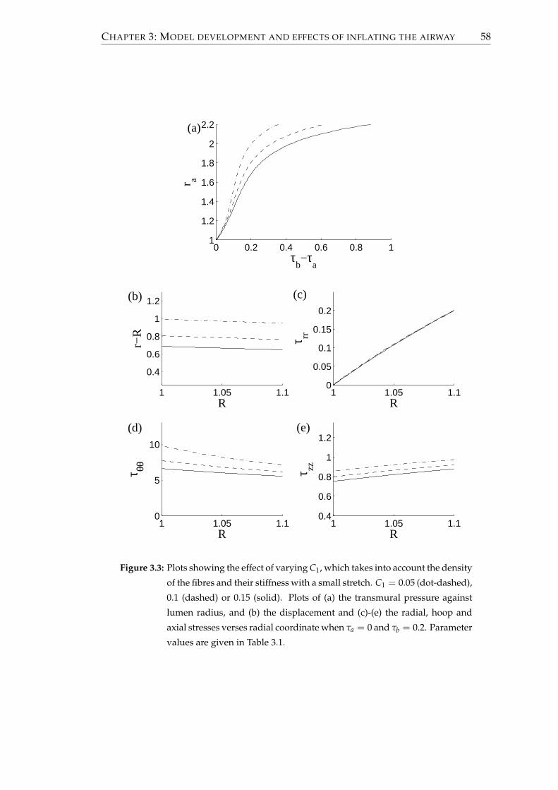
CHAPTER 3: MODEL DEVELOPMENT AND EFFECTS OF INFLATING THE AIRWAY 58
0 0.2 0.4 0.6 0.8 11
1.2
1.4
1.6
1.8
2
2.2
τb−τ
a
r a
(a)
1 1.05 1.1
0.4
0.6
0.8
1
1.2
R
r−R
1 1.05 1.10
0.05
0.1
0.15
0.2
R
τ rr
1 1.05 1.10
5
10
R
τ θθ
1 1.05 1.10.4
0.6
0.8
1
1.2
R
τ zz(b)
(e)(d)
(c)
Figure 3.3: Plots showing the effect of varying C1, which takes into account the density
of the fibres and their stiffness with a small stretch. C1 = 0.05 (dot-dashed),
0.1 (dashed) or 0.15 (solid). Plots of (a) the transmural pressure against
lumen radius, and (b) the displacement and (c)-(e) the radial, hoop and
axial stresses verses radial coordinate when τa = 0 and τb = 0.2. Parameter
values are given in Table 3.1.

CHAPTER 3: MODEL DEVELOPMENT AND EFFECTS OF INFLATING THE AIRWAY 59
of each fibre as it is stretched, is varied. For small transmural pressures, varying C2 has
little effect (a). However, for larger values of the transmural pressure, increasing C2
stiffens the airway wall. Similar to increasing C1, increasing C2 has little effect on the
radial stress distribution (c), while the displacement (b), and the hoop and axial stresses
(d, e) decrease. Physiologically C2 depends on the degree of waviness of the fibres, with
larger values indicating the fibres are less wavy. The amount of waviness could depend
on the level of contraction within the airway when the collagen is deposited.
Results are shown in Fig. 3.5 when ϕ, which is the angle of the fibres from the circum-
ferential direction, is varied. The smaller the angle the larger the component of the
fibres that are in the circumferential direction and the stiffer the airway (a). Increasing
ϕ has little effect on the radial stress distribution (c), while the displacement (b), and
the hoop and axial stresses (d, e) increase. For ϕ = π/6 the axial stress decreases from
the inner to the outer boundary of the wall (e). The angle of the ASM fibres is important
when considering airways at different locations within the lung. It has been found that
the fibre angle is greater in the distal airways than in the large proximal airways [31],
so assuming the collagen fibres are aligned to the ASM fibres, the larger angle within
the small airways indicates that the collagen will produce less resistance to inflation.
Finally, results are shown in Fig. 3.6 when χ, which is the dimensionless undeformed
thickness of the airway wall, is varied. Thickening the wall results in a larger transmu-
ral pressures being required for the same increase in the lumen radius (a). Increasing
χ, the displacement (b), and the hoop and axial stresses (d, e) decrease. The gradient of
the radial stress is reduced in the thickened wall (c). Thickening of the wall is character-
istic of airway wall remodelling in asthmatics [11, 58, 145], with these results showing
that remodelled airways are stiffer, so less easily inflated.
3.2 Airway wall embedded in parenchyma
Having considered the airway wall in isolation, we consider the airway wall embed-
ded in parenchyma. In this section we make the assumption that the parenchyma is
nonlinearly elastic.
3.2.1 Elastic model of the parenchyma
In Sec. 3.1.1 a relationship was found between the pressures exerted on the airway
wall and the lumen radius. Due its compressibility, it is not possible to find a similar
analytical relationship for the parenchyma. An equation can however be found that

CHAPTER 3: MODEL DEVELOPMENT AND EFFECTS OF INFLATING THE AIRWAY 60
0 0.2 0.4 0.61
1.2
1.4
1.6
1.8
2
2.2
τb−τ
a
r a
(a)
1 1.05 1.1
0.4
0.6
0.8
1
1.2
R
r−R
1 1.05 1.10
0.05
0.1
0.15
0.2
R
τ rr
1 1.05 1.10
5
10
R
τ θθ
1 1.05 1.10.4
0.6
0.8
1
1.2
R
τ zz
(d)
(b) (c)
(e)
Figure 3.4: Plots showing the effect of varying C2, which controls the nonlinear in-
crease in stiffness of each fibre as it is stretched. C2 = 0.09 (dot-dashed),
0.14 (dashed) or 0.19 (solid). Plots of (a) the transmural pressure against
lumen radius, and (b) the displacement and (c)-(e) the radial, hoop and ax-
ial stresses verses radial coordinate when τa = 0 and τb = 0.2. Parameter
values are given in Table 3.1.

CHAPTER 3: MODEL DEVELOPMENT AND EFFECTS OF INFLATING THE AIRWAY 61
0 0.1 0.2 0.3 0.4 0.51
1.2
1.4
1.6
1.8
2
2.2
τb−τ
a
r a
(a)
1 1.05 1.1
0.4
0.6
0.8
1
1.2
R
r−R
1 1.05 1.10
0.05
0.1
0.15
0.2
R
τ rr
1 1.05 1.10
5
10
R
τ θθ
1 1.05 1.10.4
0.6
0.8
1
1.2
R
τ zz
(b) (c)
(e)(d)
Figure 3.5: Plots showing the effect of varying ϕ, which is the angle of the fibres from
the circumferential direction. ϕ = 0 (solid), π/12 (dashed) or π/6 (dot-
dashed). Plots of (a) the transmural pressure against lumen radius, and
(b) the displacement and (c)-(e) the radial, hoop and axial stresses verses
radial coordinate when τa = 0 and τb = 0.2. Parameter values are given in
Table 3.1.
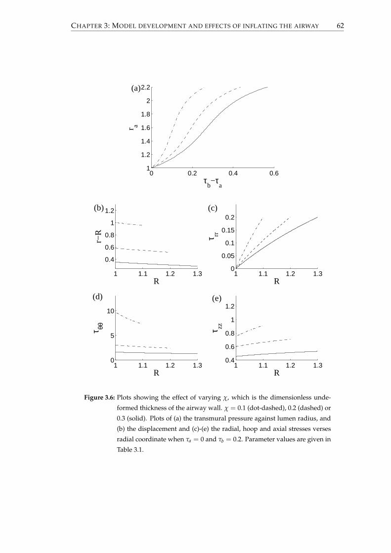
CHAPTER 3: MODEL DEVELOPMENT AND EFFECTS OF INFLATING THE AIRWAY 62
0 0.2 0.4 0.61
1.2
1.4
1.6
1.8
2
2.2
τb−τ
a
r a
(a)
1 1.1 1.2 1.3
0.4
0.6
0.8
1
1.2
R
r−R
1 1.1 1.2 1.30
0.05
0.1
0.15
0.2
R
τ rr
1 1.1 1.2 1.30
5
10
R
τ θθ
1 1.1 1.2 1.30.4
0.6
0.8
1
1.2
R
τ zz
(b) (c)
(d) (e)
Figure 3.6: Plots showing the effect of varying χ, which is the dimensionless unde-
formed thickness of the airway wall. χ = 0.1 (dot-dashed), 0.2 (dashed) or
0.3 (solid). Plots of (a) the transmural pressure against lumen radius, and
(b) the displacement and (c)-(e) the radial, hoop and axial stresses verses
radial coordinate when τa = 0 and τb = 0.2. Parameter values are given in
Table 3.1.

CHAPTER 3: MODEL DEVELOPMENT AND EFFECTS OF INFLATING THE AIRWAY 63
can be solved numerically to find the radius across the parenchyma, which then allows
the stress distributions to be found.
From (2.2.39), the nonzero components of the Cauchy stress tensor are given by
τrr =$
λ(p)
(r′rR− 1
)− R
r′r+
r′Rr
, (3.2.1a)
τθθ =τrr + $
(r
Rr′− r′R
r
), (3.2.1b)
τzz =τrr + $
(Rr′r− r′R
r
). (3.2.1c)
The equation for conservation of momentum is given by (2.2.41) and from (2.2.43) there
are the following boundary conditions:
τrr(Rb) = τb, (3.2.2a)
τrr(Rp) = τp or r(Rp) = rp. (3.2.2b)
Using (3.2.1) in (2.2.41) yields(
r′′rR
+(r′)2
R− r′r
R2
)+
1λ(p)
(r′′R
r+
r′
r− 1
r′r+
Rr′′
(r′)2r+
Rr2 −
1R
)= 0, (3.2.3)
where we have assumed that $ 6= 0. This can be solved numerically with (3.2.1a) and
(3.2.2) to find r and r′ across the layer. Before introducing the numerical methods to do
this, we first show that when the boundary stresses are small our results match those
of Brook et al. [22].
3.2.2 Small deformations
In this section the results for the parenchyma from the previous subsection are lin-
earised, in order to ensure that the model predictions match those of the linear model
of Brook et al. [22]. In the undeformed configuration the parenchyma is stress-free and
r = R, thus we linearise by letting
τ = ετ, r = R + εr, (3.2.4)
where 0 < ε ¿ 1 and τ and r are O(1). Taking the leading order terms, (3.2.1) becomes
τrr = $λ(p)( r
R+ r′ − 2
)+ 2$(r′ − 1), (3.2.5a)
τθθ = τrr + 2$( r
R− r′
), (3.2.5b)
τzz = τrr − 2$(r′ − 1). (3.2.5c)

CHAPTER 3: MODEL DEVELOPMENT AND EFFECTS OF INFLATING THE AIRWAY 64
Using the linearised version of the conservation of momentum equation, (2.2.42), yields
∂τrr
∂R=
2$
R
( rR− r′
), (3.2.6)
hence differentiating (3.2.5a) to find an alternative expression for ∂τrr/∂R,
$(λ(p) + 2)(
r′′ +r′
R− r
R2
)= 0. (3.2.7)
Therefore, the deformed radius is of the form
r = AR +BR
. (3.2.8)
Substituting this into (3.2.5a) and applying the stress boundary conditions from (3.2.2),
the nonzero components of the Cauchy stress tensor satisfy
τrr = τb + (τp − τb)R2
p
R2p − R2
b
R2 − R2b
R2 , (3.2.9a)
τθθ = τb + (τp − τb)R2
p
R2p − R2
b
R2 + R2b
R2 , (3.2.9b)
τzz =
[τb + (τp − τb)
R2p
R2p − R2
b
]λ(p)
λ(p) + 1. (3.2.9c)
The displacement satisfies
r− R = B2(R)τp − B1(R)τb, (3.2.10)
where
B1(R) =R2
b
[R2 + R2
p(λ(p) + 1)]
2$R(R2p − R2
b)(λ(p) + 1), B2(R) =
R2p
[R2 + R2
b(λ(p) + 1)]
2$R(R2p − R2
b)(λ(p) + 1). (3.2.11)
Redimensionalising (3.2.10) yields
r∗ − R∗ =R∗2
p
[R∗2µ(p)∗ + R∗2
b
(λ(p∗) + µ(p)∗
)]
2µ(p)∗R∗(
R∗2p − R∗2
b
) (λ(p)∗ + µ(p)∗)τ∗p
−R∗2
b
[R∗2µ(p)∗ + R∗2
p
(λ(p∗) + µ(p)∗
)]
2µ(p)∗R∗(
R∗2p − R∗2
b
) (λ(p)∗ + µ(p)∗)τ∗b , (3.2.12)
which agrees with the dimensional version of (S.8a) in [22]. Likewise, redimensional-
ising (3.2.9) agrees with the dimensional version of (S.6), for the parenchyma, in [22].

CHAPTER 3: MODEL DEVELOPMENT AND EFFECTS OF INFLATING THE AIRWAY 65
3.2.3 Numerical methods
We now introduce the numerical techniques used to solve (3.2.3) and couple the
parenchyma to the airway wall. First we recall the following boundary conditions
from (2.2.43):
τ(w)rr (1) =τa, (3.2.13a)
r(w)(Rb) =r(p)(Rb) = rb, (3.2.13b)
τ(w)rr (Rb) =τ
(p)rr (Rb) = τb, (3.2.13c)
τ(p)rr (Rp) =τp or r(Rp) = rp. (3.2.13d)
At present the values of rb and τb are unknown. From (3.2.13b) the radius of the
outer boundary of the airway wall is equal to the radius of the inner boundary of the
parenchyma. τb is the value of the radial stress at the outer boundary of the airway
wall and the inner boundary of the parenchyma (3.2.13c). For a given value of rb, us-
ing (3.1.8) yields an estimate for τb in terms of rb and τa, the radial stress at the inner
boundary of wall, which is given by (3.2.13a). In order to ensure that the final boundary
condition (3.2.13d) is satisfied, (3.2.3) must be solved.
Rearranging (3.2.3) yields
r′′ =r′(r− r′R)
(λ(p)(r′)2r2 + r′rR + R2
)
Rr(λ(p)(r′)2r2 + R2(r′)2 + R2), (3.2.14)
which may be rewritten as the following two first order ODEs:
r′ =y, (3.2.15a)
y′ =y(r− yR)
(λ(p)y2r2 + yrR + R2
)
Rr(λ(p)y2r2 + R2y2 + R2). (3.2.15b)
In order to solve (3.2.15) across the parenchyma a shooting algorithm is applied. Se-
lecting initial guesses for rb and r′b, ode45, an ordinary differential equation solver in
MATLAB, is used to shoot from R = Rb to R = Rp. This yields values for r and r′
for a series of points with Rb ≤ R ≤ Rp. Checks are made to see whether, when us-
ing (3.2.1a), τrr(Rb) = τb to satisfy (3.2.13c) and τrr(Rp) = τp or r(Rp) = rp to satisfy
(3.2.13d). In general these conditions will not be satisfied and the estimates of rb and r′bmust be altered. The MATLAB root-finding function fzero is used to alter r′b, so that
the boundary condition (3.2.13c) is met when shooting from R = Rb to R = Rp. In
general (3.2.13d) will still not be satisfied and fzero is again used to update rb. There
are now two new estimates for rb and r′b. The process can be repeated until (3.2.13c)
and (3.2.13d) are satisfied. Once met, the values of r and r′ for a number of points of

CHAPTER 3: MODEL DEVELOPMENT AND EFFECTS OF INFLATING THE AIRWAY 66
R across the parenchyma are known. Inserting these into (3.2.1) gives the stress distri-
butions within the parenchyma. The radius at each point within the airway wall can
be found by using rb and (3.1.3), while (3.1.6) and (3.1.9) can be used to find the stress
distributions. The methods used to select an appropriate accuracy for the MATLAB
ODE solver, used for the shooting, are described in Appendix A.
3.2.4 The choice of parameters
Embedding the airway wall in the parenchyma, values must be selected for the fol-
lowing additional parameters: the compressibility of the parenchyma given by λ(p) =
2ν(p)/(1− 2ν(p)), the ratio of the shear stress of the two layers given by $ and the un-
deformed outer boundary of the parenchyma given by Rp.
A number of experiments have been devised to try to establish properties of the lung
parenchyma, with varying results. The Poisson ratio has been calculated as ν(p) =
0.3 [65] or ν =(p) 0.43 [92]. Unless otherwise stated we shall let ν(p) = 0.3, as used by
Brook et al. [22].
$ = µ(p)∗/µ(w)∗, or in terms of the Young’s modulus of the isotropic component of the
inner and outer layers
$ =3E(p)∗
2(1 + ν(p))E(w)∗ . (3.2.16)
From Brook et al. [22] it is reasonable to set E(w)∗/E(p)∗ = 10, so if ν(p) = 0.3, $ = 3/26.
The thickness of the parenchyma is much greater than that of the airway wall so that
Rp − Rb À χ. Unless otherwise stated, we let Rp = 10.
3.2.5 Comparison to previous work
Before going on to show results for the airway embedded within the parenchyma, our
model predictions are compared to those of Lai-Fook et al. [91]. They carried out an
experiment where they inflated the lung uniformly and then removed a cylindrical
shaped piece of parenchyma. Due to a small reduction in the recoil pressure where the
tissue was removed, there was an increase in the radius of the cylindrical hole. They
used continuum modelling to predict the increase in the radius. Initially they used a
linear model, which predicts that the shear modulus of the parenchyma, but not the
Poisson ratio, affects the findings. The linear model predicts no change in the volume
of the parenchyma. However, due to the size of the displacements, they repeated the
calculations with a nonlinear model. With the revised model they found that there is

CHAPTER 3: MODEL DEVELOPMENT AND EFFECTS OF INFLATING THE AIRWAY 67
1 2 3 4 5 6 7 8 9 101
1.05
1.1
1.15
r
Rel
ativ
e pa
renc
hym
al d
ensi
ty
Figure 3.7: Plots of the parenchymal density relative to the density in the unstressed
state. The internal normal pressure is τa = −1, while τp = 0 and ν = 0.3.
The two curves are for Rp = 10 (solid) and Rp = 100 (dashed).
in fact a small region localised about the cylinder, for which the parenchyma is com-
pressed.
By ignoring the contribution of the airway wall, a stress is applied to the inner bound-
ary of the parenchyma by prescribing τb, while letting τp = 0. The density of the
parenchyma after the deformation, relative to the density prior to the deformation, is
found. This is done by dividing the cross-sectional area of a deformed region by the
cross-sectional area of the region prior to deformation, so that the density
D =(R + ∆R)2 − R2
r(R + ∆R)2 − r(R)2 . (3.2.17)
Results are shown in Fig. 3.7. When Rp = 10 (solid), there is an increase in the
parenchymal density across the parenchyma, although it is increased further near the
inner boundary. One of the assumptions of the model of Lai-Fook et al. [91] though
was that the parenchyma is infinite. If the size of the parenchyma is increased, so that
Rp = 100 (dashed), the relative density is very close to 1 everywhere except near to
the inner boundary, where it is increased. This shows that the majority of the compres-
sion occurs in a small region about the inner boundary, which is in agreement with the
findings of Lai-Fook et al. [91].

CHAPTER 3: MODEL DEVELOPMENT AND EFFECTS OF INFLATING THE AIRWAY 68
Figure τa τp ν(p) E(w)∗/E(p)∗
3.8 * * 0.3 10
3.9 0 0.1, 0.2, 0.3, 0.4 0.3 10
3.10 -0.1, -0.2, -0.3, -0.4 0 0.3 10
3.11 0 0.3 0.2, 0.3, 0.43 10
3.12 -0.3 0 0.2, 0.3, 0.43 10
3.13 0 0.3 0.3 5, 10, 100
3.14 -0.3 0 0.3 5, 10, 100
Table 3.2: The parameter values that vary for the figures listed. For all of the fig-
ures C1 = 0.05, C2 = 0.14, ϕ = π/12, χ = 0.2, Rp = 10. $ =
3E(p)∗/(
2(1 + ν(p))E(w)∗)
. *With Fig. 3.8 a range of values of τa and τp
are used.
3.2.6 Results
In this subsection we show results for the airway embedded within the parenchyma.
We show that the method used to inflate the airway is important. We also show the
effect of altering the Poisson ratio of the parenchyma or the ratio of the shear moduli
of the two layers on these distributions. The parameter values that are used for the
graphs are given in Table 3.2.
We introduce two ways of inflating the airway, which we will refer to as internal and
external inflation and define as follows:
• External inflation - τa = 0 and τp is increased so that the outer boundary is pulled
out,
• Internal inflation - τp = 0 and τa is decreased so that the inner boundary is pushed
out.
Physiologically, external and internal inflation correspond to normal breathing and ar-
tificial ventilation, respectively. Plots of the lumen radius against the transpulmonary
pressure are shown in Fig. 3.8. Larger transpulmonary pressures are required for the
same increase in the lumen radius when inflating the airway externally (dashed) than
when inflating internally (solid). In both cases the fibres within the airway wall ensure
that as the airway inflates, it stiffens. These results show that smaller pressure differ-
ences are required to inflate the airways with artificial ventilation than with normal
breathing.
Plots are shown in Fig. 3.9 of the distribution of the radial displacement and the

CHAPTER 3: MODEL DEVELOPMENT AND EFFECTS OF INFLATING THE AIRWAY 69
0 0.1 0.2 0.3 0.4 0.5 0.61
1.5
2
2.5
τp−τ
a
r a
Figure 3.8: Curves of the lumen radius against the transpulmonary pressure, when the
airway is inflated externally (dashed, τa = 0) or internally (solid, τp = 0).
Parameter values are given in Table 3.2.
stresses across the airway for various values of the transpulmonary pressure, when
the airway is inflated externally (corresponding to normal breathing). Considering the
radial displacement, there are large displacements within the parenchyma (a). One
method for ensuring that the displacement within the parenchyma is not unrealisti-
cally large, would be to use the alternate boundary condition for the outer boundary
of the parenchyma, (3.2.2b), and prescribe rp rather than τp. The stresses in the radial,
hoop and axial directions are positive throughout indicating that the tissue is under
tension (b-d). The radial stress varies a lot across the airway wall, whereas there is
little variation within the parenchyma (b). The hoop and axial stresses are discon-
tinuous at the boundary between the two layers (c, d). When modelling arteries as
multi-layered structures, Holzapfel et al. [61] found similar discontinuities in the hoop
and axial stresses at the boundaries between the layers. Also similar to their findings
are that the magnitude of the hoop and axial stresses are much larger than those of the
radial stresses, at least in the airway wall. Within the airway wall the hoop stress is
greatest at the inner boundary (c), while the axial stress is greatest at the outer bound-
ary (d).
Secondly for the case that the airway is inflated internally (mimicking artificial ven-
tilation), the radial displacement and the stress distributions are shown in Fig. 3.10.
The displacement is greatest at the inner boundary, with the airway wall shielding the
parenchyma from large displacements (a). The radial stress is negative, indicating that
the tissue is under tension in the radial direction (b). There is more variation in the ra-
dial stress within the airway wall than in the parenchyma. The hoop stress is similar to

CHAPTER 3: MODEL DEVELOPMENT AND EFFECTS OF INFLATING THE AIRWAY 70
100
101
0
2
4
6
8
R
r−R
100
101
0
0.1
0.2
0.3
0.4
R
τrr
100
101
0
5
10
15
R
τθθ
100
101
0
0.5
1
1.5
R
τzz
(d)
(b)(a)
(c)
Figure 3.9: Curves showing the (a) displacement and (b)-(d) the radial, hoop and axial
stresses verses radial coordinate for a two-layer annulus with τa = 0 and
τp = 0.1 (dashed), τp = 0.2 (dotted), τp = 0.3 (dot-dashed) and τp = 0.4
(solid). Parameter values are given in Table 3.2.

CHAPTER 3: MODEL DEVELOPMENT AND EFFECTS OF INFLATING THE AIRWAY 71
100
101
0
0.2
0.4
0.6
0.8
1
R
r−R
100
101
−0.4
−0.3
−0.2
−0.1
0
R
τrr
100
101
0
2
4
6
8
R
τθθ
100
101
0
0.1
0.2
0.3
0.4
0.5
0.6
R
τzz
(c)
(a) (b)
(d)
Figure 3.10: Curves showing the (a) displacement and (b)-(d) the radial, hoop and
axial stresses verses radial coordinate for a two-layer annulus with τp = 0
and τa = −0.1 (dashed), τa = −0.2 (dotted), τa = −0.3 (dot-dashed) and
τa = −0.4 (solid). Parameter values are given in Table 3.2.
when the airway is inflated externally. Positive stresses indicate that the tissue is under
compression in the circumferential direction (c), with a discontinuity at the boundary
between the two layers and greatest stress at the inner boundary of the airway wall.
Within the airway wall the axial stress is similar to when the airway is inflated ex-
ternally, with positive stresses that are greatest at the outer boundary of the wall (d).
Within the parenchyma the axial stress is very small, with compressive stresses close to
the airway wall, while further away there are tensile stresses.
In Sec. 3.2.4 we noted that different values had been calculated experimentally for the
Poisson ratio of the parenchyma. We therefore investigate what effect varying ν(p) has
on the results. In Fig. 3.11 results are shown when the airway is inflated externally,
with ν(p) = 0.2, ν(p) = 0.3 (as found in [65]) or ν(p) = 0.43 (as found in [92]). Increasing

CHAPTER 3: MODEL DEVELOPMENT AND EFFECTS OF INFLATING THE AIRWAY 72
ν(p), increases the transpulmonary pressure that is required for same increase in the
lumen radius (a). For larger values of ν(p), there is reduced radial displacement, and
stress across the two layers (b, c), while the hoop and axial stresses are reduced within
the airway wall, but increased within the parenchyma (d, e). With ν(p) = 0.2 the radial
stress peaks at the boundary of the two layers. Therefore, smaller displacements result
if the parenchyma is less compressible. These differences are most noticeable within
the parenchyma.
The effect of changing the Poisson ratio when inflating the airway internally are shown
in Fig. 3.12. There is less variation between the curves for the different levels of
parenchymal compressibility than when the airway was inflated externally. The airway
is again stiffer with larger values of ν(p) (a). Larger values of ν(p) also result in reduced
displacement, except for the outer region of the parenchyma where there is an increase
in the displacement (b). The radial stress (c) and the hoop and axial stresses within
the airway wall (d, e) are smaller for larger values of ν(p). Within the parenchyma, the
hoop stress is increased slightly with increased ν(p), while the axial stress is increased
slightly in the inner part of the parenchyma, but decreased slightly in the outer part
of the parenchyma. Similar to with external inflation, although to a smaller extent, the
airway is inflated less if the parenchyma is less compressible.
We have considered a fixed value of the ratio of the shear modulus of the parenchyma
to the base matrix of the airway wall. However, there is evidence that the shear modu-
lus of the parenchyma is linearly related to the transpulmonary pressure [160], so that
as the transpulmonary pressure increases, $ also increases. In the next two figures we
consider the effect of altering $. Firstly, the effect of altering $ when the airway is in-
flated externally is shown in Fig. 3.13. For smaller values of $, when the stiffness of the
airway wall is closer to that of the parenchyma, larger transpulmonary pressures, rela-
tive to the shear modulus of the wall matrix, are required for the same increase in the
lumen radius (a). The distribution of the radial displacement and stress and the hoop
and axial stresses are increased as $ is increased (b-e), except for the hoop stress within
the parenchyma, where it has a decreased value (d). In particular, the shape of the ra-
dial stress distribution is altered, so that while τb < τp for the curves drawn using the
smaller two values of $, τrr peaks at the boundary for the largest value. These results
therefore show that increased values of the shear modulus of the parenchyma, and
thus of $, as may be appropriate for high transpulmonary pressures, lead to a stiffer
airway and reduced inflation. The problem of large displacements predicted within
the parenchyma is also reduced.
Similar alterations are seen when $, the ratio of the shear stress of the two layers, is

CHAPTER 3: MODEL DEVELOPMENT AND EFFECTS OF INFLATING THE AIRWAY 73
0 0.1 0.2 0.3 0.4 0.5 0.6 0.71
1.5
2
2.5
τp−τ
a
r a
(a)
100
101
0
2
4
6
8
10
R
r−R
100
101
0
0.1
0.2
0.3
0.4
R
τrr
100
101
0
2
4
6
8
10
R
τθθ
100
101
0.2
0.4
0.6
0.8
1
1.2
R
τzz
(e)
(c)(b)
(d)
Figure 3.11: Plots showing the effect of ν(p), the Poisson ratio of the parenchyma,
when inflating the airway externally. ν = 0.2 (dashed), 0.3 (solid) and 0.43
(dot-dashed). Plots of (a) the lumen radius against the transpulmonary
pressure, and distributions of (b) the displacement and (c)-(e) the radial,
hoop and axial stresses verses radial coordinate. Parameter values are
given in Table 3.2.
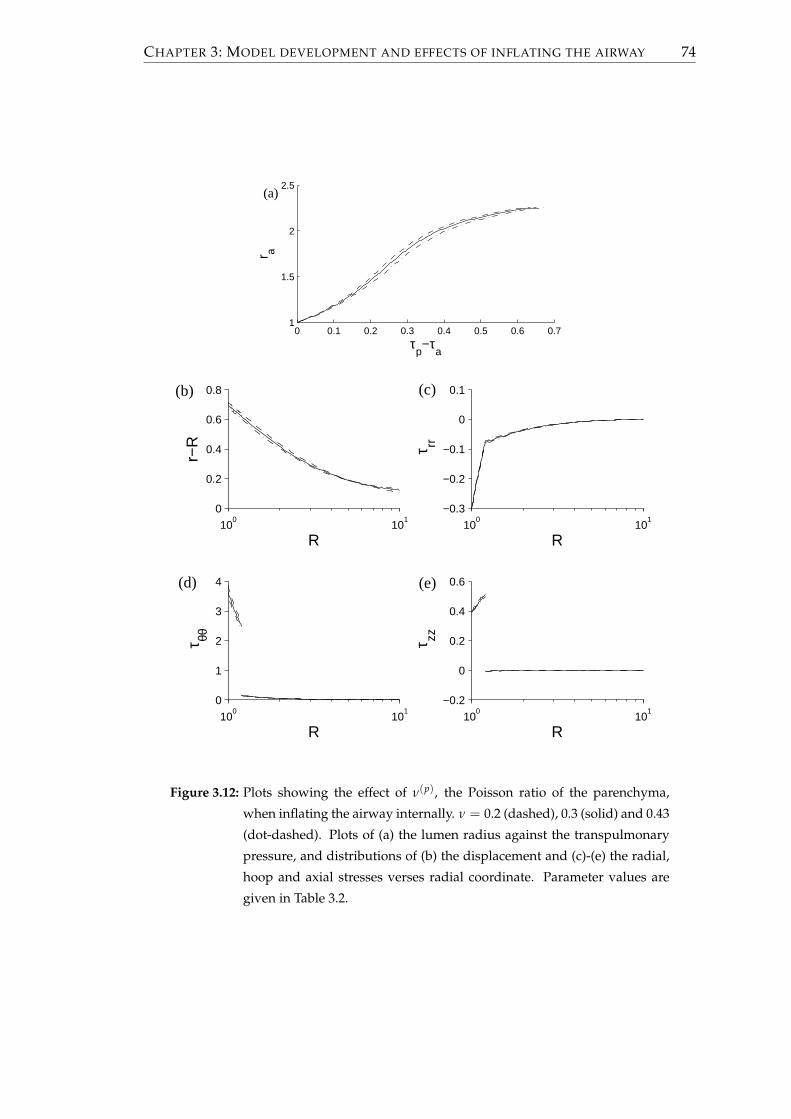
CHAPTER 3: MODEL DEVELOPMENT AND EFFECTS OF INFLATING THE AIRWAY 74
0 0.1 0.2 0.3 0.4 0.5 0.6 0.71
1.5
2
2.5
τp−τ
a
r a
(a)
100
101
0
0.2
0.4
0.6
0.8
R
r−R
100
101
−0.3
−0.2
−0.1
0
0.1
R
τrr
100
101
0
1
2
3
4
R
τθθ
100
101
−0.2
0
0.2
0.4
0.6
R
τzz
(d) (e)
(c)(b)
Figure 3.12: Plots showing the effect of ν(p), the Poisson ratio of the parenchyma,
when inflating the airway internally. ν = 0.2 (dashed), 0.3 (solid) and 0.43
(dot-dashed). Plots of (a) the lumen radius against the transpulmonary
pressure, and distributions of (b) the displacement and (c)-(e) the radial,
hoop and axial stresses verses radial coordinate. Parameter values are
given in Table 3.2.

CHAPTER 3: MODEL DEVELOPMENT AND EFFECTS OF INFLATING THE AIRWAY 75
0 0.1 0.2 0.3 0.4 0.5 0.6 0.7 0.81
1.5
2
2.5
τp−τ
a
r a
(a)
100
101
0
10
20
30
R
r−R
100
101
0
0.1
0.2
0.3
0.4
R
τrr
100
101
0
5
10
R
τθθ
100
101
0
0.5
1
R
τzz
(c)
(e)(d)
(b)
Figure 3.13: Plots showing the effect of $, the ratio of the shear stress of the two layers,
when inflating the airway externally. $ = 3/13 (dashed), 3/26 (solid) and
3/260 (dot-dashed). Plots of (a) the lumen radius against the transpul-
monary pressure, and (b) the displacement and (c)-(e) the radial, hoop
and axial stresses verses radial coordinate. Parameter values are given in
Table 3.2.
CHAPTER 3: MODEL DEVELOPMENT AND EFFECTS OF INFLATING THE AIRWAY 76
altered and the airway is inflated internally, with a couple of exceptions (Fig. 3.14). The
radial stress no longer peaks at the boundary between the two layers when $ = 3/260
(c, dot-dashed) and within the outer section of the parenchyma, the axial stress is now
reduced for larger values of $ (e). These results therefore also show that increased
values of the shear modulus of the parenchyma, and thus of $, lead to a stiffer airway
and reduced inflation when the airway is internally inflated.
3.3 Viscoelastic behaviour of airway wall embedded in
parenchyma
In this section we again consider the airway wall embedded in parenchyma, but now
assume that the parenchyma is linearly viscoelastic.
3.3.1 Viscoelastic model of the parenchyma
The nonzero components of the Cauchy stress tensor are given in (2.2.40). Assuming
that times are nondimensionalised with respect T∗ = t∗r , from (2.2.42),[
∂
∂t+ 1
]∂τrr
∂R+
τrr − τθθ
R= $
(λ(p) + 2
) [tc
∂
∂t+ 1
] (r′′ +
r′
R− r
R2
)= 0. (3.3.1)
This may be rewritten in the form
∂
∂t
exp
(ttc
) (r′′ +
r′
R− r
R2
)= 0, (3.3.2)
which, integrating and assuming that initially the airway is in the stress-free unde-
formed steady state, yields
r′′ +r′
R− r
R2 = 0, (3.3.3)
so like in Sec. 3.2.2 the deformed radius is of the form
r = AR +BR
. (3.3.4)
Substituting into (2.2.40) and applying the boundary conditions (3.2.2a) and the stress
option from (3.2.2b), yields
τrr(R, t) = τb(t) + (τp(t)− τb(t))R2
p
R2p − R2
b
R2 − R2b
R2 , (3.3.5a)
τθθ(R, t) = τb(t) + (τp(t)− τb(t))R2
p
R2p − R2
b
R2 + R2b
R2 , (3.3.5b)
τzz(R, t) =
[τb(t) + (τp(t)− τb(t))
R2p
R2p − R2
b
]λ(p)
λ(p) + 1(3.3.5c)

CHAPTER 3: MODEL DEVELOPMENT AND EFFECTS OF INFLATING THE AIRWAY 77
0 0.2 0.4 0.6 0.8 11
1.5
2
2.5
τp−τ
a
r a
(a)
100
101
0
0.5
1
R
r−R
100
101
−0.25
−0.2
−0.15
−0.1
−0.05
R
τrr
100
101
0
2
4
6
8
R
τθθ
100
101
0
0.2
0.4
0.6
R
τzz
(e)(d)
(c)(b)
Figure 3.14: Plots showing the effect of $ when inflating the airway internally. $ =
3/13 (dashed), 3/26 (solid) and 3/260 (dot-dashed). Plots of (a) the lu-
men radius against the transpulmonary pressure, and (b) the displace-
ment and (c)-(e) the radial, hoop and axial stresses verses radial coordi-
nate. Parameter values are given in Table 3.2.
CHAPTER 3: MODEL DEVELOPMENT AND EFFECTS OF INFLATING THE AIRWAY 78
with the displacements satisfying[
tc∂
∂t+ 1
](r(R, t)− R) =
[∂
∂t+ 1
] [B2(R)τp(t)− B1(R)τb(t)
], (3.3.6)
where B1(R) and B2(R) are given in (3.2.11). Alternatively (3.3.5) and (3.3.6) may be
obtained by applying the nondimensional version of (1.5.51),
τ → dτ
dt+ τ, r → tc
drdt
+ r, (3.3.7)
to the linear equations (3.2.9) and (3.2.10). While stresses within the parenchyma re-
spond instantaneously to any changes in the τb and τp, displacements do not.
Integrating (3.3.6) and assuming that initially the airway is in the stress-free unde-
formed steady state yields
r(R, t)− R = B2(R)I2(t)− B1(R)I1(t), (3.3.8)
where
I1(t) = exp(− t
tc
) ∫ t
s=0exp
(stc
) [dds
+ 1]
τb(s)tc
ds, (3.3.9a)
I2(t) = exp(− t
tc
) ∫ t
s=0exp
(stc
) [dds
+ 1]
τp(s)tc
ds. (3.3.9b)
In order to solve (3.3.8) or (3.3.13), to find the displacement, it is necessary to first find
τb(t), the radial stress at the boundary. At present rb, the radius of the boundary, is not
known. Considering (3.3.6) at R = Rb and using (3.1.8) to get an expression for τb in
terms of rb, if τp is prescribed,
F1drb
dt=
[ddt
+ 1]
B2(Rb)τp − B1(Rb)(
τa + 2 cos2 ϕ∫ Rb
1
AR
dR)
− (rb − Rb)
− B1(Rb)
log
(raRb
rb
)+
(r2b − R2
b)(R2b − 1)
2r2ar2
b+ H(rb − Rb)C1
√π
C2cos2 ϕ
(erfi
√C2
(r2
b − R2b)
cos2 ϕ− erfi
√C2
(r2
b − R2b
R2b
)cos2 ϕ
) , (3.3.10)
where ra =√
r2b − R2
b + 1 and
F1 =tc + B1(Rb)
((R2
b − 1)(R2br2
a + r2b)
r4ar3
b+ H(rb − Rb)4C1 cos4 ϕrb
exp
[C2(rb − Rb)4 cos4 ϕ
]− 1
Rbexp
[C2(rb − Rb)4 cos4 ϕ
R4b
] ). (3.3.11)
τa and τp are given by the boundary conditions and A is assumed to be known, with
A = 0 in this chapter.

CHAPTER 3: MODEL DEVELOPMENT AND EFFECTS OF INFLATING THE AIRWAY 79
Equations (3.3.5) to (3.3.11) are suitable when τp is prescribed. Alternatively if rp is
prescribed, by letting R = Rp in (3.3.8) yields[
tc∂
∂t+ 1
](r(R, t)− R) =
[∂
∂t+ 1
] [B2(R)B1(Rp)
B2(Rp)− B1(R)
]τb(t)
+B2(R)B2(Rp)
[tc
∂
∂t+ 1
](rp − Rp). (3.3.12)
Integrating gives the displacement within the parenchyma as follows:
r(R, t)− R =B2(R)B2(Rp)
(rp − Rp
)+
[B2(R)B2(Rp)
B1(Rp)− B1(R)]
I1(t). (3.3.13)
Now drb/dt satisfies
F2drb
dt=
B2(Rb)B2(Rp)
[tc
ddt
+ 1] (
rp − Rp)+
[ddt
+ 1] [
B2(Rb)B1(Rp)B2(Rp)
− B1(Rb)]
(τa + 2 cos2 ϕ
∫ Rb
1
AR
dR)
− (rb − Rb) +[
B2(Rb)B1(Rp)B2(Rp)
− B1(Rb)]
log
(raRb
rb
)+
(r2b − R2
b)(R2b − 1)
2r2ar2
b+ H(rb − Rb)C1
√π
C2cos2 ϕ
(erfi
√C2
(r2
b − R2b)
cos2 ϕ− erfi
√C2
(r2
b − R2b
R2b
)cos2 ϕ
) , (3.3.14)
where
F2 =tc −[
B2(Rb)B1(Rp)B2(Rp)
− B1(Rb)] (
(R2b − 1)(R2
br2a + r2
b)r4
ar3b
+ H(rb − Rb)4C1 cos4 ϕrb
exp
[C2(rb − Rb)4 cos4 ϕ
]− 1
Rbexp
[C2(rb − Rb)4 cos4 ϕ
R4b
] ). (3.3.15)
In order to solve (3.3.10) or (3.3.14), we introduce the following methods of inflating
the airway:
1. τp is linearly increased until τp = τp and then held constant so that
τa(t) = 0, ∀t, τp(t) =
0, if t < 0,
τptti
, if 0 ≤ t ≤ ti,
τp, if t > ti;
(3.3.16)
2. τa is linearly decreased until τa = τa and then held constant so that
τa(t) =
0, if t < 0,
τatti
, if 0 ≤ t ≤ ti,
τa, if t > ti,
τp(t) = 0, ∀t; (3.3.17)

CHAPTER 3: MODEL DEVELOPMENT AND EFFECTS OF INFLATING THE AIRWAY 80
3. An oscillatory force is applied to the outer boundary so that
τa(t) = 0 τp(t) = τp(1− cos(ωt)), t ≥ 0, (3.3.18)
where ω is the dimensionless angular frequency and τp is the amplitude of the
oscillations;
4. The position of the outer boundary is oscillated so that
τa(t) = 0 rp(t) = Rp + rp(1− cos(ωt)), t ≥ 0, (3.3.19)
where ω is the dimensionless angular frequency and rp is the amplitude of the
oscillations.
Using ode45 in MATLAB with the initial condition that rb(0) = Rb we are able to solve
to find rb(t). The displacements within the airway wall can then be found using (3.1.3),
while the stresses can be found using (3.1.6) and (3.1.9). In order to find the displace-
ments within the parenchyma, we first use (3.3.8) at R = Rb to find the following
expression for I1, which may then be inserted into (3.3.8):
I1(t) =rb(t)− Rb − B2(Rb)I2(t)
B1(Rb). (3.3.20)
If rp is prescribed, using (3.3.13) at R = Rb there is the following expression for I1,
which may then be inserted into (3.3.13):
I1(t) =B2(Rp) (rb(t)− Rb)− B2(Rb)
(rp(t)− Rp
)
B2(Rb)B1(Rp)− B1(Rb)B2(Rp). (3.3.21)
All that is left to find is the stresses within the parenchyma. If τp is prescribed, τb is
given by (3.1.8) and the stresses are found using (2.2.40). If rp is prescribed, (3.1.8) is
first differentiated to find an expression for dτb/dt. Using (3.3.12), (3.3.5) is altered to

CHAPTER 3: MODEL DEVELOPMENT AND EFFECTS OF INFLATING THE AIRWAY 81
C1 C2 ϕ χ Rp ν(p) $ µ(w)∗ tc ω
0.05 0.14 π/12 0.2 10 0.3 3/26 20 cm water 4 2π/5
Table 3.3: The parameter values that are used in Sec. 3.3 unless otherwise stated.
give the following equations, which may be updated to find the parenchymal stresses:[
∂
∂t+ 1
]τrr(R, t) =
[ddt
+ 1]
τb(t) +
[tc
ddt
+ 1]
rp − Rp
B2(Rp)+
[ddt
+ 1]
τb
(B1(Rp)B2(Rp)
− 1)
R2p
R2p − R2
b
R2 − R2b
R2 , (3.3.22a)
[∂
∂t+ 1
]τθθ(R, t) =
[ddt
+ 1]
τb(t) +
[tc
ddt
+ 1]
rp − Rp
B2(Rp)+
[ddt
+ 1]
τb
(B1(Rp)B2(Rp)
− 1)
R2p
R2p − R2
b
R2 + R2b
R2 , (3.3.22b)
[∂
∂t+ 1
]τzz(R, t) =
[ [ddt
+ 1]
τb(t) +
[tc
ddt
+ 1]
rp − Rp
B2(Rp)+
[ddt
+ 1]
τb
(B1(Rp)B2(Rp)
− 1)
R2p
R2p − R2
b
]λ(p)
λ(p) + 1. (3.3.22c)
3.3.2 The choice of parameters
A value must be assigned to the parameter tc, which describes the ratio of the creep
timescale to the relaxation timescale. If methods 3 or 4 are used to inflate the airway, a
value must also be chosen for ω. During normal breathing, it is reasonable to assume
that the period of a breath is 5s. While from [135], we expect the stress relaxation time
to be approximately one second. It is therefore appropriate to set ω = 2π/5. The other
parameter values are given in Table 3.3 and are as described previously.
Pressure-volume curves have been produced experimentally for the lung, by incre-
mentally increasing the pressure applied around the lung and measuring the resulting
lung volume. In Fig. 3.15, comparisons are made between the equilibrium loop formed
when using (3.3.18) (left) and a representative pressure-volume curve (right). In order
to take into account the increased period of the oscillation, due to stopping at inter-
mediate pressures, we decrease the angular frequency, so that ω = 2π/20. We set
τp = 0.75 to match the range of transpulmonary pressures applied to the lung. This
allows us to produce a prediction of the cross-sectional area of an airway for given
transpulmonary pressures. For tc = 4, assuming that the airway is of constant length,
there is reasonable agreement between the model predictions and the representative

CHAPTER 3: MODEL DEVELOPMENT AND EFFECTS OF INFLATING THE AIRWAY 82
0 0.5 1 1.50
5
10
15
20
(τp*−τ
a*)/µ(m)*
π r a2
0 10 20 300
0.5
1
Pressure around lung (cmH20)
Vol
ume
(L)
Figure 3.15: Left: Equilibrium loop of the cross-sectional area of an airway against the
transpulmonary pressure from (3.3.18), when tc = 4, τp = 0.75 and ω =
2π/20. The other parameter values are given in Table 3.3. Right: Rep-
resentative picture of a pressure-volume curve for the lung (Data taken
from http://www.studydroid.com/imageCards/0c/fq/card-13101355-
back.jpg).
pressure-volume curve.
Since the choice of tc is based on experiments on the lung as a whole and not just an
airway, the effect, on the relationship between pressure and area, of varying tc is shown
in Fig. 3.16. Increasing the size of tc, increases the amount of hysteresis, with greater
energy loses in each cycle. The airway area, at the point of zero pressure, also increases
as tc increases, resulting in a smaller range of lumen areas over the cycle. The shape of
the curves also become more elliptical.
3.3.3 Results
In this subsection the different methods of inflating the airway described in (3.3.16-
3.3.19) are investigated. Results are shown in Fig. 3.17 for method 1, where the airway
is inflated externally. Initially as τp increases linearly, the radial displacement (a) and
the stresses in the radial (b), hoop (c) and axial (e) directions increase (dot-dashed lines).
The distributions are similar to those observed in Fig. 3.9, where the parenchyma was
elastic. In contrast to the elastic parenchyma though, time is now important, with the
displacement and stress distributions continuing to change once the boundary stresses
are held steady (dashed lines). The radial displacement and stress (a, b) continue to
increase, as do the hoop and axial stresses within the airway wall (d, f). However,
within the parenchyma the hoop and axial stresses reduce slightly. At large time, the
distributions tend towards those found if the parenchyma is modelled using linear

CHAPTER 3: MODEL DEVELOPMENT AND EFFECTS OF INFLATING THE AIRWAY 83
0 0.5 1 1.50
5
10
15
20
τp−τ
a
π r a2
0 0.5 1 1.50
5
10
15
20
τp−τ
a
π r a2
0 0.5 1 1.50
5
10
15
20
τp−τ
a
π r a2
0 0.5 1 1.50
5
10
15
20
τp−τ
a
π r a2
(b)(a)
(c) (d)
Figure 3.16: Plots of the cross-sectional area of an airway against the transpul-
monary pressure from (3.3.18), when the ratio of the creep and relaxation
timescales tc = 2 (a), tc = 4 (b), tc = 6 (c) or tc = 8 (d). τp = 0.75,
ω = 2π/20. The other parameter values are given in Table 3.3.

CHAPTER 3: MODEL DEVELOPMENT AND EFFECTS OF INFLATING THE AIRWAY 84
elasticity (solid line). These results provide evidence that the model is able to predict
the viscoelastic phenomena of creep that has been observed in experiments.
Comparisons are made in Fig. 3.18 between the large-time steady state solution
when the parenchyma is linear or nonlinear and the airway is inflated externally.
This is achieved by making comparisons between models for the airway when the
parenchyma is modelled using linear elasticity (Sec. 3.2.2) or nonlinear elasticity
(Sec. 3.2.1). The linear predictions are shown with solid lines, while the nonlinear pre-
dictions are shown by dashed lines. There is little difference between the two sets
of curves. In each case the distribution of the displacement and the stress is slightly
greater in the nonlinear case, except for the hoop stress within the parenchyma (c),
where it is slightly smaller. The simplification of the linear viscoelastic model over the
nonlinear viscoelastic model appears to give sufficiently good results for this case.
Results are shown in Fig. 3.19 for method 2, where the airway is inflated internally. Ini-
tially as τa decreases linearly, the radial displacement (a) and the stresses in the hoop
and axial directions (d, f) increase (dot-dashed lines). The stress in the radial direction
decreases, indicating that the airway experiences increased compressive forces in this
direction (b). The distributions are similar to those observed in Fig. 3.10, where the
parenchyma was elastic. In contrast to the elastic parenchyma, time is again important,
with the displacement and stress distributions continuing to change once the bound-
ary stresses are held steady (dashed lines). The radial displacement and stress (a, c)
both increase, thus the size of the compressive stresses in the radial direction decrease.
The changes to the hoop and axial (e, g) stresses are different within the airway wall
and within the parenchyma. Within the airway wall the stresses continue to increase,
indicating increased tensile stress, while within the parenchyma the stresses decrease,
indicating decreased tensile stress. At large time, the distributions tend towards those
found if the parenchyma is modelled using linear elasticity (solid line). These results
provide further evidence of the models ability to predict creep.
Comparisons are made in Fig. 3.20 between the large-time steady state solution when
the parenchyma is linear or nonlinear and the airway is inflated internally. There are
greater differences between the two models than when the airway was inflated exter-
nally (Fig. 3.18), although they are still quite small. The displacement and the stresses
are generally a bit larger for the nonlinear case (dashed) compared to the linear case
(solid). Within the outer part of the parenchyma, the radial stress is slightly smaller
with the nonlinear case (b). Within the parenchyma, the axial stress is independent
of R with the linear model (c.f. (3.2.9c)), while this is not the case with the nonlinear
model (c.f. (3.2.9c)), which predicts a smaller value near the inner boundary of the

CHAPTER 3: MODEL DEVELOPMENT AND EFFECTS OF INFLATING THE AIRWAY 85
100
101
0
5
10
R
r−R
100
101
0
0.5
R
τ rr
100
101
0
5
10
R
τ θθ
100
101
0
10
20
R
τ θθ
100
101
0
0.5
1
R
τ zz
100
101
0
1
2
R
τ zz
(a)
(f)(e)
(c) (d)
(b)
Figure 3.17: Plots of (a) the radial displacement and the (b) radial, (c, d) hoop and
(e, f) axial stresses verses radial coordinate, when the airway is inflated
externally using (3.3.16). τp = 0.4 and ti = 1. The dashed lines at plotted
at intervals of ∆t=0.2, while τp is linearly increasing, the dotted lines are
plotted thereafter at intervals of ∆t=1, while τp is held constant, and the
solid line is the corresponding elastic solution. Arrows indicate increasing
time. The other parameter values are given in Table 3.3.

CHAPTER 3: MODEL DEVELOPMENT AND EFFECTS OF INFLATING THE AIRWAY 86
100
101
0
2
4
6
R
r−R
100
101
0
0.2
0.4
R
τ rr
100
101
0
5
10
R
τ θθ
100
101
0
0.5
1
R
τ zz
(c)
(a) (b)
(d)
Figure 3.18: Comparison of the large-time equilibrium solution when the parenchyma
is linearly viscoelastic (solid) or nonlinearly viscoelastic (dashed) when
the airway is inflated externally so that τp = 0.4 and τa = 0. The other
parameter values are given in Table 3.3.

CHAPTER 3: MODEL DEVELOPMENT AND EFFECTS OF INFLATING THE AIRWAY 87
100
101
0
0.2
0.4
0.6
0.8
Rr−
R
(a)
100
101
−0.4
−0.2
0
R
τ rr
100
101
−0.4
−0.2
0
R
τ rr
100
101
0
1
2
R
τ θθ
100
101
0
5
R
τ θθ
100
101
0
0.1
0.2
R
τ zz
100
101
0
0.5
R
τ zz
(g)
(e)
(c)(b)
(d)
(f)
Figure 3.19: Plots of (a) the radial displacement and the (b) radial, (c, d) hoop and
(e, f) axial stresses verses radial coordinate when the airway is inflated
internally using (3.3.17). τa = −0.4 and ti = 1. The dashed lines at
plotted at intervals of ∆t=0.2, while τa is linearly decreasing, the dotted
lines are plotted thereafter at intervals of ∆t=1, while τa is held constant,
and the solid line is the corresponding elastic solution. Arrows indicate
increasing time. The other parameter values are given in Table 3.3.

CHAPTER 3: MODEL DEVELOPMENT AND EFFECTS OF INFLATING THE AIRWAY 88
100
101
0
0.5
1
R
r−R
100
101
−0.4
−0.2
0
R
τ rr
100
101
0
2
4
6
8
R
τ θθ
100
101
0
0.2
0.4
0.6
R
τ zz
(a) (b)
(c) (d)
Figure 3.20: Comparison of the large-time equilibrium solution when the parenchyma
is linearly viscoelastic (solid) or nonlinearly viscoelastic (dashed) when
the airway is inflated internally so that −τa = 0.4 and τp = 0. The other
parameter values are given in Table 3.3.
parenchyma and a larger value near the outer boundary of the parenchyma (d). For a
small section near the inner boundary of the parenchyma, the nonlinear model predicts
a negative value for the axial stress, indicating compressive stresses, which the linear
model is unable to show.
Methods 3 and 4, which have oscillatory boundary conditions, are now considered.
There are differences if the outer radial stress is oscillated (3.3.18) to if the outer radial
displacement is oscillated (3.3.19). Plots of the development of the radial stress, the
displacement at the outer boundary of the parenchyma and at the lumen boundary are
shown in Fig. 3.21. When τp is prescribed, as shown in (a), over the first few oscillations
rp − Rp increases on average (c), before tending to a limit cycle, such that the outer
boundary of the parenchyma does not return to its undeformed position. Similarly,
the displacement at the lumen boundary increases on average (e), so that when a limit
cycle is reached, at all points within the cycle the radius of the lumen is greater than

CHAPTER 3: MODEL DEVELOPMENT AND EFFECTS OF INFLATING THE AIRWAY 89
in the undeformed state. If instead rp is prescribed, so the displacement at the outer
boundary of the parenchyma is as in (d), within the first oscillation τp initially increases
before decreasing and becoming negative (b). When a limit cycle is reached there is
part of each oscillation where τp is positive, indicating tensile stresses and part that is
negative, indicating compressive stresses. At the end of each cycle the displacement of
the lumen radius is negative (f), indicating airway narrowing. With this method, the
parenchyma initially expands and then as its boundary is brought in, the parenchyma
does not contract fully back to its previous configuration, so that the lumen narrows.
It can also be shown that if the airway were to start from some pre-stressed starting
position, so that rp > Rp, the airway would become narrower than it started at. In
reality breathing is probably a combination of the two methods, at least in normal tidal
breathing, with the ribcage lifting to prescribe a displacement, but then the airway
deflating due to lung recoil rather than a prescribed displacement. This may stop the
reduction in the airway lumen being seen as in (b). The reduction of the airway lumen
would also be less of an issue if the airway was initially pre-stressed, and thus slightly
inflated.
The plots in Fig. 3.21 showed that following some initial transient behaviour, limit
cycles were approached. These cycles for the case that τp is prescribed are shown
in Fig. 3.22. There is now evidence of hysteresis, due to the viscoelasticity of the
parenchyma. There are differences between when the airway is inflated to when it
deflates. The displacement is larger as the airway deflates than when inflating (a). The
loop at the edge of the parenchyma is also fatter, indicating that there are larger en-
ergy losses here. At the boundary between the two layers, the radial stress is greater
during deflation than during inflation (b). Within the airway wall the hoop stress (c)
and axial stress (d) are also greater during deflation than inflation. However, within
the parenchyma, the hoop and axial stresses are smaller during deflation than during
inflation.
3.4 Conclusions
In this chapter we have simplified the equations presented in Chapter 2 for an asth-
matic airway. In particular, we concentrated on the dimensionless governing equations
for the tissue-level mechanics (Sec. 2.2.6) and in solving them we assumed that passive
stresses or displacements were applied to the boundaries of the airway, but that there
was no active contractile forcing. These solutions are therefore concerned with the air-
ways when the ASM has not been activated.

CHAPTER 3: MODEL DEVELOPMENT AND EFFECTS OF INFLATING THE AIRWAY 90
0 50 1000
1
2
t
r p−R
p
0 50 1000
1
2
t
r p−R
p
0 50 100
−0.1
0
0.1
0.2
t
τ p
0 50 100
−0.1
0
0.1
0.2
t
τ p
0 50 100
0
0.2
0.4
t
r a−1
0 50 100
0
0.2
0.4
t
r a−1
(a) (b)
(d)(c)
(e) (f)
Figure 3.21: Plots of the radial position and stress at the parenchyma, rp and τp, and
the displacement of the lumen boundary ra − 1 against time. Results are
given for (a, c, e) method 3, when τp is prescribed, and (b, d, f) method 4,
when rp is prescribed. The other parameter values are given in Table 3.3.

CHAPTER 3: MODEL DEVELOPMENT AND EFFECTS OF INFLATING THE AIRWAY 91
0 0.05 0.1 0.15 0.20
0.5
1
1.5
2
2.5
τp−τ
a
r−R
0 0.05 0.1 0.15 0.20
0.05
0.1
0.15
0.2
τp−τ
a
τ rr
0 0.05 0.1 0.15 0.2
0
0.5
1
1.5
2
τp−τ
a
τ θθ
0 0.05 0.1 0.15 0.2−0.1
0
0.1
0.2
0.3
0.4
0.5
0.6
τp−τ
a
τ zz
(c)
(a)
(d)
(b)
Figure 3.22: Plots of the limit cycles of (a) the radial displacement and (b-d) the radial,
hoop and axial stresses verses radial coordinate when oscillatory forcing
is applied to the external boundary. The curves are plotted at R = 1
(blue), R−b (black, where not equal to curve at R+b ), R+
b (red, where not
equal to curve at Rp) and Rp (green). The arrows show the direction of
the loops. The other parameter values are given in Table 3.3.

CHAPTER 3: MODEL DEVELOPMENT AND EFFECTS OF INFLATING THE AIRWAY 92
We began in Sec. 3.1 by considering the airway wall in isolation. We found a relation-
ship between the pressures applied to the boundaries of the wall and the lumen radius.
(The relationship also includes a contribution from the integral of the contractile force
across the wall, although this was set to zero in this chapter.) The relationship also takes
into account the thickness of the airway wall, which is important due to the airway re-
modelling that is associated with asthma as discussed in Sec. 1.3.2. By linearising the
results in Sec. 3.1.1, we were able to show that when small stresses are applied to the
airway wall, our model matches the linear model of Brook et al. [22], providing we
make a few assumptions. The assumptions are that a uniform force is exerted, across
the wall, by fibres that are aligned in the circumferential direction, and that there is no
fibre-reinforcement.
Experimental data from the literature was used to select parameter values where pos-
sible. To select C1 and C2, the parameters that govern the strain-stiffening of the fibres,
we made comparisons to the pressure-area model of Lambert et al. [94, 98], which were
based on experimental data. The relationship from our model then exhibited strain-
stiffening on both inflation and deflation. It was also shown that if the airway wall
thickens or the parameters associated with the collagen, C1 and C2, increase or the fibre
angle decreases, the airway becomes stiffer. Wall thickening is particularly significant
as it is a feature of airway remodelling, while C1 takes into account the density of the
collagen fibres, which could vary depending on how the wall remodelled, and ϕ has
been found to increase with airway generation.
In Sec. 3.2 we considered the airway wall embedded within parenchyma. The nonlin-
ear elastic model of the parenchyma first developed in Sec. 2.2.1.1 was used. In order
to solve the equations for the airway wall embedded within parenchyma and satisfy
the boundary conditions, we introduced a algorithm involving shooting. Inflating the
parenchyma internally, we were able to show that the results were comparable to those
of Lai-Fook et al. [91]. In particular if the parenchyma is very thick, the compression
within the parenchyma is concentrated within a small region near the inner boundary.
Coupling the airway wall to the parenchyma, we showed that there are important
differences if the airway is inflated externally, which mimics normal breathing, or in-
ternally, which mimics artificial ventilation. If the airway is inflated externally, the
parenchyma undergoes large displacements, while if the airway is inflated internally
the airway wall shields the parenchyma from large displacements. In each case, due to
the fibres within the airway wall, there is strain stiffening. It is possible to control the
size of the displacements within the parenchyma when the airway is inflated externally,
by prescribing the displacement rather than the radial stress at the outer boundary.
CHAPTER 3: MODEL DEVELOPMENT AND EFFECTS OF INFLATING THE AIRWAY 93
Alternatively, a more complicated model could be considered that takes into account
other airways and blood vessels within the surrounding parenchyma, which will limit
the displacement.
Since viscoelastic behaviour is an important feature of lung parenchyma (Sec. 1.2.2),
in Sec. 3.3 we again considered the airway wall embedded within the parenchyma,
but now assumed the linear viscoelastic model of the parenchyma first introduced
in Sec. 2.2.3. Literature was again used to choose parameter values and numerical
methods, required to solve for the coupled problem, were introduced. Increasing the
transpulmonary pressure linearly, by inflating the airway externally or internally, and
then holding it steady resulted in creep. Qualitatively the large-time steady state so-
lutions were similar to those those if the parenchyma was nonlinearly elastic. An ex-
ception was with the predictions of τzz, which with the linear model had a uniform
value across the parenchyma, while with the nonlinear model, τzz is spatially depen-
dent. In particular, when inflating the airway internally, the nonlinear model predicts
that most of the parenchyma is under tension, but a small region at the inner boundary
of the parenchyma is under compression. These results show that the model is able to
reproduce viscoelastic phenomena observed in experiments.
We also applied oscillatory boundary conditions to inflate the airway. Important dif-
ferences were found when the stress or the displacement at the outer boundary of the
parenchyma was oscillated. These cases correspond to the pleural pressure being os-
cillated or an oscillatory displacement of the ribcage. When the stress was prescribed,
following some transient oscillations, equilibrium loops were approached, with the air-
way dilating. In contrast, when the displacement was prescribed, narrowing of the air-
way wall was observed, with the radial stress at the outer boundary of the parenchyma
switching between negative and positive values during the equilibrium loop. In reality
breathing is probably governed by a combination of the two conditions. By plotting
the displacement or principal stresses against the transpulmonary pressure, we also
showed evidence of hysteresis, with the airway on average being narrower during in-
flation than during deflation.
Chapter 4
Effects of applying contractile forces
to the airway
In the previous chapter we considered our two-layer model of an airway from Chap-
ter 2, and investigated the effects of passively forcing the airway. In this chapter we
also allow for active forcing, to take into account the force generated by the ASM. Ini-
tially we consider the steady state solutions when there is active contractile forcing. We
then consider time-dependent contractile forces, firstly by simply prescribing A, before
going on to develop the coupling of the fibres, and the contractile force they produce,
to the sub-cellular crossbridge mechanics, as introduced in Chapter 2.
Previously there have been some attempts to model contractions of asthmatic airways
and also numerous experiments to try to understand the effects of airway smooth mus-
cle as described in Chapter 1. From the modelling perspective we concentrate on the
work of Brook et al. [22], who modelled the airway with linear elasticity, including a
uniform active force along hoops of fibres within the airway wall. Their model pre-
dicted that for thickened walls, as found in asthmatics due to remodelling, some re-
gions within the the airway wall can experience compressive stresses in the radial and
hoop directions, while other regions experience tensile stresses.
Experimental results on strips of tracheal ASM tissue (e.g.Fredberg et al. [43]) revealed
that application of length fluctuations caused the mean contractile force to decrease.
Other experiments have also shown the possibility of length adaptation in ASM. Again
experimenting with strips, Fredberg et al. [44] allowed the strip to contract from some
reference length, before applying an oscillatory force along the length of the strip. In-
creasing the amplitude of the oscillations resulted in the mean length of the strip in-
creasing. Moreover, reducing the amplitude back to previous values did not result in
94

CHAPTER 4: EFFECTS OF APPLYING CONTRACTILE FORCES TO THE AIRWAY 95
the length returning to its previous mean value. We compare our model predictions to
these findings.
In Sec. 4.1 we consider the steady state solutions by applying a uniform steady force
along the fibres in the airway wall, using our nonlinear model from Sec. 3.2. This
enables us to investigate the stress distributions and to establish when stress hetero-
geneities exist and how they compare to those predicted by Brook et al. [22]. We com-
pare the results from our nonlinear model to the linearised version of it, in order to
see the effect of using the more complex model. Finally, we compare the results from
the fully-nonlinear model to a model where the parenchyma is assumed to be linearly
elastic.
In Sec. 4.2 we develop the theory needed to couple the contractile force, A to the
crossbridge mechanics. The nonlinear model of the airway wall and the viscoelastic
parenchyma are assumed. The relevant equations and also those for the limiting case
that the parenchyma is linearly elastic are presented and an overview is given of the
numerical methods that are used.
In Sec. 4.3 we select a special case, for which we prescribe a uniform time-dependent
but space-independent contractile force, A(t). We consider the evolution of the lumen
displacement and the stresses within the airway wall when the parenchyma is elastic or
viscoelastic. We investigate how the choice of boundary conditions and the parameter
values affect the results.
In Sec. 4.4 we relax the approximations made in Sec. 4.3 so that the tissue and cross-
bridge mechanics are fully coupled. We compare the results of a contracting airway
when the parenchyma is linearly elastic or viscoelastic. We also investigate the effect
of applying an oscillatory displacement to the pleura on airway contraction and the
stresses within the airway wall, and make comparisons to the findings in [43, 44].
In Sec. 4.5 we make further comparisons between the model predictions and experi-
mental findings. We use the data of LaPrad et al. [103], who experimented on airways
dissected from the parenchyma, and tested the effect of tidal forcing on bronchocon-
striction. We compare their results with the prediction of our model for the airway wall
when coupled to HHM.
Due to the questions about the differences in geometry of tissue strips and airways
and the experimental results that they yield, in Sec. 4.6 we make some comparisons
between the two. We present a simple model for the tissue strip and compare the
predicted stresses in the strip with those in the airway. To do this we apply comparable
stretches to the strip.

CHAPTER 4: EFFECTS OF APPLYING CONTRACTILE FORCES TO THE AIRWAY 96
fig. A χ Rp τa τp ν(p) $
4.1 1 0.1, 0.2, 0.3 10 0 0 0.3 3/26
4.2 1 0.2, 0.3 10 0 0 0.3 3/26
4.3 1 0.1, 0.2, 0.3 10 0 - 0.3 3/26
4.4 1 0.2 10 0 0 0.3 3/26
Table 4.1: The parameter values for the figures listed.
Finally conclusions are drawn in Sec. 4.7.
4.1 Steady state solutions
In this section, we consider the steady state solutions by assuming a steady uniform
contractile force and steady boundary conditions. We recall the nondimensional ver-
sion of the boundary conditions, (2.2.32). In particular, we prescribe conditions at R = 1
and R = Rp. We prescribe the radial stress at the inner boundary of the airway, which
for this chapter we shall assume is stress free so that
τrr(1) = 0. (4.1.1)
At the outer boundary of the parenchyma we describe two case; either the radial stress
or the deformed radius is prescribed, so
(i) τrr(Rp) = τp or (ii) r(Rp) = rp. (4.1.2)
Each of these cases will be considered in turn and with one exception in each case,
for this section, we set τp = 0 or rp = Rp. As a result the stresses and displacement
predicted are due to the active contractile force.
Firstly case (i), where the pleural radial stress is prescribed, is considered. Fig. 4.1
shows the effect of increasing the thickness of the airway wall or the size of A. Thicker
walls lead to larger contractions (a) and larger transpulmonary pressure are required
for the same increase in lumen radius (b). For each of the airways, irrespective of the
wall thickness, the tissue is stretched in the radial direction (c) and compressed in the
circumferential direction (e). However, with the radial (d) and hoop stresses (f), for the
thicker walls there can be distinct regions within the airway wall for which the stresses
are compressive or tensile. In the axial direction, there is no stretch due to the plane
strain assumption, while the stresses are compressive (g). Both the hoop and axial
stresses are much larger in magnitude in the airway wall than in the parenchyma. In-
creasing A results in larger contractions (h). As well as the thickness of the airway wall,

CHAPTER 4: EFFECTS OF APPLYING CONTRACTILE FORCES TO THE AIRWAY 97
the size of A is important in determining when stress heterogeneities occur. Within
the airway wall, for small contractile forces τrr and τθθ are minimum at R = 1, with
τrr(1) = 0 and τθθ > 0, indicating tension. As A increases there can be regions of the
airway wall that experience compressive stresses in the radial or hoop directions (i, j).
The model prediction, that increased thickness of the airway wall can lead to stress het-
erogeneities, is consistent with the predictions of Brook et al. [22], where the airway was
modelled using linear elasticity. The differences arising from a nonlinear constitutive
assumption can be considered, by comparing the predictions of the nonlinear model
to those of its linearised version (from Sec. 3.1.2 for the airway wall and Sec. 3.2.2 for
the parenchyma). Given that the region of most interest is the airway wall, results are
only shown for the lumen radius ra and the maximum and minimum values of radial,
hoop and axial stresses within the wall. This enables us to determine regions of both
tension and compression. Plots for χ = 0.2 and 0.3 are shown for a range of values of A
in figure 4.2. Under the nonlinear model, the airway stiffens, resulting in smaller con-
tractions (a). The maximum values of the radial and hoop stresses are greater with the
linear model, while the minimum values are greater in magnitude with the nonlinear
model (b, c). This shows that where heterogeneities exist, the nonlinear model pre-
dicts regions under greater compression. Stress heterogeneities also arise more readily,
since for χ = 0.2, unlike the nonlinear model, the linear model predicts no regions
of compression, while for χ = 0.3, the linear model predicts that a larger value of A
is required for regions of compression, in comparison to the nonlinear model predic-
tions. The nonlinear model also predicts axial stresses that are smaller in magnitude
than those predicted by the linear model (d).
Having considered case (i) and made comparisons to the work of Brook et al. [22], case
(ii) is now considered. The results are shown in Fig. 4.3 and are very similar to those
for case (i) in Fig. 4.1. By plotting the lumen radius against the outer parenchymal
radius, the model predicts that large displacements are required in the parenchyma
to inflate the lumen, especially when the airway wall is thicker (b). Even to simply
return the lumen radius to its undeformed radius requires fairly large parenchymal
displacements. The other main differences, when prescribing the outer parenchymal
radius, are that the radial displacement now tends to zero as R → Rp (a) and τrr(Rp) is
now slightly larger than zero (d).
In the previous chapter results were presented when passive forcing was applied to the
airway, consisting of the nonlinear airway wall and the linear viscoelastic parenchyma.
The steady state solutions are now considered when active contractile forces are ap-
plied if the parenchyma is linear (elastic or viscoelastic). Any time-dependence associ-

CHAPTER 4: EFFECTS OF APPLYING CONTRACTILE FORCES TO THE AIRWAY 98
100
101
−0.2
−0.1
0
R
r−R
0 0.5 11
1.5
2
τp−τ
a
r a
100
101
1
1.2
1.4
R
λ r
100
101
−0.05
0
0.05
R
τrr
100
101
0.7
0.8
0.9
1
R
λ θ
100
101
−0.5
0
0.5
R
τθθ
100
101
−1
−0.5
0
R
τzz
0 0.2 0.4 0.6 0.8 10.7
0.8
0.9
1
A
r a
0 0.2 0.4 0.6 0.8 1−0.05
0
0.05
A
max
/min
τrr
0 0.2 0.4 0.6 0.8 1−1
0
1
A
max
/min
τθθ
(a) (b)
(f)
(j)
(d)
(g)
(e)
(c)
(i)
(h)
Figure 4.1: Plots of (a) the displacement verses radial coordinate, (b) relationship be-
tween the transpulmonary pressure and the lumen radius, when the air-
way is externally inflated, and the (c) radial stretch, (d) radial stress, (e)
hoop stretch, (f) hoop stress, and (g) axial stress verses radial coordinate. R
axes have a logarithmic scale. Also shown are plots of the relationship be-
tween the contractile force A and (h) the lumen radius, and the maximum
and minimum (i) radial and (j) hoop stresses. τp = 0 in (a, c-j). Curves are
for undeformed wall thickness χ = 0.1 (blue), χ = 0.2 (green) and χ = 0.3
(red). Within the parenchyma the three curves overlap in (f, g). The max
blue and green curves overlap in (i, j). The other parameter values are
given in Table 4.1.

CHAPTER 4: EFFECTS OF APPLYING CONTRACTILE FORCES TO THE AIRWAY 99
0 0.5 1
−0.6
−0.4
−0.2
0
A
r a−1
0 0.5 1−0.05
0
0.05
A
max
/min
τrr
0 0.5 1−0.5
0
0.5
A
max
/min
τθθ
0 0.5 1−1
−0.5
0
A
max
/min
τzz
(a) (b)
(c) (d)
Figure 4.2: Plots of (a) the displacement of the lumen, and (b-d) the maximum and
minimum values of the radial, hoop and axial stresses in the airway wall
verses the radial coordinate, when using the nonlinear model (dashed) or
its linearised version (solid). The airway wall has thickness χ = 0.2 (black)
or 0.3 (red). The other parameter values are given in Table 4.1.
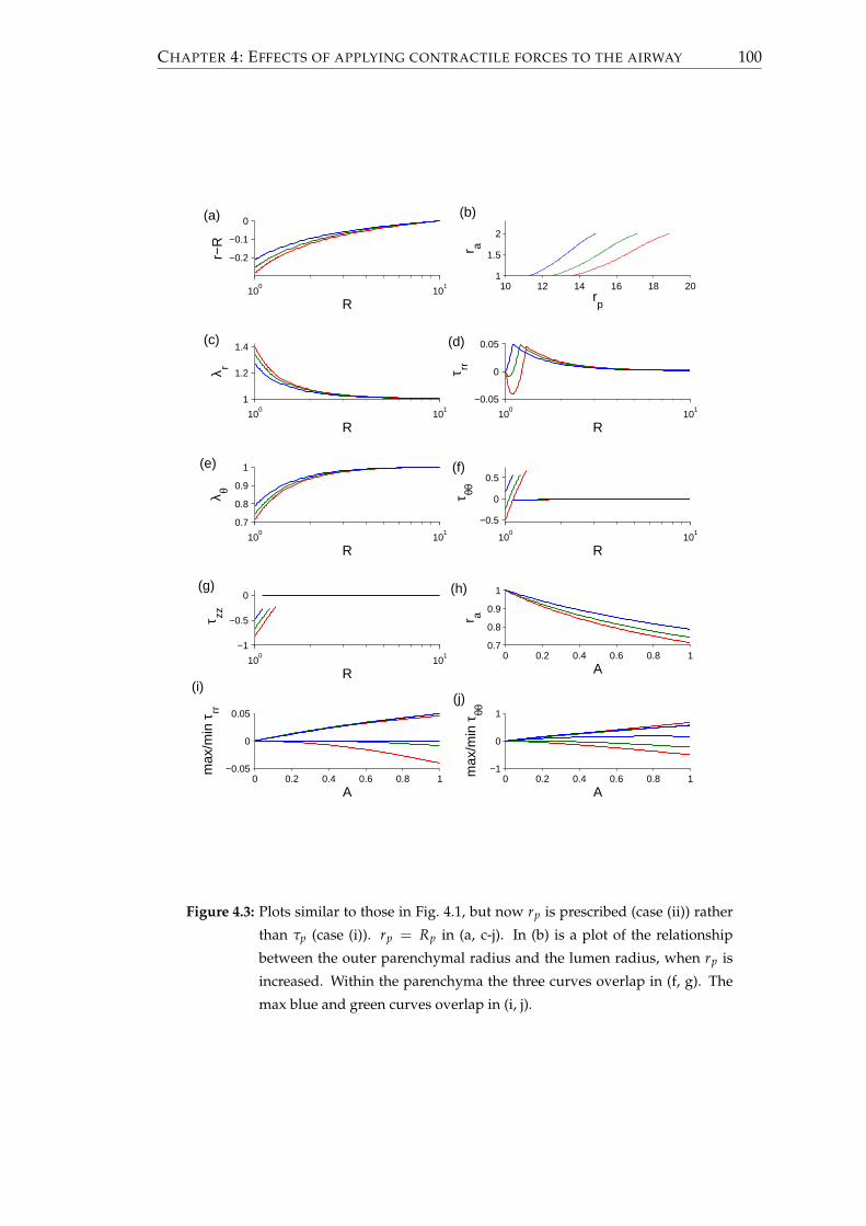
CHAPTER 4: EFFECTS OF APPLYING CONTRACTILE FORCES TO THE AIRWAY 100
100
101
−0.2
−0.1
0
R
r−R
10 12 14 16 18 201
1.5
2
rp
r a
100
101
1
1.2
1.4
R
λ r
100
101
−0.05
0
0.05
R
τrr
100
101
0.7
0.8
0.9
1
R
λ θ
100
101
−0.5
0
0.5
R
τθθ
100
101
−1
−0.5
0
R
τzz
0 0.2 0.4 0.6 0.8 10.7
0.8
0.9
1
A
r a
0 0.2 0.4 0.6 0.8 1−0.05
0
0.05
A
max
/min
τrr
0 0.2 0.4 0.6 0.8 1−1
0
1
A
max
/min
τθθ
(a)
(c)
(i)(j)
(f)
(d)
(b)
(e)
(g) (h)
Figure 4.3: Plots similar to those in Fig. 4.1, but now rp is prescribed (case (ii)) rather
than τp (case (i)). rp = Rp in (a, c-j). In (b) is a plot of the relationship
between the outer parenchymal radius and the lumen radius, when rp is
increased. Within the parenchyma the three curves overlap in (f, g). The
max blue and green curves overlap in (i, j).

CHAPTER 4: EFFECTS OF APPLYING CONTRACTILE FORCES TO THE AIRWAY 101
ated with the viscoelasticity can be ignored for the steady state solution. The differences
between this semi-nonlinear model and the fully-nonlinear model (Fig. 4.4) are much
less than those between the fully-linear model and the fully-nonlinear model (Fig. 4.2).
The findings of the two different cases for the boundary condition at R = Rp are very
similar. There is slightly more contraction in the case of the linear parenchyma model
(Fig. 4.4(a, e)). Where they are positive, the maximum and minimum stresses are a bit
lower with the semi-linear model than with the fully-nonlinear model, but when they
are negative, the maximum and minimum stresses are smaller in magnitude with the
fully-nonlinear model (b-d, f-h). The stresses are not as closely matched as the lumen
displacement, with the difference between the fully and semi-nonlinear models being
most noticeable for the maximum value of the radial stress (b,f).
In this section it has been shown that thicker walls contract to a greater extent. This is
physiologically significant, since wall thickening is an outcome of remodelling that is
characteristic of asthma. These results show that asthmatics can expect greater prob-
lems with breathing, with increased difficulty for those with severe asthma for whom
the airways are thickest [89]. Increasing the force produced by the ASM, as might oc-
cur in the case of a larger agonist concentration, also leads to increased levels of airway
narrowing.
4.2 Coupling to the crossbridge mechanics
We now consider the airway wall embedded in viscoelastic parenchyma, where the
airway wall mechanics are coupled to the crossbridge mechanics. The equations from
Sec. 2.3.3 are used to do this.
4.2.1 Model development
First the relevant equations are developed. Using the fact that rdr/dt=rbdrb/dt, the
tissue velocity, (2.3.16), may be written as
V =cos2 ϕrb
R√
(r2b − R2
b) cos2 ϕ + R2
drb
dt. (4.2.1)
Now in order to calculate rbdrb/dt, dA/dt will be required. Letting a(x) = (0, 0, x, x),
multiplying (2.3.10) through by βa and integrating with respect to x yields
β∫ ∞
−∞a(x) · ∂n
∂tdx + βγV
∫ ∞
−∞a(x) · ∂n
∂xdx = β
∫ ∞
−∞a(x) ·Qndx. (4.2.2)

CHAPTER 4: EFFECTS OF APPLYING CONTRACTILE FORCES TO THE AIRWAY 102
0 0.5 1
−0.25−0.2
−0.15−0.1
−0.05
A
r a−1
0 0.5 1−0.02
0
0.02
0.04
A
max
/min
τrr
0 0.5 1−0.4
−0.2
0
0.2
0.4
A
max
/min
τθθ
0 0.5 1
−0.6
−0.4
−0.2
0
Am
ax/m
in τ
zz
(d)(c)
(b)(a)
0 0.5 1
−0.2
−0.1
0
A
r a−1
0 0.5 1−0.02
0
0.02
0.04
A
max
/min
τrr
0 0.5 1−0.4
−0.2
0
0.2
0.4
A
max
/min
τθθ
0 0.5 1
−0.6
−0.4
−0.2
0
A
max
/min
τzz
(f)
(h)
(e)
(g)
Figure 4.4: Plots of (a, e) the displacement of the lumen, and the maximum and min-
imum values of (b, f) the radial stress, (c, g) the hoop stress and (d, h) the
axial stress in the airway wall verses contractile force A, when the non-
linear model is used for the parenchyma (solid) or its linearised version
(dashed). The airway wall is modelled nonlinearly in both cases. τp = 0
in (a-d), while rp = Rp in (e-h). The other parameter values are given in
Table 4.1.

CHAPTER 4: EFFECTS OF APPLYING CONTRACTILE FORCES TO THE AIRWAY 103
Parameter Comments
k1 3.5 t < 0.5
k1 0.6 t > 0.5
k2 1
k5 1
k6 3.5 t < 0.5
k6 0.6 t > 0.5
fp1 8.8
gp1 2.2
gp2 44
gp3 6.6
g1 0.1
g2 2
g3 0.3
Table 4.2: Rate parameters used to solve HHM. The rates, which were taken from
[116], have been nondimesionalised by dividing through by k∗2 = 0.1, with
the times multiplied by k∗2.
Since nC = nD = 0 at x = ±∞, integrating the second term on the left hand side by
parts gives∂A∂t
= β (H1 + γVH2) , (4.2.3)
where
H1 ≡∫ ∞
−∞a(x) ·Qn dx, H2 ≡
∫ ∞
−∞
∂a(x)∂x
· n dx. (4.2.4)
The equations governing the evolution of r in the parenchyma are now described. For
case (i), when the outer parenchymal stress is prescribed and nondimensionalising time
with respect to T∗ = 1/k∗2, (3.3.6) becomes[
t2tc∂
∂t+ 1
](r(R, t)− R) =
[t2
∂
∂t+ 1
] [B2(R)τp(t)− B1(R)τb(t)
], (4.2.5)
where, from (3.1.8),
τb =τa − log(
rb
raRb
)+
(r2a − 1)(R2
b − 1)2r2
ar2b
+ 2 cos2 ϕ∫ Rb
1
AR
dR
+ H(rb − Rb)C1
√π
C2cos2 ϕ
[erfi
(√C2(r2
a − 1) cos2 ϕ)
− erfi
(√C2
(r2a − 1)R2
bcos2 ϕ
) ], (4.2.6)
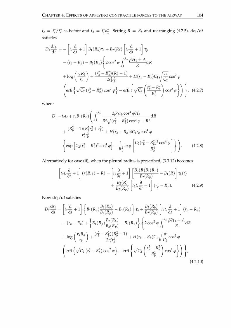
CHAPTER 4: EFFECTS OF APPLYING CONTRACTILE FORCES TO THE AIRWAY 104
tc = t∗c /t∗r as before and t2 = t∗r k∗2. Setting R = Rb and rearranging (4.2.5), drb/dt
satisfies
D1drb
dt=−
[t2
ddt
+ 1]
B1(Rb)τa + B2(Rb)[
t2ddt
+ 1]
τp
− (rb − Rb)− B1(Rb)
2 cos2 ϕ
∫ Rb
1
βH1 + AR
dR
+ log(
raRb
rb
)+
(r2b − R2
b)(R2b − 1)
2r2ar2
b+ H(rb − Rb)C1
√π
C2cos2 ϕ
(erfi
√C2
(r2
b − R2b)
cos2 ϕ− erfi
√C2
(r2
b − R2b
R2b
)cos2 ϕ
) , (4.2.7)
where
D1 =t2tc + t2B1(Rb)
( ∫ Rb
1
2βγrb cos4 ϕH2
R2√
(r2b − R2
b) cos2 ϕ + R2dR
+(R2
b − 1)(R2br2
a + r2b)
r4ar3
b+ H(rb − Rb)4C1rb cos4 ϕ
exp
[C2(r2
b − R2b)
2 cos4 ϕ]− 1
R2b
exp
[C2(r2
b − R2b)
2 cos4 ϕ
R4b
] ). (4.2.8)
Alternatively for case (ii), when the pleural radius is prescribed, (3.3.12) becomes[
t2tc∂
∂t+ 1
](r(R, t)− R) =
[t2
∂
∂t+ 1
] [B2(R)B1(Rp)
B2(Rp)− B1(R)
]τb(t)
+B2(R)B2(Rp)
[t2tc
∂
∂t+ 1
](rp − Rp). (4.2.9)
Now drb/dt satisfies
D2drb
dt=
[t2
ddt
+ 1]
B1(Rp)B2(Rb)B2(Rp)
− B1(Rb)
τa +B2(Rb)B2(Rp)
[t2tc
ddt
+ 1]
(rp − Rp)
− (rb − Rb) +
B1(Rp)B2(Rb)B2(Rp)
− B1(Rb)
2 cos2 ϕ∫ Rb
1
βH1 + AR
dR
+ log(
raRb
rb
)+
(r2b − R2
b)(R2b − 1)
2r2ar2
b+ H(rb − Rb)C1
√π
C2cos2 ϕ
(erfi
√C2
(r2
b − R2b)
cos2 ϕ− erfi
√C2
(r2
b − R2b
R2b
)cos2 ϕ
) ,
(4.2.10)

CHAPTER 4: EFFECTS OF APPLYING CONTRACTILE FORCES TO THE AIRWAY 105
where
D2 =t2tc − t2
B1(Rp)
B2(Rb)B2(Rp)
− B1(Rb) ( ∫ Rb
1
2βγrb cos4 ϕH2
R2√
(r2b − R2
b) cos2 ϕ + R2dR
+(R2
b − 1)(R2br2
a + r2b)
r4ar3
b+ H(rb − Rb)4C1rb cos4 ϕ
exp
[C2(r2
b − R2b)
2 cos4 ϕ]− 1
R2b
exp
[C2(r2
b − R2b)
2 cos4 ϕ
R4b
] ). (4.2.11)
A simplification to using the linear viscoelastic model for the parenchyma is to use a
linear elastic model. The elastic case is found by taking the limit t2 → 0. For case (i),
where the pleural stress is prescribed, taking the limit of (4.2.5) yields
r(R, t)− R =[
B2(R)τp(t)− B1(R)τb(t)]. (4.2.12)
Differentiating and rearranging yields
D3drb
dt= −B1(Rb)
(dτa
dt+ 2 cos2 ϕ
∫ Rb
1
βH1
RdR
)+ B2(Rb)
dτp
dt, (4.2.13)
where
D3 =1 + B1(Rb)
( ∫ Rb
1
2βγrb cos4 ϕH2
R2√
(r2b − R2
b) cos2 ϕ + R2dR
+(R2
b − 1)(r2a R2
b + r2b)
r3br4
a+ H(rb − Rb)4C1rb cos4 ϕ
exp
[C2(r2
b − R2b)
2 cos4 ϕ]− 1
R2b
exp
[C2
(r2b − R2
b)2
R4b
cos4 ϕ
] ). (4.2.14)
Alternatively for case (ii), when the pleural radius is prescribed, taking the limit t2 → 0
of (4.2.9) yields
r− R =[
B2(R)B1(Rp)B2(Rp)
− B1(R)]
τb(t) +B2(R)B2(Rp)
(rp − Rp). (4.2.15)
Differentiating and rearranging yields
D4drb
dt=
B1(Rp)
B2(Rb)B2(Rp)
− B1(Rb) (
dτa
dt+ 2 cos2 ϕ
∫ Rb
1
βH1
RdR
)+
B2(Rb)B2(Rp)
drp
dt,
(4.2.16)
where
D4 =1−
B1(Rp)B2(Rb)B2(Rp)
− B1(Rb) ( ∫ Rb
1
2βγrb cos4 ϕH2
R2√
(r2b − R2
b) cos2 ϕ + R2dR
+(R2
b − 1)(r2a R2
b + r2b)
r3br4
a+ H(rb − Rb)4C1rb cos4 ϕ
exp
[C2(r2
b − R2b)
2 cos4 ϕ]− 1
R2b
exp
[C2
(r2b − R2
b)2
R4b
cos4 ϕ
] ). (4.2.17)

CHAPTER 4: EFFECTS OF APPLYING CONTRACTILE FORCES TO THE AIRWAY 106
Figure 4.5: Outline of the setup of the airway problem for case (ii) with an elastic
parenchyma. Case (i) and the cases when the parenchyma is viscoelastic
are similar.
If rb is known for a given time, the deformed radius and stresses for each of the points
within the airway wall can be found using (2.2.18) and (3.1.9). The stresses within the
parenchyma can be found using (2.2.40).
4.2.2 Numerical methods
We now outline the structure of the problem and how we go about solving it (further
details are shown in Appendix B). R appears parametrically in n = n(x, t; R), A =
A(t; R),H1 = H1(t; R),H2 = H2(t; R) and V = V(t; R), while t appears parametrically
in r = r(R; t), rb = rb(t) and drb/dt = drb(t)/dt. Details of how they feed into one
another are shown in Fig. 4.5.
We discretise the airway wall in the radial direction into points spaced by a distance ∆R.
Given a crossbridge distribution at each point, A, H1 and H2 can be found. Modelling
the parenchyma with linear elasticity, the values of A, H1 and H2, at each of the points
in R, at the current time, can be used to find the values of rb and ∂rb/∂t analytically.
(If instead the parenchyma was assumed to be nonlinearly elastic, in order to satisfy
the boundary condition, it would be necessary to shoot across the parenchyma to find
rb and dr/dt, which could no longer be found analytically. This would lead to the
possibility of additional instability when finding ∂rb/∂t.) Having found rb and ∂rb/∂t
it is possible to find the new velocity at each of the discretised points in R. This is
used to decide on a timestep for a second order Godunov algorithm, used to update
the crossbridge populations n for each of the discretised points in R.
If the parenchyma is viscoelastic, rb and drb/dt must be updated numerically. This is

CHAPTER 4: EFFECTS OF APPLYING CONTRACTILE FORCES TO THE AIRWAY 107
χ Rp $ β τa ν(p) tc t2
0.2 10 3/26 2 0 0.3 4 0.1
Table 4.3: The standard parameter values for Sec. 4.3 and Sec. 4.4.
done using a midpoint method (See Appendix B.2).
4.3 Airway with prescribed time-dependent forcing
Although it is assumed that the velocity of the deformations affects the size of the con-
tractile force, before considering the fully coupled system, we first study an interme-
diate case. To find the steady state it was assumed that A was uniform and steady. In
this section A is prescribed to be time-dependent. In the next two subsections we solve
to find the evolution of the stresses and displacement as the airway contracts when the
parenchyma is elastic or viscoelastic. The effect of varying the parameters β, tc and t2
is also considered.
Rather than simply choosing A arbitrarily, we determine A(t) by solving the Huxley-
Hai-Murphy model for the isometric case. For an isometric contraction, V = 0 so
(2.3.10) reduces to∂n∂t
= Qn, (4.3.1)
thus there is a system of ordinary differential equations. Since the velocity is indepen-
dent of R, the solution of (4.3.1) will also be independent of R. Having discretised x as
described in Appendix B.1, ode45 in MATLAB can be used to solve (4.3.1). The stresses
and displacements can then be found as described in Sec. 4.2 (If the parenchyma is as-
sumed to be viscoelastic, (4.2.7) or (4.2.10) should be solved simultaneously to (4.3.1),
depending on the boundary conditions used.) An example of the time-dependence of
A is shown in figure 4.6. There is an initial rapid increase, before it levels off and ap-
proaches some steady state. This shows that when agonist is present, ASM can rapidly
produce, and then sustain, a contractile force.
4.3.1 Contraction with elastic parenchyma
If both the airway wall and the parenchyma are elastic, any deformations are quasi-
static, so as A evolves the airway responds instantaneously. The resulting distributions
are of the form seen in Fig. 4.1 if simulations are run for case (i) with zero pleural
stress, or Fig. 4.3 if simulations are run for case (ii) with zero pleural displacement.

CHAPTER 4: EFFECTS OF APPLYING CONTRACTILE FORCES TO THE AIRWAY 108
0 2 4 6 8 100
0.2
0.4
0.6
0.8
t
AFigure 4.6: Value of A when β = 2 and the rate parameters are as in Table 4.2.
Fig. 4.7 visualises and compares the evolution of the contraction of the airway under
the two different boundary conditions. Here the lumen radius and the maximum and
minimum principal stresses within the airway wall are shown against time. There are
no major differences between the curves for the two cases. With the exception of the
minimum values of the radial and hoop stresses, there is an initial rapid increase in
the magnitude of the displacement or the stress (the axial stress is negative), before
the magnitude of the displacement or stress levels off and approaches an equilibrium.
For small t, τrr = 0 (a) and τθθ > 0 (c), but as t increases they both become negative,
producing increased stress heterogeneity. They then rapidly increase in magnitude
before levelling off. The contraction is slightly less with case (ii) and the maximum
and minimum stresses are slightly greater in magnitude if they are tensile, but slightly
smaller in magnitude if they are contractile. These comparisons are found, since case
(ii) is equivalent to having a small radial stress on the pleura, whereas with case (i) it is
assumed that there is no radial stress at the pleura. These results show that during an
asthma exacerbation, assuming there are no oscillations due to breathing, there is an
initial rapid of narrowing of the airways, which then remain contracted.
In Fig. 4.7 we had set β = 2, where β depends on a number of factors (Sec. 2.3.2), in-
cluding the stiffness of the crossbridges and the area fraction of ASM fibres within the
airway wall. We now show the effect of altering β. Assuming case (ii) with zero pleu-
ral displacement, the evolution of the lumen radius and the maximum and minimum
stresses within the airway wall are shown in figure 4.8 for three values of β. Increasing
the value of β results in greater contractions (a). The stresses are also more heteroge-
neous and regions of compressive radial and hoop stresses (b, c) are predicted to arise
earlier, due to larger contractile forces. Simulations for case (i) with zero pleural stress
yield similar plots. These results therefore show that the larger the area fraction of the
ASM following airway wall remodelling, the narrower the airway can become.

CHAPTER 4: EFFECTS OF APPLYING CONTRACTILE FORCES TO THE AIRWAY 109
0 5 10−0.25
−0.2
−0.15
−0.1
−0.05
0
t
r a−1
0 5 10−0.01
0
0.01
0.02
0.03
t
max
/min
τ rr
0 5 10−0.2
0
0.2
0.4
t
max
/min
τ θθ
0 5 10−0.6
−0.4
−0.2
0
t
max
/min
τ zz
(d)
(b)
(c)
(a)
Figure 4.7: Figure comparing contractions with zero stress (case (i), dashed) or zero
displacement at R = Rp (case (ii), solid). Curves show the evolution of
(a) the lumen displacement, and (b-d) the maximum and minimum radial,
hoop and axial stresses as the airway contracts. Other parameter values
are given in Table 4.3, while the HHM rates are given in Table 4.2.

CHAPTER 4: EFFECTS OF APPLYING CONTRACTILE FORCES TO THE AIRWAY 110
0 5 10
−0.25
−0.2
−0.15
−0.1
−0.05
0
t
r a−1
0 5 10−0.02
0
0.02
0.04
tm
ax/m
in τ rr
0 5 10−0.4
−0.2
0
0.2
0.4
0.6
t
max
/min
τ θθ
0 5 10−0.8
−0.6
−0.4
−0.2
0
t
max
/min
τ zz
(d)(c)
(b)(a)
Figure 4.8: Curves showing the effect of changing β, where β depends on a number
of factors, including the stiffness of the crossbridges and the area fraction
of ASM fibres within the airway wall. β = 1 (red), 2 (green) or 3 (blue).
Curves show the evolution of (a) the lumen displacement, and (b-d) the
maximum and minimum radial, hoop and axial stresses, as the airway con-
tracts. Other parameter values are given in Table 4.3, while the HHM rates
are given in Table 4.2.

CHAPTER 4: EFFECTS OF APPLYING CONTRACTILE FORCES TO THE AIRWAY 111
4.3.2 Contraction with viscoelastic parenchyma
Having considered the limiting case for which the parenchyma is elastic, we now con-
sider the more general case in which the parenchyma is viscoelastic, which is more
representative of reality. We will concentrate on case (ii), where there is zero pleural
displacement, so rp = Rp. With the viscoelastic parenchyma, the following two param-
eters must be considered: tc = t∗c /t∗r , the ratio of the creep and relaxation timescales,
and t2 = k∗2t∗r , the the ratio of the relaxation timescale to the timescale for dephospho-
rylation of crossbridges. In Sec. 3.3.2 we set tc = 4, while from [135] we expect the
stress relaxation time to be approximately one second, so set t2 = 0.1.
Plots of the lumen displacement and maximum and minimum principal stresses within
the airway wall, when a contraction is applied are shown in Fig. 4.9 (solid). Also shown
are the corresponding curves when the parenchyma is elastic (dashed). The rate of con-
traction of the airway is slightly reduced when the parenchyma is viscoelastic rather
than elastic (a), but at large times the results are equivalent. Similarly the stresses are
the same at large times, but there are a number of differences at small times. Consider-
ing the radial stress (b), with the viscoelastic model the maximum value initially rises
rapidly, before peaking and decreasing a little, before once again rising and levelling
off, while the minimum value remains equal to zero for longer. The minimum value
of the hoop stress (c) also increases significantly initially, before decreasing and becom-
ing negative. The rate of decrease in the axial stress is reduced with the viscoelastic
parenchyma (d). From a physical viewpoint, assuming viscoelasticity, as a stress is ap-
plied to the inner boundary of the parenchyma, creep is expected to occur. Initially,
therefore the parenchyma does not displace as far as with the elastic parenchyma,
which in turn limits the displacement of the airway wall. Meanwhile as the airway
wall is displaced there is an initial build up of the stresses, which then reduce due to
stress relaxation. These results again predict that during an asthma exacerbation, as-
suming there are no oscillations due to breathing, there is an initial rapid of narrowing
of the airways, which then remain contracted.
Since the parameter value for the relaxation timescale was not measured in humans
and the ratio of the creep and relaxation timescale was only a rough estimate, the effect
of varying tc and t2 is now investigated. The effect of varying tc, the ratio of the creep
timescale to the relaxation timescale, is shown in Fig. 4.10. The larger the value of tc
the more pronounced the phenomena observed in Fig. 4.9 are and the contraction also
occurs slightly slower. The initial peak of the maximum radial stress is larger and com-
pressive stresses are only seen at later times (b). The minimum hoop stress is also larger
(c) and there can also be an initial peak in the maximum value of the hoop stress (c).

CHAPTER 4: EFFECTS OF APPLYING CONTRACTILE FORCES TO THE AIRWAY 112
0 5 10−0.25
−0.2
−0.15
−0.1
−0.05
0
t
r a−1
0 5 10−0.01
0
0.01
0.02
0.03
t
max
/min
τ rr
0 5 10−0.2
0
0.2
0.4
t
max
/min
τ θθ
0 5 10−0.6
−0.4
−0.2
0
t
max
/min
τ zz
(d)
(b)(a)
(c)
Figure 4.9: Curves show the evolution of the lumen displacement (a), and (b-d) the
maximum and minimum radial, hoop and axial stresses as the airway con-
tracts, with rp = Rp (case (ii)). The parenchyma is either viscoelastic (solid)
or elastic (dashed). Other parameter values are given in Table 4.3, while the
HHM rates are given in Table 4.2.

CHAPTER 4: EFFECTS OF APPLYING CONTRACTILE FORCES TO THE AIRWAY 113
A very small peak also exists for small time for the axial stress when tc = 10 (d, blue).
Larger values of tc correspond to larger values of the creep timescale, thus indicating
a slower response of the parenchyma to the added stress, due to the contractile force.
This allows for a greater build up in the initial radial and hoop stresses.
The effect of varying t2, the ratio of the relaxation timescale to the timescale for dephos-
phorylation of crossbridges, is shown in Fig. 4.11. For small values of t2 the results are
similar to those of an elastic parenchyma, which is the limit case that t2 → 0 (dots).
However, as t2 increases, the viscoelastic phenomenae become more prominent. As
well as just increasing the size of the initial peaks, increasing t2 also slows the rate of
convergence to the equilibrium state. So for example, when t2 = 1, the maximum value
of the radial stress no longer peaks before decreasing, then rising again to the equilib-
rium solution; rather it simply slowly decreases to the equilibrium after peaking (b,
blue). Physically, decreasing t2 relates to decreasing the relaxation timescale, therefore
any increase in the radial or hoop stresses, due to the slowness of the parenchymal
response, will decay more quickly and so not build up as much.
4.4 Airway coupled to HHM model
Having prescribed A as some time-dependent function, by solving the HHM equations
for an isometric contraction, we now use the fully coupled HHM model to find A. This
enables the velocity of contraction to feed back into crossbridge populations evolution
and means that in general A is no longer uniform. We again adopt the nonlinear fibre-
reinforced model for the airway wall and consider both the linear elastic and linear
viscoelastic models of the parenchyma. For this section we focus on case (ii), where
the pleural radius is prescribed. Again unless otherwise stated, the parameters for this
section are given in Table 4.3.
Plots are shown in Fig. 4.12 for a contracting airway when either the parenchyma is
elastic (blue) or viscoelastic (green). (In reality the parenchyma is viscoelastic.) The
pleural boundary is held so that rp = Rp. At large time, the lumen displacement and
the maximum and minimum stresses are the same as those found in the previous sec-
tion, where A was prescribed by solving HHM in the isometric case (red). However,
these equilibrium solutions are now reached a lot slower having coupled the contin-
uum model fully to HHM. Again, when the parenchyma is viscoelastic, the contrac-
tion is slower (a) and there are initial peaks in the maximum radial stress (b) and the
hoop stress (c). The axial stress also reduces more slowly (d). While the equilibrium
solution has attached crossbridges only within the region 0 < x < 1, as the airway

CHAPTER 4: EFFECTS OF APPLYING CONTRACTILE FORCES TO THE AIRWAY 114
0 5 10−0.25
−0.2
−0.15
−0.1
−0.05
0
t
r a−1
0 5 10
0
0.02
0.04
0.06
t
max
/min
τ rr
0 5 10−0.2
0
0.2
0.4
t
max
/min
τ θθ
0 5 10−0.6
−0.4
−0.2
0
t
max
/min
τ zz
(d)(c)
(a) (b)
Figure 4.10: Plots showing the effect of varying tc, the ratio of the creep and relaxation
timescales. Curves show the evolution of (a) the lumen displacement,
and (b-d) the maximum and minimum radial, hoop and axial stresses,
as the airway contracts, with tc = 2 (red), 4 (green) or 10 (blue). Other
parameter values are given in Table 4.3, while the HHM rates are given in
Table 4.2.

CHAPTER 4: EFFECTS OF APPLYING CONTRACTILE FORCES TO THE AIRWAY 115
0 5 10−0.25
−0.2
−0.15
−0.1
−0.05
0
t
r a−1
0 5 10
0
0.02
0.04
0.06
0.08
t
max
/min
τ rr
0 5 10−0.2
0
0.2
0.4
0.6
t
max
/min
τ θθ
0 5 10−0.6
−0.4
−0.2
0
t
max
/min
τ zz
(d)(c)
(a) (b)
Figure 4.11: Plots showing the effect of varying t2, the ratio of the relaxation timescale
to the timescale for dephosphorylation of crossbridges. Curves show the
evolution of (a) the lumen displacement, and (b-d) the maximum and
minimum radial, hoop and axial stresses as the airway contracts, with
t2 = 0.01 (red), 0.1 (green) or 1 (blue). Dots are the elastic limit case.
Other parameter values are given in Table 4.3, while the HHM rates are
given in Table 4.2.

CHAPTER 4: EFFECTS OF APPLYING CONTRACTILE FORCES TO THE AIRWAY 116
0 50 100−0.25
−0.2
−0.15
−0.1
−0.05
0
t
r a−1
0 50 100−0.01
0
0.01
0.02
0.03
t
max
/min
τ rr
0 50 100−0.2
0
0.2
0.4
t
max
/min
τ θθ
0 50 100−0.6
−0.4
−0.2
0
t
max
/min
τ zz
(d)
(b)
(c)
(a)
Figure 4.12: Curves of (a) the lumen displacement, and (b-d) the maximum and min-
imum radial, hoop and axial stresses for a contraction, when coupled
to HHM theory where the parenchyma is elastic (blue) or viscoelastic
(green), or when the contractile force is prescribed as in the previous
section and the parenchyma is elastic (red). Other parameter values are
given in Table 4.3, while the HHM rates are given in Table 4.2.
contracts they move out of this region. The approach to equilibrium is reached more
slowly, since these crossbridges must detach, while the number of crossbridge within
0 < x < 1 must build up. These results predict that during an asthma exacerbation, as-
suming there are no oscillations due to breathing, that rather than the airways initially
rapidly narrowing and then remaining contracted, as was predicted in the previous
subsection, they contract more steadily.

CHAPTER 4: EFFECTS OF APPLYING CONTRACTILE FORCES TO THE AIRWAY 117
4.4.1 Effect of including oscillatory forcing
We now consider the effect of displacing the outer boundary of the parenchyma. Start-
ing from the steady contracted state, oscillations of the following form are applied:
rp = Rp + a(
1− cos(
2πtP∗k∗2
)), (4.4.1)
where a is the amplitude of the oscillations and P∗ is the dimensional period of a cy-
cle. Physiologically it is reasonable to let P∗ = 5s. Unless otherwise stated, we let
a = 0.5, which at its peak corresponds to a 10% displacement of the pleura. Plots are
shown in Fig. 4.13 when the parenchyma is elastic. Initially there is a transient pe-
riod before equilibrium loops are approached. Introducing the oscillations results in a
reduction in the amount of contraction (a), with the red line joining the points of mini-
mum displacement in each cycle of oscillation. Similarly, the magnitude of the smallest
value, in each cycle of oscillation, of the maximum and minimum radial, hoop and ax-
ial stresses within the airway wall and the contractile force at the inner boundary of the
airway wall (red lines) get smaller (b-e). During each cycle, the oscillations increase the
range of values of the radial stress, while for a portion of each cycle, the radial stress
is purely tensile (b). Similarly the oscillations can cause the regions where the hoop
stress is compressive to become tensile (c). During the oscillations the crossbridges are
stretched further, which increases the contractile force that they produce; however, this
also results in more of them detaching. Over time the average force is thus reduced
(e). The range of velocities initially increases, before decreasing to an equilibrium, with
the velocity varying smoothly (f). Coupling the continuum model to the HHM model
in effect inparts viscoelastic properties to the airway wall, resulting in hysteresis (g).
These results are physiologically significant since they show that tidal breathing is able
to reduce the amount of airway contraction by a small amount.
The effect of varying the amplitude of the oscillations is shown in Fig. 4.14. The min-
imum value, in each cycle of oscillation, of each of the quantities, as was shown in
Fig. 4.13 by the red lines, are plotted. Increasing the amplitude of the oscillations re-
duces the magnitude of the stresses and the contraction of the airway. The only points
where this is not the case are for the the minimum radial stress (b) and the maximum
and minimum hoop stresses (c) at small time. In these cases, for the larger amplitudes
the stresses initially increase in magnitude before starting to decrease. This can be ex-
plained by the increased stretch of the attached crossbridges before they detach. These
results are consistent with the experimental findings of Fredberg et al. [43] and many
others, that revealed that application of length fluctuations to tissue strips causes the
mean contractile force to decrease. These results therefore predict that increasing the

CHAPTER 4: EFFECTS OF APPLYING CONTRACTILE FORCES TO THE AIRWAY 118
0 20 40−0.22
−0.2
−0.18
t
r a−1
0 20 400
0.05
0.1
t
max
/min
τ rr
0 20 40
0
0.5
1
t
max
/min
τ θθ
0 20 40
−0.4
−0.2
0
tm
ax/m
in τ zz
0 20 40
0.6
0.8
1
t
A(1
)
0 20 40−0.05
0
0.05
t
v(1)
(f)(e)
(d)(c)
(b)(a)
0.6 0.7 0.8
0.812
0.814
0.816
A(1)
r a−1
(g)
Figure 4.13: Curves of the evolution of (a) the lumen displacement, (b-d) the max-
imum and minimum radial, hoop and axial stresses, (e) the contractile
force and (f) the relative filament velocity at the inner boundary of the
airway wall. Starting from the contracted steady state, oscillations are ap-
plied to the pleural radius using (4.4.1) with a = 0.5. The red lines join
the minimum values in each cycle of oscillation. Also plotted (g) an equi-
librium curve, showing hysteresis, of the lumen displacement against the
inner contractile force. Other parameter values are given in Table 4.3,
while the HHM rates are given in Table 4.2.

CHAPTER 4: EFFECTS OF APPLYING CONTRACTILE FORCES TO THE AIRWAY 119
depth of breathing helps to reduce the level of contraction of the airways to a greater
extent. This suggests that deep breathing can be used as a protection method to reduce
the effects of asthma.
The effect of increasing the amplitude of the oscillations and then reducing them to the
previous value are shown in Fig. 4.15, with a = 0.5 for t ≤ 150 and 300 < t ≤ 450,
and a = 1 for 150 < t ≤ 300. When the amplitude of the oscillations returns to 0.5
again, the same level of contraction and the same stresses and contractile forces are ap-
proached as previously. This is not surprising as the equilibrium loops that are formed
do not take into account the history of previous oscillations. In order to match up to
the experimental findings of Fredberg et al. [44], that the airway remodels depending
on the conditions that are applied to it, it is necessary to adapt the model further. One
way to do this would be to use the techniques of Brook and Jensen [21], to allow for
remodelling of the structure of the contractile units within the ASM.
Finally, results are shown in Fig. 4.16 when oscillations of the form (4.4.1) are applied
to the airway, when the parenchyma is viscoelastic. In comparison to the results where
the parenchyma is elastic (Fig. 4.14), oscillations lead to a greater reduction in the level
of contraction (a). The range of displacements in each cycle of oscillation is also greater.
Similarly the range within a cycle of oscillation is greater for the stresses (b-d). At points
within the cycle the radial or hoop stresses can be purely tensile, while at other points
they can be purely compressive. There is also a greater reduction in the size of the con-
tractile force, which for a short period of the oscillations becomes negative indicating
that the crossbridges are resisting contraction (e). The range of velocities initially in-
creases before levelling off and the range is greater than with the elastic parenchyma
(f). These results are significant since they not only take into account the fact that the
parenchyma is viscoelastic, but show that tidal breathing can quite noticeably reduce
the level of contraction of the airways.
4.5 Comparisons to experimental data
We now make further comparisons to experimental data to test the validity of our
model, before making comparisons between the airway and the tissue strip in the next
section. In particular we consider the data of LaPrad et al. [103], for which experiments
were carried out on an airway dissected from the surrounding parenchyma. They de-
signed two protocols to test the significance of the tidal breathing and deep inspirations
on bronchoconstriction. They found that tidal oscillations have little effect on the mean
lumen radius in comparison to when there are no oscillations. We describe the methods

CHAPTER 4: EFFECTS OF APPLYING CONTRACTILE FORCES TO THE AIRWAY 120
0 20 40−0.22
−0.2
−0.18
−0.16
−0.14
t
r a−−
1
0 20 40−0.01
0
0.01
0.02
0.03
t
max
/min
τ rr−
0 20 40−0.2
0
0.2
0.4
t
max
/min
τ θθ−
0 20 40
−0.5
−0.4
−0.3
−0.2
−0.1
0
t
max
/min
τ zz−
(d)
(b)
(c)
(a)
0 10 20 30 40 50
0.4
0.5
0.6
0.7
t
A−(1
)
(e)
Figure 4.14: Curves joining the minimum values in each cycle of oscillation of (a) the
lumen displacement, (b-d) the maximum and minimum radial, hoop and
axial stresses and (e) the contractile force at the inner boundary. Oscilla-
tions are applied to the pleural radius using (4.4.1) with a = 0.25 (red),
0.5 (green), 0.75 (blue) and 1 (black). Arrows indicate increasing ampli-
tude oscillations. Other parameter values are given in Table 4.3, while the
HHM rates are given in Table 4.2.

CHAPTER 4: EFFECTS OF APPLYING CONTRACTILE FORCES TO THE AIRWAY 121
0 150 300 450−0.25
−0.2
−0.15
t
r− a−
1
0 150 300 450−0.01
0
0.01
0.02
0.03
t
max
/min
τ− rr
0 150 300 450−0.2
0
0.2
0.4
t
max
/min
τ− θθ
0 150 300 450
−0.4
−0.2
0
t
max
/min
τ− zz
(b)
(c)
(a)
(d)
0 150 300 4500.4
0.5
0.6
0.7
t
A−(1
)
(e)
Figure 4.15: Curves joining the minimum values in each cycle of oscillation of (a) the
lumen displacement, (b-d) the maximum and minimum radial, hoop and
axial stresses and (e) the contractile force at the inner boundary. Oscil-
lations are applied to the pleural radius using (4.4.1) with a = 0.5 for
t ≤ 150 and t > 300 and a = 1 for 150 < t ≤ 300. Other parameter values
are given in Table 4.3, while the HHM rates are given in Table 4.2.

CHAPTER 4: EFFECTS OF APPLYING CONTRACTILE FORCES TO THE AIRWAY 122
0 50
−0.2
−0.1
0
t
r a−1
0 50−0.2
0
0.2
0.4
t
max
/min
τ rr
0 50−1
0
1
2
t
max
/min
τ θθ
0 50−0.6−0.4−0.2
00.2
t
max
/min
τ zz
0 500
0.5
1
1.5
t
A(1
)
0 50−0.5
0
0.5
t
v(1)
(d)
(b)
(f)(e)
(c)
(a)
Figure 4.16: Curves of the evolution of (a) the lumen displacement, (b-d) the range of
the maximum (blue) and minimum (red) radial, hoop and axial stresses
in each cycle of oscillation, (e) the contractile force and (f) the relative
filament velocity at the inner boundary of the airway wall. Starting from
the contracted steady state, oscillations are applied to the pleural radius
using (4.4.1) with a = 0.5. The smallest value of max τrr and the largest
value of min τrr overlap. Other parameter values are given in Table 4.3,
while the HHM rates are given in Table 4.2.

CHAPTER 4: EFFECTS OF APPLYING CONTRACTILE FORCES TO THE AIRWAY 123
used to compare our model predictions and show the results.
4.5.1 Methods
Previously values were selected for C1 and C2 by fitting to the model of Lambert et
al. [98] (Sec. 3.1.3). We update these values by using the mean pressure-radius plot
shown in Fig. 8 of [103]. For ease of comparison with tissue strips, we assume the fibres
form hoops, so that ϕ = 0. Again assuming that µ(w)∗ = 20cmH20, we set C1 = 0.05
and C2 = 1.8 based on the fit with LaPrad et al. [103] data. We let χ = 0.3 for both
protocols.
We now briefly describe the two protocols of LaPrad et al. [103] and describe how we
mimic them.
• Protocol 1: LaPrad et al. [98] applied an initial transmural pressure of 7.5 cmH20
and every 12 minutes increased the concentration of Acetylcholine (ACh) applied
to the airway. During this process they either kept the transmural pressure static,
applied tidal oscillations or applied tidal oscillations with periodic deep inspi-
rations. They recorded the airway radius and thickness when the transmural
pressure was equal to 7.5 cmH20 when applying oscillations.
In order to mimic the increased agonist concentrations, we select the following
three values for k1 and k6 and let β = 5, so that at steady state the airway contracts
to approximately 95, 75 or 60% of the starting radius:
k1 = k6 =
0.05 if t ≤ 72,
0.25 if 72 < t ≤ 144,
0.5 if 144 < t ≤ 216.
(4.5.1)
Here, as in [52, 116], we have assumed that the rates of phosphorylation of
unattached and attached crossbridges are the same. Times have once again been
nondimesionalised with respect to 1/k∗2. We consider the static and tidal cases,
for which we let
[[τ]] =
38 (static),
38 + 1
8 sin( 2πt
0.5
)(tidal).
(4.5.2)
To ensure that there are no sudden changes in the velocity with the tidal simu-
lation, that could cause the numerical methods to become unstable, we ramp up
the amplitude of the oscillation over the first oscillation as follows:
[[τ]] =38
+18
(t
0.5
)sin
(2πt0.5
), for t ≤ 0.5. (4.5.3)

CHAPTER 4: EFFECTS OF APPLYING CONTRACTILE FORCES TO THE AIRWAY 124
Protocol χ β µ(w)∗ ϕ C1 C2
1 0.3 5 20cmH20 0 0.05 1.8
2 0.3 5 20cmH20 0 0.05 1.8
Table 4.4: The parameter values for Sec. 4.5.
• Protocol 2: LaPrad et al. [98] applied an initial transmural pressure of 5 cmH20
and then added 10−5 M ACh to the airway. They increased the peak-to-peak am-
plitude of sinusoidal oscillations to the transmural pressure every 15 minutes. For
the first 15 minutes there were no oscillations, then the amplitudes that followed
were 2.5, 5 and 10 cmH20.
We again let k1 = k6 = 0.25 and β = 5, which ensures that at steady state the air-
way radius is about 60% of its starting value, and apply the following transmural
pressures to the airway wall:
[[τ]] =
14 if t ≤ 90,
14 + 1
16 sin( 2πt
0.5
)if 90 < t ≤ 180,
14 + 1
8 sin( 2πt
0.5
)if 180 < t ≤ 270,
14 + 1
4 sin( 2πt
0.5
)if 270 < t ≤ 360.
(4.5.4)
Similar to protocol 1, we ramp up the size of the amplitude over the first cycle
each time, to ensure that there are no sudden changes in the velocity. Initially at
t = 0 the airway is said to be in the baseline state (B), while at t = 90, following
contraction, the airway is said to be in the contracted state (C).
We slightly adapt the rate of Mijailovich et al. [116] for g and take it to be ten times
larger as used by Wang et al. [173]. We normalise the radius by dividing ra by ra(0)
and we find the normalised wall thickness by dividing rb − ra by rb(0) − ra(0). The
strain amplitude is found by dividing max(ra)−min(ra) by 2ra(0). The strain amplitude
for the baseline and contracted states in protocol 2 are found by briefly oscillating the
transmural pressure with amplitude 1/16.
4.5.2 Results
Fig. 4.17 shows the plots of the radius normalised to the radius at t = 0 for the static
(a) and tidal (b) cases of protocol 1. In each case, as k1 increases, the airway contracts
further (c) and the wall gets thicker (d). Considering the airway radius, tidal oscilla-
tions reduce the level of contraction slightly when k1 = 0.05 or 0.5, while the difference

CHAPTER 4: EFFECTS OF APPLYING CONTRACTILE FORCES TO THE AIRWAY 125
is more pronounced when k1 = 0.25 (c). The results of LaPrad et al. [103] show little
difference in the radius in the two cases for each concentration of ACh. By considering
the evolution of the radius in (a, b), with the rate parameters that are used, the equi-
librium state has not yet been reached when k1 = 0.25, which could be causing the
difference here. There are similar differences with the airway thickness when k1 = 0.25
(d). For the tidal case, when k1 = 0.05, there is little difference in comparison to the
strain amplitude if k1 = 0 (e). However, for the larger values of k1, the strain amplitude
is much reduced. These findings for the strain amplitude are consistent with those in
[103] (h).
Fig. 4.18 shows the plots for protocol 2. Considering the evolution of the radius, each
time that the amplitude of the oscillations is increased, there is a large increase in the
radius, with the airway then gradually contracting once again (a). These features can
be explained by the increased value of g, which means that the latch crossbridges are
more likely to detach when they are stretched. However, considering the equilibrium
states of the radius (b), there is little reversal in the level of contraction for the two
smallest amplitudes of oscillations, with the results contained within the error bars of
the results shown in [103] (e). For the largest amplitude oscillations, the model predicts
greater reductions in the level of contraction than the experimental results of [103].
As the oscillation amplitude increases the airway thickens (c). The strain amplitude
is decreased following contraction and raises a small amount when the oscillations
with the smallest two amplitudes are applied, with a much greater increase in strain
amplitude for the largest amplitude oscillations (d). This is consistent with the results
in [103] (g).
Due to the issues observed in Fig. 4.18 with the increased value of g, the simulations
can be repeated with the original value for g. The results are shown in Fig. 4.19. There
are now no large deformations of the radius each time the amplitude of the oscillations
is increased (a) and there are now only small changes in the mean airway radius (b)
and thickness (c) when each amplitude of oscillations is applied, consistent with [103]
(Fig. 4.18 (e, f)). However, the model now no longer predicts such a large increase
in strain amplitude when the greatest amplitude oscillations are applied (d). In the
contracted state the airway is more contracted, which could be causing this.
4.5.3 Discussion
Overall the model predictions are consistent with the findings of LaPrad et al. [103],
which therefore gives credibility to our model. However, there are still questions about
what appropriate rate parameters for the HHM model are.

CHAPTER 4: EFFECTS OF APPLYING CONTRACTILE FORCES TO THE AIRWAY 126
072
144
216
0.6
0.81
normalised radius
072
144
216
0.6
0.81
time
normalised radius(a)
(b)
0
0.05
0.25
0.5
6080100
Radius (%)
0
0.05
0.25
0.5
100
150
200
Thickness (%)
0
0.05
0.25
0.5
0
2.55
k 1
Strain Ampitude (%)
0
10^−
710
^−6
10^−
510
^−4
10^−
3020406080100 0
10
^−7
10^−
610
^−5
10^−
410
^−3
100
200
300
400 0
10
^−7
10^−
610
^−5
10^−
410
^−3
0
2.55
AC
h D
ose
(M)
(d)
(e)
(f)
(g) (h
)
(c)
Figu
re4.
17:P
roto
col1
:Plo
tsof
the
norm
alis
edra
dius
agai
nstt
ime
for
the
(a)s
tati
can
d(b
)tid
altr
ansm
ural
pres
sure
.A
lso
show
nar
epl
ots
of
the
final
(c)l
umen
radi
us,(
d)ai
rway
thic
knes
san
d(e
)str
ain
ampl
itud
efo
rth
em
ean
tran
smur
alpr
essu
re,f
orea
chva
lue
ofk 1
for
the
stat
ic(c
ircl
es)
and
tida
l(cr
osse
s)ca
ses.
(f-h
)Th
eco
rres
pond
ing
plot
sfo
rth
era
dius
,thi
ckne
ssan
dst
rain
ampl
itud
ew
hen
the
expe
rim
enta
ldat
a[1
03]i
sus
ed.

CHAPTER 4: EFFECTS OF APPLYING CONTRACTILE FORCES TO THE AIRWAY 127
090
180
270
360
0.6
0.81
time
normalised radius
B
C
1/16
3/8
3/16
1/4
6080100
Radius (%)
B
C
1/16
3/8
3/16
1/4
100
150
200
Thickness (%)
B
C
1/16
3/8
3/16
1/4
0369
ampl
itude
Strain Ampitude (%)
B
C
1/16
3/8
3/16
1/4
6080100 B
C
1/
16 3
/83/
16 1
/410
0
150
200 B
C
1/
16 3
/83/
16 1
/40369
ampl
itude
(e)
(f) (g
)
(a)
(d)
(c)
(b)
Figu
re4.
18:P
roto
col2
:(a)
Plot
ofth
eno
rmal
ised
radi
usag
ains
ttim
e.A
lso
show
nar
epl
ots
of(b
)the
lum
enra
dius
,(c)
airw
ayth
ickn
ess
and
(d)
stra
inam
plit
ude
for
the
mea
ntr
ansm
ural
pres
sure
,for
each
valu
eof
the
ampl
itud
eof
the
tran
smur
alpr
essu
reos
cilla
tion
s.g 1
=1,
g 2=
20an
dg 3
=3.
(e-g
)The
corr
espo
ndin
gpl
ots
for
the
radi
us,t
hick
ness
and
stra
inam
plit
ude
whe
nth
eex
peri
men
tald
ata
[103
]
isus
ed.B
and
Cre
fer
toth
eba
selin
ean
dco
ntra
cted
stat
es.

CHAPTER 4: EFFECTS OF APPLYING CONTRACTILE FORCES TO THE AIRWAY 128
0 90 180 270 360
0.6
0.8
1
time
norm
alis
ed r
adiu
s
B C 1/16 3/8 3/16 1/4
60
80
100
Rad
ius
(%)
B C 1/16 3/8 3/16 1/4100
150
200
Thi
ckne
ss (
%)
B C 1/16 3/8 3/16 1/40
3
6
9
amplitude
Stra
in A
mpi
tude
(%
)
(c)
(a)
(d)
(b)
Figure 4.19: Protocol 2: (a) Plot of the normalised radius against time. Also shown are
plots of the (b) lumen radius, (c) airway thickness and (d) strain ampli-
tude for the mean transmural pressure, for each value of the amplitude of
the transmural pressure oscillations. g1 = 0.1, g2 = 2 and g3 = 0.3. B and
C refer to the baseline and contracted states.
One of the main conclusions of LaPrad et al. [103] is that introducing tidal breathing
does not significantly alter the level of contraction of the airway. However, there are
a number of questions about the results that they found. For example, they have car-
ried out experiments where the airway is dissected from the parenchyma, which could
have an important impact in vivo. For instance, in the previous section, the model
predicted that if the airway was embedded within elastic parenchyma, applying oscil-
latory boundary conditions resulted in small changes to the airway radius (Fig. 4.14).
However, when embedded within viscoelastic parenchyma, applying the same oscilla-
tory boundary conditions resulted in much larger reductions in the amount of airway
contraction.
4.6 Comparisons of airway with tissue strip
Finally, we make a few comparisons between the airway and the tissue strip. We in-
troduce a simple model of the tissue strip and the relevant numerical methods, before
showing results.

CHAPTER 4: EFFECTS OF APPLYING CONTRACTILE FORCES TO THE AIRWAY 129
4.6.1 Modelling a tissue strip
We model the strip as closely as possible to mimic the airway wall (Sec. 2.2). It is
assumed that the tissue strip is long and thin, since the strips used by Fredberg et
al. [43] measured 2 x 3 x 20mm. As the length is much greater than the height and
width, which are roughly equal, any boundary layers at the ends, that arise due to
clamping, are ignored.
Considering a strip of unstressed equilibrium length L∗u subject to uniaxial strain,
x∗ = λ1X∗, y∗ = λ1Y∗, s∗ = λS∗, (4.6.1)
Here X∗, Y∗, S∗ are Lagrangian Cartesian coordinates and x∗, y∗, s∗ are coordinates
in the deformed configuration. (S∗ is used, so as not to be confused with Z∗ in the
airway.) F =diag(λ1, λ1, λ), so assuming incompressibility, as assumed for the airway
wall, λλ21 = 1, implying that λ1 = 1/
√λ. Now B = C =diag(1/λ, 1/λ, λ2).
Since the smooth muscle fibres form rings in the trachea, we assume that both sets of
fibres are aligned to the s-axis of the strip, meaning M1 = M2 = es. In the deformed
configuration m1 = m2 = λes, thus the anisotropic invariants satisfy I4 = I6 = λ2.
The same strain-energy function as was used for the airway wall (see (2.2.7)) is used.
However, lengths are now nondimensionalised by L∗u, so that
W =I1 − 3
2+ H(λ− 1)
C1
C2
(exp
[C2
(λ2 − 1
)2]− 1
)+ Aλ2. (4.6.2)
The non-zero components of the Cauchy stress tensor are
τxx = τyy = −p +1λ
, (4.6.3)
τss = −p + λ2(1 + 2A) + H(λ− 1)4C1(λ2 − 1)λ2 exp[C2(λ2 − 1)2] . (4.6.4)
Assuming that the sides of the strip are stress-free, p = 1/λ and
τxx = τyy = 0, (4.6.5)
τss = λ2(1 + 2A)− 1λ
+ H(λ− 1)4C1(λ2 − 1)λ2 exp[C2(λ2 − 1)2] . (4.6.6)
Conservation of momentum is satisfied and
x =X√
λ, y =
Y√λ
, s = λS. (4.6.7)
We assume that λ is being prescribed, however, an alternative is that τss is prescribed.

CHAPTER 4: EFFECTS OF APPLYING CONTRACTILE FORCES TO THE AIRWAY 130
4.6.2 Numerical methods for the tissue strip
If λ is prescribed, then V can immediately be found at each time step. The Godunov
scheme (Appendix B.1) is used to update n and thus A, from which τss is given by
(4.6.6). Alternatively if τss is prescribed, a similar method can be used as shown in
Fig. 4.5 for the airway. Instead of rb, we now solve for λ. Differentiating (4.6.6) and
using (4.2.3), rearranging gives
V(t) =∂λ
∂t=
∂τss/∂t− 2λ2βH1
2λ(1 + 2A) + 2λ2βγH2 + λ−2 + H(λ− 1)E, (4.6.8)
where
E = 4C1 exp(
C2(λ2 − 1
)2) [
2λ3 + 2λ(λ2 − 1
) 1 + 2C2
(λ2 − 1
)λ2]
. (4.6.9)
4.6.3 Results
In Sec. 4.5.2, results were shown when the protocols of LaPrad et al. [103] were mim-
icked. Results were shown for the airway radius and thickness and the strain ampli-
tude, but not the stress. For these results it was assumed that the fibres formed hoops
with ϕ = 0, meaning that the stress that the fibres experienced was τθθ . Comparisons
are now made between the airway and the strip by applying the same stretch to the
tissue strip as was experienced by the fibres at the mid point within the airway wall.
The values for k1 are also assumed to be the same.
Fig. 4.20 shows the stress that the fibres experience at the inner and outer boundaries
of the airway wall and in the strip, when protocol 1 is applied. Also plotted is the
relationship between the stretch of the fibres in the strip (equal to the stretch of the
fibres at the mid point of the airway wall) and the stresses, for each value of k1 (b-d). In
each of the cases, the stress experienced by the fibres within the strip is similar to that
of the fibres at the outer boundary of the airway wall, and is quite different from the
stress of the fibres at the inner boundary of the airway wall.
Fig. 4.21 shows the results for protocol 2 when g takes either the value as described in
[116] or ten times this value as used in [173]. Unlike protocol 1, where the stress within
the strip was always within the range of stresses experienced in the airway wall, with
protocol 2 this is not always the case (d). At some points within the equilibrium loops
the fibres at the inner boundary of the airway can be under compression, while those
at the outer boundary are under tension. Such heterogeneities are not seen within the
strip for which there is a single stress along its length.
These results therefore show that due to the simplified geometry of the tissue strip,

CHAPTER 4: EFFECTS OF APPLYING CONTRACTILE FORCES TO THE AIRWAY 131
0 0.05 0.25 0.5 0
2
4
6
k1
stre
ss
1.28 1.33 1.380
2
4
6
8
stretch
stre
ss
1.05 1.055 1.060
1
2
3
stretch0.874 0.877 0.880
1
2
stretch
(c) (d)
(a)
(b)
Figure 4.20: Protocol 1: (a) Plots of the stress within the fibres in the strip (blue) and the
inner (red) and outer (green) boundaries of the airway, when the trans-
mural pressure is static (solid) or tidal (dashed). Also plots of fibre stretch
against the reference fibre stretch when (b) k1 = 0.05, (c) k1 = 0.25 and (d)
k1 = 0.5.

CHAPTER 4: EFFECTS OF APPLYING CONTRACTILE FORCES TO THE AIRWAY 132
B C 1/16 3/8 3/16 1/40
1
2
3
amplitude
stre
ss
0.9 0.902 0.9040
1
2
stretch
stre
ss
0.928 0.933 0.9380
1
2
stretch1.05 1.15 1.25
−1
0
1
2
3
stretch
(d)
(a)
(b) (c)
B C 1/16 3/8 3/16 1/4−1
0
1
2
3
amplitude
stre
ss
0.771 0.772 0.773−1
0
1
2
stretch
stre
ss
0.765 0.767 0.769−1
0
1
2
stretch0.777 0.781 0.785−1
0
1
2
stretch
(f) (g) (h)
(e)
Figure 4.21: Protocol 2: (a, e) Plots of the stress within the fibres in the strip (blue) and
the inner (red) and outer (green) boundaries of the airway. Also plots of
fibre stretch against the reference fibre stretch when the amplitude is (b, f)
1/16, (c, g) 1/8 and (d, h) 1/4. g1 = 1, g2 = 20 and g3 = 3 in (a-d), while
g1 = 0.1, g2 = 2 and g3 = 0.3 in (e-h). B and C refer to the baseline and
contracted states.

CHAPTER 4: EFFECTS OF APPLYING CONTRACTILE FORCES TO THE AIRWAY 133
some of the complex features predicted in the airway are lost and the results can be
quantitatively different.
4.7 Conclusions
In this chapter we have focused on what happens to the airway when contractile forces
are applied along the fibres within the airway wall. We began by looking at steady
state solutions, before prescribing the contractile force by solving HHM theory for an
isometric contraction. Results were also shown when the tissue mechanics is coupled
to the crossbridge mechanics described by HHM theory.
Applying a uniform steady force, the model predicts that the stresses within the airway
wall are heterogeneous. Increasing the thickness of the airway wall, as occurs during
remodelling associated with asthma, can lead to compressive stresses (in the radial or
hoop direction) existing in some regions of the wall, while tensile stresses exist in the
other regions. Thickening of the airway wall due to remodelling also leads to greater
contraction of the airway. Recalling the finding from Chapter 3, that thicker walls are
also stiffer means that airways of asthmatics not only contract more but are also harder
to return to the original configuration. The results found are qualitatively consistent
with the previous work of Brook et al. [22], although the nonlinear model predicts that
compressive stresses are more likely to arise and are larger in magnitude, while the
amount of contraction is reduced for the same contractile force. The model also pre-
dicts that increasing the magnitude of the contractile force, which could be caused by
an increase in agonist concentration, results in greater levels of contraction and can
lead to the existence of the compressive stresses. Comparing a zero stress and zero
displacement condition at the pleura, the model predicts that there is little difference
with just a small decrease in the contraction and increase in the stresses with the zero
displacement case.
As the airway contracts, there is an initial rapid contraction, which then slows down.
Taking into account that the parenchyma is viscoelastic, the airway contracts more
slowly and short-time peaks in the radial and hoop stresses are predicted. These fea-
tures are exaggerated if the ratio of the creep and relaxation timescales or the relax-
ation timescale increase. Applying an oscillatory increase to the radius of the pleura
results in the contractile force reducing on average and the airway re-inflates a little.
Increasing the amplitude of the oscillations enhances these features. The reduction in
the contractile force can be explained by the fact that stretching results in more of the
crossbridges detaching. This shows that tidal breathing can help to lessen the effect of

CHAPTER 4: EFFECTS OF APPLYING CONTRACTILE FORCES TO THE AIRWAY 134
airway contraction, with greater reductions with increased depth of breathing.
Subtracting the parenchyma, the model predictions are consistent with the experimen-
tal results of LaPrad et al. [103], which gives our model further credibility. However,
there are still some questions about the most suitable rate parameters for the cross-
bridge mechanics.
Finally, the range of stresses exerted on the fibres within the airway wall and the stress
in the fibres within a tissue strip were compared, when the stretch experienced by
the mid point of the airway wall is applied to the strip. The stress heterogeneities
predicted in the airway wall are not predicted in the strip, with the stress in the strip
being generally closer to the stress at the outer boundary of the airway wall than the
stress at the inner boundary. It is also possible for the stress in the strip to be outside
of the range of stresses predicted for the airway wall. This indicates that misleading
hypothese about ASM in vivo might be deduced from interpreting experiments using
tissue strips.

Chapter 5
Image analysis of lung slice
experiments
A mathematical model of the asthmatic airway has been developed in the preceding
chapters. In this chapter the focus shifts to using imaging techniques to analyse lung
slice experiments. We begin by giving an overview of experimental techniques used to
obtain precision-cut lung-slices and to study their contractile response. Techniques are
then developed that enable comparisons to be made between the mathematical model
and experimental data.
In Sec. 5.2 we introduce methods for tracking the area of the lumen during an experi-
ment. One of the features that has been observed previously by Bergner and Sander-
son [12] is that there is "an initial steep phase of fast narrowing ... followed by an
asymptotic phase". Using the areas calculated for the lumen, we fit exponential func-
tions to the contraction and investigate the evidence for multiple timescales. Finally
we make comparisons to the predictions of our model.
As well as studying how the lumen area changes, it is of interest to consider how points
within the parenchyma surrounding the lumen are displaced during a contraction.
There have been some previous attempts to do this. For example, Adler et al. [1] calcu-
lated displacements at a number of points in the parenchyma surrounding the airway,
before finding an average curve to relate the radial displacement to the distance from
the lumen. In Sec. 5.3 we develop techniques to find estimates for the displacement at
more regularly spaced intervals. The importance of spatial variations are investigated
and comparisons are made between the radius-displacement plots found and those
predicted by the mathematical model.
135

CHAPTER 5: IMAGE ANALYSIS OF LUNG SLICE EXPERIMENTS 136
5.1 Lung slice experiments
Lung slice experiments provide a physiologically relevant system to study airway con-
traction, since slices of tissue contain airways that are structurally intact. The precision-
cut lung-slice technique was first developed by Bergner and Sanderson [12] for use on
mouse tissue. In this section an overview of the method for obtaining the slices and
the experiments that can be carried out on these slices is given. Mouse, pig and human
lung slices are considered. The data from mouse and pig slices is from experiments
carried out at Queen’s Medical Centre in Nottingham [42], while the data from human
slices is from experiments carried out in Chicago, USA [105].
5.1.1 Obtaining the lung slices
We now give an overview of the methods for obtaining lung slices as described in [42].
First the lung is gently inflated and deflated to ensure that it is airtight. It is then
slowly injected with agarose gel solution until the lung is 90% full. The remaining 10%
is filled with air, which clears the main airways, forcing the agarose into the alveoli.
The agarose solidifies within twenty minutes and the lung is stored in buffer on ice.
The buffer provides the cells with the required concentrations of chemicals, for them
to function. Due to the increased size of the pig lung, rather than inflating the whole
lung, only a portion may be inflated and sliced.
Prior to slicing, a scalpel is used to cut off a small section of the agarose-filled lung.
Segments, where the main airways are free of agarose, are sliced with a EMS 5000 os-
cillating tissue slicer into slices of 130µm thickness. For the pig tissue the thickness is
set between 140-170µm depending on the likelihood of tearing the segment. The slices
are stored in a buffer solution with added antibiotics and antifungals and incubated
overnight.
In Nottingham I was only able to see the equipment that is used to prepare the lungs
and slice them. However, during an extended visit to Harvard University I had the
chance to observe a mouse lung being sliced.
5.1.2 Measuring the contractile response
Fox [42] measured the contractile response of lung slices to various chemicals. We re-
ceived data from Fox that involved adding acetylcholine (ACh) to the slices, which re-
sulted in the ASM contracting and the airways narrowing. The changes in the airways
were observed with a microscope and recorded for image processing. We received a
CHAPTER 5: IMAGE ANALYSIS OF LUNG SLICE EXPERIMENTS 137
selection of data sets from these experiments, in the form of videos.
Slices with intact airways with beating cilia (indicating that the cells are living) and
a lumen free of agarose and of diameter approximately 100µm were chosen for the
experiments, with preference given to airways that would have been perpendicular to
the slice. The chosen slice was floated on a small amount of buffer in a petri dish. In
order to hold the slice in place, while allowing liquid to circulate, a nylon mesh, with a
hole over the airway, and a coverslip were placed on top of the slice. Two tubes were
placed at opposite sides of the dish, with one being used to pump in buffer solution
or the ACh solution at a rate of 5ml/min, while the other was a suction tube, ensuring
that there is a constant turnover of solution.
There were a number of stages of a contraction experiment. Initially buffer was per-
fused for about a minute to allow the the slice to settle. 10µM ACh was then added
for five minutes, to initiate ASM contraction. Finally buffer was perfused for a fur-
ther ten minutes to wash out the ACh. Due to the length of the tube, there was some
delay from when the tap was turned on to when the ACh reached the lung slice. In
order to record the experiments a laser scanning microscope (Zeiss Axio ObserverD1, Hamatsu electron multiplier CCD camera C19100-13) was used. This enabled
bright field images to be taken at a rate of 0.5 frames per second.
5.1.3 “Breathing” lung-slice experiments
An overview of the experiments of Lavoie et al. [105] is now given. Human lung slices
were used, which were obtained in a similar way to the mouse and pig slices. When
setting up the experiment, rather than placing a coverslip on top of the mesh, a metal
ring was used. This allowed for a cylindrical indenter, with inner radius 2mm and
outer radius 3mm, to be positioned so that it was just touching/above the slice, with an
airway centred under it. By lowering the indenter, the parenchyma could be stretched.
The experimental techniques of Lavoie et al. [105] were developed to investigate the
effect of breathing on contracted airways. For the data shown in this thesis, 10−5M of
Methacholine (MCh) was added to the slice to initiate ASM contraction. The airway
was allowed to contract for ten minutes. Following this, a computer program was
used to periodically oscillate the indenter up and down, in order to mimic breathing,
for a further ten minutes. The amplitude of the oscillations was chosen so that for
the relaxed airway the lumen area increased by between 16 and 20%. Each oscillation
consisted of the indenter being lowered for two seconds, held for half a second, raised
for two seconds and held for half a second. The experiment was completed by having

CHAPTER 5: IMAGE ANALYSIS OF LUNG SLICE EXPERIMENTS 138
Figure 5.1: Cropped versions of frames 25, 100, 260 and 460 of an experiment on a
mouse. The cross-sectional area of the lumen reduces in response to the
addition of ACH(≈ frame 80), and then relaxes as the ACh is washed out
(≈ frame 260).
another ten minutes of no tidal oscillations. A sequence of images were again taken
to record the developments. While visiting Harvard University I was able to observe
experiments that used this technique.
5.2 Lumen area analysis
Having outlined the methods used to obtain lung slices and the experimental tech-
niques used to obtain a series of images, two different ways of analysing these images
are considered. In this section we focus mainly on the contraction experiments carried
out on lung slices from mice and pigs at The University of Nottingham. From the ex-
periments it is observed that the airway narrows as the ACh is added and then the
slice relaxes again as the ACh is washed out (c.f. Fig. 5.1). We consider the lumen area
and how it changes during a contraction. In particular we investigate the timescales
involved and compare them to the results from the model presented in the previous
chapters.
5.2.1 Methods
In this subsection the methods used to find the lumen area are explained. Hav-
ing received the data in the form of videos, the free software Virtualdub (see
www.virtualdub.org) is used to save the individual frames. The image processing tool-
box in MATLAB is used to find the area of the lumen in each frame.
Depending on the lung slice being considered, there are a few different procedures that
are used to find the area of the lumen in each of the frames. The following tools are
used in at least one of the procedures (I is used to represent the latest version of the
image):
• imread(N): used to load up the image from a file N;
CHAPTER 5: IMAGE ANALYSIS OF LUNG SLICE EXPERIMENTS 139
• imcrop(I, rect): used to take a rectangular section (rect specifies the coordi-
nates of the section) of the image around the airway;
• level = graythresh(I): computes a threshold of the image, which can be used
to produce a binary image;
• im2bw(I,level): changes the image to a binary image;
• rgb2gray(I): converts an image to greyscale;
• bwareaopen(I, numpixel, 4): removes from the binary image any groups of
less than numpixel of connected pixels (4 means that two pixels are only con-
nected if they share an edge);
• imfill(I,'holes'): fills in any small holes in an object;
• edge(I,'canny', thresh): detects edges using the Canny method (Edges are
found by searching for local maxima of the gradient of I. The derivative of a
Gaussian filter is used to calculate the gradient. The method uses two thresh-
olds, to detect strong and weak edges, only including the weak edges if they are
connected to strong edges.);
• imdilate(I, [strel('line', 3, 90) strel('line', 3, 0)]): lines are di-
lated by three pixel each way in the horizontal and vertical directions;
• imcomplement(I): the binary image is inverted;
• cc = bwconncomp(I,4): the binary image is split up into sections depending on
the connectivity of the pixels (the resulting number of objects can be obtained
using cc.NumObjects);
• imagedata = regionprops(cc, 'Area', 'Centroid', 'Orientation','MajorAxisLength', 'MinorAxisLength'): finds the area and centroid of each
object and the length of the major and minor axis and the orientation of the ma-
jor axis to the horizontal of an ellipse that has the same second-moments as the
object;
• BWoutline = bwperim(I); Segout = I2; Segout(BWoutline) = 255: draws the
outline found onto the original image.
The two procedures developed for the mouse experiments are outlined in figs. 5.2
and 5.3. In each of the two methods, an estimate for the edge of the lumen is found,
which can be used to fit an ellipse to the lumen. In the example in Fig. 5.2 there is a

CHAPTER 5: IMAGE ANALYSIS OF LUNG SLICE EXPERIMENTS 140
(i) (ii) (iii) (iv)
(v) (vi)
Figure 5.2: For the mouse lung slices that had a clear contrast between the lumen and
the airway wall we use the following sequence of tools: imread, imcrop(i), graythresh, im2bw (ii), bwareaopen (iii), imfill (iv), bwconncomp,
regionprops. From regionprops we obtain two estimates for the area of
the lumen at each frame. An area can either be calculated within the region
found (shown using pwperim in (v)) or an ellipse can be fitted to the region
(shown using regionprops in (vi)).

CHAPTER 5: IMAGE ANALYSIS OF LUNG SLICE EXPERIMENTS 141
loose piece of tissue that moves in and out at the bottom of the lumen and an object on
the left of the lumen is also picked up. Occasionally the method may also include small
regions outside of the lumen, due to lack of contrast. Fitting an ellipse can reduce the
effect of these features on the calculated lumen area. The first method (Fig. 5.2) works
well when there is a fairly clear change in intensities at the lumen boundary. However,
for some slices this is not the case, for example if the airway was not sliced parallel to
the lumen cross-section. In these cases, the second method can give a more accurate
area estimation (Fig. 5.3 (v,vi)). It may pick up small objects within the lumen (Fig. 5.3
(v)), but it is less likely to include large areas outside of the lumen.
When considering the pig slices, due to their increased thickness, the contrast be-
tween the lumen and the surrounding tissue is increased. This means that it is eas-
ier to find the edge of the lumen and hence find an accurate estimation of the lumen
area. The following sequence of tools are used: imread, imcrop, greythresh, im2bw,
bwareaopen, imfill (often the lumen is clear so this step is not required), bwconncompand regionprops to find the area of the lumen. Due to the increased accuracy, com-
pared to with the mouse slices, it is no longer necessary to fit ellipses. Ellipses would
also be less suitable now, since there are various different shapes that the pig lumen
can take; some are fairly round, while others have a buckled mucosa (c.f. Fig. 5.4). The
same sequence of tools are also used when analysing the lumen of human lung slices.
When analysing the lung slices we first ensure that they are contracting and then relax-
ing and ignore any examples where it is clear that the airway wall has been torn away
from the surrounding tissue. With the pig slices there are differences in the amount
of mucosa between different airways. In some cases during contraction the airways
buckle so that the airway splits in two or may close up fully. These examples are ig-
nored and we concentrate on the examples where measurements of the lumen can be
taken throughout the duration of the experiment.
5.2.2 Results
We now present results from the lumen area analysis of contracting airways and inves-
tigate the timescales involved. Fig. 5.5 shows how the lumen area, calculated by fitting
an ellipse, changes over the experiments, with similar features in each of the graphs,
although initially as the slices settle there are some differences. As ACh is added (by
(i)) there is a rapid narrowing of the airway, followed by a decreased rate of narrowing.
As the ACh is washed out, the airway rapidly dilates (near (ii)) before slowly levelling
off. At the end of the experiment the area remains smaller than before the ACh was
initially added. In each case there is some fluctuation in the area estimate.

CHAPTER 5: IMAGE ANALYSIS OF LUNG SLICE EXPERIMENTS 142
(i) (ii) (iii) (iv)
(vi)(v)
Figure 5.3: An alternative method for finding the lumen area uses the following se-
quence of tools: imread, imcrop, rgb2gray, edge(I,'canny', thresh) (i),
imdilate(I, [se90 se0]) (ii) (this closes the gaps between the edges that
have been found), imcomplement, bwareaopen (iii), imfill (iv). (v) The
area of the region found or that within a fitted ellipse can be found us-
ing bwconncomp and regionprops. (vi) The output from the first method
(described in Fig. 5.2) is less accurate in this example.

CHAPTER 5: IMAGE ANALYSIS OF LUNG SLICE EXPERIMENTS 143
Figure 5.4: Outputs when finding the lumen of a two pig airways. In some cases the
airways are fairly round, while others show a buckling pattern.
We are able to consider further the timescales over which the airway contracts by fitting
to an exponential function. The data between (i) and (ii) in Fig. 5.5 (a) is fitted to an
exponential function of the form
a1 + a2 exp(−(t− tsc)/τ1) + a3 exp(−(t− tsc)/τ2), (5.2.1)
where tsc is the time of the first data point considered. a1, a2 and a3 are areas and
τ1 and τ2 are timescales. Alternatively, the data is fitted to an exponential function
with a single timescale τ1, by setting a3 = 0. The function exp2fit available from the
MATLAB file exchange1 is used to carry out the fitting. The results in Fig. 5.6 clearly
show that there is a good fit when there are two timescales, and the fit is superior to
when there is a single timescale and a3 = 0. The physical reason for multiple timescales
will be discussed in Sec. 5.2.3.
Since the single exponential model is just a special case of the double exponential
model, it is not surprising that it does not give as good a fit as it is able to take into
account fewer features. An extra sum-of-squares F test [118] is carried out to test the
hypothesis that the simpler model is sufficiently good. For each of the models the er-
ror can be found by finding the sum of the squares (SS) of the difference between the
predicted values and the data points. The degrees of freedom (DF) of each model are
found by subtracting the number of parameters from the total number of data points.
The F ratio is calculated as follows:
F =(SS1 − SS2)/(DF1 − DF2)
SS2/DF2, (5.2.2)
where subscripts 1 and 2 represent the exponential models with one or two timescales,
respectively. If F ≈ 1.0 the simpler model is correct, while if F À 1.0 there are two pos-
1http://www.mathworks.co.uk/matlabcentral/fileexchange/21959-exponential-fit-without-start-
guess/content/exp2fit.m
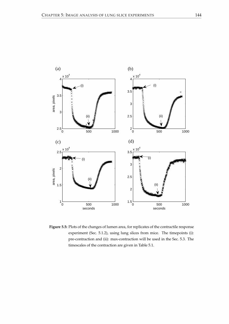
CHAPTER 5: IMAGE ANALYSIS OF LUNG SLICE EXPERIMENTS 144
0 500 10002.5
3
3.5
4x 10
4
area
, pix
els
0 500 10002
2.5
3
3.5
4x 10
4
0 500 10001
1.5
2
2.5x 10
4
seconds
area
, pix
els
0 500 10001.5
2
2.5
3
3.5x 10
4
seconds
(a) (b)
(d)(c)
(i) (i)
(i)(i)
(ii)
(ii)
(ii)
(ii)
Figure 5.5: Plots of the changes of lumen area, for replicates of the contractile response
experiment (Sec. 5.1.2), using lung slices from mice. The timepoints (i):
pre-contraction and (ii): max-contraction will be used in the Sec. 5.3. The
timescales of the contraction are given in Table 5.1.

CHAPTER 5: IMAGE ANALYSIS OF LUNG SLICE EXPERIMENTS 145
150 200 250 300 350 400 450 500 5502.4
2.6
2.8
3
3.2
3.4
3.6x 10
4
time, seconds
area
, pix
els
Figure 5.6: Fitting exponential curves of the form (5.2.1) to the contraction. When two
timescales are used (red) a much better fit is obtained than when just one
timescale is used (blue).
sibilities: either the more complicated model is correct or the simpler model is correct,
but random scattering has led to the more complicated model fitting the data better.
Using the F-distribution (also known as the Fisher-Snedecor distribution) the probabil-
ity that scattering is the cause can be found. MATLAB is used to find the p-value by
subtracting the F cumulative distribution function, which depends on the F-ratio and
the degrees of freedom of the numerator and the denominator of (5.2.2), from one, such
that
p = 1− fcdf (F, DF1 − DF2, DF2) . (5.2.3)
Functions of the form (5.2.1) can similarly be fitted to the other plots of the contracting
airways shown in Fig. 5.5 and test whether two timescales are more appropriate than
one. Results are shown in Table 5.1. In the table, lengths have been nondimesionalised
by the average radius of the ellipse fitted to the lumen in the first frame. The initial
area is thus π. There can be quite large differences in the parameters. For example the
timescales are significantly larger for (d). The ratio of the two timescales, however, is
very similar in each of the experiments. In each of the examples, F À 1 and the p-
value is less than 10−16, which shows that there is overwhelming statistical support to
reject the hypothesis that the simple model with one timescale is sufficiently good and
instead accept the more complex model with two timescales.
We now focus on the experiments on pig lung slices. The results from the lumen area
analysis are shown in Fig. 5.7. Although contraction occurs in all of the airways, it can

CHAPTER 5: IMAGE ANALYSIS OF LUNG SLICE EXPERIMENTS 146
star
ttim
een
dti
me
dura
tion
a 1a 2
τ 1a 3
τ 2F
valu
eτ 2
/τ 1
(a)
174
520
346
2.21
0.56
222
.90.
368
210
742
9.16
(b)
194
560
366
1.96
0.60
129
.20.
582
247
1460
08.
48
(c)
182
540
358
1.90
0.83
132
.80.
416
308
2020
9.40
(d)
126
490
364
1.65
1.16
67.5
0.32
861
799
.89.
14
Tabl
e5.
1:Su
mm
ary
ofm
ouse
resu
lts
show
nin
Fig.
5.5.
τ 1an
dτ 2
are
tim
esca
les
inse
cond
s.a 1
,a2,
and
a 3ar
ear
eas
nond
imes
iona
lised
byth
e
squa
reof
the
radi
usat
the
star
ttim
e.Th
edi
ffer
ence
inti
mes
cale
sτ 2
/τ 1
isfa
irly
cons
iste
ntin
thes
eex
ampl
es.(
b)an
d(c
)are
sepa
rate
airw
ays
from
the
sam
elu
ngsl
ice.
Inea
chof
the
case
the
pva
lue
isle
ssth
an10−1
6 .

CHAPTER 5: IMAGE ANALYSIS OF LUNG SLICE EXPERIMENTS 147
vary a lot from slice to slice. In some slices an initial rapid response is followed by a
sustained slower response, however, in other examples this second timescale is not so
prominent and the graph flattens off. In other examples the airway begins to dilate
again immediately following the initial contraction.
We again now look for evidence of the existence of multiple timescales and if they exist
whether the ratio of the timescales is similar to that with the mice. For the slices that
have an initial rapid contraction followed by a slower contraction, an exponential func-
tion is fitted. A summary of the parameters found are shown in Table 5.2. The start and
end times have been chosen so that the contraction has started and is stopped before
the washout process has an effect. On initial observation there appears to be quite a
bit of variation in the results obtained with fitting the data. There is less variation if
the cases being considered is narrowed to those where the duration is greater than 250s
(highlighted yellow within the table). In this case, for four out of the five experiments,
the ratio of timescales is within a range of two, while the ratio of the fifth is of the same
order of magnitude. The ratio of timescales is reduced in comparison to the results for
the mouse data. Also as with the mouse data, the F ratio is large and for each of the
highlighted cases the p-value is less than 10−16 again indicating overwhelming support
for rejecting the hypothesis that there is only a single timescale. However, there remain
questions about why some of the other airways react like they do.
Finally we consider a few of the experiments of Lavoie et al. [105], that used human
lung slices. Once again in each case there is a rapid contraction on the onset of agonist.
However, the subsequent motion is varied (Fig. 5.8). In one of the plots there is a sus-
tained contraction, while in another the contraction levels off, with a slight relaxation,
while in the third more relaxation is observed. In order to further consider human lung
slices, access to additional experimental data would be needed.
5.2.3 Comparisons to mathematical model
The predictions from the mathematical model described in Sec. 4.2 can be compared
with experimental data. In particular it can be shown that the model predicts multiple
timescales of contraction as shown by the data. First comparisons are made to the
contraction shown in Fig. 5.5 (a). By taking the frame at (i), using the lumen boundary
and an estimation of the outer edge of the airway wall, an estimate for the average
thickness of the airway wall can be calculated, thus we let χ = 0.21. We also set τa = 0,
Rp = 10 and to mimic the parenchyma being fixed far from the airway, as in the lung
slice experiment, we prescribe rp = Rp. β = 3.5 so that at steady state, the percentage
contraction is roughly that of the maximum contraction of the lung slice experiment.

CHAPTER 5: IMAGE ANALYSIS OF LUNG SLICE EXPERIMENTS 148
0 200 400 600 800 10000
5000
10000
0 200 400 600 800 10002000
3000
4000
0 200 400 600 800 10001000
2000
3000
0 200 400 600 800 10000
2000
4000
0 200 400 600 800 10002000
4000
6000
area
, pix
els
0 200 400 600 800 1000
6000
8000
10000
0 200 400 600 800 10003000
4000
5000
0 200 400 600 800 10003000
4000
5000
0 200 400 600 800 10000
2000
4000
0 200 400 600 800 10002000
3000
4000
0 200 400 600 800 10002000
3000
4000
time, seconds
0 200 400 600 800 10000
5000
10000
(f)
(d)
(b)
(j)
(h)
(l)(k)
(i)
(g)
(e)
(a)
(c)
Figure 5.7: Plots of the changes of lumen area, for replicates of the contractile response
experiment (Sec. 5.1.2), using lung slices from pigs. Contraction timescales
are given in Table 5.2.
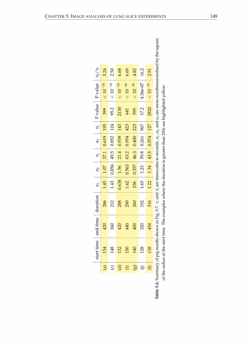
CHAPTER 5: IMAGE ANALYSIS OF LUNG SLICE EXPERIMENTS 149
star
ttim
een
dti
me
dura
tion
a 1a 2
τ 1a 3
τ 2F
valu
eP
valu
eτ 2
/τ 1
(a)
134
420
286
1.45
1.07
37.1
0.61
919
539
9<
10−1
65.
24
(c)
148
360
212
1.43
0.85
649
.50.
852
124
95.2
<10−1
62.
50
(d)
132
420
288
0.63
81.
5621
.40.
939
143
2130
<10−1
66.
68
(f)
150
440
290
1.62
0.56
363
.20.
954
423
641
<10−1
66.
69
(g)
140
400
260
238
0.35
746
.30.
400
223
595
<10−1
64.
82
(j)12
832
019
21.
651.
2359
.80.
261
967
17.2
4.36
e-07
16.2
(l)
138
454
316
1.22
1.34
43.5
0.57
412
728
20<
10−1
62.
91
Tabl
e5.
2:Su
mm
ary
ofpi
gre
sult
ssh
own
inFi
g.5.
7.τ 1
and
τ 2ar
eti
mes
cale
sin
seco
nds.
a 1,a
2,an
da 3
are
area
sno
ndim
esio
nalis
edby
the
squa
re
ofth
era
dius
atth
est
artt
ime.
The
exam
ples
whe
reth
edu
rati
onis
grea
ter
than
250s
are
high
light
edye
llow
.

CHAPTER 5: IMAGE ANALYSIS OF LUNG SLICE EXPERIMENTS 150
0 1000 2000 3000 4000 5000 6000 7000 8000 90000
200
400
600
800
area
, pix
els
0 1000 2000 3000 4000 5000 6000 7000 8000 9000200
400
600
800
1000
1200
area
, pix
els
0 1000 2000 3000 4000 5000 6000 7000 8000 90000
500
1000
1500
time, seconds
area
, pix
els
(i)
(i)
(i)
(ii)
(ii)
(ii)
(iii)
(iii)
(iii)
(a)
(c)
(b)
Figure 5.8: Examples of changes of lumen area, for replicates of the contractile re-
sponse experiment (Sec. 5.1.3) of Lavoie et al. [105] using human lung
slices. The timepoints (i): pre-contraction, (ii): max-contraction and (iii):
end of expiration will be used in Sec. 5.3.

CHAPTER 5: IMAGE ANALYSIS OF LUNG SLICE EXPERIMENTS 151
0 5 10 15 20 25 30 35 400.65
0.7
0.75
0.8
0.85
0.9
0.95
1
Time, s
Nor
mai
lsed
are
a
Figure 5.9: Comparisons are made between the lumen area (crosses) from Fig. 5.5 (a)
and the model prediction (using Sec. 4.2). χ = 0.21, τa = 0, Rp = 10, with
rp = Rp and rates given by Table. 4.2. Predictions when β = 3.5 (blue) or
when g1, g2 and g3 are multiplied by 10 and β = 5 (red).
Initially the airway is assumed to be unstressed and using the rate parameters of HHM,
as given in Table. 4.2, a simulation of the contracting airway is run.
A plot showing the area from the image analysis (crosses) and the model prediction
(blue) are shown in Fig. 5.9. The curve shows evidence of multiple timescales. How-
ever, the initial contraction is too rapid, and then for most of the time the predicted
area is greater than that of the data. It has been suggested that it is more appropriate
to increase the rate of detachment of latch bridges tenfold [173]. Assuming this, we
now choose β = 5, so that at steady state, the percentage contraction is again roughly
that of the maximum contraction of the lung slice experiment. This provides a closer fit
(red) although the initial contraction is still too rapid. These comparisons show that the
model predicts that multiple timescales are associated with the contraction. However,
further analysis of the correct rate parameters is required.
The reason for the multiple timescales is now considered. The active force is related to
the crossbridge distribution as recalling (2.3.17),
A(t; R) = β∫ ∞
−∞x(nC(x, R, t) + nD(x, R, t))dx. (5.2.4)
Recalling (2.3.10),∂n∂t− v
∂n∂x
= Qn, (5.2.5)
the evolution of the crossbridge distribution is affected by the velocity of sliding be-
tween the filaments, v. For now we consider the simpler case when v = 0 and show

CHAPTER 5: IMAGE ANALYSIS OF LUNG SLICE EXPERIMENTS 152
0 5 100
0.2
0.4
0.6
0.8
t
n C+
n D
(a)
0 5 100
0.5
1
t
d(n C
+n D
)/dt
(b)
Figure 5.10: Plots of (a) nC + nD and (b) its derivative against time. Also shown in
(a) are results of fitting the latter part of the curve with one (blue) or two
(red) timescales.
that in this case there is evidence of multiple timescales being associated with the evo-
lution of the total of the attached crossbridges nC + nD. The rate constants for HHM
from [116], as described in Table 4.2, are applied. There is a rapid increase in the num-
ber of of attached crossbridges, before the number levels off (Fig. 5.10 (a)). Considering
the timescales involved, initially the rate of change of nC + nD (Fig. 5.10 (b)) increases
before peaking and then decreasing. This is due to the crossbridges first needing to be
phosphorylated before they can attach. Exponential curves of the form given in (5.2.1)
are fitted to nC + nD after t = 0.5, which is thus after the step change in the value of k1
and k6, which could affect the timescales observed. Fig. 5.10 (a) shows that including
two timescales (red), the fit is very close to the total of the attached crossbridges and
better than the fit with a single timescale (blue). The ratio of the two timescales is 11.1.
Comparing Tables 5.1 and 5.2, in general the ratio of the two timescales related to the
contraction of the airways was larger for the mouse slices than the pig slices. One pos-
sibility for the difference is that the rate parameters, associated with the crossbridge
mechanics, could be species specific. By multiplying the nondimensional rate of at-
tachment of crossbridges by 0.75 and again fitting to a function of the form (5.2.1), the
ratio of the two timescales in the HHM model reduces from 11.1 to 9.7.
This shows that multiple timescales can be explained by the evolution of the distribu-
tion of the crossbridges. However, there are a number of other factors that could also
have an effect. First, rather than the rates of phosphorylation having one value for the
initial 5 seconds and then a lower value thereafter, the value is more time dependent.
During a contraction it is also the case that v 6= 0 and is coupled to the tissue mechanics.

CHAPTER 5: IMAGE ANALYSIS OF LUNG SLICE EXPERIMENTS 153
Recalling (3.1.8),
[[τ]] = log(
raRb
rb
)+
(r2a − 1)(R2
b − 1)2r2
ar2b
+ H(ra − 1)C1
√π
C2cos2 ϕ
(erfi
√C2
(r2
a − 1)
cos2 ϕ− erfi
√C2
(r2
a − 1R2
b
)cos2 ϕ
)
+ 2 cos2 ϕ∫ Rb
1
AR
dR, (5.2.6)
thus for a given transmural pressure, there is a nonlinear relationship between the in-
tegral, which give the contribution of the contractile force over the wall, and the lumen
radius, with the airway stiffening as the airway contracts. This stiffening can affect
the timescales of contraction, by reducing the speed of contraction as the airway nar-
rows. Furthermore, in Chapter 4 the model predicted that the contraction is slower if
the parenchyma is viscoelastic than if it is elastic.
5.3 Displacement analysis and strain fields
Having considered how the lumen area changes during a contraction, the focus shifts
to finding the displacement field for the tissue surrounding the lumen, between two
frames from a video of a lung slice experiment. We introduce two methods that provide
estimates of the displacement field, which we test, and choose the one that is superior.
Using the chosen method, the displacement fields formed when mouse and human
lung slices contract are investigated. In particular, we consider the level of heterogene-
ity and how the displacement varies with distance from the lumen, and compare the
findings to our model predictions.
5.3.1 Methods
In this subsection we present two methods to find an estimate of the displacement
field, which we will test in the following subsection. We base our methods on the work
of Farnebäck [41] and Butler et al. [24]. We also describe a method that enables us to
consider the displacement of sets of points that radiate out from the lumen. Finally we
describe how strain fields can be found from displacement fields.

CHAPTER 5: IMAGE ANALYSIS OF LUNG SLICE EXPERIMENTS 154
5.3.1.1 Farnebäck method
We now introduce the methods used with the Farnebäck algorithm [41]. The algorithm
as implemented in the opencv code cv::calcOpticalFlowFarneback2, which calculates
an estimate of the displacement vector between an initial and final image, for each of
the pixels, was used. In order to make the features in each of the images more promi-
nent, prior to using the algorithm the contrast of each image is increased. Each of the
images is converted to greyscale and the range of the pixel intensities is stretched so
that 1% of the pixels are saturated at the brightest value and 0.01% are saturated at
the darkest value. The following MATLAB commands are used to do this: imread,
rgb2gray, stretchlim, imadjust and imwrite. It is possible that some regions may
remain, where there are not enough features and so insufficient contrast, yielding spu-
rious displacements. Provided that in these regions the pixels are all very light or dark,
thresholds can be set, beyond which the displacements are recalculated by interpolat-
ing. For any such points, the displacement is first set to NAN and then griddata in
MATLAB is used, with the v4 method, to update the displacement each of these points.
In the next few paragraphs we give an overview of the Farnebäck algorithm, follow-
ing [41]. Suppose that the two images are approximated by quadratic polynomial func-
tions that describe the intensity of the pixels at position x. The polynomials for the first
and second image have the form
f1(x) =xTA1x + bT1 x + c1, (5.3.1)
f2(x) =xTA2x + bT2 x + c2, (5.3.2)
where A1, A2 are matrices, b1, b2 are vectors and c1, c2 are scalars. If the two images are
only different by a rigid shift, f1(x) = f2((x− d)), where d is the displacement of the
shift to be found. In this case
A2 = A1, b2 = b1 − 2A1d, c2 = dTA1d− bT1 d + c1, (5.3.3)
where, assuming that A1 is non-singular, d is given by
d = −A1b2 − b1
2. (5.3.4)
In general it is more complicated than this, since the displacement is spatially depen-
dent and will also involve rotation and stretching. Rather than finding intensity poly-
nomial functions over the whole region, local polynomial functions are found over a
small neighbourhood surrounding each of the pixels. A spatially-dependent displace-
ment d(x) is found using the local polynomials of the two images. If however, the
2http://opencv.willowgarage.com/documentation/cpp/motion_analysis_and_object_tracking.html

CHAPTER 5: IMAGE ANALYSIS OF LUNG SLICE EXPERIMENTS 155
displacements are large, the comparison of local polynomials in the two images may
be insufficient, since the displaced point may not be located within the local neighbour-
hood of the initial position used to form the polynomial. In this case a false displace-
ment will be found. The algorithm is able to overcome this problem by using a priori
knowledge. Given an a priori displacement d(x), a relative displacement can be found
using f1(x) and f2(x), where x = x + d(x). d(x) (which is measured relative to pixel
width) is rounded to the nearest integer, so that the polynomial in the second image is
centred on a pixel. Now in general, A1 6= A2, but introducing
A(x) =A1(x) + A2(x)
2, ∆b(x) = −1
2(b2(x)− b1(x)) + A(x)d(x), (5.3.5)
the constraint for the updated displacement is
A(x)d(x) = ∆b(x). (5.3.6)
In practice the displacement field that is found will be too noisy. The algorithm over-
comes this by assuming that the displacement field is only slowly varying. In this case,
for each pixel, it is possible to solve with an appropriate weight function w(∆x) over
a region Ω, which forms a square of pixels around the current pixel. This results in
having to find the minimum of
∑∆x∈Ω
w(∆x)‖A(x + ∆x)d(x)− b(x + ∆x)‖2. (5.3.7)
Increasing the size of Ω results in smoother displacement fields.
In reality an initial guess of the displacements is generally not available, in which case
an iterative system can be used. The initial iterations are used to find an approximation
of the displacements, with further iterations improving the approximation. If the dis-
placement between the two frames is large, the initial size of the neighbourhood, used
to fit the polynomials f1(x) and f2(x), can be increased, in order to find a rough but
reasonable displacement estimation. This displacement can then be used as the a priori
displacement, which can be improved in two ways. Further iterations can be carried
out with the same neighbourhood size, or in order to find more of the local features
of the displacement field, the size of the neighbourhood of the pixels used to find the
polynomials can be reduced.
When implementing the opencv code, unless otherwise stated we use three sizes of
square neighbourhoods to form the pixel intensity polynomials. For each subsequent
square size we halve the length of sides and iterate three times for each size. Using the
suggested values in the opencv documentation, we use a final side length of 5 pixels
and set the standard deviation of the Gaussian, used to smooth derivatives in order to

CHAPTER 5: IMAGE ANALYSIS OF LUNG SLICE EXPERIMENTS 156
form the polynomials f1(x) and f2(x), as 1.1 pixels. We find that introducing additional
larger squares does not improve the results.
5.3.1.2 Butler method
The algorithm of Butler et al. [24] was developed to track fluorescent beads on a con-
tracting gel, estimating a sparse displacement field between two images. We adapt this
algorithm to track features of the lung slice. In comparison to the fluorescent beads,
since the lung slices are lit from behind, the brightest areas are regions where there is
no tissue. Prior to using the algorithm, we take the complement of the original images,
so that the tissue is light and the background is dark. For the rest of this subsection we
give an overview of the code of Butler et al. [24].
There are a number of similarities between the Butler et al. [24] and Farnebäck [41] al-
gorithms. Functions describing the intensities of squares of pixels in the two images
are compared to find the shift in the second image that yields the best match. To over-
come issues with large displacements, larger regions of pixels are first compared before
reducing the number of pixels that are compared to acquire more of the local subtleties.
The algorithm of Butler et al. [24] consists of splitting the two images into a number of
squares. Cross-correlation is used to compare a square in the first image to the corre-
sponding square in the second image and find the coordinates of the shift of the second
square so that the two squares have the highest correspondence. Functions f (x, y), for
a square of pixels in the first image, and g(x, y), for the corresponding square of pixels
in the second image, describe the pixel intensities for each of the coordinates (x, y). By
definition [16, 180] the cross-correlation of the two functions is
( f ? g)(x, y) ≡∞
∑u,v=−∞
f ∗(u, v)g(u + x, v + y), (5.3.8)
where f ∗ is the complex conjugate of the function f . Since the intensity is a real value,
the complex conjugate is equal to the original value. The largest value of (5.3.8) indi-
cates the best correspondence. Taking Fourier transforms of each side of (5.3.8) yields
F ( f ? g) = FG, (5.3.9)
where F is the complex conjugate of the Fourier transform of the function f and G is
the Fourier transform of the function g. Due to the possibility of light intensity changes
between the two images, the Fourier transforms of the two images can be normalised.
They are normalised by dividing the two functions by the maximum value of the cor-
relation of the whole image with itself. The fast Fourier transform of a square of pixels

CHAPTER 5: IMAGE ANALYSIS OF LUNG SLICE EXPERIMENTS 157
d
(a) (b)
2 resres
2 2 r
es
Figure 5.11: (a) Each of the two images are split up into squares. Once a good approx-
imation of the displacement has been found, each of the squares is split
into four smaller squares. The smaller squares of pixels are then used
to carry out the cross-correlation to fine-tune the displacement. This is
repeated until the distance between the mid points of adjacent squares
equals the required resolution (res). (b) Having found an approximation
for the displacement, this displacement is used to alter the coordinates of
the square in the second image. Cross-correlation can then be repeated to
fine-tune the displacement.
can be calculated using the MATLAB function fft2(x), the complex conjugate, using
conj(x) and the inverse fast Fourier transform, using ifft2(x).
Due to the possibility of large displacements, the algorithm includes a number of it-
erations over squares of reducing size. An initial size, whose choice is limited by the
dimensions of the image, is chosen to find a rough estimate of the displacement field,
which can be used to select the location of the squares in the second image. Having
found a reasonable estimate of the displacement, the width of the square is halved
(Fig. 5.11 (a)) and the displacements are fine tuned. This is repeated until the size of
the squares matches the resolution required. For each size of square, a number of steps
are carried out. Having split up the image into squares, for each of the squares the nor-
malised cross-correlation with the corresponding square in the second image is found.
The maximum correlation gives the displacement required of the second square. The
square in the second image is shifted by this current estimation of the displacement
(Fig. 5.11 (b)), and the cross-correlation step is repeated in order to fine tune the dis-
placement. These two steps are repeated until there is no additional displacement or a
maximum number of steps have been taken.
After the final iteration with a given square size, a number of checks are carried out. If

CHAPTER 5: IMAGE ANALYSIS OF LUNG SLICE EXPERIMENTS 158
for any of the points any of the following do not hold, the point is declared as being
unreliable and the displacement at that point is set to NAN:
• the latest change in the displacement was not zero, indicating the squares are not
best aligned;
• the latest change in the displacement in the x or y direction is greater than half of
the current size of the squares, indicating too much displacement at this level;
• the maximum pixel intensity is below some minimum value, indicating that the
square consisted of data for the background but not the tissue;
• the maximum correlation is below a threshold.
In order to improve the displacement by comparing smaller squares, every square is
split into four smaller squares and the new coordinates of the centre of the squares in
the first image are calculated. Estimates of the displacements at each of these points are
found by fitting a smooth surface to the old accepted displacements. The estimates of
the displacements are used to choose the starting positions of the squares in the second
image. Following the final level, a surface is fitted to approximate for points where the
displacement was rejected.
5.3.1.3 Finding displacements for points along normal vectors
An alternative to finding the displacement field is to find the displacement at selected
points. By selecting points along a normal vector to the lumen, it is easy to show how
the displacement changes with radius. By doing likewise at various points around
the lumen the displacement-radius relationship at each can be compared. We split the
airway into eight sections, within each of which we select points along normal vectors
that begin at seven points on the lumen boundary. We solve to find displacements
in the tangential and normal directions, averaging the predictions within each of the
sections for each radial position, to try to remove any small errors. As it is expected
that there will be little variation in each of the sections, checks can be made that the
standard deviation is small.
We begin by fitting an ellipse to the lumen at the start of the contraction, using the
techniques described in section 5.2.1. In parametric form an ellipse centred at (x0, y0),
with major and minor axis of length 2a and 2b and angle α between the x axis and the

CHAPTER 5: IMAGE ANALYSIS OF LUNG SLICE EXPERIMENTS 159
major axis, has coordinates
x = x0 + a cos t cos α− b sin t sin α, (5.3.10a)
y = y0 + a cos t sin α + b sin t cos α, (5.3.10b)
where t ∈ [0, 2π) is the parametric parameter. The unit vectors in the tangential and
normal directions are
t =(−a sin t cos α− b cos t sin α,−a sin t sin α + b cos t cos α)√
a2 sin2 t + b2 cos2 t, (5.3.11a)
n =(−a sin t sin α + b cos t cos α, a sin t cos α + b cos t sin α)√
a2 sin2 t + b2 cos2 t. (5.3.11b)
We now explain how the points are chosen. Eight groups of seven points are chosen on
the ellipse with the coordinates
(xe, ye) = (x(t), y(t)) , t = α + mπ/4 + nπ/180, (5.3.12)
with m = 0, 1, .., 7 and n = −3,−2, .., 3. If the ellipse was a perfect fit to the lumen each
of the points would be located at the lumen boundary. In practice the lumen is not so
regular, so the choice of points given in (5.3.12) may need to be slightly altered. Where
required, we slightly inflate or deflate the ellipse, while fixing the ratio of a and b, in
order to select a point on the boundary. For each of the new points we find the normal
to the lumen and select further points spaced by k pixels in the direction of the normal.
This yields the points
(x, y) = (xe, ye) + n(t)ks, s = 0, 1, .... (5.3.13)
An illustration of how one line of points are chosen and an example of the points chosen
is shown in Fig. 5.12. Since in general the coordinates are not integer values, bilinear
interpolation of the four nearest pixels is used to find the displacement. The radial and
azimuthal components of the displacements are found by taking the dot product of the
displacement with the unit normal and tangent vectors.
5.3.1.4 From displacement fields to strain fields
An alternative to plotting displacement fields is to plot strain fields. An advantage
of strains over displacements is that, if there is a rigid displacement of a lung slice
that is not related to the contraction of the airway, while the displacement field will be
affected, the strain field will not. Below we describe the theory that enables the strain
field to be found from the displacement field. In the results section (Sec. 5.3.3), plots
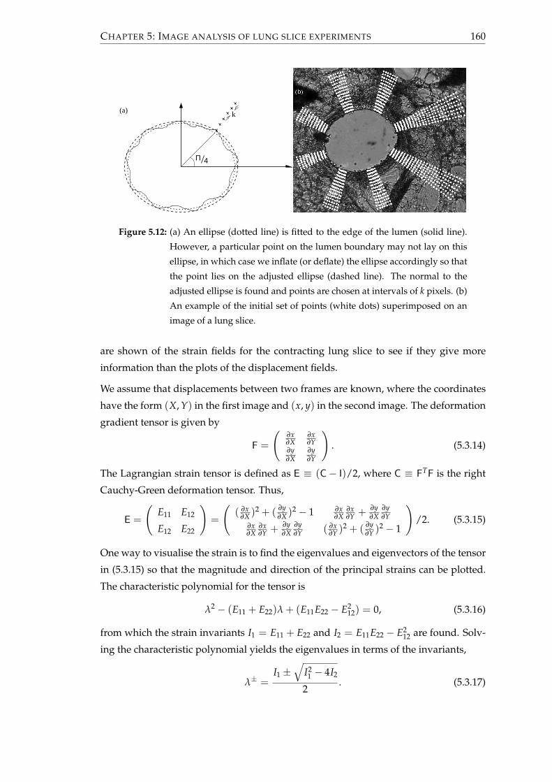
CHAPTER 5: IMAGE ANALYSIS OF LUNG SLICE EXPERIMENTS 160
4Π
k(a)
Figure 5.12: (a) An ellipse (dotted line) is fitted to the edge of the lumen (solid line).
However, a particular point on the lumen boundary may not lay on this
ellipse, in which case we inflate (or deflate) the ellipse accordingly so that
the point lies on the adjusted ellipse (dashed line). The normal to the
adjusted ellipse is found and points are chosen at intervals of k pixels. (b)
An example of the initial set of points (white dots) superimposed on an
image of a lung slice.
are shown of the strain fields for the contracting lung slice to see if they give more
information than the plots of the displacement fields.
We assume that displacements between two frames are known, where the coordinates
have the form (X, Y) in the first image and (x, y) in the second image. The deformation
gradient tensor is given by
F =
(∂x∂X
∂x∂Y
∂y∂X
∂y∂Y
). (5.3.14)
The Lagrangian strain tensor is defined as E ≡ (C− I)/2, where C ≡ FTF is the right
Cauchy-Green deformation tensor. Thus,
E =
(E11 E12
E12 E22
)=
(( ∂x
∂X )2 + ( ∂y∂X )2 − 1 ∂x
∂X∂x∂Y + ∂y
∂X∂y∂Y
∂x∂X
∂x∂Y + ∂y
∂X∂y∂Y ( ∂x
∂Y )2 + ( ∂y∂Y )2 − 1
)/2. (5.3.15)
One way to visualise the strain is to find the eigenvalues and eigenvectors of the tensor
in (5.3.15) so that the magnitude and direction of the principal strains can be plotted.
The characteristic polynomial for the tensor is
λ2 − (E11 + E22)λ + (E11E22 − E212) = 0, (5.3.16)
from which the strain invariants I1 = E11 + E22 and I2 = E11E22 − E212 are found. Solv-
ing the characteristic polynomial yields the eigenvalues in terms of the invariants,
λ± =I1 ±
√I21 − 4I2
2. (5.3.17)

CHAPTER 5: IMAGE ANALYSIS OF LUNG SLICE EXPERIMENTS 161
The eigenvalues depend on a combination of the invariants and so are independent of
the coordinate system used. Now
I21 − 4I2 = (E11 − E22)2 + 4E2
12 ≥ 0, (5.3.18)
so in general there are two real eigenvalues. The only exception is when the tensor is
symmetric and the diagonal elements are equal, for which there is a repeated eigen-
value.
To find the eigenvectors the following equation must be solved:(
E11 − λ± E12
E12 E22 − λ±
) (x
y
)=
(0
0
). (5.3.19)
From the first row, the unit eigenvectors satisfy
(E12, λ± − E11)√E2
12 + (λ± − E11)2.
The second row provides an equivalent relationship. The eigenvalue could equally
point in the opposite direction. We assume that for a single contracted airway, a com-
ponent of the major principal strain will point towards, rather than away from, the
lumen.
5.3.2 Testing the codes
We have presented two different approaches for estimation of the displacements from
one image to another. In this subsection we present two tests to find out how well they
perform. The first test is used to see how well the tissue, in general, is tracked, while
the second test is used to see how well the lumen radius is tracked.
• Test 1: A single lung slice image is taken and is cropped in two different ways, so
one is a uniform rigid shift of the other. The coordinates of the rigid shift in pixels
are (5,7) for the mouse example and (3,4) for the human example. A smaller shift
is chosen for the human slice since the lumen takes up less of the image and the
displacements are in general smaller in terms of pixel number. Each algorithm is
used to predict the displacement from one of the images to the other, which are
subtracted from the imposed displacement to yield an error. Vectors showing the
size of the errors are superimposed on to the first of the images, to show where
errors occur. Near the edge of the image features may be in one of the images but
not the other, due to the nature of the cropping. The errors are thus set to zero
near the edge of the image and within the lumen, where there is no tissue.

CHAPTER 5: IMAGE ANALYSIS OF LUNG SLICE EXPERIMENTS 162
• Test 2: Each of the algorithms is used to estimate the displacement field between
the frame just before contraction starts and the frame of maximum contraction.
Using the techniques described in the section 5.2.1 the edge of the lumen in the
two frames is found and for the points within the lumen the displacement is set to
zero. By plotting the lumen outline for each of the frames and the displacement
vectors, it is possible to establish whether or not each of the algorithms provide a
good approximation of the displacement at the lumen boundary.
We now proceed to use these tests, firstly on frames from experiments that use lung
slices from mice and then from those using lung slices from humans. We do not con-
sider lung slices from pigs, since due to the added thickness of the slices the tissue is
very dark with insufficient contrast.
5.3.2.1 Testing for the mouse slices
Firstly, test 1 is applied to the Farnebäck method (Sec. 5.3.1.1). The importance of in-
cluding the steps to increase the contrast in the images prior to estimating the displace-
ment field and to interpolate over regions where the contrast remains small is shown in
Fig. 5.13. The errors given by the displacement predicted by the algorithm minus the
imposed displacement are plotted at every eight pixels, leaving a gap of twelve pixels
around the edge of the image to account for the image cropping. If the contrast is not
altered, but the original images are used, there is generally good agreement with small
errors, however, there are some regions with large errors (a). The errors are observed
in regions where the pixels are all dark, with little variation. Including the step to alter
the contrast, so that the full range of available pixel intensities is used, there are only a
couple of small (black) regions with large errors (b). If the interpolation step is included
these errors are greatly reduced (c). In this example this algorithm is able to accurately
predict the displacement across the slice.
Secondly, test 1 is applied to the Butler method (Sec. 5.3.1.1). The error, representing
the difference between the estimated value of the displacement and the prescribed rigid
shift, is shown in Fig. 5.14 for two cases. Using the Butler method, initially the image is
split into squares of width 32 pixels, with iterations being carried out until the squares
have a width of 8 pixels. In this case there are some errors, especially around the edge
of the black object in the top left hand corner of the image (a). Doubling the initial
width of the squares, greatly reduces many, but not all, of these errors (b). Increasing
the width of the initial squares further may lead to further reductions in the errors.
However, since the dimensions of the image analysed must be multiples of the width

CHAPTER 5: IMAGE ANALYSIS OF LUNG SLICE EXPERIMENTS 163
(a)
(b)
(c)
Figure 5.13: Plots of the errors (red arrows), representing the displacement predicted
by the Farnebäck method (Sec. 5.3.1.1) minus the imposed displacement,
when using test 1 on a mouse slice. The same scale is used for the arrows
in each of the images. In (a) neither of the steps to alter the contrast of the
images or to interpolate over regions where the contrast remains small
are included. In (b) the step to alter the contrast of the images is included.
In (c) both the steps to alter the contrast of the images and to interpolate
over regions where the contrast remains small are included.

CHAPTER 5: IMAGE ANALYSIS OF LUNG SLICE EXPERIMENTS 164
(a) (b)
Figure 5.14: Plots of the errors (red arrows), representing the displacement predicted
by the Butler method (Sec. 5.3.1.2) minus the imposed displacement,
when using test 1 on a mouse slice. The same scale is used for the ar-
rows in the two images. Initially the image is split into squares of width
(a) 32 pixels or (b) 64 pixels. In both cases the final resolution is 8 pixels.
of the initial square size, this limits the values that can be chosen.
Thirdly, test 2 is applied to an example mouse slice when using the two algorithms.
The lumen edges pre- and post-contraction and the estimated displacement vectors
are shown in Fig. 5.15. Comparing the contour plots of the magnitude of the estimated
displacements in (b, d), in general the two methods predict similar sized displacements.
However, there are some notable differences, especially at the lower left-hand section
of the lumen boundary. In (a, c) the arrows, indicating the predicted displacements,
should point from the outer to the inner red line, which indicate the lumen boundary
pre- and post-contraction. Using the Farnebäck method (a), the arrows provide a good
estimate, whereas with the Butler method the arrows do not point from the outer to
the inner line, indicating errors (c). If the initial size of the squares used in the Butler
method is increased, these problems are not resolved (not shown). In this instance it
can therefore be concluded that the Farnebäck method is superior.
5.3.2.2 Testing for the human slices
We now concentrate on the human lung slices and again test the two methods. There
are a couple of ways in which these slices are different from those from mice; the frac-
tion of the image taken up by the lumen is smaller and there are more gaps in the tissue
surrounding the lumen.
Firstly, test 1 is applied to the Farnebäck method (Sec. 5.3.1.1). In Fig. 5.16 the error,
given by the displacement predicted by the algorithm minus the imposed displace-
ment, is shown. An interpolation step was included into the Farnebäck method, to

CHAPTER 5: IMAGE ANALYSIS OF LUNG SLICE EXPERIMENTS 165
(a)
pixe
ls
100 200 300 400 500
100
200
300
400
0
5
10
15(b)
(c)
pixe
ls
100 200 300 400 500
100
200
300
400
0
5
10
15(d)
Figure 5.15: Test 2 with mouse slices. Plots of (a, c) the estimated displacement vec-
tors (red arrows) and the outline of the lumen pre- and post-contraction
(red lines), and (b, d) the magnitude of the estimated displacements. The
Farnebäck method (Sec. 5.3.1.1) is used in (a, b) and the Butler method
(Sec. 5.3.1.2) is used in (c, d).

CHAPTER 5: IMAGE ANALYSIS OF LUNG SLICE EXPERIMENTS 166
(a) (b)
Figure 5.16: Plots of the errors (red arrows), representing the displacement predicted
by the Farnebäck method (Sec. 5.3.1.1) minus the imposed displacement,
when using test 1 on a human slice. The same scale is used for the arrows
in the two images. Errors when the final interpolation step of the method
is (a) included or (b) not included.
take account of areas where there are no features to track. In the case of the human
lung slices the gaps in the parenchyma are example regions of this. If the interpolation
step is not included then errors are shown in the gaps (a), while including the interpo-
lation step, the errors are greatly reduced (b) and the method provides a good estimate
of the displacements.
Secondly, test 1 is applied to the Butler method (Sec. 5.3.1.1). The error, representing
the difference between the estimated value of the displacement and the prescribed rigid
shift, is shown in Fig. 5.17 for three cases. If initially the image is split into squares of
width 32 pixels and iterations are carried out until there are squares of width 16 pixels,
there are a few points within the airway wall where the deformation is not detected
and errors are shown (a). Doubling the width of the initial square greatly reduces
these errors (b). The final size of the squares can be halved to give estimates of the
displacement at a finer resolution (c).
Thirdly, test 2 is applied to an example human slice using the two algorithms. The
lumen edges pre- and post-contraction and the estimated displacement vectors are
shown in Fig. 5.18. The estimated displacements from the Farnebäck method track
the boundary well, showing small arrows near the top of the lumen where there is lit-
tle change and larger arrows at the bottom where the lumen boundary moves further
(a). In contrast the estimated displacements from the Butler method do not track the
boundary well (b). This is particularly noticeable on the left hand side of the lumen. In
the example shown the starting and final widths of the squares used are 64 and 8 pix-

CHAPTER 5: IMAGE ANALYSIS OF LUNG SLICE EXPERIMENTS 167
(a) (b)
(c)
Figure 5.17: Plots of the errors (red arrows), representing the displacement predicted
by the Butler method (Sec. 5.3.1.2) minus the imposed displacement,
when using test 1 on a human slice. The same scale is used for the ar-
rows in each of the images. Initially the image is split into squares of
width (a) 32 pixels or (b, c) 64 pixels, with the final resolution equal to (a,
b) 16 pixels or (c) 8 pixels.

CHAPTER 5: IMAGE ANALYSIS OF LUNG SLICE EXPERIMENTS 168
(a)(b)
Figure 5.18: Test 2 with human slices. Plots of the estimated displacements (red ar-
rows) when using (a) the Farnebäck method (Sec. 5.3.1.1) or (b) the Butler
method (Sec. 5.3.1.2). The blue lines in the indicate the outline of the lu-
men pre- and post-contraction.
els. Doubling or halving the initial blocksize or increasing the final blocksize is found
not to improve the tracking of the boundary (not shown).
Having carried out the two different tests on both the mouse and human slices, the
Farnebäck method has proved to be superior. In particular it is better at tracking the
lumen boundary. In the following results section the Farnebäck method is used to
estimate the displacement field.
5.3.3 Results
In this subsection the Farnebäck method is used to consider the displacements in the
tissue surrounding an airway. Firstly the displacement fields in three lung slice exper-
iments with contracting mouse airways are considered (Fig. 5.19). For the first slice
(a, b) there are much smaller displacements in the bottom-right section of the image.
In this region of the image of the lung slice there is a thick black diagonal strip. This
is likely to be an arteriole, that may already have collapsed affecting this region and
inhibiting further contraction. Similarly, for the second slice (c, d) the displacements
are smaller in the bottom half of the slice. Again there is a large dark region that could
be affecting the ability of the tissue to contract here. An interesting feature of this slice
is that there are two airways present. In the top half of the slice the displacements are
largely symmetric. With the third slice (e, f) there are some issues in the region above
the lumen. Here there is very little contrast between the tissue and the lumen itself.
These issues have been improved a little by increasing the number of iterations car-
ried out for each successive size of neighbourhood, used to fit a polynomial function to

CHAPTER 5: IMAGE ANALYSIS OF LUNG SLICE EXPERIMENTS 169
the pixel intensities, from three to five. While there are some regions where there are
reduced displacements or where the displacements are not picked up, in general the
largest displacements in each example are seen at the lumen boundary. With distance
from the lumen, the magnitude of the displacement initially rapidly reduces before
starting to level off.
In Sec. 5.3.1.4 the theory required to find Lagrange strain tensor from the displacement
field was presented. The size and direction of the principal strains can be found by
finding eigenvalues and vectors. Using this theory, plots of the major and minor strains
are shown in Fig. 5.20 for the first two examples shown in Fig. 5.19. The white lines
show that the major principal strain is predominantly in the radial direction. Except for
a few small regions, the major principal strains are positive indicating radial stretching.
The minor principal strains are perpendicular to those of the major principal strains so
are predominantly in the circumferential direction. Except for a few small regions, the
minor principal strains are negative indicating compression. For the slice with two
airways (c, d), there is a region between the two airways where the major and minor
eigenvalues are quite large. This is due to this region experiencing biaxial tension as
both of the airways contract. A disadvantage of these plots is that they are quite noisy,
since any noise from the displacement field will be emphasised when finite difference
schemes are used to find the strain.
In Sec. 5.3.1.3 we showed how, rather than simply finding the displacement field, we
are able to find the displacement at selected points. By selecting points along spokes ra-
diating out of the lumen, we are able to give further consideration to the heterogeneity
of the airway and can find the size of the components of the displacement in the ra-
dial and circumferential directions. Slice (a) from Fig. 5.19 is used and the initial points
are shown in Fig. 5.21 (a). For the initial time point, the time just prior to the start of
contraction is used. Four further points are chosen (b), for which the slice experiences
increasing amounts of contraction, and the displacement, relative to the frame at the
initial time point, is found at each of these times. Taking each section in turn, the aver-
age radial component of the displacement is plotted for each of the radial positions and
time points (c-j). Within each of the sections there is little variation, as shown by the
small error bars. Considering the shape of the radius-displacement curves, the largest
displacement is generally seen at the lumen boundary (R = 1). For a number of the
sections, close to the lumen the gradient of the curves is quite steep, before levelling
off as R increases. There are also similar shapes at the four time points. Comparing the
different regions, however, there is significant heterogeneity.
The extent of heterogeneity in the tissue surrounding an airway can be further investi-

CHAPTER 5: IMAGE ANALYSIS OF LUNG SLICE EXPERIMENTS 170
(a)
100 200 300 400 500
50
100
150
200
250
300
350
400
450
0.05
0.1
0.15
0.2(b)
(c)
100 200 300 400 500 600
50
100
150
200
250
300
350
400
450
0
0.05
0.1
0.15
0.2
0.25
0.3
(d)
(e)
100 200 300 400 500 600
50
100
150
200
250
300
350
400
450
0.05
0.1
0.15
0.2
0.25
(f)
Figure 5.19: Three examples of the displacement fields in contracting mouse lung-
slices. Plots of (a, c, e) the estimated displacement vectors and the lu-
men boundary pre- and post-contraction and (b, d, f) the corresponding
displacement magnitudes. (The magnitudes have been normalised by di-
viding through by the average radius of the lumen.) The initial and final
time points are labelled (i) and (ii) in Fig. 5.5, with (a, b), (c, d) and (e, f)
showing respectively the airways labelled (a), (b, c) and (d) in Fig. 5.5.

CHAPTER 5: IMAGE ANALYSIS OF LUNG SLICE EXPERIMENTS 171
100
200
300
400
500
50100
150
200
250
300
350
400
450
−0.
2
00.2
0.4
0.6
(a)
100
200
300
400
500
50100
150
200
250
300
350
400
450
−0.
4
−0.
3
−0.
2
−0.
1
00.1
(b)
100
200
300
400
500
600
50100
150
200
250
300
350
400
450
−0.
2
00.2
0.4
0.6
0.8
1(c
)
100
200
300
400
500
600
50100
150
200
250
300
350
400
450
−0.
5
−0.
4
−0.
3
−0.
2
−0.
1
00.1
0.2
0.3
(d)
Figu
re5.
20:P
lots
of(a
,c)
the
maj
orei
genv
alue
sof
the
Lagr
ange
stra
inte
nsor
(wit
har
row
ssh
owin
gdi
rect
ion
ofei
genv
ecto
rs)
and
(b,d
)th
e
min
orei
genv
alue
s(v
ecto
rsar
epe
rpen
dicu
lar
toth
ose
ofth
em
ajor
eige
nvec
tors
).Th
ese
stra
ins
in(a
,c)
and
(b,
d)co
rres
pond
resp
ecti
vely
toth
eai
rway
ssh
own
in(a
,c)a
nd(b
,d)i
nFi
g.5.
19.
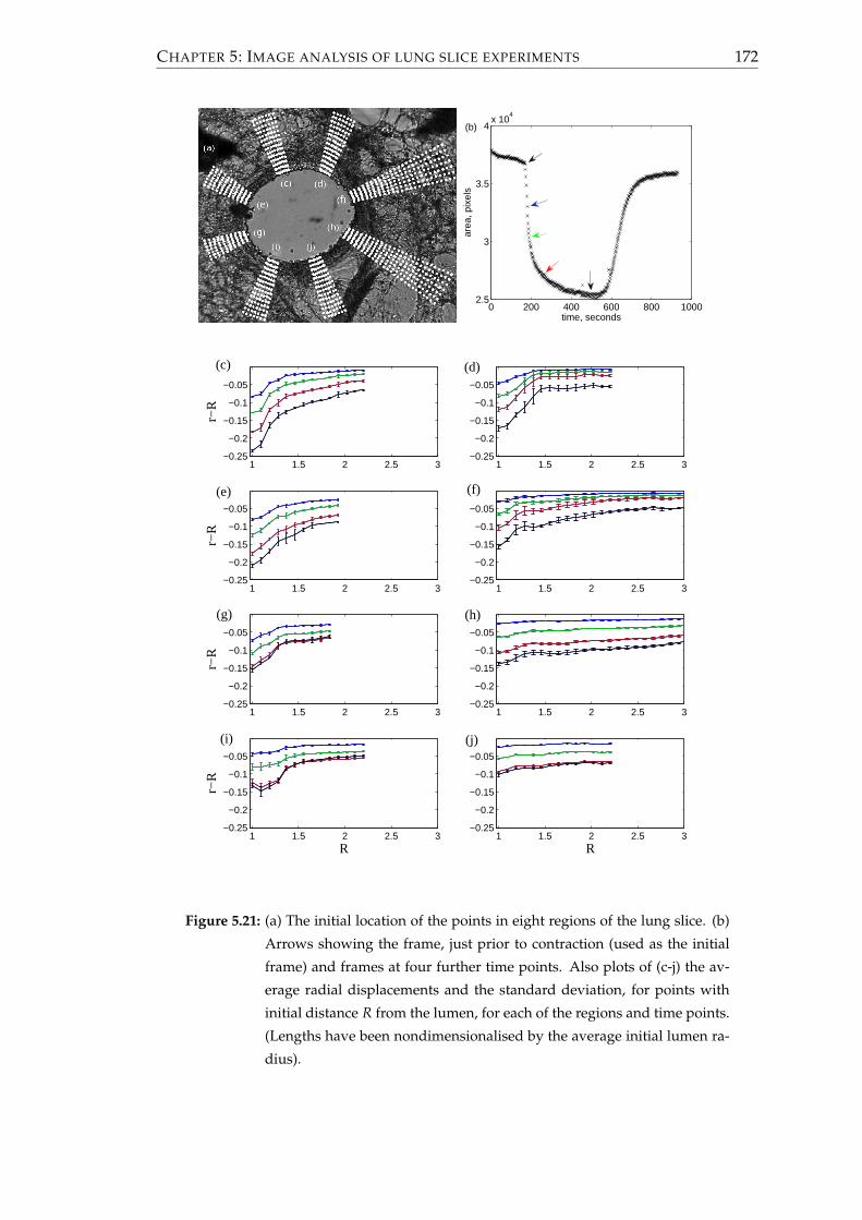
CHAPTER 5: IMAGE ANALYSIS OF LUNG SLICE EXPERIMENTS 172
0 200 400 600 800 10002.5
3
3.5
4x 10
4
time, seconds
area
, pix
els
(b)
1 1.5 2 2.5 3−0.25
−0.2
−0.15
−0.1
−0.05
1 1.5 2 2.5 3−0.25
−0.2
−0.15
−0.1
−0.05
1 1.5 2 2.5 3−0.25
−0.2
−0.15
−0.1
−0.05
r−R
1 1.5 2 2.5 3−0.25
−0.2
−0.15
−0.1
−0.05
r−R
1 1.5 2 2.5 3−0.25
−0.2
−0.15
−0.1
−0.05
r−R
1 1.5 2 2.5 3−0.25
−0.2
−0.15
−0.1
−0.05
R
r−R
1 1.5 2 2.5 3−0.25
−0.2
−0.15
−0.1
−0.05
R
1 1.5 2 2.5 3−0.25
−0.2
−0.15
−0.1
−0.05
(c) (d)
(f)
(h)
(j)(i)
(g)
(e)
Figure 5.21: (a) The initial location of the points in eight regions of the lung slice. (b)
Arrows showing the frame, just prior to contraction (used as the initial
frame) and frames at four further time points. Also plots of (c-j) the av-
erage radial displacements and the standard deviation, for points with
initial distance R from the lumen, for each of the regions and time points.
(Lengths have been nondimensionalised by the average initial lumen ra-
dius).

CHAPTER 5: IMAGE ANALYSIS OF LUNG SLICE EXPERIMENTS 173
1 1.2 1.4 1.6 1.8
−0.2
−0.15
−0.1
−0.05
0
R
r−R
Figure 5.22: Plot showing the average radial displacements and standard deviation
when averaging over all the spokes in Fig. 5.21.
gated, if instead of averaging within each of the sections separately, an average is taken
over all of the sections together. The resulting averages of the radial components of the
displacement are shown in Fig. 5.22. Again on average the largest displacements are
found at the lumen. Now there are large error bars indicating a lot of variation in the
radial displacements, whereas when averaging within each of the sections individually
the error bars were small (Fig. 5.21).
Having considered the component of the displacement in the radial direction, the com-
ponent in the circumferential direction is considered. Averaging within each of the
sections, the standard deviations are generally very small (Fig. 5.23). In comparison to
the results for the radial component, the displacements are much smaller and do not
necessarily increase with time. Comparing the distributions of the displacement in the
different sections, there is no one fixed shape. At some points the displacement is in
the positive direction, while at other points it is in the negative direction. This can be
explained by the fact that the shape of the airway and the distribution of the smooth
muscle is non-axisymmetric.
Having considered the displacement fields for various mouse lung slices, we consider
some examples for human lung slices. In particular we use the lung slice experiments
of Lavoie et al. [105], for which the lumen-area timecourses were shown in Fig. 5.8. As
described in Sec. 5.1.3, the experiment consisted of ten minutes for the airway to con-
tract following the addition of MCh, ten minutes where tidal oscillations were applied
to the parenchyma and ten further minutes with no oscillations. Three timepoints were
indicated in Fig. 5.8, that were situated (i) just prior to contraction, (ii) by the maximum
contaction and (iii) following the application of oscillations in the parenchymal strain.

CHAPTER 5: IMAGE ANALYSIS OF LUNG SLICE EXPERIMENTS 174
0 200 400 600 800 10002.5
3
3.5
4x 10
4
time, seconds
area
, pix
els
(b)
1 1.5 2 2.5 3−0.1
−0.05
0
0.05
0.1
1 1.5 2 2.5 3−0.1
−0.05
0
0.05
0.1
1 1.5 2 2.5 3−0.1
−0.05
0
0.05
0.1
u θ
1 1.5 2 2.5 3−0.1
−0.05
0
0.05
0.1
u θ
1 1.5 2 2.5 3−0.1
−0.05
0
0.05
0.1
u θ
1 1.5 2 2.5 3−0.1
−0.05
0
0.05
0.1
R
u θ
1 1.5 2 2.5 3−0.1
−0.05
0
0.05
0.1
R
1 1.5 2 2.5 3−0.1
−0.05
0
0.05
0.1
(c) (d)
(e) (f)
(g) (h)
(i) (j)
Figure 5.23: (a, b) as in Fig. 5.21. Also plots of (c-j) the average circumferential dis-
placements and the standard deviation, for points with initial distance R
from the lumen, for each of the regions and time points. (Lengths have
been nondimensionalised by the average initial lumen radius).

CHAPTER 5: IMAGE ANALYSIS OF LUNG SLICE EXPERIMENTS 175
Results will now be shown for displacements from (i) to (ii) and then from (i) to (iii).
Plots showing the displacements from (i) prior to contraction to (ii) maximal contrac-
tion are shown in Fig. 5.24. Again there is strong evidence of heterogeneity. Where
there is more tissue, rather than gaps, there are larger displacements. So for example
in slice (a) there is a thick piece of tissue that protrudes from the bottom-right section
of the wall into the parenchyma. In this region there is clear evidence of increased dis-
placement. Similarly to the results for mice airways, the magnitude of the displacement
decreases with distance from the lumen.
Plots showing the displacements from (i) prior to contraction to (iii) after the appli-
cation of oscillations, as described in Sec. 5.1.3, are shown in Fig. 5.25. The strain os-
cillations result in reduced displacements in comparison to those shown in Fig. 5.24,
although in general the regions of the slice with larger or smaller than average displace-
ments are the same. Again the magnitude of the displacement generally decreases as
the distance from the lumen increases.
5.3.4 Comparisons to the mathematical model
In this subsection, we make some comparison between the model predictions and ex-
perimental data. The model presented in the previous chapters assumes plane strain,
while for an intact airway plane stress may be more appropriate. Using the model of
Brook et al. [22] we make comparisons between the two approaches. Ensuring that the
outer radius of the airway wall is the same in both cases, there are smaller displace-
ments within the airway wall for the plane stress case, while there is no noticeable
difference in the displacements within the parenchyma (Fig. 5.26).
Having taken this consideration into account, we make some direct comparisons be-
tween our model predictions and the displacements found for the mouse lung slice in
Fig. 5.21. We focus on a couple of locations away from the lower section of the slice,
where there was a collapsed arteriole that affected the displacements found. Com-
parisons are shown in Fig. 5.27 for the sections labelled (e) and (f) in Fig. 5.21. Re-
sults are shown for the elastic model that assumes a nonlinear airway wall and linear
parenchyma, since it has been shown how this model can be coupled to HHM. Since a
plane strain assumption was used in the development of the model, we can expect the
model to have some weakness within the airway wall. We set χ = 0.21, having found
the average thickness of the undeformed airway wall. A value must also be prescribed
for the radius of the edge of the parenchyma Rp, which is assumed to be fixed in place.
However, it is unclear what value Rp should take, since the slice is not visible beyond

CHAPTER 5: IMAGE ANALYSIS OF LUNG SLICE EXPERIMENTS 176
(a)
50 100 150 200
20
40
60
80
100
120
140
160
0
0.1
0.2
0.3
0.4
0.5
0.6
0.7
0.8(b)
(c)
20 40 60 80 100 120 140 160
20
40
60
80
100
120
140
160
0
0.1
0.2
0.3
0.4
0.5
0.6(d)
(e)
50 100 150
20
40
60
80
100
120
140
160
0
0.1
0.2
0.3
0.4
0.5
0.6
0.7
0.8
0.9(f)
Figure 5.24: Plots of (a, c, e) displacement vectors with (b, d, f) the corresponding
displacement magnitudes for contracting human lung slices. (The mag-
nitudes have been normalised by dividing through by the average radius
of the lumen.) The displacements are from pre-contraction to the maxi-
mum contraction ((i) to (ii) in Fig. 5.8).

CHAPTER 5: IMAGE ANALYSIS OF LUNG SLICE EXPERIMENTS 177
50 100 150 200
50
100
150
0
0.2
0.4
0.6
(a)
50 100 150
50
100
150
0
0.1
0.2
0.3
0.4
0.5(b)
50 100 150
50
100
150
0
0.2
0.4
0.6
(c)
Figure 5.25: Plots of the displacement magnitudes for the contracting human lung
slices [105], following oscillations as described in Sec. 5.1.3. (The mag-
nitudes have been normalised by dividing through by the average radius
of the lumen.) The displacements are from pre-contraction to the end of
an oscillation ((i) to (iii) in Fig. 5.8) (a-c) correspond to (b), (d) and (f) in
Fig. 5.24.
1 1.2 1.4 1.6 1.8 2
−0.15
−0.1
−0.05
0
R
r−R
Figure 5.26: Comparisons between the linear elastic models of Brook et al. [22] assum-
ing plane stress (dashed) or plane strain (solid). rb is matched for the two
models. The average values of A are 0.249 for the plane stress case and
0.271 for the plane strain case. Other parameters are χ = 0.2, $ = 10/13,
ν(p) = 0.3, τa = 0 and Rp = 5 (taken from [22]). The arrow shows the
boundary between the airway wall and the parenchyma at R = 1.2.

CHAPTER 5: IMAGE ANALYSIS OF LUNG SLICE EXPERIMENTS 178
1 1.2 1.4 1.6 1.8 2−0.25
−0.2
−0.15
−0.1
−0.05
0
R
r−R
(a)
1 1.5 2 2.5 3−0.2
−0.15
−0.1
−0.05
0
R
r−R
(b)
Figure 5.27: Panels (a) and (b) show respectively the radial displacements and stan-
dard deviation from (e) and (f) in Fig. 5.21 (solid) and the predicted values
from the elastic model with nonlinear airway wall and linear parenchyma
(dashed). The different coloured lines represent the different time points.
A takes values of 0.123, 0.186, 0.271 and 0.336 in (a) and 0.038, 0.076, 0.124
and 0.233 in (b), where A is uniform across the wall. Other parameters
are χ = 0.21, $ = 10/13, ϕ = π/12 ν(p) = 0.3, τa = 0 and Rp = 5 in (a) or
Rp = 7.5 in (b).
the edge of the images. If Rp = 5 making comparisons with Fig. 5.27 (e) by choosing
appropriate values of the active force A, the model predicts less variation in the radial
displacements, as R increases, than the experiment does (a). If Rp = 5 and comparisons
are made with Fig. 5.27 (f), the model predicts more variation in the displacements as
R increases. Increasing Rp to 7.5, however, flattens the curve a little, resulting in a good
fit (b). The point where there is the most difference is in the airway wall, although this
is only notcable for the middle two time points. From the above comparison between
the plane stress and strain cases, it would be expected that the plane strain model over-
predicts the size of the displacement, when in fact it is under predicted.
Here we have been able to show that, at least in some circumstances, the model can
predict the experimental data well. In order to check the model more thoroughly it
would be desirable to have more examples to compare against. In particular it would
be preferable if the parenchyma could be held fixed at some known distance from the
lumen. This would allow for better comparisons between the model predictions and
the experimental data. One possible way of doing this would be to use a method simi-
lar to Lavoie et al., and use an indenter to pinch the parenchyma at a known position. Of
the other airways considered in Fig. 5.19, the imaging technique failed to yield a good
estimate of the displacement field for one of the slices, while in the other there were
two airways. The example with two airways would be of interest for further study. At

CHAPTER 5: IMAGE ANALYSIS OF LUNG SLICE EXPERIMENTS 179
present however, the mathematical model presented only accounts for a single airway.
5.4 Summary
Two approaches have been used to to analyse lung slice experiments. First, the lumen
area and how it changes as an agonist is added to the slice was investigated. Second,
methods were developed to find an estimate of the displacement field of the tissue
surrounding the lumen.
When considering the lumen area, a few slightly different techniques were developed
to take into account the differences due to the type of tissue and how sharp the contrast
is at the lumen boundary. The resulting area-time plots showed evidence that there are
multiple timescales in the contraction. This finding was clarified by fitting exponential
equations to the data with either one or two timescales, for which the equation with
two timescales was shown to be overwhelmingly statistically superior. It was shown
that fitting to an equation with two timescales, the ratio of the timescales was consis-
tent, between repetitions of the experiment, with the mouse slices. More variation was
found with the pig slices, with some of the slices starting to relax while ACh was still
being added. With those that remained contracted, however, the ratio of the timescales
was again fairly consistent, although smaller than the ratio for the mouse slices. This
suggests that the rate of contraction to ACh is species specific. Considering the reason
for the multiple timescales, we found that solving the differential equations of HHM
theory also results in multiple timescales. Coupling to the tissue model and including
viscoelasticity adds further complexity to the timescales observed.
Two methods, based on the algorithms of Farnebäck [41] and Butler et al. [24], were pre-
sented for estimating the displacement field between two video frames from lung slice
experiments. The methods were tested and the one based on the Farnebäck [41] algo-
rithm was selected as it gave the most accurate displacement field. The algorithm was
used to consider contractions of both mouse and human lung slices. A large amount
of heterogeneity within the displacements of the slices was found, as demonstrated by
plots of the magnitude of the displacement field, or by sets of points that radiated out
from the lumen. Finding the average radial displacement over all of the points around
the lumen led to large standard deviations, while they were much smaller when only
comparing points in a sector. In general however, the radial displacements were largest
nearest to the lumen, quickly dropping off further from the lumen. In comparison the
circumferential component of the displacement was small. It was also shown that, with
appropriate model parameters, the deformations predicted by the mathematical model

CHAPTER 5: IMAGE ANALYSIS OF LUNG SLICE EXPERIMENTS 180
are consistent with the experimental data.
In summary it has been shown that there is a decent qualitative match between theory
and experiment, both in terms of the rates of contraction of an airway when agonist
is added and the displacement of the tissue surrounding the airway. However, the
data emphasises the variability within real airways, with features such as arterioles and
alveoli causing regions of reduced displacement. It has been shown that two timescales
can be used to describe the contraction of an airway, where the ratio of the timescales
is consistent between lung slices from the same species. In general the displacement
of the tissue about the lumen is greatest at the lumen boundary and decreases with
distance from the lumen.

Chapter 6
Conclusions
Mathematical modelling may be used to provide insight into the biological phenomena
and to investigate biologically relevant questions. Models allow for the description of
physical laws and constraints, bringing understanding of other disciplines in science
and engineering to bear on biomedical applications. Modelling may also be able to
help with the agenda of the NC3Rs, the National Centre for Replacement, Refinement
& Reduction of Animals in Research, who aim to see the continued advancement of
scientific knowledge but with reduced dependence on animal models [170].
In this thesis we focused on asthma, which affects millions of people around the
world. Characteristic to asthma is the remodelling of the airway wall and the hy-
perresponsiveness of ASM. This can lead to difficulties with breathing, reduction in
quality of life, and premature death. There are various questions that remain unan-
swered about asthma. Most notably, there remain questions about the effectiveness of
tidal breathing and deep inspirations to reduce the contractile force produced by ASM
and the amount of bronchoconstriction. There have been a large number of experi-
ments on tissue strips, dissected airways and lung slices to try to answer this question
(e.g. [8, 43, 50, 103, 105, 125, 129]); however, the experiments have not provided a
definitive answer. The aim of this thesis was to develop a mathematical model of an
asthmatic airway that may be used to give insight on this question and to investigate
biophysical and biomechanical features of asthmatic airways in general. In this chap-
ter we summarise the main results and give suggestions for further experiments and
mathematical modelling.
In Chapter 2, the two-layered model of an asthmatic airway developed by Brook et
al. [22], consisting of the airway wall embedded in parenchymal tissue, was extended.
The airway wall was modelled using nonlinear elasticity to allow for finite deforma-
tions. To mimic the thickening of the airway wall that occurs during remodelling, the
181

CHAPTER 6: CONCLUSIONS 182
wall was allowed to have finite thickness. In order to take into account the collagen and
ASM, two families of helically-oriented fibres were embedded within the wall. The fi-
bres both reinforced the airway, so that the airway stiffens when inflated and provided
a contractile force to the wall in the presence of agonist. The size of the contractile force
was calculated by coupling to the Huxley-Hai-Murphy model, which enables predic-
tion of the time-dependent evolution of the subcellular crossbridge populations. The
parenchyma was assumed to be isotropic, homogeneous and compressible, and de-
veloped a nonlinear elastic model and also a linear viscoelastic model, to allow the
viscoelastic nature of the parenchyma to be considered. In order to mimic breathing,
stresses or displacements were applied to the boundaries.
In Chapter 3, results were shown for the airway when it is passively inflated. With an
appropriate choice of parameter values, the airway wall exhibits strain-stiffening, simi-
lar to that of the model of Lambert et al. [98] (Fig. 3.2), which was based on experimental
data. When the airway is embedded within parenchyma, the method of inflation of the
airway has an important quantitative effect on the displacements that are predicted.
When the airway is inflated externally, which corresponds to normal breathing, there
are large displacements within the parenchyma (Fig. 3.9), whereas when the airway is
inflated internally, which corresponds to artificial ventilation, the airway wall shields
the parenchyma from large displacements (Fig. 3.10). For the same degree of inflation,
larger transpulmonary pressures are required when the airway is inflated externally
than when it is inflated internally, due to energy being used to expand the parenchyma
(Fig. 3.8). Assuming the viscoelastic model for the parenchyma, creep was shown to
be predicted when the transpulmonary pressure is increased and then kept constant
(Fig. 3.17, 3.19). Hysteresis is also predicted when oscillatory boundary conditions are
applied, with the lumen having a greater cross-sectional area during deflation than
during inflation (Fig. 3.22), in agreement with experimental results [64].
The methods required to include active contractile forces were developed in Chapter 4,
and results were shown. In the contracted steady state, the model predicts that within
the airway wall there can exist distinct regions where the radial or hoop stresses are
compressive or tensile (Fig. 4.1, 4.3). This is consistent with the predictions of the linear
model of Brook et al. [22]. However, with the nonlinear model, regions of contractile
radial or hoop stresses are more likely and where they exist are larger in magnitude,
while the maximal decrease in airway calibre is reduced (Fig. 4.2).
Currently these stress heterogeneities have not been confirmed experimentally. If pos-
sible it would be desirable to validate that these distributions exist. Further investiga-
tions could also be carried out, to test whether the stress distribution lead to differential

CHAPTER 6: CONCLUSIONS 183
growth within the airway wall, and how the stresses affect remodelling.
From the steady state solutions, the model predicts that if the thickness of the airway
wall is reduced then the level of contraction is also reduced. This suggests that the ther-
apy of thermoplasty, where some of the ASM is thermally ablated, can have a positive
effect on asthma. However, our model is unable to take into account other effects of the
treatment that may be detrimental.
In agreement with experimental findings for lung slices [12, 42], our mathematical
model predicted that, as agonist is applied to the airway, there is an initial rapid con-
traction, which slows down as the airway approaches the steady state (Fig. 4.12). In
the case of a viscoelastic parenchyma the airway contracts more slowly and short-time
peaks in the radial and hoop stresses are predicted. Upon the application of oscilla-
tions of the pleural displacement, to mimic breathing, the model predicts that there
is a reduction in the active contractile force and as a result, reduced bronchoconstric-
tion (Fig. 4.13). Increasing the amplitude of the oscillations, increases the decrease in
contractile force (Fig. 4.14). These results are comparable to results where length oscil-
lations were applied to contracted tissue strips [43]. Furthermore, if the parenchyma is
viscoelastic, greater reductions in the amount of contractile force and bronchoconstric-
tion are predicted (Fig. 4.16). However, by removing the parenchyma and applying the
protocols described in [103], the model predicts that applying tidal oscillations to the
transmural pressure has little effect on the level of contraction, in comparison to when
the transmural pressure is static (Fig. 4.17-4.19). These predictions are consistent with
those of LaPrad et al. [103]. Brief comparisons were also made between the stresses pre-
dicted within the airway wall and those predicted in a tissue strip, when comparable
length oscillations are applied to the strip. While a range of stresses are predicted along
the fibres within the airway wall, with the possibility of distinct regions experiencing
compressive and tensile stresses, within the strip there is a single stress (Fig. 4.20, 4.21).
The stress within the strip is predicted to be closer to the stress at the outer boundary
of the airway wall, although it is possible for the stress in the strip to be outside of the
range of stresses experienced by the fibres in the airway.
For segments of airways that are dissected from the parenchyma, the ASM exists in a
geometry closer to that in vivo in comparison to ASM in tissue strips. However, they
still lack some key features. In particular, as shown in Chapter 4, the viscoelasticity
of the parenchyma can have a large impact on the effectiveness of tidal oscillations in
reversing bronchoconstriction. This raises questions about the physiological suitabil-
ity of the experiments of LaPrad et al. [103], for which the parenchyma was removed.
It would be desirable to repeat some of the experiments of LaPrad et al. [103] on air-

CHAPTER 6: CONCLUSIONS 184
ways that have some parenchymal tissue surrounding them. As shown in Chapter 3
the method of inflation would then be important. Alternatively, the lung-slice tech-
niques of Lavoie et al. [105], where oscillatory strains can be applied to the parenchyma
surrounding an activated airway wall, could be utilised further.
In Chapter 5, the focus shifted from mathematical modelling of asthmatic airways
to image analysis of lung slice experiments. Initially the timescales involved during
bronchoconstriction were investigated, by considering the experiments of Fox [42],
where ACh was added to lung slices to induce ASM contraction. By fitting exponential
functions to the lumen area, strong evidence was shown for the existence of multiple
timescales. In some instances the airway started to relax before the ACh was initially
washed out, the reason for which is unclear. However, where the airway remained
contracted, it was shown that fitting to a function with two timescales, there was a ro-
bust ratio between the two timescales, although the ratio was different for mice and
pigs (Table. 5.1, 5.2). For the experiments with mice, the ratio was approximately 9,
while for pigs the ratio was approximately 5, suggesting that the ratio is species spe-
cific. It would be of interest for further repetitions of the experiments to be carried out
to ensure that these findings hold for larger samples of data.
The mathematical model also predicts multiple timescales (Fig. 5.9), and in particular
the HHM model yields multiple timescales (Fig. 5.10). Further work could be carried
out to find suitable rate parameters for the HHM model for different species. Further-
more, if a particular experiment provided a ratio that was significantly different from
the expected value, investigations could be carried out to try to find other factors that
affect the ratio.
A technique was also developed to analyse images from lung slice experiments, in or-
der to give the displacement field of the tissue surrounding a contracted airway. Split-
ting the displacement into the radial and circumferential components, the circumferen-
tial component was small in comparison to the radial component, giving support for
our model which assumes that there is no torsion (Fig. 5.21, 5.23). As found by Adler et
al. [1], in general the radial component is greatest at the lumen boundary and reduces
and levels off further from the lumen. However, significant heterogeneity was found
in the displacements. The presence of arterioles or alveoli reduced the magnitude of
the displacements.
With appropriate parameter values, the mathematical model predicts the displace-
ments well (Fig. 5.27). Given experimental data for suitable lung slices, the imaging
technique could be used to further investigate the effect of having two airways close to
one another or other structures, such as a blood vessel, close to the airway.

CHAPTER 6: CONCLUSIONS 185
Finally, we suggest a few directions for further modelling, that would incorporate more
of the relevant aspects of airways and asthma.
• Buckling: In the case of large contractions, the assumption of axisymmetric de-
formations will become unsuitable and mucosal folding will be important. This
is widely seen in pig lung slices, as in Fig. 5.4. The methods of Wiggs et al. [179] or
the simplified model of Donovan and Tawhai [38] could be used to take buckling
into account.
• Mucus and surfactant: The effect of mucus that lines the airway and surfactant
that sits at the air-liquid interface have been neglected. It would be of interest
to investigate the surface-tension-driven instabilities that these give rise to [56],
when included within the airway model presented in this thesis. Such instabili-
ties could also have an effect on the viscoelastic phenomena observed and plug-
ging that may occur within the airways.
• Airflow: Given that the reduction of lung function is a key aspect of asthma
symptoms, it would be of interest to couple the airway model described in this
thesis to the airflow within the airway. This would build on previous models in-
cluding the model for expiratory flow of Lambert et al. [98] and various models
for flow in collapsible tubes [49, 79, 134]. It would be of particular interest to un-
derstand how the flow rate and the level of contraction of the airway interact, and
how this affects lung function and peak flow readings that are used to diagnose
asthma.
• Molecular/sub-cellular models: There is significant scope for improving models
at the molecular/sub-cellular level. These models and any rate parameters could
be made specific to ASM and could take into account features such as remod-
elling. Investigations could then be carried out to see what effect the changes in
these models have on the larger scale mechanics.
In conclusion, a mathematical model has been developed, that reproduces many ex-
perimental findings, while giving a basis for further understanding of ASM. Image
analysis techniques have also been presented that enable greater understanding of the
timescales involved in airway contraction and the heterogeneous nature of the dis-
placement fields about an airway.

Appendix A
Nearly incompressible case
In section 2.2.2 the incompressible limit in the airway wall when ν → 0.5 or λ → ∞
was considered. In this appendix the nearly incompressible case for the parenchyma is
considered.
For a nearly incompressible material, J can be expanded so that
J = 1 +J1
λ+
J2
λ2 + . . . , (A.1)
where λ is large and J1 and J2 are O(1). Likewise
τ =τ0 +τ1
λ+
τ2
λ2 + . . . , (A.2a)
r =r0 +r1
λ+ +
r2
λ2 + . . . , (A.2b)
p =p0 +p1
λ+
p2
λ2 + . . . . (A.2c)
The boundary conditions in (3.2.2) become
τrr0(Rb) =τb, (A.3a)
τrr0(Rp) =τp or r(Rp) = rp, (A.3b)
with all higher order terms equal to zero.
Now J = det(F) = r′r/R, so expanding and using (A.1) and (A.2b),
r′0r0
R= 1,
r0r′1 + r′0r1
R= J1. (A.4)
Integrating the first of these expressions and using the definition that r0(Rb) = rb0 gives
r20 = r2
b0 + R2 − R2b. (A.5)
186

APPENDIX A: NEARLY INCOMPRESSIBLE CASE 187
At leading order, the nonzero components of the Cauchy stress tensor, (2.2.39), are
τrr0 =− $p0 + $R2
r20
, (A.6a)
τθθ0 =τrr0 + $
(r2
0R2 −
R2
r20
), (A.6b)
τzz0 =τrr0 + $
(1− R2
r20
), (A.6c)
where
p0 = 1− J1. (A.7)
At present both p0 and J1 are unknown.
Applying the conservation of momentum equation, (2.2.41), at leading order and im-
plementing (A.3a) yields
τrr =τb + $ log(
rb0Rr0Rb
)+ $
(r2b0 − R2
b)(R2 − R2b)
2r2b0r2
0(A.8)
and applying the stress condition from (A.3b),
τp − τb = log(
rbRp
rpRb
)+
(r2b − R2
b)(R2p − R2
b)2r2
br2p
. (A.9)
Now from (A.6a), (A.7) and (A.8), J1 satisfies
J1 =τb
$+ log
(rb0Rr0Rb
)+
(r2b0 − R2
b)(R2p − R2)
2r2b0r2
0+ 1− R2
r20
, (A.10)
or alternatively from (A.4)
RJ1 =d
dR(r0r1). (A.11)
Integrating (A.11) yields
r0r1 =R2
2
[τb
$+ log
(rb0Rr0Rb
)+
r2b0 − R2
b
2r2b0
]+ C, (A.12)
where C is a constant of integration. Using the notation r1(Rb) = rb1 yields
r1 =1r0
R2 − 1
2
[τb
$+
r2b0 − R2
b
2r2b0
]+
R2
2log
(rb0Rr0Rb
)+ rb0rb1
, (A.13)
with
r′1 =Rr3
0
r2
0 + r2b0
2
[τb
$+
r2b0 − R2
b
2r2b0
]+
2r20 − R2
2log
(rb0Rr0Rb
)
+r2
b0 − R2b
2− rb0rb1
. (A.14)

APPENDIX A: NEARLY INCOMPRESSIBLE CASE 188
r0 is known from the leading order solution, thus if rb1 was known, r1 could be found
for each value of R in the parenchyma.
At O(1/λ), the nonzero components of the Cauchy stress tensor, (2.2.39), are
τrr1 =− $p1 + $r′1Rr0
− $r1R2
r30
, (A.15a)
τθθ1 =− $p1 + $r1r0
R2 − $r3
0r′1R3 , (A.15b)
τzz1 =− $p1 − $r1
r0− $
r0r′1R
, (A.15c)
where
p1 = −J1 − J2. (A.16)
At present both p1 and J2 are unknown.
At O(1/λ) the equation for conservation of momentum, (2.2.41), becomes
∂τrr1
∂R=
2R2
r30
[Rr1
r20− r′1
](A.17)
=2R3
r60
[2rb0rb1 − r2
b0τb
$− (r2
b0 − R2b)
1 + log
(rb0Rr0Rb
)]. (A.18)
Integrating and implementing the boundary condition τrr1(1) = 0 yields
τrr1 =−(R2 − R2
b)(r20R2
b + r2b0R2)(4r2
b0τb − 8$rb0rb1 + 3$(r2b0 − Rb))
8$r40r4
b0
− R4
2r40
log(
rb0Rr0Rb
). (A.19)
Also implementing that τrr1(Rb) = 0 yields
0 =(R2
p − R2b)(r2
p0R2b + r2
b0R2p)(4r2
b0τb0 − 8$rb0rb1 + 3$(r2b0 − R2
b))
8$r4b0r4
p0
+R4
p
2r4p0
log(
rb0Rp
rp0Rb
). (A.20)
Therefore
rb1 =1
8rb0
[4r2
b0τb
$+ 3(r2
b0 − R2b) +
4r4b0R4
p
(R2p − R2
b)(r2p0R2
b + r2b0R2
p)log
(rb0Rp
rp0Rb
)]. (A.21)
Using (A.15) and (A.19), p1 may be found and
τθθ1 =τrr1 − r′1Rr0
+r1R2
r30
+r1r0
R2 − r30r′1R3 , (A.22a)
τzz1 =τrr1 − r′1Rr0
+r1R2
r30− r1
r0− r0r′1
R. (A.22b)
APPENDIX A: NEARLY INCOMPRESSIBLE CASE 189
The equations found for the radius and the stresses at leading order and at O(1/λ)
may be inserted into (A.2) to find the radius and stresses across the parenchyma in the
nearly incompressible case, where terms of O(1/λ2) are ignored. The results shown in
this appendix were used to select an appropriate accuracy for the calculations in the
MATLAB ODE solver used to shoot across the parenchyma, as described in Sec. 3.2.3.
Appendix B
Numerical Methods
In this appendix the details from Sec. 4.2.2 are expanded and details are given about
how the crossbridge populations are updated. The populations will in general depend
on R, therefore the airway is discretised into points spaced by ∆R. A Godunov scheme
may be used to update the crossbridge population at each of these points. Without loss
of generality, the method used to update the population at one of these points is shown.
A couple of tests are then carried out to validate the choice of discretisation used for R
and x.
B.1 Godunov scheme used to update the crossbridge distribu-
tion
Once the airway is discretised, calculations can be made to find how n changes with
time, at each radial location. Without loss of generality, one of these radial locations is
considered. Equation (2.3.10) can be written in the following conservative form:
∂n∂t
+∂X∂x− S = 0, (B.1)
where X = γVn is a vector of fluxes, and S = Qn represents the source terms. This can
be solved using a Godunov scheme. For reasons of stability, a second order Godunov
scheme is used [55, 146]. Using the methods described in [20, 55], the discretisation
and methods for solving the scheme are presented. Time is split up into steps, where
V and n at tj are known and assumed to be constant over the timestep. n at tj+1 must
be found. Initially a first-order step is carried out to find n at tj+1/2, which is used to
update X and S. A second order step is then carried out to find n at tj+1.
The x-domain is discretised into cells of width ∆x, where the domain of the ith cell is
190

APPENDIX B: NUMERICAL METHODS 191
[xi−1/2, xi+1/2]. Integrating (B.1) over the ith cell gives
ddt
∫ xi+1/2
xi−1/2
n(x, t)dx + X(n(xi+1/2))− X(n(xi−1/2))−∫ xi+1/2
xi−1/2
Sdx = 0. (B.2)
Also integrating over the time step between tj and tj+1, where tj+1 = tj + ∆t, yields∫ xi+1/2
xi−1/2
n(x, tj+1)dx =∫ xi+1/2
xi−1/2
n(x, tj)dx− (B.3)
∫ tj+1
tj
[X(n(xi+1/2, t))− X(n(xi−1/2, t))−
∫ xi+1/2
xi−1/2
Sdx]
dt.
Letting nji represent the mean value of n over the ith cell at time tj, Xi±1/2, the mean
value of X(n(xi±1/2, t)) over the timestep and Si, the mean value of S over the ith cell
and the time step, so that
nji =
1∆x
∫ xi+1/2
xi−1/2
n(x, tj)dx, (B.4a)
Xi±1/2 =1
∆t
∫ tj+1
tjX(n(xi±1/2, t))dt, (B.4b)
Si =1
∆x∆t
∫ tj+1
tj
∫ xi+1/2
xi−1/2
S(x, t)dxdt. (B.4c)
(B.3) can be rewritten as follows:
nj+1i = nj
i −∆t∆x
(Xi+1/2 − Xi−1/2) + ∆tSj+1/2i . (B.5)
Now initially a first-order step is applied. The equation for nj+1/2i is similar to (B.5),
but it has ∆t/2 instead of ∆t. S can be calculated using nji , but when calculating the
fluxes the discontinuities at each of the cell boundaries must be dealt with. This is an
example of a Riemann problem. However, due to the linearity of the problem, the first-
order upwind method introduced by Courant et al. [29] can be used, resulting in (B.5)
becoming
nj+1/2i =
nji − γV ∆t
2∆x
(nj
i − nji−1
)+ ∆t
2 Qnji if V > 0,
nji − γV ∆t
2∆x
(nj
i+1 − nji
)+ ∆t
2 Qnji if V < 0.
(B.6)
Here, using (4.2.1), it is noted that γ > 0 as ϕ ∈ [0, π/2].
A second-order step is now carried out. Using the solution to n at tj+1/2, a gradient
Gj+1/2i is constructed in each cell. This is given by
Gj+1/2i = Av
(nj+1/2
i − nj+1/2i−1 , nj+1/2
i+1 − nj+1/2i
), (B.7)
where Av(a, b) is an averaging function. The averaging function of Brook et al. [20],
namely
Av(a, b) =
a2b+b2aa2+b2 if ab > 0,
0 if ab < 0,(B.8)

APPENDIX B: NUMERICAL METHODS 192
is assumed. The gradient function is used to update the fluxes so that
Xi+1/2 =
γV(
nj+1/2i + 1
2 Gj+1/2i
)if V > 0,
γV(
nj+1/2i+1 − 1
2 Gj+1/2i+1
)if V < 0,
(B.9)
Xi−1/2 =
γV(
nj+1/2i−1 + 1
2 Gj+1/2i−1
)if V > 0,
γV(
nj+1/2i − 1
2 Gj+1/2i
)if V < 0.
(B.10)
Using nj+1/2i , S may also be updated, in which case (B.5) becomes
nj+1i =
nji − ∆t
∆x γV(
nj+1/2i − nj+1/2
i−1 + 12
(Gj+1/2
i −Gj+1/2i−1
))+ ∆tQnj+1/2
i if V > 0,
nji − ∆t
∆x γV(
nj+1/2i+1 − nj+1/2
i − 12
(Gj+1/2
i+1 −Gj+1/2i
))+ ∆tQnj+1/2
i if V < 0.(B.11)
At the start of each time step it is required to choose a step size that ensures the scheme
is stable. By considering (2.3.16) it is noted that R only appears in the denominator,
therefore V will take a maximum when R = 1, so ∆t must satisfy [20]
∆t ≤ ∆x| − γV(1)| . (B.12)
When V(1) is small, ∆t can become large, which could lead to instabilities. We let ∆t
equal the right-hand side multiplied by 0.8, but limit its size to a maximum value of
0.001.
In order to find the contractile force, by solving the Huxley-Hai-Murphy model, the
sum of the attached crossbridges over the region −∞ < x < ∞ must be found (c.f.
(2.3.17)). However, the crossbridges can only attach in the region 0 ≤ x ≤ 1, out of
which they may then move if v 6= 0. For larger stretches or contractions they will
move further out, although they are then also more likely to detach. Nevertheless
it is unnecessary and also impossible to consider numerically the full region −∞ <
x < ∞. Instead a region is selected, suitable for the simulation, such that attached
crossbridges do not leave the region. Assuming that v 6= 0, at one edge, points will
leave the region, while at the opposite edge, new points will enter the region. Now
far from 0 ≤ x ≤ 1, where there are no attached crossbridges, n is independent of x,
with nA + nB = 1 and nC = nD = 0. Here the phosphorylated and unphosphorylated
unattached crossbridges tend to a equilibrium solution. Due to the condition (B.12)
there can be at most one point entering the chosen region at each timestep. As the
Godunov scheme is carried out, we set nj+1/2i and nj+1
i at the end points, in the region
considered, to equal the values of the point next to them. After each step checks are
made that nC < eps, nD < eps and nA + nB − 1 < tol at the two edges, where tol is

APPENDIX B: NUMERICAL METHODS 193
some small tolerance. If these conditions are broken, the code is programed to stop
and display an error message. Checks can be made that these tests are functioning
properly by running simulations, for which it is known that the range of values of x,
that the crossbridge populations is calculated for, is unreasonably small or by using an
unrealistically large value of tol.
B.2 Comments on using a viscoelastic parenchyma
Assuming that the parenchyma is elastic, n can be updated and then rb and drb/dt can
be found using (4.2.12) and (4.2.13) or (4.2.15) and (4.2.16) depending on the boundary
conditions. However, if the parenchyma is viscoelastic, it is not possible to simply find
rb at the end of each timestep, since the airway is no longer quasi-static. Instead (4.2.7)
or (4.2.10) is used. Here it is noted that drb/dt depends on a number of time-dependent
quantities so for case (i), where τa(t) and τp(t) are prescribed, there is a function of the
following form:
drb
dt= f
(rb, τa,
dτa
dt, τp,
dτp
dt, A(n), H1(n), H2(n)
). (B.1)
rb is updated by discretising time and using a midpoint method. Firstly a half-timestep
is taken using the old values so that
rb(tj+1/2) = rb(tj) +∆t2
f(
rb(tj), τa(tj),dτa
dt(tj), τp(tj),
dτp
dt(tj),
A(n(tj)), H1(n(tj)), H2(n(tj)))
. (B.2)
The values of n and rb at tj+1/2 are then used to update the function and then rb(tj+1)
is found by solving
rb(tj+1) = rb(tj) + ∆t f(
rb(tj+1/2), τa(tj+1/2),dτa
dt(tj+1/2), τp(tj+1/2),
dτp
dt(tj+1/2),
A(n(tj+1/2)), H1(n(tj+1/2)), H2(n(tj+1/2)))
. (B.3)
Finally the values of n and rb at tj+1 are used in (4.2.7) to find drb/dt(tj+1). There is a
similar method for case (ii), where rp(t) is prescribed instead of τp(t).
B.3 Choice of discretisation
In order to set up the numerical methods it is necessary to select values for ∆x and
∆R. The smaller the value of ∆x the more points that must be calculated for and the
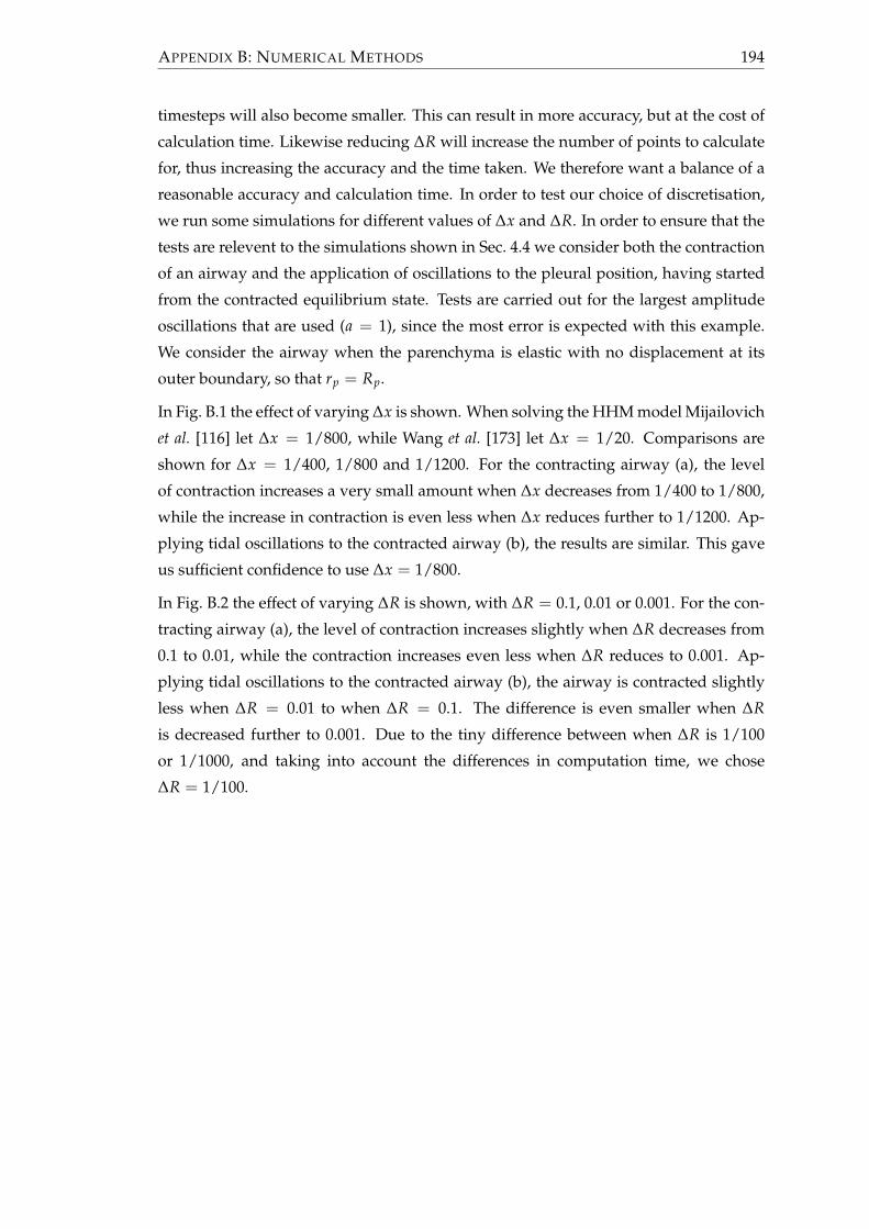
APPENDIX B: NUMERICAL METHODS 194
timesteps will also become smaller. This can result in more accuracy, but at the cost of
calculation time. Likewise reducing ∆R will increase the number of points to calculate
for, thus increasing the accuracy and the time taken. We therefore want a balance of a
reasonable accuracy and calculation time. In order to test our choice of discretisation,
we run some simulations for different values of ∆x and ∆R. In order to ensure that the
tests are relevent to the simulations shown in Sec. 4.4 we consider both the contraction
of an airway and the application of oscillations to the pleural position, having started
from the contracted equilibrium state. Tests are carried out for the largest amplitude
oscillations that are used (a = 1), since the most error is expected with this example.
We consider the airway when the parenchyma is elastic with no displacement at its
outer boundary, so that rp = Rp.
In Fig. B.1 the effect of varying ∆x is shown. When solving the HHM model Mijailovich
et al. [116] let ∆x = 1/800, while Wang et al. [173] let ∆x = 1/20. Comparisons are
shown for ∆x = 1/400, 1/800 and 1/1200. For the contracting airway (a), the level
of contraction increases a very small amount when ∆x decreases from 1/400 to 1/800,
while the increase in contraction is even less when ∆x reduces further to 1/1200. Ap-
plying tidal oscillations to the contracted airway (b), the results are similar. This gave
us sufficient confidence to use ∆x = 1/800.
In Fig. B.2 the effect of varying ∆R is shown, with ∆R = 0.1, 0.01 or 0.001. For the con-
tracting airway (a), the level of contraction increases slightly when ∆R decreases from
0.1 to 0.01, while the contraction increases even less when ∆R reduces to 0.001. Ap-
plying tidal oscillations to the contracted airway (b), the airway is contracted slightly
less when ∆R = 0.01 to when ∆R = 0.1. The difference is even smaller when ∆R
is decreased further to 0.001. Due to the tiny difference between when ∆R is 1/100
or 1/1000, and taking into account the differences in computation time, we chose
∆R = 1/100.
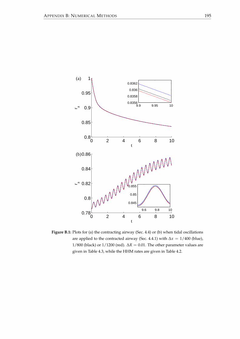
APPENDIX B: NUMERICAL METHODS 195
0 2 4 6 8 100.8
0.85
0.9
0.95
1
t
r a 9.9 9.95 100.8356
0.8358
0.836
0.8362(a)
0 2 4 6 8 100.78
0.8
0.82
0.84
0.86
t
r a
9.6 9.8 10
0.845
0.85
0.855
(b)
Figure B.1: Plots for (a) the contracting airway (Sec. 4.4) or (b) when tidal oscillations
are applied to the contracted airway (Sec. 4.4.1) with ∆x = 1/400 (blue),
1/800 (black) or 1/1200 (red). ∆R = 0.01. The other parameter values are
given in Table 4.3, while the HHM rates are given in Table 4.2.

APPENDIX B: NUMERICAL METHODS 196
0 2 4 6 8 100.8
0.85
0.9
0.95
1
t
r a 9.9 9.95 100.8356
0.8358
0.836
0.8362(a)
0 2 4 6 8 100.78
0.8
0.82
0.84
0.86
t
r a
9.6 9.8 10
0.845
0.85
0.855
(b)
Figure B.2: Plots for (a) the contracting airway (Sec. 4.4) or (b) when tidal oscillations
are applied to the contracted airway (Sec. 4.4.1) with ∆R = 0.1 (blue), 0.01
(black) or 0.01 (red). (The red and black lines overlap.) ∆x = 1/800. The
other parameter values are given in Table 4.3, while the HHM rates are
given in Table 4.2.

References
[1] A. Adler, E.A. Cowley, J.H.T. Bates, and D.H. Eidelman. Airway-parenchymal
interdependence after airway contraction in rat lung explants. Journal of Applied
Physiology, 85(1):231–237, 1998.
[2] D.A. Affonce and K.R. Lutchen. New perspectives on the mechanical basis for
airway hyperreactivity and airway hypersensitivity in asthma. Journal of Applied
Physiology, 101(6):1710–1719, 2006.
[3] D. Ambrosi and S. Pezzuto. Active stress vs. active strain in mechanobiology:
Constitutive issues. Journal of Elasticity, 107:199–212, 2012.
[4] J.R. Barber. Elasticity. Solid Mechanics and its Applications. Kluwer academic
publishers, second edition, 2002.
[5] P.J. Barnes, K.F. Chung, and C.P. Page. Inflammatory mediators of asthma: An
update. Pharmacological Reviews, 50(4):515–596, 1998.
[6] P.J. Barnes, B. Jonsson, and J.B. Klim. The costs of asthma. European Respiratory
Journal, 9(4):636–642, 1996.
[7] N.A. Barrett and K.F. Austen. Innate Cells and T Helper 2 Cell Immunity in
Airway Inflammation. Immunity, 31(3):425–437, 2009.
[8] J.H.T. Bates, S.R. Bullimore, A.Z. Politi, J. Sneyd, R.C. Anafi, and A.M. Lauzon.
Transient oscillatory force-length behavior of activated airway smooth muscle.
American Journal of Physiology. Lung Cellular and Molecular Physiology, 297(2):L362–
L372, 2009.
[9] E.H. Bel. Bronchial thermoplasty: Has the promise been met? American Journal
of Respiratory and Critical Care Medicine, 181(2):101–102, 2010.
[10] R. Berair, R. Saunders, and C.E. Brightling. Origins of increased airway smooth
muscle mass in asthma. BMC Medicine, 11:145, 2013.
197

REFERENCES 198
[11] C. Bergeron, W. Al-Ramli, and Q. Hamid. Remodeling in asthma. Proceedings of
the American Thoracic Society, 6(3):301–305, 2009.
[12] A. Bergner and M.J. Sanderson. Acetylcholine-induced calcium signaling and
contraction of airway smooth muscle cells in lung slices. The Journal of General
Physiology, 119:187–198, 2002.
[13] M.J. Berridge, P. Lipp, and M.D. Bootman. The versatility and universality of
calcium signalling. Nature Reviews Molecular Cell Biology, 1(1):11–21, 2000.
[14] J. Bousquet, P.K. Jeffery, W.W. Busse, M. Johnson, and A.M. Vignola. Asthma -
From bronchoconstriction to airways inflammation and remodeling. American
Journal of Respiratory and Critical Care Medicine, 161(5), 2000.
[15] J. Bousquet, E. Mantzouranis, A.A. Cruz, C.E. Aït-Khaled, N.and Baena-Cagnani,
E.R. Bleecker, C.E. Brightling, P. Burney, A. Bush, W.W. Busse, T.B. Casale,
M. Chan-Yeung, R. Chen, B. Chowdhury, K.F. Chung, R. Dahl, J.M. Drazen, L.M.
Fabbri, S.T. Holgate, F. Kauffmann, T. Haahtela, N. Khaltaev, J.P. Kiley, M.R. Mas-
jedi, Y. Mohammad, P. O’Byrne, M.R. Partridge, K.F. Rabe, A. Togias, C. van Weel,
S. Wenzel, N. Zhong, and T. Zuberbier. Uniform definition of asthma severity,
control, and exacerbations: Document presented for the world health organiza-
tion consultation on severe asthma. Journal of Allergy and Clinical Immunology,
126(5):926 – 938, 2010.
[16] R.N. Bracewell. The Fourier Transform and its Applications. McGraw-Hill Ko-
gakusha, Ltd., Tokyo, second edition, 1978.
[17] C.E. Brightling, S. Gupta, S. Gonem, and S. Siddiqui. Lung damage and air-
way remodelling in severe asthma. Clinical & Experimental Allergy, 42(5):638–649,
2012.
[18] British Thoracic Society. British guideline on the management of asthma: A na-
tional clinical guideline, 2009.
[19] British Thoracic Society COPD Consortium. Spirometry in practice: A practical
guide to using spirometry in primary care second edition, 2005.
[20] B.S. Brook, S.A.E.G. Falle, and T.J. Pedley. Numerical solutions for unsteady
gravity-driven flows in collapsible tubes: evolution and roll-wave instability of a
steady state. Journal of Fluid Mechanics, 396:223–256, 1999.
[21] B.S. Brook and O.E. Jensen. The role of contractile unit reorganization in force
generation in airway smooth muscle. Mathematical Medicine and Biology, 2013.

REFERENCES 199
[22] B.S. Brook, S.E. Peel, I.P. Hall, A.Z. Politi, J. Sneyd, Y. Bai, M.J. Sanderson, and
O.E. Jensen. A biomechanical model of agonist-initiated contraction in the asth-
matic airway. Respiratory Physiology & Neurobiology, 170(1):44 – 58, 2010.
[23] D. Bumbacea, D. Campbell, L. Nguyen, D. Carr, P.J. Barnes, D. Robinson, and
K.F. Chung. Parameters associated with persistent airflow obstruction in chronic
severe asthma. European Respiratory Journal, 24(1):122–128, 2004.
[24] J.P. Butler, I.M. Tolic-Nørrelykke, B. Fabry, and J.J. Fredberg. Traction fields, mo-
ments, and strain energy that cells exert on their surroundings. American Journal
of Physiology - Cell Physiology, 282(3):C595–C605, 2002.
[25] C. Calogero and P.D. Sly. Developmental physiology: Lung function during
growth and development from birth to old age. European Respiratory Society
Monograph, 47:1–15, 2010.
[26] P.G. Ciarlet and G. Geymonat. Sur les lois de comportement en élasticité non
linéaire compressible. Comptes-rendus de l’Académie des Sciences de Paris Série II,
295:423–426, 1982.
[27] S.L. Codd, R.K. Lambert, M.R. Alley, and R.J. Pack. Tensile stiffness of ovine
tracheal wall. Journal of Applied Physiology, 76(6):2627–2635, 1994.
[28] M.F. Coughlin, B. Suki, and D. Stamenovic. Dynamic behavior of lung
parenchyma in shear. Journal of Applied Physiology, 80(6):1880–1890, 1996.
[29] R. Courant, E. Isaacson, and M. Rees. On the solution of nonlinear hyperbolic
differential equations by finite differences. Communications on Pure and Applied
Mathematics, 5(3):243–255, 1952.
[30] G. Cox, J.D. Miller, A. McWilliams, J.M. FitzGerald, and S. Lam. Bronchial ther-
moplasty for asthma. American Journal of Respiratory and Critical Care Medicine,
173(9):965–969, 2006.
[31] R.G. Crystal, J.B. West, P.J. Barnes, and E.R. Weibel, editors. The Lung: Scientific
Foundations. Raven Press Ltd., New York, 1991.
[32] D.E. Davies, J. Wicks, R.M. Powell, S.M. Puddicombe, and S.T. Holgate. Airway
remodeling in asthma: New insights. Journal of Allergy and Clinical Immunology,
111(2):215–225, 2003.
[33] J.C. de Jongste, R. van Strik, I.L. Bonta, and K.F. Kerrebijn. Measurement of hu-
man small airway smooth muscle function in vitro with the bronchiolar strip
preparation. Journal of Pharmacological Methods, 14(2):111 – 118, 1985.

REFERENCES 200
[34] J.G.R. Demonchy, H.F. Kauffman, P. Venge, G.H. Koeter, H.M. Jansen, H.J. Sluiter,
and K. Devries. Bronchoalveolar eosinophilia during allergen-induced late asth-
matic reactions. American Review of Respiratory Disease, 131(3):373–376, 1985.
[35] A. Dietrich, V. Chubanov, H. Kalwa, B.R. Rost, and T. Gudermann. Cation chan-
nels of the transient receptor potential superfamily: Their role in physiological
and pathophysiological processes of smooth muscle cells. Pharmacology & Thera-
peutics, 112(3):744–760, 2006.
[36] E.H. Dill. Continuum mechanics: elasticity, plasticity, viscoelasticity. CRC Press, Boca
Raton, Fl, 2007.
[37] P.F. Dillon, M.O. Aksoy, S.P. Driska, and R.A. Murphy. Myosin phosphorylation
and the cross-bridge cycle in arterial smooth-muscle. Science, 211(4481):495–497,
1981.
[38] G.M. Donovan and M.H. Tawhai. A simplified model of airway narrowing due to
bronchial mucosal folding. Respiratory Physiology & Neurobiology, 171(2):144–150,
2010.
[39] M. Ebina, H. Yaegashi, T. Takahashi, M. Motomiya, and M. Tanemura. Distri-
bution of smooth muscles along the bronchial tree: A morphometric study of
ordinary autopsy lungs. American Journal of Respiratory and Critical Care Medicine,
141(5 Pt 1):1322–1326, 1990.
[40] B. Fabry and J.J. Fredberg. Remodeling of the airway smooth muscle cell: are we
built of glass? Respiratory Physiology & Neurobiology, 137(2-3):109–124, 2003.
[41] G. Farnebäck. Two-frame motion estimation based on polynomial expansion. In
J. Bigun and T. Gustavsson, editors, Image Analysis, volume 2749 of Lecture Notes
in Computer Science, pages 363–370. Springer Berlin Heidelberg, 2003.
[42] J. Fox. Utility of the precision cut lung slice model to investigate airway smooth muscle
contraction. PhD thesis, University of Nottingham, UK, 2011.
[43] J.J. Fredberg, D. Inouye, B. Miller, M. Nathan, S. Jafari, S.H. Raboudi, J.P. Butler,
and S.A. Shore. Airway smooth muscle, tidal stretches, and dynamically deter-
mined contractile states. American Journal of Respiratory and Critical Care Medicine,
156(6):1752–1759, 1997.
[44] J.J. Fredberg, D.S. Inouye, S.M. Mijailovich, and J.P. Butler. Perturbed equilib-
rium of myosin binding in airway smooth muscle and its implications in bron-

REFERENCES 201
chospasm. American Journal of Respiratory and Critical Care Medicine, 159(3):959–
967, 1999.
[45] Y.C. Fung. A theory of elasticity of the lung. Journal of Applied Mechanics, 41(1):8–
14, 1974.
[46] Y.C. Fung. Biomechanics, Mechanical Properties of Living Tissues. Springer-Verlag,
New York, second edition, 1993.
[47] T.C. Gasser, R.W. Ogden, and G.A. Holzapfel. Hyperelastic modelling of arterial
layers with distributed collagen fibre orientations. Journal of the Royal Society
Interface, 3(6):15–35, 2006.
[48] Global Initiative For Asthma. Pocket guide to asthma management and preven-
tion, 2010.
[49] J.B. Grotberg and S.H. Davis. Fluid-dynamical flapping of a collapsible channel:
sound generation and flow limitation. Journal of Biomechanics, 13:219–230, 1980.
[50] S. J. Gunst, J.Q. Stropp, and J. Service. Mechanical modulation of pressure-
volume characteristics of contracted canine airways in vitro. Journal of Applied
Physiology, 68:2223–2229, 1990.
[51] S.J. Gunst and D.D. Tang. The contractile apparatus and mechanical properties
of airway smooth muscle. European Respiratory Journal, 15(3):600–616, 2000.
[52] C.M. Hai and R.A. Murphy. Cross-bridge phosphorylation and regulation of
latch state in smooth-muscle. American Journal of Physiology, 254(1 Pt 1):C99–
C106, 1988.
[53] C.M. Hai and R.A. Murphy. Regulation of shortening velocity by cross-bridge
phosphorylation in smooth muscle. American Journal of Physiology - Cell Physiol-
ogy, 255(1):C86–C94, 1988.
[54] H. Hammad and B.N. Lambrecht. Dendritic cells and epithelial cells: linking
innate and adaptive immunity in asthma. Nature Reviews Immunology, 8(3):193–
204, 2008.
[55] A. Harten, P. Lax, and B. Leer. On upstream differencing and godunov-type
schemes for hyperbolic conservation laws. SIAM Review, 25(1):35–61, 1983.
[56] M. Heil, A.L. Hazel, and J.A. Smith. The mechanics of airway closure. Respiratory
Physiology & Neurobiology, 163(1-3):214 – 221, 2008.

REFERENCES 202
[57] A.M. Herrera, B.E. McParland, A. Bienkowska, R. Tait, P.D. Paré, and C.Y. Seow.
‘Sarcomeres’ of smooth muscle: functional characteristics and ultrastructural ev-
idence. Journal of Cell Science, 118(11):2381–2392, 2005.
[58] S.J. Hirst. Airway smooth muscle as a target in asthma. Clinical and Experimental
Allergy, 30:54–59, 2000.
[59] S.T Holgate. The airway epithelium is central to the pathogenesis of asthma. Al-
lergology International : official journal of the Japanese Society of Allergology, 57(1):1–
10, 2008.
[60] S.T. Holgate and R. Polosa. Treatment strategies for allergy and asthma. Nature
Reviews Immunology, 8(3):218–230, 2008.
[61] G. Holzapfel, T. Gasser, and R. Ogden. A new constitutive framework for arterial
wall mechanics and a comparative study of material models. Journal of Elasticity,
61(1):1–48, 2000.
[62] G.A. Holzapfel. Nonlinear solid mechanics : a continuum approach for engineering.
Wiley, Chichester, 2000.
[63] G.A. Holzapfel and R.W. Ogden. Constitutive modelling of arteries. Proceedings
of the Royal Society A-Mathematical physical and engineering sciences, 466:1551–1597,
2010.
[64] F.G. Hoppin. Parenchymal mechanics and asthma. Chest, 107(3 Suppl):S140–
S144, 1995.
[65] F.G. Hoppin, G.C. Lee, and S.V. Dawson. Properties of lung parenchyma in dis-
tortion. Journal of Applied Physiology, 39(5):742–751, 1975.
[66] P. Howell, G. Kozyreff, and J. Ockendon. Applied Solid Mechanics. Cambridge
University Press, Cambridge, 2009.
[67] J.D. Humphrey and S.L. Delange. An Introduction to Biomechanics: Solids and Flu-
ids, Analysis and Design. Springer, 2004.
[68] A.F. Huxley. Muscle structure and theories of contraction. Progress in Biophysics
& Molecular Biology, 7:255–&, 1957.
[69] R.E. Hyatt, T.A. Wilson, and E. Bar-Yishay. Prediction of maximal expiratory flow
in excised human lungs. Journal of Applied Physiology, 48(6):991–998, 1980.

REFERENCES 203
[70] H. Itoh, M. Nishino, and H. Hatabu. Architecture of the lung - Morphology and
function. Journal of Thoracic Imaging, 19(4):221–227, 2004.
[71] L.J. Janssen and K. Killian. Airway smooth muscle as a target of asthma therapy:
history and new directions. Respiratory Research, 7(123), 2006.
[72] P.K. Jeffery. Remodeling in asthma and chronic obstructive lung disease. Ameri-
can Journal of Respiratory and Critical Care Medicine, 164(10, S):S28–S38, 2001.
[73] B. Jonson and C. Svantesson. Elastic pressure-volume curves: what information
do they convey? Thorax, 54(1):82–87, 1999.
[74] J.A. Jude, M.E. Wylam, T.F. Walseth, and M.S. Kannan. Calcium signaling in
airway smooth muscle. Proceedings of the American Thoracic Society, 5(1):15–22,
2008.
[75] K.E. Kadler, D.F. Holmes, J.A. Trotter, and J.A. Chapman. Collagen fibril forma-
tion. Biomedical Journal, 316(Pt 1):1–11, 1996.
[76] M. Kaliske and H. Rothert. Formulation and implementation of three-
dimensional viscoelasticity at small and finite strains. Computational Mechanics,
19(3):228–239, 1997.
[77] K.E. Kamm and J.T. Stull. Activation of smooth-muscle contraction - relation
between myosin phosphorylation and stiffness. Science, 232:80–82, 1986.
[78] R.D. Kamm. Airway wall mechanics. Annual Review of Biomedical Engineering,
1:47–72, 1999.
[79] R.D. Kamm and T.J. Pedley. Flow in collapsible tubes: a brief review. Journal of
Biomechanical Engineering, 111:177–179, 1989.
[80] J. Keener and J. Sneyd. Mathematical Physiology II: Systems Physiology 2nd ed.
Springer, New York, 2009.
[81] H.Y. Kim, R.H. DeKruyff, and D.T. Umetsu. The many paths to asthma: pheno-
type shaped by innate and adaptive immunity. Nature Immunology, 11(7):577–584,
2010.
[82] G.G. King, P.D. Paré, and C.Y. Seow. The mechanics of exageratted airway nar-
rowing in asthma: the role of smooth muscle. Respiration Physiology, 118:1–13,
1999.
REFERENCES 204
[83] M. Kroon. A constitutive model for smooth muscle including active tone and
passive viscoelastic behaviour. Mathematical Medicine and Biology-A Journal of the
IMA, 27(2):129–155, 2010.
[84] M. Kroon. Influence of dispersion in myosin filament orientation and anisotropic
filament contractions in smooth muscle. Journal of Theoretical Biology, 272(1):72 –
82, 2011.
[85] M. Kroon. Optimal length of smooth muscle assessed by a microstructurally and
statistically based constitutive model. Computer Methods in Biomedical Engineer-
ing, 14(1):43–52, 2011.
[86] K.-H. Kuo, A.M. Herrera, and C.Y. Seow. Ultrastructure of airway smooth mus-
cle. Respiratory Physiology & Neurobiology, 137(2-3):197–208, 2003.
[87] K.-H. Kuo and C.Y. Seow. Contractile filament architecture and force transmis-
sion in swine airway smooth muscle. Journal of Cell Science, 117(8):1503–1511,
2004.
[88] K.-H. Kuo, L. Wang, P.D. Paré, L.E. Ford, and C.Y. Seow. Myosin thick filament
lability induced by mechanical strain in airway smooth muscle. Journal of Applied
Physiology, 90(5):1811–1816, 2001.
[89] K. Kuwano, C.H. Bosken, P.D. Paré, T.R. Bai, B.R. Wiggs, and J.C. Hogg. Small
airways dimensions in asthma and in chronic obstructive pulmonary disease.
American Journal of Respiratory and Critical Care Medicine, 148(5):1220–1225, 1993.
[90] S.J. Lai-Fook. Lung parenchyma described as a prestressed compressible mate-
rial. Journal of Biomechanics, 10:357–365, 1977.
[91] S.J. Lai-Fook, R.E. Hyatt, J.R. Rodarte, and T.A. Wilson. Behavior of artificially
produced holes in lung parenchyma. Journal of Applied Physiology, 43(4):648–655,
1977.
[92] S.J. Lai-Fook, T.A. Wilson, R.E. Hyatt, and J.R. Rodarte. Elastic constants of in-
flated lobes of dog lungs. Journal of Applied Physiology, 40(4):508–513, 1976.
[93] R. Lakes. Viscoelastic Materials. Cambridge University Press, Cambridge, 2009.
[94] R.K. Lambert. Sensitivity and specificity of the computational model for maximal
expiratory flow. Journal of Applied Physiology, 57(4):958–970, 1984.
[95] R.K. Lambert, R.G. Castile, and R.S. Tepper. Model of forced expiratory flows and
airway geometry in infants. Journal of Applied Physiology, 96(2):688–692, 2004.

REFERENCES 205
[96] R.K. Lambert and T.A. Wilson. A model for the elastic properties of the lung and
their effect on expiratory flow. Journal of Applied Physiology, 34:34–48, 1973.
[97] R.K. Lambert and T.A. Wilson. Smooth muscle dynamics and maximal expira-
tory flow in asthma. Journal of Applied Physiology, 99(5):1885–1890, 2005.
[98] R.K. Lambert, T.A. Wilson, R.E. Hyatt, and J.R. Rodarte. A computational model
for expiratory flow. Journal of Applied Physiology, 52(1):44–56, 1982.
[99] B. Lande and W. Mitzner. Analysis of lung parenchyma as a parametric porous
medium. Journal of Applied Physiology, 101:926–933, 2006.
[100] A.S. LaPrad and K.R. Lutchen. The dissolution of intact airway responsiveness
from breathing fluctuations: what went wrong? Journal of Applied Physiology,
110(6):1506–1507, 2011.
[101] A.S. LaPrad, K.R. Lutchen, and B. Suki. A mechanical design principle for tissue
structure and function in the airway tree. PLoS Computational Biology, 9(5), 2013.
[102] A.S. LaPrad, T.L. Szabo, B. Suki, and K.R. Lutchen. Reply to noble, hernandez,
mitchell, and janssen. Journal of Applied Physiology, 109(3):940–941, 2010.
[103] A.S. LaPrad, T.L. Szabo, B. Suki, and K.R. Lutchen. Tidal stretches do not mod-
ulate responsiveness of intact airways in vitro. Journal of Applied Physiology,
109(2):295–304, 2010.
[104] J. Latourelle, Fabry B., and J.J. Fredberg. Dynamic equilibration of airway smooth
muscle contraction during physiological loading. Journal of Applied Physiology,
92(2):771–779, 2002.
[105] T.L. Lavoie, R. Krishnan, H.R. Siegel, E.D. Maston, J.J. Fredberg, J. Solway, and
M.L. Dowell. Dilatation of the constricted human airway by tidal expansion
of lung parenchyma. American Journal of Respiratory and Critical Care Medicine,
186(3):225–232, 2012.
[106] M. Lei, H. Ghezzo, M.F. Chen, and D.H. Eidelman. Airway smooth muscle ori-
entation in intraparenchymal airways. Journal of Applied Physiology, 82(1):70–77,
1997.
[107] T.K. Lim, N.B. Pride, and J.R.J. Inram. Effects of volume history during sponta-
neous and acutely induced air-flow obstruction in asthma. The American Review
of Respiratory Disease, 135:591–596, 1987.

REFERENCES 206
[108] B. Ma and J.H.T. Bates. Continuum vs. spring network models of airway-
parenchymal interdependence. Journal of Applied Physiology, 113(1):124–129, 2012.
[109] B. Ma, M. Sanderson, and J.H.T. Bates. Airway-parenchymal interdependence in
the lung slice. Respiratory Physiology & Neurobiology, 185(2):211 – 216, 2013.
[110] L. Marcucci and L. Truskinovsky. Mechanics of the power stroke in myosin II.
Physical Review E, 81(051915), 2010.
[111] L. Marcucci and L. Truskinovsky. Muscle contraction: A mechanical perspective.
The European Physical Journal E, 32:411–418, 2010.
[112] R. Marshall and J.G. Widdicombe. Stress relaxation of human lung. Clinical Sci-
ence, 20(1):19–31, 1961.
[113] J. Mead, T. Takishima, and D. Leith. Stress distribution in lungs: a model of
pulmonary elasticity. Journal of Applied Physiology, 28(5):596–608, 1970.
[114] D. Mehta and S.J. Gunst. Actin polymerization stimulated by contractile activa-
tion regulates force development in canine tracheal smooth muscle. The Journal
of Physiology, 519(3):829–840, 1999.
[115] R.R. Mercer and J.D. Crapo. Spatial distribution of collagen and elastin fibers in
the lungs. Journal of Applied Physiology, 69(2):756–765, 1990.
[116] S.M. Mijailovich, J.P. Butler, and J.J. Fredberg. Perturbed equilibria of myosin
binding in airway smooth muscle: Bond-length distributions, mechanics, and
atp metabolism. Biophysical Journal, 79(5):2667 – 2681, 2000.
[117] K.L. Moore and T.V.N. Persaud. The developing human : clinically oriented embryol-
ogy. Elsevier Mosby, Philadelphia, eighth edition, 2008.
[118] H. Motulsky and A. Christopoulos. Fitting models to biological data using linear
and nonlinear regression: a practical guide to curve fitting. Oxford University Press,
Oxford, 2004.
[119] D.E. Moulton and A. Goriely. Possible role of differential growth in airway wall
remodeling in asthma. Journal of Applied Physiology, 110(4):1003–1012, 2011.
[120] S.-I. Murtada, M. Kroon, and G.A. Holzapfel. A calcium-driven mechanochemi-
cal model for prediction of force generation in smooth muscle. Biomechanics and
Modeling in Mechanobiology, 9(6):749–762, 2010.

REFERENCES 207
[121] S.-I. Murtada, M. Kroon, and G.A. Holzapfel. Modeling the dispersion effects of
contractile fibers in smooth muscles. Journal of the Mechanics and Physics of Solids,
58(12):2065 – 2082, 2010.
[122] J.A. Nadel and D.F. Tierney. Effect of a previous deep inspiration on airway
resistance in man. Journal of Applied Physiology, 16:717–719, 1966.
[123] P. Nardinocchi and L. Teresi. On the active response of soft living tissues. Journal
of Elasticity, 88(1):27–39, 2007.
[124] P.B. Noble, J.M. Hernandez, H.W. Mitchell, and L.J. Janssen. Deep inspiration
and airway physiology: human, canine, porcine, or bovine? Journal of Applied
Physiology, 109(3):938–939, 2010.
[125] P.B. Noble, R.L. Jones, E.T. Needi, A. Cairncross, H.W. Mitchell, A.L. James, and
P.K. McFawn. Responsiveness of the human airway in vitro during deep inspi-
ration and tidal oscillation. Journal of Applied Physiology, 110(6):1510–1518, 2011.
[126] P.M. O’Byrne and M.D. Inman. Airway hyperresponsiveness. Chest, 123(3
Suppl):S411–S416.
[127] R.W. Ogden. Large deformation isotropic elasticity - on the correlation of the-
ory and experiment for incompressible rubberlike solids. Proceedings of the Royal
Society of London. A. Mathematical and Physical Sciences, 326(1567):565–584, 1972.
[128] R.W. Ogden. Nonlinear elasticity, anisotropy, material stability and residual
stresses in soft tissue. In G. Holzapfel and R.W. Ogden, editors, Biomechanics of
Soft Tissue in Cardiovascular Systems, number 441 in CISM Courses and Lectures,
pages 65–108. Springer-Verlag, 2003.
[129] M.N. Oliver, B. Fabry, A. Marinkovic, S.M. Mijailovich, J.P. Butler, and J.J. Fred-
berg. Airway hyperresponsiveness, remodeling, and smooth muscle mass right
answer, wrong reason? American Journal of Respiratory Cell and Molecular Biology,
37(3):264–272, 2007.
[130] M.R. Owen and M.A. Lewis. The mechanics of lung tissue under high-frequency
ventilation. SIAM Journal on Applied Mathematics, 61:2001, 2001.
[131] M. Palmqvist, G. Persson, L. Lazer, J. Rosenborg, P. Larsson, and J. Lotvall. In-
haled dry-powder formoterol and salmeterol in asthmatic patients: onset of ac-
tion, duration of effect and potency. European Respiratory Journal, 10(11):2484–
2489, 1997.

REFERENCES 208
[132] A. Papi, S. Amadesi, P. Chitano, P. Boschetto, A. Ciaccia, P. Geppetti, L.M. Fabbri,
and C.E. Mapp. Bronchopulmonary inflammation and airway smooth muscle
hyperresponsiveness induced by nitrogen dioxide in guinea pigs. European Jour-
nal of Pharmacology, 374(2):241 – 247, 1999.
[133] R.M. Pascual and S.P. Peters. Airway remodeling contributes to the progressive
loss of lung function in asthma: An overview. Journal of Allergy and Clinical Im-
munology, 116(3):477–486, 2005.
[134] T.J. Pedley and X.Y. Luo. Modelling flow and oscillations in collapsible tubes.
Theoretical and Computational Fluid Dynamics, 10:277–294, 1998.
[135] J.J. Perez Fontan, A.O. Ray, and T.R. Oxland. Stress relaxation of the respiratory
system in developing piglets. Journal of Applied Physiology, 73(4):1297–1309, 1992.
[136] P.D. Phelan, C.F. Robertson, and A. Olinsky. The Melbourne asthma study: 1964-
1999. Journal of Allergy and Clinical Immunology, 109(2):189–194, 2002.
[137] S. Phipps, F. Benyahia, T.T. Ou, J. Barkans, D.S. Robinson, and A.B. Kay. Acute
allergen-induced airway remodeling in atopic asthma. American Journal of Respi-
ratory Cell and Molecular Biology, 31(6):626–632, 2004.
[138] A.C. Pipkin. Lectures on Viscoelasticity Theory. Springer-Verlag, New York, second
edition, 1986.
[139] G. Pocock and C.D. Richards. Human Physiology-The Basis of Medicine third edition.
Oxford University Press, Oxford, 2006.
[140] A.Z. Politi, G.M. Donovan, M.H. Tawhai, M.J. Sanderson, A.-M. Lauzon, J.H.T.
Bates, and J. Sneyd. A multiscale, spatially distributed model of asthmatic airway
hyper-responsiveness. Journal of Theoretical Biology, 266(4):614 – 624, 2010.
[141] A. Rachev and K. Hayashi. Theoretical study of the effects of vascular smooth
muscle contraction on strain and stress distributions in arteries. Annals of Biomed-
ical Engineering, 27(4):459–468, 1999.
[142] F. Rasmussen, D.R. Taylor, E.M. Flannery, J.O. Cowan, J.M. Greene, G.P. Herbi-
son, and M.R. Sears. Risk factors for airway remodeling in asthma manifested
by a low postbronchohator FEV1/vital capacity ratio - A longitudinal population
study from childhood to adulthood. American Journal of Respiratory and Critical
Care Medicine, 165(11):1480–1488, 2002.

REFERENCES 209
[143] S.I. Rennard. Repair mechanisms in asthma. Journal of Allergy and Clinical Im-
munology, 98(6 Pt 2), 1996.
[144] H.Y. Reynolds. Lung inflammation - normal host defense or a complication of
some diseases. Annual Review of Medicine, 38:295–323, 1987.
[145] W.R. Roche, R. Beasley, J.H. Williams, and S.T. Holgate. Subepithelial fibrosis in
the bronchi of asthmatics. Lancet, 1(8637):520–524, 1989.
[146] P.L. Roe. Characteristic-based schemes for the euler equations. Annual Review of
Fluid Mechanics, 18(1):337–365, 1986.
[147] D.F. Rogers. The airway goblet cell. International Journal of Biochemistry & Cell
Biology, 35(1):1–6, 2003.
[148] D.F. Rogers. Airway mucus hypersecretion in asthma: an undervalued pathol-
ogy? Current Opinion in Pharmacology, 4(3):241–250, 2004.
[149] J. Roig, R. Hernando, and R. Mora. Indacaterol, a novel once daily inhaled β2-
adrenoreceptor agonist. The Open Respiratory Medicine Journal, 3:27–30, 2009.
[150] A. Schmitz and M. Böl. On a phenomenological model for active smooth muscle
contraction. Journal of Biomechanics, 44(11):2090–2095, 2011.
[151] M.R. Sears. Lung function decline in asthma. European Respiratory Journal,
30(3):411–413, 2007.
[152] C.Y. Seow, V.R. Pratusevich, and L.E. Ford. Series-to-parallel transition in the
filament lattice of airway smooth muscle. Journal of Applied Physiology, 89(3):869–
876, 2000.
[153] M. Siklosi, O.E. Jensen, R.H. Tew, and A. Logg. Multiscale modeling of the acous-
tic properties of lung parenchyma. ESAIM: Proceedings, 23:78–97, 2008.
[154] S.M. Smiley-Jewell, M.U. Tran, A.J. Weir, Z.A. Johnson, L.S. Van Winkle, and C.G.
Plopper. Three-dimensional mapping of smooth muscle in the distal conducting
airways of mouse, rabbit, and monkey. Journal of Applied Physiology, 93(4):1506–
1514, 2002.
[155] I.S. Sokolnikoff. Mathematical theory of elasticity. McGraw-Hill, New York, second
edition, 1956.
[156] M.P. Sparrow, M. Weichselbaum, and P.B. McCray. Development of the innerva-
tion and airway smooth muscle in human fetal lung. American journal of respira-
tory cell and molecular biology, 20(4):550–560, 1999.

REFERENCES 210
[157] A.J.M. Spencer. Constitutive theory for strongly anisotropic solids. In A.J.M.
Spencer, editor, Continuum Theory of the Mechanics of Fibre-Reinforced Composites,
CISM Courses and Lectures No. 282, International Centre for Mechanical Sci-
ences, pages 1–32. Springer-Verlag, Wien, 1984.
[158] J. Stålhand, A. Klarbring, and G.A. Holzapfel. Smooth muscle contraction:
Mechanochemical formulation for homogeneous finite strains. Progress in Bio-
physics & Molecular Biology, 96(1-3):465–481, 2008.
[159] D. Stamenovic and T.A. Wilson. A strain energy function for lung parenchyma.
Journal of Biomechanical Engineering, 107(1):81–86, 1985.
[160] D. Stamenovic and D. Yager. Elastic properties of air- and liquid-filled lung
parenchyma. Journal of Applied Physiology, 65:2565–2570, 1988.
[161] S. Stanojevic, A. Wade, J. Stocks, J. Hankinson, A.L. Coates, H. Pan, M. Rosenthal,
M. Corey, P. Lebecque, and T.J. Cole. Reference ranges for spirometry across all
ages - A new approach. American Journal of Respiratory and Critical Care Medicine,
177(3):253–260, 2008.
[162] B.C. Starcher. Elastin and the lung. Thorax, 41(8):577–585, 1986.
[163] A. Stevens and J. Lowe. Human Histology. Elsevier Mosby, Philadelphia, third
edition, 2005.
[164] M.E. Strek. Difficult asthma. Proceedings of the American Thoracic Society, 3(1):116–
123, 2006.
[165] Y. Sumi and Q. Hamid. Airway remodeling in asthma. Allergology international :
official journal of the Japanese Society of Allergology, 56(4):341–348, 2007.
[166] L.A. Taber and R. Perucchio. Modeling heart development. Journal of Elasticity,
61(1-3):165–197, 2000.
[167] T. Takishima and J. Mead. Tests of a model of pulmonary elasticity. Journal of
Applied Physiology, 33:576–581, 1972.
[168] H. Tavana, D. Huh, J.B. Groberg, and S. Takayama. Microfluidics, lung surfactant,
and respiratory disorders. Labmedicine, 40(4):203–209, 2009.
[169] K.J. Taylor and A.R. Luksza. Peripheral-blood eosinophil counts and bronchial
responsiveness. Thorax, 42(6):452–456, 1987.

REFERENCES 211
[170] The National Centre for the Replacement, Refinement and and Re-
duction of Animals in Research. The challenge of animal research.
http://www.nc3rs.org.uk/landing.asp?id=2, 2009.
[171] P. Tonino, M. Simon, and R. Craig. Mass determination of native smooth mus-
cle myosin filaments by scanning transmission electron microscopy. Journal of
Molecular Biology, 318(4):999 – 1007, 2002.
[172] P. Tracqui and J. Ohayon. An integrated formulation of anisotropic force-calcium
relations driving spatio-temporal contractions of cardiac myocytes. Philosophical
Transactions of the Royal Society A-Mathematical Physical and Engineering Sciences,
367(1908):4887–4905, 2009.
[173] I. Wang, A.Z. Politi, N. Tania, Y. Bai, M.J. Sanderson, and J. Sneyd. A mathemati-
cal model of airway and pulmonary arteriole smooth muscle. Biophysical Journal,
94(6):2053–2064, 2008.
[174] L. Wang, P.D. Paré, and C.Y. Seow. Effects of length oscillation on the subsequent
force development in swine tracheal smooth muscle. Journal of Applied Physiology,
88(6):2246–2250, 2000.
[175] H.M. Warrick and J.A. Spudich. Myosin structure and function in cell motility.
Annual Review of Cell Biology, 3:379–422, 1987.
[176] E.R. Weibel. Morphometry of the human lung. Springer Verlag and Academic Press,
New York, 1963.
[177] S.E. Wenzel. Asthma: defining of the persistent adult phenotypes. Lancet,
368(9537):804–813, 2006.
[178] A.R. West, H.T. Syyong, S. Siddiqui, C.D. Pascoe, T.M. Murphy, H. Maarsingh,
L. Deng, G.N. Maksym, and Y. Bossé. Airway contractility and remodeling: Links
to asthma symptoms. Pulmonary Pharmacology & Therapeutics, 26(1):3 – 12, 2013.
[179] B.R. Wiggs, C.A. Hrousis, J.M. Drazen, and R.D. Kamm. On the mechanism of
mucosal folding in normal and asthmatic airways. Journal of Applied Physiology,
83(6):1814–1821, 1997.
[180] M.W. Wong. Discrete fourier analysis. Pseudo-differential operators: theory and
applications Vol.5. Birkhäuser, Basel, 2011.
[181] World Health Organisation. Asthma: fact sheet 307.
http://www.who.int/mediacentre/factsheets/fs307/en/index.html, May
2011.

REFERENCES 212
[182] Z.-X. Wu, J.S. Barker, T.P. Batchelor, and R.D. Dey. Interleukin (IL)-1 regulates
ozone-enhanced tracheal smooth muscle responsiveness by increasing substance
P (SP) production in intrinsic airway neurons of ferret. Respiratory Physiology &
Neurobiology , 164(3):300 – 311, 2008.
[183] J. Yang, J.W. Clark Jr., R.M. Bryan, and C. Robertson. The myogenic response
in isolated rat cerebrovascular arteries: smooth muscle cell model. Medical Engi-
neering & Physics, 25(8):691 – 709, 2003.
[184] J. Yang, J.W. Clark Jr., R.M. Bryan, and C.S. Robertson. The myogenic response in
isolated rat cerebrovascular arteries: vessel model. Medical Engineering & Physics,
25(8):711 – 717, 2003.
[185] M.A. Zulliger, A. Rachev, and N. Stergiopulos. A constitutive formulation of
arterial mechanics including vascular smooth muscle tone. American Journal of
Physiology-Heart and Circulatory Physiology, 287(3):H1335–H1343, 2004.