Hip Psychometrics

Peter BaldwinJoseph BernsteinHoward Wainer

Models vary in strength

When you have a lot of data, your need for a model decreases and so you can manage with a weak one.When your data are very limited, you need a strong model to lean on in order to draw inferences

A very strong model

P(x=1| ) = exp()/[1+ exp()] 0-PL

This is a strong model that requires few data to estimate its single parameter (person ability), but in return makes rigid assumptions about

the data (all items must be of equal difficulty). Such a model is justified only when you don’t have enough data to reject its assumptions.

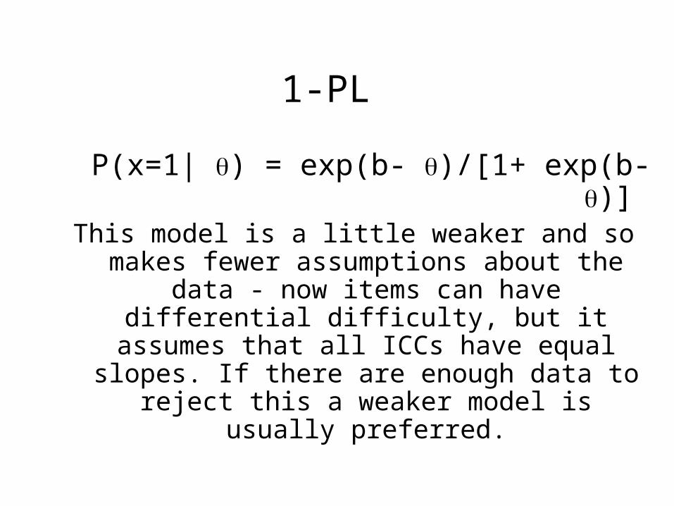
1-PL

P(x=1| ) = exp(b- )/[1+ exp(b- )]

This model is a little weaker and so makes fewer assumptions about the data - now

items can have differential difficulty, but it assumes that all ICCs have equal slopes. If

there are enough data to reject this a weaker model is usually preferred.

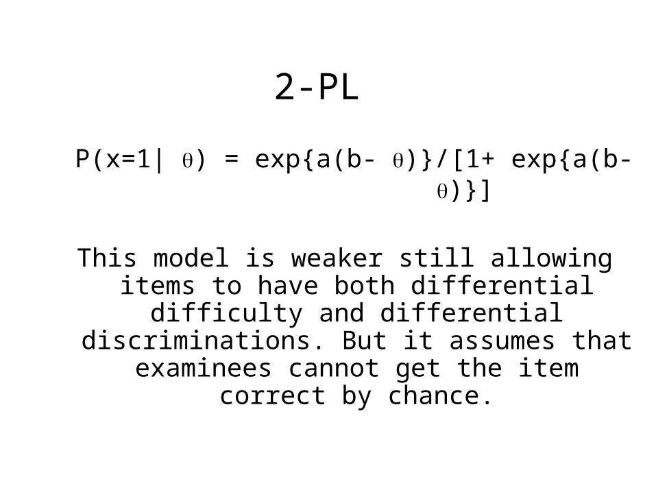
2-PL

P(x=1| ) = exp{a(b- )}/[1+ exp{a(b- )}]

This model is weaker still allowing items to have both differential difficulty and

differential discriminations. But it assumes that examinees cannot get the item

correct by chance.

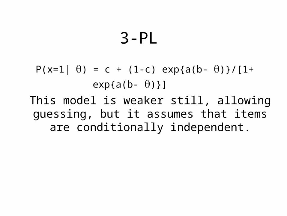
3-PL

P(x=1| ) = c + (1-c) exp{a(b- )}/[1+ exp{a(b- )}]

This model is weaker still, allowing guessing, but it assumes that items are

conditionally independent.

Turtles all the way down!

As the amount of data we have increases, we can test the assumptions of a model and are no longer

forced to use one that is unrealistic.In general we prefer the weakest model that our

data will allow.Thus we often fit a sequence of models and choose

the one whose fit no longer improves with more generality (further weakening).

We usually have three models

In order of increasing complexity they are:

1. The one we fit to the data,

2. The one we use to think about the data, and

3. The one that would actually generate the data.

When data are abundant relative to the number of questions asked of them, answers can be formulated using little more than those data.

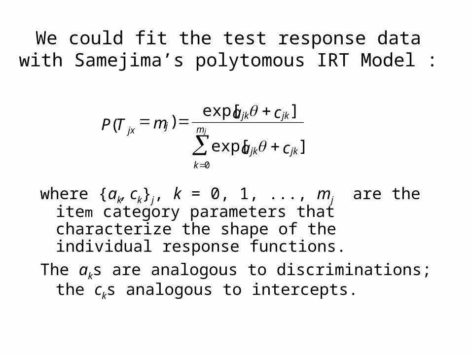
jxP(T jm ) exp[ jka jkc ]

exp[ jka jkc ]k0

jm

where {ak, ck}j, k = 0, 1, ..., mj are the item category parameters that characterize the shape of the individual response functions.

The aks are analogous to discriminations; the cks analogous to intercepts.

We could fit the test response data with Samejima’s polytomous IRT Model :

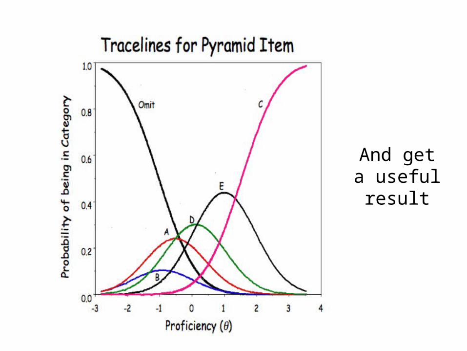
And get a useful result

But with 830,000 data points,

why bother?

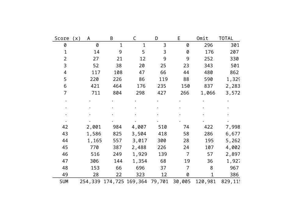
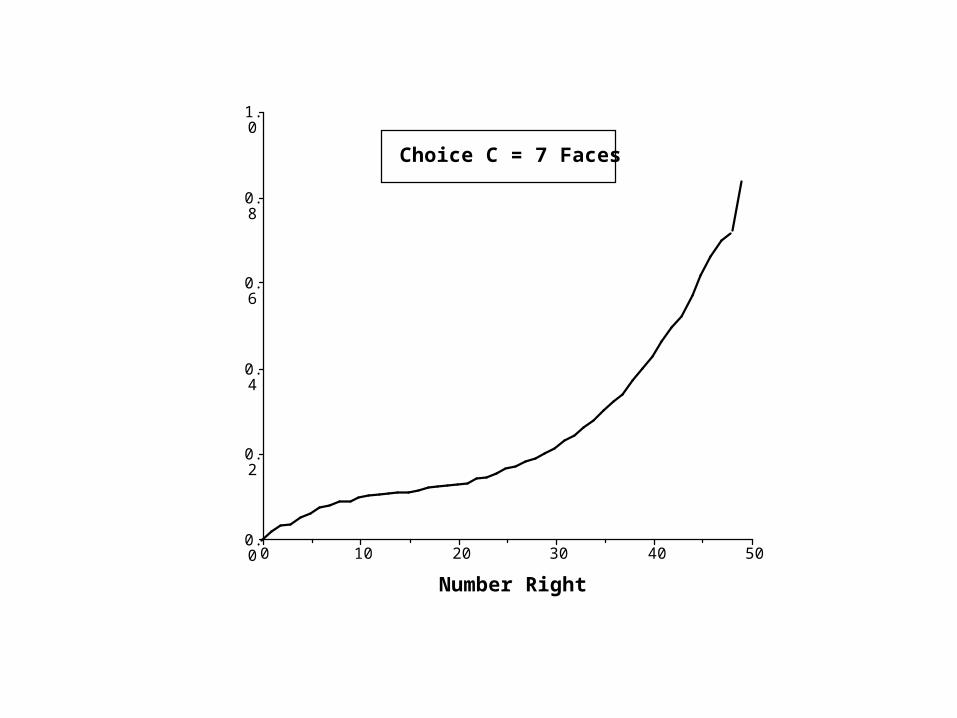
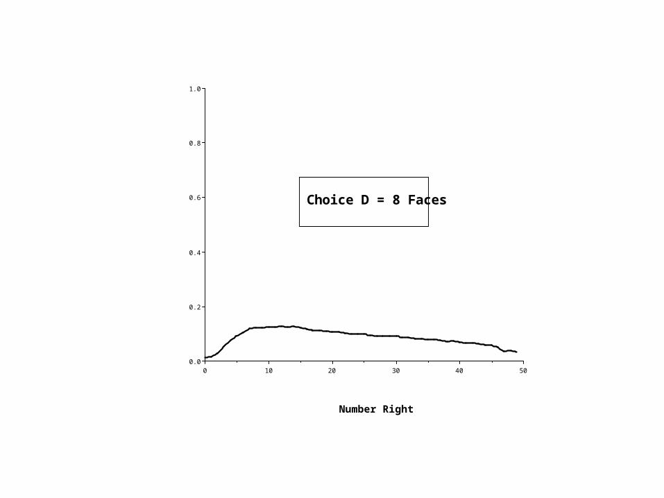
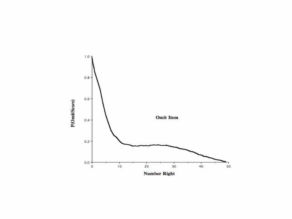
Score (x) A B C D E Omit TOTAL0 0 1 1 3 0 296 3011 14 9 5 3 0 176 2072 27 21 12 9 9 252 3303 52 38 20 25 23 343 5014 117 108 47 66 44 480 8625 220 226 86 119 88 590 1,3296 421 464 176 235 150 837 2,2837 711 804 298 427 266 1,066 3,572. . . . . . . .. . . . . . . .. . . . . . . .. . . . . . . .

42 2,001 984 4,007 510 74 422 7,99843 1,586 825 3,504 418 58 286 6,67744 1,165 557 3,017 300 28 195 5,26245 770 387 2,488 226 24 107 4,00246 516 249 1,929 139 7 57 2,89747 306 144 1,354 68 19 36 1,92748 153 66 696 37 7 8 96749 28 22 323 12 0 1 386

SUM 254,339 174,725 169,364 79,701 30,005 120,981 829,115

504030201000.0

0.2

0.4

0.6

0.8

1.0

Number Right

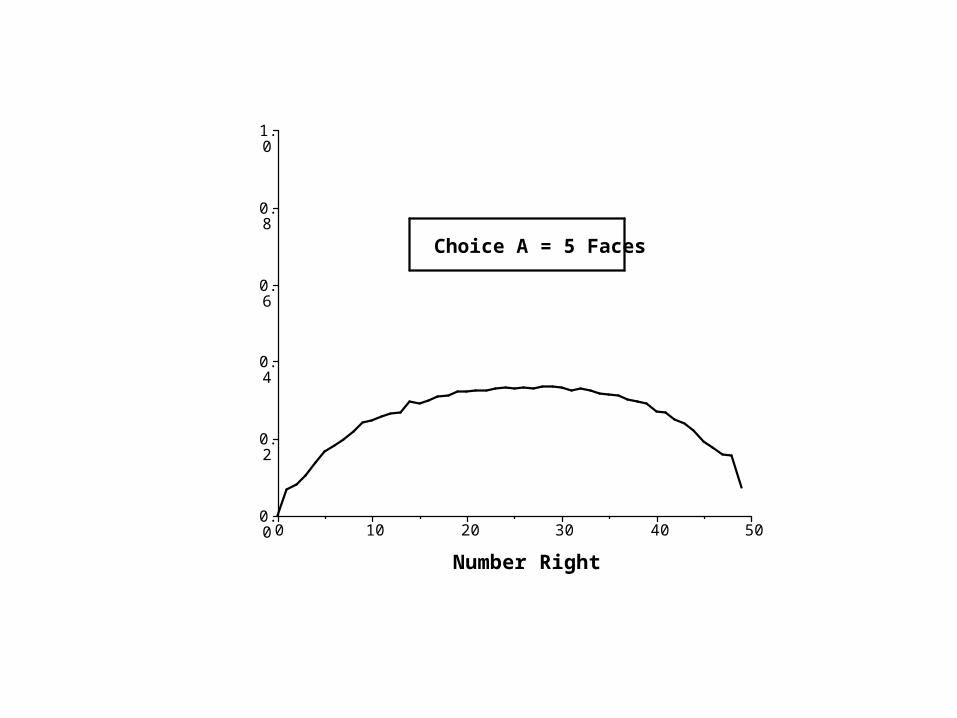
P(A

|sco

re)

Choice A = 5 Faces

504030201000.0

0.2

0.4

0.6

0.8

1.0

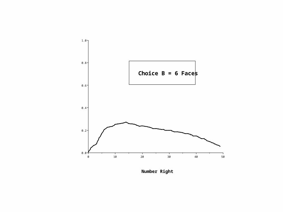
Choice B = 6 Faces

Number Right

P(B

|Sco

re)

504030201000.0

0.2

0.4

0.6

0.8

1.0

Number Right

P(C

|Sco

re)

Choice C = 7 Faces

504030201000.0

0.2

0.4

0.6

0.8

1.0

Choice D = 8 Faces

Number Right

P(D

|Sco

re)

504030201000.0

0.2

0.4

0.6

0.8

1.0

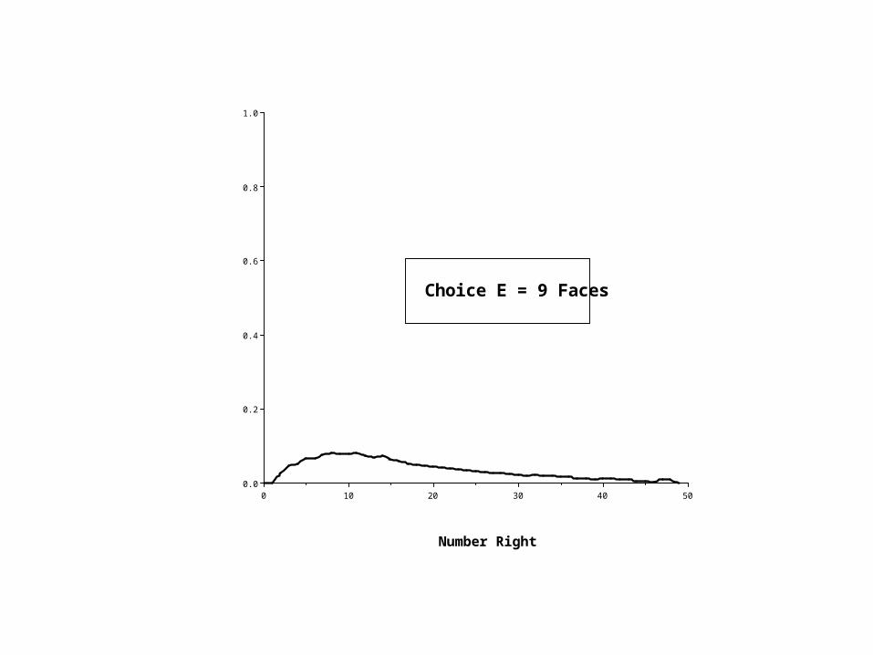
Choice E = 9 Faces

Number Right

P(E

|Sco

re)

A

D

E

B

C

E*

B*

C*

Proof that the correct answer is (A) Five

But when data are sparse, we must lean on strong models to

help us draw inferences.

A study of the diagnoses of hip fractures provides a compelling

illustration of the power of psychometric models to yield

insights when data are sparse.

Hip fractures are common injuries; more than 250,000 annually are treated in

the US alone. These fractures can be located in the shaft of the bone or in the neck of the bone connecting the shaft to the head

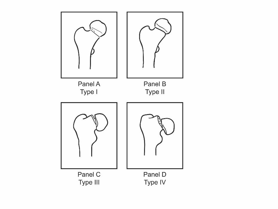
of the femur. Femoral neck fractures vary in their

severity

Garden (1961) provided a four-category classification scheme

for hip fractures.

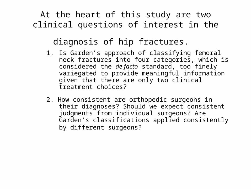
At the heart of this study are two clinical questions of interest in the diagnosis of hip

fractures. 1. Is Garden’s approach of classifying femoral neck

fractures into four categories, which is considered the de facto standard, too finely variegated to provide meaningful information given that there are only two clinical treatment choices?

2. How consistent are orthopedic surgeons in their diagnoses? Should we expect consistent judgments from individual surgeons? Are Garden’s classifications applied consistently by different surgeons?

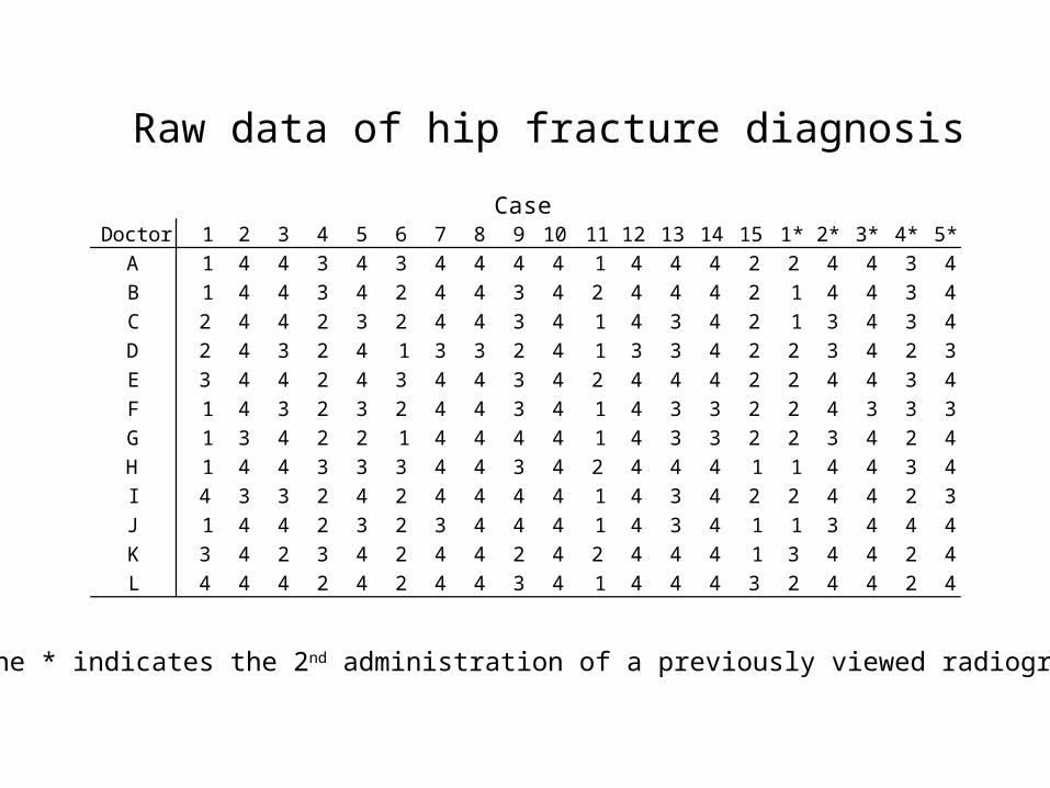
CaseDoctor 1 2 3 4 5 6 7 8 9 10 11 12 13 14 15 1* 2* 3* 4* 5*

A 1 4 4 3 4 3 4 4 4 4 1 4 4 4 2 2 4 4 3 4B 1 4 4 3 4 2 4 4 3 4 2 4 4 4 2 1 4 4 3 4C 2 4 4 2 3 2 4 4 3 4 1 4 3 4 2 1 3 4 3 4D 2 4 3 2 4 1 3 3 2 4 1 3 3 4 2 2 3 4 2 3E 3 4 4 2 4 3 4 4 3 4 2 4 4 4 2 2 4 4 3 4F 1 4 3 2 3 2 4 4 3 4 1 4 3 3 2 2 4 3 3 3G 1 3 4 2 2 1 4 4 4 4 1 4 3 3 2 2 3 4 2 4H 1 4 4 3 3 3 4 4 3 4 2 4 4 4 1 1 4 4 3 4I 4 3 3 2 4 2 4 4 4 4 1 4 3 4 2 2 4 4 2 3J 1 4 4 2 3 2 3 4 4 4 1 4 3 4 1 1 3 4 4 4K 3 4 2 3 4 2 4 4 2 4 2 4 4 4 1 3 4 4 2 4L 4 4 4 2 4 2 4 4 3 4 1 4 4 4 3 2 4 4 2 4

Raw data of hip fracture diagnosis

The * indicates the 2nd administration of a previously viewed radiograph

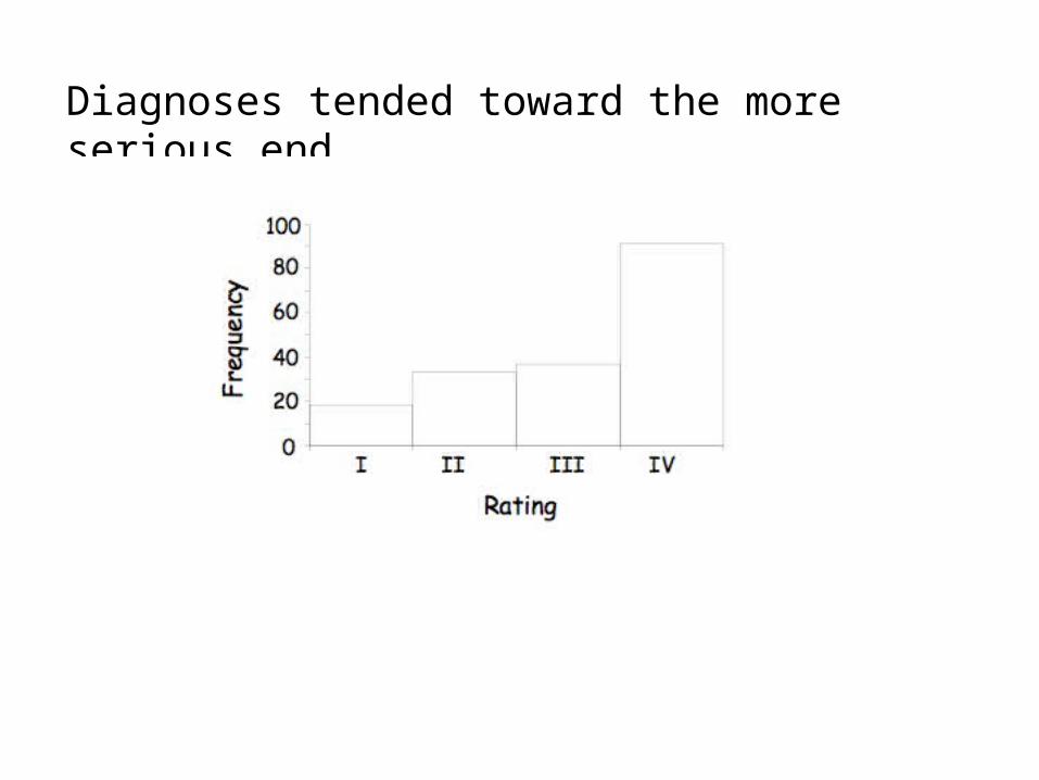
Diagnoses tended toward the more serious end

With 20 radiographs and only 12 judges how weak a model could we get away

with?

We wanted to use a Bayesian version of Samejima’s

polytomous model, but could we fit it with such sparse

data?

We decided to ask the experts.

We surveyed 42 of the world’s greatest experts in IRT, asking what would be the minimum ‘n’ required to obtain usefully

accurate results.

To summarize their advice

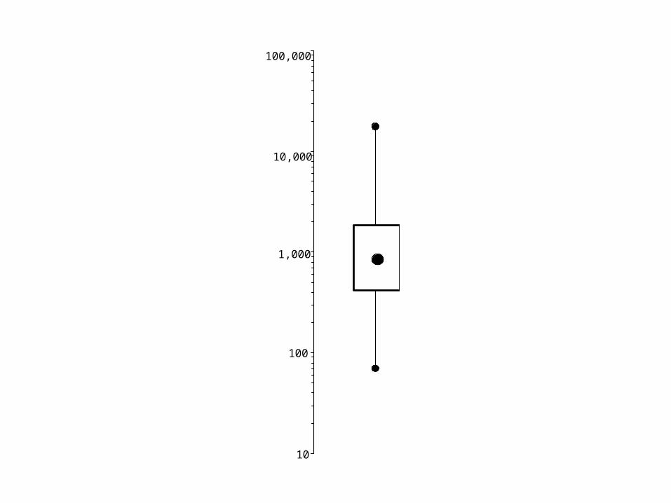
10

100

1,000

10,000

100,000

Min

imal A

ccep

tab

le S

am

ple

Siz

e

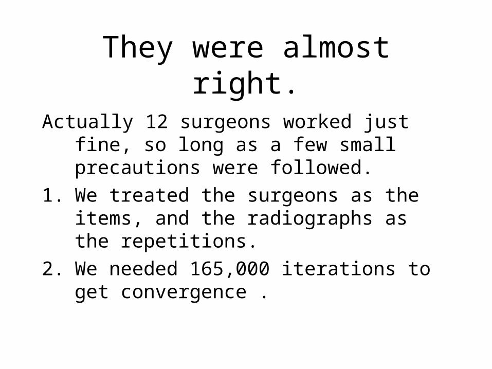
They were almost right.

Actually 12 surgeons worked just fine, so long as a few small precautions were followed.

1. We treated the surgeons as the items, and the radiographs as the repetitions.

2. We needed 165,000 iterations to get convergence .

Ethical Caveat

We feel obligated to offer the warnings that:

1. These analyses were performed by professionals; inexperienced persons should not attempt to duplicate them.

2. Keep MCMC software from out of the hands of amateurs and small children.

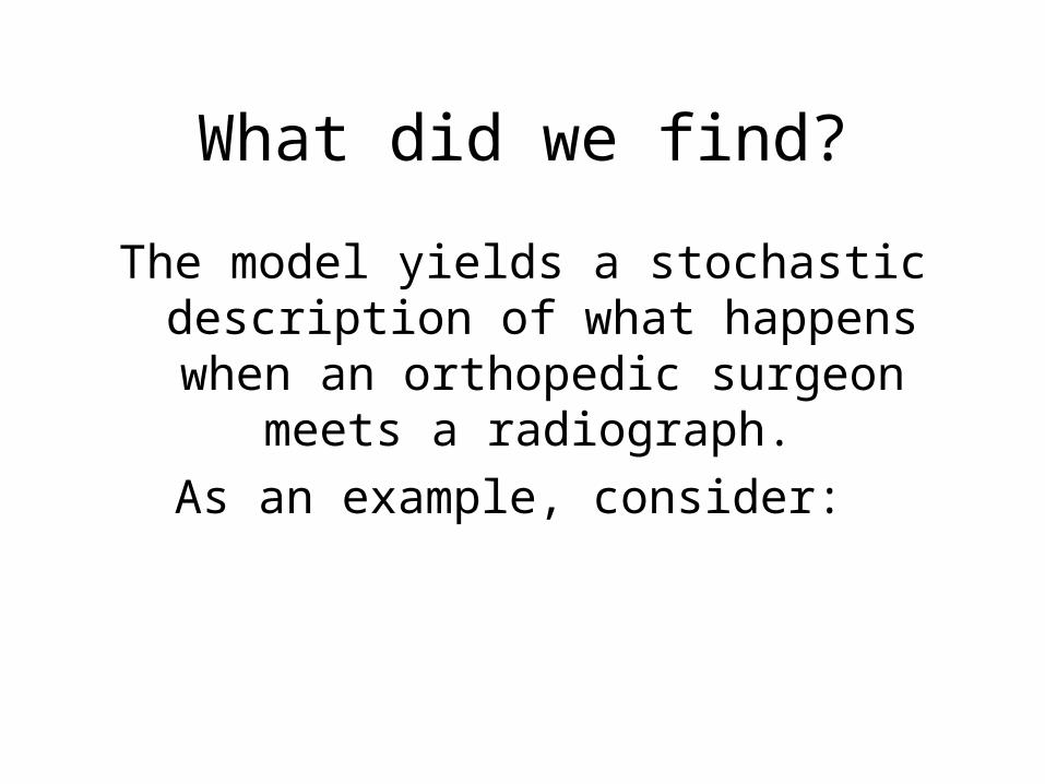
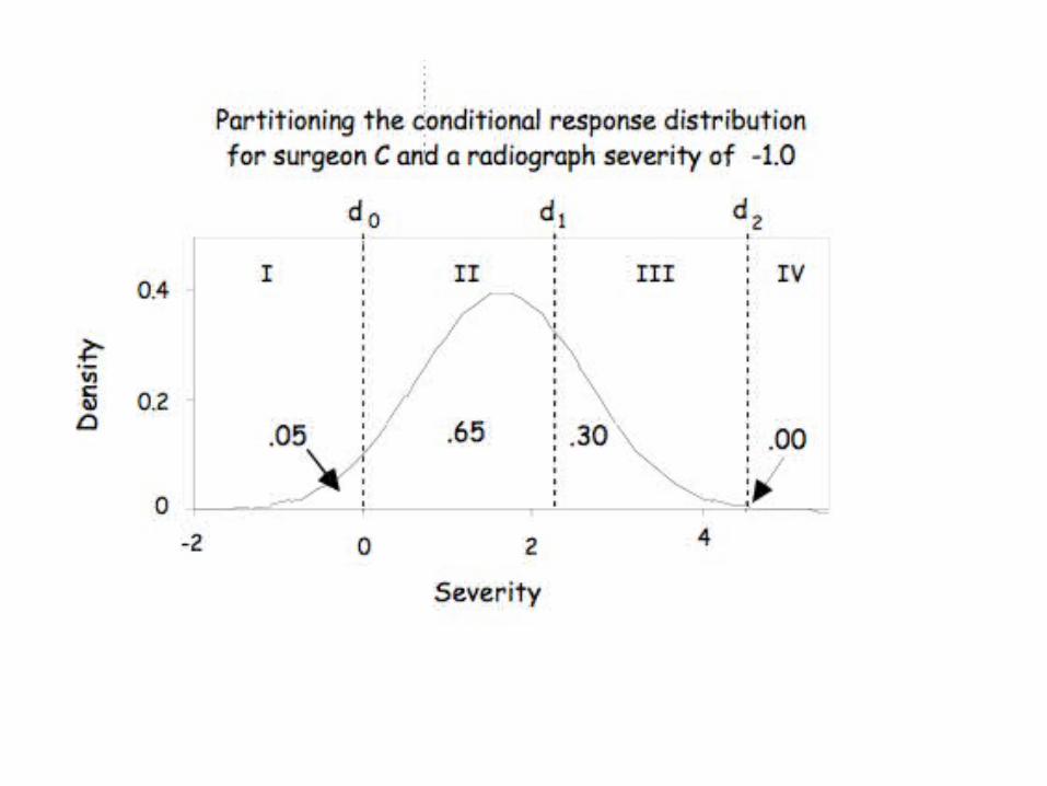
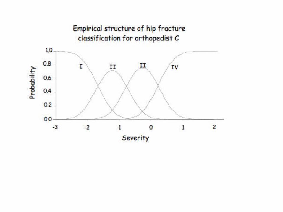
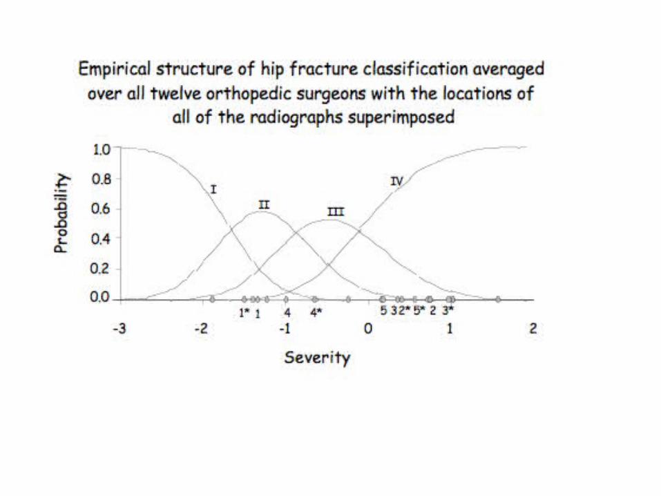
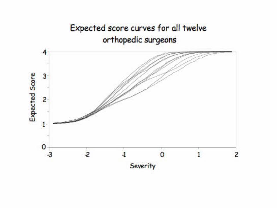
What did we find?

The model yields a stochastic description of what happens when

an orthopedic surgeon meets a radiograph.

As an example, consider:

Most of these results we could have gotten without the model. What

does fitting a psychometric model buy us?

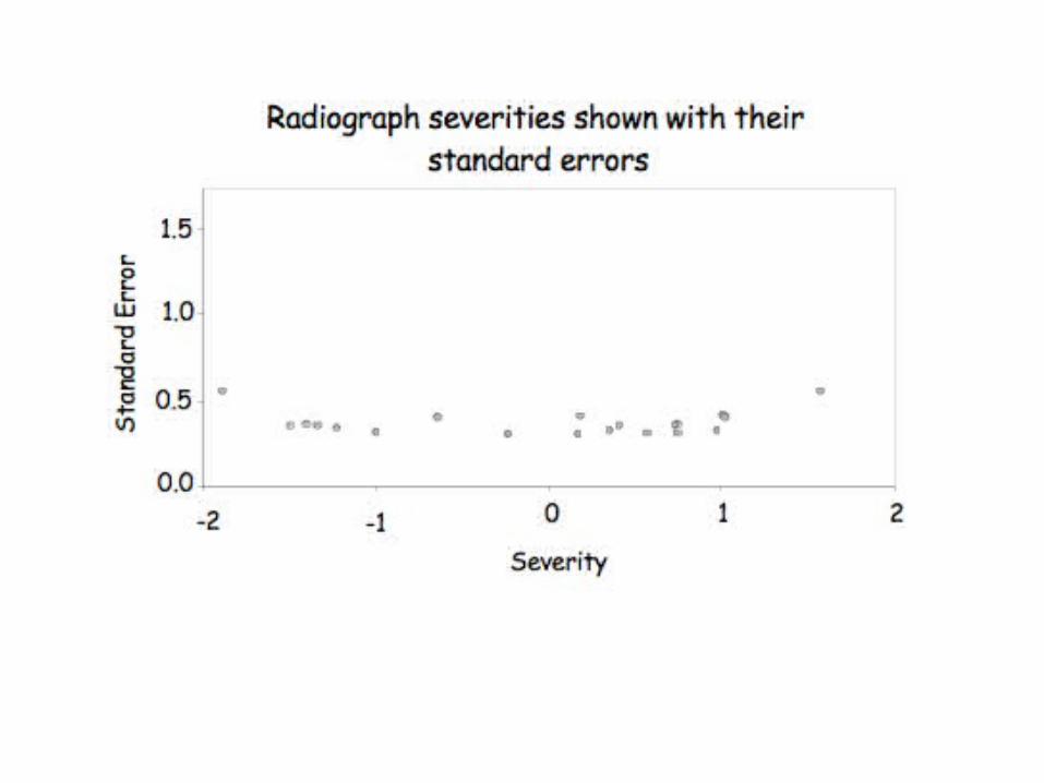
1. Standard errors - without a model all we can say is that different surgeons agree x% of the time on this radiograph. With a model we get more usable precision.

2. Automatic Adjustment for differential propensity for judging a fracture serious.

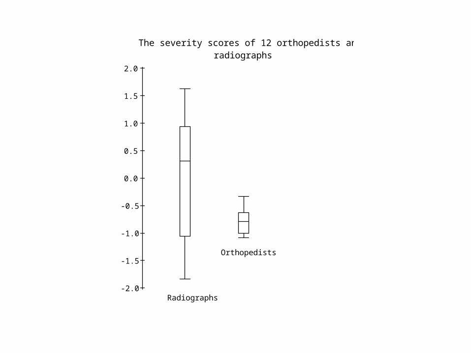
-2.0

-1.5

-1.0

-0.5

0.0

0.5

1.0

1.5

2.0

Radiographs

Orthopedists

The severity scores of 12 orthopedists and 15 radiographs

This is good news!

On essay scoring (and the scoring of most constructed response items)

the variance due to judges is usually about the same as the variance due to examinees.

Surgeons do much better than ‘expert judges.’

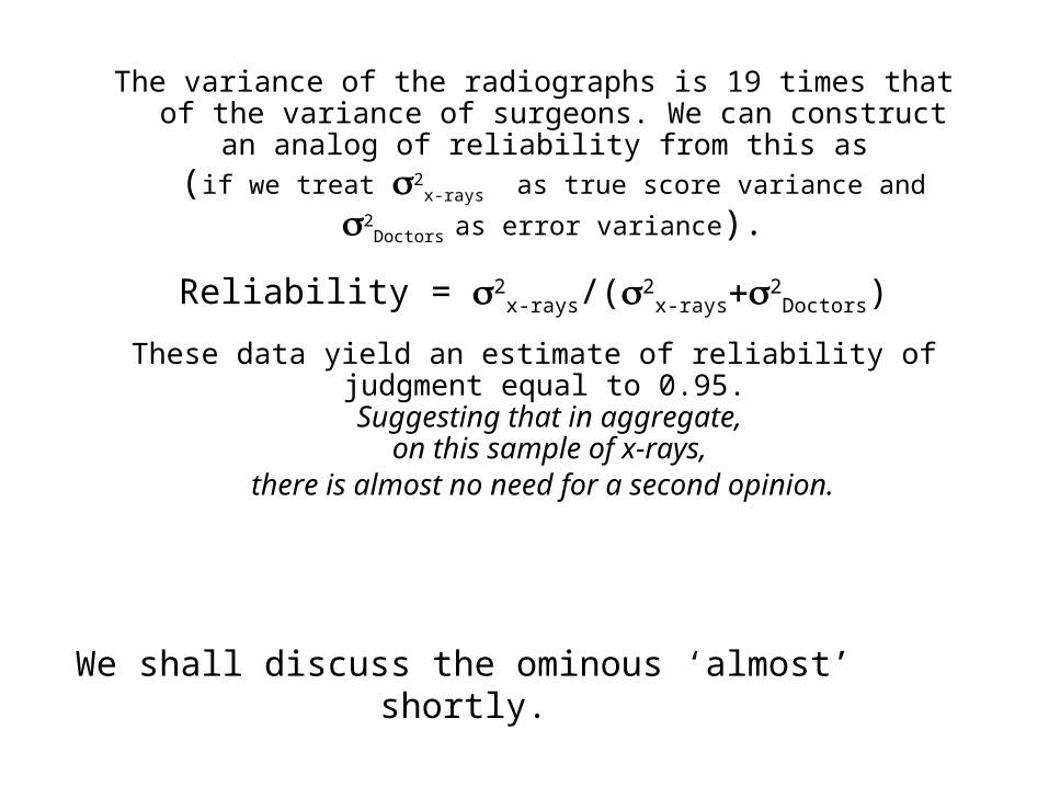
We shall discuss the ominous ‘almost’ shortly.

The variance of the radiographs is 19 times that of the variance of surgeons. We can construct an analog of

reliability from this as (if we treat 2

x-rays as true score variance and 2Doctors as error

variance).

Reliability = 2x-rays/(2

x-rays2Doctors)

These data yield an estimate of reliability of judgment equal to 0.95.

Suggesting that in aggregate, on this sample of x-rays,

there is almost no need for a second opinion.

The model provides us with robustness of judgment by adjusting the judgments for the

differences in the propensities of the orthopedists in their tendencies to vary in

severity.

For example, consider case 6. Although there are three doctors who judged it a III, the other nine all placed it as a I or a II.

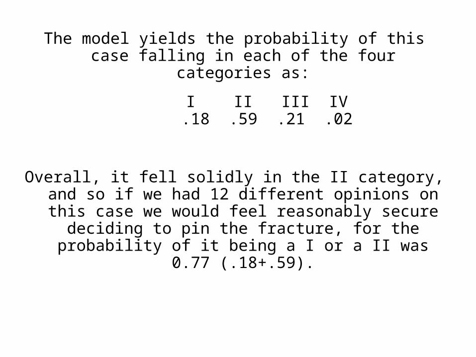
The model yields the probability of this case falling in each of the four categories as:

I II III IV.18 .59 .21 .02

Overall, it fell solidly in the II category, and so if we had 12 different opinions on this case we would

feel reasonably secure deciding to pin the fracture, for the probability of it being a I or a II

was 0.77 (.18+.59).

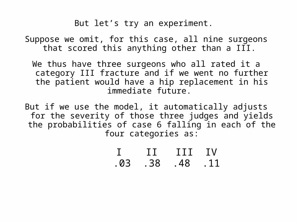
But let’s try an experiment.

Suppose we omit, for this case, all nine surgeons that scored this anything other than a III.

We thus have three surgeons who all rated it a category III fracture and if we went no further the patient would have a

hip replacement in his immediate future.

But if we use the model, it automatically adjusts for the severity of those three judges and yields the probabilities of

case 6 falling in each of the four categories as:

I II III IV.03 .38 .48 .11

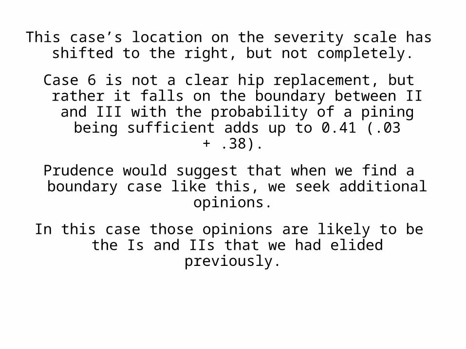
This case’s location on the severity scale has shifted to the right, but not completely.

Case 6 is not a clear hip replacement, but rather it falls on the boundary between II and III with the

probability of a pining being sufficient adds up to 0.41 (.03 + .38).

Prudence would suggest that when we find a boundary case like this, we seek additional

opinions.

In this case those opinions are likely to be the Is and IIs that we had elided previously.

Note that this yields deeper meaning to the phrase ‘second opinion’. It could mean getting more opinions from the same doctor on other cases so that we can

adjust his/her ratings for their any unusual severity.

This automatic adjustment is not easily available without an explicit model.

Last, the title of this talk could just as easily have been “Hearty Psychometrics” had the data we used been from 12 cardiac surgeons judging blood vessel blockage.

Peter and I are grateful to Joe for making us hip psychometricians and more grateful

still that Joe didn’t specialize in gastroenterology.