1

LBNL - 47066

Historical roots of gauge invariance

J. D. Jackson *University of California and Lawrence Berkeley National Laboratory, Berkeley, CA 94720

L. B. Okun Ê ITEP, 117218, Moscow, Russia

AAAABBBBSSSSTTTTRRRRAAAACCCCTTTTGauge invariance is the basis of the modern theory of electroweak and strong interactions (the socalled Standard Model). The roots of gauge invariance go back to the year 1820 whenelectromagnetism was discovered and the first electrodynamic theory was proposed. Subsequentdevelopments led to the discovery that different forms of the vector potential result in the sameobservable forces. The partial arbitrariness of the vector potential AAAA brought forth variousrestrictions on it. àààà °°°° AAAA = 0 was proposed by J. C. Maxwell; ǵA

µ = 0 was proposed L. V.

Lorenz in the middle of 1860's . In most of the modern texts the latter condition is attributed to H.A. Lorentz, who half a century later was the key figure in the final formulation of classicalelectrodynamics. In 1926 a relativistic equation for charged spinless particles was formulated by E.Schríodinger, O. Klein, and V. Fock. The latter discovered that this equation is invariant withrespect to multiplication of the wave function by a phase factor exp(ieç/Óc ) with theaccompanying additions to the scalar potential of -Çç/cÇt and to the vector potential of ààààç. In1929 H. Weyl proclaimed this invariance as a general principle and called it Eichinvarianz inGerman and gauge invariance in English. The present era of non-abelian gauge theories started in1954 with the paper by C. N. Yang and R. L. Mills.

CCCCOOOONNNNTTTTEEEENNNNTTTTSSSSI. Introduction 2II. Classical Era 4 A. Early history - Ampere, Neumann, Weber 4 B. Vector potentials - Kirchhoff and Helmholtz 7 C. Electrodynamics by Maxwell, Lorenz, and Hertz 9 D. Charged particle dynamics - Clausius, Heaviside, and Lorentz (1892) 11 E. Lorentz: the acknowledged authority, general gauge freedom 15III. Dawning of the Quantum Era 17 A. 1926: Schríodinger, Klein, Fock 17 B. Weyl: gauge invariance as a basic principle 19IV. Physical Meaning of Gauge Invariance, Examples 21 A. On the physical meaning of gauge invariance in QED and quantum mechanics 21 B. Examples of gauges 21V. Summary and Concluding Remarks 22Acknowledgements 22References 23__________________________* Electronic address: jdj@lbl.govÊ Electronic address: okun@heron.itep.ru

2

IIII.... IIIINNNNTTTTRRRROOOODDDDUUUUCCCCTTTTIIIIOOOONNNN

The principle of gauge invariance plays a key role in the Standard Model which describeselectroweak and strong interactions of elementary particles. Its origins can be traced to VladimirFock (1926b) who extended the known freedom of choosing the electromagnetic potentials inclassical electrodynamics to the quantum mechanics of charged particles interacting withelectromagnetic fields. Equations (5) and (9) of Fock’s paper are, in his notation,

AAAA = AAAA1 + àf

√ = √1 - 1c ÇfÇt

, [Fock’s (5) ]p = p1 - ec f ,

and¥ = ¥0 e 2πi p/h . [Fock’s (9) ]

In present day notation we write

AAAA ™ AAAA' = AAAA + àç , (1a)

Ï ™ Ï' = Ï - 1c ÇçÇt

, (1b)

¥ ™ ¥' = ¥ exp(ie ç/Óc ) . (1c)

Here AAAA is the vector potential, Ï is the scalar potential, and ç is known as the gauge function. TheMaxwell equations of classical electromagnetism for the electric and magnetic fields are invariantunder the transformations (1a,b) of the potentials. What Fock discovered was that, for the quantumdynamics, that is, the form of the quantum equation, to remain unchanged by these transformations,the wave function is required to undergo the transformation (1c), whereby it is multiplied by a local(space-time dependent) phase. The concept was declared a general principle and "consecrated" byHermann Weyl (1929a, 1929b). The invariance of a theory under combined transformations suchas (1,a,b,c) is known as a gauge invariance or a gauge symmetry and is a touchstone in the creationof modern gauge theories.

The gauge symmetry of Quantum Electrodynamics (QED) is an abelian one, described bythe U(1) group. The first attempt to apply a non-abelian gauge symmetry SU(2) x SU(1) toelectromagnetic and weak interactions was made by Oscar Klein (1938). But this prophetic paperwas forgotten by the physics community and never cited by the author himself.

The proliferation of gauge theories in the second half of the 20th century began withthe 1954 paper on non-abelian gauge symmetries by Chen-Ning Yang and Robert L. Mills (1954).The creation of a non-abelian electroweak theory by Glashow, Salam, and Weinberg in the 1960swas an important step forward, as were the technical developments by ‘t Hooft and Veltmanconcerning dimensional regularization and renormalization. The discoveries at CERN of the heavyW and Z bosons in 1983 established the essential correctness of the electroweak theory. The veryextensive and detailed measurements on high-energy electron-positron collisions at CERN and atSLAC, and in proton-antiproton collisions at Fermilab and in other experiments have brilliantlyverified the electroweak theory and determined its parameters with precision.

In the 1970's a non-abelian gauge theory of strong interaction of quarks and gluons wascreated. One of its creators, Murray Gell-Mann, gave it the name Quantum Chromodynamics

3

(QCD). QCD is based on the SU(3) group, as each quark of given "flavor" (u, d, s, c, b, t) existsin three varieties or different "colors" (red, yellow, blue). The quark colors are analogues of electriccharge in electrodynamics. Eight colored gluons are analogues of the photon. Colored quarks andgluons are confined within numerous colorless hadrons.

QCD and Electroweak Theory form what is called today the Standard Model, which is thebasis of all of physics except for gravity. All experimental attempts to falsify the Standard Modelhave failed up to now. But one of the cornerstones of the Standard Model still awaits itsexperimental test. The search for the so-called Higgs boson (or simply, higgs) or its equivalent isof profound importance in particle physics today. In the Standard Model , this electrically neutral,spinless particle is intimately connected with the mechanism by which quarks, leptons and W-, Z-bosons acquire their masses. The mass of the higgs itself is not restricted by the Standard Model,but general theoretical arguments imply that the physics will be different from expected if its massis greater than 1 TeV/c2

. Indirect indications from LEP experimental data imply a much lower

mass, perhaps 100 GeV/c2, but so far there is no direct evidence for the higgs. Discovery and

study of the higgs was a top priority for the aborted Superconducting Super Collider (SSC). Nowit is a top priority for the Large Hadron Collider (LHC) under construction at CERN.

The early history of quantum gauge theories as well as more recent developments havebeen extensively documented (Okun, 1986; Yang, 1986; Yang, 1987; O’Raifeartaigh, 1997;O’Raifeartaigh and Straumann, 2000). Still there is no consensus in the literature on the role of thevarious protagonists. Therefore we briefly review the beginnings of the quantum era. Our mainpurpose is, however, to address what these authors would call the “pre-history,” the slowrealization of the gauge invariance of classical electromagnetism, first in restricted form and thenaround 1900 as a general property. Along the way, we explore how and why priorities for certainconcepts were taken from the originators and bestowed on others. The period from the end of thefirst World War to 1930, the dawning of gauge theories, is similarly discussed, with emphasis onthe annus mirabilis, 1926. We also retell the well-known story of the origin of the term “gaugetransformation,” and describe the plethora of different gauges in sometime use today, but leave thedetailed description of subsequent developments to others.

Among the many books and articles on the history of electromagnetism in the 19th centurywe mention Reiff and Sommerfeld (1902), Buchwald (1985, 1989, 1994) and Whittaker (1951).Reiff and Sommerfeld (1902) provide an early review of some facets of the subject from Coulombto Clausius. Buchwald (1985) describes in detail the transition in the last quarter of the 19thcentury from the macroscopic electromagnetic theory of Maxwell to the microscopic theory ofLorentz and others. Buchwald (1989) treats early theory and experiment in optics in the first part ofthe 19th century. Buchwald (1994) focuses on the experimental and theoretical work of HeinrichHertz as he moved from Helmholtz’s pupil to independent authority with a different world view.Volume 1 of Whittaker (1951) surveys all of classical electricity and magnetism. None of theseworks stress the development of the idea of gauge invariance.

Ludvig Valentin Lorenz of the classical era and Vladimir Aleksandrovich Fock emerge asphysicists given less than their due by history. The accomplishments of Lorenz inelectromagnetism and optics are summarized by Kragh (1991, 1992) and more generally by Pihl(1939, 1972). Fock’s pioneering researches have been described recently, on the occasion of the100th anniversary of his birth (Novozhilov and Novozhilov, 1999, 2000; Prokhorov, 2000).

The word “gauge” was not used in English for transformations such as (1,a,b,c) until 1929(Weyl, 1929a). It is convenient, nevertheless, to use the modern terminology even whendiscussing the works of 19th century physicists. Similarly, we usually write equations in aconsistent modern notation, using Gaussian units for electromagnetic quantities.

4

IIIIIIII.... CCCCLLLLAAAASSSSSSSSIIIICCCCAAAALLLL EEEERRRRAAAA

AAAA.... EEEEaaaarrrrllllyyyy hhhhiiiissssttttoooorrrryyyy ---- AAAAmmmmpppp˝˝˝˝eeeerrrreeee,,,, NNNNeeeeuuuummmmaaaannnnnnnn,,,, WWWWeeeebbbbeeeerrrr

On 21 July 1820 Oersted announced to the world his amazing discovery that magneticneedles were deflected if an electric current flowed in a circuit nearby, the first evidence thatelectricity and magnetism were related (Jelved, Jackson, and Knudsen, 1998). Within weeks of thenews being spread, experimenters everywhere were exploring, extending, and making quantitativeOersted’s observations, nowhere more than in France. In the fall of 1820, Biot and Savart studiedthe force of a current-carrying long straight wire on magnetic poles and announced their famouslaw - that for a given current and pole strength, the force on a pole was perpendicular to the wireand to the radius vector, and fell off inversely as the perpendicular distance from the wire (Biot andSavart, 1820). On the basis of a calculation of Laplace for the straight wire and another experimentwith a V-shaped wire, Biot abstracted the conclusion that the force on a pole exerted by anincrement of the current of length ds was (a) proportional to the product of the pole strength, thecurrent, the length of the segment, the square of the inverse distance r between the segment and thepole, and to the sine of the angle between the direction of the segment and the line joining thesegment to the pole, and (b) directed perpendicular to the plane containing those lines. (Biot, 1824).We recognize this as the standard expression for an increment of magnetic field dBBBB times a polestrength - see for example Eq.(5.4), p 175 of Jackson (1998).

At the same time Ampere, in a brilliant series of demonstrations before the FrenchAcademy, showed, among other things, that small solenoids carrying current behaved in theEarth’s magnetic field as did bar magnets, and began his extensive quantitative observations of theforces between closed circuits carrying steady currents. These continued over several years; thepapers were collected in a memoir in 1826 (Ampere, 1827).

The different forms for the vector potential in classical electromagnetism arose from thecompeting versions of the elemental force between current elements abstracted from Ampere’sextensive observations. These different versions arise because of the possibility of adding perfectdifferentials to the elemental force, expressions that integrate to zero around closed circuits orcircuits extending to infinity. Consider the two closed circuits C and C’ carrying currents I and I’,respectively, as shown in Fig. 1. Ampere believed that the force increment dFFFF between differentialdirected current segments I dssss and I’dssss’’’’ was a central force, that is, directed along the line betweenthe segments. He wrote his elemental force law in compact form (Ampere, 1827, p. 302),

dF = 4k I I 'r Ç2 rÇs Çs '

ds ds ' = k I I 'r2

2r Ç2rÇs Çs '

- ÇrÇs

ÇrÇs '

ds ds ' , (2)

where the constant k = 1/c2 in Gaussian units. The distance r is the magnitude of

rrrr = xxxx - xxxx’’’’ , where xxxx and xxxx’’’’ are the coordinates of dssss = nnnn ds and dssss’’’’ = nnnn’’’’ ds’. In what followswe also use the unit vector ˇˇˇrrrr ==== rrrr/r . In vector notation and Gaussian units, Ampere’s force reads

dFFFF = I I 'c2

rrrrr2

3 rrrr°nnnn rrrr°nnnn' - 2 nnnn°nnnn' ds ds ' . (3)

It is interesting to note that Ampere has the equivalent of this expression at the bottom of p. 253 in(Ampere, 1827) in terms of the cosines defined by the scalar products. He preferred, however, tosuppress the cosines and express his result in terms of the derivatives of r with respect to ds andds’, as in (2).

5

The first observation to make is that the abstracted increment of force dFFFF has no physicalmeaning because it violates the continuity of charge and current. Currents cannot suddenlymaterialize, flow along the elements dssss and dssss’’, and then disappear again. The expression is onlyan intermediate mathematical construct, perhaps useful, perhaps not, in finding actual forcesbetween real circuits. The second observation is that the form widely used at present (see Eq.(5.8),p. 177 of Jackson (1998) for the integrated expression) ,

dFFFF = I I 'c2r2

nnnn ‡ (nnnn' ‡ rrrr) ds ds ' = I I 'c2r2

nnnn'(rrrr°nnnn) - rrrr (nnnn°nnnn') ds ds ' , (4)

was first written down independently in 1845 by Neumann (Eq.(2), p. 64 of Neumann, 1847) andGrassmann (1845). Although not how these authors arrived at it, one way to understand its form isto recall that a charge q’ in nonrelativistic motion with velocity vvvv’’’’ (think of a quasi-free electronmoving through the stationary positive ions in a conductor) generates a magnetic field (BBBB’’’’ ‚ q’vvvv’’’’‡‡‡‡ rrrr/r3).

Through the Lorentz force law FFFF = q(EEEE ‘+vvvv ‡‡‡‡ BBBB’’’’ /c), this field produces a force on a

similar charge q moving with velocity vvvv in a second conductor. Now replace qvvvv and q’vvvv’’’’ withInnnnds and I’nnnn’ds’. With its non-central contribution, it does not agree with Ampere’s, but thedifferences vanish for the total force between two closed circuits, the only meaningful thing. Infact, the first term in (4) contains a perfect differential , nnnn°°°°ˇ ˇˇrrrr     /r2 ds = - dssss°àààà(1/r), which gives azero contribution when integrated over the closed path C in Fig. 1. If we ignore this part of dFFFF, theresidue appears as a central force (!) between elements, although not the same as Ampere’s centralforce.

Faraday’s discovery in 1831 of electromagnetic induction - relative motion of a magnet neara closed circuit induces a momentary flow of current - exposed the direct link between electric andmagnetic fields (Faraday, 1839). The experimental basis of quasi-static electromagnetism was nowestablished, although the differential forms of the basic laws were incomplete and Maxwell’scompletion of the description with the displacement current was still 34 years in the future.Research tended to continue on the behaviour of current-carrying circuits interacting with magnetsor other circuits. While workers spoke of induced currents, use of Ohm’s law made it clear thatthey had in mind induced electric fields along the circuit elements.

Franz E. Neumann in 1845 and 1847 analyzed the process of electromagnetic induction inone circuit from the relative motion of nearby magnets and other circuits (Neumann, 1847, 1849).He is credited by later writers as having invented the vector potential, but his formulas are alwaysfor the induced current or its integral and so are products of quantities among which one can sensethe vector potential or its time derivative lurking, without explicit display. In the latter parts of hispapers, he adopts a different tack. As mentioned above, he expresses the elemental force betweencurrent elements in what amounts to (4). He then omits the perfect differential to arrive at anexpression for the elemental force dFFFF (the second term in (4)) that is the negative gradient withrespect to rrrr of a magnetic potential energy dP. From (4) we see that dP and its double integral P(over the circuits in Fig. 1) are

dP = - I I'

c2 nnnn°nnnn'

r ds ds ' ; P = - I I'

c2 nnnn°nnnn'

r

C C '

ds ds '

. (5)

6

The double integral in (5) is the definition of the mutual inductance of the circuits C and C’. Theforce on circuit C is now the negative gradient of P with respect to a suitable coordinate definingthe position of C, with both circuits kept fixed in orientation. Neumann’s P is the negative of themagnetic interaction energy W, defined nowadays as

W = Ic nnnn°AAAA' ds

C

, with AAAA'(xxxx) = I'

c nnnn'r ds '

C ' , (6)

where AAAA’’’’ is the vector potential of the current I’ flowing in circuit C’. For a general currentdensity JJJJ(xxxx’’’’, t), this form of the vector potential is

AAAAN(xxxx, t) = 1c d3x' 1r JJJJ(xxxx', t) . (7)

We have attached a subscript N to AAAA here to associate it with Neumann’s work, as did subsequentinvestigators, even though he never explicitly displayed (6) or (7).

Independently and at roughly the same time as Neumann, in 1846 Wilhelm Weberpresented a theory of electromagnetic induction, considering both relative motion and time-varyingcurrents as sources of the electromotive force in the secondary circuit. To this end, he introduced acentral force law between two charges e and e’ in motion, consistent with Ampere’s law forcurrent-carrying circuits (Weber, 1878, 1848). Weber adopted the hypothesis that current flow in awire consists of equal numbers of charges of both signs moving at the same speed, but in oppositedirections, rather than the general view at the time that currents were caused by the flow of twoelectrical fluids. He thus needed a basic force law between charges to calculate forces betweencircuits. Parenthetically we note that this hypothesis, together with the convention that the currentflow was measured in terms of the flow of only one sign of charge, led to the appearance of factorsof two and four in peculiar places, causing confusion to the unwary. We write everything withmodern conventions. Weber’s central force law is (Weber, 1878, p. 229)

F = ee ’r2

+ ee ’c2

1r d2r

dt 2 - 1

2r2 dr

dt2

. (8)

The first term is just Coulomb’s law. The ingredients of the second part can be expressed explicitlyas

drdt

= rrrr°( vvvv - vvvv' ) ; d2r

dt 2 = rrrr°( aaaa - aaaa') + 1r ( vvvv - vvvv' )2 - (rrrr°(vvvv - vvvv')) 2

, (9)

where vvvv and aaaa (vvvv’’’’ and aaaa’’’’) are the velocity and acceleration of the charge e (e’). If we add up theforces between the charges ±e with velocities ±vvvv in the one current and those ±e’ with velocities±vvvv’’’’ in the other, and identify 2evvvv = Innnnds and 2e’vvvv’’’’ = I’nnnn’’’’ds’, we obtain Ampere’s expression (3).

If instead of the force between current elements, we consider the force on a charge at rest atxxxx ,,,, the position of nnnnds, due to the current element I’nnnn’’’’ds’, we find from Weber’s force law,

7

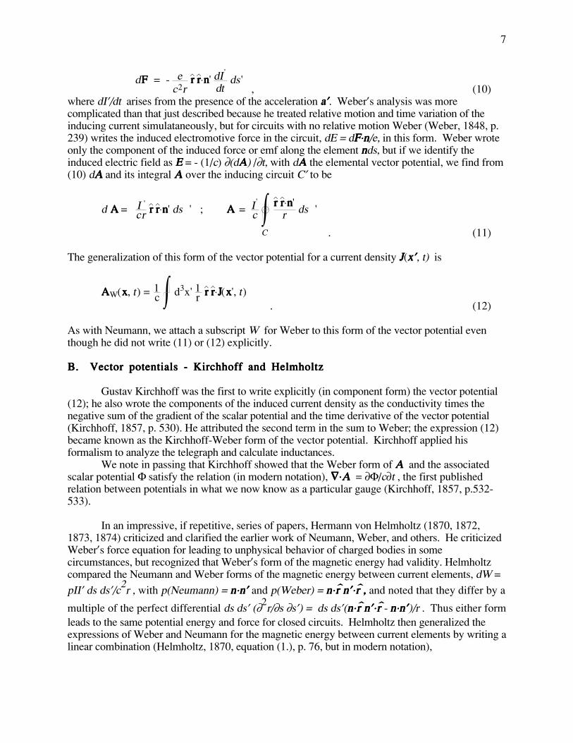
dFFFF = - ec2r

rrrr rrrr°nnnn' dI '

dt ds'

, (10)where dI’/dt arises from the presence of the acceleration aaaa’’’’. Weber’s analysis was morecomplicated than that just described because he treated relative motion and time variation of theinducing current simulataneously, but for circuits with no relative motion Weber (Weber, 1848, p.239) writes the induced electromotive force in the circuit, dE = dFFFF°°°°nnnn/e, in this form. Weber wroteonly the component of the induced force or emf along the element nnnnds, but if we identify theinduced electric field as EEEE = - (1/c) Ç(dAAAA) /Çt, with dAAAA the elemental vector potential, we find from(10) dAAAA and its integral AAAA over the inducing circuit C’ to be

d AAAA = I 'cr rrrr rrrr°nnnn' ds ' ; AAAA = I'

c rrrr rrrr°nnnn'r ds '

C'

. (11)

The generalization of this form of the vector potential for a current density JJJJ(xxxx’’’’, t) is

AAAAW(xxxx, t) = 1c d3x' 1r rrrr rrrr°JJJJ(xxxx', t). (12)

As with Neumann, we attach a subscript W for Weber to this form of the vector potential eventhough he did not write (11) or (12) explicitly.

BBBB.... VVVVeeeeccccttttoooorrrr ppppooootttteeeennnnttttiiiiaaaallllssss ---- KKKKiiiirrrrcccchhhhhhhhooooffffffff aaaannnndddd HHHHeeeellllmmmmhhhhoooollllttttzzzz

Gustav Kirchhoff was the first to write explicitly (in component form) the vector potential(12); he also wrote the components of the induced current density as the conductivity times thenegative sum of the gradient of the scalar potential and the time derivative of the vector potential(Kirchhoff, 1857, p. 530). He attributed the second term in the sum to Weber; the expression (12)became known as the Kirchhoff-Weber form of the vector potential. Kirchhoff applied hisformalism to analyze the telegraph and calculate inductances.

We note in passing that Kirchhoff showed that the Weber form of AAAA and the associatedscalar potential Ï satisfy the relation (in modern notation), àààà°°°°AAAA = ÇÏ/cÇt , the first publishedrelation between potentials in what we now know as a particular gauge (Kirchhoff, 1857, p.532-533).

In an impressive, if repetitive, series of papers, Hermann von Helmholtz (1870, 1872,1873, 1874) criticized and clarified the earlier work of Neumann, Weber, and others. He criticizedWeber’s force equation for leading to unphysical behavior of charged bodies in somecircumstances, but recognized that Weber’s form of the magnetic energy had validity. Helmholtzcompared the Neumann and Weber forms of the magnetic energy between current elements, dW =pII’ ds ds’/c2r , with p(Neumann) = nnnn°°°°nnnn’’’’ and p(Weber) = nnnn°°°°ú úúúrrrr nnnn’’’’°°°°ú úúúrrrr ,,,, and noted that they differ by a

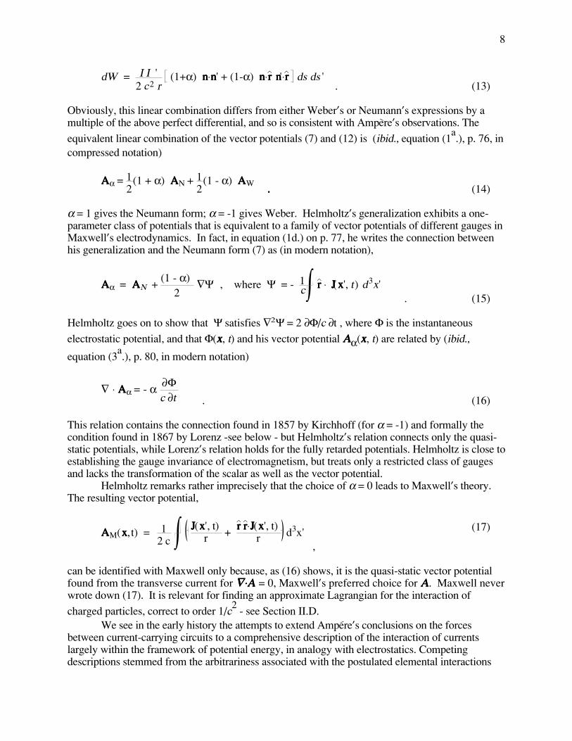
multiple of the perfect differential ds ds’ (Ç2r/Çs Çs’) = ds ds’(nnnn°°°°ú úúúrrrr nnnn’’’’°°°°ú úúúrrrr - nnnn°°°°nnnn’’’’)/r . Thus either formleads to the same potential energy and force for closed circuits. Helmholtz then generalized theexpressions of Weber and Neumann for the magnetic energy between current elements by writing alinear combination (Helmholtz, 1870, equation (1.), p. 76, but in modern notation),

8

dW = I I '2 c2 r

(1+å) nnnn°nnnn' + (1-å) nnnn°rrrr nnnn'°rrrr ds ds ' . (13)

Obviously, this linear combination differs from either Weber’s or Neumann’s expressions by amultiple of the above perfect differential, and so is consistent with Ampere’s observations. Theequivalent linear combination of the vector potentials (7) and (12) is (ibid., equation (1

a.), p. 76, in

compressed notation)

AAAAå = 12

(1 + å) AAAAN + 12

(1 - å) AAAAW .... (14)

å = 1 gives the Neumann form; å = -1 gives Weber. Helmholtz’s generalization exhibits a one-parameter class of potentials that is equivalent to a family of vector potentials of different gauges inMaxwell’s electrodynamics. In fact, in equation (1d.) on p. 77, he writes the connection betweenhis generalization and the Neumann form (7) as (in modern notation),

AAAAå = AAAAN + (1 - å)

2 àÁ , where Á = - 1

c rrrr ° JJJJ(xxxx', t) d3x' . (15)

Helmholtz goes on to show that Á satisfies ◊Á = 2 ÇÏ/c Çt , where Ï is the instantaneouselectrostatic potential, and that Ï(xxxx, t) and his vector potential AAAAå(xxxx, t) are related by (ibid.,

equation (3a.), p. 80, in modern notation)

à ° AAAAå = - å ÇÏc Çt

. (16)

This relation contains the connection found in 1857 by Kirchhoff (for å = -1) and formally thecondition found in 1867 by Lorenz -see below - but Helmholtz’s relation connects only the quasi-static potentials, while Lorenz’s relation holds for the fully retarded potentials. Helmholtz is close toestablishing the gauge invariance of electromagnetism, but treats only a restricted class of gaugesand lacks the transformation of the scalar as well as the vector potential.

Helmholtz remarks rather imprecisely that the choice of å = 0 leads to Maxwell’s theory.The resulting vector potential,

AAAAM(xxxx,t) = 12 c

JJJJ(xxxx', t)

r + rrrr rrrr°JJJJ(xxxx', t)

r d3x' ,

(17)

can be identified with Maxwell only because, as (16) shows, it is the quasi-static vector potentialfound from the transverse current for àààà°°°°AAAA = 0, Maxwell’s preferred choice for AAAA. Maxwell neverwrote down (17). It is relevant for finding an approximate Lagrangian for the interaction ofcharged particles, correct to order 1/c2

- see Section II.D.We see in the early history the attempts to extend Ampere’s conclusions on the forces

between current-carrying circuits to a comprehensive description of the interaction of currentslargely within the framework of potential energy, in analogy with electrostatics. Competingdescriptions stemmed from the arbitrariness associated with the postulated elemental interactions

9

between current elements, an arbitrariness that vanished upon integration over closed circuits.These differences led to different but equivalent forms for the vector potential. The focus was onsteady-state current flow or quasi-static behavior. Meanwhile, others were addressing thepropagation of light and its possible connection with electricity, electric currents, and magnetism.That electricity was due to discrete charges and electric currents to discrete charges in motion was aminority view, Weber being a notable exception. Gradually, those ideas gained credence andcharged particle dynamics came under study. Our story now turns to these developments and howthe concept of different gauges was elaborated, and by whose hands.

CCCC.... EEEElllleeeeccccttttrrrrooooddddyyyynnnnaaaammmmiiiiccccssss bbbbyyyy MMMMaaaaxxxxwwwweeeellllllll,,,, LLLLoooorrrreeeennnnzzzz,,,, aaaannnndddd HHHHeeeerrrrttttzzzz

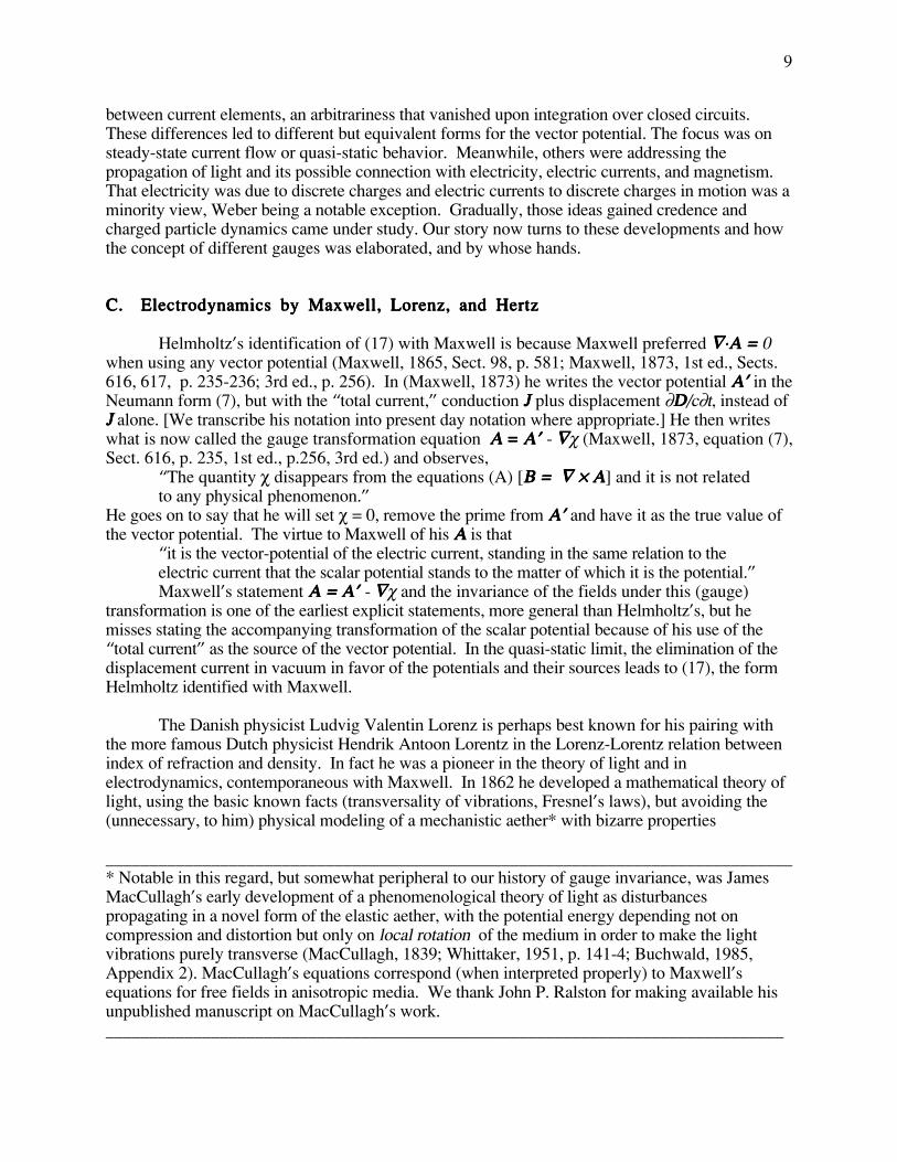
Helmholtz’s identification of (17) with Maxwell is because Maxwell preferred àààà°°°°AAAA ==== 0when using any vector potential (Maxwell, 1865, Sect. 98, p. 581; Maxwell, 1873, 1st ed., Sects.616, 617, p. 235-236; 3rd ed., p. 256). In (Maxwell, 1873) he writes the vector potential AAAA’’’’ in theNeumann form (7), but with the “total current,” conduction JJJJ plus displacement ÇDDDD/cÇt, instead ofJJJJ alone. [We transcribe his notation into present day notation where appropriate.] He then writeswhat is now called the gauge transformation equation AAAA ==== AAAA’’’’ - ààààç (Maxwell, 1873, equation (7),Sect. 616, p. 235, 1st ed., p.256, 3rd ed.) and observes,

“The quantity ç disappears from the equations (A) [BBBB ==== àààà ‡‡‡‡ AAAA] and it is not related to any physical phenomenon.”

He goes on to say that he will set ç = 0, remove the prime from AAAA’’’’ and have it as the true value ofthe vector potential. The virtue to Maxwell of his AAAA is that

“it is the vector-potential of the electric current, standing in the same relation to theelectric current that the scalar potential stands to the matter of which it is the potential.”Maxwell’s statement AAAA ==== AAAA’’’’ - ààààç and the invariance of the fields under this (gauge)

transformation is one of the earliest explicit statements, more general than Helmholtz’s, but hemisses stating the accompanying transformation of the scalar potential because of his use of the“total current” as the source of the vector potential. In the quasi-static limit, the elimination of thedisplacement current in vacuum in favor of the potentials and their sources leads to (17), the formHelmholtz identified with Maxwell.

The Danish physicist Ludvig Valentin Lorenz is perhaps best known for his pairing withthe more famous Dutch physicist Hendrik Antoon Lorentz in the Lorenz-Lorentz relation betweenindex of refraction and density. In fact he was a pioneer in the theory of light and inelectrodynamics, contemporaneous with Maxwell. In 1862 he developed a mathematical theory oflight, using the basic known facts (transversality of vibrations, Fresnel’s laws), but avoiding the(unnecessary, to him) physical modeling of a mechanistic aether* with bizarre properties

______________________________________________________________________________* Notable in this regard, but somewhat peripheral to our history of gauge invariance, was JamesMacCullagh’s early development of a phenomenological theory of light as disturbancespropagating in a novel form of the elastic aether, with the potential energy depending not oncompression and distortion but only on local rotation of the medium in order to make the lightvibrations purely transverse (MacCullagh, 1839; Whittaker, 1951, p. 141-4; Buchwald, 1985,Appendix 2). MacCullagh’s equations correspond (when interpreted properly) to Maxwell’sequations for free fields in anisotropic media. We thank John P. Ralston for making available hisunpublished manuscript on MacCullagh’s work._____________________________________________________________________________

10

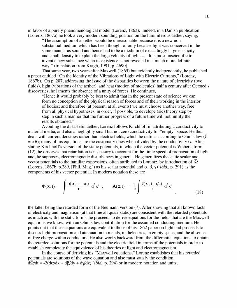
in favor of a purely phenomenological model (Lorenz, 1863). Indeed, in a Danish publication(Lorenz, 1867a) he took a very modern sounding position on the luminiferous aether, saying,

“The assumption of an ether would be unreasonable because it is a new non-substantial medium which has been thought of only because light was conceived in the same manner as sound and hence had to be a medium of exceedingly large elasticity and small density to explain the large velocity of light. ..... It is most unscientific toinvent a new substance when its existence is not revealed in a much more definiteway.” (translation from Kragh, 1991, p. 4690).That same year, two years after Maxwell (1865) but evidently independently, he published

a paper entitled “On the Identity of the Vibrations of Light with Electric Currents,” (Lorenz,1867b). On p. 287, addressing the issue of the disparities between the nature of electricity (twofluids), light (vibrations of the aether), and heat (motion of molecules) half a century after Oersted’sdiscoveries, he laments the absence of a unity of forces. He continues,

“Hence it would probably be best to admit that in the present state of science we can form no conception of the physical reason of forces and of their working in the interior of bodies; and therefore (at present, at all events) we must choose another way, free from all physical hypotheses, in order, if possible, to develope (sic) theory step bystep in such a manner that the further progress of a future time will not nullify theresults obtained.”Avoiding the distasteful aether, Lorenz follows Kirchhoff in attributing a conductivity to

material media, and also a negligibly small but not zero conductivity for “empty” space. He thusdeals with current densities rather than electric fields, which he defines according to Ohm’s law (JJJJ= ßEEEE); many of his equations are the customary ones when divided by the conductivity ß. Afterstating Kirchhoff’s version of the static potentials, in which the vector potential is Weber’s form(12), he observes that retardation is necessary to account for the finite speed of propagation of lightand, he supposes, electromagnetic disturbances in general. He generalizes the static scalar andvector potentials to the familiar expressions, often attributed to Lorentz, by introduction of Æ„(Lorenz, 1867b, p.289, [Phil. Mag.]) as his scalar potential and å, ∫, © ( ibid., p. 291) as thecomponents of his vector potential. In modern notation these are

Ï(xxxx, t) = ®( xxxx', t - r/c)

r d3x' ; AAAA(xxxx,t) = 1 c

JJJJ(xxxx', t - r/c)r d3x'

, (18)

the latter being the retarded form of the Neumann version (7). After showing that all known factsof electricity and magnetism (at that time all quasi-static) are consistent with the retarded potentialsas much as with the static forms, he proceeds to derive equations for the fields that are the Maxwellequations we know, with an Ohm’s law contribution for the assumed conducting medium. Hepoints out that these equations are equivalent to those of his 1862 paper on light and proceeds todiscuss light propagation and attenuation in metals, in dielectrics, in empty space, and the absenceof free charge within conductors. He also works backward from the differential equations to obtainthe retarded solutions for the potentials and the electric field in terms of the potentials in order toestablish completely the equivalence of his theories of light and electromagnetism.

In the course of deriving his “Maxwell equations,” Lorenz establishes that his retardedpotentials are solutions of the wave equation and also must satisfy the condition,dÆ„/dt = -2(då/dx + d∫/dy + d©/dz) (ibid., p. 294) or in modern notation and units,

11

à ° AAAA + 1c ÇÏÇt

= 0 . (19)

This equation, now almost universally called the “Lorentz condition,” is seen to originate withLorenz more than 25 years before Lorentz. In discussing the quasi-static limit, Lorenz remarks (p.292) that the retarded potentials (in modern, corrected terms, the “Lorenz” gauge potentials) givethe same fields as the instantaneous scalar potential and a vector potential that is “a mean betweenWeber’s and Neumann’s theories,” namely, (17), appropriate for Maxwell’s choice of àààà°°°°AAAA = 0.Without explicit reference, Lorenz was apparently aware of and made use of what we call gaugetransformations.

Lorenz’s paper makes no reference to Maxwell. Indeed, he only cites himself, but by 1873Maxwell knew of Lorenz’s paper and in his Treatise, at the end of the chapter giving hiselectromagnetic theory of light, he mentions Lorenz’s work as covering essentially the same ground(Maxwell, 1973, 1st ed., Note after Sect. 805, p. 398; 3rd ed., p. 449-450). Although Lorenz madea number of contributions to optics and electromagnetism during his career (Kragh, 1991, 1992),his pioneering papers were soon forgotten because they were not connected by his contemporarieswith the works of Maxwell, Heaviside, and Hertz. He died in 1891, inadequately recognized thenor later. In fact, by 1900 his name had disappeared from the mainstream literature onelectromagnetism.

The mistaken attribution of (19) to Lorentz was pointed out by O’Rahilly (1938), VanBladel (1991), and others. That Lorenz, not Lorentz, was the father of the retarded potentials (18)was first pointed out by Whittaker (1951, p.268) but he mistakenly states (ibid., p.394) that Levi-Civita was the first to show (in 1897) that potentials defined by these integrals satisfy (19). Levi-Civita in fact does just what Lorenz did in 1867. Lorentz’s own use of the Lorenz condition isdiscussed below.

Heinrich Hertz is most famous for his experiments in the 1880s demonstrating the freepropagation of electromagnetic waves (Hertz, 1892), but he is equally important for histheoretical viewpoint. In 1884, beginning with the quasi-static, instantaneous electric and magneticvector potentials of Helmholtz et al, he developed an iteration scheme that led to wave equations forthe potentials and to the Maxwell equations in free space for the fields (Hertz, 1896, ElectricWaves, p.273-290). His iterative approach showed one path from the action-at-a-distancepotentials to the dynamical Maxwell equations for the fields. Hertz (ibid., p.286) states that both

“Riemann in 1858 and Lorenz in 1867, with a view to associating optical and electrical phenomena with one another, postulated the same or quite similar laws for the propagation of the potentials. These investigators recognized that these laws involve the addition of new terms to the forces which actually occur in electromagnetics; and they justify this by pointing out that these new terms are too small to beexperimentally observable. But we see that the addition of these terms is far from needing any apology. Indeed their absence would necessarily involve contradiction of principles which are quite generally accepted.”

It seems that Hertz did not fully appreciate that, while Lorenz’s path from potentials to fieldequations was different in detail from his, Lorenz accomplished the same result 17 years earlier.Lorenz was not apologizing, but justifying his adoption of the retarded potentials as the necessarygeneralization, still in agreement with the known facts of electricity and magnetism. They were hisstarting point for obtaining his form of the Maxwell equations.

Six years later, Hertz (Hertz, 1892, p.193-268) addressed electrodynamics for bodies at restand in motion. He discussed various applications, with the fields always to the fore and the scalarand vector potentials secondary. In this endeavor he made common cause with Heaviside, to whomhe gives prior credit. Both men believed the potentials were unnecessary and confusing. In

12

calculations Hertz apparently avoided them at all costs; Heaviside used them sparingly (O’Hara andPricha, 1987, p.58, 62, 66-67). By using only the fields, Hertz avoided the issue of different formsof the potentials - his formalism was gauge invariant, by definition*.______________________________________________________________________________

* Hertz did not avoid potentials entirely. His name is associated with the “polarization potentials”of radiation problems.______________________________________________________________________________

DDDD.... CCCChhhhaaaarrrrggggeeeedddd ppppaaaarrrrttttiiiicccclllleeee ddddyyyynnnnaaaammmmiiiiccccssss ---- CCCCllllaaaauuuussssiiiiuuuussss,,,, HHHHeeeeaaaavvvviiiissssiiiiddddeeee,,,, aaaannnndddd LLLLoooorrrreeeennnnttttzzzz ((((1111888899992222))))

We have already described Weber’s force equation (8) for the interaction of chargedparticles. While it permitted Weber to deduce the correct force between closed current-carryingcircuits, it does not even remotely agree to order 1/c2

with the force between two charges inmotion. It also implies inherently unphysical behavior, as shown by Helmholtz (1873). Weber’swork was important nevertheless in its focus on charged particles instead of currents and itsinitiation of the Kirchhoff-Weber form of the vector potential.

A significant variation on charged particle dynamics, closer to the truth than Weber’s, wasproposed by Rudolf Julius Emanuel Clausius (1877, 1880). Struck by Helmholtz’s demonstrationof the equivalence of Weber’s and Neumann’s expressions for the interaction of charges or currentelements, Clausius chose to write Lagrange’s equations with an interaction of two charged particlese and e’ that amounts to an interaction Lagrangian of the form,*______________________________________________________________________________

* Prior to the end of the 19th century in mechanics and the beginning of the 20th century inelectrodynamics the compact notation of L for T - V was rarely used in writing Lagrange’sequations. We use the modern notation Lint as a convenient shorthand despite its absence in thepapers cited.______________________________________________________________________________

Lint = ee 'r -1 + vv

vv°vvvv'c2

..... (20)

Generalized to one charge e interacting with many, treated as continuous charge and currentdensities (®, JJJJ), this Lagrangian reads

Lint = e - Ï(xxxx, t) + 1c vvvv°AAAAN(xxxx, t) , (21)

where Ï is the instantaneous Coulomb potential and AAAAN is the instantaneous Neumann potential(7) with a time-dependent current. The interaction (20), inherent in Neumann’s earlier work oncurrents, is a considerable step forward in the context of charged particle interactions, but itsinstantaneous action-at-a-distance structure means that it is not a true description, even to order1/c2

. (The force deduced from it has the correct magnetic field coupling to order 1/c2, but lacks

some of the corresponding corrections to the electric field contribution.)

13

In an impressive paper, Oliver Heaviside (1889) chose àààà°°°°AAAA = 0 (so that the instantaneousCoulomb field is exact) and constructed the appropriate vector potential, (17) for a point source, togive the velocity-dependent interaction correct to order 1/c2

(Heaviside, 1889, p.328, Eq.(8)). Fortwo charges e and e’ with velocities vvvv and vvvv’’’’, respectively, his results are equivalent to theinteraction Lagrangian,

Lint = e e 'r - 1 + 1

2c2 vvvv°vvvv' + rrrr°vvvv rrrr°vvvv'

. (22)

Heaviside also derived the magnetic part of the Lorentz force. His contributions, like Lorenz’s,were largely ignored subsequently. Darwin (1920) derived (22) by another method with noreference to Heaviside and applied it to problems in the old quantum theory. See also Fock (1959).

A different approach was developed by H. A. Lorentz (1892) as part of hiscomprehensive statement of what we now call the microscopic Maxwell theory, with charges atrest and in motion as the sole sources of electromagnetic fields. His chapter IV is devoted to theforces between charged particles. The development is summarized on p.451-2 by statement of themicroscopic Maxwell equations and the Lorentz force equation, FFFF = e [ EEEE + vvvv ‡‡‡‡ BBBB/c ]. In usingD’Alembert’s principle to derive his equations, Lorentz employs the vector potential, but neverstates explicitly its form in terms of the sources. It is clear, however, that he has retardation inmind, on the one hand from his exhibition of the full Maxwell equations to determine the fieldscaused by his ® and JJJJ = ®vvvv, and on the other by his words at the beginning of the chapter. He callshis reformulation (in translation from the French)

“a fundamental law comparable to those of Weber and Clausius, while maintaining the consequences of Maxwell’s principles.”

A few sentences later, he stresses that the action of one charged particle on another is propagated atthe speed of light, a concept originated by Gauss in 1845, but largely ignored for nearly 50 years.

Joseph Larmor (1900) used the principle of least action for the combined system ofelectromagnetic fields and charged particles to obtain both the Maxwell equations and the Lorentzforce equation. Karl Schwarzschild, later renowned in astrophysics and general relativity,independently used the same technique to discuss the combined system of particles and fields(Schwarzschild, 1903). He was the first to write explicitly the familiar Lagrangian Lint describingthe interaction of a charged particle e , with coordinate xxxx and velocity vvvv, with retarded externalelectromagnetic fields,

Lint = e - Ï(xxxx, t) + 1c vvvv°AAAA(xxxx, t) , (23)

where Ï and AAAA are the potentials (18).It is curious that, to the best of the authors’ knowledge, the issue of gauge invariance of this

charged particle Lagrangian did not receive general consideration in print until 1941 in the text byLandau and Lifshitz (1941). See also Bergmann (1946). The proof is simple. Under the gaugetransformation (1a,b) the Lagrangian (23) is augmented by

ÎLint = e 1c ÇçÇt

+ 1c vvvv°àç = e c dç

dt

, (24)

14

a total time derivative and so makes no contribution to the equations of motion. Perhaps thisobservation is too obvious to warrant publication in other than textbooks. We note that, in derivingthe approximate Lagrangian attributed to him, Darwin (1920) expands the retarded potentials for acharged particle, which involve rrrr = xxxx(t) -xxxx’’’’(t’), in powers of (t’-t) = -r/c , with coefficients of theprimed particle’s velocity, acceleration, etc., to obtain a tentative Lagrangian and then adds a totaltime derivative to obtain (22). Fock (1959) makes the same expansion, but then explicitly makes agauge transformation to arrive at (22). These equivalent procedures exploit the arbitrariness of(24).

EEEE.... LLLLoooorrrreeeennnnttttzzzz:::: tttthhhheeee aaaacccckkkknnnnoooowwwwlllleeeeddddggggeeeedddd aaaauuuutttthhhhoooorrrriiiittttyyyy,,,, ggggeeeennnneeeerrrraaaallll ggggaaaauuuuggggeeee ffffrrrreeeeeeeeddddoooommmm

Our focus here is on how H. A. Lorentz became identified as the originator of both thecondition (19) between Ï and AAAA and the retarded solutions (18). In chapter VI, Lorentz (1892)presents, without attribution, a theorem that the integral

F(xxxx, t) = 14π

1r s(xxxx', t ' = t -r/c) d3x'

(25a)

is a solution of the inhomogeneous wave equation with s(xxxx,,,, t) as a source term,

1c2

Ç2F

Çt 2 - ◊F = s(xxxx, t)

. (25b)

He then uses such retarded solutions for time integrals of the vector potential in a discussion ofdipole radiation.

In fact, the theorem goes back to Riemann in 1858 and Lorenz in 1861 and perhaps others.Riemann apparently read his paper containing the theorem to the Gíottingen academy in 1858, buthis death prevented publication, remedied only in Riemann (1867). In (Lorenz, 1867b), Lorenzstates (25a,b) and remarks that the demonstration is easy, giving as reference his paper on elasticwaves (Lorenz, 1861). It seems clear that in 1861 Lorenz was unaware of Riemann’s oralpresentation. The posthumous publication of Riemann’s note occurred simultaneously with andadjacent to Lorenz’s 1867 paper in Annalen*.

In (Lorentz, 1895, Sect. 32), Lorentz quotes the theorem (25a,b), citing (Lorentz, 1892) forproof, and then in Sect. 33 writes the components of a vector field in the form equivalent to (18)with JJJJ = ®vvvv. He does not call his vector field (¥x , ¥y , ¥z ) the vector potential. Having obtainedthe wave equation for HHHH with àààà ‡‡‡‡ JJJJ as source term, he merely notes that if HHHH is defined as the curlof his vector field, it is sufficient that the field satisfy the wave equation with JJJJ as source. We thussee Lorentz in 1895 explicitly exhibiting retarded solutions, but without the condition (19).

______________________________________________________________________________

* Riemann (1867) showed that retardation led to the quasi-static instantaneous interactions ofWeber and Kirchhoff, much as done by Lorentz (1867b), and remarked on the connection betweenthe velocity of propagation of light and the ratio of electrostatic and electromagnetic units.______________________________________________________________________________

15

In a festschrift volume in honor of the 25th anniversary of Lorentz’s doctorate, EmilWiechert (1900) summarizes the history of the wave equation and its retarded solutions. Hecites Riemann in1858, Poincare in 1891, Lorentz (1892, 1895), and Levi-Civita in 1897. Nomention of Lorenz! In the same volume, des Coudres (1900) cites (Lorentz, 1892) for thetheorem (25a,b) and calls the retarded solutions (18) “Lorentz’schen Líosungen.” It is evident thatby 1900 the physics community had attributed the retarded solutions for Ï and AAAA to Lorentz, tothe exclusion of others.

Additional reasons for Lorentz being the reference point for modern classicalelectromagnetism are his magisterial encyclopedia articles (Lorentz, 1904a, 1904b), and his book(Lorentz, 1909). Here we find the first clear statement of the arbitrariness of the potentials underwhat we now call general gauge transformations. On p. 157 of (Lorentz, 1904b), he first statesthat in order to have the potentials satisfy the ordinary wave equations they must be related by

à° AAAA = - 1c ÇÏÇt

. [Lorentz’s (2)].

He then discusses the arbitrariness in the potentials, stating that other potentials AAAA0 and Ï0 maygive the same fields, but not satisfy his constraint. He then states “every other admissible pair AAAAand Ï “ can be related to the first pair via the transformations,

AAAA = AAAA0 - àç , Ï = Ï0 + 1c ç . (26)

He then says that the scalar function ç can be found so that AAAA and Ï do satisfy [Lorentz’s (2)] bysolving the inhomogeneous wave equation,

׍ - 1c2

ç = à°AAAA0 + 1c Ï0 . (27)

A reader might question whether Lorentz was here stating the general principle of what weterm gauge invariance. He stated his constraint before his statement of the arbitrariness of thepotentials and then immediately restricted ç to a solution of (27). This doubt is removed in his book(Lorentz, 1909). There, in Note 5, he says,

“Understanding by AAAA0 and Ï0 special values, we may represent other values thatmay as well be chosen by [our equation (26)] where ç is some scalar function (emphasisadded). We shall determine ç by subjecting AAAA and Ï to the condition [Lorentz’s (2)] whichcan always be fulfilled because it leads to the equation [our equation (27)] which can besatisfied by a proper choice of ç.”

He then proceeds to the wave equations and the retarded solutions in Sect. 13 of the main text.Lorentz obviously preferred potentials satisfying his constraint to the exclusion of other choices,but he did recognize the general principle of gauge invariance in classical electromagnetism withoutputting stress on it.

The dominance of Lorentz’s publications as source documents is illustrated by their citationby G. A. Schott in his Adams Prize essay (Schott, 1912). On p. 4, Schott quotes (19) [hisequation (IX)] and the wave equations for AAAA and Ï. He then cites Lorentz’s second Encyclopediaarticle (Lorentz, 1904b) and his book (Lorentz, 1909) for the retarded solutions (18) [his equations(X) and (XI)], which he later on the page calls “the Lorentz integrals.”

16

Lorentz’s domination aside, the last third of the 19th century saw the fundamentals ofelectromagnetism almost completely clarified, with the aether soon to disappear. Scientists wentabout applying the subject with confidence. They did not focus on niceties such as the arbitrarinessof the potentials, content to follow Lorentz in use of the retarded potentials (18). It was only withthe advent of modern quantum field theory and the construction of the electroweak theory andquantum chromodynamics that the deep significance of gauge invariance emerged.

IIIIIIIIIIII.... DDDDAAAAWWWWNNNNIIIINNNNGGGG OOOOFFFF TTTTHHHHEEEE QQQQUUUUAAAANNNNTTTTUUUUMMMM EEEERRRRAAAA

AAAA.... 1111999922226666 :::: SSSScccchhhhrrrrí íííooooddddiiiinnnnggggeeeerrrr,,,, KKKKlllleeeeiiiinnnn,,,, FFFFoooocccckkkk

The year 1926 saw the flood gates open. Quantum mechanics, or more precisely, wavemechanics, blossomed at the hands of Erwin Schríodinger and many others. Among the myriadcontributions, we focus only on those that relate to our story of the emergence of the principle ofgauge invariance in quantum theory. The pace among this restricted set is frantic enough. [Todocument the pace, we augment the references for the papers in this era with submission andpublication dates.] The thread we pursue is the relativistic wave equation for spinless chargedparticles, popularly known nowadays as the Klein-Gordon equation. The presence of both thescalar and vector potentials brought forth the discovery of the combined transformations (1 a,b,c)by Fock.

The relativistic wave equation for a spinless particle with charge e interacting withelectromagnetic fields is derived in current textbooks by first transforming the classical constraintequation for a particle of 4-momentum pµ

= (p0, pppp) and mass m , pµpµ = (mc)2, by the substitution

pµ™ pµ

- eAµ/c, where Aµ

= (A0 = Ï, AAAA) is the 4-vector electromagnetic potential. Here we use

the metric g00 = 1, gij

= - ∂ij . Then a quantum mechanical operator acting on a wave function ¥ is

constructed by the operator substitution, pµ ™ iÓǵ

, where ǵ=Ç/Çxµ = (Ç0

, - àààà). Explicitly, wehave

( iÓǵ - eA µ/c )( iÓǵ - eAµ/c ) ¥ = (mc)2 ¥ . (28)

Alternatively, we divide through by -Ó2

and write

(ǵ + ie A µ/Óc )( ǵ + ie Aµ/Óc ) + (mc/Ó)2 ¥ = 0 . (29)

Separation of the space and time dimensions and choice of a constant energy solution,¥ ‚ exp(-iEt/Ó), yields the relativistic version of the Schríodinger equation,

- Ó2c2 ◊¥ +ieÓc(ǵAµ)¥ + 2ieÓc AAAA°à¥ + e 2 AAAA°AAAA ¥ = (E - eÏ)2 - (mc2)2 ¥ . (30)

The second term on the left is absent if the Lorenz gauge condition ǵAµ = 0 is chosen for thepotentials.

The first of Schríodinger’s four papers (Schríodinger, 1926a) was submitted on 27 Januaryand published on 13 March. It was devoted largely to the nonrelativistic time-independent wave

17

equation and simple potential problems, but in Section 3 he mentions the results of his study of the“relativistic Kepler problem.” (An English translation of Schríodinger’s 1926 papers can be foundin (Schríodinger, 1978)). Schríodinger had obviously written down and solved the relativisitc waveequation with a Coulomb potential and had not obtained the Sommerfeld fine-structure formula. Hemust have been disappointed at the disagreement, but in Sect. 6 of his fourth paper (Schríodinger,1926b), he tentatively presented the relativistic equation in detail and discussed its application to thehydrogen atom and to the Zeeman effect.

Schríodinger was not the only person to consider the relativistic wave equation. Oskar Klein(1926) treated a five-dimensional relativistic formalism and explicitly exhibited the four-dimensional relativistic wave equation for fixed energy with a static scalar potential. He showedthat the nonrelativistic limit was the time-independent Schríodinger equation, but did not discussany solutions. Before publication of Klein’s paper, Fock (1926a) independently derived therelativistic wave equation from a variational principle and solved the relativistic Kepler problem.He observed that Schríodinger had already commented on the solution in his first paper. In hispaper Fock did not include the general electromagnetic interaction. Schríodinger comments in theintroduction (“Abstract”) to his collected papers (Schríodinger, 1978),

“V. Fock carried out the calculations quite independently in Leningrad, before my last paper [(Schríodinger, 1926b)] was sent in, and also succeeded in deriving the relativistic equation from a variational principle. Zeitschrift f_íur Physik 33338888, 242 (1926).”The discovery of the symmetry under gauge transformations (1 a,b,c) of the quantum

mechanical system of a charged particle interacting with electromagnetic fields is due to Fock(1926b). His paper was submitted on 30 July 1926 and published on 2 October 1926. In it he firstdiscussed the special-relativistic wave equation of his earlier paper with electromagneticinteractions and addressed the effect of the change in the potentials (1 a,b). He showed that theequation is invariant under the change in the potentials provided the wave function is transformedaccording to (1c). He went on to treat a five-dimensional general-relativistic formalism, similar tobut independent of Klein. In a note added in proof, Fock notes that

“While this note was in proof, the beautiful work of Oskar Klein [published on 10 July]arrived in Leningrad,”

and that the principal results were identical. That fall others contributed. Kudar (1926) wrote therelativistic equations down in covariant notation, citing Klein (1926) and Fock (1926a). Heremarked that his general equation reduced to Fock’s for the Kepler problem with the appropriatechoice of potentials. Walter Gordon (1926) discussed the Compton effect using the relativisticwave equation to describe the scattering of light by a charged particle. He referred to Schríodinger’sfirst three papers, but not the fourth (Schríodinger, 1926b) in which Schríodinger actually treats therelativistic equation. Gordon does not cite Klein or either of Fock’s papers.

The above paragraphs show the rapid pace of 1926, the occasional duplication, and the caretaken by some, but not all, for proper acknowledgment of prior work by others. If we gochronologically by publication dates, the Klein-Gordon equation should be known as the Klein-Fock-Schríodinger equation. Totally apart from the name attached to the relativistic wave equation,the important point in our story is Fock’s paper on the gauge invariance, published on 2 October1926 (Fock, 1926b).

The tale now proceeds to the enshrinement by Weyl of symmetry under gaugetransformations as a guiding principle for the construction of a quantum theory of matter(electromagnetism and gravity). Along the way, we retell the well-known story of how theseemingly inappropriate word “gauge” came to be associated with the transformations(1 a,b,c) and today’s generalizations.

18

BBBB.... WWWWeeeeyyyyllll:::: ggggaaaauuuuggggeeee iiiinnnnvvvvaaaarrrriiiiaaaannnncccceeee aaaassss aaaa bbbbaaaassssiiiicccc pppprrrriiiinnnncccciiiipppplllleeee

Fritz London, in a short note in early 1927 (London, 1927a) and soon after in a longerpaper (London, 1927b), proposed a quantum mechanical interpretation of Weyl’s failed attempt tounify electromagnetism and gravitation (Weyl, 1919). This attempt was undertaken long before thediscovery of quantum mechanics. London noticed that Weyl’s principle of invariance of his theoryunder a scale change of the metric tensor gµó™ gµóexp ¬(x) , where ¬(x) is an arbitrary functionof the space-time coordinates, was equivalent in quantum mechanics to the invariance of the waveequation under the transformations (1) provided ¬(x) was made imaginary. In his short noteLondon cites Fock (1926b) but does not repeat the citation in his longer paper, although he doesmention (without references) both Klein and Fock for the relativistic wave equation in fivedimensions.

To understand London’s point we note first that Weyl’s incremental change of length scaled… = … ƒódxó

leads to a formal solution … = …0exp¬(x), where ¬(x) = âxƒódxó

; the indefinite

integral over the real “potential” ƒó is path-dependent. If we return to the relativistic wave equation(29), we observe that a formal solution for a particle interacting with the electromagnetic potentialAµ

can be written in terms of the solution without interaction as

¥ = exp - i eÓc

Aódxóx

¥ 0 , (31)

where ¥0 is the zero-field solution. [Recovery of (29) may be accomplished by “solving” for ¥0and requiring ǵǵ¥0 + (mc/Ó)2¥0 = 0.] With the gauge transformation of the 4-vector potential

A µ ™ A' µ = Aµ - ǵç , (32)

the difference in phase factors is obviously the integral of a perfect differential, -ǵçdxµ . Up to a

constant phase, the wave functions ¥’ and ¥ are thus related by the phase transformation

¥' = exp(ieç( x)/Óc) ¥ , (33)

which is precisely Fock’s (1c). London actually expressed his argument in terms of “scalechange” … = …0 exp(i¬(x)), where i¬(x) is the quantity in the exponential in (31), and wrote ¥/… =

¥0/…0.The “gradient invariance” of Fock became identified by London and then by Weyl with an

analogue of Weyl’s “eichinvarianz” (scale invariance), even though the former concerns a localphase change and the latter a coordinate scale change. In his famous book, “Gruppentheorie undQuantenmechanik” (Weyl, 1928), Weyl discusses the coupling of a relativistic charged particlewith the electromagnetic field. He observes, without references, that the electromagnetic equationsand the relativistic Schríodinger equation (28) are invariant under the transformations (1a,b,c). Weylthen states on p. 88 (in translation):

19

”This ‘principle of gauge invariance’ is quite analogous to that previously set up by the author, on speculative grounds, in order to arrive at a unified theory of gravitation and electricity

22. But I now believe that this gauge invariance does not tie together

electricity and gravitation, but rather electricity and matter in the manner described above.”

His note 22 refers to his own work, to Schríodinger (1923), and to London (1927b). In the first(1928) edition, the next sentence reads (again in translation):

”How gravitation according to general relativity must be incorporated is not certain at present.”

By the second (1931) edition, this sentence has disappeared, undoubtedly because he believed thathis own work in the meantime (Weyl, 1929a, 1929b) had shown the connection. In fact, in thesecond edition a new section 6 appears in Chapter IV, in which Weyl elaborates on how the gaugetransformation (1c) can only be fully understood in the context of general relativity.

Weyl’s 1928 book and his papers in 1929 demonstrate an evolving point of view unique tohim. Presumably prompted by London’s observation, he addressed the issue of gauge invariancein relativistic quantum mechanics, knowing on the one hand that the principle obviously applied tothe electromagnetic fields and charged matter waves, and on the other hand wanting to establishcontact with his 1919 “eichinvarianz.” As we have just seen, in his 1928 book he presented theidea of gauge invariance in the unadorned version of Fock, without the “benefit” of generalrelativity. But in the introduction of the first of his 1929 papers on the electron and gravitation(Weyl, 1929a), he states the “principle of gauge invariance” (the first use of the words in English)very much as in his book, citing only it for authority. He then goes on to show that theconservation of electricity is a double consequence of gauge invariance and that

“This new principle of gauge invariance ..... has the character of general relativity since it contains an arbitrary function ¬, and can certainly only be understood with reference to it.”

His (incorrect) insistence on the support of general relativity in order that the gauge function be anarbitrary function of the space-time coordinates stems from his belief that in special relativity thevalue of ¬ at one space-time point is related to its value at another point by a pure Lorentztransformation and, being a Lorentz scalar, is constant everywhere. In Weyl’s view, only in generalrelativity with curved space-time can one have a different arbitrary phase at every point.

Despite his insistence on the need of general relativity to understand fully the concept ofgauge invariance, Weyl stated ( Weyl, 1929a, p.332, below equation (8)),

“If our view is correct, then the electromagnetic field is a necessary accompaniment of the matter wave field and not of gravitation.”

The last sentence of (Weyl, 1929b) contains almost the same words. His viewpoint about the needfor general relativity can perhaps be understood in the sense that ¬ must be an arbitrary function inthe curved space-time of general relativity, but not necessarily in special relativity, and his desire toprovide continuity with his earlier work.

Historically, of course, Weyl’s 1929 papers were a watershed. They enshrined asfundamental the modern principle of gauge invariance, in which the existence of the 4-vectorpotentials (and field strengths) follow from the requirement of the invariance of the matterequations under gauge transformations such as (1c) of the matter fields. This principle is thetouchstone of the theory of gauge fields, so dominant in theoretical physics in the second half ofthe 20th century. The important developments beyond 1929 can be found in the reviews alreadymentioned in the Introduction. The reader should be warned, however, of a curiosity regarding thecitation of Fock’s 1926 paper (Fock, 1926b) by O’Raifeartaigh (1997), O’Raifeartaigh andStraumann (2000), and Yang (1986. 1987). While the volume and page number are givencorrectly, the year is invariably given as 1927. One of the writers privately blames it on Pauli

20

(1933). Indeed, Pauli made that error, but he did give to Fock the priority of introducing gaugeinvariance in quantum theory.

IIIIVVVV.... PPPPHHHHYYYYSSSSIIIICCCCAAAALLLL MMMMEEEEAAAANNNNIIIINNNNGGGG OOOOFFFF GGGGAAAAUUUUGGGGEEEE IIIINNNNVVVVAAAARRRRIIIIAAAANNNNCCCCEEEE,,,, EEEEXXXXAAAAMMMMPPPPLLLLEEEESSSS

AAAA.... OOOOnnnn tttthhhheeee pppphhhhyyyyssssiiiiccccaaaallll mmmmeeeeaaaannnniiiinnnngggg ooooffff ggggaaaauuuuggggeeee iiiinnnnvvvvaaaarrrriiiiaaaannnncccceeee iiiinnnn QQQQEEEEDDDD aaaannnndddd qqqquuuuaaaannnnttttuuuummmm mmmmeeeecccchhhhaaaannnniiiiccccssss

While for Electroweak Theory and QCD gauge invariance is of paramount importance, itsphysical meaning in QED per se does not seem to be extremely profound. A tiny mass of thephoton would destroy the gauge invariance of QED, as a mass term m©

2 A2

in the Lagrangian isnot gauge invariant. At the same time the excellent agreement of QED with experiment and inparticular its renormalizability would not be impaired (see e.g., Kobzarev and Okun, 1968;Goldhaber and Nieto, 1971). On the other hand the renormalizability would be destroyed by ananomalous magnetic moment term in the Lagrangian, µÆ¥ß¬ó¥F¬ó

, in spite of its manifest gaugeinvariance. What is really fundamental in electrodynamics is the conservation of electromagneticcurrent or in other words conservation of charge (see e.g. Okun, 1982; Okun, 1986, Lecture 1).Conservation of charge makes the effects caused by a possible nonvanishing mass of the photon,m© , proportional to m©

2 and therefore negligibly small for small enough values of m© .

It should be stressed that the existing upper limits on the value of m© lead in the case ofnon-conserved current to such catastrophic bremsstrahlung, that most of the experiments whichsearch for monochromatic photons in charge-nonconserving processes become irrelevant (Okunand Zeldovich, 1978). Further study has shown (Voloshin and Okun, 1978) that reabsorption ofvirtual bremsstrahlung photons restores the conservation of charge (for reviews, see Okun, 1989a,1989b, 1992).

As has been already stressed above, gauge invariance is a manifestation of non-observability of A

µ. However integrals such as in eq (31) are observable when they are taken over

a closed path, as in the Aharonov-Bohm effect (Aharonov and Bohm, 1959). The loop integral ofthe vector potential there can be converted by Stokes’s theorem into the magnetic flux through theloop, showing that the result is expressible in terms of the magnetic field, albeit in a nonlocalmanner. It is a matter of choice whether one wishes to stress the field or the potential, but the localvector potential is not an observable.

BBBB.... EEEExxxxaaaammmmpppplllleeeessss ooooffff ggggaaaauuuuggggeeeessss

The gauge invariance of classical field theory and of electrodynamics in particular allows toconsider the potential Aµ

with various gauge conditions, most of them being not Poincareinvariant:

ǵAµ = 0 (µ = 0,1, 2, 3) , Lorenz gauge (34)

àààà°°°°AAAA = ÇjAj = 0 (j = 1, 2, 3) , Coulomb gauge or radiation gauge (35)

nµAµ= 0 (n2

= 0) , light cone gauge (36)

21

Ao = 0 , Hamiltonian or temporal gauge (37)

A3 = 0 , axial gauge (38)

xµAµ

=0 , Fock-Schwinger gauge (39)

xjAj = 0 , Poincare gauge (40)

An appropriate choice of gauge simplifies calculations. This is illustrated by many examplespresented in textbooks, e.g., (Jackson, 1998). For the quantum mechanics of nonrelativisticcharged particles interacting with radiation, the Coulomb gauge is particularly convenient becausethe instantaneous scalar potential describing the static interactions and binding is unquantized; onlythe transverse vector potential of the photons is quantized. However, noncovariant gauges, charac-terized by fixing a direction in Minkowski space, pose a number of problems discussed in Gaig,Kummer, and Schweda (1990). The problems acquire additional dimensions in quantum fieldtheory where one has to deal with a space of states and with a set of operators.

In QED the gauge degree of freedom has to be fixed before the theory is quantized.Usually the gauge fixing term (ǵA

µ)2 is added to the gauge invariant Lagrangian density with

coefficient 1/2å (For futher details see Gaig, Kummer, and Schweda, 1990; Berestetskii, Lifshitz,and Pitaevskii, 1971; Ramond, 1981; Zinn-Justin, 1993). In perturbation theory the propagator of avirtual photon with 4-momentum k acquires the form,

D(k)µó = - 1k2

gµó + ( å - 1)kµkó

k2

. (41)

The most frequently used cases are

å = 1 ( Feynman gauge), (42)

å = 0 (Landau gauge). (43)

In Feynman gauge the propagator (41) is simpler, while in the Landau gauge its longitudinal partvanishes, which is often more convenient. If calculations are carried out correctly, the final resultwill not contain the gauge parameter å.

In the static (zero frequency) limit the propagator (41) reduces to

D i j(kkkk, 0) = 1|kkkk|2

∂i j + (å - 1)ki kj

|kkkk|2

, (44)D 0 0(kkkk, 0) = 1

|kkkk|2

, (45)

D 0j(kkkk, 0) = D i 0(kkkk, 0) = 0 . (46)This is the propagator for the Helmholtz potential (14) and the static Coulomb potential.

22

Various gauges have been associated with names of physicists, a process begun by Heitlerwho introduced the term “Lorentz relation” in the first edition of his book (Heitler, 1936). In thethird edition (Heitler, 1954) he used “Lorentz gauge” and “Coulomb gauge.” Zumino (1960)introduced the terms “Feynman gauge,” “Landau gauge,” and “Yennie gauge” (å = 3).

VVVV.... SSSSUUUUMMMMMMMMAAAARRRRYYYY AAAANNNNDDDD CCCCOOOONNNNCCCCLLLLUUUUDDDDIIIINNNNGGGG RRRREEEEMMMMAAAARRRRKKKKSSSS

What is now generally known as a gauge transformation of the electromagnetic potentials(1a, b) was discovered in the process of formulation of classical electrodynamics by its creators,Lorenz, Maxwell, Helmholtz, and Lorentz, among others (1867-1909). The phase transformation(1c) of the quantum mechanical charged field accompanying the transformation of theelectromagnetic potentials was discovered by Fock (1926b). The term “gauge” was applied to thistransformation by Weyl ( 1929a, 1929b) (who used “eich-” a decade before to denote a scaletransformation in his unsuccessful attempt to unify gravity and electromagnetism).

In text books on classical electrodynamics the gauge invariance (1a,b) was first discussedby Lorentz in his influential book, “Theory of Electrons” (Lorentz, 1909). The first derivation ofthe invariance of the Lagrangian for the combined system of electromagnetic fields and chargedparticles was presented by Landau and Lifshitz (1941) (with reference to Fock, they used Fock'sterm "gradient invariance"). The first model of a non-abelian gauge theory of weak, strong, and electromagneticinteractions was proposed by Klein (1938) (who did not use the term "gauge” and did not refer toWeyl). But this attempt was firmly forgotten. The modern era of gauge theories started with thepaper by Yang and Mills (1954).

The history of gauge invariance resembles a random walk, with the roles of some importantearly players strangely diminished with time. There is a kind of echo between the loss of interestby O. Klein and L. Lorenz in their "god blessed children". It is striking that the notion of gaugesymmetry did not appear in the context of classical electrodynamics, but required the invention ofquantum mechanics. It is amusing how little the authors of text-books know about the history ofphysics. For a further reading the Resource Letter (Cheng and Li, 1988) is recommended.

AAAACCCCKKKKNNNNOOOOWWWWLLLLEEEEDDDDGGGGEEEEMMMMEEEENNNNTTTTSSSS

The authors thank Robert N. Cahn, David J. Griffiths, Helge Kragh, and Valentin L.Telegdi for their assistance and advice. The work of JDJ was supported in part by the Director,Office of Science, Office of High Energy and Nuclear Physics, of the U.S. Department of Energyunder Contract DE-AC03-76SF00098. The work of LBO was supported in part by grant RFBR #00-15-96562, by an Alexander von Humboldt award, and by the Theory Division, CERN.

23

RRRREEEEFFFFEEEERRRREEEENNNNCCCCEEEESSSS

Aharonov, Y., and D. Bohm, 1959, “Significance of Electromagnetic Potentials in the Quantum Theory,” Phys. Rev. 111111115555, 485-491.

Ampere, A.-M., 1827, “Sur la theorie mathematique des phenomens electrodynamiques uniquement deduite de l’experience,” Memoires de l’Academie Royale des Sciences de l’Institut de France, ser. 2, 6666, 175-388 [memoirs presented from 1820 to 1825].

Berestetskii, V. B., E. M. Lifshitz, and L. P. Pitaevskii, 1971, Relativistic Quantum Theory,Part 1 ( Pergamon, Oxford), Section 77.

Bergmann, P. G., 1946, Introduction to the Theory of Relativity (Prentice-Hall, New York),p.115-117.

Biot, J. B., and F. Savart, 1820, “Experiences electro-magnetiques,” Journal de Phys., de Chimie, 99991111, 151; “Note sur le Magnetisme de la pile de Volta,” Ann. de Chimieet de Phys, ser. 2, 11115555,,,, 222-223.

Biot, J. B., 1824, Precis Elementaire de Physique Experimentale, 3rd ed., vol 2 (Deterville,Paris), p. 745.

Buchwald, J. Z., 1985, From Maxwell to Microphysics (University of Chicago Press, Chicago)

Buchwald, J. Z., 1989, The Rise of the Wave Theory of Light (University of Chicago Press, Chicago)

Buchwald, J. D., 1994,The Creation of Scientific Effects, Heinrich Hertz and Electric Waves(University of Chicago Press, Chicago)

Cheng, T. P., and Ling-Fong Li, 1988, "Resource Letter: GI-1 Gauge invariance," Am. J. Phys. 55556666, 586-600.

Clausius, R., 1877, “Ueber die Ableitung eines neuen elektrodynamischen Grundgestezes,” Journal fíur Math. (Crelle’s Journal) 88882222, 85-130.

Clausius, R., 1880, “On the employment of the electrodynamic potential for the determination of the ponderomotive and electromotive forces,” Phil. Mag., ser. 5, 11110000, 255-279

des Coudres, Th., 1900, “Zur Theorie des Kraftfeldes elektrischer Ladungen, die sich mit Ueberlichtgeschwindigkeit Bewegen,” Arch. Neerl. Scs., ser. 2, 5555, 652-664.

Darwin, C. G., 1920, “The Dynamical Motions of Charged particles,” Phil. Mag., ser. 6, 33339999, 537-551.

Faraday, M., 1939, Experimental Researches in Electricity, Vol. 1 (Richard & John EdwardTaylor, London), p.1-41. [from Phil. Trans. Roy. Soc., November 24, 1831]

24

Fock, V., 1926a, “Zur Schríodingerschen Wellenmechanik,” Zeit. fíur Phys. 33338888, 242-250.[subm. 11 June 1926, publ. 28 July 1926]

Fock, V., 1926b, "ùUber die invariante Form der Wellen- und der Bewegungsgleichungen fíur einen geladenen Massenpunkt," Zeit. fííur Physik 33339999, 226-232.[subm. 30 July 1926, publ. 2 October 1926]

Fock, V., 1959, Theory of Space, Time and Gravitation, transl. M. Hamermesh, (PergamonPress, London), 2nd ed. (1965), Sect. 26.

Gaig, P., W. Kummer, and M. Schweda, 1990, Eds., Physical and Nonstandard Gauges, Proceedings of a Workshop, Vienna, Austria (September 19-23, 1989), Lecture Notes in Physics, 361 (Springer-Verlag, Berlin-Heidelberg).

Grassmann, H., 1845, “Neue Theorie der Electrodynamik,” Ann. der Phys. und Chem., 66664444,1-18.

Goldhaber, A. S., and M. M. Nieto, 1971, "Terrestrial and extraterrestrial limits on photon mass," Rev. Mod. Phys. 44443333, 277-296.

Gordon, W., 1926, “Der Comptoneffekt nach der Schríodingerschen Theorie,” Zeit. fíur Phys. 44440000, 117-133. [subm, 29 September 1926, publ. 29 November 1926]

Heaviside, O., 1889, “On the Electromagnetic Effects due to the Motion of Electrification through a Dielectric,” Phil. Mag. ser. 5, 22227777, 324-339.

Heitler, W., 1936, Quantum Theory of Radiation, 1st ed.(Oxford University Press)

Heitler, W., 1954, Quantum Theory of Radiation, 3rd ed.(Oxford University Press)

Helmholtz, H., 1870, “Ueber die Bewegungsgleichungen der Elektricitíat fíur ruhende leitende Kíorper,” Journal fíur die reine und angewandte Mathematik 77772222, 57-129.

Helmholtz, H., 1872, “On the Theory of Electrodynamics,” Phil. Mag. ser. 4, 44444444, 530-537.

Helmholtz, H., 1873, “Ueber die Theorie der Elektrodynamik,” Journal fíur die reine und angewandte Mathematik 77775555, 35-66.[called Zweite Abhandlung Kritisches]

Helmholtz, H., 1874, “Ueber die Theorie der Elektrodynamik,” Journal fíur die reine und angewandte Mathematik 77778888, 273-324.[called the Dritte Abhandlung, andsubtitled “Die elektrodynamischen Kríafte in bewegten Leitern.”]

Hertz, H., 1892, Untersuchungen ueber die Ausbreitung der elektrischen Kraft (J. A. Barth, Leipzig); transl., Electric Waves, Auth. English translation by D. E. Jones (Macmillan,London, 1893; reprinted, Dover Publications, New York, 1962)

Hertz, H., 1896, Miscellaneous Papers, Auth. English translation by D. E. Jones and G. A. Schott (Macmillan, London).

25

Jackson, J. D., 1998, Classical Electrodynamics, 3rd ed. (Wiley, New York)

Jelved, K., A. D. Jackson, and O. Knudsen, 1998, Transl. & Eds., Selected Scientific Works of Hans Christian Oersted (Princeton University Press), p. 413-420.

Kirchhoff, G., 1857, “II. Ueber die Bewegung der Elektricitíat in Leitern,” Annalen der Physik und Chemie 111100002222, 529-544. [reprinted in Gesammelte Abhandlungen von G. Kirchhoff (J. A. Barth, Leipzig 1882), p. 154-168]

Klein, O., 1926, “Quantentheorie und fíunfdimensionale Relativitíatstheorie,” Zeit. fíur Phys. 33337777, 895-906. [subm. 28 April 1926, publ. 10 July 1926]

Klein, O., 1938, “On the Theory of Charged Fields,” in New Theories in Physics, Conference organized in collaboration with the International Union of Physics and the Polish Intellectual Cooperation Committee (Warsaw, May 30th- June 3rd, 1938).

Kobzarev, I. Yu., and L. B. Okun, 1968, "On the photon mass,” Usp. Fiz. Nauk 99995555, 131-137[Sov. Phys. Uspekhi 11111111, 338-341.]

Kragh, H., 1991, “Ludvig Lorenz and nineteenth century optical theory: the work of a great Danish scientist,” Appl. Optics 33330000, 4688-4695.

Kragh, H., 1992, “Ludvig Lorenz and the Early Theory of Long-distance Telephony,” Centaurus 33335555, 305-324.

Kudar, J., 1926, “Zur vierdimensionale Formulierung der undulatorischen Mechanik,” Ann. der Physik 88881111, 632-636. [subm. 30 August 1926, publ. 26 October 1926]

Landau, L. D., and E. M. Lifshitz, 1941, Teoria Polya, GITTL M.-L., Sect. 16; transl.,Classical Theory of Fields, rev. 2nd ed. (Pergamon Press, Oxford 1962), Sect. 18.

Larmor J., 1900, Aether and Matter (Cambridge University Press), Ch. VI, esp. Sects. 56-58.

London, F., 1927a, “Die Theorie von Weyl und die Quantenmechanik,” Naturwiss. 11115555, 187. [subm. 19 January 1927, publ. 25 February 1927]

London, F., 1927b, “Quantenmechanische Deutung der Theorie von Weyl,” Zeit. fíur Physik 44442222, 375-389. [subm. 25 February 1927; publ. 14 April 1927]

Lorentz, H. A., 1892, “La theorie electromagnetique de Maxwell et son application aux corps mouvants,” Arch. Neerl. Scs. 22225555, 363-552.

Lorentz, H. A., 1895, Versuch einer Theorie der Electrischen und Optischen Erscheinungen in begwegten Kíorpern ( E. J. Brill, Leiden).

Lorentz, H. A., 1904a, Encykl. Math. Wissen., Band V:2, Heft 1, V. 13, “Maxwell’s Elektromagnetische Theorie,” p. 63-144.

26

Lorentz, H. A., 1904b, ibid., V. 14, “Weiterbildung der Maxwellischen Theorie. Elektronentheorie,” p. 145-280.

Lorentz, H. A., 1909, Theory of Electrons (G. B. Teubner, Leipzig and G. E. Stechert, New York).[2nd ed., 1916; reprinted by Dover Publications, New York. 1952]

Lorenz, L. V., 1861, “Memoire sur la theorie de l’elasticite des corps homogenes a elasticite constante,” J. fíur Math. (Crelle’s Journal) 55558888, 329-351.

Lorenz, L. V., 1863, “Die Theorie des Lichtes, I,” Annalen der Physik und Chemie 11118888, 111-145; “On the Theory of Light,” Phil. Mag. ser. 4, 22226666, 81-93, 205-219.

Lorenz, L. V., 1867a, “Om lyset,” Tidsckr. Fys. Chem. 6666, 1-9.

Lorenz, L. V., 1867b, “Ueber die Identitíat der Schwingungen des Lichts mit den elektrischen Stríomen,” Ann. der Physik und Chemie 111133331111, 243-263; “On the Identity of the Vibrations of Light with Electrical Currents, ”Phil. Mag. ser. 4, 33334444, 287-301.

MacCullagh, J., 1839, “Dynamical Theory of crystalline Reflexion and Refraction,” Proc. Roy. Irish Acad. 1111, No,. 20, 374-379; Trans. Roy. Irish Acad. 22221111, part 1, 17-50 (1846); Collected Works of James MacCullagh, eds. J. H. Jellet and S. Haughton (Hodges,Figgis, Dublin, 1880). p.145 - 184.

Maxwell, J. C., 1865, “A Dynamical Theory of the Electromagnetic Field,” Phil. Trans. Roy. Soc. CCCCLLLLVVVV (1865); Scientific Papers (Dover reprint), Vol. 1, p. 526-597. [Part VI is on the electromagnetic theory of light.]

Maxwell, J. C., 1873, Treatise on Electricity and Magnetism, 1st ed. (Clarendon Press, Oxford), Vol. II [3rd edition, 1891, Dover Publications, New York, 1954]

Neumann, F. E., 1847, “Allgemeine Gesetze der inducirten elektriche Stríome,” Abhandlungen derKíoniglichen Akademie der Wissenschaften zu Berlin, aus dem Jahre 1845, 1-87.

Neumann, F. E., 1849, “ùUber ein allgemeines Princip der mathematischen Theorie inducirter elektricher Stríome,” Abhandlungen der Kíoniglichen Akademie der Wissenschaften zu Berlin, aus dem Jahre 1847, 1-72.

Novozhilov, Y. V., and V. Y. Novozhilov, 1999, “Works of Vladimir Aleksandrovich Fock in quantum field theory (On the centennial of the birth of V. A. Fock),” Teor. Mat. Fiz. 111122220000, 400-416 [Theor. Math. Phys 111122220000, 1150-1163].

Novozhilov, Y. V., and V. Y. Novozhilov, 2000, “Vladimir A. Fock (dedicated to the 100th anniversary of birth of academician V.A. Fock),” Fiz. Elem. Cha. Atom. Yad. 33331111, 5-46. [Phys. Part. Nucl. 33331111, 1-21].

O’Hara, J. G. and W. Pricha, 1987, Hertz and the Maxwellians (Peter Peregrinus,London)

27

Okun, L. B., and Ya. B. Zeldovich, 1978, "Paradoxes of unstable electron," Phys. Lett. 77778888BBBB,597-599.

Okun, L. B., 1982, Leptons and Quarks (North-Holland, Amsterdam).

Okun, L. B., 1986, "Special topics on gauge theories," Surveys in High Energy Physics 5555, no.3,Five lectures 199-235, Supplement 236-285. [Originally published in 1983 JINR-CERN School of Physics, Tabor, Czechoslovakia, 5-18 June 1983, vol. 2 (Dubna 1984),pp.2-81.]

Okun, L. B., 1989a, "Tests of electric charge conservation and the Pauli principle,” Usp. Fiz. Nauk 111155558888, 293-301. [Sov. Phys. Uspekhi 33332222, 543-547].

Okun, L. B., 1989b, "Comments on testing charge conservation and the Pauli exclusion principle", Comments Nucl. Part. Phys. 11119999, 99-117.

Okun, L. B., 1992, "Note on testing charge conservation and the Pauli exclusion principle," Phys. Rev. D 44445555, No.11, part II, VI-10 - VI.14.

O’Rahilly, A., 1938, Electromagnetics (Longmans, Green and Cork University Press),reprinted as Electromagnetic Theory (Dover Publications, N.Y. 1965), footnote, p.184.

O’Raifeartaigh, L., 1997, The Dawning of Gauge Theory (Princeton University Press, Princeton, NJ). [A reprint volume with commentary].

O’Raifeartaigh, L., and N. Straumann, 2000, “Gauge theory: Historical origins and somemodern developments,” Rev. Mod. Phys. 77772222, 1-23.

Pauli, W., 1933, in H. Geiger and K. Scheel, Handbuch der Physik, Vol. XXIV/1,Quantentheorie (Springer, Berlin), p. 111, footnote1; transl., W. Pauli, General Principles of Quantum Mechanics, Springer, Berlin (1980), p. 30, footnote 9.

Pihl, M., 1939, Der Physiker L. V. Lorenz: Eine Kritische Untersuchung (Munksgaard, Copenhagen).

Pihl, M., 1972, “The scientific achievements of L.V. Lorenz,” Centaurus 11117777, 83-94.

Prokhorov, L. V., 2000, “V. A. Fock - The Density of Some Discoveries,” Fiz. Elem. Cha. Atom. Yad. 33331111, 47-70 [Phys. Part. Nucl. 33331111, 22-33].

Ramond, P., 1981, Field Theory, A Modern Primer (Benjamin/Cummings, Reading, Mass.), Chapters VII and VIII.

Reiff, R., and A. Sommerfeld, 1902, "Standpunkt der Fernwirkung die Elementargesetze," Encykl.Math. Wissen., Band V:2, V. 12, 1-62.

Riemann, B., 1867, “Ein Beitrag zur Elektrodynamik,” Ann. der Physik und Chemie 111133331111,237-243); “A Contribution to Electrodynamics,” Phil. Mag. ser. 4, 33334444, 368-372.

28

Schott, G. A., 1912, Electromagnetic Radiation (Cambridge University Press).

Schríodinger, E., 1923, “ùUber eine bemerkenswerte Eigenschaft der Quantenbahnen eines einzelnen Elektrons,” Zeit. fíur Physik 11112222, 13-23.

Schríodinger, E., 1926a, “Quantisierung als Eigenwertproblem I,” Ann. der Physik 77779999, 361-376. [subm. 27 January 1926, publ. 13 March 1926]

Schríodinger, E., 1926b, “Quantisierung als Eigenwertproblem IV,” Ann. der Physik 88881111, 109-139. [subm. 21 June 1926, publ. 8 September 1926]

Schríodinger, E., 1978, “Collected Papers on Wave Mechanics,” transl. from 2ndGerman ed., 1928 (Chelsea Publishing, N.Y.).

Schwarzschild, K., 1903, “Zur Elektrodynamik I. Zwei Formen des Princips der kleinstenAction in der Elektronentheorie,” Gott. Nach., Math.-phys. Kl., 126-131.

Van Bladel, J., 1991, “Lorenz or Lorentz?,” IEEE Antennas and Propagation Magazine 33333333, No. 2, 69.

Voloshin, M. B., and L. B. Okun, 1978, "Conservation of electric charge,” Pis’ma Zh. Eksp. Teor. Fiz. 22228888, 156-160. [JETP Lett. 22228888, 145-149]

Weber, W., 1878, Elektrodynamische Maassbestimmungen (WeidmannscheBuchhandlung, Leipzig) [A collection of 7 papers, with the same main title, but differing sub-titles, dating from 1846 to 1878. The first part, p. 1-170, is from Abhandlungen der Kíoniglichen Síachsischen Gesellschaft der Wissenschaften, Leipzig (1846)]

Weber, W., 1848, “I. Elektrodynamische Maassbestimmungen,” Annalen der Physik undChemie 77773333, 193-240 [shortened version of the 1846 paper published in theAbhandlungen der Kíoniglichen Síachsischen Gesellschaft der Wissenschaften, Leipzig]

Weyl, H., 1919, “Eine neue Erweiterung der Relativitíatstheorie,” Ann. der Physik 55559999,,,, 101-133.

Weyl, H., 1928, Gruppentheorie und Quantenmechanik (S. Hirzel, Leipzig), p.87- 88;Theory of Groups and Quantum Mechanics, 2nd ed. (1931), transl.H. P. Robertson, Dover, N.Y. (1950), p.100-101.

Weyl, H., 1929a, "Gravitation and the electron," Proc. Nat. Acad. Sci. 11115555, 323-334.[subm. 7 March 1929; publ. 15 April 1929] This paper is an early version inEnglish of Weyl (1929b).

Weyl, H., 1929b, "Elektron und Gravitation," Zeit. fíur Physik 55556666, 330-352.[subm. 8 May 1929; publ. 19 July 1929]

29

Whittaker, E. T., 1951, History of the Theories of Aether and Electricity, The Classical Theories (Philosophical Library, New York).

Wiechert, E., 1900, “Elektrodynamische Elementargestze,” Arch. Neerl. Scs., ser. 2, 5555, 549-573.

Yang, C. N., and R. L. Mills, 1954, "Conservation of isotopic spin and isospin gauge invariance," Phys. Rev. 99996666, 191-195.

Yang, C. N., 1986, “Hermann Weyl’s Contributions to Physics,” in Hermann Weyl, 1885- 1985,ed. K. Chandrasekharan (Springer Verlag, Berlin), p. 7-21.

Yang, C. N., 1987, “Square root of minus one, complex phases, and Erwin Schríodinger,” in Schríodinger : centenary celebration of a polymath, ed. C.W. Kilmister (Cambridge University Press, London), p. 53-64.

Zinn-Justin, J., 1993, Quantum Field Theory and Critical Phenomena (Oxford UniversityPress), Chapter 18.

Zumino, B., 1960, “Gauge Properties of Propagators in Quantum Electrodynamics,” J. Math. Phys. 1111, 1-7.

FFFFiiiigggguuuurrrreeee CCCCaaaappppttttiiiioooonnnn

Figure 1. Two closed current carrying circuits C and C’ with currents I and I’, respectively

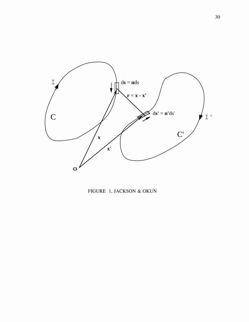
30

C

C'

r = x - x'

O

x

x'

ds = nds

ds' = n'ds'

I

I'

FIGURE 1, JACKSON & OKUN