History and applications of molecular dynamics

•  Fermi-Pasta-Ulam (Chapter 9.3)

Statistical mechanics<-->molecular dynamics

•  Ergodic theorem

System explores all possible states and can effectively attain thermal equilbrium

•  Equipartition of energy

In a harmonic system, E=kT per mode. Violated in FPU problem

A classic paper… establishing the field

Only 864 atoms! Today we can approach even billions!

More modern work with MD… highly interdisciplinary

•  Physics, materials science, chemistry, chemical engineering and even mechanical engineering groups use MD

•  Physics groups at UCF using MD at some level

1.  Rahman. Surface science, catalysis, chemical reactions

2.  Stolbov. Surface science, catalysis, chemical reactions 3.  Kara. Surface science, dynamics, surface vibrations 4.  Bhattacharya. DNA, polymer transport 5.  Schelling. Thermal and phonon transport, surface

science, diffusino, point-defects and optical properties

Challenges of MD simulation

•  Potential not always understood well--- many body interactions •  Quantum mechanics can be used, but very costly •  Times scales usually at most nanoseconds •  Length scales usually at most several nanometers

Long length and time scales relevant for many applications and experiments are extremely hard to access For example, even just a 10nm radius nanoparticle of say gold atoms requires over 200,000 atoms! Much much more (by at least 3 orders of magnitude) than can be handled with quantum mechanics… not to mention time scales….

!

! F

i= m

i

d2! r i

dt2

MD simulation

Integrate to obtain !

!

! r

i(t)

!

! F

i= m

i

d2! r i

dt2

Is that all there is to it?

Simulation can in some sense be regarded as intermediate between experiment and theory

•  Need a model for forces, interactions

•  Provides a test of theoretical predictions

•  Comparison to experiment tests models and theory

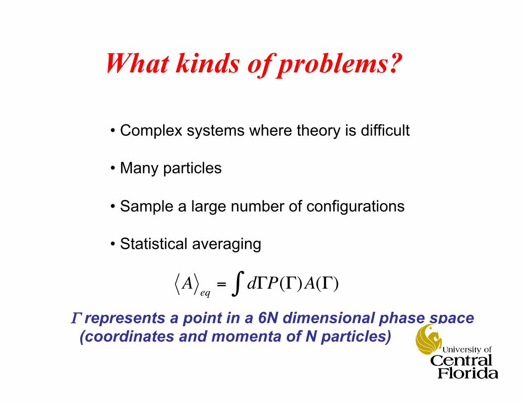
What kinds of problems?

•  Complex systems where theory is difficult

•  Many particles

•  Sample a large number of configurations

•  Statistical averaging

!

Aeq

= d"P(")A(")#Γ represents a point in a 6N dimensional phase space (coordinates and momenta of N particles)

•  Classical dynamics result in Γ(t)

•  Time averages can be made instead of ensemble averages

Connection to molecular dynamics

!

Atime

=1

tA("(t '))dt'

0

t

#

If averaging time is long enough the system should have time to sample the phase space and then,

!

Atime

" Aeq

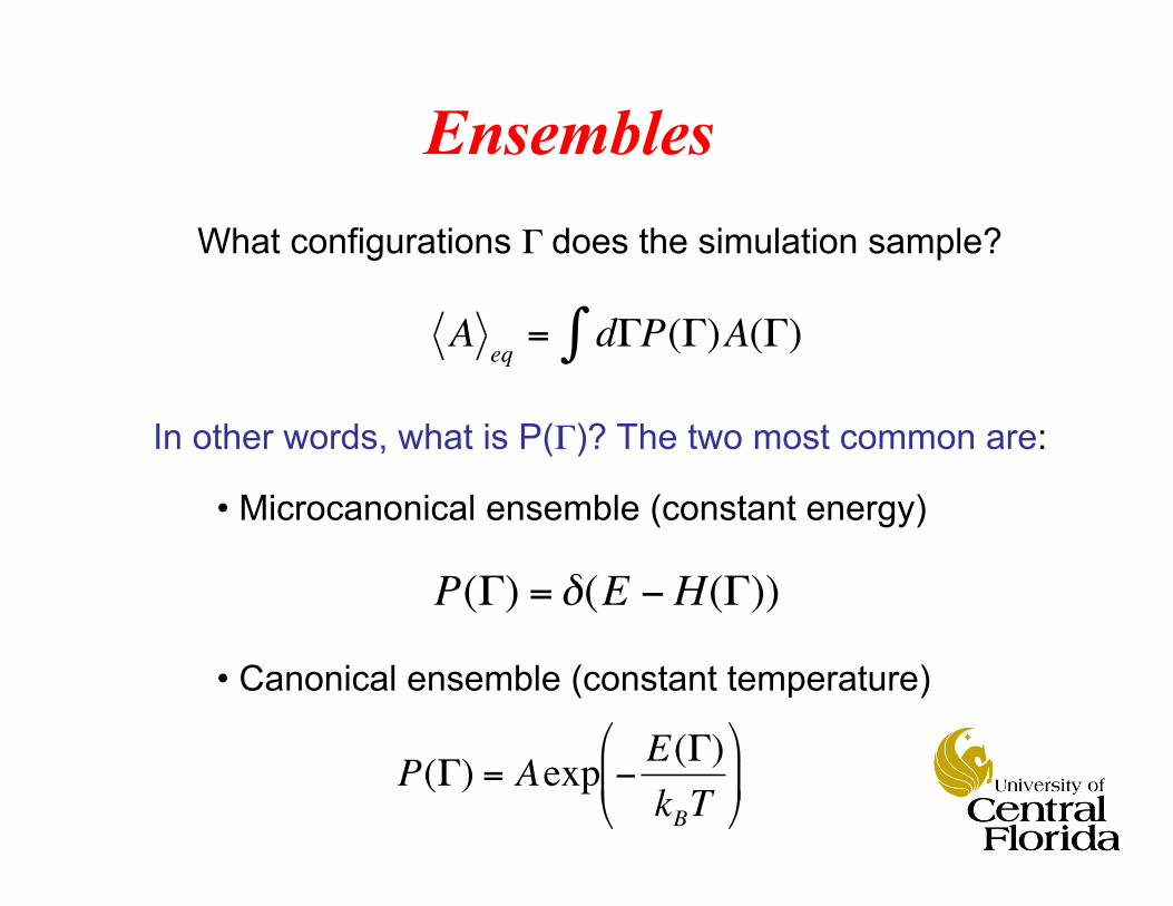
Ensembles

!

Aeq

= d"P(")A(")#

What configurations Γ does the simulation sample?

In other words, what is P(Γ)? The two most common are:

•  Microcanonical ensemble (constant energy)

•  Canonical ensemble (constant temperature)

!

P(") = #(E $H("))

!

P(") = Aexp #E(")

kBT

$

% &

'

( )

!

! F

i= m

i

d2! r

i

dt2

!

d2! r i

dt2"

! r i(t + #t) $ 2

! r i(t) +

! r i(t $#t)

#t2

!

! r

i(t + "t) = 2

! r

i(t) #! r

i(t #"t) +

"t2

mi

! F

i(t)

Verlet Algorithm: numerical integration

More complicated methods like the Gear predictor- corrector algorithm exist, but Verlet works pretty well

Electronic timescales 10-16-10-12s

Molecular-Dynamics Timestep 10-15-10-14s Optical phonon 10-14-10-13s Molecular vibrations in H2O 10-12s Total MD simulation time 10-12-10-6s Long wavelength phonon (sound wave) 10-4-10-1s Chemical reaction (rare event) 10-12-100s

Time Scales Relevant to Materials Simulation

MD timestep must be shorter than characteristic vibrational periods. But total time accessible to MD is often less than interesting problems need!

Diameter of Nucleus 10-13-10-12cm Hydrogen atom ~10-8cm Cesium atom ~2.7x10-8cm Lattice parameter in a crystal 10-8-10-7cm MD simulation cell 10-8-10-4cm Size of a “nanoparticle” 10-7-10-5cm Electronic transistor 10-5cm Grains in a polycrystal 10-4-10-2cm

Length Scales Relevant to Materials Simulation

Molecular dynamics on an atomic scale. Relating to problems on experimental length scales hard!

!

u(rij ) = 4"#

rij

$

% & &

'

( ) )

12

*#

rij

$

% & &

'

( ) )

6+

,

- -

.

/

0 0

Pair Potentials

Lennard-Jones

!

u(rij ) = "Aij

rij6

+ Bij exp("Cijrij ) Buckingham

!

u(rij ) =QiQj

rij

Coulomb

!

U =1

2u(rij

i" j

N

# ) Potential energy sum of pair interactions

Many-Body Potentials

Examples: •  Embedded atom method (metals)

•  Tersoff potentials for covalent bonded crystals

Potential energy not found by summation of pair interactions!

•  Important in metallic and covalent materials

•  Bond strengths depend on number of bonds

•  Energy may depend on directionality of bonds

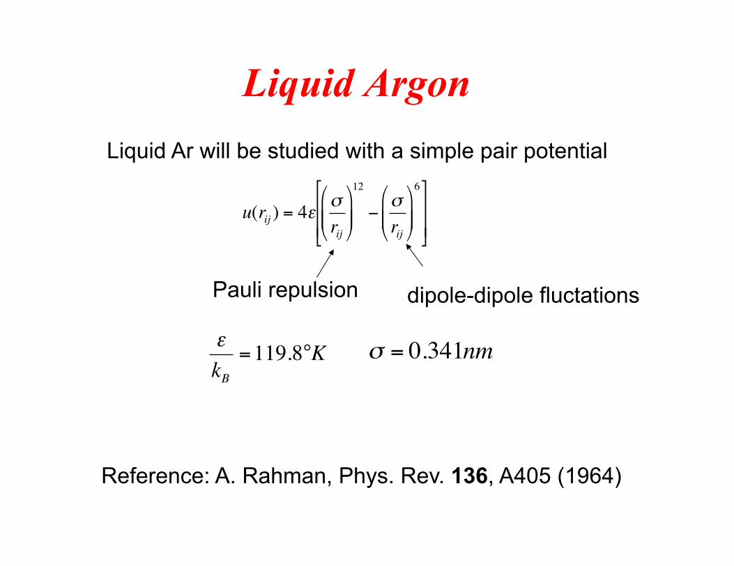
Liquid Argon Liquid Ar will be studied with a simple pair potential

Reference: A. Rahman, Phys. Rev. 136, A405 (1964)

!

u(rij ) = 4"#

rij

$

% & &

'

( ) )

12

*#

rij

$

% & &

'

( ) )

6+

,

- -

.

/

0 0

dipole-dipole fluctations Pauli repulsion

!

"

kB

=119.8°K

!

" = 0.341nm

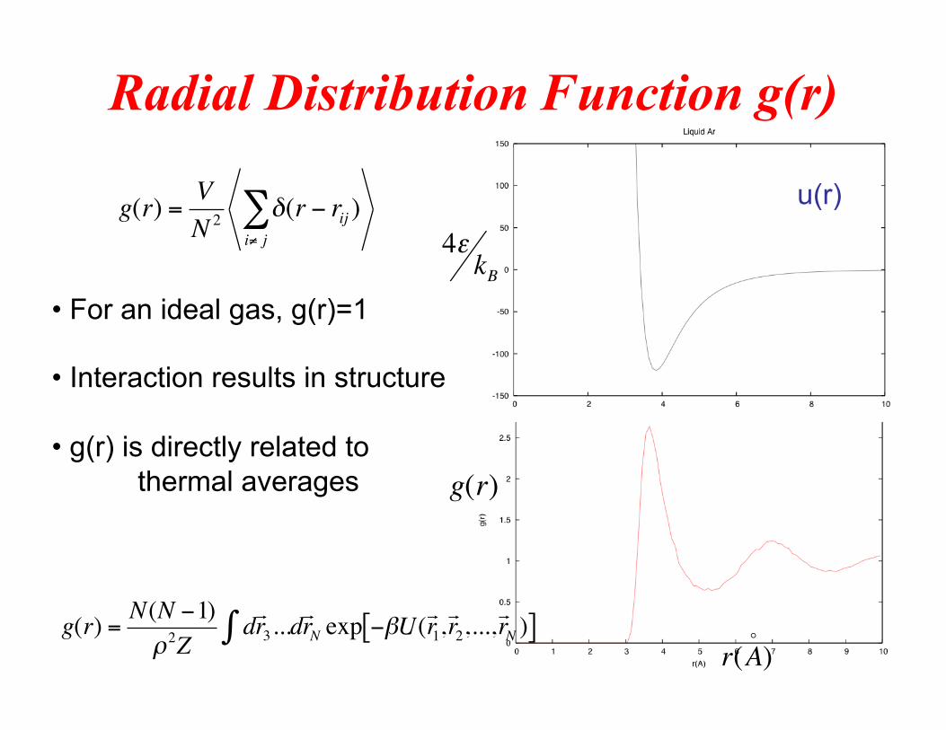
Radial Distribution Function g(r)

•  For an ideal gas, g(r)=1

•  Interaction results in structure

•  g(r) is directly related to thermal averages

!

4"kB

!

g(r)

!

r(A!

)

!

g(r) =N(N "1)

#2Zd! r 3$ ...d! r N exp "%U(

! r 1,! r 2,...,

! r N )[ ]

u(r)

!

g(r) =V

N2

"(r # riji$ j

% )

Diffusion Two Different Ways Einstein Relation:

Linear Response Theory

!

6D" =! r (" ) #

! r (0)

2

!

D =1

3

! v (") #

! v (0)

0

$

% d"

Connection between these evident from,

!

! r (t) "

! r (0) =

! v ( # t )0

t

$ d # t

Some Other Important Examples Ionic Conductivity

Thermal Conductivity

!

" =V

3kBT

! j (#)! j (0)

0

$

% d#

!

" =V

kBT2

! j Q (# )

! j Q (0)

0

$

% d#

Solid Argon •  Argon can be arranged in an fcc, hcp, or bcc lattice •  In an fcc lattice at low temperature, g(r) shows sharp peaks •  Lattice vibrations around equilibrium positions, no diffusion

Radial Distribution Function g(r)

•  Lower temperature, higher pressure •  Positions correlated far away

•  Sharp peaks in Xray scattering

!

4"kB

!

g(r)

!

r(A!

)

!

g(r) =N(N "1)

#2Zd! r 3$ ...d! r N exp "%U(

! r 1,! r 2,...,

! r N )[ ]

u(r)

!

g(r) =V

N2

"(r # riji$ j

% )

Velocity Autocorrelation Function and Spectra

•  Atoms diffusion in our MD crystal will be non existent

•  Fourier transform of Z(τ) gives phonon spectra

•  If vibrations periodic with one frequency ω0,

•  Fourier transform picks out all of the important modes

!

Z(") =1

Ni=1

N

#! v

i(") $! v

i(0)

!

! v

i(") #! v

i(0) = v

i

2(0) exp(i$0")

•  Fluctuations in an MD simulation are important

Example: Fluctuations in total energy E in the canonical ensemble given by, It turns out that this is directly related to the heat capacity

!

"E2

= E2

NVT

# ENVT

2

!

CV

!

CV

=d E

dT=

1

kBT2

E2" E

2[ ]

Fluctuations and Their Significance

•  Remember that in statistical physics,

•  Remember that this is related to the partition function

•  Note that we can also write as,

•  Finally the heat capacity can be found from,

!

E =TrEe

"#E

Tre"#E

!

Z = Tre"#E

!

E

!

E = "#Z

#$=TrEe

"$E

Tre"$E

!

CV

=d E

dT= "

1

kBT2

d E

d#=

1

kBT2

TrE2e"#E

Tre"#E

"TrEe

"#E

Tre"#E

$

% &

'

( )

2*

+ , ,

-

. / /

!

CV

=d E

dT=

1

kBT2

E2" E

2[ ]

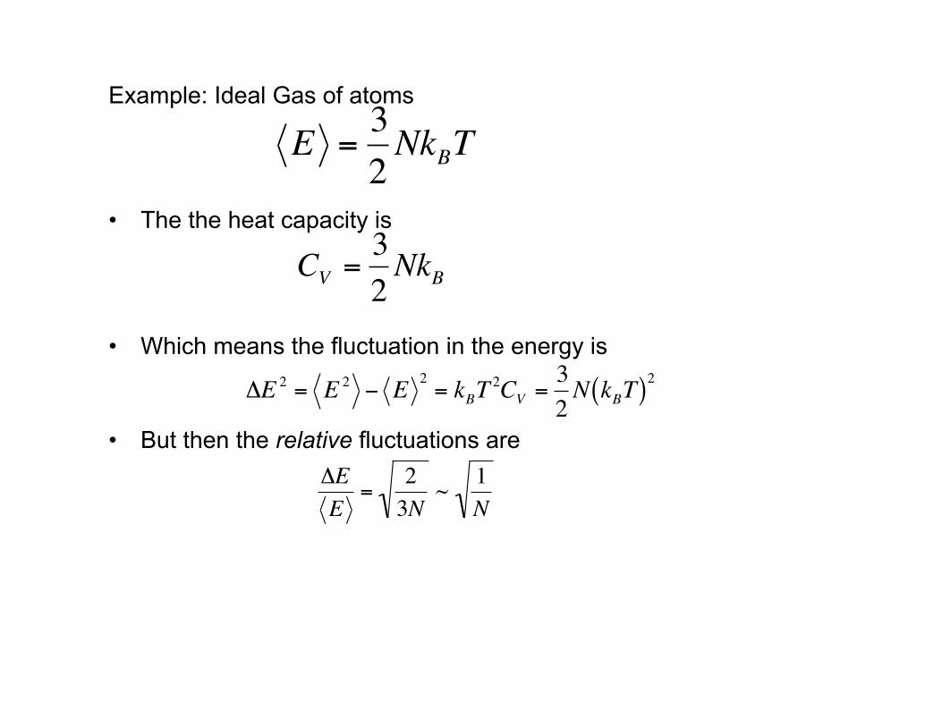
Example: Ideal Gas of atoms

•  The the heat capacity is

•  Which means the fluctuation in the energy is

•  But then the relative fluctuations are

!

E =3

2Nk

BT

!

CV

=3

2Nk

B

!

"E2 = E

2# E

2

= kBT2CV

=3

2N k

BT( )

2

!

"E

E=

2

3N~

1

N

Some good references…

1.  “Computer Simulation of Liquids”, Allen and Tildesley

2.  “The Art of Molecular Dynamics Simulation”, Rapaport

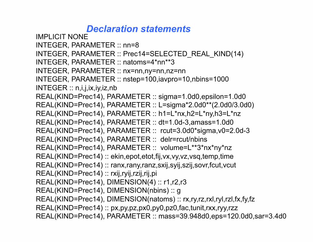
Declaration statements IMPLICIT NONE INTEGER, PARAMETER :: nn=8 INTEGER, PARAMETER :: Prec14=SELECTED_REAL_KIND(14) INTEGER, PARAMETER :: natoms=4*nn**3 INTEGER, PARAMETER :: nx=nn,ny=nn,nz=nn INTEGER, PARAMETER :: nstep=100,iavpro=10,nbins=1000 INTEGER :: n,i,j,ix,iy,iz,nb REAL(KIND=Prec14), PARAMETER :: sigma=1.0d0,epsilon=1.0d0 REAL(KIND=Prec14), PARAMETER :: L=sigma*2.0d0**(2.0d0/3.0d0) REAL(KIND=Prec14), PARAMETER :: h1=L*nx,h2=L*ny,h3=L*nz REAL(KIND=Prec14), PARAMETER :: dt=1.0d-3,amass=1.0d0 REAL(KIND=Prec14), PARAMETER :: rcut=3.0d0*sigma,v0=2.0d-3 REAL(KIND=Prec14), PARAMETER :: delr=rcut/nbins REAL(KIND=Prec14), PARAMETER :: volume=L**3*nx*ny*nz REAL(KIND=Prec14) :: ekin,epot,etot,fij,vx,vy,vz,vsq,temp,time REAL(KIND=Prec14) :: ranx,rany,ranz,sxij,syij,szij,sovr,fcut,vcut REAL(KIND=Prec14) :: rxij,ryij,rzij,rij,pi REAL(KIND=Prec14), DIMENSION(4) :: r1,r2,r3 REAL(KIND=Prec14), DIMENSION(nbins) :: g REAL(KIND=Prec14), DIMENSION(natoms) :: rx,ry,rz,rxl,ryl,rzl,fx,fy,fz REAL(KIND=Prec14) :: px,py,pz,px0,py0,pz0,fac,tunit,rxx,ryy,rzz REAL(KIND=Prec14), PARAMETER :: mass=39.948d0,eps=120.0d0,sar=3.4d0

Time step in picoseconds

! Define the effective time unit in ps fac=10.0d0/(1.381d0*6.022d0) tunit=dsqrt(mass*sar**2*fac/eps) write(6,*) 'tunit=',tunit

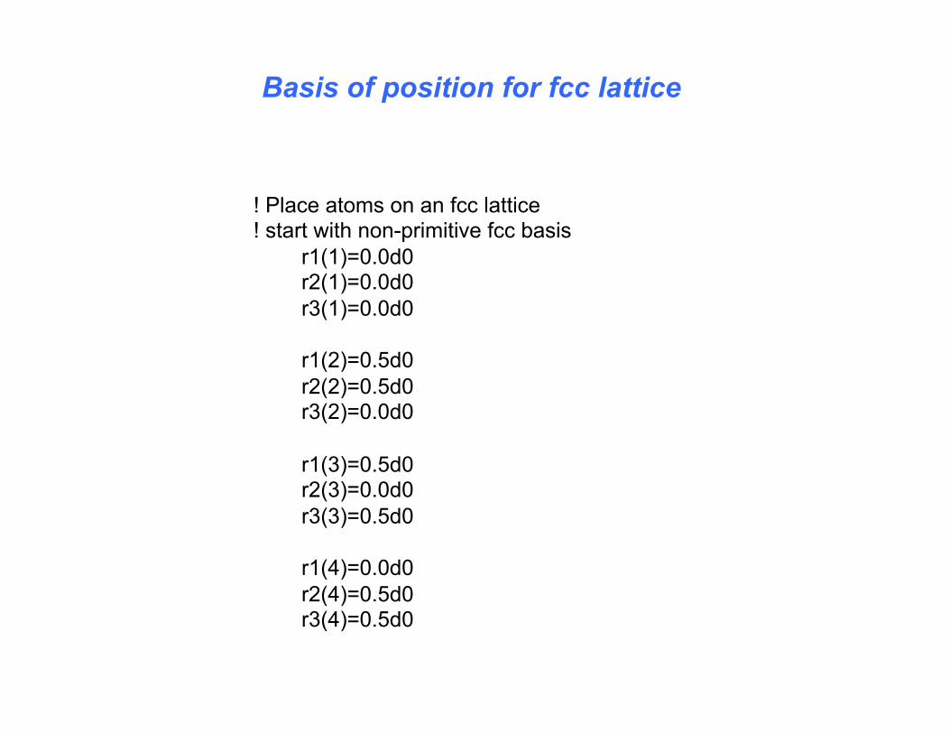
Basis of position for fcc lattice

! Place atoms on an fcc lattice ! start with non-primitive fcc basis r1(1)=0.0d0 r2(1)=0.0d0 r3(1)=0.0d0 r1(2)=0.5d0 r2(2)=0.5d0 r3(2)=0.0d0 r1(3)=0.5d0 r2(3)=0.0d0 r3(3)=0.5d0 r1(4)=0.0d0 r2(4)=0.5d0 r3(4)=0.5d0

Define starting fcc lattice

! now construct lattice n=0 do ix=1,nx do iy=1,ny do iz=1,nz do i=1,4 n=n+1 rx(n)=(r1(i)+dble(ix-1))*sigma ry(n)=(r2(i)+dble(iy-1))*sigma rz(n)=(r3(i)+dble(iz-1))*sigma enddo enddo enddo enddo ! Scale the lattice by desired length L rx=rx*L; ry=ry*L; rz=rz*L

Initial random velocity

! Initialize velocities by picking last position px=0.0d0 ; py=0.0d0 ; pz=0.0d0 call RANDOM_SEED do n=1,natoms call RANDOM_NUMBER(ranx) call RANDOM_NUMBER(rany) call RANDOM_NUMBER(ranz) rxl(n)=rx(n)+v0*(0.5d0-ranx) ryl(n)=ry(n)+v0*(0.5d0-rany) rzl(n)=rz(n)+v0*(0.5d0-ranz) px=px+rx(n)-rxl(n) py=py+ry(n)-ryl(n) pz=pz+rz(n)-rzl(n) enddo write(6,*) 'total momentum px,py,pz=',px,py,pz

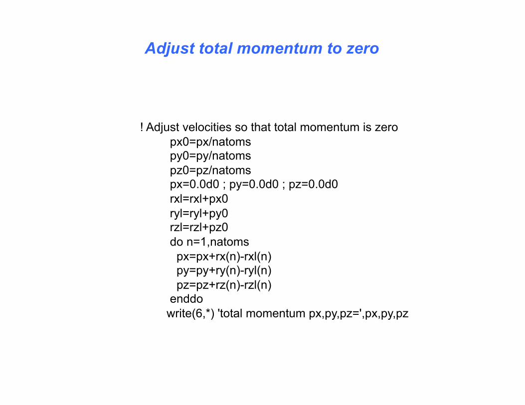
Adjust total momentum to zero

! Adjust velocities so that total momentum is zero px0=px/natoms py0=py/natoms pz0=pz/natoms px=0.0d0 ; py=0.0d0 ; pz=0.0d0 rxl=rxl+px0 ryl=ryl+py0 rzl=rzl+pz0 do n=1,natoms px=px+rx(n)-rxl(n) py=py+ry(n)-ryl(n) pz=pz+rz(n)-rzl(n) enddo write(6,*) 'total momentum px,py,pz=',px,py,pz

Beginning of MD loop

! Integrate MD do n=1,nstep fx=0.0d0 ! Zero initial x-component of forces fy=0.0d0 ! Zero initial y-component of forces fz=0.0d0 ! Zero initial z-component of forces epot=0.0d0 ! Zero the total potential energy ekin=0.0d0 ! Zero the total kinetic energy

Loop on pairs, forces, energy calcultion… do i=1,natoms-1 do j=i+1,natoms rxij=rx(i)-rx(j) ryij=ry(i)-ry(j) rzij=rz(i)-rz(j) sxij=rxij/h1 syij=ryij/h2 szij=rzij/h3 sxij=sxij-dble(anint(sxij)) syij=syij-dble(anint(syij)) szij=szij-dble(anint(szij)) rxij=sxij*h1; ryij=syij*h2; rzij=szij*h3 rij=dsqrt(rxij**2+ryij**2+rzij**2) if(rij.lt.rcut) then sovr=sigma/rij epot=epot+4.0d0*epsilon*(sovr**12-sovr**6)-vcut+fcut*(rij-rcut) fij=(24.0d0*epsilon/rij)*(2.0d0*sovr**12-sovr**6)-fcut fx(i)=fx(i)+fij*rxij/rij fy(i)=fy(i)+fij*ryij/rij fz(i)=fz(i)+fij*rzij/rij fx(j)=fx(j)-fij*rxij/rij fy(j)=fy(j)-fij*ryij/rij fz(j)=fz(j)-fij*rzij/rij endif enddo enddo

Advance atoms and compute kinetic energy

! Verlet algorithm to move atoms, compute kinetic energy do i=1,natoms rxx=2.0d0*rx(i)-rxl(i)+fx(i)*dt**2/(amass) ryy=2.0d0*ry(i)-ryl(i)+fy(i)*dt**2/(amass) rzz=2.0d0*rz(i)-rzl(i)+fz(i)*dt**2/(amass) vx=(rxx-rxl(i))/(2.0d0*dt) vy=(ryy-ryl(i))/(2.0d0*dt) vz=(rzz-rzl(i))/(2.0d0*dt) vsq=vx**2+vy**2+vz**2 ekin=ekin+0.5d0*amass*vsq rxl(i)=rx(i) ryl(i)=ry(i) rzl(i)=rz(i) rx(i)=rxx ry(i)=ryy rz(i)=rzz enddo

Last bit of MD loop, compute and output energy

! Output kinetic, potential, and total energy per atom time=time+tunit*dt if(mod(n,iavpro).eq.0) then ekin=ekin/natoms; epot= epot/natoms; etot=epot+ekin temp=(2.0d0/3.0d0)*eps*ekin ! Temperature ekin=ekin*(8.617d-5)*eps ! Kinetic energy in eV epot=epot*(8.617d-5)*eps ! Potential energy in eV etot=etot*(8.617d-5)*eps ! Total energy in eV write(6,100) n,time,ekin,epot,etot,temp ! Time in picoseconds endif enddo 100  format(i8,f12.2,4f18.6)

Radial distribution function do i=1,natoms-1 do j=i+1,natoms rxij=rx(i)-rx(j) ryij=ry(i)-ry(j) rzij=rz(i)-rz(j) sxij=rxij/h1 syij=ryij/h2 szij=rzij/h3 sxij=sxij-dble(anint(sxij)) syij=syij-dble(anint(syij)) szij=szij-dble(anint(szij)) rxij=sxij*h1; ryij=syij*h2; rzij=szij*h3 rij=dsqrt(rxij**2+ryij**2+rzij**2) if(rij.le.rcut) then nb=int(rij/delr) g(nb)=g(nb)+2.0d0 endif enddo enddo do nb=1,nbins rij=delr*nb fac=3.0d0*volume/(4.0d0*pi*natoms**2) fac=fac/((rij+delr)**3-rij**3) g(nb)=fac*g(nb) write(6,*) rij,g(nb) enddo