Embed Size (px)
Citation preview

Arch. Hist. Exact Sci. 55 (2001) 395–422.c© Springer-Verlag 2001
History and Epistemology of Models:Meteorology (1946–1963) as a Case Study
Amy Dahan Dalmedico
Communicated byI. Schneider
Abstract
This paper focuses on scientific practices and problems of modeling in the case ofmeteorology. This domain is especially interesting because of its crucial influence onthe conception of mathematical models and its links with numerical instability, comput-ers, and the science of chaos and dynamic systems. All of these questions involve fortheir solution a considerable mathematical apparatus which was developed by severalmathematicians.
An early example is von Neumann’s and Charney’s Princeton Meteorological Pro-ject in the period 1946–53 which ended with daily numerical prediction in less than 2hours. After this stage, the questions of long-range forecasting and general circulation ofthe atmosphere became of greater importance. The late 1950s saw the emergence of analternative: were atmospheric models used mainly for prediction or understanding? Thiscontroversial debate in particular occurred during an important colloquium in Tokyoin 1960 which gathered together J. Charney, E. Lorenz, A. Eliassen, and B. Saltzman,among others, and witnessed discussions on statistical methods for predictions and/ormaximum simplification of dynamic equations. This phase ended in 1963 with Lorenz’sseminal paper on “Deterministic non periodic flows.”
Introduction
In the history of the relationship between mathematics and the natural world, onemay discern a transition from an era of applied mathematics best associated with the ex-pression “mathematization” (of physical phenomena) to a new era in scientific practicewhich, albeit appearing in the 1930s, was mainly developed after the Second World Warand which is associated with expressions such as “modeling.” In the aftermath of thewar, important transformations occurred in both the social and the technological realmsthat fostered the development of a mathematical understanding of the world. On the onehand, as John von Neumann’s career aptly symbolizes, the status of the mathematicianchanged significantly.1 The image of the mathematician more or less locked into his
1 These questions will not be developed here. See Dahan Dalmedico [1996].

396 A. Dahan Dalmedico
academic milieu was replaced by that of an expert close to the political power and whowas the ‘manager’ of big scientific and technological projects. On the other hand, withthe development of increasingly powerful computational technologies, new possibilitiesand challenges arose which gave rise to innovative modeling practices. Epistemologicaltensions between statistical and deterministic models were made manifest by these newpractices. In particular, the alternative between understanding and operating or predict-ing became one of the most important aspects of science in the second half of the century,in physics (as discussed by Paul Forman in the case of quantum electrodynamics), butalso in applied mathematics.
I have selected the case of meteorology for the present study because, in my opin-ion, it is particularly emblematic of the shift from mathematization to modeling. Setup in part by von Neumann immediately after the end of World War II, the PrincetonMeteorological Project was explicitly intended as a means of transforming the socialsettings in which research was conducted from an individual to an essentially collectiveendeavor. Moreover, meteorology was among the first scientific disciplines where theadvent of numerical methods transformed the mathematical practice of its scientists.As William Aspray wrote in his biography of von Neumann, the “computer almosttransformed meteorology into a mathematical science.”2 Therefore, meteorology madethe tensions, between statistics and dynamics, between prediction and understanding,especially acute. One may even argue that it was in the conflict between predicting(and indeed controlling) the weather and understanding the atmospheric system thatthese epistemological tensions initially surfaced most forcefully. This crucial role ofcomputers and numerical simulations merits further examination.
I will first briefly sketch what meteorology and meteorological practices were likeduring the early 20th century, before the computer era. Then, I deal with the beginningsof von Neumann’s Electronic Project and his Meteorological Numerical Project. In thesehistorical accounts, I rely mainly on W. Aspray’s and F. Nebecker’s books.3 However, Ifocus on the epistemological aspects of modeling practices in order to better illuminatethe drastic changes which occured in the late 1950’s and which I discuss in the remainderof the article.
I. Meteorology before the computer era
Up until the middle of the 20th century scientific interest in the weather involvedthree kinds of activity:
1) An empirical activity consisting of recording observations, and then trying to infersomething from the recorded data. Generally, thisempirical traditionwas mainlyinterested in the production of an “average weather” and was characterized as adescriptive science – called ‘climatology’ – mainly based on weather statistics.
2) A theoretical activity striving to explain atmospheric phenomena on the basis ofgeneral principles. Using the laws of physics as its starting point, thistheoretical
2 Aspray [1990], p. 152.3 Aspray [1990], Nebeker [1995].

Models in Meteorology (1946–1963) 397
tradition established dynamical meteorology as a scientific discipline. In compos-ing their treatises, however, theorists seldom used the large amount of availablemeteorological data.
3) A practical activity concerned with weather prediction. Forecasters based their pre-dictions on only a small amount of data and hardly any theory at all. Hence theirwork was regarded by the two other groups as unscientific. More an art than ascience, forecasts were founded on individual experiences, a few elementary sta-tistical relations, and some qualitative physical arguments, rather than on theory orthe application of general methods and procedures. Thesynoptic tradition, as it wascalled, studied some characteristic structures by means of which the atmospherecould be analyzed. Thanks to their “know-how”, synopticians were supposedly ableto recognize how these structures changed and to detect signals announcing theirappearance or disappearance.
Connections among these three separate traditions became stronger and more nu-merous in the first half of the 20th century. Transformations occurred, which later led totheir unification. But, although several attempts were made to introduce objective meth-ods based on theoretical foundations, until 1950 no one was able to match the successof the earlier subjective methods of forecasting. No significant increase in the accuracyof short-range predictions resulted. Unification hinged mainly on the new availability offast computing machines.
Two men are particularly important during this first period: Vilhelm Bjerknes andLewis Fry Richardson. In 1903 Bjerknes, a Norwegian physicist who had turned to me-teorology, became an advocate for the computational approach to weather forecasting.He wished to bring the full range of observations together with theory in order to predictthe weather. He was the first to identify key-concepts such asbaroclinicity andbaro-tropicity.4 In his 1904 program, Bjerknes wrote: “We forgo any thought of analyticalmethods of integration and instead, pose the problem of weather prediction in the follow-ing practical form:Based upon the observations that have been made, the initial state ofthe atmosphere is represented by a number of charts which give the distribution of sevenvariables from level to level in the atmosphere. With these charts as the starting point,new charts of a similar kind are to be drawn which represent the new state from hourto hour.” 5 However, no analytic methods for solving the physical equations involved inthis procedure were known at that time, and so Bjerknes was forced to rely mainly ongraphical methods.
Richardson’s 1922 program
The next person to try to carry out Bjerknes’s program was the English scientistLewis Fry Richardson. Perhaps, as Aspray suggested, it was the hope of applying a
4 A model isbarotropicwhen pressure depends on the location only, not on the local height;it is baroclinic when a vertical pressure component is incorporated which takes into account themixing of the air and the loss of potential energy.
5 Aspray [1990], p. 126.

398 A. Dahan Dalmedico
numerical method for solving partial differential equations (which he had discoveredwhile working in industry) that led Richardson to turn towards meteorology. Shortlyafter World War I, he devised an algorithmic scheme for weather prediction based onthis method. In 1922, Richardson published his bookWeather Prediction by NumericalProcess, which became well known. It opened with an analogy between astronomy andmeteorology, leading up to the following critical remark: “The forecast is based on thesupposition that what the atmosphere did then [at a previous time when the weather con-ditions were similar], it will do again now....The past history of the atmosphere is used,so to speak, as a full-scale model of its present self.” Richardson went on: “But – onemay reflect – theNautical Almanac, that marvel of accurate forecasting is not based onthe principle that astronomical history repeats itself in the aggregate. It would be safe tosay that a particular disposition of stars, planets, and satellites never occurs twice. Whythen should we expect a present weather map to be exactly represented in a catalogueof past weather?”.6 Here Richardson implicitly referred to the dominant synoptic pointof view of which he strongly disapproved. Following Bjerknes’s program, he advocatedthe use of differential equations and analytic methods.
Richardson set out to formulate seven equations that would completely determinethe behavior of the atmosphere given its initial state. The first three equations are essen-tially Newton’s law (force equals mass times acceleration). The fourth equation says thatif the mass-density decreases at a place, than matter must have moved away. The fifthsays the same for the water content. The sixth says that an addition of heat must eitherraise the temperature or do work or both. There is also a seventh equation (not writtenhere) which is a combination of Boyle’s law (that pressure is inversely proportional tovolume) and Charles’ law (that volume is directly proportional to absolute temperature)with an allowance made for the presence of water vapor.
In the following, we summarily describe Richardson’s procedure, which becamecanonical much later.7
The six equations are:∂u
∂t= −u∂u
∂x− v
∂u
∂y− w
∂u
∂z− f u− 1
p
∂p
∂x
∂v
∂t= −u∂v
∂x− v
∂v
∂y− w
∂v
∂z− f u− 1
p
∂p
∂y
∂w
∂t= −u∂w
∂x− v
∂w
∂y− w
∂w
∂z− g − 1
p
∂p
∂z
∂ρ
∂t= −u∂ρ
∂x− v
∂ρ
∂y− w
∂ρ
∂z−
(∂u
∂x+ ∂v
∂y+ ∂w
∂z
)
∂p
∂t= −u∂p
∂x− v
∂p
∂y− w
∂p
∂z− Cp
Cvp
(∂u
∂x+ ∂v
∂y+ ∂w
∂z
)
6 Ibidem, p. 127. Emphasis mine.7 Ibidem, pp. 124–127. See also Nebecker [1995], pp. 65–67.

Models in Meteorology (1946–1963) 399
∂T
∂t= −u∂T
∂x− v
∂T
∂y− w
∂T
∂z− RT
Cv
(∂u
∂x+ ∂v
∂y+ ∂w
∂z
)
whereu, v,w, are components of the fluid velocity in thex, y, z directions;Cp repre-sents the heat coefficient at constant pressure,ρ the local mass density of the fluid,fthe Coriolis parameter,p the ambient pressure,g the constant of gravity, and, finally,Cvthe specific heat at constant volume.T is the absolute temperature,R is the gas constantrelated to Avogadro’s number.
These equations imply that the time derivatives can be expressed in terms of spatialderivatives.
– Observational data for all independent variables in the equations are collected at aninitial time t at each point of a finite grid evenly distributed over a region of theatmosphere.
– The method of finite differences is used as an approximation of spatial derivatives,and the time derivatives are then computed by means of the equations above.
– In this way, the values of the parameters at each point of the grid are extrapolated toa time shortly thereafter,t +�t .
– Using the extrapolated data, this procedure is then repeated and values att +2�t areevaluated. This process is repeated again and again, as many times as necessary toextend the prediction to a desired time interval.
Unfortunately, for a “forecast” extending over a 6-hour period, Richardson neededsix weeks of intensive labor in order to complete the computations! Needless to say, thiswas discouraging. Richardson imputed the impracticability of his method mainly to thedramatic slowness of the computation.
Numerical instability
Before World War II, only one relevant important advance took place concerningthe numerical methods for solving partial differential equations. It was presented ina paper written in 1928 in Gottingen by Richard Courant and his two young as-sistants Karl Friedrichs and Hans Lewy.8 Their initial idea was to use a method ofnumerical approximation (the method of finite differences) in order to demonstratethe existence of solutions of partial differential equations. Elaborating this idea, theydiscovered a new phenomenon – callednumerical instability– which would laterturn out to be exceptionally important in the development of numerical methods.When one replaces a differential equation by a set of numerical equations howeverclose to the given equation, solutions of these approximating equations may havenothing to do with the solutions of the original equation.9 The three mathematiciansshowed that the solutions of the finite-difference equations converged towards thesolution of the differential equation only if the grid of the finite-difference equations
8 Courant, R., Friedrichs, & Lewy, [1928].9 Goldstine [1972], p. 288.

400 A. Dahan Dalmedico
satisfied the following condition (later to be called the ‘Courant condition’): the ratio�t/�x of the time step to the space step is less than a numberC depending onlyon the differential equation and the initial conditions. If on the contrary the Courantcondition was not met, they showed, errors would increase without limit. The papercontained a rigorous criterion for stability in the cases of hyperbolic and parabolicequations with constant coefficients in one dependent, or two independent, vari-ables. Later, von Neumann generalized this last condition in a heuristic, rather thanrigorous, fashion, and although he lectured on it several times he never publishedthe result.10
World War II: a “near discontinuous change” in meteorological practice
During the Second World War, forecasts were vital military information and crit-ical for the planning of military operations. The secrecy and reliability of weatherpredictions could have strategic importance, such as, for example, the choice of theday for Operation Overlord. World War II created a huge demand for meteorolo-gy and hence for meteorologists. Major changes that occurred during the war in-cluded:11
– New subjects and interests emerged; when planes flew at much greater heights, fore-casters were asked about clouds, ice formation, fog and high-level winds. As a resultof the new abundance of upper-air data, physics became more relevant to forecasters’work. However, attempts to increase the range of the forecasts to more than two orthree days were recognized as hardly realistic.
– About six or seven thousand meteorologists were trained in various laboratoriesduring the war. The total strength of the Air Weather Service reached 19,000while the Navy’s Aerological Service employed 6,000 more. An urgent need totrain a large number of people very rapidly may have indirectly contributed tomaking meteorology more mathematical, more formalized, and also more theo-retical.
– Observational methods and weather data records were standardized.– The use of punched-card machines, and the automation of data-processing in mete-
orology increased dramatically.– The meteorological forecasting practice became a group activity focusing on specific
tasks.– Important research topics changed, and objective forecasting was favored over the
synopticians’ subjective methods.
10 Lectures of von Neumann at Los Alamos Laboratories in February 1947 and letters fromvon Neumann to the mathematician Werner Leuter (October, 15, 1950, and November, 10, 1950)mentioned by Aspray [1990], p. 286 f. notes 27 and 28. See also von Neumann & Richtmyer[1950], and Goldstine [1972].
11 Nebeker [1995], pp. 111–132; Saltzman [1967]; Thompson [1983].

Models in Meteorology (1946–1963) 401
Von Neumann’s electronic and meteorology projects
In the 1940s, the mathematician John von Neumann initiated a significant rear-rangement of interests concerning hydrodynamics, computers, and numerical analysis.Because of his work at Los Alamos on nuclear reactions, he was convinced that hydro-dynamics was of crucial importance to physics and mathematics, and he was one of thefirst to realize that it required radically new developments in computational resources.In 1945, in a memorandum sent to O.Veblen, von Neumann wrote:
A further experience which has been acquired during this period [World War II] is thatmany problems which do not prima facie appear to be hydrodynamical necessitate thesolution of hydrodynamical questions or lead to calculations of the hydrodynamical type.It should be noted that it is only natural that this should be so since hydrodynamical prob-lems are the prototype for anything involving non-linear partial differential equations,particularly those of the hyperbolic or mixed type, hydrodynamics being a major physi-cal guide in this important field, which is clearly too difficult at present from the purelymathematical point of view.12
Hydrodynamics appeared to von Neumann as the prototype for non-linearity. Whileelectronic computers existed merely in his imagination, he insightfully declared in 1945:“Many branches of pure and applied mathematics are in a great need of computing in-struments to break the present stalemate created by the failure of the purely analyticalapproach to non-linear problems.”13 In 1946, a program for the building of an electroniccomputer – the Electronic Computer Project – was launched at the Institute for AdvancedStudy at Princeton under his direction.14 As a large-scale application of the Electron-ic Project, von Neumann chose numerical meteorology, which he judged strategic. Hesucceeded in convincing the Navy to support the project.
On August 29 and 30, 1946, von Neumann organized a conference in Princeton inorder to acquaint the meteorological community with the electronic computer being builtat the Institute and to solicit their advice and support in designing research strategies. Aconsensus emerged that six areas merited study, the three most interesting of which were:numerical methods for solving important differential equations by means of the com-puter, tropical hurricane theory, and forecasting by direct numerical methods.15 Duringthe first two years of the Meteorology Group set up after von Neumann’s conference, aseries of exploratory investigations was conducted. The main one concerned the systemof hydrodynamic equations of atmospheric flow and, because it became apparent thatthe basic equations were ill-suited to numerical as well as analytical solutions, theirsystematic simplification for direct integration was undertaken.
Albert Cahn and Philip Thompson simplified the mathematical model of atmosphericflow so that it retained important meteorological phenomena whilefiltering outnon-me-teorological ones, such as gravity and sound waves. Thisfiltering processhad alreadybeen implicitly practiced by meteorologists when formulating their theories. In the first
12 Memorandum, 26th March 1945. Von Neumann, Works VI, pp. 357–359.13 Works, V, p. 2.14 See Aspray [1990], pp. 49–94 and Goldstine [1972], pp. 208–234.15 Aspray [1990], p. 17.

402 A. Dahan Dalmedico
two years of the project, Paul Queney and Thompson introducedfiltered modelswhichthey checked against meteorological data.16 But, as Aspray has noticed, “Jules Charneywas the first to make this procedure explicit and recommend it as the most promisingapproach for numerical meteorology”.17 In 1947, Charney used a metaphor which wasto become famous: “This leads us to the next problem, namely, how to filter out thenoise. Pardon me, but let us again think metaphorically.The atmosphere is a transmitter.The computing machine is the receiver. . . . Nowthere are two ways to eliminate noisein the output. The first is to make sure that the input is free from objectionable noises,or the second is to employ a filtering system in the receiver.”18 In fact, when Charneytook the lead of the Meteorological Project, this metaphor expressed the basic idea ofhis methodology of atmospheric modeling.
II. Von Neumann’s and Charney’s program (1946–53)
With Jules Charney’s arrival in the summer of 1948, the Meteorological Project tooka new direction: the work of the group became much more unified, goal-oriented, andwas summarized in two annual reports. Under Charney’s directorship, resources andearlier, parallel investigations were focused through a single approach: “to consid-er a hierarchy of ‘pilot problems’ embodying successively more and more of thephysical, numerical, and observational aspects of the general forecast problem.” Theobjective of the project was clear: “the development of a method for the numericalintegration of the meteorological equations which is suitable for use in conjunctionwith the electronic computing machine now under construction at the Institute forAdvanced Study.”19
The methodology of “theory pull”
Charney and his colleagues adopted a progressive process through which algo-rithms could be implemented with small incremental steps. The algorithms consid-
16 The basic equations such as the set of equations Richardson used can be said to describetoo much since they admit solutions that correspond to types of motion that are not meteorologi-cally significant, especially higher-frequency wave motions such as sound waves, gravity waves,slow inertial waves etc. The Report of Progress of the Meteorology Project for the year 1947concluded: “. . . it might simplify matters considerably if those equations were somehow informedthat we are interested in certain kind of atmospheric behavior – i.e, the propagation of large-scaledisturbances. This is tantamount to constructing a ‘mathematical filter’ to remove ‘noise’ andotherwise unwanted regions of the spectrum.” The process of filtering consists in separating themeteorologically significant solutions from the insignificant ones.
17 Aspray [1990], p. 139.18 Letter to P. Thompson, February, 12, 1947, quoted by Aspray [1990], p. 300, note 73;
emphasis is mine.19 Progress Report of the Meteorology Group at the Institute of Advanced Study, July 1,
1948 to June 30, 1949, JCMI. quoted by Aspray [1990], p. 139.

Models in Meteorology (1946–1963) 403
ered also depended on computer feasibility, which itself was continuously evolving.One started from a simplified model whose behavior could be computed; one com-pared how the predictions of this model fitted observed phenomena; then one alteredthe model, generally by adding a physical factor whose previous exclusion, the sci-entists thought, was the cause of important observed distortions. Charney called thisapproach “theory pull”.
In 1949, Charney suggested a “two-dimensional barotropic” model20 as the group’sobject of study and he studied numerical properties of linearized barotropic equations inorder to anticipate the numerical integration of nonlinear equations. Charney was awarethat Richardson’s algorithm does not satisfy Courant’s condition so that its repeated ap-plication was computationally unstable and could not give useful results. But he foundthat by filtering out most atmospheric motions he made it much easier to satisfy theCourant condition, which in this case becomes: the time increment must be less than thetime required for a wave impulse to be transmitted from one grid point to another. Basedon the principle of conservation of vorticity, Charney’s model retained only observedvariables while filtering out waves traveling faster than what was allowed by Courant’scondition (sound and gravity waves in particular). Thompson later explained:
Charney’s 1947 formulation, later known as the quasi-geostrophic model [motion is saidto be quasi-geostrophic when there is an approximate balance between the pressure-gra-dient force and the Coriolis force],simultaneously skirted two major difficulties: first, itimposed much less stringent conditions for computational stability, and second, it did notdemand that the horizontal divergence or accelerations be computed as small differencesbetween large and compensating terms, each of which is subject to sizable percentage er-rors. These features alone evaded the two fundamental difficulties inherent in the practicalapplication of Richardson’s method.21
The integration was done on the ENIAC computer, and numerical stability was stud-ied according to the methods introduced in Courant, Friedrichs, and Lewy’s paper.
In 1950, Charney, Ragnar Fjotoft, and von Neumann published their first report,which contained an analysis of the equations they used and a summary of predictionsover a period of 24 hours, for four chosen days in 1940. Earlier ENIAC computationsand other studies indicated that the atmosphere behaved barotropically over long timeperiods. The above model therefore performed satisfactorily during these periods. Basedon vorticity conservation, however, it was unable to take into account the formation, in-tensification, or dissipation of storms. Further attempts were made to improve the modelin this direction.
20 As explained in note 4, a model isbarotropic when pressure is considered constant andbaroclinic when a vertical component is incorporated which takes into account its variation. Inhis 1949 model, Charney assumed (1) a uniform density for the atmosphere, (2) purely horizontalmotion, (3) the coincidence of constant density and constant pressure surfaces (barotropy), (4) anapproximate balance of the pressure gradients produced and the Coriolis force (quasi-geostrophy),(5) the constancy over time of the vorticity of a fluid element around its vertical axis (vorticityconservation), (6) parallel streams of wind at all levels, and (7) the thermodynamic closure of thesystem. See Aspray [1990], p. 301.
21 Thompson [1983], p. 760.

404 A. Dahan Dalmedico
In 1951, another meteorologist on the team, Norman Phillips, introduced abaroclinicmodel, formed by two barotropic, incompressible, and homogeneous levels of differentdensities, which provided almost the same features as a fully three-dimensional model.Although the model predicted cloudiness and precipitation with reasonable accuracy, theimprovements were not judged satisfactory by von Neumann and Charney, because thistwo-layer model had not predicted the rapid development of the Thanksgiving weekendstorm. Charney then used athree-level modelwhich correlated better with predictions. In1953, additional baroclinic forecasts were made with three-, five- and even seven-layer,models to try to take into account certain kinetic and dynamical effects such as, amongothers, the horizontal-vertical vorticity conversion.
On August 5, 1952, von Neumann called a meeting at Princeton, which gatheredmembers of the Weather Bureau, the Navy, and the Air Force. His goal was to assessthe operational value of numerical meteorological prediction. In order to reach 24-hourforecasts over the whole territory of the United States, he advocated the use of a generalbaroclinic model which he thought could be valid over periods up to 36 hours. He arguedthat altogether the total time required for collecting and preparing data, and computing,treating, and printing results should not exceed 12 hours. Less than one year later this aimwas achieved. The group’s report stipulated that “the trend in the application to short-range prediction of the quasi-geostrophic model equations had become so predictablethat this phase of the work had ceased to be – for the Project – a matter of major scientificinterest.”22 Henceforth, kept busy by his other responsibilities (in particular as a memberof the Atomic Energy Commission), John von Neumann no longer participated in theMeteorology Group.
The computer: an inductive machine for physical models in meteorology?
After his first important successes, Charney wrote in 1952 that: “The philosophyguiding the approach to this problem [of numerical prediction] has been to constructa hierarchy of atmospheric models of increasing complexity, the features of each suc-cessive model being determined by an analysis of the shortcomings of the previousmodel.”23
The “theory pull” methodology led to a series of “physical models” of the atmosphere,in the sense that they were based on simplifiedphysicalhypotheses and yet they weremeant to copy the atmospheric behavior. Thompson’s early filtered models, Charney’stwo-dimensional barotropic model, Phillips’ baroclinic model, Charney’s three-levelmodel, additional baroclinic models etc, belonged to this type of physical models; theywere mainly developed for predicting the weather. In the first stage of the computer era,the trend had been to adjust oversimplified physical models of atmospheric behaviorby making them more complicated. As agiant calculator, the computer made possiblethe treatment of increasingly involved equations that provided better descriptions of the
22 Meteorology Project, Quaterly Progress Report, July 1, 1953 to March 31, 1954 (Jule Char-ney Papers, MIT Archives).
23 Meteorology Project Reportquoted in Aspray [1990], p. 302.

Models in Meteorology (1946–1963) 405
atmosphere and therefore gave hope for more precise predictions. But meteorology wasalso highly constrained – and this is still the case – by electronic computers. Their perfor-mance capacity, the size of their memories, the restrictions on arithmetic operations, theselection of numerical methods convenient for electronic computations, and their limit-ed dependability constituted unavoidable factors that transformed meteorology into anengineering science.24
In a lecture addressed to the National Academy of Sciences in 1955, Charney ana-lyzed the role played by the computer in his discipline:
The advent of the large-scale electronic computer has given a profound stimulus to thescience of meteorology. For the first time, the meteorologist possesses a mathematical ap-paratus capable of dealing with the large number of parameters required for determiningthe state of the atmosphere and of solving the nonlinear equations governing its motion.Earlier, for want of such an apparatus, both the forecaster and the investigator were forcedto content themselves with such highly oversimplified descriptions or models of the at-mosphere that forecasting remained largely a matter of extrapolation and memory, anddynamical meteorology a field in which belief in a theory was often more a matter of faiththan of experience. Needless to say, the practicing meteorologist could ignore the resultsof theory with good conscience.25
Charney went even further. He envisioned new and promising roles for the com-puter:
The radical alteration that is taking place in this state of affairs is due not merely to theability of the machine to solve known equations with known initial and boundary con-ditions but even more to its ability to serve as an inductive device. The laws of motionof the atmosphere, especially as they concern the dynamics of the largest motions andtheir energy-exchange processes, are very imperfectly known. The machine, by reducingthe mathematical difficulties involved in carrying a physical argument to its logical con-clusion, makes possible the making and testing of physical hypotheses in a field wherecontrolled experiment is still visionary and model experiment difficult, and so permits awider use of inductive methods.26
Therefore, Charney suggested that the computer could be used as aninductive ma-chinewhich could test selected physical hypotheses. A few years later, this same ideawould lead to a very different kind of model in meteorology: the so-called “laboratorymodels”. These differed from the physical models in that they didn’t copy atmosphericbehavior in order to predict but instead generated theoretical situations in order to un-derstand specific atmospheric phenomena. We will study this point in the third part ofthis paper.
E.N. Lorenz reconstructed, in 1960, the entire procedure used for obtaining theequations of numerical weather prediction from the fundamental laws governing theatmosphere. He looked at the system of these equations from both a physical point ofview (gauging the significance of different physical hypotheses and that of their simpli-
24 See Phillips [1960].25 Charney, J. [1955] in Aspray [1990], p. 152.26 Charney, J.,Ibidem, p. 153.

406 A. Dahan Dalmedico
fication) and from a mathematical point of view (studying the dependency of variables,the separation of the equations in different groups, the role of differential operators, etc).He distinguished the following steps:27
– For a dry atmosphere, the physical laws determine the well-known set of six equations(Richardson’s equations cited above).
– The equation of vertical motion – the third equation of Richardson’s system – isfirst discarded, and replaced by the so-called “hydrostatic equation”. Slightly mod-ified with the help of the time derivative of the hydrostatic equation, this system isgenerally called theprimitive equation.
– The new system is then expressed in terms of two independent variables: pressureand height. Horizontal wind components are expressed in terms of vorticity and di-vergence (a differential operator applied to the movement).
– This last equation is then discarded and replaced by theequation of balanceobtainedby dropping out all terms containing a divergence from the previous equation. More-over, it is often more convenient to omit certain additional terms from the equationof balance, reducing it to thegeostrophic equation.
– The equation of balance and the geostrophic equation are often calledfiltering ap-proximations, since they eliminate the occurrence of certain waves that can occur insystems governed by the primitive equations, but are often considered irrelevant.
– Finally the vertical dimensions can be replaced by a small number of layers. Eachfunction depending on time and on the three spatial dimensions is then replaced byseveral functions of time and two spatial dimensions.
It is important to emphasize that Lorenz’logical reconstructionhas nothing to dowith the historical developmentof the simplified equations (for example, the filteredequations appear here as a last step, whereas, historically, filtering was the first issueaddressed). The historical development was determined by interactions among numer-ical results, observed and measured physical results, the availability of computationalmachines, and the availability and rapidity of computing methods. In fact, then, thedevelopment of the practice of modeling followed a very different route than might beassumed on the basis of logic.
III. The debate about models (from the late 1950s to 1963)
In the late 1950s, it became obvious that the so-called “filtered equations”,28 whichmade numerical weather predictions possible with the first computers, would no longerbe able to provide predictions of as high a quality as was now required for long-rangeforecasting. Consequently, the general attitude was either to return to the primitive hydro-dynamic equations, given the advent of more powerful computers, or to extend filtering
27 E.N. Lorenz [1960a], p. 366. We summarize the big lines of this reconstruction to give anidea of the relationships between the different systems of equations (without entering into details)and to introduce their names.
28 As we already explained, the filtering process had been practiced by meteorologists for a longtime; after 1947 and Charney’s metaphor, the expression ‘filtered equations’ became canonical.

Models in Meteorology (1946–1963) 407
principles; this second way led to so-called balance equations.29 Both ways concernedwhat we have called above “physical models” of the atmosphere. But another attitudebegan to emerge, which raised the very question of predictability and introduced the useof “laboratory models.” This last expression will be elucidated below.
Statistics and predictability
In the 1950s, statistical methods prevailed in many areas of science. In particularthey were seen as appropriate tools for understanding disorderly phenomena. Althoughsome well-known results of Henri Poincare and George D. Birkhoff proved that the op-position between order and disorder was not so radical as had been thought,30 statisticalmethods appeared to be the only adequate ones for studying such phenomena. This wasthe case not only in physics, mechanics (with the ergodicity concept), fluid mechanics(with Kolmogorov’s statistical theory of turbulence elaborated in 1941), astrophysics(where Neymann, Scott, and Shana31 studied the distribution of galaxies by statisticalmethods), dynamics of epidemics (Bartlett’s work32), but also in biology and populationgenetics. A series of annual symposia at Berkeley on mathematical statistics provides agood picture of the spectrum of research from very different fields in which mathematicalstatistics was the primary method of investigation.
In meteorology, two trends in fact coexisted: the first privileged statistical meth-ods, the second, deterministic dynamics. Meteorologists debated the attendant merits ofboth. Von Neumann’s initial approach had been to use fast computers to solve dynami-cal equations of atmospheric movement. The race of the computer against time that helaunched – to provide predictions of the weather 24 hours in advance in less than 24hours – had succeeded. It seemed his optimism for accurate predictive analysis had paidoff. In a certain sense, even if he was absolutely convinced that long-term forecastingwas a meteorological illusion, his goal remained the mastery and control of instabilities,approximations, and errors in initial data and observations. These could – and should –be overcome by computing methods. Furthermore, von Neumann held on to the dreamaccording to which the knowledge of the effects of a disturbance on general meteoro-logical features would enable humankind tocontrol the weather. Norbert Wiener, on theother hand, was critical of this approach. He was much more sensitive to randomnessand believed it to be fundamentally impossible to gain this kind of weather control.Instead, he stressed that models needed to take into account from the outset the fact thatinformation and knowledge would be always incomplete. Wiener had always been very
29 This is explained in J.G. Charney [1962].30 Let us mention the difficulties raised by the interpretation of the Fermi-Pasta-Ulam numer-
ical experiment. Ergodicity allowed the use of statistical methods, but the mixing between orderand disorder revealed by this experiment resisted any mathematical formulation. At the Interna-tional Congress of Mathematicians of Amsterdam in 1954, Kolmogorov’s announcement of hisresult on dynamical systems – later known as the Kolmogorov-Arnold-Moser (KAM) theorem –would drastically change the picture. Fermi, Pasta & Ulam [1947] in Ulam [1974].
31 Proceedings[1955], vol III, p. 75.32 Idem, vol IV, p. 81.

408 A. Dahan Dalmedico
fond of formulating scientific problems in terms of time-varying statistical processes. Hegave a mathematical theory of the Brownian motion, considered as a special prototypeof these processes. He strongly advocated the use of statistical methods for all problemsof prediction33; for meteorology, that meant formulating the problem of prediction interms of statistical properties of past weather and not in terms of deterministic dynamics.
At the third Berkeley Symposium on mathematical statistics, Wiener cited Shake-speare in support of sensitivity to initial conditions:
for want a nail, the shoe was lost.for want a shoe, the horse was lost.for want a horse, the rider was lost.for want a rider, the battle was lost.for want a battle, the kingdom was lost.34
Wiener suggested leaving exact computations to the exact sciences and adoptingstatistical methods in all other areas of science. He underlined “the very real possibilityof the self amplification of small details in the weather map,” but he did not know the or-igin of these instabilities nor their actual frequency any better than von Neumann. Whatopposed the two mathematicians, as Steve Heims has pointed out, was more a questionof conviction, of metaphysics, or, let us say, of conception of world (Weltanschaung).35
In particular, time and error play a different role in their respective works.Like the majority of meteorologists, Edward Lorenz had for several years used
statistical methods as he was involved in an experiment performed by the StatisticalForecasting Project at MIT. Lorenz thought that in meteorology: “philosophically, sta-tistical prevision is more like synoptic meteorology than dynamical prediction, becauseit is founded more on observations of what happened in the past than on physical prin-ciples.” The most common method in statistical forecasting, linear regression, requiredvery long mathematical procedures in order to estimate the best values for its constants.But linear regression methods often failed to yield good weather forecasts; this hap-penned either because the weather was basically unpredictable from currently availableinitial data, or because linear methods were inadequate. During the MIT experiment,meteorologists generated a series of “weather maps” through the numerical integrationof a set of nonlinear differential equations (i.e. by dynamical prediction), then, they at-tempted toreproducethese maps by means of linear regressions. On this basis, in 1960,Lorenz had reached the conviction that the statistical method was invalid. He presentedhis results during a Symposium held in Tokyo, which became a turning point for thecommunity, and is particularly instructive for us36.
Those who favored linear regression methods could draw on a theorem of Wiener’sshowing that if a statistically stationary system was ‘deterministic’, in the sense that itcould be predicted exactly from the knowledge of its own present and past by some for-
33 During World War II, Wiener worked also on a statistical theory of prediction; he presentedit at the International Congress of Mathematicians in 1950 at Harvard.
34 Wiener [1956], p. 248.35 see Heims, [1980] pp. 116–162.36 Lorenz [1960b].

Models in Meteorology (1946–1963) 409
mula, then it could also be predicted exactly from its own present and past by somelinearformula. The linear formula might involve an infinite quantity of past data and manyterms might be required for a good approximation. From the meteorologists’ standpoint,the important question was whether there was a nearly perfect linear formula involvingdata solely from a recent past. In the Statistical Forecasting Project at MIT, this questionwas tackled by investigating, using linear regression methods, the predictive quality of anumerical solution previously obtained from a set of deterministic equations. Since theinvestigators were ultimately interested in the weather, they chose, as their deterministicequations, one of the simplest models used in numerical weather prediction.
Lorenz and his colleagues took the geostrophic form of the two-layer baroclinicmodel (Charney’s model).37 They appended linear terms [representing heating, frictionat the surface separating layers, etc]. They then simplified the equations so that the modelwas reduced to one of the more conventional two-layer models. The machine used by theProject was a small electronic computer (Royal McBee) that could solve 12 equationsby an iterative process at the rate of one time step every 10 seconds. Retaining only thelarge scale features, the time-step was a six-hour increment during which the solutionwas computationally stable. Lorenz and his colleagues generated nearly six years of datain 24 hours of machine time. The results showed that one-day predictions were nearlyperfect, two-day predictions acceptable, and four-day predictions terrible. Lorenz esti-mated that, applied to the real atmosphere, this linear regression would collapse in halfa day. They observed large fluctuations with irregularities and random features in thegraph.
Hence, this simple model of 12 equations used to test the linear regression methodexhibited anonperiodic solutionroughly mimicking the evolution of the atmosphere.As a consequence of his work, Lorenz was convinced of the existence of deterministicsystems governed by equations whose nonlinearity resembled that of the atmosphere, butwhich were not perfectly nor even approximately predictable by simple linear formulae.This failure was not a fatal blow to statistical methods: Lorenz merely concluded thatbetter results than those obtained by purely statistical linear predictions would eventu-ally have to be reached by somenonlinear statisticalprocedures or by the methods ofdynamical weather prediction.
The Tokyo symposium: a turning point
Let us now focus on the very rich discussions which took place during the final panelsession of the Tokyo symposium. They concerned mainly two issues, statistical methodsand sensitivity of predictions to variations in inital data.38
First, the debate about statistical methods evolved. In a sense, Lorenz’s work wasa setback for statistical methods. The hope for long-range predictions on the basis ofphysical principles rested on the possibility that some aspects of the process remainedpredictable and that these aspects should be statistical properties. This seemed analogous
37 Lorenz [1960a].38 The discussion appeared in theProceedings[1962], pp. 639–655.

410 A. Dahan Dalmedico
to statistical mechanics (which led to the laws of thermodynamics without a detailedknowledge of the forces between molecules). In this case,climatologywould be analo-gous to the equilibrium state of the system in statistical mechanics.39 But for long-rangeweather predictions, one was not interested in climatology, but rather, as Arnt Eliassen(University of Oslo) pointed out, indeviationsfrom general climatic patterns. There,statistics apparently did not work.
However, in another way, a spectacular comeback of statistics was in store. Eliassenmentioned as a particularly interesting field of research the possibility ofcomputing theclimatology of an atmosphere, thereby opening up the climatologists’ general programwhich was mainly developed after the 1980s. Remarkably, he outlined this program as avery pure mathematical problem: “given a planet with specified properties, distributionof oceans and continents, elevations, insolations and so on; determine the distributionof climate.” It should stressed that Eliassen here suggested not only new methods ofmathematical modeling, but also a newphilosophy of modeling, expressing an idealabout what science could supply. According to this conception, the role of mathematicalmodeling was considerably expanded. Eliassen further added:
This should in principle be possible, from weather forecasting techniques by making fore-casting for a long period of time andmaking statistics. This may become of importancefor determining the climate of previous geological periods where the surface features ofthe earth were different, from what they are now, and it may also be of importance fordetermining changes in climate caused by various external and internal changes of thesystem, changes within the atmosphere or of the earth’s surface or of the solar radiation.Since mankind is all the time changing the properties of our planet, there are, of course,already artificially produced changes of climate, and one is even thinking of producingsuch changes deliberately . It is vitally important that we shall be able to predict the effectsbefore we try change the properties of the planet.40
Triggering a second subject of debate at the Tokyo symposium, George Platzmannasked Lorenz the reason why he assumed that the sensitivity of the prediction to a slightvariation in initial data was in some way connected with the small number of parametersin the model. Lorenz answered that he was unable to provide a really satisfying answerand that it was a “matter of feeling”.41 In reading the proceedings, we may perceive theemergence of great perplexity: was there a hunch of anunpredictability principlein theforecasting problem? All meteorologists present at the meeting considered the questionof possible limitations of a fundamental nature to weather prediction as “philosophi-cal”. Although they tried focusing debates on the practical aspects of the problem, these
39 Climatology is the study of climate-systems. In climatology, one is mainly interested in thegeneral circulation of atmosphere considered in statistical terms, and in time-scales much longerthan in meteorology.
40 Ibidem, p. 646.41 We know that Lorenz worked hard to arrive at this result: it is not at all by pure chance, as
many popular books and papers would have it, that he discovered chaotic behavior. Many popularaccounts greatly exaggerate, according to me, an anecdote according to which, Lorenz left hiscomputer to get a cup of coffee and found chaotic solutions flashing on the computer screen, whenhe returned.

Models in Meteorology (1946–1963) 411
deeper questions constantly reemerged. Eliassen brought up the issue of baroclinic andbarotropic instabilities and their importance. He noticed that these obstacles to numer-ical predictability were difficult to assess. It was impossible to compute the effect of adisturbance on the atmosphere since this latter was always disturbed by external noises.Eliassen declared: “The significance of this instability is not clear to me because we donot see in the atmosphere, disturbances developing from a very small initial disturbanceon the straight current, but we rather see a fully disturbed field all the time and non-linearinteractions between various components.”42 Starting from his 12-equation model, Lo-renz had already tried to investigate this issue: among 40 different “errors” applied to hisaperiodic solution – meaning that he ran the computation with 40 small deviations fromthe initial conditions – 39 very rapidly diverged. If this model in some sense representedthe atmosphere, long-term predictability would definitively be an utopian illusion.
The crucial question was to assess to what extent the model represented atmosphericevolution. “Lorenz-like systems”, as Charney then nicknamed them, had very few di-mensions and therefore could only very roughly copy reality. Many people hoped that byadding a large number of degrees of freedom, one would get stability in the system andhence long-term predictability. At the time, Charney was still very optimistic43: “thereis no reason why numerical methods should not be capable of predicting the life cycleof a single system,” he declared, it is our models which have “fatal defects”.
With the aim of overcoming these defects, Charney listed three sets of problems:
1) As to the purely mathematical computing techniques: the problem that the time in-tervals were much too small for the time scale of the phenomena. This problem waslinked with the economy of machine computation, but Charney intuited that it wouldprobably remain with meteorologists for all times since problems would grow as fastas the power of machines – an evolution which in fact happened later. So Charneysuggested to look for economical integration methods which would use much longertime intervals.44
2) As to thephysical modelsadopted and their mathematical expression: geostrophicequations, the so-called “filtering equations,” or the balance equations, and others:the different kinds of physical simplifying hypotheses.
3) As to problems having to do with the application of the computer as a tool of analysisin the solution of physical problems, for instance typhoons: What were the physicalmechanisms of the process, and what caused the growth of a small-amplitude depres-sion into a typhoon? Charney once more suggested that, instead of feeding observedatmospheric phenomena directly into the machine, computers could be used to studysimpler analogies, or component parts, of the phenomena just as one did in a labo-ratory by studying individual physical factors involved in complicated atmosphericmotions. Likewise, machines andlaboratory modelswould have to be combined.
42 Ibidem, p. 645.43 Proceedings, [1962], p. 648.44 Technically speaking, this means converting the marching problem in the so-called ‘jury
problem’ in Richardson’s sense, and is related to Courant’s condition in Courant-Friedrichs-Levy’stheory.Proceedings, [1962], p. 640.
412 A. Dahan Dalmedico
Finally, Charney raised the issue of computer use for this purpose: are the trunca-tion errors and the methods of computation responsible for failures? Always, the samecrucial question emerged: should one impute prediction difficulties to computers andcomputation methods, to models, or, more fundamentally, to the atmosphere itself?
Obviously, the answer to these questions was very difficult to find. Meteorologistsheld on to their old dream; they were scarcely ready to give up their ambitions.
Laboratory models for understanding
Lorenz’s program focused precisely on the third difficulty listed and underlined byCharney, and on his suggestion of testing laboratory models. In the same year as theTokyo Symposium, he published a paper in which he explained that the use of dy-namic equations to further ourunderstandingof atmospheric phenomena, justified theirsimplificationbeyond the pointwhere they were expected to yield acceptable weatherpredictions.45 There were two kinds of such simplifications. First, one might omit ormodify certain terms; by doing so, one neglected or altered some physical processesbelieved to be of secondary importance. A second type of simplification was demandedby the impossibility of solving certain partial differential equations exactly. Thus, byfinite-difference methods or otherwise, one converted each partial differential equationinto a specific finite number of ordinary differential equations (several hundreds of themis typical in short-range dynamic forecasting). Also, simplifications of the initial condi-tions were necessary because of the system of observations in use. But Lorenz insistedthat “if our interest is confined to furthering our understanding of the atmosphere, wemay simplify the equations and initial conditions to the point where good predictionscan no longer be expected.”46 The independent variables which Lorenz retained thuscorresponded to features of the largest scale.
As an illustration, let us present how Lorenz arrives at the so-called “minimumhydrodynamic equations”.
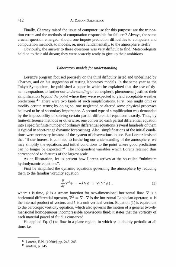
First he simplified the dynamic equations governing the atmosphere by reducingthem to the familiar vorticity equation
∂
∂t∇2ψ = −k∇ψ × ∇(∇2ψ) , (1)
where t is time,ψ is a stream function for two-dimensional horizontal flow,∇ is ahorizontal differential operator,∇2 = ∇ · ∇ is the horizontal Laplacian operator,× isthe internal product of vectors andk is a unit vertical vector. Equation (1) is equivalentto the barotropic vorticity equation, which also governs the motion of a general two-di-mensional homogeneous incompressible nonviscous fluid; it states that the vorticity ofeach material parcel of fluid is conserved.
He applied Eq. (1) to flow in a plane region, in whichψ is doubly periodic at alltime, i.e.
45 Lorenz, E.N. [1960c], pp. 243–245.46 Ibidem, p. 245.

Models in Meteorology (1946–1963) 413
ψ(x + 2π/k, y + 2π/l, t) = ψ(x, y, t) , (2)
where thex andy axes point eastward and northward, respectively, andk and l arespecified constants. In this way he distorted the geometry of the spherical earth, but heretained the important property that the effective area is finite but unbounded. He alsoneglected the horizontal variations of the Coriolis parameter, although Eq. (1) is stillconsistent with a constant Coriolis parameter.
Taking the Fourier transform of (1), and after some further substitutions introducingthe termsK,H , andM, Lorenz found the equations
dCM
dt= −
∑H
K ·H ×M
H ·H CHCM−H (3)
which is actually the infinite set of ordinary differential equations which he sought todetermine. The coefficientsCM are the dependent variables; as Lorenz explains, a fur-ther simplification is the omission of reference to all but a finite number of variablesCM corresponding to a specified set of values ofm andn. If these values are small, onlylarge-scale features are retained. The summation in (3) becomes a finite sum, but theequations are otherwise unaltered.
Equation (3) may be regarded as describing a nonlinear interaction between the com-ponents whose coefficents areCH andCM−H , to alter a third coefficientCM . Lorenzwanted to seek themaximum simplificationof (3) which still describes this process. Henoticed (but we don’t give here his proof) that clearly at least three terms with differenteigenvalues must be retained.
Finally, the governing equations, obtained either from (3), (or directly by some sub-stitutions into (1)), are written in the form:
dA
dt=
(1
k2− 1
k2 + l2
)klFG , (4)
dF
dt=
(1
l2− 1
k2 + l2
)klAG , (5)
dG
dt= −1
2
(1
l2− 1
k2
)klAF , (6)
A,F,G appear in the Fourier’s series ofψ and the coefficients ofFG,AG andAF areactually determined by the ratiok/l. The mean kinetic energy and the mean square ofthe vorticity,
E = 1
4
(A2
l2+ F 2
k2+ 2G2
k2 + l2
), (7)
and
V = 1
2
(A2 + F 2 + 2G2
); (8)
are readily seen to be conserved under Eqs. (4)–(6).

414 A. Dahan Dalmedico
According to Lorenz, these equations presumably contain the minimum number ofdegrees of freedom required to picture nonlinear barotropic phenomena. Lorenz calledthem the “minimum hydrodynamic equations”, or simply the minimum equations.47
Lorenz was aware that, when partial differential equations were numerically integrat-ed by means of finite differences in space and time, the phenomenon ofcomputationalinstabilitymight arise. In order to avoid such instability, the time interval�t should notto be too large compared with the space intervals�x and�y: when using orthogonalfunctions, the corresponding condition for computational stability was that�t shouldnot be too large a fraction of the oscillation period of the most rapidly oscillating vari-able. The simplified equations were realistic enough to provide a qualitative descriptionof some of the important physical phenomena in the atmosphere; they even led to plau-sible hypotheses concerning phenomena as yet not explained. According to Lorenz, thedegree of simplification, which one was permitted to use depended upon the particularphenomena one wished to investigate.
Lorenz developed different examples of “maximum simplification” of the system ofequations in order to investigate the following problems:
– The behavior of a jet under barotropic flow or its splitting into two streams.– Simple baroclinic flow. In this case, he said, one of the two-layer numerical predic-
tion models could be used instead of the barotropic vorticity equation. The maximumallowable simplification would then retain three degrees of freedom for the flow ineach layer, hence a total of six dependent variables. With such a system, the instabilityof zonal baroclinic flow could, among other phenomena, be studied.
– Forced baroclinic flow such as that which characterized the general circulation of theatmosphere.
All these simplifications might appear as rather crude approximations, Lorenzclaimed, but they should clarify our understanding of the phenomena and lead to plausi-ble hypotheses which might then be tested by means of careful observational studies andmore refined systems of dynamic equations. By judiciously omitting certain terms inthe dynamical equations and by comparing the result of the prediction with reality, onecould estimate the cost of these omissions and thereby decide which terms were impor-tant and which were not. We have here an explicit and complete description of what is, inLorenz’s mind, the right practice of modeling. A few years later, this conception would belargely considered as the canonical conception of modeling with computer simulations.Remarkably, that practice of modeling didn’t emerge spontaneously or immediately. Onthe contrary, it was object of much trial and error and many discussions.
At the same time, other meteorologists such as N.A. Phillips (also from MIT) wenton with their Sisyphean work.48 Also published in 1960, Phillips’s paper illustrated themethods in use at the time. He discussed the advantages of primitive equations overthe geostrophic model where wind is independent of the vertical coordinate; he alsomentioned a method for reducing initial noise. Phillips’s and the whole community’sefforts were not in vain, contributing, for instance, to the improvement of the quality
47 Lorenz [1960c], p. 247.48 Phillips, [1960].

Models in Meteorology (1946–1963) 415
of numerical integration. The two approaches which may be associated with Phillips’sand Lorenz’s names respectivly, that of physical models and that of laboratory models,proved useful.
In 1962, Charney gave a very good summary of the alternative: when faced withnonlinear problems, scientists will “choose either a precise model in order to predict oran extreme simplification in order to understand”.49 In his paper, Charney himself chosethe second alternative: he modeled whirlwinds with points, like Fermi, Pasta, and Ulamhad done at Los Alamos in 1947 when they modeled a rope by 64 punctual masses.50
Very simple and nonlinear, his system reproduced several whirlwinds around a circle andshowed their extreme instability. But Charney attributed the instability of the model torepeated truncation errors which would play the role of a disruptive force. Charney stillthought that a better computation would overcome that difficulty. This was very far fromthe point of view of Lorenz who had intuited that a small error could be self-amplifiedby the system even if one had exact computations at one’s disposal.
Encountering chaos
Barry Saltzman, from the Travelers Weather Center at Hartford, Connecticut, un-derstood the importance of Lorenz’s ideas. Instead of global atmospheric circulation,Saltzman studied the convective motion of a fluid heated from below, a very frequentatmospheric phenomenon which for example may locally occur over warm grounds. Forthis, he developed in 1961 a simple model involving 7 variables.51 He then made twoobservations which were to make his model famous. First, he noticed that in simulations4 of the 7 variables quickly became very small, and solutions flattened on the 3 others.Second, aside from regular solutions, he pointed out one that wasaperiodic. After havingpaid a visit to Saltzman, Lorenz became convinced that these 3 variables were keepingeach other going and that a system involving only 3 variables might well exhibit thesame behavior.
Let us enter in details. Rayleigh [1916] studied the flow occurring in a layer of flu-id of uniform depthH , when the temperature difference between the upper and lowersurfaces is maintained at a constant value�T . Such a system possesses a steady-statesolution in which there is no motion, and the temperature varies linearly with depth.If this solution is unstable, convection should develop. In the case where all motionsare parallel to thex–z plane, and no variations in the direction of they-axis occur, thegoverning equations had been written by Saltzman in the following form:52
∂
∂t∇2ψ = −∂(ψ,∇2ψ)
∂(x, z)+ υ∇4ψ + gα
∂θ
∂x, (9)
∂
∂tθ = −∂(ψ, θ)
∂(x, z)+ �T
H
∂ψ
∂x+ k∇2θ . (10)
49 Charney, [1962b], p. 289.50 Fermi, Pasta & Ulam [1947], in Ulam [1974].51 Saltzman [1962].52 Lorenz, [1963], p. 135. We refer here to Lorenz quoting Saltzman.
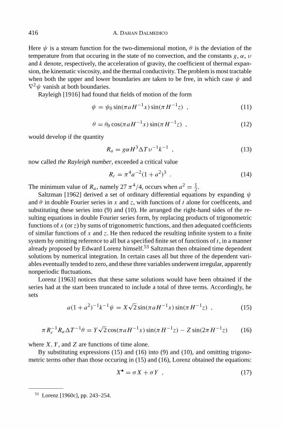
416 A. Dahan Dalmedico
Hereψ is a stream function for the two-dimensional motion,θ is the deviation of thetemperature from that occuring in the state of no convection, and the constantsg, α, υandk denote, respectively, the acceleration of gravity, the coefficient of thermal expan-sion, the kinematic viscosity, and the thermal conductivity. The problem is most tractablewhen both the upper and lower boundaries are taken to be free, in which caseψ and∇2ψ vanish at both boundaries.
Rayleigh [1916] had found that fields of motion of the form
ψ = ψ0 sin(πaH−1x) sin(πH−1z) , (11)
θ = θ0 cos(πaH−1x) sin(πH−1z) , (12)
would develop if the quantity
Ra = gαH 3�T υ−1k−1 , (13)
now calledthe Rayleigh number, exceeded a critical value
Rc = π4a−2(1 + a2)3 . (14)
The minimum value ofRa , namely 27π4/4, occurs whena2 = 12.
Saltzman [1962] derived a set of ordinary differential equations by expandingψ
andθ in double Fourier series inx andz, with functions oft alone for coefficents, andsubstituting these series into (9) and (10). He arranged the right-hand sides of the re-sulting equations in double Fourier series form, by replacing products of trigonometricfunctions ofx (or z) by sums of trigonometric functions, and then adequated coefficientsof similar functions ofx andz. He then reduced the resulting infinite system to a finitesystem by omitting reference to all but a specified finite set of functions oft , in a manneralready proposed by Edward Lorenz himself.53 Saltzman then obtained time dependentsolutions by numerical integration. In certain cases all but three of the dependent vari-ables eventually tended to zero, and these three variables underwent irregular, apparentlynonperiodic fluctuations.
Lorenz [1963] notices that these same solutions would have been obtained if theseries had at the start been truncated to include a total of three terms. Accordingly, hesets
a(1 + a2)−1k−1ψ = X√
2 sin(πaH−1x) sin(πH−1z) , (15)
πR−1c Ra�T
−1θ = Y√
2 cos(πaH−1x) sin(πH−1z)− Z sin(2πH−1z) (16)
whereX, Y , andZ are functions of time alone.By substituting expressions (15) and (16) into (9) and (10), and omitting trigono-
metric terms other than those occuring in (15) and (16), Lorenz obtained the equations:
X• = σX + σY , (17)
53 Lorenz [1960c], pp. 243–254.

Models in Meteorology (1946–1963) 417
Y • = XZ + γX − Y , (18)
Z• = XY − bZ . (19)
Here a dot denotes a derivative with respect to the dimensionless timeτ = π2H−2(1+a2)kt , while σ = k−1υ is thePrandtl number, r = R−1
c Ro, andb = 4(1 + a2)−1.Equations (17), (18), and (19) are the convection equations whose solutions Lorenzstudied.
In these equationsX is proportional to the intensity of the convective motion, whileY is proportional to the temperature difference between the ascending and descendingcurrents, equal signs ofX andY denoting that warm fluid is rising and cold fluid isdescending. The variableZ is proportional to the deviation of the vertical temperatureprofile from linearity, a positive value indicating that the strongest gradients occur nearthe boundaries.
Lorenz emphasizes that Eqs. (17)–(19) may give realistic results when the Rayleighnumber is slightly supercritical, but, in view of the extreme truncation, their solutionscannot be expected to resemble those of Salzman’s equations (9) and (10) when strongconvection occurs. Lorenz coded this system of 3 equations involving 3 variables formachine computing. Just as Saltzman had discovered with his model, Lorenz observedthe lack of periodicity for some solutions.54
Before he was hired as a meteorologist during World War II, Lorenz had been passion-ate about mathematics and had even contemplated a career in this field. With Saltzman’ssystem, he was allowed to go back to his first love. In order to interpret his results, Lorenzdove into Poincare’s and Birkhoff’s works and wrote a first version of an article aboutwhich nothing unfortunately is known today. An unknown referee directed him, not sur-prisingly, to Solomon Lefschetz’s books and, luckily for him, to the recent translationof Niemytskii and Stepanov’s book which covered the qualitative theory of dynamicalsystems developed by Alexandr Andronov’s Soviet school.55 There, Lorenz realized,was a set of elementary theoretical tools for the analysis of his results. In his seminalpaper published in 1963, Lorenz proved, after a brief introduction linking his problemto meteorology, that almost all solutions to his system of 3 equations (which he studiedin phase space) were unstable.56 If periodic solutions, of which there was a countableinfinity, were unstable, then quasiperiodic solutions could not exist. In his system, irreg-ular unstable trajectories were the general case. Hence a fundamental problem emerged:if nonperiodic solutions were unstable, two neighboring trajectories would diverge veryquickly. Otherwise, the “attractor”, which according to Lorenz was the portion of phasespace to which solutions tended, would have to be confined in a three-dimensional bowl;forcing two trajectories to come back very close to one another. Together with the re-quirement that two solutions cannot intersect, these constraints led Lorenz to imagine avery special structure for his attractor: an infinitely folded surface, the “butterfly” that
54 See Lorenz [1993], pp. 136–160.55 About the development of dynamical systems in the 1950s and 1960s and the diffusion of
Soviet results see Dahan Dalmedico [1994] and [1997].56 Lorenz [1963] pp. 130–141.

418 A. Dahan Dalmedico
has now become very familiar. Representing the attractor in terms of a two-dimensionalprojection, Lorenz used Poincare’s first-return map in order to study his attractor better.
The conclusions drawn by Lorenz in his paper were twofold: (1) From a theoreti-cal standpoint, he proved that very complicated behaviors could arise from very simplesystems – simplicity could generate complexity, in contradiction to the old, well-estab-lished conviction that simple causes should give rise to simple effects. And (2) he alsoexhibited the property of sensitivity to initial conditions and thus opened a window onthe understanding of turbulence. At the meteorological level (provided his model hadanything to do with the atmosphere), hopes for long-range predictions were doomed.The old debate about whether a larger number of degrees of freedom would stabilizethe system, or not, was put to rest. In this perspective, all that remained for Charney towork on was to try discovering the limits for effective prediction.
The aftermath of Lorenz’s work goes beyond the scope of this paper; I shall notdeal with the mathematical apprehension of these results; how mathematicians graspedthem, how different communities (meteorologists, mathematicians, but also physicists,specialists of fluid mechanics, and population biologists) came to meet each other arounda few similar issues. Let me simply mention that, published in theJournal of Atmospher-ic Sciences, Lorenz’s paper remained unnoticed by mathematicians until 1972. At leastthree times, Lorenz’s results failed to attract the mathematical community’s attentionwhen they might have.57 First, one of the referees asked to evaluate Lorenz’s paper wasnone other than Stan Ulam. Having carefully studied with Stein at Los Alamos, theiteration of nonlinear functions and having been involved in the famous Pasta-Fermi-Ulam experiment, he should have been, one may think, sensitive to these issues. But,too busy at the time, he entrusted the job to a colleague. Secondly, meeting Ulam around1965, Lorenz mentioned his research without showing him his attractor; this again wasnot enough to catch the mathematician’s attention. Finally, at a meeting on “Statisti-cal Methods and Turbulence” in 197158, Ruelle gave a short talk about a mathematicalexplanation for the onset of turbulence (regarded as a bifurcation problem) and brieflyexpounded what became known later as his strange attractor theory. Participating in thesame session at this symposium, Lorenz remarkably was the only one, apart from Ruellehimself, who shunned stochastic processes and statistical methods and was rather moreinterested in the prediction of what he called “models” of turbulence.59 A modest, shyman who belonged to a scientific community different from Ruelle’s, Lorenz preferredto wait until he could check his own results before mentioning that his earlier work of1963 perfectly corresponded to what he had just heard from the mathematical physicist.Once more, an opportunity was missed to call other scientists’ attention to his work. Butthis time, he would not have to wait for long before fame would catch up with him.
57 Personal Interview with the author (Boston, Mai 1992).58 Ruelle [1971].59 Lorenz [1971], p. 195, where he wrote: “Ensembles of solutions of simplified or ortherwise
modified forms of the Navier-Stokes equations will not qualify as turbulence; we shall insteadregard them as models of turbulence”.

Models in Meteorology (1946–1963) 419
Concluding remarks
Returning to the epistemological issues pertaining to the question of models andmodeling raised at the beginning of this paper, we realize that contemporary modelingpractice takes place between two poles: one is operational and linked to prediction, theother is turned towards cognition, explanation, and understanding. Although examinedhere for the specific case of meteorology, this duality is a very general feature. Thefirst pole played the major role in 1946–55, the second one became dominant around1960; nevertheless, they coexisted and intermingled throughout both periods. Moreover,although protagonists often spoke simply of therepresentativeness of a model, it is clearthat the confrontation does not rest upon a reality supposed as being already there anda model which would represent it. It is not reality which is represented but already asubtle and complexreconstruction, both theoretical and empirical, of this reality. Thereconstruction takes place on several levels: (1) a system of hypotheses, theories, andconcepts, which are both fundamental principles and simplifying assumptions; (2) asystem of observations and measurements; and (3) objectives and norms of prediction,efficiency, and uses. None of these levels is obvious and transparent. In the case wefollowed here, the first level mobilized general laws of physics (laws of motion, con-servation of energy, the Navier-Stokes equations, and other hydrodynamic concepts),but also a whole set of assumptions allowing for the reduction of the system of equa-tions into simplified forms (geostrophic equation or balance equations, for instance).On the second level, a statistically and cartographically complex device of observations,measurements, and interpolations intervened. The third level was linked with what me-teorologists are presently confronting: the fact that modeling of the atmosphere dependson whether one makes one or two-day weather forecasts, studies the evolution of atyphoon or a jet-stream, or investigates climate change.
In conclusion, this story underlines the crucial importance of numerical simulations:by isolating different factors and evaluating their respective roles, computer and nu-merical experiments as well as laboratory models gave rise to a better exploration andunderstanding of “reality”. We have also noted the role of numerical methods and thedifficulties related to different kinds of algorithms for the integration or discretization ofequations at the different points of the lattice (in particular, the determination of time-and space-steps satisfying the Courant condition). In testing models for predicting atmo-spheric phenomena, failures may have their origin either in each of the levels mentionedabove, or in computing methods and truncation errors, or in the phenomenon itselfre-gardless of the way in which it has been modeled. But, confronted with unpredictablebehavior and instability, it is almost impossible to affirm whether or not they arise fromtheontologyof the phenomenon. Even after Lorenz’s results, a few clung to hopes forbigger models and the question was not definitively settled.
In the field of meteorology, the introduction of the mathematical theory of dynamicalsystems came after that of modeling practices. One may remark that this process wasrather the opposite to what happened with Ruelle and his followers, who delved into theturbulence problem by means of qualitative dynamics, only to turn later to simulations asa direct result of their acceptance of Lorenz’s system. Modeling practices, however, werehardly foreign to fluid mechanicists, but because of the field’s much greater simplicitycompared with atmospheric motions, the question of the (linear) stability of dynamical

420 A. Dahan Dalmedico
equations in pure hydrodynamics was solvable by means of a combination of numericaland analytic methods. While in the latter case, modeling practices remained subservientto the analytical problems, meteorologists tackled the very issue of stability by means ofcomputer simulations. Conversely, it was the wider understanding of chaotic dynamicswhich gradually led meteorologists to adopt an approach inspired by dynamical systemstheory.
From the early computing machines to giant calculators, the computer was employedin a variety of ways in fluid geophysics. Identifying four types of computer usage be-tween 1945 and 1972, Charney used the terms synthetic, experimental, heuristic, anddata-analytic:
According to this classification, a computer’s operation issyntheticwhen it is used topredict or stimulate large-scale phenomena.Experimentaluse occurs when the computersimulates an individual phenomenon, in isolation from its environment, so that the usermay infer its physical causes. The computer is usedheuristicallyto build highly simplifiedmodels as a means to discover new relationships in the atmosphere. Finally the computercan be used toreduce and analyzeobservational data.60
Concerning the Meteorological Project, one may state that the work on general cir-culation wassynthetic, whereas the use of simple baroclinic models to determine thephysical basis of cyclogenesis wasexperimental. The arguments above imply that theheuristic use of computers took off only in the early 1960s, largely on the basis ofSaltzman’s and Lorenz’s work on maximum simplification models.
Acknowledgments.This paper has benefited greatly from the editorial comments from the editorsof theArchive, especially Henk Bos. I wish to express to them my gratitude.
References
Aspray, W. [1988] “The Emergence of Princeton as a World Center for Mathematical Research”,1896–1939, inHistory and Philosophy of Modern Mathematics, William Aspray and Phil-ip Kitcher, (ed.), Minnesota Studies in the Philosophy of Science, vol. 11, Minneapolis:University of Minnesota, 346–66.[1990] John von Neumann and the origins of modern computing, Cambridge (MA), MIT
Press.Bigelow, J. [1980] “Computer development at the Institute for Advanced Study”, inA History
of computing in the Twentieth Century, N. Metropolis, J. Howlett and G.C. Rota, (eds.),Academic Press, New York, 291–310.
Birkhoff, G. [1977] “Applied mathematics and its future”, in Thomson, R.W., (ed.),Science andtechnology in America, NBS, publ. 465.[1980] Computing developments 1935–1955, as seen from Cambridge, U.S.A., in “A His-
tory of Computing in the Twentieth Century”, N. Metropolis, J. Howlett and G.C. Rota (eds.),Academic Press, New York, 21–30.
Charney, J. [1955] “Numerical Methods in Dynamical Meteorology”,Proceedings of the NationalAcademy of Science41, 11 (November), 798–802; quoted in Aspray [1990], 152–153.
60 Charney [1972], p. 121, quoted in Aspray [1990], p. 153.

Models in Meteorology (1946–1963) 421
[1960] “Numerical prediction and the general circulation”, inDynamics of Climate, R.L.Pfeffer (ed.), Pergamon, New York, 12–17.[1962a] “Integration of the Primitive and Balance Equations”,Proceedings Internation-
al Symposium on Numerical Weather Prediction in Tokyo, November 1960, pub. in 1962,131–152.[1962b] “Numerical experiment in atmospheric hydrodynamics”,Proceedings of Sympo-
sium in Applied MathematicsXV, p. 289.[1972] “Impacts of Computers on Meteorology”,Comput. Phil. Commun., 3, Suppl., 117–
126.Charney, J., Fjortoft, R. and von Neumann, J. [1950] “Numerical integration of the barotropic
vorticity equation”,Tellus, 2, 237–254.Courant, R., Friedrichs, K. and Lewy, H. [1928] “Uber die partiellen Differenzengleichungen der
Mathematischen Physik”,Mathematische Annalen, 100, 32–74.Cvitanovic, P. [1984]Universality in Chaos: a Reprint Selection, Bristol, Adam Hilger.Dahan Dalmedico, A. [1994] “La renaissance des systemes dynamiques auxEtats-Unis apres la
deuxieme guerre mondiale: l’action de Solomon Lefschetz”,Supplemento ai Rendiconti delCircolo matematico di Palermo, II, 34, 133–166.[1997] “Le difficile heritage de Henri Poincare en systemes dynamiques”, in Greffe, J.,
Heinzmann, G., & Lorenz, K., (eds.),Henri Poincare, science et philosophie, Berlin, Ak-ademie Verlag & Paris, Blanchard, 13–33.[1996] “L’essor des mathematiques appliquees aux Etats-Unis: l’impact de la seconde
guerre mondiale”,Revue d’Histoire des Mathematiques, 2 (1996), 149–213.[1997] “Mathematics in the 20th century”, in Krige, J. & Pestre, D., (eds.),Science in the
20th century, London, Harwood Academic Publishers, 651–667.[1999] “Pur versus applique? Un point de vue d’historien sur une ‘guerre d’images’ ”,
La Gazette des mathematiciens, Publication de la Societe Mathematique de France, n◦ 80,31–46.[forthcoming] “Chaos, Disorder and Mixing: A new ‘Fin de siecle’ Image of Science?”, to
appear inGrowing Explanations, N. Wise (ed.), Princeton University Press.[in press] “An Image Conflict in Mathematics after World War II”, in Bottazzini, U. &
Dahan Dalmedico, A. (eds),Changing Images in Mathematics. From the French Revolutionto the new Millenium, Harwood. Acad. Publ., London.
Fermi, E., Pasta, J. and Ulam, S. [1947],Studies of non-linear problems(Los Alamos Document),published in Ulam [1974],Sets, Numbers and Universes, Selected Papers, (Cambridge, MIT-Press).
Goldstine, H.H. [1972]The Computer from Pascal to von Neumann, Princeton University Press,Princeton, NJ.[1977]A history of Numerical Analysis from the 16th through the 19th Century, Springer-
Verlag, New York.Heims, S.J. [1980]John von Neumann and Norbert Wiener. From mathematics to the technologies
of life and death, Cambridge (MA), MIT-Press.Lorenz, E.N. [1960a] “Energy and Numerical Prediction”,Tellusn◦ 12, 364–373.
[1960b] “The Statistical Prediction of Solutions of Dynamic Equations”,Proceedings In-ternational Symposium on Numerical Weather Predictionin Tokyo, 629–635.[1960c] “Maximum Simplification of the Dynamic Equations”,Tellus12, n◦ 3, 243–254.[1963] “Deterministic non periodic flow”,Journal of Atmospheric Sciences, 20, n◦ 2, 130–
141.[1970] “The nature of the global circulation of the atmosphere: A present view”, The Global
Circulation of the Atmosphere, G.A. Corby (ed.),Meterol. Soc., London, 2–23.[1993]The Essence of Chaos, Seattle, University of Washington Press.

422 A. Dahan Dalmedico
Metropolis, N., Howlett, J. and Rota, G.C. (eds.),A History of computing in the Twentieth Century,Academic Press, New York, 291–310.
Nebeker, F. [1995]Calculating the Weather. Meteorology in the 20th Century, San Diego, Aca-demic Press.
Nemytskii, V.V. and Stepanov, V.V. [1960]Qualitative theory of differential equations, Princeton,Princeton Univ. Press.
Neumann, J. von. and Richtmyer, R.D. [1950] “A method for the numerical calculation of hy-drodynamic shocks”,Journal of Applied Physics, 21, 232–237; von NeumannWorksVI,380–385.
Phillips, N.A. [1951] “A simple three-dimensional model for the study of large-scale extratropicalflox patterns”,J. Meteorol. Soc., 8, 381–394[1960] “Numerical Weather Prediction” inAdvances in Computers, New York Academic
Press.[1960] “On the Problem of initial fluid data for the primitive equations” (1959)Tellus12,
n◦ 2.Platzman, G.W. [1952] “Some remarks on high-speed automatic computers and their use in me-
teorology”,Tellus, 4, 168–178.[1967] “A retrospective view of Richardson’s book on weather prediction”,Bull. Am. Me-
teorol. Soc., 48, 514–550.[1979] “The ENIAC computations of 1950 – gateway to numerical weather prediction”,
Bull. Am. Meteorol. Soc., 60, 302–312.Proceedings Third Berkeley Symposium of Mathematical Statistics, [1955], vol I, II, III, IV.Proceedings International Symposium on Numerical Weather Prediction in Tokyo, November
1960, [1962] ed. Sigekata Siono (1962). Tokyo: Meteorological Society of Japan.Rayleigh, Lord [1916] “On convective currents is a horizontal layer of fluid when the higher
temperature is on the under side”,Phil. Mag., 32, 529–546.Ruelle, D. [1980] “Strange Attractors”,Math. Intelligencer, 2, n◦ 126, 37–48.Saltzman, B. [1962] “Finite amplitude free convection as an initial value problem”,Journal of
Atmospheric Sciences19, 329–341.[1967] “Meteorology: A brief history”, inEncyclopedia of Atmospheric Sciences and Astro-
geology, R.W. Fairbridge (ed.), Reinhold, New York, 583–591.Smagorinsky, J. [1983] “The beginnings of numerical weather prediction and general circulation
modeling: Early recollections”,Adv. Geophys., 25, 3–37.Thompson, P. [1983] “A history of Numerical Weather Prediction in the United States”,Bulletin
of The American Meteorological Society, 64, 7, 755–769.Wiener, N. [1956] “Nonlinear Prediction and Dynamics”,Proc. 3rd Berkeley Sympos. Math. Stat.
and Prob., 247–252.
Centre Alexandre KoyreCNRS
57 Rue Cuvier (Pavillon Chevreuie)75005 Paris
(Received February 11, 2000)