Embed Size (px)
Citation preview
HIV/AIDS impact on childhood mortality and childhood mortality measurement: from the
perspective of Kenyan and Malawian DHS data
Chifundo Kanjala
Thesis submitted in partial fulfillment for
the Degree of Master of Philosophy in Demography
in the Faculty of Commerce, University of Cape Town
August 2008
2
Plagiarism declaration form
This research is my original work, produced with normal supervisory assistance from
my supervisor. All the relevant sources of knowledge that I have used during the course
of writing this dissertation have been fully credited using the Harvard convention for
citation and referencing. Also, this dissertation has not been submitted for any academic
or examination purpose at any other university.
--------------------------------------- ----------------------
Chifundo Kanjala Date

3
Dedication
To my sweet mum, whose love is my inspiration.
4
Abstract This study has two goals. The first is to assess the consistency of the childhood
mortality trends constructed from the direct and the indirect methods of estimation in
high HIV prevalence settings. The second goal is to assess the direct impact of
HIV/AIDS on childhood mortality in Kenya and Malawi for the periods 1999 – 2003
and 2000 – 2004 respectively.
It is important to understand the impact of HIV on childhood mortality and
childhood mortality measurement to ensure that child health planning and evaluation
are correctly informed.
Trends of infant and under-five mortality are constructed for each country by
applying the Brass Children Ever Born Children Surviving method to census and
Demographic and Health Survey (DHS) data collected in the HIV/AIDS era (1992 –
2004). Trends of childhood mortality are also constructed using direct childhood
mortality estimates obtained from applying the synthetic cohort life table analysis to
DHS data.
To assess the impact of HIV on childhood mortality, the proportions of
childhood mortality attributable to HIV (HIV PAF) in the five year periods leading to
the Kenyan 2003 and the Malawian 2004 DHS are estimated using DHS birth histories
data and results from African longitudinal studies involving paediatric HIV infection
and survival.
The results from the trend analysis reveal that the trends of childhood mortality
from the direct and the indirect methods applied to Kenyan and Malawian DHS data
are different. While the direct estimates generally give well defined trends, the trends
from the indirect estimates are erratic. However, being less erratic does not confirm the
correctness of the trends from the direct method since it is possible for the trends to be
biased to the same extent and in the same direction.
The HIV PAFs obtained are 5.3 per cent (Kenya) and 6.8 per cent (Malawi) for
infant mortality and 14.3 per cent (Kenya) and 18.0 per cent (Malawi) for under-five
mortality respectively. As expected, the impact of HIV is higher on under-five mortality
than it is on infant mortality in both Kenya and Malawi. The results also suggest that
Malawi had higher proportions of mortality attributable to HIV/AIDS compared to
Kenya. The uncertainty surrounding the PAFs however makes it impossible to say the

5
difference is material. The PAFs are also lower than what would be expected. Since the
methodology used has given inconsistent results of HIV PAF, it is recommended that
further improvements be made to the estimates of HIV PAF and their sensitivity to
changes in the inputs be assessed before they can be used for any decision making on
HIV impact reduction.

6
Acknowledgements
First and foremost, I thank God, the Almighty for sustaining me as I was working on
my thesis.
I acknowledge that there are quite a few people who contributed towards the successful
completion of this piece of work. I would like to thank my supervisor, Dr Tom Moultrie for his patience and tireless
efforts in guiding me from the beginning of my project to the end. I thank Professor
Rob Dorrington who advised me on a major section of my thesis. I thank my fellow
students at the Centre for Actuarial Research (CARe) for their continual support and
friendship.
I also thank family members and friends who supported me financially and emotionally.
Their support was invaluable as I went through this potentially lonely exercise. These
include Tawanda, Samson, Lazarous, Lawrence, Pardon, Ntsoaki, Bronwyn who proof-
read drafts of my project, Martin, Ronnie, Nico, my church Life Group and many
others too numerous to mention.
Last but not least, I thank the funders of my Masters studies, the Andrew W Mellon
Foundation, for providing the funding I used for fees and other living expenses during
my studies.
7
Table of contents
Plagiarism declaration form ................................................................................... 2
Dedication .............................................................................................................. 3
Abstract ................................................................................................................... 4
Acknowledgements ................................................................................................ 6
Table of contents .................................................................................................... 7
List of tables ........................................................................................................... 9
List of figures ......................................................................................................... 10
1. Introduction ................................................................................................... 11
1.1. Background .............................................................................................................. 11
2. Literature Review........................................................................................... 14
2.1. Introduction ............................................................................................................. 14
2.2. Measures of childhood mortality .......................................................................... 14
2.3. Data sources ............................................................................................................. 15
2.4. Methods for estimating childhood mortality ...................................................... 15
2.5. Consistency and use of childhood mortality estimates in Africa ..................... 21
2.6. Problems with the traditional methods of childhood mortality measurement
in high HIV prevalence settings prevailing in African countries ..................... 23
2.7. Understanding the effect of HIV on childhood mortality ................................ 24
2.8. New approaches to childhood mortality measurement .................................... 27
2.9. Conclusion ............................................................................................................... 31
3. Data ............................................................................................................... 34
3.1. Introduction ............................................................................................................. 34
3.2. Background information on Kenya and Malawi ................................................ 34
3.3. Data sources ............................................................................................................. 35
3.4. Data quality .............................................................................................................. 37
3.5. Conclusion ............................................................................................................... 49
4. Comparison of childhood mortality trends .................................................. 50
4.1. Introduction ............................................................................................................. 50
8
4.2. Trends of direct and indirect estimates of childhood mortality ....................... 50
4.3. Comparison of trends from the direct and the indirect methods .................... 57
4.4. Conclusion ............................................................................................................... 60
5. HIV population attributable fraction (PAF) ................................................. 61
5.1. Introduction ............................................................................................................. 61
5.2. Overall childhood mortality .................................................................................. 61
5.3. Mortality of uninfected children ........................................................................... 62
5.4. Estimation of the proportions of childhood mortality attributable to
HIV/AIDS (HIV PAF) ......................................................................................... 69
5.5. Conclusion ............................................................................................................... 70
6. Discussion and conclusions .......................................................................... 71
6.1. Introduction ............................................................................................................. 71
6.2. Childhood mortality trends from the direct and the indirect methods ........... 71
6.3. HIV/AIDS attributable childhood mortality (HIV PAF) ................................ 73
6.4. Limitations of the study ......................................................................................... 75
6.5. Conclusions and recommendations ..................................................................... 76
References ............................................................................................................ 79
Appendix .............................................................................................................. 85
9
List of tables
Table 2.1 HIV PAF results from some African longitudinal studies ........................... 26 Table 3.1 DHS datasets and data collection periods ...................................................... 35 Table 3.2 Basic demographic characteristics of Kenyan women aged 15-49 from
various data sources ........................................................................................... 40 Table 3.3 Average parities by education of Kenyan women (15-49), various sources .. ............................................................................................................................... 43 Table 3.4 Sex ratios of children ever born to Kenyan women aged 15-49 ................. 44 Table 3.5 Basic demographic characteristics of Malawi women aged 15-49 from
various sources .................................................................................................... 46 Table 3.6 Average parities by education level of Malawian women (15-49), various
sources .................................................................................................................. 48 Table 3.7 Sex ratios of children ever born to Malawian women age 15-49 ................ 49 Table 4.1 Direct childhood mortality estimates for Kenya .......................................... 52 Table 4.2 Direct childhood mortality estimates for Malawi .......................................... 52 Table 4.3 Indirect childhood mortality estimates for Kenya ......................................... 55 Table 4.4 Indirect childhood mortality estimates for Malawi ........................................ 56 Table 5.1 overall childhood mortality and the mortality of the children of uninfected
mothers ................................................................................................................ 62 Table 5.2 Mortality of HIV-exposed children and children of HIV negative mothers
from African longitudinal studies..................................................................... 63 Table 5.3 Mortality ratios comparing mortality of the two groups of uninfected
children................................................................................................................. 64 Table 5.4 Mortality ratios and childhood mortality of HIV-exposed children ........... 65 Table 5.5 Numbers of women giving birth and the DHS age-specific prevalence rates ............................................................................................................................... 66 Table 5.6 Sentinel surveillance based prevalence rates for Kenyan and Malawian
women (15-49) .................................................................................................... 67 Table 5.7 Adjusted HIV prevalence rates for Kenyan and Malawian women 15-49 . 67 Table 5.8 Contributions to mortality of uninfected children ........................................ 68 Table 5.9 Mortality of all uninfected children and HIV PAF for Kenya (1999-2003)
and Malawi (2000-2004) .................................................................................... 69
10
List of figures
Figure 3.1 Age distributions of Kenyan women aged 15-49, various data sources ..... 41 Figure 3.2 Average parities of Kenyan women (15-49), various data sources ............. 42 Figure 3.3 Age distributions of Malawian women (15-49), various data sources ........ 45 Figure 3.4 Average parities of Malawian women (15-49), various data sources .......... 47 Figure 4.1 IMR and U5MR trends in Kenya from the direct method .......................... 51 Figure 4.2 IMR and U5MR trends in Malawi from the direct method ......................... 53 Figure 4.3 IMR and U5MR trends in Kenya from the indirect method ....................... 55 Figure 4.4 IMR and U5MR trends in Malawi from the indirect method ...................... 56 Figure 4.5 Direct and indirect estimates of infant mortality for Kenya ........................ 57 Figure 4.6 Direct and indirect estimates of infant mortality for Malawi ....................... 58 Figure 4.7 Direct and indirect U5MR estimates for Kenya ............................................ 59 Figure 4.8 Direct and indirect U5MR estimates for Malawi ........................................... 59
11
1. Introduction
1.1. Background
The analysis of trends of mortality under the age of 5 (childhood mortality) in Africa
reveal that childhood mortality started declining in the second half of the twentieth
century (2000). The speed of decline reduced from around the mid 1980s in many
African countries. Some countries, for example Kenya, actually experienced a reversal
of trends (Central Bureau of Statistics (CBS) [Kenya], Ministry of Health (MOH)
[Kenya] and ORC Macro, 2004). As pointed out by Walker, Schwartlander and Bryce
(2002), HIV/AIDS has often been singled out as the major contributor to these adverse
trends. In addition to having an impact on the trends of childhood mortality,
HIV/AIDS is also said to be affecting the measurement of childhood mortality (Ward
and Zaba, 1999; Mahy, 2003).
It is important to understand the exact impact of HIV/AIDS on childhood
mortality and its measurement to ensure the accurate measurement of childhood
mortality in high HIV prevalence settings (estimated adult HIV prevalence greater than
5 per cent (Maher, Watt, Williams et al., 2005)). Accurate measurement of childhood
mortality is crucial since the childhood mortality estimates are used as indicators of
general social development and health (Hill, 1991).
Ideally, childhood mortality estimates should be derived from vital registration
systems and data on the population at risk from censuses or continuous population
registers. However, vital registration in Africa is uniformly incomplete and inaccurate
(United Nations, 1992; Cleland, 1996; Setel, Macfarlane, Szreter et al., 2007; UNICEF,
WHO, World Bank et al., 2007).
The absence of reliable vital registration has been compensated for by indirect
childhood mortality measurement using census data or direct childhood mortality
estimates derived from detailed birth histories provided by women of reproductive age
interviewed in household surveys.
The advent of the Human Immune Virus (HIV) which causes Acquired
Immuno-deficiency Syndrome (AIDS) has led to the violation of the assumptions on
which the methods used for childhood mortality measurement in Africa are based. This
has mainly been due to the retrospective nature of the data (Ward and Zaba, 1999;
12
Mahy, 2003). Retrospective reporting of children’s survival by mothers can only be
done by mothers who are alive at the time of the interview. Mothers who die between
giving birth and the time of the survey are not available to report on the death of their
children. The exclusion of the mortality of the children of deceased mothers may bias
childhood mortality estimates because these omitted children normally have higher
mortality than children in the general population (Nakiyingi, Bracher, Whitworth et al.,
2003; Newell, Brahmbhatt and Ghys, 2004).
Research has confirmed that HIV/ AIDS impacts childhood mortality (Nicoll,
Timaeus, Kigadye et al., 1994; Adetunji, 2000; Hill, Cheluget, Curtis et al., 2004). Efforts
have also been made to quantify the impact of HIV/ AIDS on childhood mortality
(Ward and Zaba, 1999; Zaba, Marston and Floyd, 2003; Marston, Zaba, Salomon et al.,
2005). However, more work still needs to be done to further our understanding of the
impact of HIV/AIDS on childhood mortality and childhood mortality measurement.
This project contributes towards further understanding of the direct impact of
HIV/AIDS on childhood mortality and its measurement.
The research has two aims. The first is to analyse the consistency of childhood mortality
estimates derived from the direct method of childhood mortality measurement and
those from the indirect method using data from Kenya and Malawi DHS surveys and
censuses done during the period 1990 to 2004.
The second aim is to quantify the direct impact of HIV/AIDS on childhood
mortality in the two above-mentioned countries in the five years before the Kenya 2003
DHS and the Malawi 2004 DHS.
The next chapter reviews the literature related to the project. It also specifies the gap in
the body of knowledge the project intends to fill.
Chapter 3 gives the sources of the data used in this study and an appraisal of
their quality. In chapter 4, the methodologies used to analyse the trends of childhood
mortality are described and the results obtained are presented. Trends in infant
mortality rates and under-five mortality rates from the direct and indirect methods are
examined and a comparison is made between the trends suggested by the direct and the
indirect methods. Chapter 5 presents the method used to assess the direct impact of
HIV/AIDS on childhood mortality and the results obtained from applying the method
to Kenyan and Malawian data. The last chapter (chapter 6) comprises of the discussion

13
of the results, the conclusions drawn from the data analysis and suggestions for future
research.
14
2. Literature Review
2.1. Introduction
This chapter reviews the literature on childhood mortality measurement in high HIV
prevalence settings prevailing in Africa. In particular the review will focus on the
traditional methods of measuring childhood mortality used in Africa, some of the
problems that arise from using these methods in high HIV prevalence settings and the
new approaches to childhood mortality measurement developed for high HIV
prevalence settings. The review will also point out the need for comparison of trends of
childhood mortality estimates from the direct and the indirect methods in high HIV
prevalence settings and the need for the use of relatively current, empirical and
nationally representative data for assessing the impact of HIV on childhood mortality.
Section 1A in the Appendix provides selected definitions of some concepts
related to childhood mortality and its measurement used (some repeatedly) in this
chapter.
2.2. Measures of childhood mortality
Mortality under the age of five can be broken down into neonatal mortality, post-
neonatal mortality, infant mortality and child mortality depending on the exact age at
death of the child. However, the infant mortality rate (IMR) and the under-five
mortality rate (U5MR) are the conventional measures of childhood mortality (Hill and
Amouzou, 2006). These two are chosen because of their characteristics. IMR
contributes the majority of under-five mortality (UNICEF, WHO, World Bank et al.,
2007). The mortality between age 1 and 5 is also substantial, especially in developing
countries (Population Division United Nations Secretariat, 1990); this makes the IMR
inadequate for fully describing of mortality in childhood.
The U5MR gives a good summary measure of mortality in childhood; it
captures almost all deaths in children under the age of 18 (United Nations, 1992;
UNICEF, WHO, World Bank et al., 2007). However, it is also important to monitor the
IMR because it captures increasingly larger proportions of U5MR as mortality of
children below the age of five declines. Therefore, it is best to monitor both U5MR and
IMR.
15
2.3. Data sources
The data for childhood mortality measurement in Africa come mainly from household
surveys. These household surveys include Demographic and Health Surveys (DHS),
Multiple Indicator Cluster Surveys (MICS) (UNICEF, WHO, World Bank et al., 2007)
and country-specific studies. MICS are usually conducted in countries that have not
done DHS surveys (Mahy, 2003). The household surveys provide data for both direct
and indirect mortality estimation.
The DHS data provide more detailed nationally representative birth histories
data than MICS. MICS only collect birth histories for the last three births from the
women interviewed. The quality of the DHS is considered the best of all household
surveys in Africa (Zaba, Marston and Floyd, 2003) in terms of being relatively error free
and nationally representative. Cluster sampling is used to obtain DHS samples. A typical
DHS interviews some 7000 women (Korenromp, Arnold, Williams et al., 2004).
Though census data are used for indirect childhood mortality estimation, data
from this source are not as frequently available as they are needed (UNICEF, WHO,
World Bank et al., 2007). The censuses are normally done at ten year intervals.
Censuses aim to enumerate the entire population in a country. They also cover
other socio-economic aspects of a population besides its demography. Thus, data on
childhood mortality collected in censuses are less detailed compared with those from
household surveys.
2.4. Methods for estimating childhood mortality
There are two main categories of childhood mortality estimation techniques. These are
the direct and the indirect methods. These two categories are based on different
assumptions and they have different data requirements. Detailed descriptions of these
two methods are given below.
2.4.1. Direct childhood mortality estimation
There are three approaches to direct estimation of childhood mortality. These are: the
vital statistics approach, the true cohort approach and the synthetic cohort approach
(Rutstein and Rojas, 2006).
2.4.1.1. The vital statistics approach
The vital statistics approach uses childhood deaths recorded in vital registration systems
and census data (or any other accurate estimates of the population) to estimate
childhood mortality. Data recorded in a reliable vital registration system can solely be
16
used for estimation of IMR. This is done by dividing deaths occurring within a year of
interest among children aged below one by the number of children born within that
year (Population Division United Nations Secretariat, 1990).
However, to estimate U5MR, data from the vital registration system are used
jointly with data from a national population census or data from a population register to
closely approximate the population exposed to risk of death. The U5MR is estimated as
the number of deaths below the age of five per 1000 births. Data from the vital
registration system cannot be relied upon for estimating the population at risk for use in
estimating the U5MR unless migration is captured in the vital registration system
(UNICEF, WHO, World Bank et al., 2007).
2.4.1.2. The true cohort approach
The second direct approach is the true cohort approach. Deaths to children of a specific
birth cohort are divided by the number of births in that cohort- the estimates obtained
do not refer to any particular period but rather to the mortality experiences of cohorts
as they progress through life (Rutstein and Rojas, 2006).
A birth cohort has to be observed for the full duration of time for which
estimates are required. For example, if under-five mortality estimates are required, a
birth cohort has to be observed for the full five years. Therefore, there is need for a lot
of time of observation which is usually not feasible and the longer the time horizon the
more out of date are the results.
Though the time constraints associated with following a birth cohort from
birth up to age five are not very serious (Population Division United Nations
Secretariat, 1990), there is still the disadvantage that this approach does not allow more
recent births to be included in the estimates since each person involved has to belong to
the birth cohort of interest, and not later cohorts (Rutstein and Rojas, 2006).
The true cohort approach has been applied mainly in some African longitudinal
surveys following birth cohorts usually for periods of up to two years (Crampin, Floyd,
Glynn et al., 2003). In some studies, the periods of follow up have however gone up to
five years (Spira, Lepage, Msellati et al., 1999).
2.4.1.3. The synthetic cohort approach
The third approach is to use synthetic cohorts. The survival experiences of children at
different ages collected during a cross-sectional survey are assumed to be an
approximation of what a real cohort would experience if the mortality rates prevailing
17
during the survey period were to remain unchanged over a specified time period
(Preston, Heuveline and Guillot, 2001).
The data needed for the synthetic cohort approach are the date of birth of each
child, the sex of the child, the child’s survival status at the time of the survey, the age at
survey or date of death, whichever is applicable at the time of the survey (Rutstein and
Rojas, 2006). The method also requires ages of the female respondents at the time of
the survey.
The children are classified into age groups for estimation of probabilities of dying.
The age groups are as follows: less than 1 month, 1 – 2 months, 3 – 5 months, 6 – 11
months, 12 – 23 months, 24 – 35 months, 36 - 47 months and 48 - 59 months (Rutstein
and Rojas, 2006). Alternative grouping of the children into segments one month long
were found to have no advantage over the grouping above. Using dates of births and
date of either death or interview, whichever comes first, numbers of children dying in
each of the above mentioned age groups and specific five year periods before the survey
are determined. The number of events of interest (deaths) in each of the age groups and
the time periods mentioned above are then calculated. The numbers of deaths in each
of the given age segments are divided by the numbers of survivors at the beginning of
each of the appropriate age intervals.
After obtaining the probabilities of dying within each of the segments given
above, probabilities of surviving are calculated as complements of the probabilities of
dying. The cumulative probabilities of dying at specific ages can then be calculated.
As mentioned before, specific mortality estimates of interest in this project are the
IMR and the U5MR. For further details on calculation of the other childhood mortality
measures (neonatal mortality rate and child mortality rate), the reader is referred to a
more detailed report on childhood mortality estimation prepared by Rutstein and Rojas
(2006).
Calculation of the IMR involves use of the cumulative probability of survival to
12 months; the product of survival probabilities up to 12 months is subtracted from 1.
The result is then multiplied by 1000 to obtain the IMR.
The U5MR is obtained by first obtaining component survival probabilities for all
ages from birth up to 59 months. A product of these survival probabilities is then
calculated. This product is then subtracted from 1. The result is multiplied by 1000 to
obtain the U5MR (Rutstein and Rojas, 2006).
18
2.4.2. Indirect childhood mortality estimation
The Brass children ever born children surviving method (Brass method) is an indirect
childhood mortality estimation technique. The Brass method has been heavily relied
upon in the past for estimating childhood mortality in developing countries where
neither vital registration nor detailed birth histories from reproductive age women
representative of the population have been available (Brass and Coale, 1968). It was also
found to be extremely useful in illiterate populations because the input data come from
very simple questions.
The Brass method requires data on the total number of children each female
respondent in the age range 15-49 has ever borne, the number of those children who
have died and the total number of female respondents in the age range 15-49 stratified
by five year age groups (United Nations, 1983; Population Division United Nations
Secretariat, 1990).
The assumptions made in applying the Brass method are that childhood
mortality has been constant in the past or that it has been linearly changing; that there is
negligible correlation between maternal and childhood mortality; that the childhood
mortality being estimated can be described by the chosen model life table; and that the
fertility of female respondents has been constant in the recent past (United Nations,
1983). Childhood mortality is required to have been constant in the past or steadily
declining to ensure accurate allocation of estimates to time periods in the past (Feeney,
1980). The pattern of childhood mortality under investigation is required to be similar
to a pattern displayed by the chosen model life table. This is required because an
appropriate model life table is used for the conversion of proportions of children dead
to estimates of childhood mortality rates. The same model life table used for converting
the proportions surviving is also used for converting the estimates of mortality rates to
common indexes for example, q(1) or q(5). The average parities of women aged 15-19,
20-24 and 25-29 are used to convert proportions of children dead to mortality
estimates.
19
There are two variants of the Brass method which are used for indirect
childhood mortality estimation. These are the Trussell version and the Palloni and
Heligman version (Population Division United Nations Secretariat, 1990). The main
difference between these two versions is in the model life tables used. The Trussell
version uses the Princeton model life tables while the Palloni and Heligman version
uses the United Nations model life tables for developing countries (Population Division
United Nations Secretariat, 1990). The choice of the appropriate version to use depends
on which model life tables describe the mortality in the population of interest more
closely: if the Princeton model life tables are more suitable than the Trussell version
becomes the appropriate version to use and vice versa (Population Division United
Nations Secretariat, 1990)
Since the Trussell version is the one applied in this project, more details of this
version are given. Further details on the Palloni and Heligman version can be in
Population Division United Nations Secretariat (1990).
2.4.2.1. The Trussell version of the Brass method
Average parities of the female respondents (P(i)) are calculated first for each of the five
year age groups spanning the 15 to 49 age range. This is done through dividing the
number of children ever born by the number of women for each age group i where i =
1 refers to the 15-19 age group, 2 refers to the 20-24 age group, . . ., 7 refers to the 45-
49 age group. The next to be calculated are proportions of children dead by age of
mothers (D(i)). The D(i) values are calculated by dividing the number of children dead
by the number of children ever born to women in the same age group. The next step
involves converting the proportions of children dead to life table probabilities of dying
at various childhood ages.
To convert the proportions of children dead to life table probabilities of dying
by age x (q(x)), account is taken of the fertility pattern of the respondents in the past.
The fertility pattern which determines the distribution of births in time and the
exposure to the risk of death among the children, determines the childhood deaths that
are observed (United Nations, 1983) - the earlier the birth the longer the exposure to
the risk of dying. The multipliers used for the conversion are specific to model life
tables. The equation relating the proportion dead to the probability of dying by exact
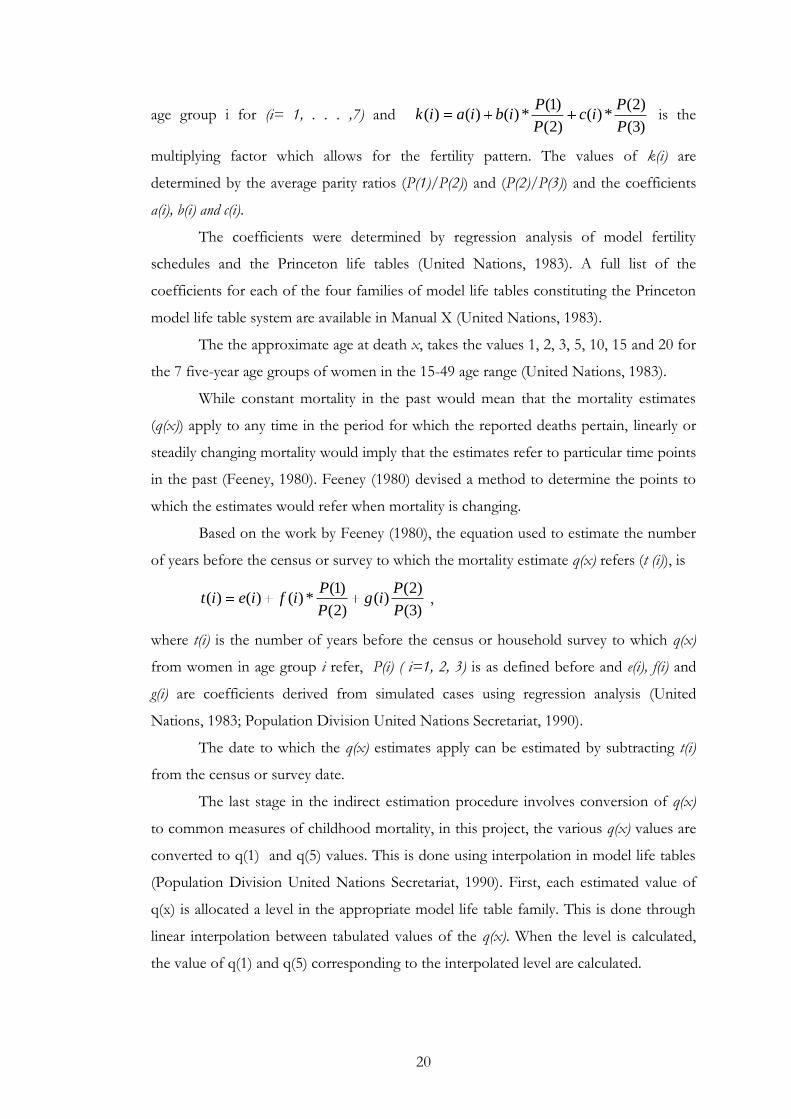
age x is )(*)()( iDikxq , where D(i) is the proportion of children dead for women in
20
age group i for (i= 1, . . . ,7) and )3(
)2(*)(
)2(
)1(*)()()(
P
Pic
P
Pibiaik is the
multiplying factor which allows for the fertility pattern. The values of k(i) are
determined by the average parity ratios (P(1)/P(2)) and (P(2)/P(3)) and the coefficients
a(i), b(i) and c(i).
The coefficients were determined by regression analysis of model fertility
schedules and the Princeton life tables (United Nations, 1983). A full list of the
coefficients for each of the four families of model life tables constituting the Princeton
model life table system are available in Manual X (United Nations, 1983).
The the approximate age at death x, takes the values 1, 2, 3, 5, 10, 15 and 20 for
the 7 five-year age groups of women in the 15-49 age range (United Nations, 1983).
While constant mortality in the past would mean that the mortality estimates
(q(x)) apply to any time in the period for which the reported deaths pertain, linearly or
steadily changing mortality would imply that the estimates refer to particular time points
in the past (Feeney, 1980). Feeney (1980) devised a method to determine the points to
which the estimates would refer when mortality is changing.
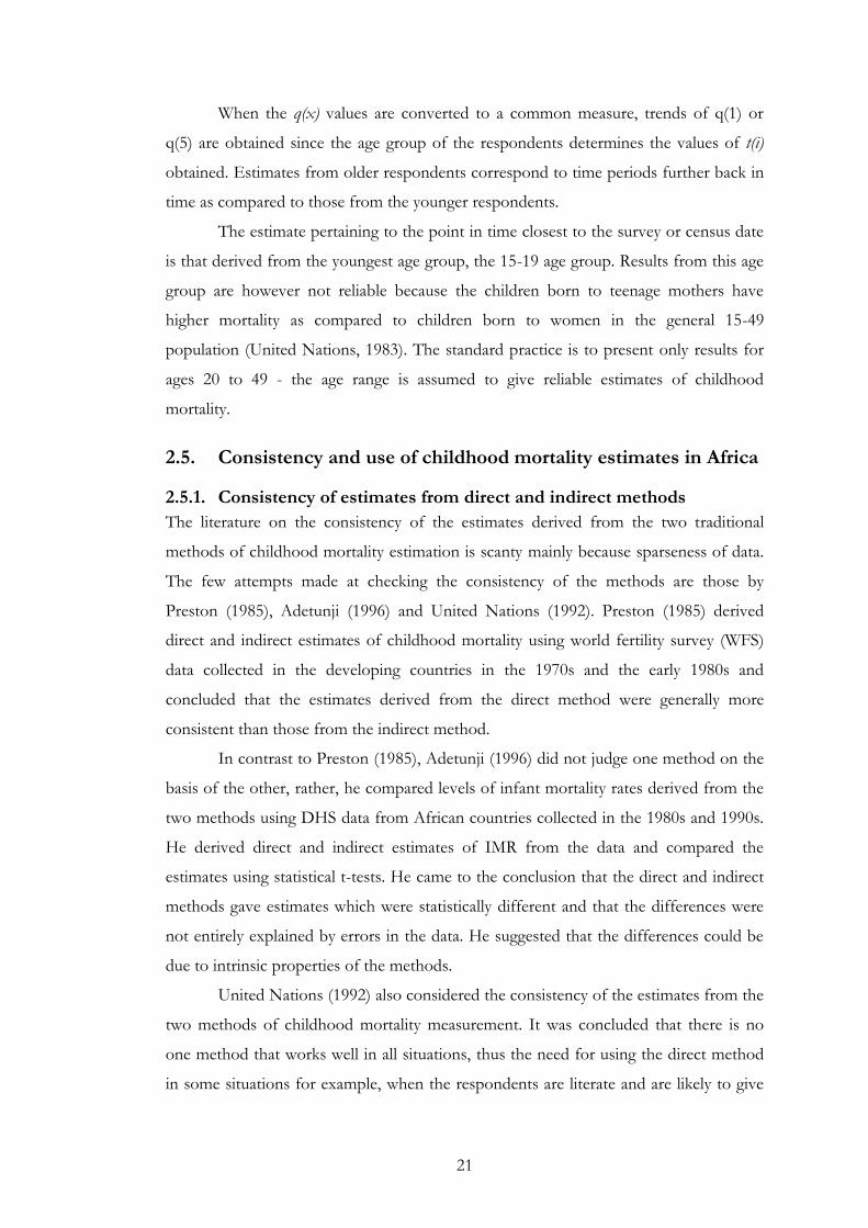
Based on the work by Feeney (1980), the equation used to estimate the number
of years before the census or survey to which the mortality estimate q(x) refers (t (i)), is
)3(
)2()(
)2(
)1(*)()()(
P
Pig
P
Pifieit ,
where t(i) is the number of years before the census or household survey to which q(x)
from women in age group i refer, P(i) ( i=1, 2, 3) is as defined before and e(i), f(i) and
g(i) are coefficients derived from simulated cases using regression analysis (United
Nations, 1983; Population Division United Nations Secretariat, 1990).
The date to which the q(x) estimates apply can be estimated by subtracting t(i)
from the census or survey date.
The last stage in the indirect estimation procedure involves conversion of q(x)
to common measures of childhood mortality, in this project, the various q(x) values are
converted to q(1) and q(5) values. This is done using interpolation in model life tables
(Population Division United Nations Secretariat, 1990). First, each estimated value of
q(x) is allocated a level in the appropriate model life table family. This is done through
linear interpolation between tabulated values of the q(x). When the level is calculated,
the value of q(1) and q(5) corresponding to the interpolated level are calculated.
21
When the q(x) values are converted to a common measure, trends of q(1) or
q(5) are obtained since the age group of the respondents determines the values of t(i)
obtained. Estimates from older respondents correspond to time periods further back in
time as compared to those from the younger respondents.
The estimate pertaining to the point in time closest to the survey or census date
is that derived from the youngest age group, the 15-19 age group. Results from this age
group are however not reliable because the children born to teenage mothers have
higher mortality as compared to children born to women in the general 15-49
population (United Nations, 1983). The standard practice is to present only results for
ages 20 to 49 - the age range is assumed to give reliable estimates of childhood
mortality.
2.5. Consistency and use of childhood mortality estimates in Africa
2.5.1. Consistency of estimates from direct and indirect methods
The literature on the consistency of the estimates derived from the two traditional
methods of childhood mortality estimation is scanty mainly because sparseness of data.
The few attempts made at checking the consistency of the methods are those by
Preston (1985), Adetunji (1996) and United Nations (1992). Preston (1985) derived
direct and indirect estimates of childhood mortality using world fertility survey (WFS)
data collected in the developing countries in the 1970s and the early 1980s and
concluded that the estimates derived from the direct method were generally more
consistent than those from the indirect method.
In contrast to Preston (1985), Adetunji (1996) did not judge one method on the
basis of the other, rather, he compared levels of infant mortality rates derived from the
two methods using DHS data from African countries collected in the 1980s and 1990s.
He derived direct and indirect estimates of IMR from the data and compared the
estimates using statistical t-tests. He came to the conclusion that the direct and indirect
methods gave estimates which were statistically different and that the differences were
not entirely explained by errors in the data. He suggested that the differences could be
due to intrinsic properties of the methods.
United Nations (1992) also considered the consistency of the estimates from the
two methods of childhood mortality measurement. It was concluded that there is no
one method that works well in all situations, thus the need for using the direct method
in some situations for example, when the respondents are literate and are likely to give
22
accurate dates of vital events and to use the indirect method in situations where the
available data for childhood mortality estimation are limited to just totals of children
ever born and children surviving.
2.5.2. Use of the estimates from the direct and the indirect methods
The two traditional methods of childhood mortality measurement have been used for
estimating levels and trends of childhood mortality in Africa (United Nations, 1992;
Hill, Pande and Mahy, 1999; Ahmad, Lopez and Inoue, 2000; Rutstein, 2000; Garenne
and Gakusi, 2006; Hill and Amouzou, 2006).
2.5.2.1. Trends in childhood mortality
The construction of the trends of childhood mortality has mainly focused on deriving a
consistent series from direct and indirect estimates. This is especially true in the work by
Hill and colleagues (United Nations, 1992; Hill, Pande and Mahy, 1999; Hill and
Amouzou, 2006). Combining direct and indirect estimates in a single series requires
understanding of the differences that exist between the estimates.
Other studies have relied more on the direct estimates derived from DHS data
than on the indirect estimates derived from censuses or other general national surveys
for construction of childhood mortality trends in Africa, only resorting to indirect
estimates in times of need. i.e., when direct estimates were unavailable (Ahmad, Lopez
and Inoue, 2000; Rutstein, 2000; Garenne and Gakusi, 2006).
The trends of childhood mortality in Africa constructed in the work just
mentioned above show that it has been improving since the beginning of the second
half of the twentieth century (Hill and Amouzou, 2006). The decline has mainly been
attributed to improvements in health and health interventions in the form of expanding
coverage of immunization programmes, prevention of malaria and provision of oral
rehydration solutions to children suffering from diarrhoea (Ahmad, Lopez and Inoue,
2000).
The decline in childhood mortality was most rapid from the early 1970s up to
the mid 1980s (Garenne and Gakusi, 2006; Hill and Amouzou, 2006). The period from
the late 1980s onwards, however, saw the childhood mortality decline slowing down,
worse still; stalling or even increasing in some African countries (Ahmad, Lopez and
Inoue, 2000). These adverse trends of childhood mortality coincided with the advent of
the HIV/AIDS epidemic among other negative conditions which included political
instability, and economic downturns (Adetunji, 2000; Ahmad, Lopez and Inoue, 2000;
23
Garenne and Gakusi, 2006; Hill and Amouzou, 2006). HIV was assumed to be the main
determinant of the worsening childhood mortality conditions.
The adverse childhood mortality conditions prevailing in most African countries
from the mid 1980s fostered the need for research to determine the causal role of HIV
in the levels and trends of childhood mortality (Walker, Schwartlander and Bryce, 2002).
However, the traditional methods of childhood mortality measurement were found to
be limited in their ability to answer questions on the exact role that HIV played in the
overall trends of childhood mortality. This was due to the potential biases in the data
and the unavailability prerequisite data for HIV impact assessment in Africa (Walker,
Schwartlander and Bryce, 2002; Zaba, Marston and Floyd, 2003).
2.6. Problems with the traditional methods of childhood mortality measurement in high HIV prevalence settings prevailing in African countries
There are two major problems which are related to the use of the traditional childhood
mortality estimation methods in high HIV prevalence settings. The first problem is the
violation of some of the assumptions required in the application of these methods
(Ward and Zaba, 1999; Mahy, 2003; Zaba, Marston and Floyd, 2003). The second
problem, which surfaces when wanting to attribute cause to mortality, is the lack of
national cause-specific childhood mortality data (Walker, Schwartlander and Bryce,
2002; Zaba, Marston and Floyd, 2003).
2.6.1. The violation of assumptions
The assumption that maternal and child mortality are independent is violated in high
HIV prevalence settings. This assumption is violated because of mother-to-child
transmission (vertical transmission) and the elevated mortality that results from HIV
infection (Ward and Zaba, 1999). The infected women are more likely to die than the
uninfected women in the period between giving birth and the survey or census. This
leads to the under-representation of the children of the infected women in the survey.
When the children of the infected women are under-represented, childhood mortality
will be under-estimated since these children experience higher mortality than the
children of the uninfected mothers, particularly since a proportion of them will be
infected with HIV (Berhane, Begenda, Marum et al., 1997; Brahmbhatt, Kigozi,
Wabwire-Mangen et al., 2006).
24
The assumption that the mortality of the children in the population of interest is
similar to the mortality described by a model life table no longer holds since the model
life tables mainly used (the Princeton or United Nations model life tables) were
constructed without taking HIV/AIDS into account so they do not capture the
additional deaths attributable to HIV/AIDS (Ward and Zaba, 1999; Mahy, 2003). The
other assumption violated is that of independence between childhood mortality and
maternal age. This is due to the fact that transmission of HIV from mother to child is
age dependent. (Ward and Zaba, 1999; Walker, Stanecki, Brown et al., 2003).
HIV also introduces errors in the time location of estimates. The coefficients
used in estimating the time location estimates were estimated from model life tables that
were constructed from HIV free data.
2.6.2. The absence of national cause-specific childhood mortality data
The evidence that AIDS is an important cause of childhood mortality is widely
acknowledged (Adetunji, 2000; Crampin, Floyd, Glynn et al., 2003; Nakiyingi, Bracher,
Whitworth et al., 2003; Ngweshemi, Urassa, Usingo et al., 2003; Hill, Cheluget, Curtis et
al., 2004). However, the understanding of the exact contribution of HIV/AIDS to the
overall level of childhood mortality is what remains limited. The contribution of
HIV/AIDS is not clearly understood because the nationally representative data used for
childhood mortality measurement in Africa are not cause of death specific. This makes
it difficult to estimate the contribution of HIV/AIDS to overall childhood mortality.
2.7. Understanding the effect of HIV on childhood mortality
Methods which are robust to the violation of the assumptions highlighted in the
previous section are required for accurate childhood mortality estimation in high HIV
prevalence settings. However, it is not enough to have only methods which provide
accurate overall childhood mortality estimates since observing overall mortality only
cannot give a good picture of the impact of HIV on childhood mortality. The
background mortality (mortality due to causes other than HIV/AIDS) may exaggerate
or mask the impact of HIV (Zaba, Marston and Floyd, 2003). This happens since it is
possible, depending on the level of prevalence, for overall mortality to keep declining
due to reduction in non-AIDS mortality while HIV related deaths are stable or even
increasing. There is therefore need to stratify childhood mortality by the HIV status of
the child.
25
The need for understanding the effect of HIV on childhood mortality in high
HIV prevalence settings has led to efforts being made towards verifying HIV
prevalence as a covariate of childhood mortality (Adetunji, 2000; Hill, Cheluget, Curtis
et al., 2004), development of new approaches to measurement of childhood mortality
and quantification of the impact of HIV on childhood mortality.
2.7.1. HIV prevalence as a covariate of childhood mortality
HIV prevalence has been included in regression relationships together with other
potential covariates of childhood mortality (Adetunji, 2000; Hill, Cheluget, Curtis et al.,
2004) to check it as a covariate. Adetunji (2000) concluded that HIV was an important,
but not the sole, cause of the adverse trends in childhood mortality in African countries.
Hill, Cheluget, Curtis et al (2004), in the study they did to check whether there was any
relationship between the reversal of the downward trends in childhood mortality in
Kenya and the increases in HIV prevalence in the same country, found that HIV
prevalence level was a significant covariate of childhood mortality in Kenya.
The results of longitudinal studies involving maternal HIV testing and child
survival in Africa have been summarized well by Newell, Brahmbhatt and Ghys (2004)
and Zaba (2003). These have indicated that the children of the HIV infected mothers
have higher mortality than the children of the uninfected mothers. Some longitudinal
studies have even gone further to stratify childhood mortality by both maternal and
child HIV status (Berhane, Begenda, Marum et al., 1997; Spira, Lepage, Msellati et al.,
1999; Taha, Kumwenda, Broadhead et al., 1999; Newell, Coovadia, Borja et al., 2004;
Brahmbhatt, Kigozi, Wabwire-Mangen et al., 2006; Marinda, Humphrey, Iliff et al.,
2007). The results from these studies indicated that the HIV infected children have the
highest mortality of all children, followed by the uninfected children of the HIV
infected mothers (the HIV exposed children). The children of the uninfected mothers
have generally been shown to have the lowest mortality of the three groups of children.
It has been concluded that HIV is indeed a covariate of childhood mortality.
Beyond establishing that HIV prevalence is a covariate, work has been done to
measure the extent to which it impacts childhood mortality. This has been done by
estimating the proportion of childhood mortality attributable to HIV/AIDS.
2.7.2. Proportion of childhood mortality attributable to HIV/AIDS
The effect of HIV on childhood mortality has been quantified using the population
attributable fraction of childhood mortality (HIV PAF).
26
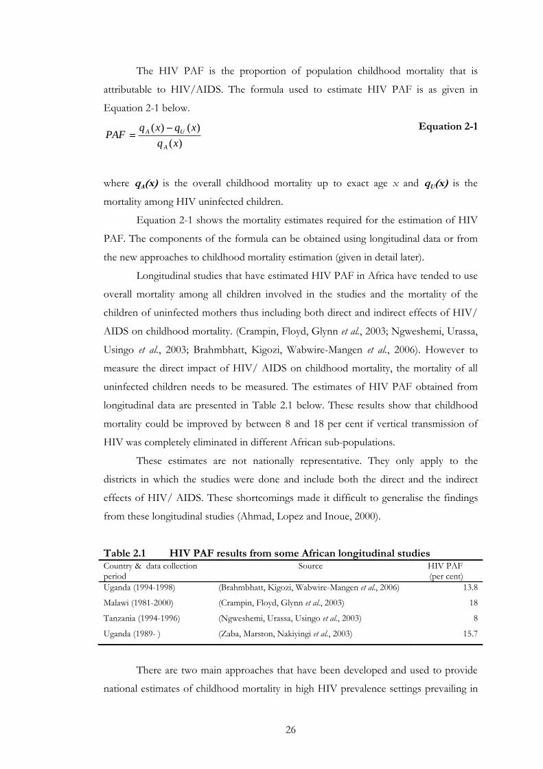
The HIV PAF is the proportion of population childhood mortality that is
attributable to HIV/AIDS. The formula used to estimate HIV PAF is as given in
Equation 2-1 below.
)(
)()(
xq
xqxqPAF
A
UA Equation 2-1
where qA(x) is the overall childhood mortality up to exact age x and qU(x) is the
mortality among HIV uninfected children.
Equation 2-1 shows the mortality estimates required for the estimation of HIV
PAF. The components of the formula can be obtained using longitudinal data or from
the new approaches to childhood mortality estimation (given in detail later).
Longitudinal studies that have estimated HIV PAF in Africa have tended to use
overall mortality among all children involved in the studies and the mortality of the
children of uninfected mothers thus including both direct and indirect effects of HIV/
AIDS on childhood mortality. (Crampin, Floyd, Glynn et al., 2003; Ngweshemi, Urassa,
Usingo et al., 2003; Brahmbhatt, Kigozi, Wabwire-Mangen et al., 2006). However to
measure the direct impact of HIV/ AIDS on childhood mortality, the mortality of all
uninfected children needs to be measured. The estimates of HIV PAF obtained from
longitudinal data are presented in Table 2.1 below. These results show that childhood
mortality could be improved by between 8 and 18 per cent if vertical transmission of
HIV was completely eliminated in different African sub-populations.
These estimates are not nationally representative. They only apply to the
districts in which the studies were done and include both the direct and the indirect
effects of HIV/ AIDS. These shortcomings made it difficult to generalise the findings
from these longitudinal studies (Ahmad, Lopez and Inoue, 2000).
Table 2.1 HIV PAF results from some African longitudinal studies Country & data collection period
Source HIV PAF (per cent)
Uganda (1994-1998) (Brahmbhatt, Kigozi, Wabwire-Mangen et al., 2006) 13.8
Malawi (1981-2000) (Crampin, Floyd, Glynn et al., 2003) 18
Tanzania (1994-1996) (Ngweshemi, Urassa, Usingo et al., 2003) 8
Uganda (1989- ) (Zaba, Marston, Nakiyingi et al., 2003) 15.7
There are two main approaches that have been developed and used to provide
national estimates of childhood mortality in high HIV prevalence settings prevailing in
27
most African countries. The childhood mortality estimates obtained from these
methods have been used to derive national estimates of HIV PAF. These two
approaches are described in detail in the next section.
2.8. New approaches to childhood mortality measurement
The approaches described below are termed “new” because they were devised to
estimate childhood mortality in the presence of HIV/ AIDS. They used not to exist in
the pre-AIDS era.
The two new approaches that have been mainly used to derive national
estimates of childhood mortality stratified by child HIV status in sub-Saharan Africa are
the method by Walker, Schwartlander and Bryce (2002) and the method by Zaba,
Marston and Floyd (2003), hereafter referred to in short as the Walker method and the
Zaba method respectively.
2.8.1. Walker method
Walker, Schwartlander and Bryce (2002) developed a method of measuring childhood
mortality in high HIV prevalence settings (high HIV settings defined in Chapter 1)
In this method, a four-step process is used to produce estimates of the age
specific mortality of HIV infected children and the proportion of all under-five deaths
that are attributable to HIV/AIDS. The steps are described in detail below
2.8.1.1. Estimation of prevalence among females of reproductive age
The Walker method starts with HIV prevalence among women attending antenatal
clinics at selected HIV prevalence sentinel surveillance sites. The point estimates of
HIV prevalence from sentinel surveillance sites are entered into a epidemiological
computer program developed by WHO called EPIMODEL (Schwartlander, Stanecki,
Brown et al., 1999) which implements a UNAIDS-developed HIV prevalence projection
model. This prevalence projection model fits HIV/AIDS epidemic curves to point
prevalence estimates. Details of how the model is fitted are given by Schwartlander,
Stanecki, Brown et al. (1999).
2.8.1.2. Estimation of the numbers of infected and uninfected children
The prevalence rates for adults aged 15 - 49 are applied to the reproductive female
population to get numbers of infected and uninfected women.
28
Appropriate fertility schedules from age specific fertility rates estimated by the
United Nations Population Division, are then applied to the resulting estimated
distributions of infected and uninfected women taking into account the effect of HIV
on fertility. Fertility of infected women 20 years or older, is assumed to be 20 per cent
lower than the fertility of the women of the same age in the national reproductive
female population. The fertility of infected pregnant teenagers (15-19) is assumed to be
50 per cent higher compared to the 15-19 women in the general population. The
teenage women who fall pregnant are assumed to be more sexually active and to be
more exposed to unprotected sex than women in the general population (Walker,
Stanecki, Brown et al., 2003; Zaba, Whiteside and Boerma, 2004).
Vertical transmission rates are applied to the births from HIV positive women
to estimate the proportion of births that gets infected. Account is taken of when the
vertical transmission occurred since vertical transmission rates are known to vary
depending on child’s age at infection (De Cock, Fowler, Mercier et al., 2000). The time
periods at which vertical transmission occurs are: in utero or intrapartum, in the first 6
months after birth or after the first six months. The variation in the transmission rates is
accounted for by grouping infected children into three cohorts depending on the timing
of infection. The transmission rates are estimated as ranges for each of the three periods
using results from work by De Cock, Fowler, Mercier et al (2000). The estimates of
vertical transmission used are 15-30 per cent for children getting infected in utero or at
birth (no transmission through breast milk), 25-35 per cent for children getting infected
in the first six months after birth through early breastfeeding and 30-45 per cent for
children getting infected after the first six months of life by late breastfeeding.
2.8.1.3. Survival from infection to death
Net survival of infected children from HIV/AIDS only in the time from infection to
death is modeled by a double Weibull distribution on the basis of results from African
studies involving vertical HIV transmission and survival (Walker, Schwartlander and
Bryce, 2002).
Survival of children after infection is assumed to be either long or short term.
Combinations of minimum and maximum transmission rates and long and short
survival periods give four scenarios. The four scenarios are; minimum transmission -
long survival, minimum transmission-short survival, maximum transmission-long
survival and maximum transmission-short survival. Four estimates of mortality are
29
obtained for each year and each of the countries being considered. The mean value of
the four estimates is used as the best estimate.
The results obtained are the numbers of children who die with the HIV
infection.
2.8.1.4. Number of children dying of HIV/AIDS
To obtain the number of childhood deaths directly attributable to HIV/AIDS, the
following steps are followed. First, the proportion of all childhood deaths due to causes
other than HIV/AIDS is estimated by subtracting the number of deaths among
infected children from the WHO all causes deaths and then dividing the difference by
the WHO number of deaths from all causes. Second, this proportion is multiplied by
the number of deaths among HIV infected children. The result is the number of HIV
infected children who die of non-AIDS causes. Third, the number of the HIV positive
children who die of causes other than AIDS is subtracted from the number of all the
HIV infected children dying to obtain childhood deaths directly resulting from
HIV/AIDS related causes.
After obtaining the estimated number of children dying of HIV/AIDS related
causes, the proportion of all deaths that is directly attributable to HIV/AIDS is
obtained by dividing the number of children dying of HIV/AIDS by the number of
childhood deaths from all causes.
2.8.2. The Zaba method
2.8.2.1. Mortality of the uninfected children
The starting point for the Zaba method is childhood mortality corresponding to the
period before the HIV/AIDS epidemic. Two time points, 10 years apart, are selected.
Both points are required to be either in the pre- HIV/AIDS epidemic period or the
later time point could be in the early years of the epidemic.
Since the logit transformations of mortality rates are linearly related (Zaba,
Marston and Floyd, 2003), Brass parameters relating the logit transformations of infant
and under-five mortality at the two chosen points are determined using an appropriate
standard, say a UN model life table (Zaba, Marston and Floyd, 2003). The linear change
in the parameters is extrapolated to an arbitrary point t in the future. The projected
parameters are used in the relational logit model of mortality to estimate infant and
under-five mortality. The equations explaining the extrapolation of the parameters are
outlined in Zaba, Marston and Floyd (2003).
30
2.8.2.2. Gross mortality of the HIV infected children
The next estimate to be derived is the mortality of infected children from HIV/AIDS
and non-HIV/AIDS causes, also called (by Zaba and colleagues) the gross mortality.
This is done by assuming independence between HIV/AIDS related causes and non-
HIV related causes and then using multiple decrement relationships. To derive the
cumulative probability of surviving from birth to age x for infected children (lI(x)), the
net survival from HIV/AIDS only (lN(x)) and the survival probability of the uninfected
children (lU(x)) are multiplied. The complement of lI(x) gives the gross mortality of
infected children.
Since the net mortality due to HIV/AIDS related causes only is unobservable, it
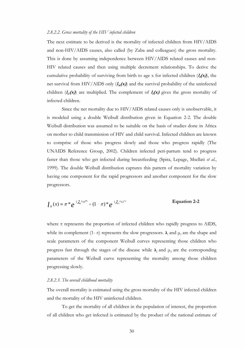
is modeled using a double Weibull distribution given in Equation 2-2. The double
Weibull distribution was assumed to be suitable on the basis of studies done in Africa
on mother to child transmission of HIV and child survival. Infected children are known
to comprise of those who progress slowly and those who progress rapidly (The
UNAIDS Reference Group, 2002). Children infected peri-partum tend to progress
faster than those who get infected during breastfeeding (Spira, Lepage, Msellati et al.,
1999). The double Weibull distribution captures this pattern of mortality variation by
having one component for the rapid progressors and another component for the slow
progressors.
eelxx
Nx
22
11
)*()*(*)1(*)(
Equation 2-2
where π represents the proportion of infected children who rapidly progress to AIDS,
while its complement (1- π) represents the slow progressors. 1 and μ1 are the shape and
scale parameters of the component Weibull curves representing those children who
progress fast through the stages of the disease while 2 and μ2 are the corresponding
parameters of the Weibull curve representing the mortality among those children
progressing slowly.
2.8.2.3. The overall childhood mortality
The overall mortality is estimated using the gross mortality of the HIV infected children
and the mortality of the HIV uninfected children.
To get the mortality of all children in the population of interest, the proportion
of all children who get infected is estimated by the product of the national estimate of
31
the HIV prevalence among pregnant women attending antenatal clinics (p) and the
mother to child transmission rate of HIV (v). The prevalence used in this methodology
was that recorded in sentinel surveillance sites and the mother to child transmission rate
used is 35 per cent which is the mid-point of the range of vertical transmission in
breastfeeding populations given in De Cock, Fowler, Mercier et al (2000). When this
method was developed, prevention of mother-to-child transmission of HIV was only
beginning to be implemented in most African countries so it was not considered in the
estimation of vertical transmission rate. The developers of the method however give
provision for adjusting the vertical transmission rate to accommodate PMTCT.
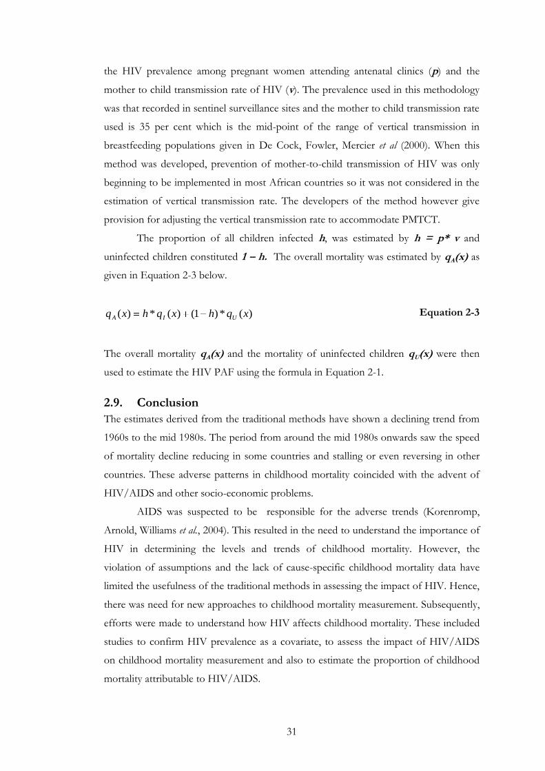
The proportion of all children infected h, was estimated by h = p* v and
uninfected children constituted 1 – h. The overall mortality was estimated by qA(x) as
given in Equation 2-3 below.
)(*)1()(*)( xqhxqhxq UIA Equation 2-3
The overall mortality qA(x) and the mortality of uninfected children qU(x) were then
used to estimate the HIV PAF using the formula in Equation 2-1.
2.9. Conclusion
The estimates derived from the traditional methods have shown a declining trend from
1960s to the mid 1980s. The period from around the mid 1980s onwards saw the speed
of mortality decline reducing in some countries and stalling or even reversing in other
countries. These adverse patterns in childhood mortality coincided with the advent of
HIV/AIDS and other socio-economic problems.
AIDS was suspected to be responsible for the adverse trends (Korenromp,
Arnold, Williams et al., 2004). This resulted in the need to understand the importance of
HIV in determining the levels and trends of childhood mortality. However, the
violation of assumptions and the lack of cause-specific childhood mortality data have
limited the usefulness of the traditional methods in assessing the impact of HIV. Hence,
there was need for new approaches to childhood mortality measurement. Subsequently,
efforts were made to understand how HIV affects childhood mortality. These included
studies to confirm HIV prevalence as a covariate, to assess the impact of HIV/AIDS
on childhood mortality measurement and also to estimate the proportion of childhood
mortality attributable to HIV/AIDS.
32
The studies that have investigated the relationship between HIV/AIDS and
childhood mortality in Africa have largely been longitudinal in nature. These studies
were mainly done in sub-populations of countries, usually single districts (Crampin,
Floyd, Glynn et al., 2003; Nakiyingi, Bracher, Whitworth et al., 2003; Ngweshemi,
Urassa, Usingo et al., 2003).
The mortality estimates derived from the data gathered in each of these
longitudinal studies were not nationally representative because of the spatial variation
of childhood mortality between regions within a country (Palamuleni, 2001; Zaba,
Marston and Floyd, 2003). Despite not being nationally representative, the data revealed
important characteristics of paediatric HIV infection and survival which have been used
to inform construction of models which are the current sources of national estimates of
the impact of HIV/AIDS on childhood mortality (The UNAIDS Reference Group,
2002; Walker, Schwartlander and Bryce, 2002; Zaba, Marston and Floyd, 2003; Johnson
and Dorrington, 2005).
Although models such as the Walker method are good at bridging the gap
between results from longitudinal studies and nationally representative estimates, they
have the weakness of being complex and less transparent (Zaba, Marston and Floyd,
2003).
Although a significant amount of work has been done to improve our
understanding of the way HIV affects childhood mortality and childhood mortality
measurement in Africa, there still remains unaddressed issues concerning the impact of
HIV on childhood mortality and childhood mortality measurement.
So far, trend analysis of childhood mortality has mainly focused on the
construction of a consistent series of estimates from the direct and the indirect
childhood mortality estimation methods. Little attention has been paid to the
comparison of trends from these two methods to verify whether the two methods
produce the same trend or not. It is important to verify whether the trends from the
two methods are consistent especially in high HIV prevalence settings since there are
suggestions that the indirect method is impacted more by HIV/AIDS than the direct
method (Mahy, 2003).
No study in Africa so far has used DHS birth histories data from HIV negative
women to derive childhood mortality estimates for uninfected children for use in
estimating HIV PAF. These birth histories could be a good basis for the estimation of
33
mortality of uninfected children for use in HIV PAF estimation (Zaba, Marston and
Floyd, 2003).
Chapter 4 addresses these two questions by providing a possible methodology
for comparison of the childhood mortality trends and assessing the impact of
HIV/AIDS on childhood mortality using DHS data involving HIV testing results and
results from African longitudinal data on vertical HIV transmission and child survival.
34
3. Data
3.1. Introduction
This chapter presents the sources of the data used in this project and an assessment of
their quality. Section 3.2 gives the background information on the two countries (Kenya
and Malawi) from which the data were collected. Section 3.3 gives the data sources.
Section 3.4 presents the assessment of data quality. Finally, section 3.5 gives the chapter
conclusion.
3.2. Background information on Kenya and Malawi
3.2.1. Kenya
Comprehensive background information about Kenya is provided in DHS survey
reports. The brief description of Kenya which follows has been mainly constructed
from the information in the 2003 Kenyan DHS report (Central Bureau of Statistics
(CBS) [Kenya], Ministry of Health (MOH) [Kenya] and ORC Macro, 2004).
Kenya is located in the eastern part of the African continent. It is bordered by
the United Republic of Tanzania to the south, Uganda to the west, Ethiopia and Sudan
to the north, Somalia to the north-east and the Indian Ocean to the south-east. The
total land area of Kenya is 582 646 square kilometres. 80 per cent of the land area is
either arid or semi arid. This non arable land is mainly used by nomadic pastoralists.
There are eight provinces in Kenya which are Central, Coast, Eastern, Nairobi,
North-Eastern, Nyanza, Rift Valley and Western provinces.
The last Kenyan census in 1999 reported the Kenyan population as 28.7 million
(Kenya National Bureau of Statistics, 2001). Projections reported by Population
Reference Bureau put the Kenyan population at 36.9million as of mid 2007 (Population
Reference Bureau, 2007) while the Kenyan Bureau of Statistics projected the population
to 37.2 million in August 2006 (National AIDS Control Council and Office of the
President Kenya, 2008).
3.2.2. Malawi
Malawi is a southern African country. It is bordered by the United Republic of Tanzania
to the north and northeast, by Mozambique to the east, south and southwest and to the
west and northwest by Zambia. The total area of Malawi is 118 484 square kilometers.
The country is divided into three regions namely the Northern, Central and the
35
Southern regions. Demographic data in Malawi have mainly been collected through
population censuses. The DHS surveys were started in 1992 (National Statistical Office
(NSO) [Malawi] and Macro International Inc, 1994; National Statistical Office (NSO)
[Malawi] and ORC Macro, 2005). The other data source is the 1996 Malawi knowledge,
Attitudes and Practices in Health survey. As enumerated in 1998, the Malawian
population was 9.9 million. the Malawian population was estimated as 13.1 for mid-
2007 by the Population reference bureau (Population Reference Bureau, 2007). The
National Statistical Office Malawi estimated population to be 13 187 632 by mid-2007
(National Statistical Office (NSO) [Malawi], 2008a). Childhood mortality in Malawi is
among the highest in the world (Kabudula, 2007). The infant mortality and under five
mortality reported by the National Statistical office for 2006 are 69 per thousand births
and 118 per thousand births respectively (National Statistical Office (NSO) [Malawi],
2008b)
3.3. Data sources
Most of the data used in this project are from Demographic and Health Surveys (DHS).
The DHS datasets used together with the periods of data collection are provided in
Table 3.1 below. In addition to the DHS data, census data were also used. The census
data used are from the Kenyan 1999 and the Malawian 1998 censuses. The reference
nights for these censuses are 24/25 August and 1/2 September respectively.
Table 3.1 DHS datasets and data collection periods Country Data collection period Mid-point of data
collection period
Reference date of
survey (in years)
Kenya 17 February to 15 August 1993
16 February to 29 July 1998
18 April to 15 September 2003
17 May
8 May
1 July
1993.4
1998.4
2003.5
Malawi 1 September to 10 November 1992
12 July to early November 2000
4 October 2004 to 31 January 2005
5 October
12 September
2 December 2004
1992.8
2000.7
2004.9
The reference dates of the DHS surveys in Table 3.1 above were obtained by expressing
the mid-points of the data collection periods (column 3) in years. These reference dates
were used (in Chapter 4) to estimate the mid-points of the five-year intervals by which
IMR and U5MR are presented in DHS reports.
36
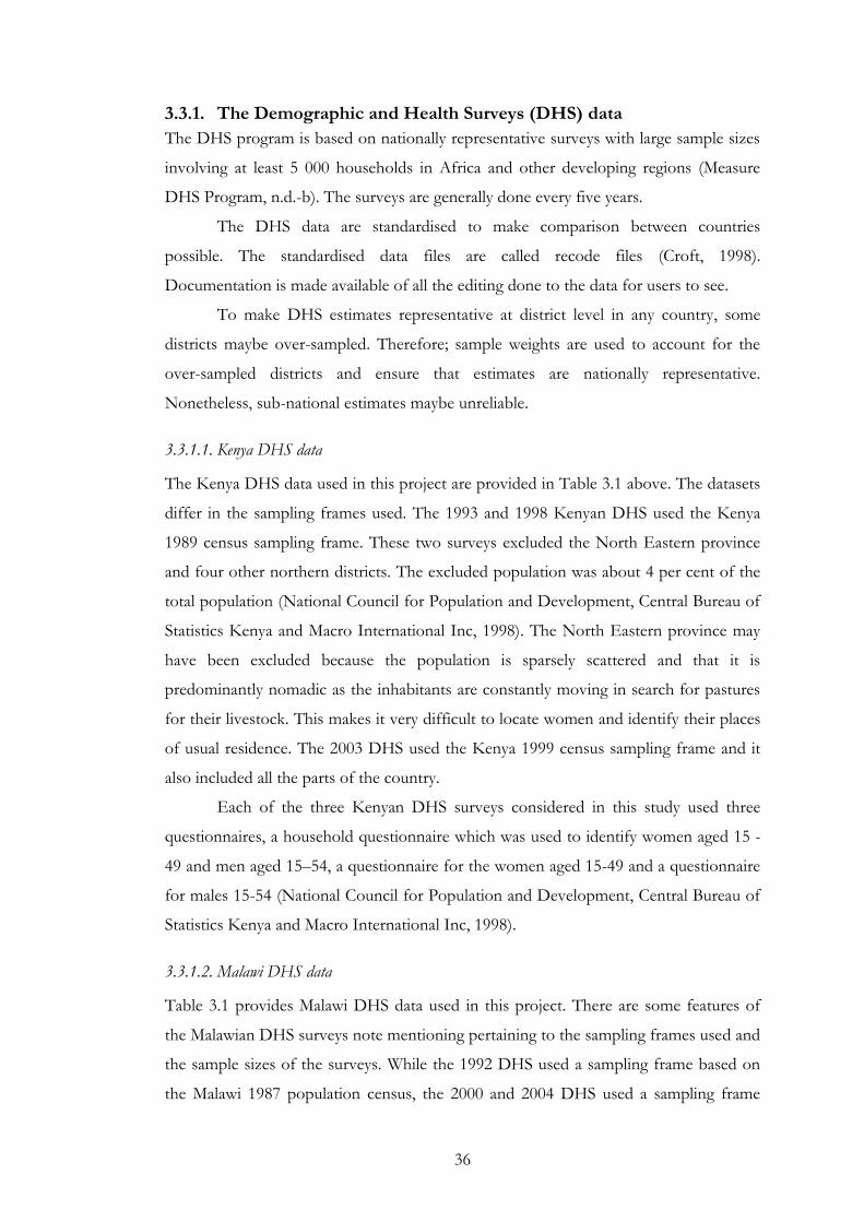
3.3.1. The Demographic and Health Surveys (DHS) data
The DHS program is based on nationally representative surveys with large sample sizes
involving at least 5 000 households in Africa and other developing regions (Measure
DHS Program, n.d.-b). The surveys are generally done every five years.
The DHS data are standardised to make comparison between countries
possible. The standardised data files are called recode files (Croft, 1998).
Documentation is made available of all the editing done to the data for users to see.
To make DHS estimates representative at district level in any country, some
districts maybe over-sampled. Therefore; sample weights are used to account for the
over-sampled districts and ensure that estimates are nationally representative.
Nonetheless, sub-national estimates maybe unreliable.
3.3.1.1. Kenya DHS data
The Kenya DHS data used in this project are provided in Table 3.1 above. The datasets
differ in the sampling frames used. The 1993 and 1998 Kenyan DHS used the Kenya
1989 census sampling frame. These two surveys excluded the North Eastern province
and four other northern districts. The excluded population was about 4 per cent of the
total population (National Council for Population and Development, Central Bureau of
Statistics Kenya and Macro International Inc, 1998). The North Eastern province may
have been excluded because the population is sparsely scattered and that it is
predominantly nomadic as the inhabitants are constantly moving in search for pastures
for their livestock. This makes it very difficult to locate women and identify their places
of usual residence. The 2003 DHS used the Kenya 1999 census sampling frame and it
also included all the parts of the country.
Each of the three Kenyan DHS surveys considered in this study used three
questionnaires, a household questionnaire which was used to identify women aged 15 -
49 and men aged 15–54, a questionnaire for the women aged 15-49 and a questionnaire
for males 15-54 (National Council for Population and Development, Central Bureau of
Statistics Kenya and Macro International Inc, 1998).
3.3.1.2. Malawi DHS data
Table 3.1 provides Malawi DHS data used in this project. There are some features of
the Malawian DHS surveys note mentioning pertaining to the sampling frames used and
the sample sizes of the surveys. While the 1992 DHS used a sampling frame based on
the Malawi 1987 population census, the 2000 and 2004 DHS used a sampling frame
37
based on the 1998 census. The 1992 sample of women of reproductive age was of size
4849. This sample was smaller than the later two DHS. The sample sizes for the 2000
and 2004 DHS were 13220 and 11698 respectively.
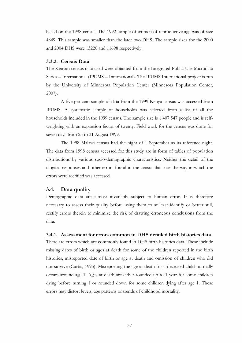
3.3.2. Census Data
The Kenyan census data used were obtained from the Integrated Public Use Microdata
Series – International (IPUMS – International). The IPUMS International project is run
by the University of Minnesota Population Center (Minnesota Population Center,
2007).
A five per cent sample of data from the 1999 Kenya census was accessed from
IPUMS. A systematic sample of households was selected from a list of all the
households included in the 1999 census. The sample size is 1 407 547 people and is self-
weighting with an expansion factor of twenty. Field work for the census was done for
seven days from 25 to 31 August 1999.
The 1998 Malawi census had the night of 1 September as its reference night.
The data from 1998 census accessed for this study are in form of tables of population
distributions by various socio-demographic characteristics. Neither the detail of the
illogical responses and other errors found in the census data nor the way in which the
errors were rectified was accessed.
3.4. Data quality
Demographic data are almost invariably subject to human error. It is therefore
necessary to assess their quality before using them to at least identify or better still,
rectify errors therein to minimize the risk of drawing erroneous conclusions from the
data.
3.4.1. Assessment for errors common in DHS detailed birth histories data
There are errors which are commonly found in DHS birth histories data. These include
missing dates of birth or ages at death for some of the children reported in the birth
histories, misreported date of birth or age at death and omission of children who did
not survive (Curtis, 1995). Misreporting the age at death for a deceased child normally
occurs around age 1. Ages at death are either rounded up to 1 year for some children
dying before turning 1 or rounded down for some children dying after age 1. These
errors may distort levels, age patterns or trends of childhood mortality.
38
Missing dates of birth or ages at death are imputed using a hot deck procedure
which involves identifying a child matching the child with missing information in other
variables and using the date of birth or age at death of this child (Curtis, 1995).
Assessment of DHS data for misreporting of ages at death and omission of
children who did not survive to survey dates is done for each DHS survey before
presenting the childhood mortality results.
Kenyan DHS reports for the three surveys used in this study show that there
was no significant misreporting of dates of births or dates of death or omission of dead
children in the surveys (National Council for Population and Development (NCPD),
central Bureau of Statistics (CBS) (Office of the Vice President and Planning and
Development [Kenya]) and Macro International Inc. (MI), 1994; National Council for
Population and Development, Central Bureau of Statistics Kenya and Macro
International Inc, 1998; Central Bureau of Statistics (CBS) [Kenya], Ministry of Health
(MOH) [Kenya] and ORC Macro, 2004).
Malawian 1992 and 2000 DHS reports did not indicate misreporting of dates of
births or ages at death in the birth histories. No omission of dead children was reported
for these two surveys (National Statistical Office (NSO) [Malawi] and Macro
International Inc, 1994; National Statistical Office (NSO) [Malawi] and ORC Macro,
2001).
The Malawi 2004 DHS report stated that there was misreporting of dates of
births. Births happening in the five-year period leading to the survey were reported to
have occurred in the earlier five-year period (National Statistical Office (NSO) [Malawi]
and ORC Macro, 2005). This transference of dates of births is said to be a result of
interviewers trying to reduce their workload by pushing dates of births backwards.
Pushing dates backwards eliminated the need to ask questions on child and maternal
health required for children born within the latest five year period prior to a DHS
survey. This transference of dates of births is said to lead to underestimation of
mortality in the five-year period immediately prior to the survey and overestimation in
the earlier five-year period.
Datasets were also assessed for general internal and external consistency by
assessing age distributions of the women aged 15-49, their educational characteristics,
parities and the interrelationships between these background characteristics. Anomalies
identified are mentioned.

39
It must however be noted that consistency does not imply the absence of errors
in the data. It is possible for datasets to pass consistency tests but nonetheless have
errors.
3.4.2. The quality of Kenyan data
Table 3.2 gives the basic demographic indicators for women aged 15-49 in the Kenyan
DHS surveys mentioned above and the 1999 Kenya census. Various background
characteristics of these women are investigated below to check the consistency of the
datasets used in this project.
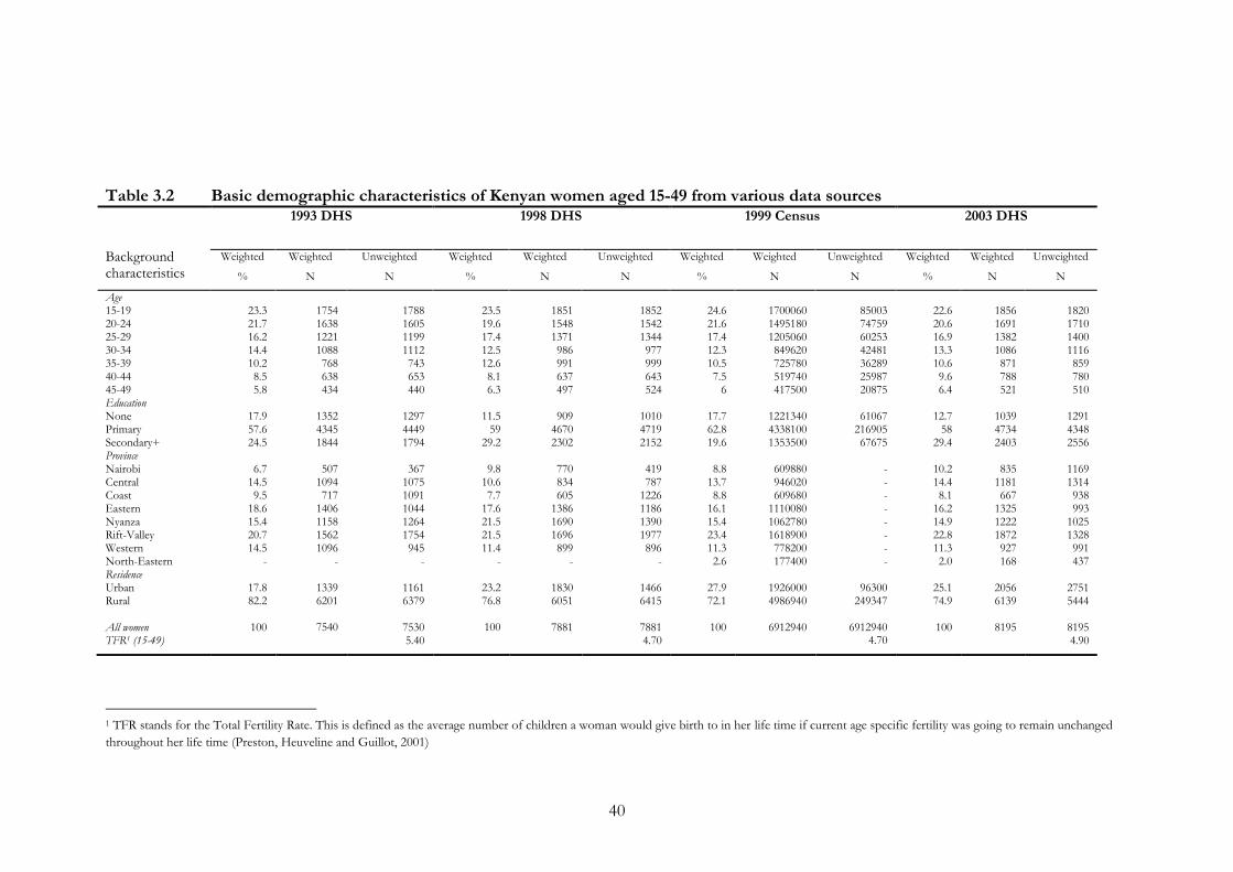
40
Table 3.2 Basic demographic characteristics of Kenyan women aged 15-49 from various data sources
Background characteristics
1993 DHS
1998 DHS 1999 Census 2003 DHS
Weighted
%
Weighted
N
Unweighted
N
Weighted
%
Weighted
N
Unweighted
N
Weighted
%
Weighted
N
Unweighted
N
Weighted
%
Weighted
N
Unweighted
N
Age 15-19 20-24 25-29 30-34 35-39 40-44 45-49 Education None Primary Secondary+ Province Nairobi Central Coast Eastern Nyanza Rift-Valley Western North-Eastern Residence Urban Rural All women TFR1 (15-49)
23.3 21.7 16.2 14.4 10.2 8.5 5.8
17.9 57.6 24.5
6.7
14.5 9.5
18.6 15.4 20.7 14.5
-
17.8 82.2
100
1754 1638 1221 1088 768 638 434
1352 4345 1844
507
1094 717
1406 1158 1562 1096
-
1339 6201
7540
1788 1605 1199 1112 743 653 440
1297 4449 1794
367
1075 1091 1044 1264 1754 945
-
1161 6379
7530 5.40
23.5 19.6 17.4 12.5 12.6 8.1 6.3
11.5
59 29.2
9.8
10.6 7.7
17.6 21.5 21.5 11.4
-
23.2 76.8
100
1851 1548 1371 986 991 637 497
909
4670 2302
770 834 605
1386 1690 1696 899
-
1830 6051
7881
1852 1542 1344 977 999 643 524
1010 4719 2152
419 787
1226 1186 1390 1977 896
-
1466 6415
7881 4.70
24.6 21.6 17.4 12.3 10.5 7.5
6
17.7 62.8 19.6
8.8 13.7 8.8
16.1 15.4 23.4 11.3 2.6
27.9 72.1
100
1700060 1495180 1205060 849620 725780 519740 417500
1221340 4338100 1353500
609880 946020 609680
1110080 1062780 1618900 778200 177400
1926000 4986940
6912940
85003 74759 60253 42481 36289 25987 20875
61067
216905 67675
- - - - - - - -
96300 249347
6912940
4.70
22.6 20.6 16.9 13.3 10.6 9.6 6.4
12.7
58 29.4
10.2 14.4 8.1
16.2 14.9 22.8 11.3 2.0
25.1 74.9
100
1856 1691 1382 1086 871 788 521
1039 4734 2403
835
1181 667
1325 1222 1872 927 168
2056 6139
8195
1820 1710 1400 1116 859 780 510
1291 4348 2556
1169 1314 938 993
1025 1328 991 437
2751 5444
8195 4.90
1 TFR stands for the Total Fertility Rate. This is defined as the average number of children a woman would give birth to in her life time if current age specific fertility was going to remain unchanged
throughout her life time (Preston, Heuveline and Guillot, 2001)
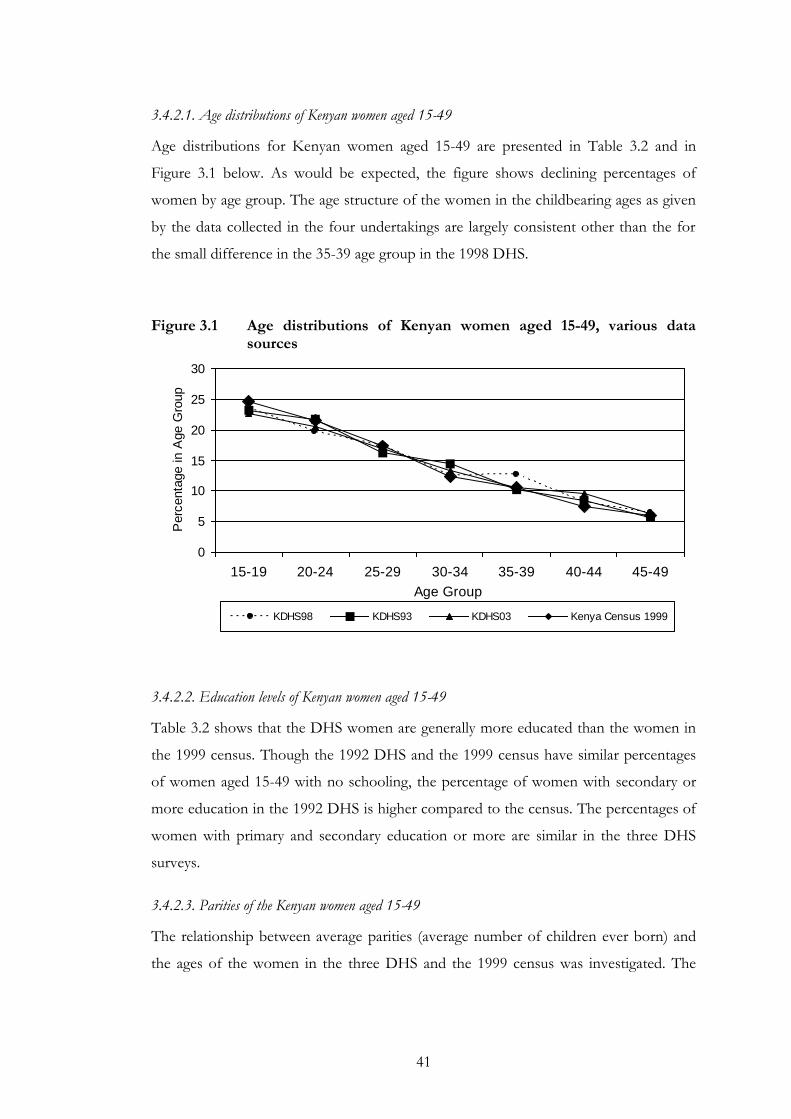
41
3.4.2.1. Age distributions of Kenyan women aged 15-49
Age distributions for Kenyan women aged 15-49 are presented in Table 3.2 and in
Figure 3.1 below. As would be expected, the figure shows declining percentages of
women by age group. The age structure of the women in the childbearing ages as given
by the data collected in the four undertakings are largely consistent other than the for
the small difference in the 35-39 age group in the 1998 DHS.
Figure 3.1 Age distributions of Kenyan women aged 15-49, various data
sources
0
5
10
15
20
25
30
15-19 20-24 25-29 30-34 35-39 40-44 45-49
Age Group
Perc
enta
ge in A
ge G
roup
KDHS98 KDHS93 KDHS03 Kenya Census 1999
3.4.2.2. Education levels of Kenyan women aged 15-49
Table 3.2 shows that the DHS women are generally more educated than the women in
the 1999 census. Though the 1992 DHS and the 1999 census have similar percentages
of women aged 15-49 with no schooling, the percentage of women with secondary or
more education in the 1992 DHS is higher compared to the census. The percentages of
women with primary and secondary education or more are similar in the three DHS
surveys.
3.4.2.3. Parities of the Kenyan women aged 15-49
The relationship between average parities (average number of children ever born) and
the ages of the women in the three DHS and the 1999 census was investigated. The
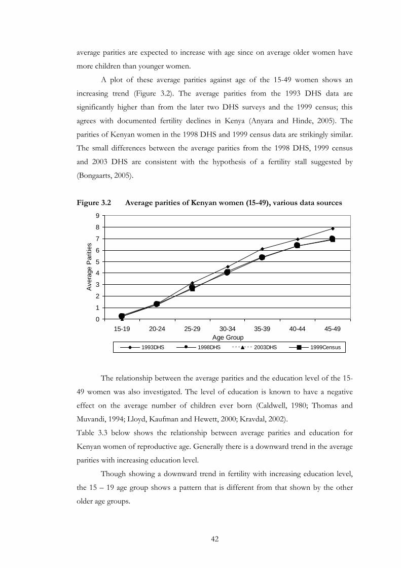
42
average parities are expected to increase with age since on average older women have
more children than younger women.
A plot of these average parities against age of the 15-49 women shows an
increasing trend (Figure 3.2). The average parities from the 1993 DHS data are
significantly higher than from the later two DHS surveys and the 1999 census; this
agrees with documented fertility declines in Kenya (Anyara and Hinde, 2005). The
parities of Kenyan women in the 1998 DHS and 1999 census data are strikingly similar.
The small differences between the average parities from the 1998 DHS, 1999 census
and 2003 DHS are consistent with the hypothesis of a fertility stall suggested by
(Bongaarts, 2005).
Figure 3.2 Average parities of Kenyan women (15-49), various data sources
0
1
2
3
4
5
6
7
8
9
15-19 20-24 25-29 30-34 35-39 40-44 45-49
Age Group
Avera
ge P
arities
1993DHS 1998DHS 2003DHS 1999Census
The relationship between the average parities and the education level of the 15-
49 women was also investigated. The level of education is known to have a negative
effect on the average number of children ever born (Caldwell, 1980; Thomas and
Muvandi, 1994; Lloyd, Kaufman and Hewett, 2000; Kravdal, 2002).
Table 3.3 below shows the relationship between average parities and education for
Kenyan women of reproductive age. Generally there is a downward trend in the average
parities with increasing education level.
Though showing a downward trend in fertility with increasing education level,
the 15 – 19 age group shows a pattern that is different from that shown by the other
older age groups.
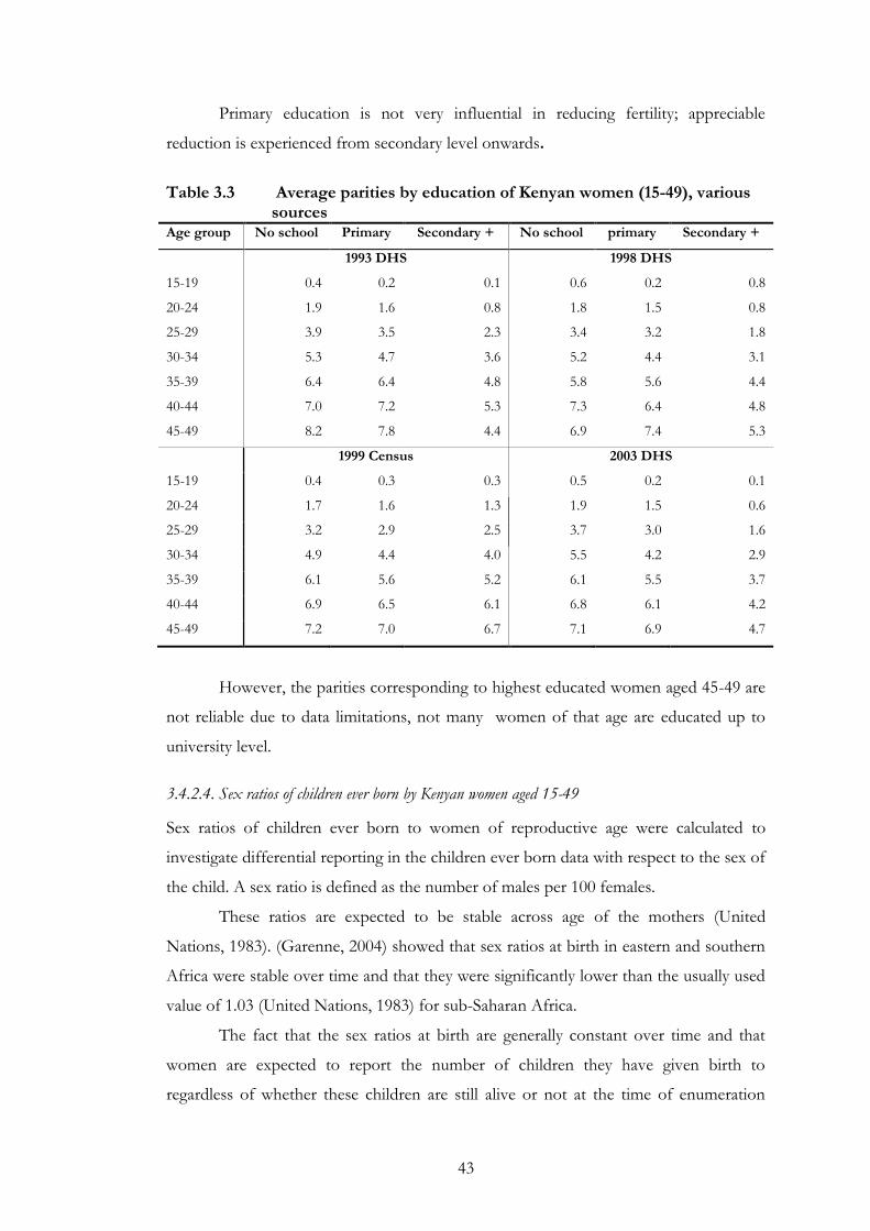
43
Primary education is not very influential in reducing fertility; appreciable
reduction is experienced from secondary level onwards.
Table 3.3 Average parities by education of Kenyan women (15-49), various
sources Age group No school Primary Secondary + No school primary Secondary +
1993 DHS 1998 DHS
15-19 0.4 0.2 0.1 0.6 0.2 0.8
20-24 1.9 1.6 0.8 1.8 1.5 0.8
25-29 3.9 3.5 2.3 3.4 3.2 1.8
30-34 5.3 4.7 3.6 5.2 4.4 3.1
35-39 6.4 6.4 4.8 5.8 5.6 4.4
40-44 7.0 7.2 5.3 7.3 6.4 4.8
45-49 8.2 7.8 4.4 6.9 7.4 5.3
1999 Census 2003 DHS
15-19 0.4 0.3 0.3 0.5 0.2 0.1
20-24 1.7 1.6 1.3 1.9 1.5 0.6
25-29 3.2 2.9 2.5 3.7 3.0 1.6
30-34 4.9 4.4 4.0 5.5 4.2 2.9
35-39 6.1 5.6 5.2 6.1 5.5 3.7
40-44 6.9 6.5 6.1 6.8 6.1 4.2
45-49 7.2 7.0 6.7 7.1 6.9 4.7
However, the parities corresponding to highest educated women aged 45-49 are
not reliable due to data limitations, not many women of that age are educated up to
university level.
3.4.2.4. Sex ratios of children ever born by Kenyan women aged 15-49
Sex ratios of children ever born to women of reproductive age were calculated to
investigate differential reporting in the children ever born data with respect to the sex of
the child. A sex ratio is defined as the number of males per 100 females.
These ratios are expected to be stable across age of the mothers (United
Nations, 1983). (Garenne, 2004) showed that sex ratios at birth in eastern and southern
Africa were stable over time and that they were significantly lower than the usually used
value of 1.03 (United Nations, 1983) for sub-Saharan Africa.
The fact that the sex ratios at birth are generally constant over time and that
women are expected to report the number of children they have given birth to
regardless of whether these children are still alive or not at the time of enumeration
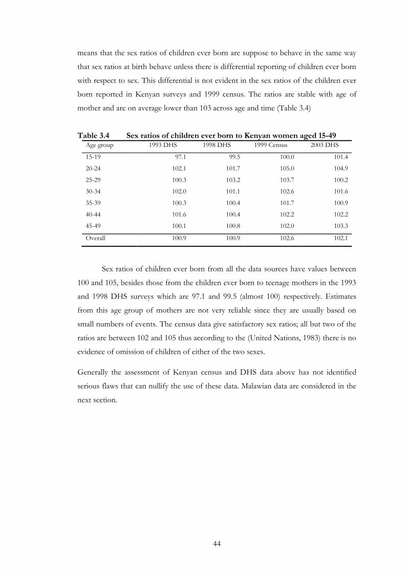
44
means that the sex ratios of children ever born are suppose to behave in the same way
that sex ratios at birth behave unless there is differential reporting of children ever born
with respect to sex. This differential is not evident in the sex ratios of the children ever
born reported in Kenyan surveys and 1999 census. The ratios are stable with age of
mother and are on average lower than 103 across age and time (Table 3.4)
Table 3.4 Sex ratios of children ever born to Kenyan women aged 15-49 Age group 1993 DHS 1998 DHS 1999 Census 2003 DHS
15-19 97.1 99.5 100.0 101.4
20-24 102.1 101.7 105.0 104.9
25-29 100.3 103.2 103.7 100.2
30-34 102.0 101.1 102.6 101.6
35-39 100.3 100.4 101.7 100.9
40-44 101.6 100.4 102.2 102.2
45-49 100.1 100.8 102.0 103.3
Overall 100.9 100.9 102.6 102.1
Sex ratios of children ever born from all the data sources have values between
100 and 105, besides those from the children ever born to teenage mothers in the 1993
and 1998 DHS surveys which are 97.1 and 99.5 (almost 100) respectively. Estimates
from this age group of mothers are not very reliable since they are usually based on
small numbers of events. The census data give satisfactory sex ratios; all but two of the
ratios are between 102 and 105 thus according to the (United Nations, 1983) there is no
evidence of omission of children of either of the two sexes.
Generally the assessment of Kenyan census and DHS data above has not identified
serious flaws that can nullify the use of these data. Malawian data are considered in the
next section.
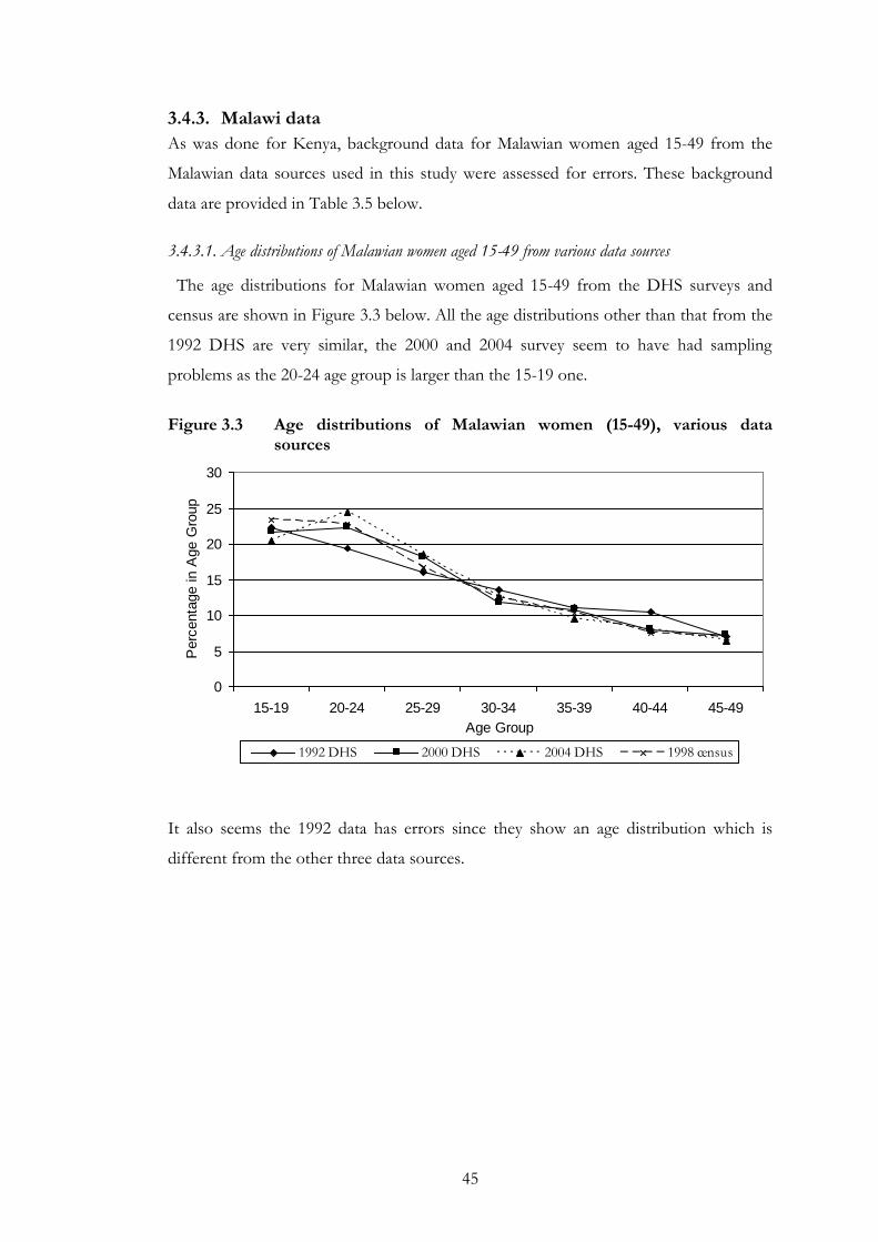
45
3.4.3. Malawi data
As was done for Kenya, background data for Malawian women aged 15-49 from the
Malawian data sources used in this study were assessed for errors. These background
data are provided in Table 3.5 below.
3.4.3.1. Age distributions of Malawian women aged 15-49 from various data sources
The age distributions for Malawian women aged 15-49 from the DHS surveys and
census are shown in Figure 3.3 below. All the age distributions other than that from the
1992 DHS are very similar, the 2000 and 2004 survey seem to have had sampling
problems as the 20-24 age group is larger than the 15-19 one.
Figure 3.3 Age distributions of Malawian women (15-49), various data
sources
0
5
10
15
20
25
30
15-19 20-24 25-29 30-34 35-39 40-44 45-49
Age Group
Perc
enta
ge in A
ge G
roup
1992 DHS 2000 DHS 2004 DHS 1998 census
It also seems the 1992 data has errors since they show an age distribution which is
different from the other three data sources.
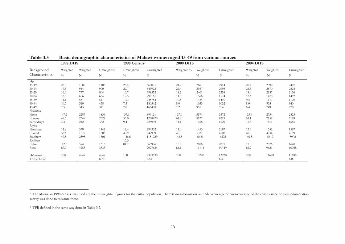
46
Table 3.5 Basic demographic characteristics of Malawi women aged 15-49 from various sources
Background Characteristics
1992 DHS 1998 Census2 2000 DHS 2004 DHS
Weighted
% Weighted
N Unweighted
N Unweighted
% Unweighted
N Weighted % Weighted
N Unweighted
N Weighted
% Weighted
N Unweighted
N
Age 15-19 20-24 25-29 30-34 35-39 40-44 45-49 Education None Primary Secondary+ Region Northern Central Southern Residence Urban Rural All women TFR (15-49)3
22.3 19.5 16.0 13.5 11.1 10.5 7.5 47.2 48.5 4.4 11.9 38.6 49.5 12.3 87.7 100
1082 944 777 656 537 510 343 2287 2349 212 578 1872 2398 594 4255 4849
1105 990 804 664 517 458 311 1834 2622 382 1442 1606 1801 1316 3533 4849 6.73
23.4 22.7 16.7 12.5 10.3 7.5 7.0 37.6 53.0 9.4 12.4 40.9
46.6 15.3 84.7 100
560071 543922 398552 298161 245784 180542 166498 899121 1268470 225939 294362 947939 1151229 365906 2027624 2393530 6.52
21.7 22.4 18.2 11.8 10.8 8.0 7.2 27.0 61.8 11.1 11.0 40.3 48.8 15.9 84.1 100
2867 2957 2401 1566 1424 1053 951 3574 8177 1468 1453 5321 6446 2106 11114 13220
2914 2998 2358 1574 1410 1052 914 3372 8219 1629 2187 4508 6525 2871 10349 13220 6.30
20.4 24.5 18.4 12.6 9.5 8.0 6.4 23.4 61.1 15.5 13.3 40.5 46.3 17.8 82.2 100
2392 2870 2157 1478 1117 935 749 2734 7152 1811 1552 4734 5412 2076 9621 11698
2407 2824 2136 1492 1129 940 770 2823 7189 1685 1597 4199 5902 1640 10058 11698 6.00
2 The Malawian 1998 census data used are the un-weighted figures for the entire population. There is no information on under-coverage or over-coverage of the census since no post-enumeration
survey was done to measure these.
3 TFR defined in the same way done in Table 3.2.
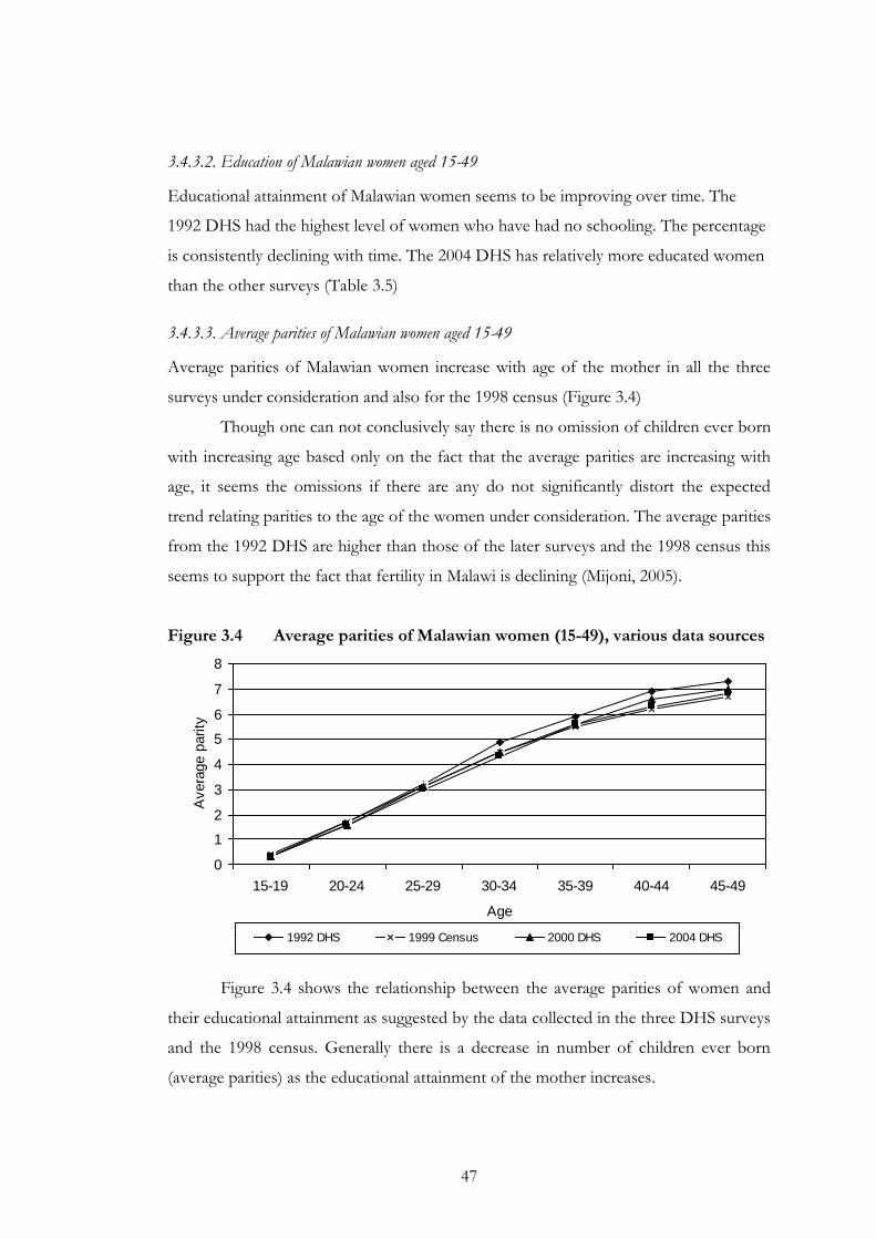
47
3.4.3.2. Education of Malawian women aged 15-49
Educational attainment of Malawian women seems to be improving over time. The
1992 DHS had the highest level of women who have had no schooling. The percentage
is consistently declining with time. The 2004 DHS has relatively more educated women
than the other surveys (Table 3.5)
3.4.3.3. Average parities of Malawian women aged 15-49
Average parities of Malawian women increase with age of the mother in all the three
surveys under consideration and also for the 1998 census (Figure 3.4)
Though one can not conclusively say there is no omission of children ever born
with increasing age based only on the fact that the average parities are increasing with
age, it seems the omissions if there are any do not significantly distort the expected
trend relating parities to the age of the women under consideration. The average parities
from the 1992 DHS are higher than those of the later surveys and the 1998 census this
seems to support the fact that fertility in Malawi is declining (Mijoni, 2005).
Figure 3.4 Average parities of Malawian women (15-49), various data sources
0
1
2
3
4
5
6
7
8
15-19 20-24 25-29 30-34 35-39 40-44 45-49
Age
Avera
ge p
arity
1992 DHS 1999 Census 2000 DHS 2004 DHS
Figure 3.4 shows the relationship between the average parities of women and
their educational attainment as suggested by the data collected in the three DHS surveys
and the 1998 census. Generally there is a decrease in number of children ever born
(average parities) as the educational attainment of the mother increases.
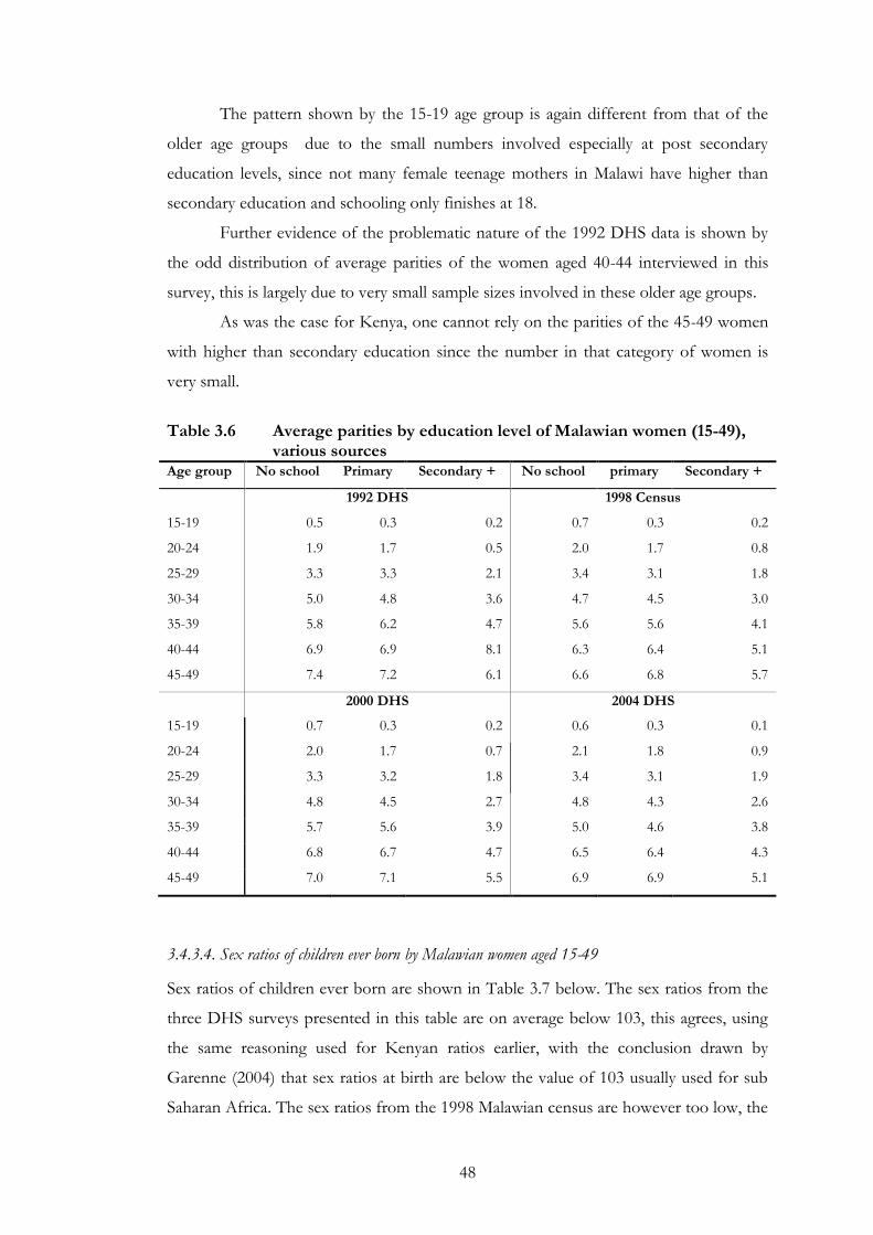
48
The pattern shown by the 15-19 age group is again different from that of the
older age groups due to the small numbers involved especially at post secondary
education levels, since not many female teenage mothers in Malawi have higher than
secondary education and schooling only finishes at 18.
Further evidence of the problematic nature of the 1992 DHS data is shown by
the odd distribution of average parities of the women aged 40-44 interviewed in this
survey, this is largely due to very small sample sizes involved in these older age groups.
As was the case for Kenya, one cannot rely on the parities of the 45-49 women
with higher than secondary education since the number in that category of women is
very small.
Table 3.6 Average parities by education level of Malawian women (15-49),
various sources Age group No school Primary Secondary + No school primary Secondary +
1992 DHS 1998 Census
15-19 0.5 0.3 0.2 0.7 0.3 0.2
20-24 1.9 1.7 0.5 2.0 1.7 0.8
25-29 3.3 3.3 2.1 3.4 3.1 1.8
30-34 5.0 4.8 3.6 4.7 4.5 3.0
35-39 5.8 6.2 4.7 5.6 5.6 4.1
40-44 6.9 6.9 8.1 6.3 6.4 5.1
45-49 7.4 7.2 6.1 6.6 6.8 5.7
2000 DHS 2004 DHS
15-19 0.7 0.3 0.2 0.6 0.3 0.1
20-24 2.0 1.7 0.7 2.1 1.8 0.9
25-29 3.3 3.2 1.8 3.4 3.1 1.9
30-34 4.8 4.5 2.7 4.8 4.3 2.6
35-39 5.7 5.6 3.9 5.0 4.6 3.8
40-44 6.8 6.7 4.7 6.5 6.4 4.3
45-49 7.0 7.1 5.5 6.9 6.9 5.1
3.4.3.4. Sex ratios of children ever born by Malawian women aged 15-49
Sex ratios of children ever born are shown in Table 3.7 below. The sex ratios from the
three DHS surveys presented in this table are on average below 103, this agrees, using
the same reasoning used for Kenyan ratios earlier, with the conclusion drawn by
Garenne (2004) that sex ratios at birth are below the value of 103 usually used for sub
Saharan Africa. The sex ratios from the 1998 Malawian census are however too low, the
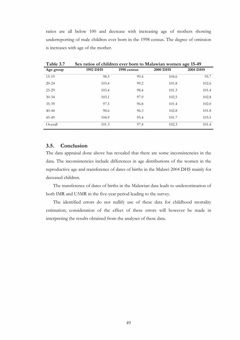
49
ratios are all below 100 and decrease with increasing age of mothers showing
underreporting of male children ever born in the 1998 census. The degree of omission
is increases with age of the mother.
Table 3.7 Sex ratios of children ever born to Malawian women age 15-49 Age group 1992 DHS 1998 census 2000 DHS 2004 DHS
15-19 98.3 99.4 104.6 95.7
20-24 103.4 99.2 101.8 102.6
25-29 103.4 98.4 101.3 101.4
30-34 103.1 97.9 102.5 102.8
35-39 97.5 96.8 101.4 102.0
40-44 98.6 96.3 102.8 101.8
45-49 104.9 95.4 101.7 103.5
Overall 101.3 97.4 102.3 101.4
3.5. Conclusion
The data appraisal done above has revealed that there are some inconsistencies in the
data. The inconsistencies include differences in age distributions of the women in the
reproductive age and transference of dates of births in the Malawi 2004 DHS mainly for
deceased children.
The transference of dates of births in the Malawian data leads to underestimation of
both IMR and U5MR in the five-year period leading to the survey.
The identified errors do not nullify use of these data for childhood mortality
estimation; consideration of the effect of these errors will however be made in
interpreting the results obtained from the analyses of these data.
50
4. Comparison of childhood mortality trends
4.1. Introduction
This chapter outlines the method used to compare the trends of childhood mortality
estimates from the direct and the indirect methods. It also presents the results obtained.
Section 4.2 gives the methods used to derive the direct and indirect estimates and the
resulting childhood mortality rates. Then section 4.3 compares the trends. The last
section (4.4) gives the conclusion.
4.2. Trends of direct and indirect estimates of childhood mortality
4.2.1. Direct childhood mortality estimates
An SPSS program used to derive childhood mortality rates presented in the DHS
reports (Measure DHS Program, n.d.-a) was converted into a STATA 9.2 program. The
STATA code (an illustration is provided in section 3A of the Appendix) was then
shown to produce the same estimates as those presented in the DHS reports for all the
DHS used at in this study. Table 4.1 and Table 4.2 provide the estimates as reported in
the DHS reports and those from the STATA code used for the current study. The
estimates derived from the STATA code are labelled as calculated while those from the
DHS reports are given as reported. The columns labelled Time refer to the mid-points of
the five-year periods before the survey to which the estimates pertain.
4.2.1.1. Derivation of the years to which direct estimates of childhood mortality refer
IMR and U5MR in DHS reports are provided by five year periods preceding the survey.
These intervals could not be used in comparing childhood mortality trends from the
direct and the indirect methods since the indirect estimates were tabulated by specific
years. Instead of the five-year intervals, the mid-points of these intervals were used.
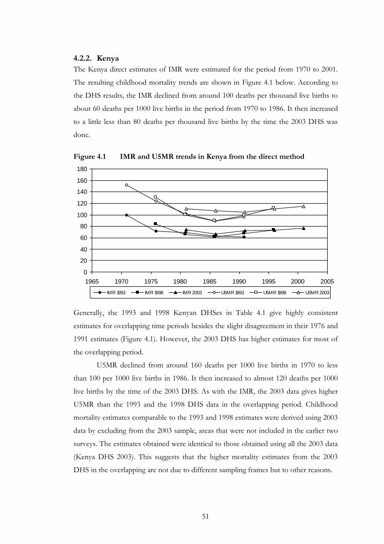
51
4.2.2. Kenya
The Kenya direct estimates of IMR were estimated for the period from 1970 to 2001.
The resulting childhood mortality trends are shown in Figure 4.1 below. According to
the DHS results, the IMR declined from around 100 deaths per thousand live births to
about 60 deaths per 1000 live births in the period from 1970 to 1986. It then increased
to a little less than 80 deaths per thousand live births by the time the 2003 DHS was
done.
Figure 4.1 IMR and U5MR trends in Kenya from the direct method
0
20
40
60
80
100
120
140
160
180
1965 1970 1975 1980 1985 1990 1995 2000 2005
IMR 1993 IMR 1998 IMR 2003 U5MR 1993 U5MR 1998 U5MR 2003
Generally, the 1993 and 1998 Kenyan DHSes in Table 4.1 give highly consistent
estimates for overlapping time periods besides the slight disagreement in their 1976 and
1991 estimates (Figure 4.1). However, the 2003 DHS has higher estimates for most of
the overlapping period.
U5MR declined from around 160 deaths per 1000 live births in 1970 to less
than 100 per 1000 live births in 1986. It then increased to almost 120 deaths per 1000
live births by the time of the 2003 DHS. As with the IMR, the 2003 data gives higher
U5MR than the 1993 and the 1998 DHS data in the overlapping period. Childhood
mortality estimates comparable to the 1993 and 1998 estimates were derived using 2003
data by excluding from the 2003 sample, areas that were not included in the earlier two
surveys. The estimates obtained were identical to those obtained using all the 2003 data
(Kenya DHS 2003). This suggests that the higher mortality estimates from the 2003
DHS in the overlapping are not due to different sampling frames but to other reasons.
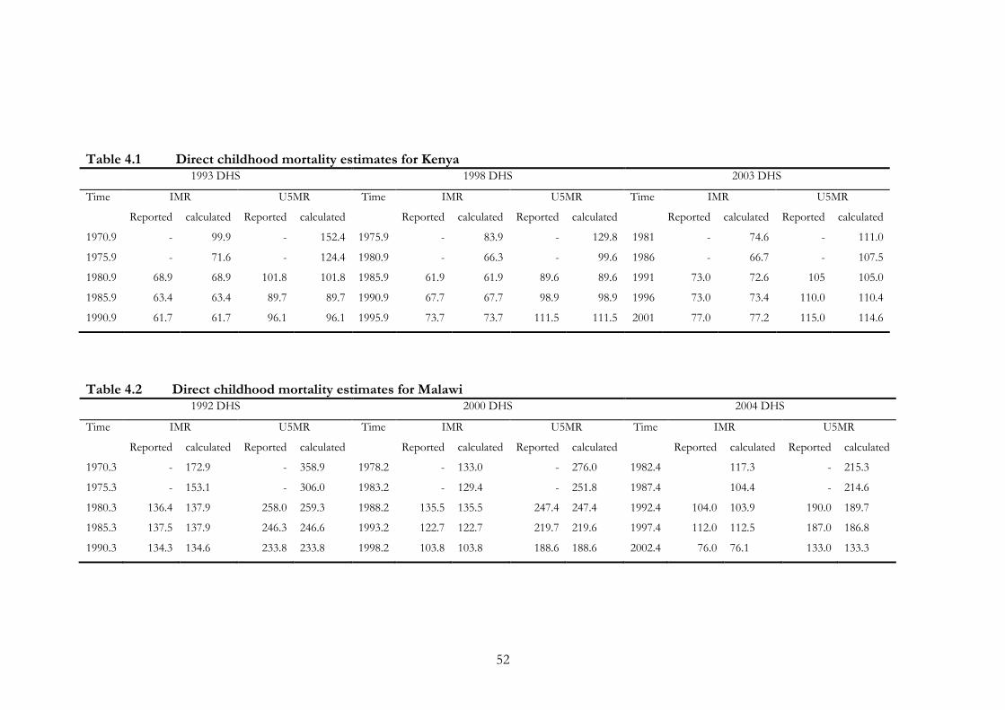
52
Table 4.1 Direct childhood mortality estimates for Kenya
1993 DHS 1998 DHS 2003 DHS
Time IMR U5MR Time IMR U5MR Time IMR U5MR
Reported calculated Reported calculated Reported calculated Reported calculated Reported calculated Reported calculated
1970.9 - 99.9 - 152.4 1975.9 - 83.9 - 129.8 1981 - 74.6 - 111.0
1975.9 - 71.6 - 124.4 1980.9 - 66.3 - 99.6 1986 - 66.7 - 107.5
1980.9 68.9 68.9 101.8 101.8 1985.9 61.9 61.9 89.6 89.6 1991 73.0 72.6 105 105.0
1985.9 63.4 63.4 89.7 89.7 1990.9 67.7 67.7 98.9 98.9 1996 73.0 73.4 110.0 110.4
1990.9 61.7 61.7 96.1 96.1 1995.9 73.7 73.7 111.5 111.5 2001 77.0 77.2 115.0 114.6
Table 4.2 Direct childhood mortality estimates for Malawi 1992 DHS 2000 DHS 2004 DHS
Time IMR U5MR Time IMR U5MR Time IMR U5MR
Reported calculated Reported calculated Reported calculated Reported calculated Reported calculated Reported calculated
1970.3 - 172.9 - 358.9 1978.2 - 133.0 - 276.0 1982.4 117.3 - 215.3
1975.3 - 153.1 - 306.0 1983.2 - 129.4 - 251.8 1987.4 104.4 - 214.6
1980.3 136.4 137.9 258.0 259.3 1988.2 135.5 135.5 247.4 247.4 1992.4 104.0 103.9 190.0 189.7
1985.3 137.5 137.9 246.3 246.6 1993.2 122.7 122.7 219.7 219.6 1997.4 112.0 112.5 187.0 186.8
1990.3 134.3 134.6 233.8 233.8 1998.2 103.8 103.8 188.6 188.6 2002.4 76.0 76.1 133.0 133.3
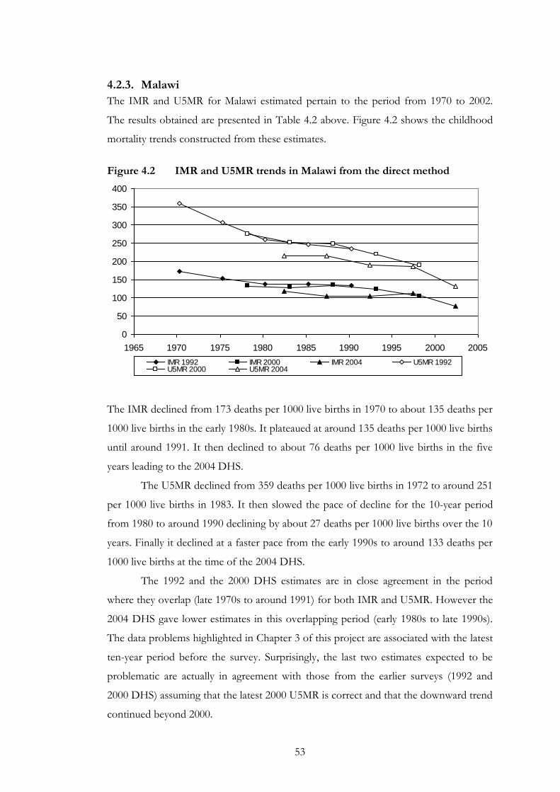
53
4.2.3. Malawi
The IMR and U5MR for Malawi estimated pertain to the period from 1970 to 2002.
The results obtained are presented in Table 4.2 above. Figure 4.2 shows the childhood
mortality trends constructed from these estimates.
Figure 4.2 IMR and U5MR trends in Malawi from the direct method
0
50
100
150
200
250
300
350
400
1965 1970 1975 1980 1985 1990 1995 2000 2005
IMR 1992 IMR 2000 IMR 2004 U5MR 1992U5MR 2000 U5MR 2004
The IMR declined from 173 deaths per 1000 live births in 1970 to about 135 deaths per
1000 live births in the early 1980s. It plateaued at around 135 deaths per 1000 live births
until around 1991. It then declined to about 76 deaths per 1000 live births in the five
years leading to the 2004 DHS.
The U5MR declined from 359 deaths per 1000 live births in 1972 to around 251
per 1000 live births in 1983. It then slowed the pace of decline for the 10-year period
from 1980 to around 1990 declining by about 27 deaths per 1000 live births over the 10
years. Finally it declined at a faster pace from the early 1990s to around 133 deaths per
1000 live births at the time of the 2004 DHS.
The 1992 and the 2000 DHS estimates are in close agreement in the period
where they overlap (late 1970s to around 1991) for both IMR and U5MR. However the
2004 DHS gave lower estimates in this overlapping period (early 1980s to late 1990s).
The data problems highlighted in Chapter 3 of this project are associated with the latest
ten-year period before the survey. Surprisingly, the last two estimates expected to be
problematic are actually in agreement with those from the earlier surveys (1992 and
2000 DHS) assuming that the latest 2000 U5MR is correct and that the downward trend
continued beyond 2000.
54
The lower estimates in the periods earlier than ten years before the 2004 DHS
could be due to omission of children who did not survive to the time of the 2004 DHS.
Mortality levels are higher in Malawi than in Kenya. U5MR experienced in Kenya over
the period from the early 1970s to the time of the 2003 DHS are at roughly similar
levels with the IMR in Malawi over the same period.
In Kenya the average difference between U5MR and the IMR has remained
generally constant over the period under review while in Malawi this difference has
been narrowing over time.
4.2.4. Indirect childhood mortality
For each of the datasets used, numbers of children ever born and children surviving (at
the time of the survey or census) were tabulated by five-year age groups of mothers.
The numbers of women in each of the five year age groups in the reproductive age
range (15-49) were also tabulated.
The Trussell version of the Brass children ever born, children surviving method
described in section 2.4.2.1 was applied to the tabulated numbers of children ever born
and children surviving.
The North family in the Princeton model life table system was used for both
Kenya and Malawi. It was decided, on the basis of previous studies, that the North
family was the most suitable model life table for Kenya (Population Division United
Nations Secretariat, 1990) and Malawi (Malawi National Statistical Office, 2002). The
West family, which is recommended when there is no other information on the
appropriate model life table family to use, was tried (results not shown). It gave no clear
advantage over the North family in both countries, if anything, it gave more volatile
trends.
The results obtained from the application of the Trussell variant of the Brass
children ever born children surviving technique are given below in
Table 4.3 and Table 4.4.
4.2.5. Kenya
The Kenya childhood mortality trends from indirect estimates are for the period from
1979 to 2001. The trends constructed from these indirect estimates are shown in Figure
4.3 below.
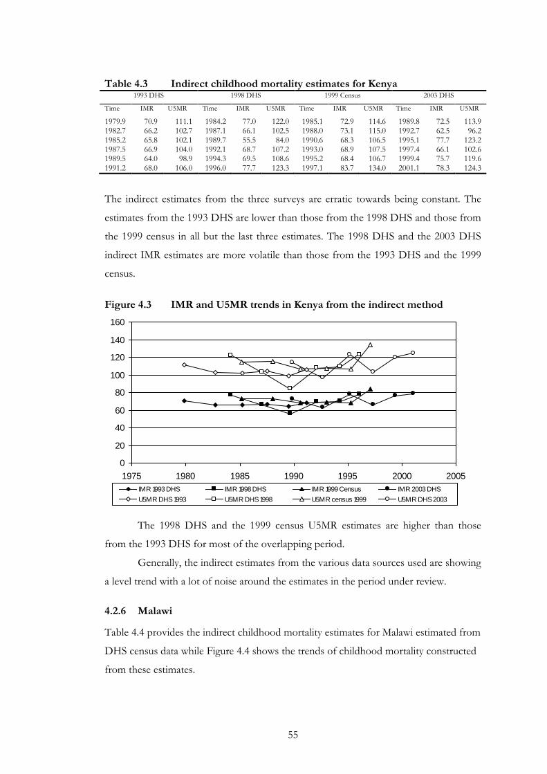
55
Table 4.3 Indirect childhood mortality estimates for Kenya
1993 DHS 1998 DHS 1999 Census 2003 DHS
Time IMR U5MR Time IMR U5MR Time IMR U5MR Time IMR U5MR
1979.9 70.9 111.1 1984.2 77.0 122.0 1985.1 72.9 114.6 1989.8 72.5 113.9 1982.7 66.2 102.7 1987.1 66.1 102.5 1988.0 73.1 115.0 1992.7 62.5 96.2 1985.2 65.8 102.1 1989.7 55.5 84.0 1990.6 68.3 106.5 1995.1 77.7 123.2 1987.5 66.9 104.0 1992.1 68.7 107.2 1993.0 68.9 107.5 1997.4 66.1 102.6 1989.5 64.0 98.9 1994.3 69.5 108.6 1995.2 68.4 106.7 1999.4 75.7 119.6 1991.2 68.0 106.0 1996.0 77.7 123.3 1997.1 83.7 134.0 2001.1 78.3 124.3
The indirect estimates from the three surveys are erratic towards being constant. The
estimates from the 1993 DHS are lower than those from the 1998 DHS and those from
the 1999 census in all but the last three estimates. The 1998 DHS and the 2003 DHS
indirect IMR estimates are more volatile than those from the 1993 DHS and the 1999
census.
Figure 4.3 IMR and U5MR trends in Kenya from the indirect method
0
20
40
60
80
100
120
140
160
1975 1980 1985 1990 1995 2000 2005
IMR 1993 DHS IMR 1998 DHS IMR 1999 Census IMR 2003 DHS
U5MR DHS 1993 U5MR DHS 1998 U5MR census 1999 U5MR DHS 2003
The 1998 DHS and the 1999 census U5MR estimates are higher than those
from the 1993 DHS for most of the overlapping period.
Generally, the indirect estimates from the various data sources used are showing
a level trend with a lot of noise around the estimates in the period under review.
4.2.6 Malawi
Table 4.4 provides the indirect childhood mortality estimates for Malawi estimated from
DHS census data while Figure 4.4 shows the trends of childhood mortality constructed
from these estimates.
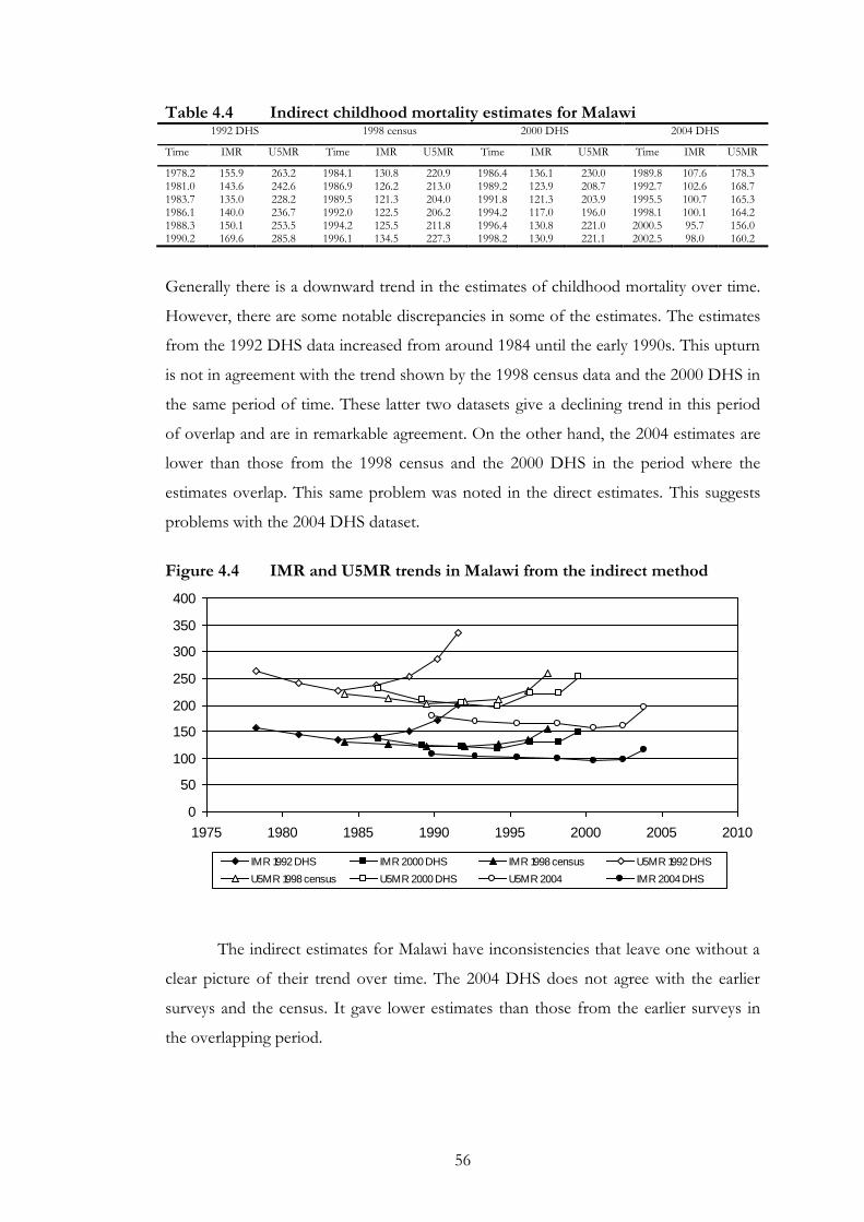
56
Table 4.4 Indirect childhood mortality estimates for Malawi 1992 DHS 1998 census 2000 DHS 2004 DHS
Time IMR U5MR Time IMR U5MR Time IMR U5MR Time IMR U5MR
1978.2 155.9 263.2 1984.1 130.8 220.9 1986.4 136.1 230.0 1989.8 107.6 178.3 1981.0 143.6 242.6 1986.9 126.2 213.0 1989.2 123.9 208.7 1992.7 102.6 168.7 1983.7 135.0 228.2 1989.5 121.3 204.0 1991.8 121.3 203.9 1995.5 100.7 165.3 1986.1 140.0 236.7 1992.0 122.5 206.2 1994.2 117.0 196.0 1998.1 100.1 164.2 1988.3 150.1 253.5 1994.2 125.5 211.8 1996.4 130.8 221.0 2000.5 95.7 156.0 1990.2 169.6 285.8 1996.1 134.5 227.3 1998.2 130.9 221.1 2002.5 98.0 160.2
Generally there is a downward trend in the estimates of childhood mortality over time.
However, there are some notable discrepancies in some of the estimates. The estimates
from the 1992 DHS data increased from around 1984 until the early 1990s. This upturn
is not in agreement with the trend shown by the 1998 census data and the 2000 DHS in
the same period of time. These latter two datasets give a declining trend in this period
of overlap and are in remarkable agreement. On the other hand, the 2004 estimates are
lower than those from the 1998 census and the 2000 DHS in the period where the
estimates overlap. This same problem was noted in the direct estimates. This suggests
problems with the 2004 DHS dataset.
Figure 4.4 IMR and U5MR trends in Malawi from the indirect method
0
50
100
150
200
250
300
350
400
1975 1980 1985 1990 1995 2000 2005 2010
IMR 1992 DHS IMR 2000 DHS IMR 1998 census U5MR 1992 DHS
U5MR 1998 census U5MR 2000 DHS U5MR 2004 IMR 2004 DHS
The indirect estimates for Malawi have inconsistencies that leave one without a
clear picture of their trend over time. The 2004 DHS does not agree with the earlier
surveys and the census. It gave lower estimates than those from the earlier surveys in
the overlapping period.
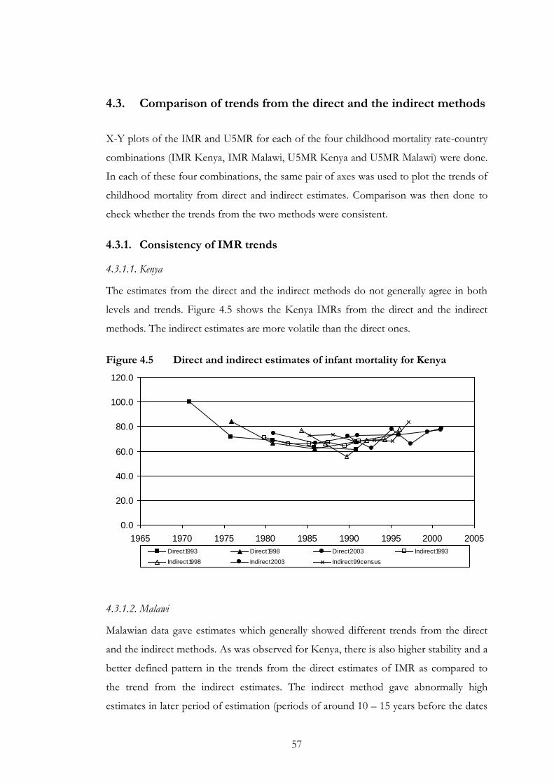
57
4.3. Comparison of trends from the direct and the indirect methods
X-Y plots of the IMR and U5MR for each of the four childhood mortality rate-country
combinations (IMR Kenya, IMR Malawi, U5MR Kenya and U5MR Malawi) were done.
In each of these four combinations, the same pair of axes was used to plot the trends of
childhood mortality from direct and indirect estimates. Comparison was then done to
check whether the trends from the two methods were consistent.
4.3.1. Consistency of IMR trends
4.3.1.1. Kenya
The estimates from the direct and the indirect methods do not generally agree in both
levels and trends. Figure 4.5 shows the Kenya IMRs from the direct and the indirect
methods. The indirect estimates are more volatile than the direct ones.
Figure 4.5 Direct and indirect estimates of infant mortality for Kenya
0.0
20.0
40.0
60.0
80.0
100.0
120.0
1965 1970 1975 1980 1985 1990 1995 2000 2005
Direct1993 Direct1998 Direct2003 Indirect1993
Indirect1998 Indirect2003 Indirect99census
4.3.1.2. Malawi
Malawian data gave estimates which generally showed different trends from the direct
and the indirect methods. As was observed for Kenya, there is also higher stability and a
better defined pattern in the trends from the direct estimates of IMR as compared to
the trend from the indirect estimates. The indirect method gave abnormally high
estimates in later period of estimation (periods of around 10 – 15 years before the dates
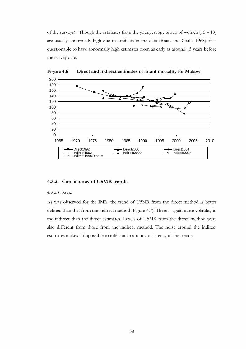
58
of the surveys). Though the estimates from the youngest age group of women (15 – 19)
are usually abnormally high due to artefacts in the data (Brass and Coale, 1968), it is
questionable to have abnormally high estimates from as early as around 15 years before
the survey date.
Figure 4.6 Direct and indirect estimates of infant mortality for Malawi
0
20
40
60
80
100
120
140
160
180
200
1965 1970 1975 1980 1985 1990 1995 2000 2005 2010
Direct1992 Direct2000 Direct2004Indirect1992 Indirect2000 Indirect2004Indirect1998Census
4.3.2. Consistency of U5MR trends
4.3.2.1. Kenya
As was observed for the IMR, the trend of U5MR from the direct method is better
defined than that from the indirect method (Figure 4.7). There is again more volatility in
the indirect than the direct estimates. Levels of U5MR from the direct method were
also different from those from the indirect method. The noise around the indirect
estimates makes it impossible to infer much about consistency of the trends.
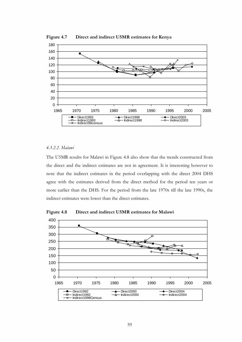
59
Figure 4.7 Direct and indirect U5MR estimates for Kenya
0
20
40
60
80
100
120
140
160
180
1965 1970 1975 1980 1985 1990 1995 2000 2005
Direct1993 Direct1998 Direct2003Indirect1993 Indirect1998 Indirect2003Indirect99census
4.3.2.2. Malawi
The U5MR results for Malawi in Figure 4.8 also show that the trends constructed from
the direct and the indirect estimates are not in agreement. It is interesting however to
note that the indirect estimates in the period overlapping with the direct 2004 DHS
agree with the estimates derived from the direct method for the period ten years or
more earlier than the DHS. For the period from the late 1970s till the late 1990s, the
indirect estimates were lower than the direct estimates.
Figure 4.8 Direct and indirect U5MR estimates for Malawi
0
50
100
150
200
250
300
350
400
1965 1970 1975 1980 1985 1990 1995 2000 2005
Direct1992 Direct2000 Direct2004Indirect1992 Indirect2000 Indirect2004Indirect1998Census
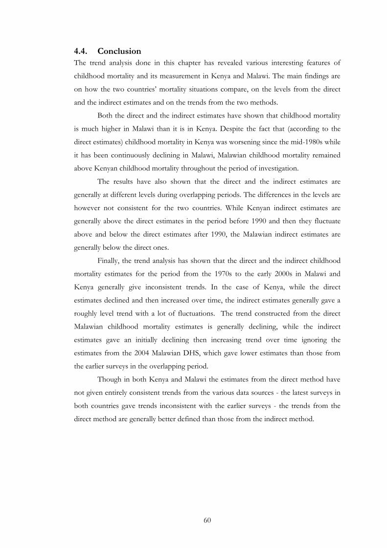
60
4.4. Conclusion
The trend analysis done in this chapter has revealed various interesting features of
childhood mortality and its measurement in Kenya and Malawi. The main findings are
on how the two countries’ mortality situations compare, on the levels from the direct
and the indirect estimates and on the trends from the two methods.
Both the direct and the indirect estimates have shown that childhood mortality
is much higher in Malawi than it is in Kenya. Despite the fact that (according to the
direct estimates) childhood mortality in Kenya was worsening since the mid-1980s while
it has been continuously declining in Malawi, Malawian childhood mortality remained
above Kenyan childhood mortality throughout the period of investigation.
The results have also shown that the direct and the indirect estimates are
generally at different levels during overlapping periods. The differences in the levels are
however not consistent for the two countries. While Kenyan indirect estimates are
generally above the direct estimates in the period before 1990 and then they fluctuate
above and below the direct estimates after 1990, the Malawian indirect estimates are
generally below the direct ones.
Finally, the trend analysis has shown that the direct and the indirect childhood
mortality estimates for the period from the 1970s to the early 2000s in Malawi and
Kenya generally give inconsistent trends. In the case of Kenya, while the direct
estimates declined and then increased over time, the indirect estimates generally gave a
roughly level trend with a lot of fluctuations. The trend constructed from the direct
Malawian childhood mortality estimates is generally declining, while the indirect
estimates gave an initially declining then increasing trend over time ignoring the
estimates from the 2004 Malawian DHS, which gave lower estimates than those from
the earlier surveys in the overlapping period.
Though in both Kenya and Malawi the estimates from the direct method have
not given entirely consistent trends from the various data sources - the latest surveys in
both countries gave trends inconsistent with the earlier surveys - the trends from the
direct method are generally better defined than those from the indirect method.
61
5. HIV population attributable fraction (PAF)
5.1. Introduction
This chapter describes the method used to quantify the impact of HIV/AIDS on
childhood mortality (HIV PAF). It also presents the results obtained from the
application of the method to Kenyan and Malawian data. The formula used for the HIV
PAF estimation in the current study is the same as the one that was used in the Zaba
method (Equation 2-1). The difference between the two methods (the current
methodology and the method used by Zaba and colleagues) is in the overall mortality
and the mortality of uninfected children used in the formula. Zaba measured both the
direct and the indirect effects of HIV/ AIDS on childhood mortality while this study
only measures the direct effect. Section 5.2 considers the overall childhood mortality
estimates used in the current study. Section 5.3 presents the estimates of mortality of
the uninfected children. Section 5.4 presents the estimates of HIV PAF. Finally, section
5.5 gives the conclusion.
5.2. Overall childhood mortality
The overall childhood mortality estimates used in this study were obtained as follows:
First, direct childhood mortality estimates from the Kenya 2003 and the Malawi 2004
DHS were confirmed as described before in sub-section 4.2.1. Second, the confirmed
estimates were adjusted for bias due to HIV/ AIDS (1 per cent and 5 per cent
respectively for IMR and U5MR) as suggested by Zaba, Marston and Floyd (2003).
Third, an alternative set of overall childhood mortality estimates was derived by adding
expected direct childhood AIDS deaths to non-AIDS deaths (mortality of the children
of HIV negative mothers). Fourth, an average of the two estimates was obtained and
was used as the overall childhood mortality. The overall childhood mortality estimates
are tabulated in Table 5.1 below.
IMR from all causes (overall IMR) for Kenya in 2003 was slightly higher (81 per
1000) than the IMR from all causes in Malawi in 2004 (80 per 1000). The overall
U5MR for Kenya (126 per 1000) was however lower than that for Malawi (140 per
1000) with the result that the contribution of child mortality to U5MR in Malawi was
higher than in Kenya.
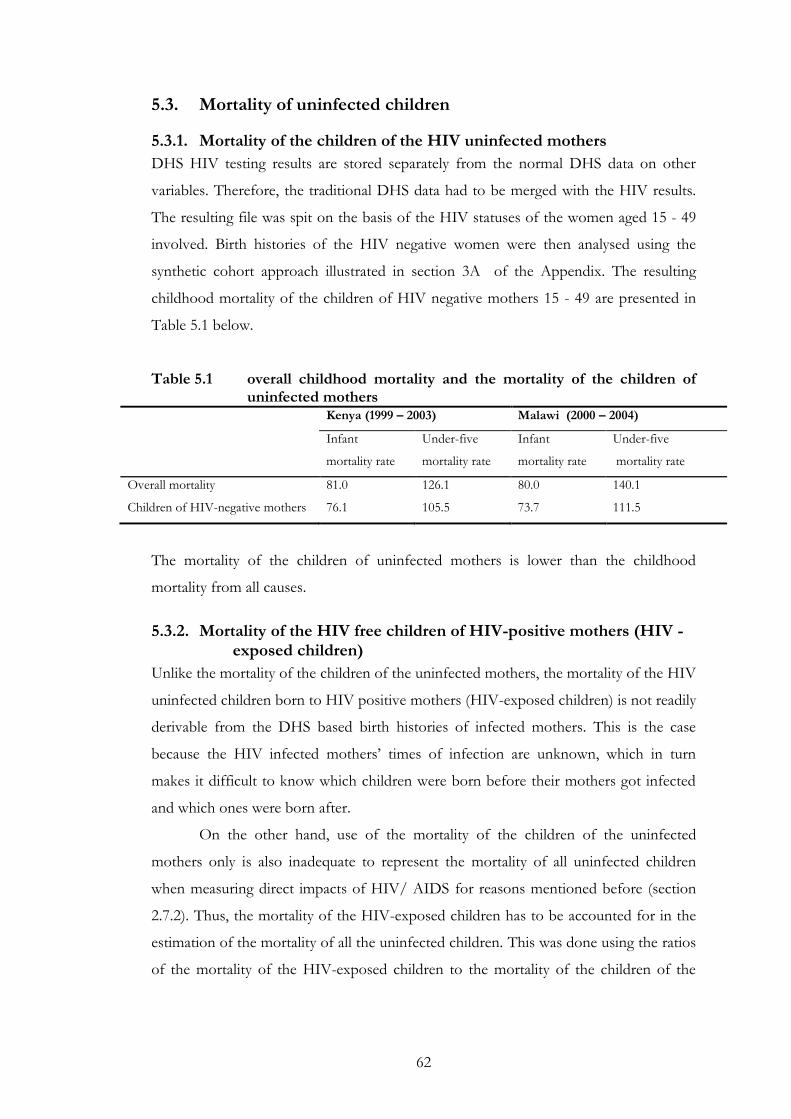
62
5.3. Mortality of uninfected children
5.3.1. Mortality of the children of the HIV uninfected mothers
DHS HIV testing results are stored separately from the normal DHS data on other
variables. Therefore, the traditional DHS data had to be merged with the HIV results.
The resulting file was spit on the basis of the HIV statuses of the women aged 15 - 49
involved. Birth histories of the HIV negative women were then analysed using the
synthetic cohort approach illustrated in section 3A of the Appendix. The resulting
childhood mortality of the children of HIV negative mothers 15 - 49 are presented in
Table 5.1 below.
Table 5.1 overall childhood mortality and the mortality of the children of uninfected mothers
Kenya (1999 – 2003) Malawi (2000 – 2004)
Infant
mortality rate
Under-five
mortality rate
Infant
mortality rate
Under-five
mortality rate
Overall mortality 81.0 126.1 80.0 140.1
Children of HIV-negative mothers 76.1 105.5 73.7 111.5
The mortality of the children of uninfected mothers is lower than the childhood
mortality from all causes.
5.3.2. Mortality of the HIV free children of HIV-positive mothers (HIV -exposed children)
Unlike the mortality of the children of the uninfected mothers, the mortality of the HIV
uninfected children born to HIV positive mothers (HIV-exposed children) is not readily
derivable from the DHS based birth histories of infected mothers. This is the case
because the HIV infected mothers’ times of infection are unknown, which in turn
makes it difficult to know which children were born before their mothers got infected
and which ones were born after.
On the other hand, use of the mortality of the children of the uninfected
mothers only is also inadequate to represent the mortality of all uninfected children
when measuring direct impacts of HIV/ AIDS for reasons mentioned before (section
2.7.2). Thus, the mortality of the HIV-exposed children has to be accounted for in the
estimation of the mortality of all the uninfected children. This was done using the ratios
of the mortality of the HIV-exposed children to the mortality of the children of the
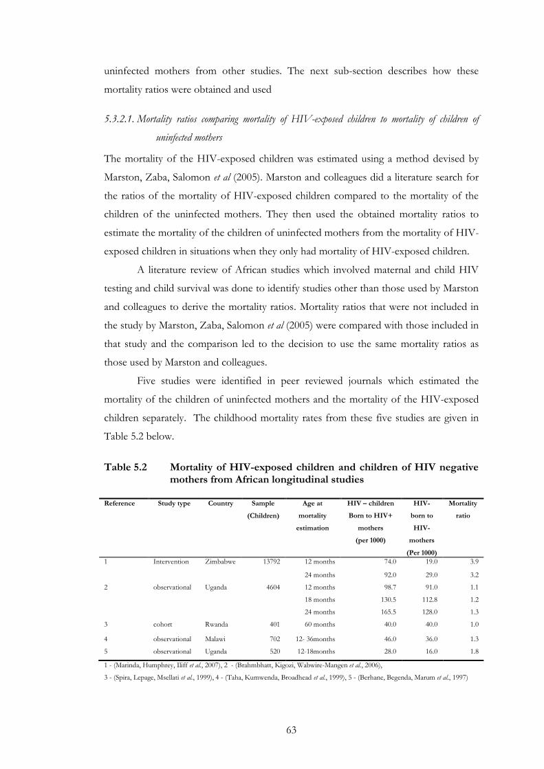
63
uninfected mothers from other studies. The next sub-section describes how these
mortality ratios were obtained and used
5.3.2.1. Mortality ratios comparing mortality of HIV-exposed children to mortality of children of
uninfected mothers
The mortality of the HIV-exposed children was estimated using a method devised by
Marston, Zaba, Salomon et al (2005). Marston and colleagues did a literature search for
the ratios of the mortality of HIV-exposed children compared to the mortality of the
children of the uninfected mothers. They then used the obtained mortality ratios to
estimate the mortality of the children of uninfected mothers from the mortality of HIV-
exposed children in situations when they only had mortality of HIV-exposed children.
A literature review of African studies which involved maternal and child HIV
testing and child survival was done to identify studies other than those used by Marston
and colleagues to derive the mortality ratios. Mortality ratios that were not included in
the study by Marston, Zaba, Salomon et al (2005) were compared with those included in
that study and the comparison led to the decision to use the same mortality ratios as
those used by Marston and colleagues.
Five studies were identified in peer reviewed journals which estimated the
mortality of the children of uninfected mothers and the mortality of the HIV-exposed
children separately. The childhood mortality rates from these five studies are given in
Table 5.2 below.
Table 5.2 Mortality of HIV-exposed children and children of HIV negative
mothers from African longitudinal studies Reference Study type Country Sample
(Children)
Age at
mortality
estimation
HIV – children
Born to HIV+
mothers
(per 1000)
HIV-
born to
HIV-
mothers
(Per 1000)
Mortality
ratio
1 Intervention Zimbabwe 13792 12 months 74.0 19.0 3.9
24 months 92.0 29.0 3.2
2 observational Uganda 4604 12 months 98.7 91.0 1.1
18 months 130.5 112.8 1.2
24 months 165.5 128.0 1.3
3 cohort Rwanda 401 60 months 40.0 40.0 1.0
4 observational Malawi 702 12- 36months 46.0 36.0 1.3
5 observational Uganda 520 12-18months 28.0 16.0 1.8
1 - (Marinda, Humphrey, Iliff et al., 2007), 2 - (Brahmbhatt, Kigozi, Wabwire-Mangen et al., 2006),
3 - (Spira, Lepage, Msellati et al., 1999), 4 - (Taha, Kumwenda, Broadhead et al., 1999), 5 - (Berhane, Begenda, Marum et al., 1997)
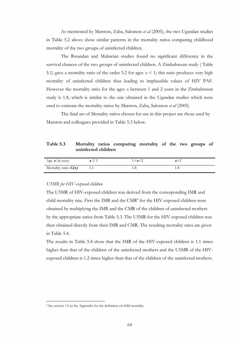
64
As mentioned by Marston, Zaba, Salomon et al (2005), the two Ugandan studies
in Table 5.2 above show similar patterns in the mortality ratios comparing childhood
mortality of the two groups of uninfected children.
The Rwandan and Malawian studies found no significant difference in the
survival chances of the two groups of uninfected children. A Zimbabwean study ( Table
5.1) gave a mortality ratio of the order 3.2 for ages x < 1; this ratio produces very high
mortality of uninfected children thus leading to implausible values of HIV PAF.
However the mortality ratio for the ages x between 1 and 2 years in the Zimbabwean
study is 1.8, which is similar to the one obtained in the Ugandan studies which were
used to estimate the mortality ratios by Marston, Zaba, Salomon et al (2005)
The final set of Mortality ratios chosen for use in this project are those used by
Marston and colleagues provided in Table 5.3 below.
Table 5.3 Mortality ratios comparing mortality of the two groups of
uninfected children Age x (in years) x ≤ 1 1<x<2 x>2
Mortality ratio C(x) 1.1 1.8 1.8
U5MR for HIV-exposed children
The U5MR of HIV-exposed children was derived from the corresponding IMR and
child mortality rate. First the IMR and the CMR4 for the HIV-exposed children were
obtained by multiplying the IMR and the CMR of the children of uninfected mothers
by the appropriate ratios from Table 5.3. The U5MR for the HIV-exposed children was
then obtained directly from their IMR and CMR. The resulting mortality rates are given
in Table 5.4.
The results in Table 5.4 show that the IMR of the HIV-exposed children is 1.1 times
higher than that of the children of the uninfected mothers and the U5MR of the HIV-
exposed children is 1.2 times higher than that of the children of the uninfected mothers.
4 See section 1A in the Appendix for the definition of child mortality.
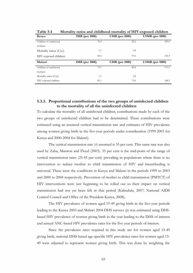
65
Table 5.4 Mortality ratios and childhood mortality of HIV-exposed children Kenya IMR (per 1000) CMR (per 1000) U5MR (per 1000)
Children of uninfected
mothers
76.0 32.0 105.0
Mortality ratios (C(x)) 1.1 1.8
HIV-exposed children 83.6 57.6 136.4
Malawi IMR (per 1000) CMR (per 1000) U5MR (per 1000)
Children of uninfected
mothers
73.7 40.8 111.5
Mortality ratios (C(x)) 1.1 1.8
HIV-exposed children 81.1 73.4 148.5
5.3.3. Proportional contributions of the two groups of uninfected children to the mortality of all the uninfected children
To calculate the mortality of all uninfected children, contributions made by each of the
two groups of uninfected children had to be determined. These contributions were
estimated using an assumed vertical transmission rate and estimates of HIV prevalence
among women giving birth in the five-year periods under consideration (1999-2003 for
Kenya and 2000-2004 for Malawi).
The vertical transmission rate (v) assumed is 35 per cent. This same rate was also
used by Zaba, Marston and Floyd (2003). 35 per cent is the mid-point of the range of
vertical transmission rates (25-45 per cent) prevailing in populations where there is no
intervention to reduce mother to child transmission of HIV and breastfeeding is
universal. These were the conditions in Kenya and Malawi in the periods 1999 to 2003
and 2000 to 2004 respectively. Prevention of mother to child transmission (PMTCT) of
HIV interventions were just beginning to be rolled out so their impact on vertical
transmission had not yet been felt in that period (Kabudula, 2007; National AIDS
Control Council and Office of the President Kenya, 2008).
The HIV prevalence of women aged 15-49 giving birth in the five-year periods
leading to the Kenya 2003 and Malawi 2004 DHS surveys (p) was estimated using DHS-
based HIV prevalence of women giving birth in the year leading to the DHS of interest
and annual ANC-based HIV prevalence rates for the five year periods of interest.
Since the prevalence rates required in this study are for women aged 15-49
giving birth, national DHS-based age-specific HIV prevalence rates for women aged 15-
49 were adjusted to represent women giving birth. This was done by weighting the
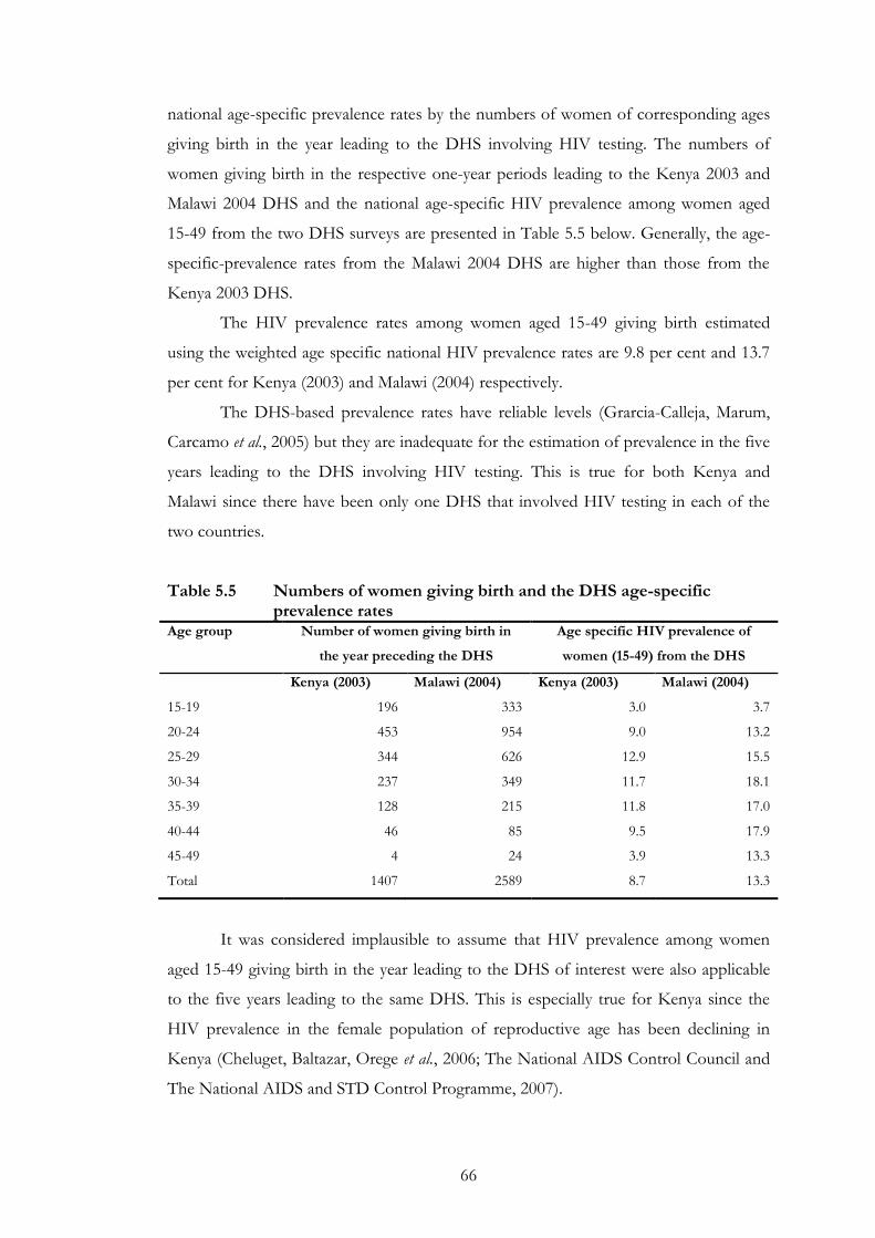
66
national age-specific prevalence rates by the numbers of women of corresponding ages
giving birth in the year leading to the DHS involving HIV testing. The numbers of
women giving birth in the respective one-year periods leading to the Kenya 2003 and
Malawi 2004 DHS and the national age-specific HIV prevalence among women aged
15-49 from the two DHS surveys are presented in Table 5.5 below. Generally, the age-
specific-prevalence rates from the Malawi 2004 DHS are higher than those from the
Kenya 2003 DHS.
The HIV prevalence rates among women aged 15-49 giving birth estimated
using the weighted age specific national HIV prevalence rates are 9.8 per cent and 13.7
per cent for Kenya (2003) and Malawi (2004) respectively.
The DHS-based prevalence rates have reliable levels (Grarcia-Calleja, Marum,
Carcamo et al., 2005) but they are inadequate for the estimation of prevalence in the five
years leading to the DHS involving HIV testing. This is true for both Kenya and
Malawi since there have been only one DHS that involved HIV testing in each of the
two countries.
Table 5.5 Numbers of women giving birth and the DHS age-specific prevalence rates
Age group Number of women giving birth in
the year preceding the DHS
Age specific HIV prevalence of
women (15-49) from the DHS
Kenya (2003) Malawi (2004) Kenya (2003) Malawi (2004)
15-19 196 333 3.0 3.7
20-24 453 954 9.0 13.2
25-29 344 626 12.9 15.5
30-34 237 349 11.7 18.1
35-39 128 215 11.8 17.0
40-44 46 85 9.5 17.9
45-49 4 24 3.9 13.3
Total 1407 2589 8.7 13.3
It was considered implausible to assume that HIV prevalence among women
aged 15-49 giving birth in the year leading to the DHS of interest were also applicable
to the five years leading to the same DHS. This is especially true for Kenya since the
HIV prevalence in the female population of reproductive age has been declining in
Kenya (Cheluget, Baltazar, Orege et al., 2006; The National AIDS Control Council and
The National AIDS and STD Control Programme, 2007).
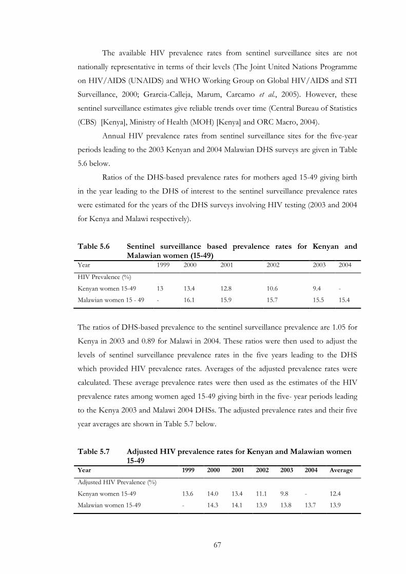
67
The available HIV prevalence rates from sentinel surveillance sites are not
nationally representative in terms of their levels (The Joint United Nations Programme
on HIV/AIDS (UNAIDS) and WHO Working Group on Global HIV/AIDS and STI
Surveillance, 2000; Grarcia-Calleja, Marum, Carcamo et al., 2005). However, these
sentinel surveillance estimates give reliable trends over time (Central Bureau of Statistics
(CBS) [Kenya], Ministry of Health (MOH) [Kenya] and ORC Macro, 2004).
Annual HIV prevalence rates from sentinel surveillance sites for the five-year
periods leading to the 2003 Kenyan and 2004 Malawian DHS surveys are given in Table
5.6 below.
Ratios of the DHS-based prevalence rates for mothers aged 15-49 giving birth
in the year leading to the DHS of interest to the sentinel surveillance prevalence rates
were estimated for the years of the DHS surveys involving HIV testing (2003 and 2004
for Kenya and Malawi respectively).
Table 5.6 Sentinel surveillance based prevalence rates for Kenyan and Malawian women (15-49)
Year 1999 2000 2001 2002 2003 2004
HIV Prevalence (%)
Kenyan women 15-49 13 13.4 12.8 10.6 9.4 -
Malawian women 15 - 49 - 16.1 15.9 15.7 15.5 15.4
The ratios of DHS-based prevalence to the sentinel surveillance prevalence are 1.05 for
Kenya in 2003 and 0.89 for Malawi in 2004. These ratios were then used to adjust the
levels of sentinel surveillance prevalence rates in the five years leading to the DHS
which provided HIV prevalence rates. Averages of the adjusted prevalence rates were
calculated. These average prevalence rates were then used as the estimates of the HIV
prevalence rates among women aged 15-49 giving birth in the five- year periods leading
to the Kenya 2003 and Malawi 2004 DHSs. The adjusted prevalence rates and their five
year averages are shown in Table 5.7 below.
Table 5.7 Adjusted HIV prevalence rates for Kenyan and Malawian women 15-49
Year 1999 2000 2001 2002 2003 2004 Average
Adjusted HIV Prevalence (%)
Kenyan women 15-49 13.6 14.0 13.4 11.1 9.8 - 12.4
Malawian women 15-49 - 14.3 14.1 13.9 13.8 13.7 13.9
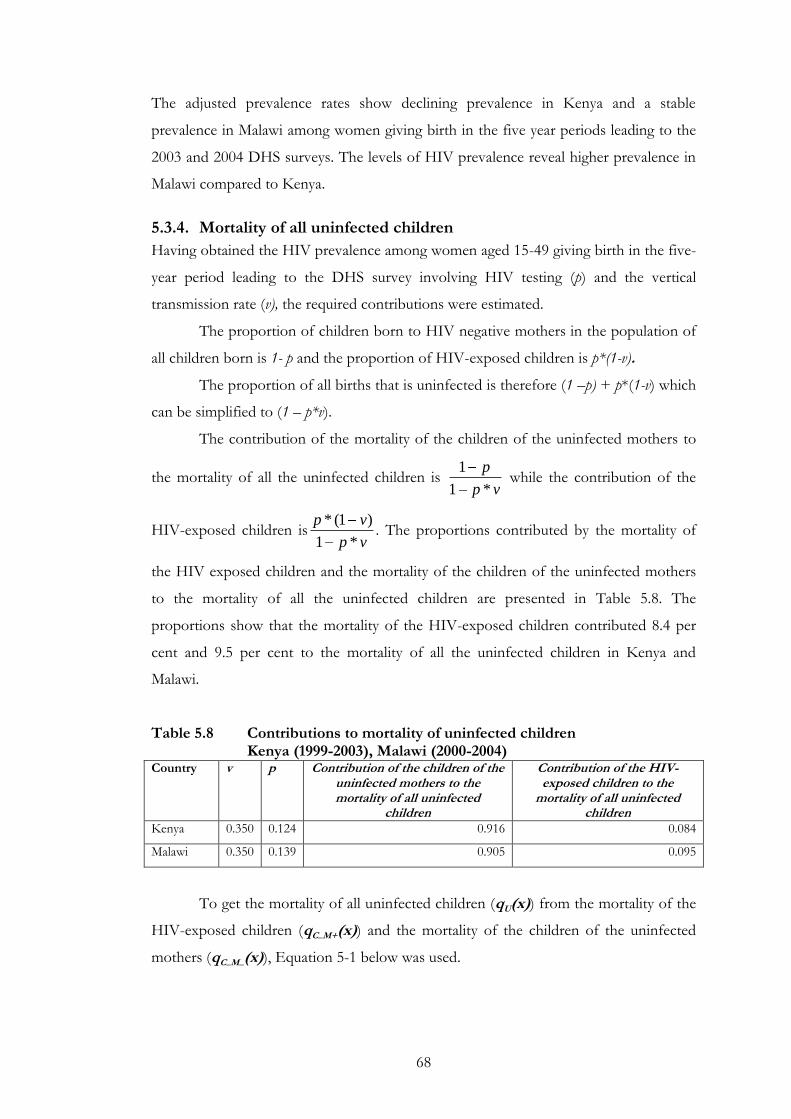
68
The adjusted prevalence rates show declining prevalence in Kenya and a stable
prevalence in Malawi among women giving birth in the five year periods leading to the
2003 and 2004 DHS surveys. The levels of HIV prevalence reveal higher prevalence in
Malawi compared to Kenya.
5.3.4. Mortality of all uninfected children
Having obtained the HIV prevalence among women aged 15-49 giving birth in the five-
year period leading to the DHS survey involving HIV testing (p) and the vertical
transmission rate (v), the required contributions were estimated.
The proportion of children born to HIV negative mothers in the population of
all children born is 1- p and the proportion of HIV-exposed children is p*(1-v).
The proportion of all births that is uninfected is therefore (1 –p) + p*(1-v) which
can be simplified to (1 – p*v).
The contribution of the mortality of the children of the uninfected mothers to
the mortality of all the uninfected children is vp
p
*1
1 while the contribution of the
HIV-exposed children isvp
vp
*1
)1(*. The proportions contributed by the mortality of
the HIV exposed children and the mortality of the children of the uninfected mothers
to the mortality of all the uninfected children are presented in Table 5.8. The
proportions show that the mortality of the HIV-exposed children contributed 8.4 per
cent and 9.5 per cent to the mortality of all the uninfected children in Kenya and
Malawi.
Table 5.8 Contributions to mortality of uninfected children Kenya (1999-2003), Malawi (2000-2004)
Country v p Contribution of the children of the uninfected mothers to the mortality of all uninfected
children
Contribution of the HIV-exposed children to the
mortality of all uninfected children
Kenya 0.350 0.124 0.916 0.084
Malawi 0.350 0.139 0.905 0.095
To get the mortality of all uninfected children (qU(x)) from the mortality of the
HIV-exposed children (qC_M+(x)) and the mortality of the children of the uninfected
mothers (qC_M_(x)), Equation 5-1 below was used.
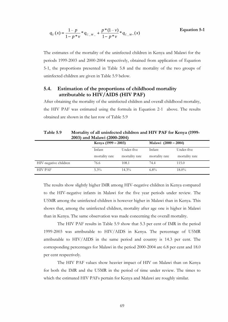
69
)(**1
)1(**
*1
1)( ___ xq
vp
vpq
vp
pxq MCMCU
Equation 5-1
The estimates of the mortality of the uninfected children in Kenya and Malawi for the
periods 1999-2003 and 2000-2004 respectively, obtained from application of Equation
5-1, the proportions presented in Table 5.8 and the mortality of the two groups of
uninfected children are given in Table 5.9 below.
5.4. Estimation of the proportions of childhood mortality attributable to HIV/AIDS (HIV PAF)
After obtaining the mortality of the uninfected children and overall childhood mortality,
the HIV PAF was estimated using the formula in Equation 2-1 above. The results
obtained are shown in the last row of Table 5.9
Table 5.9 Mortality of all uninfected children and HIV PAF for Kenya (1999-2003) and Malawi (2000-2004)
Kenya (1999 – 2003) Malawi (2000 – 2004)
Infant
mortality rate
Under-five
mortality rate
Infant
mortality rate
Under-five
mortality rate
HIV-negative children 76.6 108.1 74.4 115.0
HIV PAF 5.3% 14.3% 6.8% 18.0%
The results show slightly higher IMR among HIV-negative children in Kenya compared
to the HIV-negative infants in Malawi for the five year periods under review. The
U5MR among the uninfected children is however higher in Malawi than in Kenya. This
shows that, among the uninfected children, mortality after age one is higher in Malawi
than in Kenya. The same observation was made concerning the overall mortality.
The HIV PAF results in Table 5.9 show that 5.3 per cent of IMR in the period
1999-2003 was attributable to HIV/AIDS in Kenya. The percentage of U5MR
attributable to HIV/AIDS in the same period and country is 14.3 per cent. The
corresponding percentages for Malawi in the period 2000-2004 are 6.8 per cent and 18.0
per cent respectively.
The HIV PAF values show heavier impact of HIV on Malawi than on Kenya
for both the IMR and the U5MR in the period of time under review. The times to
which the estimated HIV PAFs pertain for Kenya and Malawi are roughly similar.
70
5.5. Conclusion
In this chapter, childhood mortality HIV PAF has been estimated for Kenya in the
period 1999-2003 and 2000-2004 for Malawi. The data used for the estimation are
largely from DHSes involving HIV testing among women aged 15 - 49. In addition to
the DHS data, sentinel surveillance HIV prevalence rates and results from African
longitudinal studies were used.
The method used has accounted for HIV prevalence trends in the five-year
periods of interest and the mortality difference between HIV-exposed children and
children of uninfected mothers. The results obtained show that generally childhood
mortality was higher in Malawi than in Kenya in the period 1999 to 2004. The results
also show that the impact of HIV is higher on U5MR than on IMR. In both Kenya and
Malawi, the percentage of mortality attributable to HIV/AIDS was lower among infants
compared to the percentages among all children less than five. This means that more
AIDS attributable deaths are happening in the period from age one to age five than
those happening in the first year of life.
71
6. Discussion and conclusions
6.1. Introduction
The aims of this study were to check the consistency of the childhood mortality trends
constructed from direct and indirect methods in high HIV prevalence settings, and to
calculate HIV PAF using DHS data and results from African longitudinal studies. This
chapter discusses the extent to which the results obtained from the data analysis meet
the goals of the study. It also provides the main conclusions drawn from the study. The
organization of the chapter is as follows: Section 6.2 considers the results of the
comparison of the trends from the direct and the indirect methods. Section 6.3 looks at
the estimates of the HIV PAF obtained. Section 6.4 gives the limitations of the study.
Finally, section 6.5 gives the conclusions made from the study and recommendations
for further studies.
6.2. Childhood mortality trends from the direct and the indirect methods
The comparison of the trends of direct and indirect estimates of childhood mortality
suggests that the two methods give different trends. The trends from the direct method
are more clearly defined compared to those from the indirect method which have a lot
of noise around them.
The levels of childhood mortality from the two methods are different. This
observation is in accord with the results from the analysis of levels of infant mortality
done by Adetunji (1996). Adetunji mainly used statistical analysis of the levels of infant
mortality, while this study uses graphical analysis. The differences in the levels require
careful attention when constructing trends of childhood mortality using a mixture of
direct and indirect estimates.
The differences in levels of the direct and the indirect estimates are not
consistent between the two countries reviewed. While the direct estimates are generally
lower than the indirect estimates in the case of Kenya, the direct estimates for Malawi
are generally at higher levels than indirect ones. Kenya indirect estimates are also more
volatile than the Malawian indirect estimates. It appears that the fluctuations are not due
to the inherent properties of the indirect method (since they are absent in the Malawi
estimates). The causes of these fluctuations require further investigation.
72
Though Malawi is showing higher childhood mortality than Kenya, childhood
mortality is improving over time in Malawi while it has been increasing in Kenya since
the mid 1980s. It is more useful to analyse not only levels of childhood mortality at a
point in time but to also consider trends to identify countries which are improving over
time and vice versa. The continual decline in the childhood mortality for Malawi most
likely has to do with the fact that Malawi is coming off a high base, may have kept
declining due to improvement in background mortality not necessarily effecting control
of the effect of HIV/AIDS on childhood mortality.
The difference in the levels of infant mortality and under-five mortality is
known to narrow as under-five mortality declines (UNICEF, WHO, World Bank et al.,
2007). This happens because infant mortality declines at a slower pace then mortality
between ages 1 and 5. Malawian direct estimates show this narrowing as childhood
mortality is declining. However, the Malawian indirect estimates do not clearly show a
narrowing of the gap. Kenya experienced a decline then an increase so the gap between
the trend line of under-five mortality and infant mortality is roughly constant over the
period under review.
The choices of the model life tables to use with Malawian and Kenyan data were
made on the basis of other studies. The North family of the Princeton model life table
system was used in the past for Kenya (Population Division United Nations Secretariat,
1990; United Nations, 1992) and Malawi (Malawi National Statistical Office, 2002).
The use of the Princeton model life tables in African high HIV prevalence
settings is problematic. This is the case because the construction of the Princeton model
life tables was informed by mortality data from HIV/AIDS free and largely European
populations (United Nations, 1983). The childhood mortality age patterns embodied by
model life tables are therefore unlikely to be the same as those describing an
HIV/AIDS affected African country. The model life tables give lower childhood
mortality estimates than those obtained from empirical data, especially for ages 1 to 4
years (Mahy, 2003).
The problems highlighted above affect indirect childhood mortality
measurement because this method relies heavily on the use of model life tables. The
model life tables are the basis for the coefficients used to convert the proportions of
children dead to life table mortality probabilities. They are also the basis for the
coefficients used to determine the times to which the estimates pertain. Converting
childhood mortality probabilities to common indexes again involves use of model life
73
tables. The Princeton model life tables are not ideal for the Kenyan and Malawian
populations being investigated. These inadequacies of the model life tables lead to
erroneous estimates.
Both the direct and the indirect childhood mortality estimates are biased
downwards (Mahy, 2003). The downwards bias is due to the dependence of childhood
mortality on maternal mortality. The children of the infected mothers have higher
mortality than the children in the general population. If the infected mothers die, then
the mortality of their children is not reported, this leads to the downwards bias in the
estimates.
The indirect estimates could be improved by using model life tables which take
into account the impact of HIV on childhood mortality. These model life tables have to
be representative of African mortality experiences. Development of such tables will
improve the indirect mortality estimates by providing reasonable age patterns and levels
of childhood mortality.
A notable attempt was made by the INDEPTH network to construct model life
tables applicable to sub-Saharan Africa (Indepth Network, 2004). These tables however
have shortfalls which include being localised to the Demographic and Surveillance Sites
which provided data used for the construction of the model life tables.
6.3. HIV/AIDS attributable childhood mortality (HIV PAF)
National HIV PAF has been estimated before in Kenya and Malawi (Walker,
Schwartlander and Bryce, 2002; Zaba, Marston and Floyd, 2003; Kabudula, 2007).
However, none of the methods prior to this project used birth histories of uninfected
mothers as a basis for estimation of the mortality of uninfected children. This project
uses the empirical and relatively reliable DHS data and results from longitudinal African
studies to estimate HIV PAF for Kenya and Malawi.
The results from this study attribute 14.3 per cent and 18.0 per cent of under-
five mortality to HIV/AIDS in Kenya and Malawi respectively. These estimates pertain
to the periods 1999 – 2003 (Kenya) and 2000 – 2004 (Malawi).
Kabudula (2007) estimated HIV attributable under-five childhood mortality as
12.6 per cent for Malawi in the period 2000 – 2004. His estimate is for the same period
as the current study. However, he used a methodology similar to the Walker method.
His estimate is lower than the estimate from the current study.
Instead of modelling childhood birth, infection and survival after infection -as
was done in the Walker method and by Kabudula - this project uses empirical DHS
74
birth histories data and empirical results from African longitudinal data to estimate
mortality of uninfected children.
The estimates obtained in the Walker method corresponding to the year 1999
are 20.8 per cent for Kenya and 8.9 per cent for Malawi. Walker and colleagues
considered the HIV impact on under-five mortality only. Though the Walker method
estimated annual HIV PAFs for the period from 1990 to 1999 the estimates that were
provided in the paper by Walker, Shwartlander and Bryce (2002) are for 1999 only. The
1999 estimates are not directly comparable to the estimates in the current study since
the periods to which the estimates pertain are different. However, the HIV PAFs from
this study seem too low.
In the Zaba method, HIV PAF estimates were estimated for the period 1990 to
2001. The HIV PAFs for Malawi from in 2001 is lower than that obtained in this study
for under-five mortality (11.4 per cent) but higher for infant mortality (10.3).
The estimates of HIV PAF for Kenya derived from the Zaba method are much
higher than those obtained in this study for both IMR and U5MR. The under-five HIV
PAF was 29.7 per cent in 2001 and infant HIV PAF was 24.8 per cent. In the case of
Kenya, the estimates from Zaba and colleagues are more plausible than those obtained
from the current study, especially for under-5 mortality. However, they were derived
using linearly extrapolated childhood mortality estimates from the pre-epidemic period
as mortality estimates for uninfected children. This extrapolation completely ignored the
reversal of childhood mortality trends in Kenya.
The DHS-based childhood mortality estimates were adjusted for the
downwards bias due to the dependence of childhood mortality on maternal mortality
(Ward and Zaba, 1999; Mahy, 2003). Alternative estimates were calculated by adding the
expected direct AIDS deaths and non-AIDS deaths. An average of the adjusted
estimates and alternative estimates was calculated. This average was then used as the
estimate of the overall mortality. The decision to use the DHS-based childhood
mortality estimates was made despite the fact that the surveys providing the data for
these estimates were questionable – they gave trends out of line with earlier surveys.
This was done because these surveys were the only ones in these two countries which
involved HIV testing among women aged 15 - 19..
Instead of using DHS or ANC based prevalence rates only, a combination of
DHS and ANC prevalence rates provided better estimates of prevalence of HIV among
women aged 15 - 49 taking into account the trends and the levels which are more
75
plausible than those from either source considered separately. However, there are
problems which are introduced by using a combination of DHS-based HIV prevalence
rates and sentinel surveillance HIV prevalence rates. These problems include the
samples involved. The DHS surveys test for HIV among women aged 15 - 49 in the
general population while sentinel surveillance tests pregnant women visiting antenatal
care. The groups of women involved in the two sources of prevalence data may be
different thus leading to inaccurate prevalence rates. In order to improve consistency
between the DHS prevalence estimates and the sentinel surveillance estimates, the DHS
age-specific prevalence for all women 15 - 49 tested were weighted by the numbers of
pregnant women in the same age range tested in the DHSes of interest.
The effect of prevention of mother to child transmission (PMTCT) of HIV has
not been allowed for in the vertical transmission rate used. The reason is that PMTCT
was not common in both Kenya and Malawi during the time considered in this study.
The effect of PMTCT can be allowed for by adjusting the vertical transmission rate to
the new value applicable when PMTCT is being used.
6.4. Limitations of the study
The study shows that, for Kenya and Malawi, there is inconsistency between the trends
of childhood mortality from direct estimates and those from the indirect estimates.
However, it does not provide a method of reconciling the trends from these methods.
It also does not specify the role of HIV/ AIDS in causing the trends to be inconsistent.
Graphical analysis does not indicate whether the changes in childhood mortality
over time are statistically significant or not. It is crucial to know whether the changes
are statistically important, to facilitate identification of worsening of childhood mortality
or improvements due to interventions.
Only two countries were considered in this study. It would be useful to analyse
trends from a greater number of countries to see if there are any systematic ways in
which the trends are related.
DHS samples are sometimes small. For example, the 1992 Malawi DHS used a
sample size of 4849. Small sample sizes give national estimates of questionable
representativeness and may cause fluctuations in the trends of childhood mortality.
The overall mortality estimates used in this study come from data which have
given trends that are inconsistent with data from earlier surveys. This makes the
estimates of overall mortality used for estimation of HIV PAF questionable.
76
The factors used to scale up the mortality of the children of uninfected mothers
to obtain the mortality of the HIV exposed children are limited in that these are only
from three African countries. Besides, they mainly involve country sub-populations
followed up for two years. These factors may differ from the ones applicable for Kenya
and Malawi.
The HIV PAF estimates are lower than what would be expected. Assuming that 60 per
cent of the HIV infected children die before reaching the age 5 (The UNAIDS
Reference Group, 2002), with the HIV prevalence of 12 – 14 per cent and mother-to
child transmission of HIV of 35 per cent, the HIV PAF is supposed to be between 25
to 30 per cent. Therefore the estimates obtained using the current method are
inconsistent with the expected results.
6.4.1. Uncertainty of the input to HIV PAF estimates
There are several sources of uncertainty in the inputs used to estimate the PAF. The
inputs used include: the HIV prevalence among pregnant women aged 15 - 49, the
mother-to-child HIV transmission rate, the adjustment factors used to get mortality of
the HIV - negative children of HIV - positive mothers from the mortality of children of
HIV – negative mothers and the overall childhood mortality estimates used.
The overall mortality estimates in DHS reports have a confidence interval of
±13 per cent, the vertical transmission rate is said to vary in the range 25 – 45 per cent
in breastfeeding African communities (Zaba, Marston and Floyd, 2003). Not much is
known about the differences in mortality between the children of uninfected mothers
and HIV-negative children of HIV-positive mothers, this also increases the uncertainty
surrounding the PAF estimates presented in this study. The prevalence used was
obtained by combining DHS based and sentinel surveillance based estimates. These
estimates came from different samples and different sampling methods thus
compounding on the uncertainty of the PAF estimates. In addition to these known
sources of uncertainty, there are other sources that are not known. The above sources
of uncertainty inspire little confidence in the PAF estimates derived in this study.
6.5. Conclusions and recommendations
This study has mainly done two tasks. The first being the comparison of trends of
direct and indirect estimates of childhood mortality and the second task was the
estimation of the direct impact of HIV/AIDS on childhood mortality in Kenya and
77
Malawi. The trends were constructed using data collected from 1993 to 2003 in Kenya
and 1992 to 2004 in Malawi. The HIV/AIDS impact assessment was done for the
periods 1999-2003 in Kenya and 2000-2004 in Malawi. The key findings from the
foregoing study are considered in this section.
Chapter 4 compared trends of childhood mortality from the direct and the
indirect methods. The results of the comparison reveal that the two methods give
trends that are inconsistent for both Kenya and Malawi. The direct estimates provide
clearer trends in comparison to those from the indirect methods which are largely
erratic. This is in line with the idea that has been held in the past that the indirect
estimates give inaccurate trends (Ahmad, Lopez and Inoue, 2000; Garenne and Gakusi,
2006). There is therefore need to find ways of improving indirect estimates to make
them more useful for determining general trends over time in high HIV prevalence
settings.
According to the direct estimates, Malawian childhood mortality has been
consistently declining throughout the period of analysis while Kenyan mortality
declined then started to increase again. This is true if the estimates from the latest
DHSes from the two countries are ignored. However, Malawian childhood mortality
was consistently higher than Kenyan childhood mortality throughout the period
considered in this study (1970s to 2003).
HIV impact assessment has given the following HIV PAF for childhood mortality. The
PAF for infant mortality is 5.3 per cent and 6.8 per cent for Kenya and Malawi
respectively, while the PAF for under-five mortality is 14.3 per cent and 18.0 per cent
respectively for the two countries. These estimates pertain to the period 1999 – 2004.
These results indicate that HIV is affecting childhood mortality more in Malawi
than it is in Kenya in the period under review. These results are in contrast to the
findings from the previous studies that have assessed the HIV impact in the two
countries. Both the studies by Walker, Shwartlander and Bryce (2002) and Zaba,
Marston and Floyd (2003) showed higher impact in Kenya than in Malawi. These
previous studies attributed the higher impact in Kenya to the lower overall mortality
estimates in the same country compared to Malawi. The inconsistencies in the results
obtained in this study, discussed earlier, and the uncertainty surrounding the estimates
makes it impossible to judge whether the differences between the PAFs for Kenya and
Malawi are material.
78
The HIV PAF obtained in this study are lower than expected and have large
confidence intervals surrounding them. They therefore have to be improved further
before they can be used for decision making.
It is recommended that the sensitivity of the HIV PAF estimates be assessed by
varying the inputs used to obtain them, especially the HIV prevalence and the vertical
transmission rates.
It still remains unknown at the end of the foregoing work whether the estimates
of HIV PAF, having been improved, can be used to improve estimation of childhood
mortality using the direct and the indirect methods. Further studies could be done to
establish a way of using the HIV PAF to improve childhood mortality measurement in
Africa.
79
References
Adetunji, J. 2000. Trends in under-5 mortality rates and the HIV/ AIDS epidemic. Bulletin of
the World Health Organization. Geneva, Switzerland: World health Organization.
Adetunji, J.A. 1996. "Infant Mortality Levels in Africa. Does Method of Estimation
Matter?" Genus 52(3-4):89-106. Ahmad, O.B., A.D. Lopez and M. Inoue. 2000. The decline in child mortality: a reappraisal.
Geneva: World Health Organization. Anyara, E.L. and A. Hinde. 2005. "Regional Differentials in Fertility decline in Kenya:
The Role of the Proximate Determinants," Paper presented at British Society for Population Studies Annual conference, 2005. University of Kent, Canterbury, 12-14 September 2005.
Berhane, R., D. Begenda, L. Marum et al. 1997. "Growth Failure as a Prognostic
Indicator of Mortality in Paediatric HIV Infection", Paediatrics 100(1):e7. Bongaarts, J. 2005. "The Causes of Stalling Fertility Transitions," Paper presented at
IUSSP XXV International Population Conference. Tours, France. Vol. 204:1-37.
Brahmbhatt, H., G. Kigozi, F. Wabwire-Mangen et al. 2006. "Mortality in HIV-Infected
and Uninfected Children of HIV-Infected and Uninfected Mothers in Rural Uganda", Journal of Acquired Immune Deficiency Syndromes 41(4):504-508.
Brass, W. and A.J. Coale. 1968. "Methods of Analysis and Estimation," in The
Demography of Tropical Africa. Princeton: Princeton University Press. 88 - 150. Caldwell, J.C. 1980. "Mass Education as a Determinant of the Timing of Fertility
Decline", Population and development review 6(2):225-255. Central Bureau of Statistics (CBS) [Kenya], Ministry of Health (MOH) [Kenya] and
ORC Macro. 2004. Kenya Demographic and Health Survey 2003. Calverton, Maryland: CBS and ORC Macro.
Cheluget, B., G. Baltazar, P. Orege et al. 2006. "Evidence for population level declines
in adult HIV prevalence in Kenya", Sexually Transmitted Infections 82:21-26. Cleland, J. 1996. "Demographic Data Collection in Less Developed Countries 1946-
1996", Population studies 50:433-450. Coale, A.J. and P. Demeny. 1983. Regional model life tables and stable populations. New York:
Academic Press. Crampin, A.C., S. Floyd, J.R. Glynn et al. 2003. "The long term impact of HIV and
orphanhood on the mortality and physical well-being of children in rural Malawi", AIDS 17:389-397.
80
Croft, T. 1998. Description of the Demographic and Health Surveys Individual Recode Data File.
Calverton: ORC Macro. Curtis, S.L. 1995. Assessment of the Quality of Data Used for Direct Estimation of Infant and
Child Mortality in DHS II Surveys. Occasional Papers No. 3. Calverton, Maryland: Macro International Inc.
De Cock, K.M., M.G. Fowler, E. Mercier et al. 2000. "Prevention of Mother-to-Child
HIV Transmission in Resource-Poor Countries: Translating Research Into Policy and Practice", Journal of American Medical Association 283:1175-1182.
Feeney, G. 1980. "Estimating infant mortality rates from child survivorship data",
Population studies 34(1):109-128. Garenne, M. 2004. "Sex Ratios at Birth in Populations of Eastern and Southen Africa",
Southern African Journal of Demography 9:91-96. Garenne, M. and E. Gakusi. 2006. "Health transitions in sub-Saharan Africa: overview
of mortality trends in children under 5 years old (1950-2000)", Bulletin of the World Health Organization 84:470-478.
Grarcia-Calleja, J.M., L.H. Marum, C.P. Carcamo et al. 2005. "Lessons learned in the
conduct, validation, and interpretation of national population based HIV surveys", AIDS 19 (suppl 2):S9–S17.
Hill, K. 1991. "Approaches to Measurement of Childhood Mortality. A Comparative
Review", Population Index 57(3):368-382. Hill, K. and A. Amouzou. 2006. "Trends in Child Mortality 1960 to 2000," in Jamison,
Dean T., Richard G. Feachem, Malegapuru W. Makgoba, et al. (eds). Disease and Mortality in Sub-Saharan Africa. Washington DC: The World Bank, 1818 H Street, NW,Washington, DC 20433, USA; fax: 202-522-2422. 15-30.
Hill, K., B. Cheluget, S. Curtis et al. 2004. HIV and Increases in Childhood Mortality in Kenya
in the Late 1980s to the Mid-1990s. Washngton D.C: United States Agency for International Development.
Hill, K., R. Pande and M. Mahy. 1999. Trends in Child Mortality in the Developing
World:1960 to 1996. New york: UNICEF. Indepth Network. 2004. INDEPTH Model Life Tables for sub Saharan Africa. Burlington,
England: Ashgate. Johnson, L.F. and R.E. Dorrington. 2005. "Modelling the Demographic Impact of HIV
in South Africa and the Likely Impact of Interventions", Demographic Research 14:541 - 574.
Kabudula, C.W. 2007. "The Impact of HIV/ AIDS on Under-Five Mortality in
Malawi." Unpublished dissertation, Cape Town: University of Western Cape.
81
Kenya National Bureau of Statistics. 2001. The 1999 Population and Housing Census. Nairobi: Kenya National Bureau of Statistics.
Korenromp, E., F. Arnold, B. Williams et al. 2004. "Monitoring trends in under-5
mortality rates through national birth history surveys", International Journal of epidemiology 33:1293-1301.
Kravdal, O. 2002. "Education and Fertility in Sub Saharan Africa: Individual and
Community Effects", Demography 39(2):233-250. Lloyd, C.B., C.E. Kaufman and P. Hewett. 2000. "The Spread of Primary Schooling in
africa: Implications for Fertility Change", Population and development review 26(3):483-515.
Maher, D., C.J. Watt, B.G. Williams et al. 2005. "Tuberculosis deaths in countries with
high HIV prevalence: what is their use as an indicator in tuberculosis programme monitoring and epidemiological surveillance?" International Journal of Tuberculosis and Lung Disease 9(2):123 - 127.
Mahy, M. 2003. Measuring Child Mortality in AIDS-Affected Countries. New York: United
Nations. Malawi National Statistical Office. 2002. Malawi population and Housing Census 1998.
Zomba: Malawi National Statistical Office. Marinda, E., J.H. Humphrey, P.J. Iliff et al. 2007. "Child Mortality According to
Maternal and Infant HIV Status in Zimbabwe", Pediatric Infectious Disease 26:519–526.
Marston, M., B. Zaba, J.A. Salomon et al. 2005. "Estimating the Net Effect of HIV on
Child Mortality in African Populations Affected by Generalized HIV epidemics", Epidemiology and Social Science 38(2):219-227.
Measure DHS Program. n.d.-a. Data. http://www.measuredhs.com/login.cfm.
Accessed: 01 February 2007. Measure DHS Program. n.d.-b. FAQs.
http://www.measuredhs.com/faq/faq.cfm?faq_type_id=6. Accessed: 11 April 2007.
Mijoni, A.B. 2005. "Examination of Fertility Measures from the 1992 and 2000 Malawi
Demographic and Healthy Surveys, a Review of Declining Fertility." Unpublished Full dissertation, Cape Town: University of Cape Town.
Minnesota Population Center. 2007. Integrated Public Microdata Series - International: Project
Description. http://international.ipums.org/international/project_description.html. Accessed: 17 June 2007.
82
Nakiyingi, J.S., M. Bracher, J.A.G. Whitworth et al. 2003. "Child survival in relation to mother's HIV infection and survival: evidence from a Uganda cohort study", AIDS 17(12):1827-1834.
National AIDS Control Council and Office of the President Kenya. 2008. UNGASS
2008 Country Report for Kenya. Nairobi: NACC. National Council for Population and Development, Central Bureau of Statistics Kenya
and Macro International Inc. 1998. Kenya Demographic and Health Survey 1998. Calverton: National Council for Population and Development,Central Bureau of Statistics,.
National Council for Population and Development (NCPD), central Bureau of Statistics
(CBS) (Office of the Vice President and Planning and Development [Kenya]) and Macro International Inc. (MI). 1994. Kenya Demographic and Health Survey 1993. Calverton, Maryland: NCPD, CBS and MI.
National Statistical Office (NSO) [Malawi]. 2008a. Projected Population Based on the 1998
Malawi Population and Housing Census. http://www.nso.malawi.net/. Accessed: 09 May 2008.
National Statistical Office (NSO) [Malawi]. 2008b. Socio-demographic data.
http://www.nso.malawi.net/. Accessed: 20 May 2008. National Statistical Office (NSO) [Malawi] and Macro International Inc. 1994. Malawi
demographic and Health Survey 1992. Calverton, maryland: NSO and Macro International Inc.
National Statistical Office (NSO) [Malawi] and ORC Macro. 2001. Malawi Demographic
and Health survey 2000. Zomba and Calverton, Maryland: NSO and ORC Macro. National Statistical Office (NSO) [Malawi] and ORC Macro. 2005. Malawi Demographic
and Health Survey 2004. Calverton, Maryland: NSO and ORC. Newell, M.-L., H. Brahmbhatt and P.D. Ghys. 2004. "Child mortality and HIV
infection Africa; a review." AIDS 18(Suppliment 2):S27-S34. Newell, M.-L., H. Coovadia, M.C.-. Borja et al. 2004. "Mortality of infected and
uninfected infants born to HIV-infected mothers in Africa: a pooled analysis", The Lancet 364(9441):1236-1243.
Ngweshemi, J., M. Urassa, R. Usingo et al. 2003. "HIV Impact on Mother and Child
Mortality in Rural Tanzania", Journal of Acquired Immune Deficiency Syndromes 33:393-404.
Nicoll, A., I. Timaeus, R.-M. Kigadye et al. 1994. "The impact of HIV-1 infection on
mortality in children under 5 years of age in sub-Saharan Africa: a demographic and epidemiologic analysis", AIDS 8:995-1005.
Palamuleni, M. 2001. "Spatial Variations in Infant and Child Mortality in Malawi," Paper
presented at Kampala, Uganda. 1-57.
83
Population Division United Nations Secretariat. 1990. Step-by-step Guide to the Estimation
of Child Mortality. New York: United Nations. Population Reference Bureau. 2007. 2007 World Population Data Sheet. Washington D. C:
Population Reference Bureau. Preston, S.H. 1985. "Mortality in childhood: Lessons from WFS," in Cleland, John and
John Hobcraft (eds). Reproductive change in developing countries: Insights from the World Fertility Survey. London: Oxford University Press. 253-272.
Preston, S.H., P. Heuveline and M. Guillot. 2001. Demography: Measuring and Modelling
Population Processes. Oxford: Blackwell. Rutstein, S.O. 2000. "Factors associated with trends in infant and child mortality in
developing countries during the 1990s", Bulletin of the World Health Organization 78:1256-1270.
Rutstein, S.O. and G. Rojas. 2006. Guide to DHS Statistics. Calverton: Macro ORC. Schwartlander, B., K.A. Stanecki, T. Brown et al. 1999. "Country-specific estimates and
models of HIV and AIDS: methods and limitations", AIDS 13:2445-2458. Setel, P.W., S.B. Macfarlane, S. Szreter et al. 2007. "A Scandal of invisibility: making
everyone count by counting everyone", The Lancet 370:1569-1577. Shryock, H.S. and J.S. Siegel. 1976. The Methods and Materials of Demography. California:
Academic Press Inc. Spira, R., P. Lepage, P. Msellati et al. 1999. "Natural History of Human
Immunodeficiency Virus Type 1 Infection in Children: A Five Year Prospective Study in Rwanda", Pediatrics 104(5):1-9.
Taha, T.E., N.I. Kumwenda, R.L. Broadhead et al. 1999. "Mortality after the first year of
life among human immunodeficiency virus type 1- infected and uninfected children", The Pediatric Infectious Disease 18(8):689-694.
The Joint United Nations Programme on HIV/AIDS (UNAIDS) and WHO Working
Group on Global HIV/AIDS and STI Surveillance. 2000. Guidelines for Measuring National HIV Prevalence in Population - Based Surveys.
The National AIDS Control Council and The National AIDS and STD Control
Programme. 2007. National HIV Prevalence in Kenya. Nairobi, Kenya: The National AIDS Control Council and the National AIDS and STD Control Programme.
The UNAIDS Reference Group. 2002. "Improved methods and assumptions for
estimation of the HIV/ AIDS epidemic and its impact: Recommendations of the UNAIDS Reference Group on Estimates, Modelling and Projections", AIDS 16:W1-W14.
84
Thomas, D. and I. Muvandi. 1994. "The Demographic Transition in Africa: Reviewing Evidence from Botswana and Zimbabwe", Demography 31(2):217-227.
UNICEF, WHO, World Bank et al. 2007. Levels and Trends of Child Mortality in 2006:
Estimates developed by the Inter-agency Group for Child Mortality Estimation. NewYork: United Nations Children’s Fund, UNICEF; World Health Organization, WHO; The World Bank; United Nations Population Division, UNPD.
United Nations. 1982. Model Life Tables for Developing Countries. New York: United
Nations. United Nations. 1983. Manual X: The Indirect techniques for Demographic. New York: United
Nations. United Nations. 1992. Child Mortality since the 1960s: A Database for Developing Countries.
New York: United Nations. Walker, N., B. Schwartlander and J. Bryce. 2002. "Meeting international goals in child
survival and HIV/ AIDS", The Lancet 360 Walker, N., K.A. Stanecki, T. Brown et al. 2003. "Methods and procedures for
estimating HIV/ AIDS and its impact: the UNAIDS/ WHO estimates for the end of 2001", AIDS 17:2215-2225.
Ward, P. and B. Zaba. 1999. "The Effect of HIV/ AIDS on the Estimation of Child
Mortality Using the Children Surviving/ Children Ever Born Technique," Paper presented at IUSSP Conference. Copenhagen, Denmark.
World Health Organization. 2008. Probability of dying aged < 5 years per 1000 live births
(under-five mortality rate). http://www.who.int/whosis/indicators/2007MortChild/en/. Accessed: 12 May 2008.
Zaba, B., M. Marston and S. Floyd. 2003. The Effect of HIV on Child Mortality Trends in
Sub - Saharan Africa. Training Workshop on HIV/AIDS and Adult Mortality in Developing Countries. Tanzania:
Zaba, B., M. Marston, J. Nakiyingi et al. 2003. HIV and Child Mortality: Evidence from
Surveillance Studies in Uganda, Tanzania and Malawi. Washington DC: Measure DHS Program.
Zaba, B., A. Whiteside and J.T. Boerma. 2004. "Demographic and socioeconomic
impact of AIDS: taking stock of the empirical evidence", AIDS 18:S1-S7.
85
Appendix
1A. Important definitions Live birth. According to the World Health Organization (2008), a live birth is defined as:
The complete expulsion or extraction from its mother of a product of conception, irrespective of the duration of the pregnancy, which, after separation, breathes or shows any other evidence of life – such as beating of heart, pulsation of the umbilical cord, or definite movement of voluntary muscles – whether or not the umbilical cord has been cut or the placenta is attached.
Neonatal mortality is the probability of dying before the age of 28 days for a live borne
child expressed per thousand live births. (UNICEF, WHO, World Bank et al., 2007)
Postneonatal mortality is the probability of dying after 28 days but before 1 year, expressed
per thousand live births reaching 28 days. (UNICEF, WHO, World Bank et al., 2007)
Infant mortality rate (IMR) is the number of deaths below age 1 divided by the number of
births in a give period expressed per 1000. (National Statistical Office (NSO) [Malawi]
and ORC Macro, 2005)
Child mortality rate is the probability of dying before age five for children who survive to
age 1. (National Statistical Office (NSO) [Malawi] and ORC Macro, 2005)
Under-five mortality rate (U5MR) is the number of deaths under the age of 5 per 1000
births. (National Statistical Office (NSO) [Malawi] and ORC Macro, 2005)
Crude Death rate is a measure of mortality in a population obtained by dividing the
number of deaths per year by the average population (United Nations, 1992)
A civil registration system is a system that establishes and provides legal documentation of
vital events (live births, deaths, foetal deaths, marriages and divorces) while universally
and continuously recording the occurrence and characteristics of these events. (Setel,
Macfarlane, Szreter et al., 2007)
A vital registration system comprises civil registration and other complementary systems
which register individuals and record vital events without giving legal birth and death
certificates. (Setel, Macfarlane, Szreter et al., 2007)
Vital statistics are summary measures of vital events drawn from vital registration. (Setel,
Macfarlane, Szreter et al., 2007)
86
A cohort is a group of people who are linked together by means of experiencing the
same event over a period of time. e.g., people born in the same year constitute a birth
cohort. (Population Division United Nations Secretariat, 1990)
A synthetic cohort is a theoretical construct of a true cohort used to investigate the likely
effects of conditions prevailing in a specified period of time. (Population Division
United Nations Secretariat, 1990)
A life table is a tabular description of the way mortality impacts a cohort as it progresses
through life. (Population Division United Nations Secretariat, 1990)
A model life table is a life table on the mortality experience of some real or hypothetical
population selected on the basis of the best available evidence to describe mortality in a
population of interest where data for construction of a life table are not available
(Shryock and Siegel, 1976).
The widely used model life tables are the Princeton (Coale-Demeny) model life tables
(Coale and Demeny, 1983) and the United Nations model life tables for developing
countries (United Nations, 1982)

87
2A. DHS surveys reference dates For each DHS used in this project, the mid-point of the data collection period was
identified. The date of the month corresponding to the mid-point was recorded; it was
then expressed in years. For example, the data collection for the Kenya 1993 DHS was
done from 17 February to 15 August 1993. The mid-point of this data collection period
was 17 May 1993. Expressing this date in years gives 1993+(137/365) = 1993.4 since
there are 137 days from 1 January to 17 May and 1993 was not a leap year so, it had 365
days.
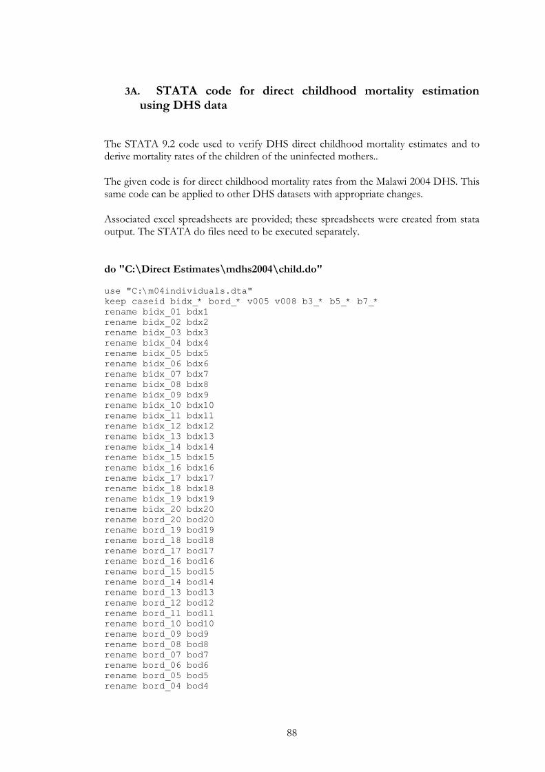
88
3A. STATA code for direct childhood mortality estimation using DHS data
The STATA 9.2 code used to verify DHS direct childhood mortality estimates and to derive mortality rates of the children of the uninfected mothers..
The given code is for direct childhood mortality rates from the Malawi 2004 DHS. This same code can be applied to other DHS datasets with appropriate changes.
Associated excel spreadsheets are provided; these spreadsheets were created from stata output. The STATA do files need to be executed separately.
do "C:\Direct Estimates\mdhs2004\child.do"
use "C:\m04individuals.dta"
keep caseid bidx_* bord_* v005 v008 b3_* b5_* b7_*
rename bidx_01 bdx1
rename bidx_02 bdx2
rename bidx_03 bdx3
rename bidx_04 bdx4
rename bidx_05 bdx5
rename bidx_06 bdx6
rename bidx_07 bdx7
rename bidx_08 bdx8
rename bidx_09 bdx9
rename bidx_10 bdx10
rename bidx_11 bdx11
rename bidx_12 bdx12
rename bidx_13 bdx13
rename bidx_14 bdx14
rename bidx_15 bdx15
rename bidx_16 bdx16
rename bidx_17 bdx17
rename bidx_18 bdx18
rename bidx_19 bdx19
rename bidx_20 bdx20
rename bord_20 bod20
rename bord_19 bod19
rename bord_18 bod18
rename bord_17 bod17
rename bord_16 bod16
rename bord_15 bod15
rename bord_14 bod14
rename bord_13 bod13
rename bord_12 bod12
rename bord_11 bod11
rename bord_10 bod10
rename bord_09 bod9
rename bord_08 bod8
rename bord_07 bod7
rename bord_06 bod6
rename bord_05 bod5
rename bord_04 bod4

89
rename bord_03 bod3
rename bord_02 bod2
rename bord_01 bod1
rename b3_01 b31
rename b3_02 b32
rename b3_03 b33
rename b3_04 b34
rename b3_05 b35
rename b3_06 b36
rename b3_07 b37
rename b3_08 b38
rename b3_09 b39
rename b3_10 b310
rename b3_11 b311
rename b3_12 b312
rename b3_13 b313
rename b3_14 b314
rename b3_15 b315
rename b3_16 b316
rename b3_17 b317
rename b3_18 b318
rename b3_19 b319
rename b3_20 b320
rename b5_01 b51
rename b5_02 b52
rename b5_03 b53
rename b5_04 b54
rename b5_05 b55
rename b5_06 b56
rename b5_07 b57
rename b5_08 b58
rename b5_09 b59
rename b5_10 b510
rename b5_11 b511
rename b5_12 b512
rename b5_13 b513
rename b5_14 b514
rename b5_15 b515
rename b5_16 b516
rename b5_17 b517
rename b5_18 b518
rename b5_19 b519
rename b5_20 b520
rename b7_01 b71
rename b7_02 b72
rename b7_03 b73
rename b7_04 b74
rename b7_05 b75
rename b7_06 b76
rename b7_07 b77
rename b7_08 b78
rename b7_09 b79
rename b7_10 b710
rename b7_11 b711
rename b7_12 b712
rename b7_13 b713
rename b7_14 b714
rename b7_15 b715
rename b7_16 b716
rename b7_17 b717
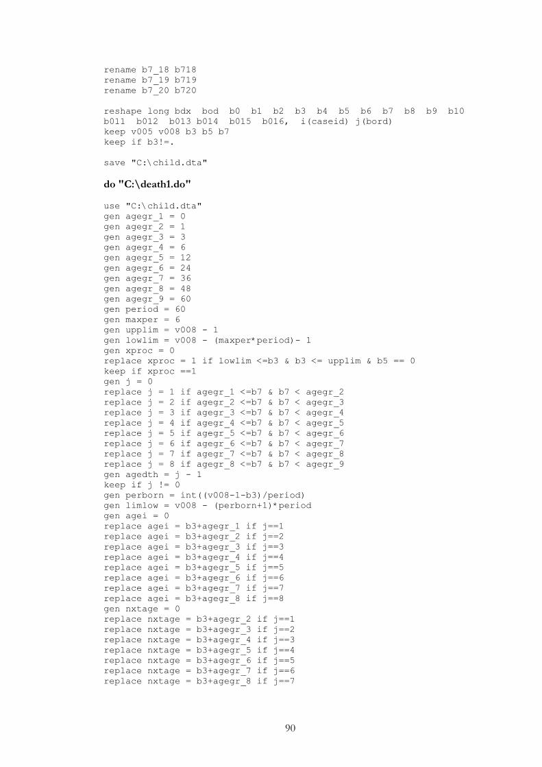
90
rename b7_18 b718
rename b7_19 b719
rename b7_20 b720
reshape long bdx bod b0 b1 b2 b3 b4 b5 b6 b7 b8 b9 b10
b011 b012 b013 b014 b015 b016, i(caseid) j(bord)
keep v005 v008 b3 b5 b7
keep if b3!=.
save "C:\child.dta"
do "C:\death1.do"
use "C:\child.dta"
gen agegr_1 = 0
gen agegr_2 = 1
gen agegr_3 = 3
gen agegr_4 = 6
gen agegr_5 = 12
gen agegr_6 = 24
gen agegr_7 = 36
gen agegr_8 = 48
gen agegr_9 = 60
gen period = 60
gen maxper = 6
gen upplim = v008 - 1
gen lowlim = v008 - (maxper*period)- 1
gen xproc = 0
replace xproc = 1 if lowlim <=b3 & b3 <= upplim & b5 == 0
keep if xproc ==1
gen j = 0
replace j = 1 if agegr_1 <=b7 & b7 < agegr_2
replace j = 2 if agegr_2 <=b7 & b7 < agegr_3
replace j = 3 if agegr_3 <=b7 & b7 < agegr_4
replace j = 4 if agegr_4 <=b7 & b7 < agegr_5
replace j = 5 if agegr_5 <=b7 & b7 < agegr_6
replace j = 6 if agegr_6 <=b7 & b7 < agegr_7
replace j = 7 if agegr_7 <=b7 & b7 < agegr_8
replace j = 8 if agegr_8 <=b7 & b7 < agegr_9
gen agedth = j - 1
keep if j != 0
gen perborn = int((v008-1-b3)/period)
gen limlow = v008 - (perborn+1)*period
gen agei = 0
replace agei = b3+agegr_1 if j==1
replace agei = b3+agegr_2 if j==2
replace agei = b3+agegr_3 if j==3
replace agei = b3+agegr_4 if j==4
replace agei = b3+agegr_5 if j==5
replace agei = b3+agegr_6 if j==6
replace agei = b3+agegr_7 if j==7
replace agei = b3+agegr_8 if j==8
gen nxtage = 0
replace nxtage = b3+agegr_2 if j==1
replace nxtage = b3+agegr_3 if j==2
replace nxtage = b3+agegr_4 if j==3
replace nxtage = b3+agegr_5 if j==4
replace nxtage = b3+agegr_6 if j==5
replace nxtage = b3+agegr_7 if j==6
replace nxtage = b3+agegr_8 if j==7
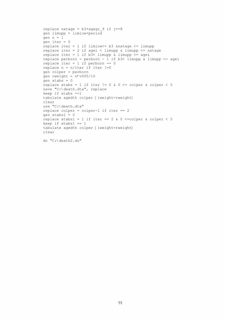
91
replace nxtage = b3+agegr_9 if j==8
gen limupp = limlow+period
gen n = 1
gen iter = 0
replace iter = 1 if limlow<= b3 &nxtage <= limupp
replace iter = 2 if agei < limupp & limupp <= nxtage
replace iter = 1 if b3< limupp & limupp <= agei
replace perborn = perborn - 1 if b3< limupp & limupp <= agei
replace iter = 1 if perborn == 0
replace n = n/iter if iter !=0
gen colper = perborn
gen rweight = n*v005/10
gen xtabs = 0
replace xtabs = 1 if iter != 0 & 0 <= colper & colper < 5
save "C:\death.dta", replace
keep if xtabs ==1
tabulate agedth colper [iweight=rweight]
clear
use "C:\death.dta"
replace colper = colper-1 if iter == 2
gen xtabs1 = 0
replace xtabs1 = 1 if iter == 2 & 0 <=colper & colper < 5
keep if xtabs1 == 1
tabulate agedth colper [iweight=rweight]
clear
do "C:\death2.do"
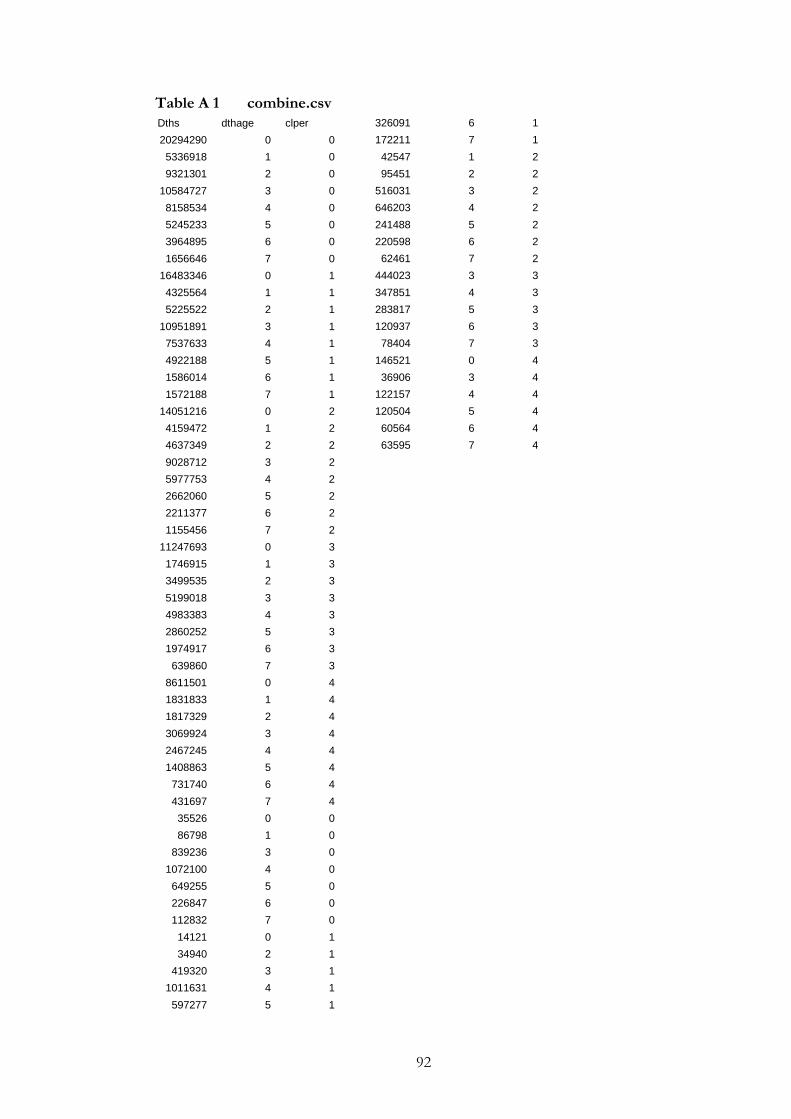
92
Table A 1 combine.csv
326091 6 1
172211 7 1
42547 1 2
95451 2 2
516031 3 2
646203 4 2
241488 5 2
220598 6 2
62461 7 2
444023 3 3
347851 4 3
283817 5 3
120937 6 3
78404 7 3
146521 0 4
36906 3 4
122157 4 4
120504 5 4
60564 6 4
63595 7 4
Dths dthage clper
20294290 0 0
5336918 1 0
9321301 2 0
10584727 3 0
8158534 4 0
5245233 5 0
3964895 6 0
1656646 7 0
16483346 0 1
4325564 1 1
5225522 2 1
10951891 3 1
7537633 4 1
4922188 5 1
1586014 6 1
1572188 7 1
14051216 0 2
4159472 1 2
4637349 2 2
9028712 3 2
5977753 4 2
2662060 5 2
2211377 6 2
1155456 7 2
11247693 0 3
1746915 1 3
3499535 2 3
5199018 3 3
4983383 4 3
2860252 5 3
1974917 6 3
639860 7 3
8611501 0 4
1831833 1 4
1817329 2 4
3069924 3 4
2467245 4 4
1408863 5 4
731740 6 4
431697 7 4
35526 0 0
86798 1 0
839236 3 0
1072100 4 0
649255 5 0
226847 6 0
112832 7 0
14121 0 1
34940 2 1
419320 3 1
1011631 4 1
597277 5 1
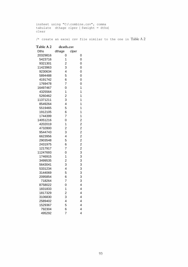
93
insheet using "C:\combine.csv", comma
tabulate dthage clper [fweight = dths]
clear
/* create an excel csv file similar to the one in Table A 2
Table A 2 death.csv Dths dthage clper
20329816 0 0
5423716 1 0
9321301 2 0
11423963 3 0
9230634 4 0
5894488 5 0
4191742 6 0
1769478 7 0
16497467 0 1
4325564 1 1
5260462 2 1
11371211 3 1
8549264 4 1
5519465 5 1
1912105 6 1
1744399 7 1
14051216 0 2
4202019 1 2
4732800 2 2
9544743 3 2
6623956 4 2
2903548 5 2
2431975 6 2
1217917 7 2
11247693 0 3
1746915 1 3
3499535 2 3
5643041 3 3
5331234 4 3
3144069 5 3
2095854 6 3
718264 7 3
8758022 0 4
1831833 1 4
1817329 2 4
3106830 3 4
2589402 4 4
1529367 5 4
792304 6 4
495292 7 4
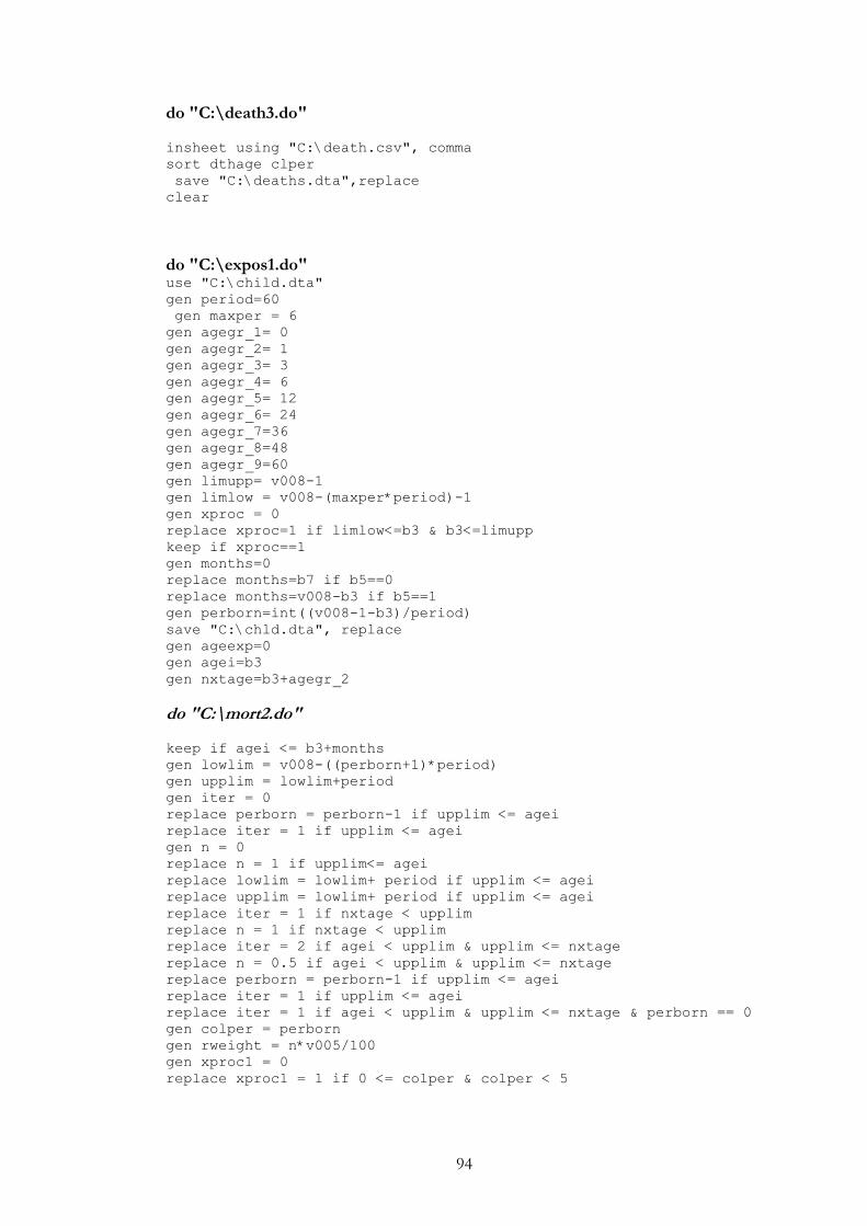
94
do "C:\death3.do"
insheet using "C:\death.csv", comma
sort dthage clper
save "C:\deaths.dta",replace
clear
do "C:\expos1.do" use "C:\child.dta"
gen period=60
gen maxper = 6
gen agegr_1= 0
gen agegr_2= 1
gen agegr_3= 3
gen agegr_4= 6
gen agegr_5= 12
gen agegr_6= 24
gen agegr_7=36
gen agegr_8=48
gen agegr_9=60
gen limupp= v008-1
gen limlow = v008-(maxper*period)-1
gen xproc = 0
replace xproc=1 if limlow<=b3 & b3<=limupp
keep if xproc==1
gen months=0
replace months=b7 if b5==0
replace months=v008-b3 if b5==1
gen perborn=int((v008-1-b3)/period)
save "C:\chld.dta", replace
gen ageexp=0
gen agei=b3
gen nxtage=b3+agegr_2
do "C:\mort2.do"
keep if agei <= b3+months
gen lowlim = v008-((perborn+1)*period)
gen upplim = lowlim+period
gen iter = 0
replace perborn = perborn-1 if upplim <= agei
replace iter = 1 if upplim <= agei
gen n = 0
replace n = 1 if upplim<= agei
replace lowlim = lowlim+ period if upplim <= agei
replace upplim = lowlim+ period if upplim <= agei
replace iter = 1 if nxtage < upplim
replace n = 1 if nxtage < upplim
replace iter = 2 if agei < upplim & upplim <= nxtage
replace n = 0.5 if agei < upplim & upplim <= nxtage
replace perborn = perborn-1 if upplim <= agei
replace iter = 1 if upplim <= agei
replace iter = 1 if agei < upplim & upplim <= nxtage & perborn == 0
gen colper = perborn
gen rweight = n*v005/100
gen xproc1 = 0
replace xproc1 = 1 if 0 <= colper & colper < 5
95
do "C:\mort3.do"
save "C:\mort2.dta", replace
keep if xproc1 == 1
tabulate ageexp colper [iweight=rweight]
clear
use "C:\mort2.dta"
gen colper1 = colper - 1
gen xproc2 = 0
replace xproc2 = 1 if 0 <= colper1 & colper1 <= 4 & iter == 2
keep if xproc2 == 1
tabulate ageexp colper1 [iweight=rweight]
clear
use "C:\chld.dta"
gen ageexp=1
gen agei=b3+agegr_2
gen nxtage=b3+agegr_3
do "C:\mort2.do" do "C:\mort3.do"
clear
use "C:\chld.dta"
gen ageexp=2
gen agei=b3+agegr_3
gen nxtage=b3+agegr_4
do "C:\mort2.do" do "C:\mort3.do"
clear
use "C:\chld.dta"
gen ageexp=3
gen agei=b3+agegr_4
gen nxtage=b3+agegr_5
do "C:\mort2.do"
do "C:\mort3.do"
clear
use "C:\chld.dta"
gen ageexp=4
gen agei=b3+agegr_5
gen nxtage=b3+agegr_6
do "C:\mort2.do"
do "C:\mort3.do"
clear
use "C:\chld.dta"
gen ageexp=5
gen agei=b3+agegr_6
gen nxtage = b3+agegr_7
do "C:\mort2.do" do "C:\mort3.do"
96
clear
use "C:\chld.dta"
gen ageexp=6
gen agei=b3+agegr_7
gen nxtage=b3+agegr_8
do "C:\mort2.do" do "C:\mort3.do"
clear
use "C:\chld.dta"
gen ageexp=7
gen agei=b3+agegr_8
gen nxtage=b3+agegr_9
do "C:\mort2.do" do "C:\mort3.do" clear
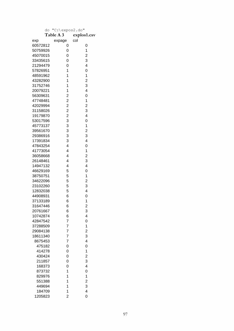
97
do "C:\expos2.do"
Table A 3 explos1.csv
exp expage col
60572812 0 0
50759926 0 1
45070015 0 2
33435615 0 3
21294479 0 4
57826951 1 0
48591962 1 1
43282900 1 2
31752746 1 3
20079221 1 4
56309631 2 0
47748481 2 1
42029994 2 2
31158026 2 3
19179870 2 4
53017596 3 0
45773137 3 1
39561670 3 2
29386916 3 3
17391834 3 4
47843254 4 0
41773054 4 1
36058668 4 2
26148461 4 3
14947132 4 4
46629169 5 0
38750751 5 1
34622096 5 2
23102260 5 3
12832038 5 4
44908931 6 0
37133189 6 1
31647446 6 2
20761667 6 3
10742874 6 4
42847542 7 0
37288509 7 1
29084138 7 2
18611340 7 3
8675453 7 4
475182 0 0
414278 0 1
430424 0 2
211857 0 3
168373 0 4
873732 1 0
829976 1 1
551388 1 2
449694 1 3
184709 1 4
1205823 2 0
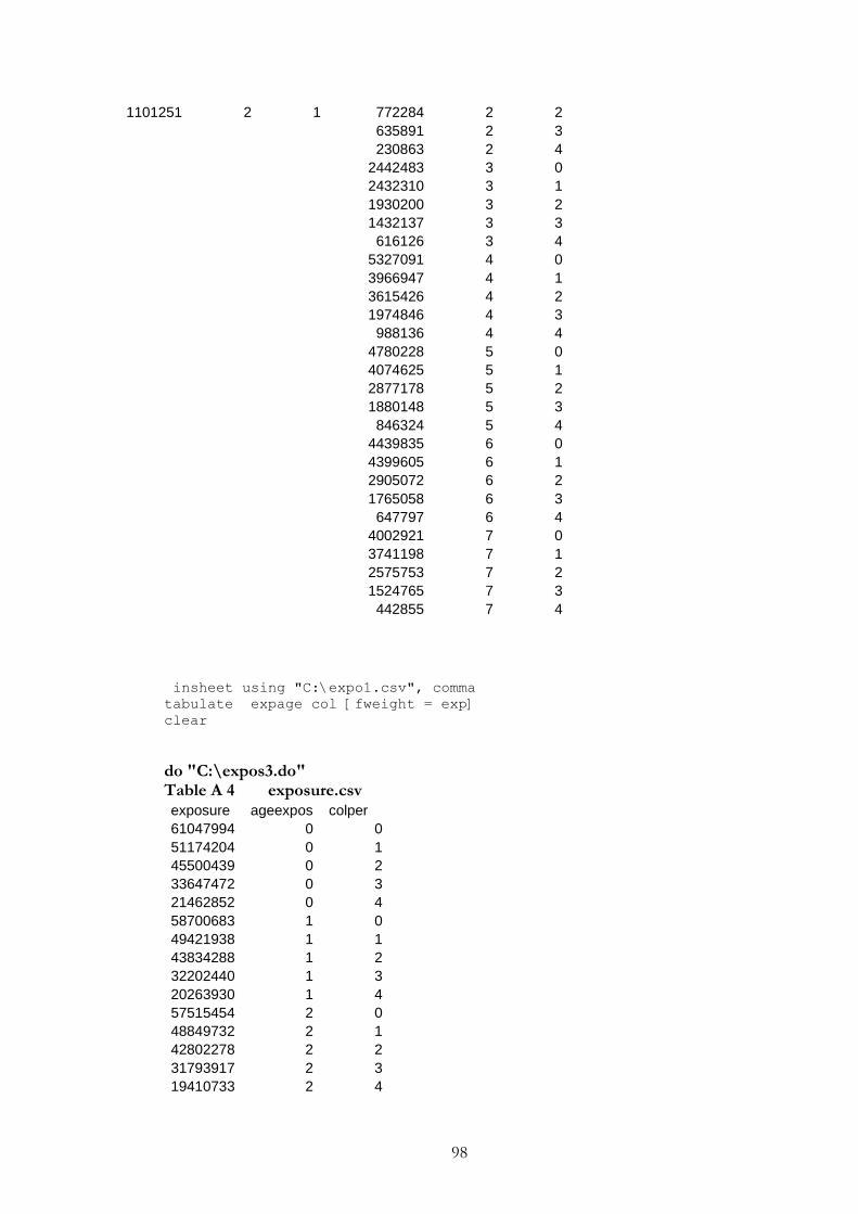
98
772284 2 2
635891 2 3
230863 2 4
2442483 3 0
2432310 3 1
1930200 3 2
1432137 3 3
616126 3 4
5327091 4 0
3966947 4 1
3615426 4 2
1974846 4 3
988136 4 4
4780228 5 0
4074625 5 1
2877178 5 2
1880148 5 3
846324 5 4
4439835 6 0
4399605 6 1
2905072 6 2
1765058 6 3
647797 6 4
4002921 7 0
3741198 7 1
2575753 7 2
1524765 7 3
442855 7 4
insheet using "C:\expo1.csv", comma
tabulate expage col [fweight = exp]
clear
do "C:\expos3.do" Table A 4 exposure.csv exposure ageexpos colper
61047994 0 0
51174204 0 1
45500439 0 2
33647472 0 3
21462852 0 4
58700683 1 0
49421938 1 1
43834288 1 2
32202440 1 3
20263930 1 4
57515454 2 0
48849732 2 1
42802278 2 2
31793917 2 3
19410733 2 4
1101251 2 1
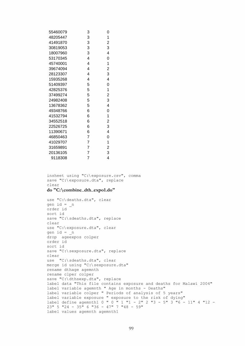
99
55460079 3 0
48205447 3 1
41491870 3 2
30819053 3 3
18007960 3 4
53170345 4 0
45740001 4 1
39674094 4 2
28123307 4 3
15935268 4 4
51409397 5 0
42825376 5 1
37499274 5 2
24982408 5 3
13678362 5 4
49348766 6 0
41532794 6 1
34552518 6 2
22526725 6 3
11390671 6 4
46850463 7 0
41029707 7 1
31659891 7 2
20136105 7 3
9118308 7 4
insheet using "C:\exposure.csv", comma
save "C:\exposure.dta", replace
clear
do "C:\combine_dth_expo1.do"
use "C:\deaths.dta", clear
gen id = _n
order id
sort id
save "C:\sdeaths.dta", replace
clear
use "C:\exposure.dta", clear
gen id = _n
drop ageexpos colper
order id
sort id
save "C:\sexposure.dta", replace
clear
use "C:\sdeaths.dta", clear
merge id using "C:\sexposure.dta"
rename dthage agemnth
rename clper colper
save "C:\dthsexp.dta", replace
label data "This file contains exposure and deaths for Malawi 2004"
label variable agemnth " Age in months - Deaths"
label variable colper " Periods of analysis of 5 years"
label variable exposure " exposure to the risk of dying"
label define agemnth1 0 " 0 " 1 "1 - 2" 2 "3 - 5" 3 "6 - 11" 4 "12 -
23" 5 "24 - 35" 6 "36 - 47" 7 "48 - 59"
label values agemnth agemnth1
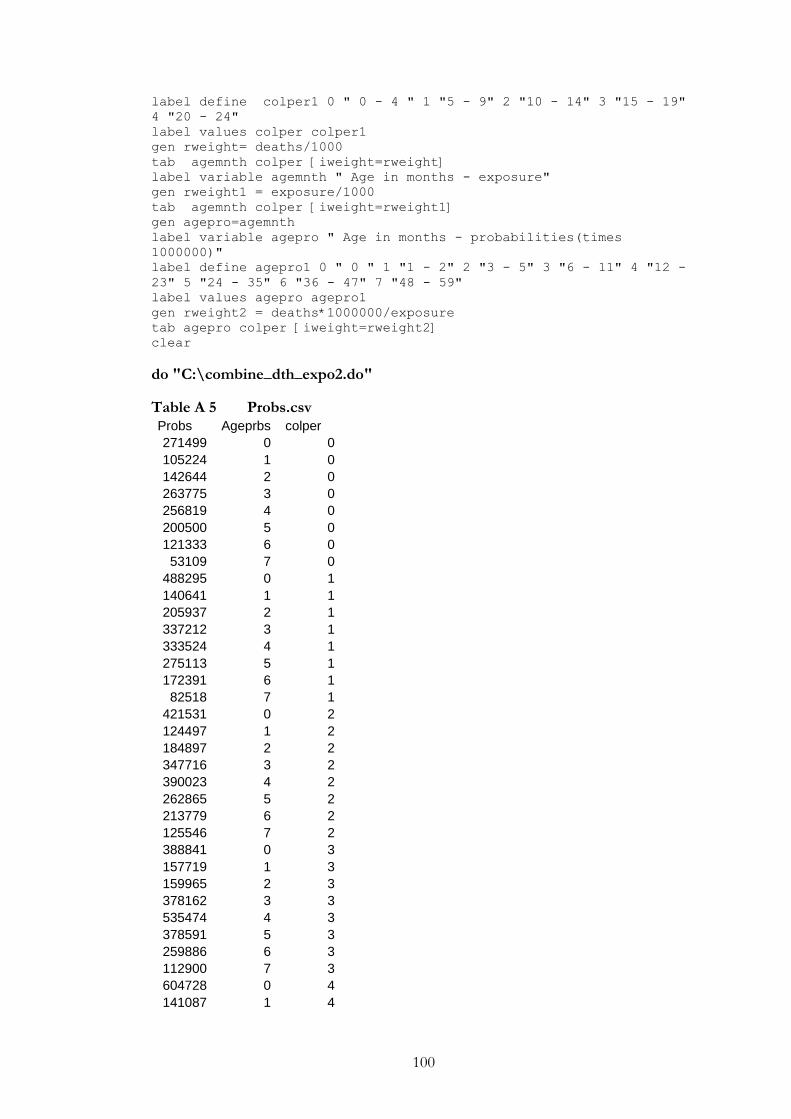
100
label define colper1 0 " 0 - 4 " 1 "5 - 9" 2 "10 - 14" 3 "15 - 19"
4 "20 - 24"
label values colper colper1
gen rweight= deaths/1000
tab agemnth colper [iweight=rweight]
label variable agemnth " Age in months - exposure"
gen rweight1 = exposure/1000
tab agemnth colper [iweight=rweight1]
gen agepro=agemnth
label variable agepro " Age in months - probabilities(times
1000000)"
label define agepro1 0 " 0 " 1 "1 - 2" 2 "3 - 5" 3 "6 - 11" 4 "12 -
23" 5 "24 - 35" 6 "36 - 47" 7 "48 - 59"
label values agepro agepro1
gen rweight2 = deaths*1000000/exposure
tab agepro colper [iweight=rweight2]
clear
do "C:\combine_dth_expo2.do"
Table A 5 Probs.csv Probs Ageprbs colper
271499 0 0
105224 1 0
142644 2 0
263775 3 0
256819 4 0
200500 5 0
121333 6 0
53109 7 0
488295 0 1
140641 1 1
205937 2 1
337212 3 1
333524 4 1
275113 5 1
172391 6 1
82518 7 1
421531 0 2
124497 1 2
184897 2 2
347716 3 2
390023 4 2
262865 5 2
213779 6 2
125546 7 2
388841 0 3
157719 1 3
159965 2 3
378162 3 3
535474 4 3
378591 5 3
259886 6 3
112900 7 3
604728 0 4
141087 1 4
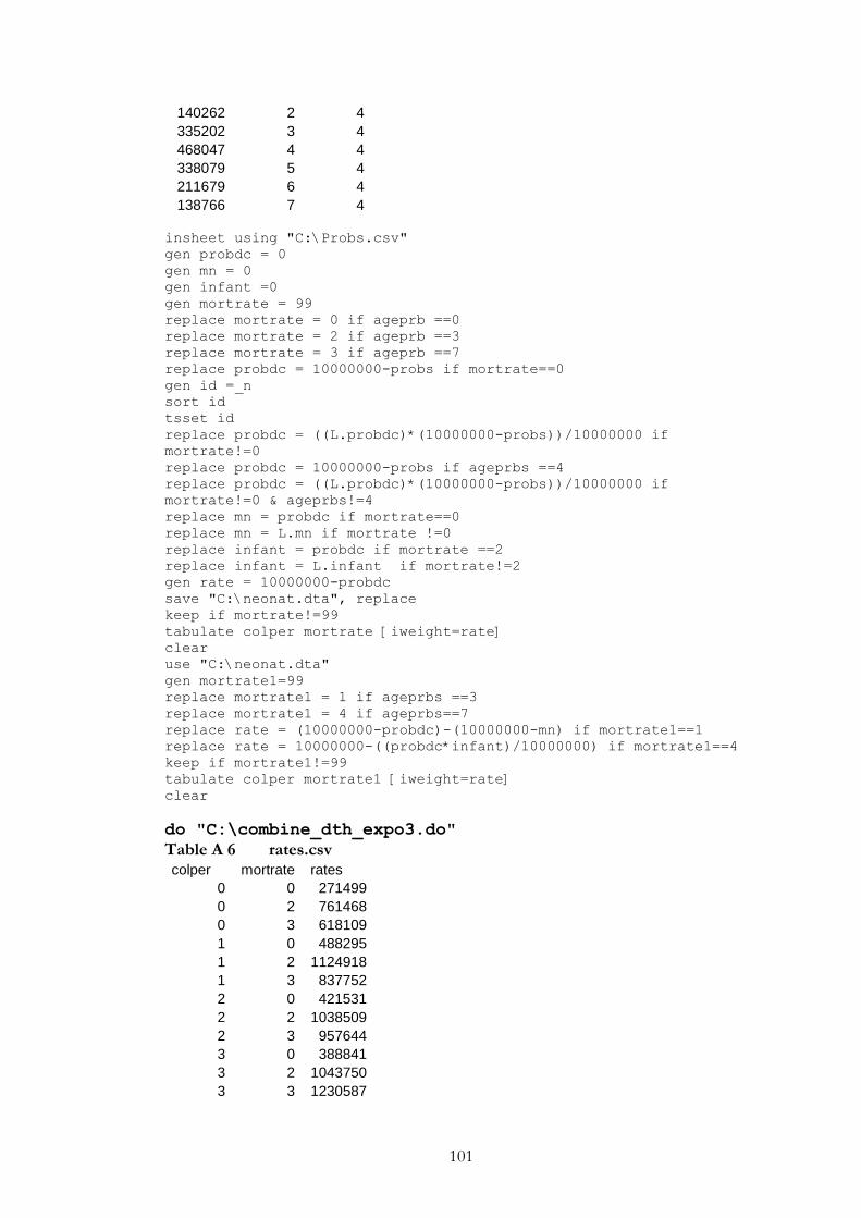
101
140262 2 4
335202 3 4
468047 4 4
338079 5 4
211679 6 4
138766 7 4
insheet using "C:\Probs.csv"
gen probdc = 0
gen mn = 0
gen infant =0
gen mortrate = 99
replace mortrate = 0 if ageprb ==0
replace mortrate = 2 if ageprb ==3
replace mortrate = 3 if ageprb ==7
replace probdc = 10000000-probs if mortrate==0
gen id =_n
sort id
tsset id
replace probdc = ((L.probdc)*(10000000-probs))/10000000 if
mortrate!=0
replace probdc = 10000000-probs if ageprbs ==4
replace probdc = ((L.probdc)*(10000000-probs))/10000000 if
mortrate!=0 & ageprbs!=4
replace mn = probdc if mortrate==0
replace mn = L.mn if mortrate !=0
replace infant = probdc if mortrate ==2
replace infant = L.infant if mortrate!=2
gen rate = 10000000-probdc
save "C:\neonat.dta", replace
keep if mortrate!=99
tabulate colper mortrate [iweight=rate]
clear
use "C:\neonat.dta"
gen mortrate1=99
replace mortrate1 = 1 if ageprbs ==3
replace mortrate1 = 4 if ageprbs==7
replace rate = (10000000-probdc)-(10000000-mn) if mortrate1==1
replace rate = 10000000-((probdc*infant)/10000000) if mortrate1==4
keep if mortrate1!=99
tabulate colper mortrate1 [iweight=rate]
clear
do "C:\combine_dth_expo3.do"
Table A 6 rates.csv colper mortrate rates
0 0 271499
0 2 761468
0 3 618109
1 0 488295
1 2 1124918
1 3 837752
2 0 421531
2 2 1038509
2 3 957644
3 0 388841
3 2 1043750
3 3 1230587
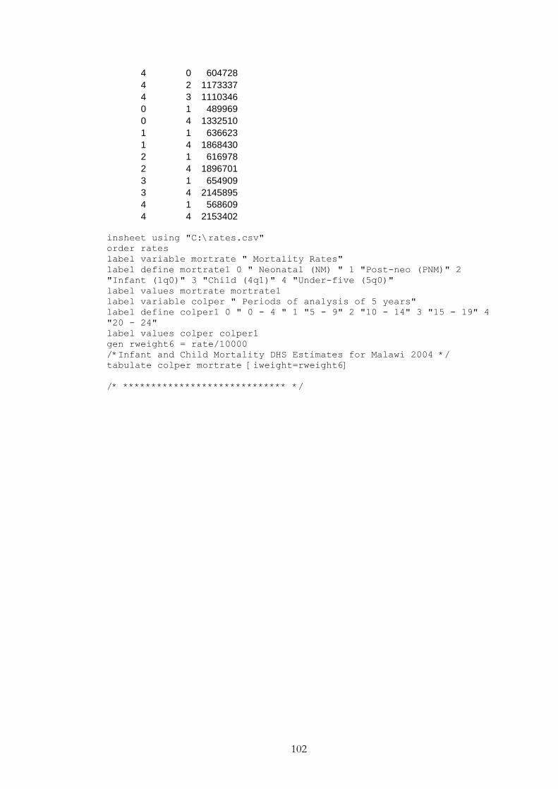
102
4 0 604728
4 2 1173337
4 3 1110346
0 1 489969
0 4 1332510
1 1 636623
1 4 1868430
2 1 616978
2 4 1896701
3 1 654909
3 4 2145895
4 1 568609
4 4 2153402
insheet using "C:\rates.csv"
order rates
label variable mortrate " Mortality Rates"
label define mortrate1 0 " Neonatal (NM) " 1 "Post-neo (PNM)" 2
"Infant (1q0)" 3 "Child (4q1)" 4 "Under-five (5q0)"
label values mortrate mortrate1
label variable colper " Periods of analysis of 5 years"
label define colper1 0 " 0 - 4 " 1 "5 - 9" 2 "10 - 14" 3 "15 - 19" 4
"20 - 24"
label values colper colper1
gen rweight6 = rate/10000
/*Infant and Child Mortality DHS Estimates for Malawi 2004 */
tabulate colper mortrate [iweight=rweight6]
/* ***************************** */