IS/ISO 13373 - 1 : 2002

© BIS 2011

January 2011 Price Group 14

B U R E A U O F I N D I A N S T A N D A R D SMANAK BHAVAN, 9 BAHADUR SHAH ZAFAR MARG

NEW DELHI 110002

Hkkjrh; ekud

e'khuksa dh voLFkk ekWuhVfjax rFkk MkbXuksfLVd —oaQiu fLFkfr dh ekWuhVfjax

Hkkx 1 lkekU; fofèk;k¡

Indian StandardCONDITION MONITORING AND DIAGNOSTICS OF

MACHINES — VIBRATION CONDITION MONITORING

PART 1 GENERAL PROCEDURES

ICS 17.160

Mechanical Vibration and Shock Sectional Committee, MED 28

NATIONAL FOREWORD

This Indian Standard (Part 1) which is identical with ISO 13373-1 : 2002 ‘Condition monitoring anddiagnostics of machines — Vibration condition monitoring — Part 1: General procedures’ issued bythe International Organization for Standardization (ISO) was adopted by the Bureau of Indian Standardson the recommendation of the Mechanical Vibration and Shock Sectional Committee and approval ofthe Mechanical Engineering Division Council.

The text of ISO Standard has been approved as suitable for publication as an Indian Standard withoutdeviations. Certain conventions are, however, not identical to those used in Indian Standards. Attentionis particularly drawn to the following:

a) Wherever the words ‘International Standard’ appear referring to this standard, they should beread as ‘Indian Standard’.

b) Comma (,) has been used as a decimal marker, while in Indian Standards, the current practiceis to use a point (.) as the decimal marker.

In this adopted standard, reference appears to certain International Standards for which IndianStandards also exist. The corresponding Indian Standards which are to be substituted in their respectiveplaces, are listed below along with their degree of equivalence for the editions indicated:

International Standard Corresponding Indian Standard Degree of Equivalence

ISO 1925 : 2001 Mechanical vibration— Balancing — Vocabulary

ISO 2041 : 1990 Vibration and shock— Vocabulary

ISO 7919-1 : 1996 Mechanicalvibrat ion of non-reciprocatingmachines —Measurements onrotating shafts and evaluation criteria— Part 1: General guidelines

ISO 10816-1 : 1995 Mechanicalvibration — Evaluation of machinevibration by measurements on non-rotating parts — Part 1: Generalguidelines

IS/ISO 1925 : 2001 Mechanicalvibration — Balancing — Vocabulary

IS 11717 : 2000 Vocabulary onvibration and shock (first revision)

IS 14773 (Part 1) : 2000 Mechanicalvibrat ion of non-reciprocatingmachines — Measurements onrotat ing shafts and evaluat ioncriteria: Part 1 General guidelines

IS 14817 (Part 1) : 2000 Mechanicalvibration — Evaluation of machinevibration by measurements on non-rotat ing parts: Part 1 Generalguidelines

Identical

do

do

do

For the purpose of deciding whether a particular requirement of this standard is complied with, thefinal value, observed or calculated, expressing the result of a test or analysis, shall be rounded off inaccordance with IS 2 : 1960 ‘Rules for rounding off numerical values (revised)’. The number ofsignificant places retained in the rounded off value should be the same as that of the specified valuein this standard.

1 Scope

This part of ISO 13373 provides general guidelines for the measurement and data collection functions of machinery vibration for condition monitoring. It is intended to promote consistency of measurement procedures and practices, which usually concentrate on rotating machines.

Because of the diversity of approaches to condition monitoring, recommendations specific to a particular kind of monitoring programme will be addressed in additional parts of ISO 13373.

This part of ISO 13373 is a basic document which presents recommendations of a general nature, encompassing

measurement methods,

measurement parameters,

transducer selection,

transducer location,

transducer attachment,

data collection,

machine operating conditions,

vibration monitoring systems,

signal conditioning systems,

interfaces with data-processing systems,

continuous monitoring, and

periodic monitoring.

The vibratory conditions of a machine can be monitored by vibration measurements on the bearing or housing structure and/or by vibration measurements of the rotating elements of the machine. In addition, measurements can be continuous or non-continuous. This part of ISO 13373 provides guidance on the types of measurements recommended in both the continuous and the non-continuous modes.

It is emphasized that this part of ISO 13373 addresses only the procedures for vibration condition monitoring of machines. In many cases, the complete condition monitoring and diagnostics of a machine can also include other parameters, such as thermography, oil analysis, ferrography, process variations, temperatures and pressures. These non-vibratory parameters will be included in other International Standards.

PART 1 GENERAL PROCEDURES

MACHINES — VIBRATION CONDITION MONITORINGCONDITION MONITORING AND DIAGNOSTICS OF

Indian Standard

IS/ISO 13373 - 1 : 2002

1

2

This part of ISO 13373 covers rotating machines. However, many of the procedures included can be applied to other types of machines, for example reciprocating machines.

2 Normative references

The following normative documents contain provisions which, through reference in this text, constitute provisions of this part of ISO 13373. For dated references, subsequent amendments to, or revisions of, any of these publications do not apply. However, parties to agreements based on this part of ISO 13373 are encouraged to investigate the possibility of applying the most recent editions of the normative documents indicated below. For undated references, the latest edition of the normative document referred to applies. Members of ISO and IEC maintain registers of currently valid International Standards.

ISO 1925, Mechanical vibration — Balancing — Vocabulary

ISO 2041, Vibration and shock — Vocabulary

ISO 7919-1, Mechanical vibration of non-reciprocating machines — Measurements on rotating shafts and evaluation criteria — Part 1: General guidelines

ISO 10816-1, Mechanical vibration — Evaluation of machine vibration by measurements on non-rotating parts — Part 1: General guidelines

3 Terms and definitions

For the purposes of this part of ISO 13373, the terms and definitions given in ISO 1925 and ISO 2041 apply.

4 Vibration condition monitoring

4.1 General

Vibration monitoring is conducted to assist in the evaluation of the “health” of the machine during sustained operation. Depending on the machine type and the critical components to be monitored, one or more measurement parameters, and a suitable monitoring system, have to be selected. The objective of such a programme is to recognize an “unhealthy” condition in sufficient time to take remedial action before certain defects in the machine parts significantly decrease equipment operation or projected machine life, or fail completely, thereby establishing a cost-effective maintenance plan.

Several types of condition monitoring systems are described below; depending on the machine, the machine’s condition and other factors, any one of the systems, or combinations thereof, may be selected.

4.2 Types of vibration condition monitoring systems

4.2.1 General

Condition monitoring systems take many forms. They utilize permanently installed, semi-permanent or portable measuring equipment.

A decision to select the appropriate measuring system depends upon a number of factors, such as

criticality of the machine operation,

cost of machine down-time,

cost of catastrophic failure,

cost of the machine,

IS/ISO 13373 - 1 : 2002

rate of progress of the failure mode,

accessibility for repair/maintenance (e.g. in nuclear plants or other remote locations),

accessibility of the appropriate measurement positions,

quality of the measurement/diagnostic system,

operational modes of the machine (e.g. speed, power),

cost of the monitoring system,

safety, and

environmental impacts.

4.2.2 Permanently installed systems

This type of system is one in which the transducers, signal conditioners, data-processing and data-storage equipment are permanently installed. Data may be collected either continuously or periodically. The application of permanently installed systems is usually limited to costly and critical machinery or to machines with complex monitoring tasks. Figure 1 shows a typical permanently installed on-line system.

4.2.3 Semi-permanent systems

The semi-permanent system is a cross between the permanent and portable systems. In this type of system the transducers are generally permanently installed, whereas the electronic data-acquisition components are intermittently connected.

4.2.4 Portable monitoring systems

A portable monitoring system performs similar functions as the “continuous” on-line system, but it is less elaborate and normally less expensive. With this arrangement, the data are recorded periodically either automatically or manually, with a portable data collector. This type of system is shown in Figure 2.

More commonly, portable monitoring systems are used to record manually measurements at preselected locations on the machine at periodic intervals (weekly, monthly, etc.). The data are usually entered and stored locally on a portable data collector. A preliminary cursory analysis can be done immediately; however, for more in-depth processing and analysis, the data is downloaded to a personal computer that has the appropriate software.

4.3 Data collection

4.3.1 General

Data may be collected on a continuous or periodic basis; and the data analysis may be driven by events or by intervals.

4.3.2 Continuous data collection

A continuous data-collection system is one in which vibration transducers are installed permanently at key locations on the machine (as shown in Figure 1), and in which the vibration measurements are usually recorded and stored continuously, during operation of the machine. It can include automatic vibration monitoring systems with multiplex connections provided that the multiplexing rate is sufficiently rapid so that no significant data or trends are lost. The data may be processed to provide either broadband or spectral information which can be compared to previously acquired data. By setting “alert limits” on the stored data it is possible to inform the operator that the vibratory pattern of the machine has changed (the magnitude has either increased or decreased), and therefore diagnostic procedures are recommended.

IS/ISO 13373 - 1 : 2002

3

4

Key

1 Driver 6 Radial 2 Shaft displacement probes (typical) 7 Axial 3 Phase reference 8 Printer 4 Transducers on stationary bearing structure (typical) 9 Computer with data storage 5 Driven process machinery 10 Signal conditioner

NOTE This figure shows one typical arrangement. Alternative systems are permissible (e.g. microprocessor-based systems often have integral signal conditioning which may be carried out after the A/D conversion).

Figure 1 — Typical permanently installed on-line vibration condition monitoring system

Key

1 Driver 7 Printer 2 Data points (typical) 8 Computer with data storage 3 Phase reference 9 Computer link 4 Driven process machinery 10 Portable data logger 5 Radial 11 Transducer 6 Axial

Figure 2 — Typical portable monitoring system

IS/ISO 13373 - 1 : 2002

A continuous data-collection system can be installed at the machine site for direct use by the machine operating crew, or it can be installed at remote sites with data transmitted to a central data analysis centre. The obvious advantage of a “continuous” system is the availability of on-line machine condition in real time.

In an automatic system, permanent vibration transducers are installed on the machine in much the same manner as with the continuous monitoring system. The system is programmed to record and store data automatically. The last data are compared with the previously stored data in order to determine whether an ALARM condition exists.

A decision to select a continuous data-collection system should be taken after consideration of the factors listed in 4.2.1.

4.3.3 Periodic data collection

Periodic data collection can be done with either permanent on-line or portable systems. On-line periodic systems may include automatic vibration monitoring systems with multiplexer connections. In this case all channels are cyclically scanned one after the other with respect to off-limit conditions. The measuring system is permanently in action but there are gaps in monitoring the individual measuring points, which are dependent on the number of channels monitored and the measuring period per channel. These systems are sometimes referred to as “scanning” or “intermittent” systems.

For machines for which permanent on-line systems cannot be justified, portable systems are usually used and they are in most cases suitable for periodic monitoring.

4.4 Condition monitoring programme

After selection of the equipment to be monitored, and determining the type of measurement system that is appropriate, it is recommended that a condition monitoring programme flowchart be developed. Figure 3 shows such a typical flowchart. However, since each plant and each system is unique, the data flow should be customized to provide the maximum benefits.

Clear descriptions of operating conditions, such as speed, load or temperature, should accompany any vibration data collected. As a minimum, such descriptions should include shaft speed (r/min) and machine load (power, flow, pressure, etc.) and any other operating parameter that can affect the measured vibration.

In general, during data acquisition it is strongly emphasized that the operating conditions should approximate the normal operating conditions of the machine as closely as possible, to ensure consistency and valid comparability of the data. When this is not possible, the characteristics of the machine must be well known in order to evaluate any differences in the data.

Since the procedure of condition monitoring includes the process of “trending”, which examines the rate at which vibration values change with operating time, it is especially important that the operating conditions during successive measurements remain the same, in order for such trending to be valid. For example, in the case of pumps, the vibration values can vary significantly between “normal” and “off-normal” operating loads. Thus, a change in vibration response due to a change in operating conditions could easily be incorrectly interpreted as a change due to an impending problem.

In addition, the time rate of data acquisition need not to be constant. As pointed out in 7.3, it depends on the current condition of the machine.

Data under other conditions may also need to be collected depending on the complexity of the machine and the purpose of the measurement. For example, where problems with unbalance, rubbing, shaft cracks or oil whirl are suspected, testing during transient operating conditions such as start-up and shut-down is recommended.

IS/ISO 13373 - 1 : 2002

5

6

Figure 3 — Vibration condition monitoring flowchart

IS/ISO 13373 - 1 : 2002

5 Measurements

5.1 General

This clause provides information on the types of measurements and the measurement quantities recommended for vibration condition monitoring. Annex B lists the typically required information to be recorded for each machine and measurement.

5.2 Types of measurements

5.2.1 General considerations

In general, there are three types of measurements that may be employed for machine vibration condition monitoring, as follows:

a) vibration measurements made on the non-rotating structure of the machine, such as the bearing housings, machine casing or machine base;

b) relative motion between the rotor and the stationary bearings or housing;

c) absolute vibratory motion of the rotating elements.

Vibration measurements on structures would normally use r.m.s. velocity often combined with r.m.s. displacement or acceleration (see ISO 10816-1). If the vibration is predominantly sinusoidal, vibratory displacement (zero-to-peak or peak-to-peak) may also be used.

For high-speed machines/gears and machines with anti-friction bearings, peak acceleration is often used for monitoring in combination with r.m.s. velocity. In addition, increasing use is being made of other more sophisticated techniques which enable greater use to be made of the information contained within the vibration signal.

Absolute and relative displacement of the rotating components are further defined by several different displacement quantities, each of which is now in widespread use and is defined in ISO 7919-1. These include

Smax, the maximum value of shaft displacement from the time-integrated zero mean position, and

Sp-p, the vibratory peak-to-peak displacement in the direction of measurement.

Each of these displacement quantities may be used for measurement of shaft vibration. However, the quantities shall be clearly identified so as to ensure correct interpretation of the measurements.

It should be noted that the ISO 7919 and ISO 10816 series address broadband measurements only. However, condition monitoring may include additional vibration measurements and analyses such as

spectral analysis,

filtering,

time wave forms and orbits,

vector analysis with magnitude and phase, and

analysis of the high-frequency vibration envelope.

IS/ISO 13373 - 1 : 2002

7

8

5.2.2 Transducer locations

The locations of transducers for the purposes of condition monitoring depend on the particular machine and the specific parameters to be measured. Before specifying “location”, it is first necessary to identify which parameters should be monitored, i.e.

the absolute vibration of the machine housing,

the vibratory motion of the rotor relative to the housing,

the position of the shaft relative to the housing during machine operation, and

the absolute motion of the shaft.

In general, the transducers should be located at or near the bearings. However, if experience is available for a particular type of machine and if such transducer locations are practical, it could be useful to locate transducers at other positions than the bearings, as follows:

a) at the positions which are most likely to provide maximum values of vibration (such as intermediate shaft mid-span of large gas turbine units);

b) at the positions where a small clearance exists between the static and rotating parts and rubbing may occur.

Whatever the plane chosen for the vibration measurement, transducers should be located at those angular positions which are most likely to provide early indications of wear or failure.

5.2.3 Transducer locations for typical machines

Annex A includes a table showing recommended locations for obtaining meaningful vibration data for various types of machines. These locations and directions provide for shaft measurements near the bearings.

5.2.4 Transducer orientation and identification

The locations of the transducers should be clearly marked and identified to ensure repeatability of location during successive measurements. It is important to establish a consistent naming convention for assets and measurement points. Annex D provides an example of a typical convention for transducer orientation and identification.

5.2.5 Measurements on non-rotating structures

The ISO 10816 series provides specific procedures and instrumentation for different classes of machinery and identifies r.m.s. vibration velocity (in millimetres per second) as the preferred evaluation parameter. Measurements may be made either directly by a velocity transducer or by an accelerometer with an integrating circuit.

Typical locations for these types of measurements for horizontal machines are on each bearing housing or pedestal as shown in Figure 4. For vertical machines, see Figure 5.

IS/ISO 13373 - 1 : 2002

X horizontal Y vertical Z axial

Figure 4 — Schematic diagram of typical transducer locations for vibration measurements on horizontal machines

IS/ISO 13373 - 1 : 2002

9

10

Figure 5 — Schematic diagram of typical transducer locations for vibration measurement on vertical machines

IS/ISO 13373 - 1 : 2002

5.2.6 Measurements on rotating shafts

5.2.6.1 General

As defined in ISO 7919-1, the preferred measurement quantity for the measurement of shaft vibration is displacement. The following subclauses describe various transducers and arrangements for shaft measurements. Also shown on the figures are references to local signal conditioning and data processing. A discussion of signal conditioning is given in 5.2.8.

NOTE Details of further signal processing and analysis and displaying of the data will be given in ISO 13373-2 which is at present under preparation.

5.2.6.2 Relative motion of shaft to housing

The ISO 7919 series provides specific procedures and instrumentation for the measurement of broadband vibratory displacements of rotating shafts for different classes of machinery.

The relative displacement is best measured by using two non-contacting transducers arranged to measure radial relative motion between the rotating shaft or element and the stationary element in the same transverse plane. Figure 6 provides a typical installation of such a non-contacting transducer system.

At each bearing, the transducers are normally mounted orthogonally in the bearing or as close to the bearing housing as possible. There could be occasions, such as on flexible shaft machinery, where it would be advisable to mount the transducers at locations other than at the bearings.

In any event, the transducer locations shall be arranged such that they provide adequate sensitivity to the machine dynamic forces. Although the transducers may be placed at any angular position, it is common to locate them vertically and horizontally or at ± 45° from the vertical and horizontal, depending on ready access to the rotating shaft. A single transducer may be used if it is known to provide adequate information about the machine, however, some analysis techniques will then no longer be possible, such as orbit analysis and Smax.

Key

1 Local signal conditioners 2 To signal processing 3 Optional transducer orientations 4 Shaft 5 Non-contacting transducers

Figure 6 — Schematic diagram of relative motion measurement system using non-contacting transducers

IS/ISO 13373 - 1 : 2002

11

12

5.2.6.3 Absolute motion of shaft

Some types of machines, such as those having soft rotor support structures and/or flexible rotors, or machines operating near a rotor natural frequency, could require the measurement of absolute motion of the shaft.

Figures 7 and 8 provide examples of measurement systems for determining the absolute motion of the shaft. The preferred method is a combination of non-contacting and seismic transducers, as shown in Figure 7. Although the shaft riding transducer shown in Figure 8 may be used in some cases, it should be noted that this method has a limited frequency range and that the method will not provide the shaft radial position.

Key 1 Local signal conditioners 4 Shaft 2 Remote readout instrumentation 5 Non-contacting transducers 3 Optional output for instruments for recording 6 Seismic transducers alarm/trips and/or data analysis 7 Machine structure

Figure 7 — Schematic diagram of absolute/relative motion measurement system using a combination of non-contacting and seismic transducers

Key 1 Local signal conditioners 4 Shaft riders 2 To signal processing 5 Seismic transducers 3 Shaft 6 Machine structure

Figure 8 — Schematic diagram of absolute motion measurement system using shaft-rider mechanism with seismic transducers

IS/ISO 13373 - 1 : 2002

5.2.7 Torsional vibration

Routine monitoring of torsional vibration on rotating machines is currently uncommon. It may become more frequently used in the future, in particular for monitoring variable-frequency a.c. driven machines. It has typically been used at a limited number of power plants in the electrical power generation industry, to gain improved understanding of the severity of interactions of the torsional dynamics of large steam turbine generator sets and the electrical oscillations in the transmission network. This involves monitoring turbine generator shaft torsional response due to transient disturbances in the network (e.g. faults, short circuits), and continuously acting steady-state stimuli from the network (e.g. unbalanced transmission lines). The monitoring equipment to do this is very specialized and can be very expensive, and it requires linkage to a computer for data processing to convert mechanical information acquired at several positions on the turbine generator shaft to provide estimates of fatigue life expenditure at the most critical positions within the machine (see also clause C.3).

When torsional vibration measurements are required, they are usually made by measuring the oscillatory speed variations of the machine at selected transducer locations. Commonly used transducer systems are as follows.

Free-end mounted torsiograph which measures vibratory angular velocity. The vibratory velocity signal may be electronically integrated to provide a torsional displacement amplitude.

Free-end or mid-shaft toothed wheels in combination with an electromagnetic transducer mounted on the stationary structure. The transducer provides a signal of the instantaneous oscillatory speed of the target “toothed” wheel. This signal is usually conditioned to provide a torsional displacement signal.

Mid-shaft or free-end mounted disks with radial code markings in combination with optical transducers which measure the instantaneous speed and phase variations of the target lines. This signal is electronically conditioned to provide torsional displacement signals.

Strain gauges mounted on the shaft to measure directly the alternating component of torsional strain.

Laser systems.

Regardless of the type of measurement used, mathematical simulation is required to convert measurement information taken at a selected location to response estimates at other locations of interest. In general, the conversion of mechanical measurements to stress and fatigue responses is very complex, requiring sophisticated analytical procedures.

NOTE The hardware and software systems that have been used and the analysis of torsional vibration are well documented in the technical literature and will not be discussed in this part of ISO 13373.

5.2.8 Signal-conditioning systems

Signals derived from vibration transducers typically require some degree of conditioning to provide a useful measurement. Signal-conditioning functions may include conversion of the transducer output signal to a measurable quantity such as current or voltage, and processing of the signal into a suitable form for the measurement required.

Common examples of such condition processing are amplification/attenuation, filtering, scaling, d.c. offset and integration.

Depending on the complexity of the measurement system, the necessary signal-conditioning circuitry may be

an integral part of the transducer,

an integral part of the measurement instrument,

separate, self-contained instrumentation in the signal path between the transducer and the measurement instrument, or

a combination of the above.

IS/ISO 13373 - 1 : 2002

13

14

In simple systems, where signal-conditioning functions are built into the transducer or the measurement instrument (or both), the user may have little or no choice as to signal-conditioner settings. However, in more complex equipment with broader variability and more options in signal conditioning, care shall be taken to maintain accurate records of all settings so that subsequent measurements duplicate the original settings. Comparison of measurements taken at signal-conditioner settings which are not identical can lead to very serious errors in condition assessment, because ensuing changes in measured quantities may be incorrectly attributed to changes in machinery condition.

When external signal conditioning is applied between the transducer and the measurement instrument, it is essential to be aware of signal levels and instrument dynamic ranges in order to avoid introducing distortion into the measurement.

Additionally, the frequency response characteristics of the signal conditioner(s) shall be properly matched to the remaining instrumentation to obtain valid results.

NOTE Information on signal processing and analysis will be given in ISO 13373-2, which is at present under preparation.

5.3 Measurement quantities

5.3.1 General

Vibration may be quantified in the form of linear or angular displacement, velocity or acceleration. Except in special cases (discussed in other clauses of this part of ISO 13373), the recommended quantity for condition monitoring on stationary parts of machinery is vibration velocity. For monitoring the relative position and motion of rotating parts, displacement is recommended. Acceleration is the recommended measurement quantity for condition monitoring of rolling element bearings and gears, for example, as they may exhibit faults at high frequency. In any case a selection of the measurement quantity should be based largely on the anticipated frequency of excitation.

Shafts with fluid-film bearing supports may experience a d.c. or static shift of the shaft position when the machine is placed in operation from rest. Although this displacement is not directly a vibration component, as there is no motion after the initial positioning, it is a value provided by the vibration displacement transducers, and it should be recorded since it provides the base position from which to measure the shaft dynamic vibration behaviour of the machine.

5.3.2 Magnitude range

The magnitude range to be measured shall be selected on the basis of previous experience or the criteria applied for evaluation of the particular machine being monitored, covering the lowest to the highest anticipated amplitude. In the absence of previous experience, refer to the applicable International Standard (e.g. the ISO 7919 or ISO 10816 series) for the magnitude range recommended for velocity measurements.

Test equipment should be designed to ensure that its self-noise is at least 10 dB below, or one-third of, the lowest vibration value to be measured, while ensuring that the system can accommodate signals at least 10 dB higher than the largest expected signals.

5.3.3 Frequency range

For reliable condition monitoring, measuring equipment shall be capable of covering a wide frequency range in order to encompass not only shaft rotational frequencies and harmonics, but also frequencies due to other components, such as bearings, gears, seals, blades or vanes. The frequency range measured should be tailored to the specific machine(s) being monitored, if possible, but it should normally not be greater than the maximum transducer linear range.

The maximum transducer linear range is the range of frequencies and amplitudes for which the calibration sensitivity of the transducer is a constant, within the specified measurement accuracy. Refer to 5.4 for further definition of measurement accuracy.

The linear frequency range of the system should generally cover frequencies from 0,2 times the lowest rotational frequency to 3,5 times the highest excitation frequency of interest (generally not exceeding 10 kHz). Typically, the

IS/ISO 13373 - 1 : 2002

highest excitation frequency is the rotational frequency multiplied by the number of blades, gear teeth or vanes, etc., or it may be one of the rolling element bearing frequencies. For pumps, cavitation-excited vibration can also occur and be outside these ranges.

For mechanical suitability, 10 kHz is adequate. However, for diagnosing very high-frequency signals, as in the case of gears or rolling element bearings, the 10 kHz limit may be increased, even beyond the transducer manufacturer’s recommended linear operating range, as shown in Figure 9. In these instances, although the individual high-frequency signals may not be completely accurate in amplitude, the signals can provide valuable information.

NOTE More information regarding very-high-frequency analysis will be given in ISO 13373-2, which is at present under preparation.

5.3.4 Phase

The phase angle between two vibration sources is an important consideration when evaluating signals. Phase is a measure of the angular or time difference of one sinusoidal vibration signal to another, or of a vibration signal to a fixed reference. For the purposes of condition monitoring, phase lag is commonly used. A fixed transducer, capable of generating a signal when a reference point on the shaft passes, is used as the phase reference. The phase lag corresponds, for example, to the delay time between a reference point on the shaft and the maximum or zero crossing of the vibration signal. The phase reference may also be used for synchronous time averaging.

The physical location of the phase reference point, often called a trigger location, is arbitrary. However, a keyway in the shaft, if accessible, is recommended as the reference point. Lacking a keyway, any other discontinuity of the shaft that exists only once per revolution and can create a distinct signal, may be used as a permanent phase reference.

The most common use of phase measurement is in the determination and correction of unbalances. In addition, phase measurements may be used to include fault detection through the measurement of relative motion between machine components, thermal vectoring, verification of misalignment, rotor cracks, the determination of cross-coupling effects and the identification of machine resonance.

When measuring phase between two locations, it is important to use similar transducers and associated signal-conditioning equipment in order to avoid instrumentation phase errors. Otherwise, compensations shall be made for the differences.

5.4 Measurement accuracy and repeatability

An acceptable measurement under this procedure falls into two categories as shown in Figure 9.

Type 1 measurements will have an allowable tolerance of ± 5 % of the calibration sensitivity for the required amplitude and frequency range of the measurement.

Type 2 measurements will have an allowable tolerance of ± 10 % of the calibration sensitivity for the required amplitude and frequency range of the measurement.

Measurements with greater than 10 % variations in calibration sensitivity over the required amplitude and frequency ranges are not in accordance with this procedure, unless special precautions are taken to return them to within the required tolerances. Measurements made in accordance with this procedure should be stated as such using the appropriate Type 1 or Type 2 designation.

Of equal importance, or in some cases more important, is the repeatability of the data. Therefore, the data should be taken with the same instrumentation, means of attachment, sensitivities and calibrations. Otherwise, unless accurately known compensations can be made, comparisons and trending of the machine condition signals can be misleading.

It should also be noted that the response curve of Figure 9 is of a general shape. Each transducer type described below has distinct characteristics, and the actual response curve should be obtained for each transducer selected.

IS/ISO 13373 - 1 : 2002

15

16

1 Type 1 linear range 2 Type 2 linear range

Figure 9 — System frequency response

6 Transducers

6.1 Transducer types

There are two basic types of transducers for vibration condition monitoring, as follows:

a) seismic devices that are normally mounted on the machine structure and whose output is a measure of the absolute vibration of the structure;

b) relative displacement transducers that measure the vibratory displacement and the mean position between rotating and non-rotating elements of the machine.

There are some machinery measurements that require other types of transducers, such as strain gauges. However, their use for condition monitoring is less common.

6.2 Transducer selection

6.2.1 General considerations

The selection of appropriate transducers depends on the particular application. In general, the transducers for condition monitoring are

the accelerometer, whose output can be processed to yield any of the three parameters (acceleration, velocity and displacement),

IS/ISO 13373 - 1 : 2002

the velocity transducer, whose output can be integrated to yield displacement, and

the non-contacting probe, whose output is directly proportional to the relative displacement between the rotating and non-rotating elements of the machine.

Figure 10 includes selection guidelines for the three types of transducers and their dynamic ranges versus frequency. The ranges shown include the majority of applications for condition monitoring. Under special circumstances, individual transducer ranges may be extended, primarily for diagnostic purposes.

NOTE The values given below are typical examples. Specific transducers can have different, especially broader ranges.

1 Piezo-electric accelerometer 2 Eddy-current proximity probe 3 Electro-mechanical velocity transducer a To d.c.

Figure 10 — Dynamic range versus frequency range for the application of transducers typically used for machine condition monitoring

6.2.2 Accelerometers

6.2.2.1 General

An accelerometer is a seismic device that generates an output signal proportional to the mechanical vibratory acceleration of the body being measured. In general, accelerometers are mounted on the stationary (non-rotating) structure of the machine. Accelerometers are available with various mounted resonant frequencies, typically from 1 kHz upwards. In general it is recommended that the linear range of the mounted accelerometer covers the frequencies of interest. It is common to integrate the output of an accelerometer to provide a velocity signal. However, caution shall be exercised when double-integrating to provide displacement, especially at low frequencies.

IS/ISO 13373 - 1 : 2002

17

18

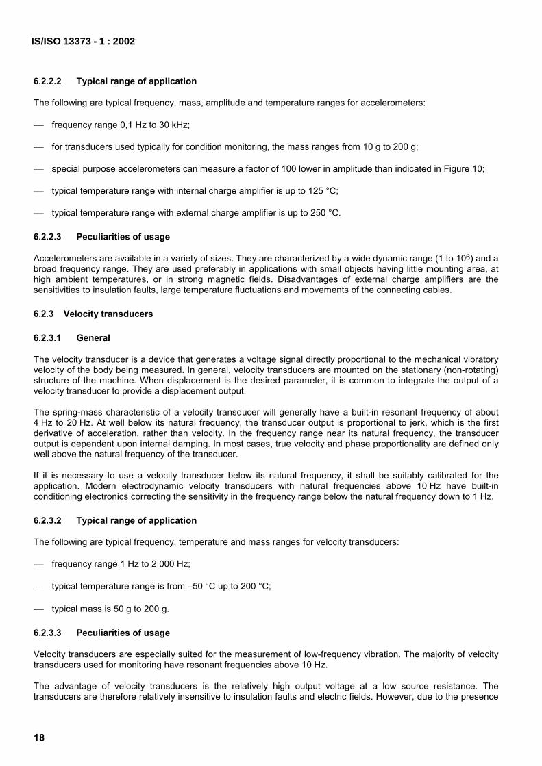
6.2.2.2 Typical range of application

The following are typical frequency, mass, amplitude and temperature ranges for accelerometers:

frequency range 0,1 Hz to 30 kHz;

for transducers used typically for condition monitoring, the mass ranges from 10 g to 200 g;

special purpose accelerometers can measure a factor of 100 lower in amplitude than indicated in Figure 10;

typical temperature range with internal charge amplifier is up to 125 °C;

typical temperature range with external charge amplifier is up to 250 °C.

6.2.2.3 Peculiarities of usage

Accelerometers are available in a variety of sizes. They are characterized by a wide dynamic range (1 to 106) and a broad frequency range. They are used preferably in applications with small objects having little mounting area, at high ambient temperatures, or in strong magnetic fields. Disadvantages of external charge amplifiers are the sensitivities to insulation faults, large temperature fluctuations and movements of the connecting cables.

6.2.3 Velocity transducers

6.2.3.1 General

The velocity transducer is a device that generates a voltage signal directly proportional to the mechanical vibratory velocity of the body being measured. In general, velocity transducers are mounted on the stationary (non-rotating) structure of the machine. When displacement is the desired parameter, it is common to integrate the output of a velocity transducer to provide a displacement output.

The spring-mass characteristic of a velocity transducer will generally have a built-in resonant frequency of about 4 Hz to 20 Hz. At well below its natural frequency, the transducer output is proportional to jerk, which is the first derivative of acceleration, rather than velocity. In the frequency range near its natural frequency, the transducer output is dependent upon internal damping. In most cases, true velocity and phase proportionality are defined only well above the natural frequency of the transducer.

If it is necessary to use a velocity transducer below its natural frequency, it shall be suitably calibrated for the application. Modern electrodynamic velocity transducers with natural frequencies above 10 Hz have built-in conditioning electronics correcting the sensitivity in the frequency range below the natural frequency down to 1 Hz.

6.2.3.2 Typical range of application

The following are typical frequency, temperature and mass ranges for velocity transducers:

frequency range 1 Hz to 2 000 Hz;

typical temperature range is from -50 °C up to 200 °C;

typical mass is 50 g to 200 g.

6.2.3.3 Peculiarities of usage

Velocity transducers are especially suited for the measurement of low-frequency vibration. The majority of velocity transducers used for monitoring have resonant frequencies above 10 Hz.

The advantage of velocity transducers is the relatively high output voltage at a low source resistance. The transducers are therefore relatively insensitive to insulation faults and electric fields. However, due to the presence

IS/ISO 13373 - 1 : 2002

of internal moving parts, they can be sensitive to mechanical damage or wear if their rated operating range is exceeded. They are also very sensitive to high vibration in planes perpendicular to the measuring axis, and can give erroneous readings due to striction of the moving parts.

Electrodynamic transducers with a single coil are very sensitive to ambient magnetic fields and need good anti-magnetic shielding. Even with the shielding, when measurements are made on open electrical machines, serious interference can still be observed. Most electrodynamic transducers have at present two coils and are much less sensitive to ambient magnetic fields, allowing reduced anti-magnetic shielding and a lower mass.

6.2.4 Shaft displacement transducers

6.2.4.1 General

In rotating machinery, especially large critical turbomachinery, and machines where the supporting structure mass is high compared to the rotor mass, it may be necessary to measure the relative displacement between the rotor and stator structure. The proximity transducer is a non-contacting device which can directly measure the vibratory displacement and position of the rotating shaft relative to the stationary bearing or machine housing. The proximity transducer provides an a.c. component for vibratory motion and a d.c. component for position.

When the proximity transducer is used in combination with a seismic housing transducer whose signal is integrated to provide displacement, an absolute displacement measurement of the rotating shaft can be obtained by vectorially adding the two displacement signals. If the phase shift of the output signals from the seismic and proximity transducers are different, this shall be compensated for in the signal-conditioning equipment for the transducer combination.

6.2.4.2 Eddy-current principle

The most commonly used proximity transducers apply the eddy-current principle. A coil, carrying a high-frequency a.c. current, generates a high-frequency magnetic field. If electroconductive materials are introduced into this field (e.g. a machine shaft), eddy-currents are generated in this material, draining power from the high-frequency magnetic field. An oscillator circuit coupled to the coil generates a voltage which is proportional to the distance between the transducer and shaft. The oscillator may be internally housed within the transducer or may be an external part.

6.2.4.3 Typical range of application

The following are typical frequency, measurement and temperature ranges for displacement transducers:

frequency range d.c. to 10 kHz;

measuring range 1 mm to 10 mm;

typical temperature range is from -50 °C up to 200 °C;

typical temperature range, with internal oscillator, is from -50 °C up to 125 °C.

6.2.4.4 Peculiarities of usage

Generally, all parameters are influenced by ambient temperature variations. However, by using electronic compensation for thermal expansion, for example, this influence is normally kept within acceptable limits.

In addition, when using proximity transducers, the following precautions should be taken.

a) The area around the probe tip shall be clear of conducting material.

b) The measured area should be free of deposits of conducting material and there should be no discontinuities.

IS/ISO 13373 - 1 : 2002

19

20

c) When using different shaft materials, the proximity transducer shall be recalibrated.

d) Non-homogeneous shaft material, shaft plating and residual magnetism produce a signal which is superimposed on the vibration signal (electrical runout). Surface irregularities of the shaft (out-of-roundness, grooves, etc.) shall be noted since they will also influence the measurement results (mechanical runout).

e) Electrical runout is minimized when shaft surface property equalization techniques, such as shot-peening, micro-peening, rolling, induction hardening or abrasive techniques, are utilized.

6.3 Transducer attachment

6.3.1 General

Proper measurement of machinery vibration is critically dependent on accurately transmitting the motion to the transducer. The broadest range of fidelity is obtained with fixed transducer attachments. However, in some cases hand-held probes are sufficient.

For a complete description of transducer attachment methods of accelerometers and their effect on performance, refer to ISO 5348. General guidelines are included below.

The preferred method for attaching fixed transducers is a rigid mechanical fastening which is commonly achieved by drilled and tapped holes in the transducer and the machine, and joining the two by a threaded stud. Stud mounting has the ability to transfer high-frequency signals with little or no signal loss. The machine surface should be smooth, flat and clean. Also, application of a light coat of silicone grease, or equivalent, to all mating surfaces is recommended to improve the transmissibility and accuracy of the response signal, especially at high frequencies.

Where it is impractical or impossible to effect a stud-mounted mechanical connection, cements are used to fasten the transducer to the machine surface. The cement used shall be of the type that has high stiffness characteristics when cured. Resilient adhesives should not be used as they reduce the fidelity of the transmission of the signal.

Another common technique for non-intrusive transducer fastening is with a permanent magnet. However, it should be noted that the flatness of the mounting surfaces is critical in this technique. Both cement and magnetic methods could be subject to limits of frequency, temperature and amplitude, and therefore should be used with caution for condition monitoring.

6.3.2 Influence of transducer attachment

In some instances it may be necessary to mount the transducer(s) on a bracket which is, in turn, attached to the machine. In these cases, it is extremely important that all mechanical attachments be tightly secured. In addition, the linear range of the mounted transducer and bracket should cover the frequencies of interest.

Where permanently mounted transducers are impractical, hand-held probes are available. Hand-held probes are frequency-limited and are not normally recommended for use above 1 kHz. Both accuracy and repeatability are likely to be compromised by the use of hand-held probes. Moreover, some structural motions at the higher frequencies can invalidate hand-held probe measurements, even though such motions may not be detectable with the probe.

In order to demonstrate the effect on transducer performance of the various transducer attachment methods described above, the mounted resonant frequency of an accelerometer, with an internal 30 kHz resonant frequency, is typically reduced as shown in Table 1.

Velocity transducers are subject to the same reduction in performance. However, at present no International Standards exist that quantify the amount of degradation.

IS/ISO 13373 - 1 : 2002

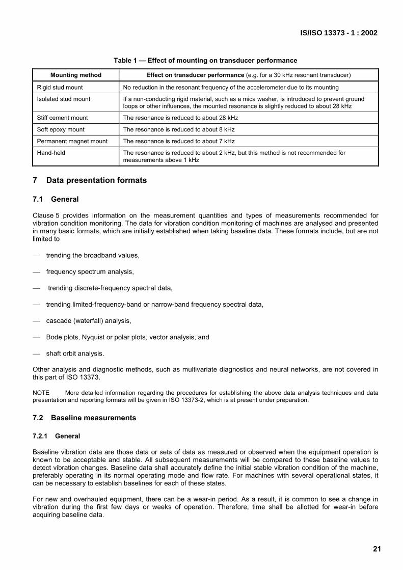
Table 1 — Effect of mounting on transducer performance

Mounting method Effect on transducer performance (e.g. for a 30 kHz resonant transducer)

Rigid stud mount No reduction in the resonant frequency of the accelerometer due to its mounting

Isolated stud mount If a non-conducting rigid material, such as a mica washer, is introduced to prevent ground loops or other influences, the mounted resonance is slightly reduced to about 28 kHz

Stiff cement mount The resonance is reduced to about 28 kHz

Soft epoxy mount The resonance is reduced to about 8 kHz

Permanent magnet mount The resonance is reduced to about 7 kHz

Hand-held The resonance is reduced to about 2 kHz, but this method is not recommended for measurements above 1 kHz

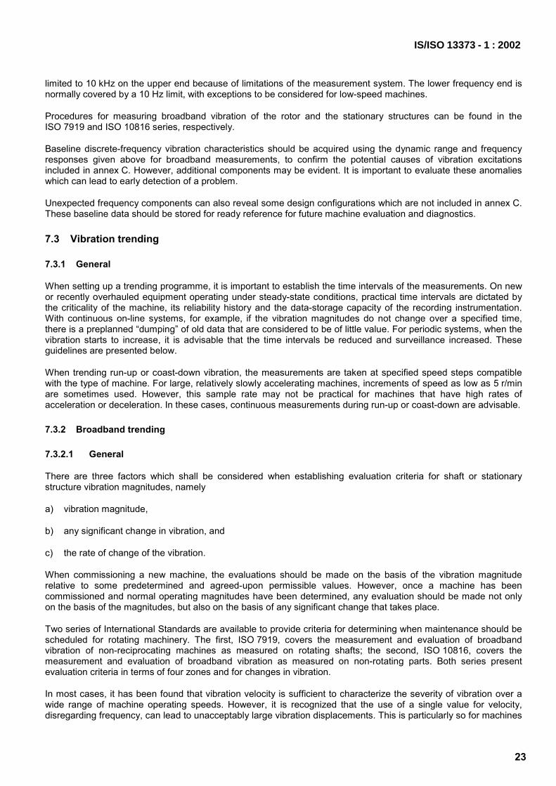
7 Data presentation formats

7.1 General

Clause 5 provides information on the measurement quantities and types of measurements recommended for vibration condition monitoring. The data for vibration condition monitoring of machines are analysed and presented in many basic formats, which are initially established when taking baseline data. These formats include, but are not limited to

trending the broadband values,

frequency spectrum analysis,

trending discrete-frequency spectral data,

trending limited-frequency-band or narrow-band frequency spectral data,

cascade (waterfall) analysis,

Bode plots, Nyquist or polar plots, vector analysis, and

shaft orbit analysis.

Other analysis and diagnostic methods, such as multivariate diagnostics and neural networks, are not covered in this part of ISO 13373.

NOTE More detailed information regarding the procedures for establishing the above data analysis techniques and data presentation and reporting formats will be given in ISO 13373-2, which is at present under preparation.

7.2 Baseline measurements

7.2.1 General

Baseline vibration data are those data or sets of data as measured or observed when the equipment operation is known to be acceptable and stable. All subsequent measurements will be compared to these baseline values to detect vibration changes. Baseline data shall accurately define the initial stable vibration condition of the machine, preferably operating in its normal operating mode and flow rate. For machines with several operational states, it can be necessary to establish baselines for each of these states.

For new and overhauled equipment, there can be a wear-in period. As a result, it is common to see a change in vibration during the first few days or weeks of operation. Therefore, time shall be allotted for wear-in before acquiring baseline data.

IS/ISO 13373 - 1 : 2002

21

22

For equipment which has been operating for a significant period and monitored for the first time, a baseline can still be established as a trending reference point.

Vibration and operating data should be acquired at a sufficient number of intervals to establish that the machine has reached stable conditions. At this time, full baseline data should be taken and compared to applicable standards, as available, to determine the operability of the machine. The baseline signature should also be examined for evidence of undesirable conditions, such as shaft instabilities.

These data are the basis upon which future machine problems will be detected and diagnosed. These data shall be stored so that they are easily retrievable and secure.

Baseline vibration data can consist of all the potential vibration parameters that are commonly used to define the vibration condition of the machine. The more comprehensive the initial definition of baseline, the greater the likelihood of properly detecting, analysing and tracking the deterioration of the machine. The data used to define a vibration baseline for a condition monitoring programme may include all or some of the following:

broadband magnitude (displacement, velocity and/or acceleration);

time signal and waveform;

rotational frequency;

amplitude at once-per-revolution;

vibration vectors (amplitude and phase);

frequency spectrum analysis of the vibration signals at steady state;

run-up/coast-down frequency response data (e.g. Bode plots, waterfall plots, polar plots);

shaft orbit analysis;

shaft centreline position.

The completeness of the baseline signature definition depends on the following:

the importance of the machine;

the previous history of the machine;

the analysis equipment available;

the capabilities of the personnel,

other factors.

The locations at which data are obtained need not and should not be limited to those locations that are to be continuously monitored. It is recommended that the baseline be a comprehensive vibration analysis, normally encompassing more measurement points, directions, broader frequency range and finer resolution than are required in a routine programme. After either continuous or periodic monitoring of a relatively few points have established that a change has taken place, a repeat of the procedures used for baseline analysis can be prepared to help define the cause of the vibration change.

7.2.2 Broadband vibration

Unless prior knowledge dictates otherwise, the baseline broadband vibration should be acquired covering a sufficient dynamic range and frequency response to include all forcing excitations of interest within the machine. In general, this requires r.m.s. velocity 0,1 mm/s to 100 mm/s with frequency ranges of 0,2 times the lowest rotational frequency to 3,5 times the highest frequency of interest. For most machines, this frequency range will normally be

IS/ISO 13373 - 1 : 2002

limited to 10 kHz on the upper end because of limitations of the measurement system. The lower frequency end is normally covered by a 10 Hz limit, with exceptions to be considered for low-speed machines.

Procedures for measuring broadband vibration of the rotor and the stationary structures can be found in the ISO 7919 and ISO 10816 series, respectively.

Baseline discrete-frequency vibration characteristics should be acquired using the dynamic range and frequency responses given above for broadband measurements, to confirm the potential causes of vibration excitations included in annex C. However, additional components may be evident. It is important to evaluate these anomalies which can lead to early detection of a problem.

Unexpected frequency components can also reveal some design configurations which are not included in annex C. These baseline data should be stored for ready reference for future machine evaluation and diagnostics.

7.3 Vibration trending

7.3.1 General

When setting up a trending programme, it is important to establish the time intervals of the measurements. On new or recently overhauled equipment operating under steady-state conditions, practical time intervals are dictated by the criticality of the machine, its reliability history and the data-storage capacity of the recording instrumentation. With continuous on-line systems, for example, if the vibration magnitudes do not change over a specified time, there is a preplanned “dumping” of old data that are considered to be of little value. For periodic systems, when the vibration starts to increase, it is advisable that the time intervals be reduced and surveillance increased. These guidelines are presented below.

When trending run-up or coast-down vibration, the measurements are taken at specified speed steps compatible with the type of machine. For large, relatively slowly accelerating machines, increments of speed as low as 5 r/min are sometimes used. However, this sample rate may not be practical for machines that have high rates of acceleration or deceleration. In these cases, continuous measurements during run-up or coast-down are advisable.

7.3.2 Broadband trending

7.3.2.1 General

There are three factors which shall be considered when establishing evaluation criteria for shaft or stationary structure vibration magnitudes, namely

a) vibration magnitude,

b) any significant change in vibration, and

c) the rate of change of the vibration.

When commissioning a new machine, the evaluations should be made on the basis of the vibration magnitude relative to some predetermined and agreed-upon permissible values. However, once a machine has been commissioned and normal operating magnitudes have been determined, any evaluation should be made not only on the basis of the magnitudes, but also on the basis of any significant change that takes place.

Two series of International Standards are available to provide criteria for determining when maintenance should be scheduled for rotating machinery. The first, ISO 7919, covers the measurement and evaluation of broadband vibration of non-reciprocating machines as measured on rotating shafts; the second, ISO 10816, covers the measurement and evaluation of broadband vibration as measured on non-rotating parts. Both series present evaluation criteria in terms of four zones and for changes in vibration.

In most cases, it has been found that vibration velocity is sufficient to characterize the severity of vibration over a wide range of machine operating speeds. However, it is recognized that the use of a single value for velocity, disregarding frequency, can lead to unacceptably large vibration displacements. This is particularly so for machines

IS/ISO 13373 - 1 : 2002

23

24

with low operating speeds when the once-per-revolution vibration component is dominant. Similarly, constant velocity criteria for machines with high operating speeds, or with vibration at high frequencies generated by machine component parts can lead to unacceptable accelerations. Consequently, acceptance criteria based on velocity will take the general form of Figure 11. This indicates the upper and lower frequency limits fu and fl and shows that below a defined frequency fx and above a defined frequency fy the allowable vibration velocity is a function of the vibration frequency. However, for vibration frequencies between fx and fy, a constant velocity criterion applies. The evaluation criteria and the values of fl, fu, fx and fy for specific machine types are given in the relevant parts of ISO 10816.

1 Constant displacement 2 Constant velocity 3 Constant acceleration

Figure 11 — Vibration zones

The vibration of newly commissioned machines would normally fall within zone A. Machines with vibration magnitudes within zone B are normally considered acceptable for unrestricted long-term operation.

Machines with vibration magnitudes within zone C are normally considered unsatisfactory for long-term continuous operation. Generally, the machine may be operated for a limited period in zone C until a suitable opportunity arises for remedial action. Vibration magnitudes within zone D are normally considered to be of sufficient severity to cause damage to the machine.

The ALARM values can vary considerably, up or down, for specific machines. The values chosen will normally be set relative to baseline magnitudes determined from experience for the measurement positions and directions for that particular machine or class of machines.

It is recommended that the ALARM value should be set higher than the baseline by an amount equal to 25 % of the upper limit of zone B. If the baseline is low, the ALARM may be below zone C.

IS/ISO 13373 - 1 : 2002

In most cases where there is no established baseline, for example a new machine, the initial ALARM value should be based either on experience with other similar machines or relative to agreed acceptance values. After a period of time, the steady-state baseline values should be established and the ALARM settings adjusted accordingly.

In either case it is recommended that the ALARM value should not normally exceed 1,25 times the upper limit of zone B.

If the steady-state baseline changes (for example after a machine overhaul), the ALARM setting may need to be revised accordingly.

The TRIP values will generally relate to the mechanical integrity of the machine and will be dependent on specific design features which have been introduced to enable the machine to withstand abnormal dynamic forces. The values used will therefore generally be the same for all machines of similar design and would not normally be related to the steady-state baseline value used for setting ALARMS.

There may, however, be differences for machines of different design, and it is not possible to give clear guidelines for absolute TRIP magnitudes. In general, the TRIP magnitude will be within zone C or D, but is recommended that the TRIP value should not exceed 1,25 times the upper limit of zone C.

The zone boundaries recommended in the ISO 7919 and ISO 10816 series are based on statistical analysis of a worldwide industry survey.

The action required or recommended when equipment is operating in each of these zones depends on the rate at which the vibration magnitude is changing.

These same criteria should be used to specify the maximum period for obtaining data, or review of the data, obtained by continuous monitoring of equipment. The interval for monitoring or data review will vary depending on the magnitude of vibration observed and/or the rate at which the vibration magnitude is changing. These actions are described below and depicted in Figures 12 and 13.

7.3.2.2 Case 1: Equipment vibration magnitude is in the “normal range”

In this case the following action guidelines apply to the vibration trend curve in zone B of Figure 12.

a) If there is no significant change in the magnitude from the previous data, then no action is required.

b) If the vibration is increasing, the rate of increase is linear, and the magnitude is projected not to exceed the upper limit of the normal range before the next scheduled monitoring, no action is required. However, if the projected magnitude indicates that it will exceed that upper limit before the next monitoring, schedule more frequent monitoring as the upper limit is reached.

c) If the rate of increase is non-linear, or the rate of change increases 25 % from a previous reading within a preset time frame, confirm the rate by continuous monitoring, or schedule more frequent monitoring and consider implementing a diagnostics programme.

7.3.2.3 Case 2: Current vibration magnitude is in the ALARM zone

In this case the following action guidelines apply to the vibration trend curve in zone C of Figure 13.

a) If there is no change in the magnitude, maintain the same monitoring intervals.

b) If the magnitude is increasing at a linear rate and is projected to exceed the action magnitude prior to scheduled maintenance, or before the next scheduled surveillance, or the rate of increase is non-linear, confirm the rate of increase by continuous or more frequent monitoring and reschedule maintenance. Increase the monitoring frequency to ensure that three data points are collected prior to rescheduled maintenance. A diagnostics programme is recommended to define the problem and maintenance required. Should a decrease in vibration magnitude be observed, biweekly monitoring rate should continue and diagnostics are recommended.

IS/ISO 13373 - 1 : 2002

25

26

1 Action required a Peak-to-peak displacement (mm) or r.m.s. velocity (mm/s). 2 Alert b For defined vibration limits, see ISO 7919 or ISO 10816. 3 Normal c Projected occurrence of action required. d Follow-up required within 48 h.

Figure 12 — Broadband vibration as measured on rotating shaft or machine structure — Vibration magnitude in the “normal range”

IS/ISO 13373 - 1 : 2002

1 Action required a Peak-to-peak displacement (mm) or r.m.s. velocity (mm/s). 2 Alert b For defined vibration limits, see ISO 7919 or ISO 10816. 3 Normal c Projected occurrence of action required. d Follow-up required within 48 h.

Figure 13 — Broadband vibration as measured on rotating shaft or machine structure — Vibration magnitude in the ALARM zone

7.3.3 Vibration during run-up/coast-down

Run-up/coast-down vibration as defined here is the vibration information obtained during the start-up and shut-down operations of a machine train. This type of data can provide insight into the mechanical condition of the machinery that cannot be obtained during steady-state operation. Unbalance response, the presence of structural and component resonance, including critical speeds, damping, electromagnetic anomalies, rubs and shaft cracks are all examples of conditions that are best detected and analysed from run-up/coast-down data. The spectra of

IS/ISO 13373 - 1 : 2002

27

28

run-up/coast-down data contain a third dimension, either time or rotating speed. Thus, run-up/coast-down displays are more complex than equivalent steady-state spectra and, if plotted versus speed, require a once-per-revolution reference. The vibration data are usually displayed in presentation formats such as Bode plots, Nyquist/polar plots, Campbell diagrams and cascade (waterfall) diagrams.

Run-up/coast-down vibration is an important part of the baseline vibration data. The more comprehensive the initial testing, the greater the likelihood of properly detecting, diagnosing and tracking the deterioration of the machine.

7.3.4 Transient-vibration trending

Although transient displays are more complex than equivalent steady-state displays, they also have to be trended with time to detect the presence of changes in the machine. Comprehensive analysis of the complex three-dimensional data will detect anomalies which may not be disclosed in steady-state operation.

Even if the speed of a machine remains constant, transient operations can occur with variations in environmental conditions (temperature, pressure, etc.), load, process parameters, etc. Therefore, it is essential that the measurement of transient vibration associated with these changes be trended under the same operating conditions as far as possible.

7.4 Discrete-frequency vibration

7.4.1 General

Broadband vibration does not always provide sufficient information to identify the specific cause of an ALARM. This is especially true for complex equipment where several excitation frequencies appear in the frequency spectrum. In such cases it is advisable to split the broadband vibration signal into discrete frequency components (amplitude and/or phase). In most cases individual frequencies can be matched with corresponding moving machine parts. When these vibration components change, irregularities or machine damage can often be detected even at their earliest stage. Mechanically or thermally induced rotor unbalance, self-excited vibration, rubs, alignment changes, bearing or gear damage and rotor cracks are just a few of the types of problems that can be detected by discrete-frequency analysis.

In normal practices, a reference spectrum of the machine is recorded during commissioning or after overhaul, which becomes the baseline signature. This reference spectrum permits comparison with later frequency analyses in order to detect any change. Care should be taken to ensure that the same bandwidth and window function are used when comparing results from FFT analysis.

A sample frequency spectrum plot is given in Figure 14. It clearly shows vibration amplitudes at specific frequencies. It is important to evaluate the source of significant frequency peaks as their magnitudes can be abnormal, and when immediately investigated can lead to early detection of a problem. Unexpected frequency components can also reveal some design configuration which is not included in annex C.

NOTE More detailed procedures for converting a broadband time trace to a frequency spectrum will be given in ISO 13373-2, which is at present under preparation.

7.4.2 Trending of discrete-frequency vibration

Trending of the discrete frequencies within a machinery vibration spectrum provides more comprehensive data for establishing vibration limits. Figure 15 shows a typical example of the trending of the fundamental frequency and its harmonics as a function of time.

IS/ISO 13373 - 1 : 2002

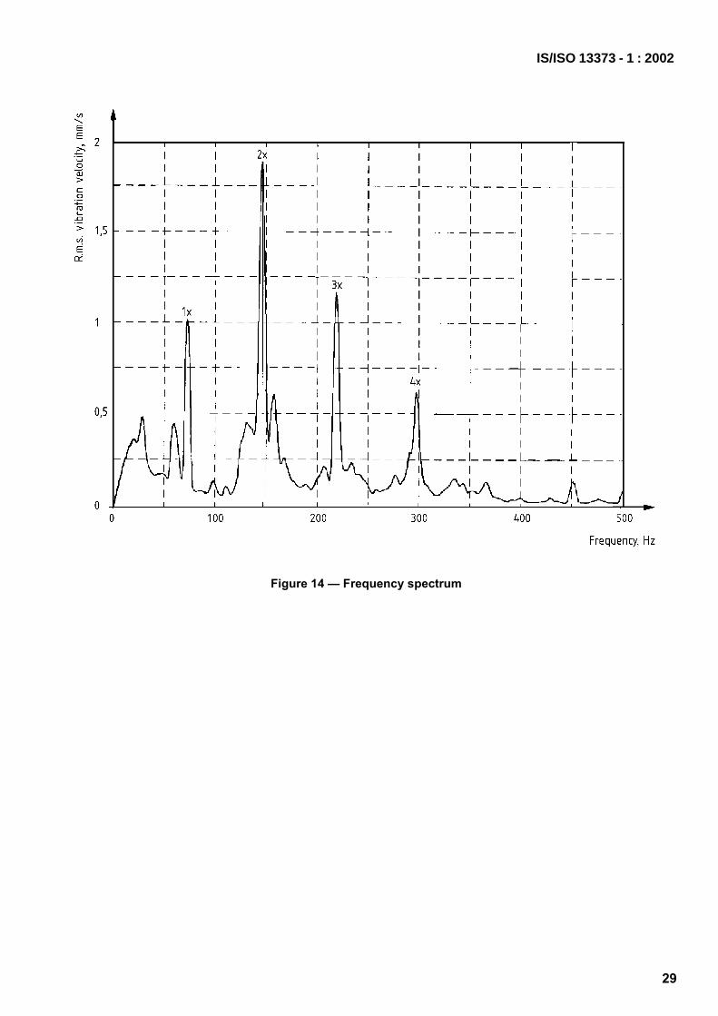
Figure 14 — Frequency spectrum

IS/ISO 13373 - 1 : 2002

29

30

NOTE “sub” means subsynchronous components.

Figure 15 — Discrete-frequency vibration trends

7.5 Analysis of high-frequency vibration envelope

In some cases, changes in the machine vibratory state are more readily characterized by analysis of the high-frequency vibration envelope. There are a number of different techniques available but these are outside the scope of this part of ISO 13373.

8 Data analysis and communication

This part of ISO 13373 gives general guidelines to be followed for the acquisition of data for vibration condition monitoring of machines, in order to obtain meaningful data while also considering practical and economic constraints.

NOTE Further analysis and presentation formats of the vibration data will be given in ISO 13373-2, which is at present under preparation.

IS/ISO 13373 - 1 : 2002

Annex A (informative)

Guidelines for types and locations of measurements

Table A.1 consists of a listing of the various types of machines where vibration detectors are typically used to monitor the condition of a machine. Also included are the types of vibration transducers that are normally applied, together with guidance on their directions and locations. In many applications a reduced number of measurement locations may be used.

Identifications of the machines, transducers and locations are by no means limited to the information given in Table A.1; these are basic guidelines. However, for machine types not listed in Table A.1, it may be necessary to vary the transducer types and locations, as appropriate, for adequate vibration condition monitoring.

IS/ISO 13373 - 1 : 2002

31

32

Tabl

e A.

1 —

Typ

es a

nd lo

catio

ns o

f mea

sure

men

t

Mac

hine

type

Ev

alua

tion

para

met

ers

Tran

sduc

er ty

pe

Mea

sure

men

t loc

atio

ns

Dire

ctio

n St

anda

rd

refe

renc

e Se

e no

te

Larg

e st

eam

turb

ine

gene

rato

r set

s w

ith

fluid

-film

bea

rings

Pow

er g

ener

atio

n

rela

tive

disp

lace

men

t or

ab

solu

te d

ispl

acem

ent

velo

city

or a

ccel

erat

ion

shaf

t axi

al d

ispl

acem

ent

phas

e re

fere

nce

and

spee

d

non-

cont

actin

g tra

nsdu

cer

non-

cont

actin

g an

d se

ism

ic

trans

duce

r com

bina

tion

velo

city

tran

sduc

er o

r acc

eler

omet

er

non-

cont

actin

g tra

nsdu

cer o

r axi

al

prob

e ed

dy c

urre

nt/in

duct

ive/

optic

al

trans

duce

r

shaf

t at e

ach

bear

ing

each

bea

ring

hous

ing

each

bea

ring

hous

ing

thru

st c

olla

r sh

aft

radi

al ±

45°

or

X a

nd Y

ra

dial

X

and

Y ax

ial Z

ra

dial

ISO

791

9-2

ISO

108

16-2

1

Med

ium

and

sm

all

indu

stria

l ste

am

turb

ines

with

flui

d-fil

m

bear

ings

Mec

hani

cal d

rives

, po

wer

gen

erat

ion

rela

tive

disp

lace

men

t ve

loci

ty o

r acc

eler

atio

n sh

aft a

xial

dis

plac

emen

t ph

ase

refe

renc

e an

d sp

eed

non-

cont

actin

g tra

nsdu

cer

velo

city

tran

sduc

er o

r acc

eler

omet

er

non-

cont

actin

g tra

nsdu

cer o

r axi

al

prob

e ed

dy c

urre

nt/in

duct

ive/

optic

al

trans

duce

r

shaf

t at e

ach

bear

ing

each

bea

ring

hous

ing

and

turb

ine

hous

ing

thru

st c

olla

r sh

aft

radi

al ±

45°

or

X a

nd Y

ra

dial

X

and

Y ax

ial Z

ra

dial

ISO

791

9-3

ISO

108

16-3

Smal

l ind

ustr

ial s

team

tu

rbin

es w

ith ro

lling

el

emen

t bea

rings

velo

city

or a

ccel

erat

ion

phas

e re

fere

nce

and

spee

d

velo

city

tran

sduc

er o

r acc

eler

omet

er

eddy

cur

rent

/indu

ctiv

e/op

tical

tra

nsdu

cer

each

bea

ring

hous

ing

and

turb

ine

hous

ing

shaf

t

radi

al X

and

Y,

axi

al Z

ra

dial

ISO

108

16-3

Larg

e an

d m

ediu

m

indu

stria

l gas

turb

ines

w

ith fl

uid-

film

bea

rings

rela

tive

or a

bsol

ute

disp

lace

men

t ve

loci

ty o

r acc

eler

atio

n sh

aft a

xial

dis

plac

emen

t ph

ase

refe

renc

e an

d sp

eed

non-

cont

actin

g tra

nsdu

cer

velo

city

tran

sduc

er o

r acc

eler

omet

er

non-

cont

actin

g tra

nsdu

cer o

r axi

al

prob

e ed

dy c

urre

nt/in

duct

ive/

optic

al

trans

duce

r

shaf

t at e

ach

bear

ing

each

bea

ring

thru

st c

olla

r sh

aft

radi

al ±

45°

ra

dial

X

and

Y ax

ial Z

ra

dial

ISO

791

9-4

ISO

108

16-4

IS/ISO 13373 - 1 : 2002

Tabl

e A.

1 (c

ontin

ued)

Mac

hine

type

Ev

alua

tion

para

met

ers

Tran

sduc

er ty

pe

Mea

sure

men

t loc

atio

ns

Dire

ctio

n St

anda

rd

refe

renc

e Se

e no

te

Hyd

roel

ectr

ic tu

rbin

es

with

flui

d-fil

m b

earin

gs

rela

tive

disp

lace

men

t ve

loci

ty o

r acc

eler

atio

n sh

aft a

xial

dis

plac

emen

t ph

ase

refe

renc

e an

d sp

eed

non-

cont

actin

g tra

nsdu

cer

velo

city

tran

sduc

er o

r acc

eler

omet

er

non-

cont

actin

g tra

nsdu

cer o

r axi

al

prob

e ed

dy c

urre

nt/in

duct

ive/

optic

al

trans

duce

r

shaf

t at s

elec

ted

bear

ings

ea

ch b

earin

g ho

usin

g an

d tu

rbin

e ca

sing

th

rust

col

lar

shaf

t

radi

al 9

0°

apar

t ra

dial

90°

ap

art

axia

l Z

radi

al

ISO

791

9- 5

IS

O 1

0816

-5

2 3

Larg

e pu

mps

with

flui

d-fil

m b

earin

gs

rela

tive

or a

bsol

ute

disp

lace

men

t no

n-co

ntac

ting

trans

duce

r sh

aft a

t eac

h be

arin

g ra

dial

± 4

5°

ISO

791

9-3,

IS

O 7

919-

5

4

∑ B

oile

r fee

d ∑

Circ

ulat

ing

∑ P

roce

ss

velo

city

or a

ccel

erat

ion

shaf

t axi

al d

ispl

acem

ent

phas

e re

fere

nce

and

spee

d

velo

city

tran

sduc

er o

r acc

eler

omet

er

non-

cont

actin

g tra

nsdu

cer o

r axi

al

prob

e ed

dy c

urre

nt/in

duct

ive/

optic

al

trans

duce

r

bear

ing

hous

ings

th

rust

col

lar

shaf

t

radi

al X

an

d Y

axia

l Z

radi

al

ISO

108

16-3

, IS

O 1

0816

-5

Med

ium

and

sm

all

pum

ps w

ith fl

uid-

film

be

arin

gs

rela

tive

disp

lace

men

t (u

ncom

mon

) ve

loci

ty o

r acc

eler

atio

n sh

aft a

xial

dis

plac

emen

t ph

ase

refe

renc

e an

d sp

eed

non-

cont

actin

g tra

nsdu

cer

velo

city

tran

sduc

er o

r acc

eler

omet

er

velo

city

non

-con

tact

ing

trans

duce

r or

axi

al p

robe

ed

dy c

urre

nt/in

duct

ive/

optic

al

trans

duce

r

shaf

t at e

ach

bear

ing

bear

ing

hous

ings

th

rust

col

lar

shaf

t

radi

al ±

45°

ra

dial

X

and

Y ax

ial Z

ra

dial

ISO

791

9- 3

IS

O 1

0816

- 3

4 5

Med

ium

and

sm

all

pum

ps w

ith ro

lling

el

emen

t bea

rings

velo

city

or a

ccel

erat

ion

phas

e re

fere

nce

and

spee

d

velo

city

tran

sduc

er o

r acc

eler

omet

er

eddy

cur

rent

/indu

ctiv

e/op

tical

tra

nsdu

cer

each

bea

ring

and

pum

p ho

usin

g sh

aft

radi

al X

an

d Y,

axi

al

Z radi

al

ISO

108

16-3

4 5

Vert

ical

ly m

ount

ed

pum

ps

Rea

ctor

coo

lant

C

oola

nt p

umps

rela

tive

disp

lace

men

t ve

loci

ty o

r acc

eler

atio

n sh

aft a

xial

dis

plac

emen

t ph

ase

refe

renc

e an

d sp

eed

non-

cont

actin

g tra

nsdu

cer

velo

city

tran

sduc

er o

r acc

eler

omet

er

non-

cont

actin

g tra

nsdu

cer o

r axi

al

shaf

t pro

be

eddy

cur

rent

/indu

ctiv

e/op

tical

tra

nsdu

cer

mot

or/p

ump

shaf

ts a

t eac

h ac

cess

ible

bea

ring,

top

pum

p be

arin

g (m

inim

um)

mot

or a

nd e

ach

acce

ssib

le

bear

ing

hous

ing

mot

or s

haft

shaf

t

radi

al 9

0°

apar

t ra

dial

90°

ap

art

axia

l Z

radi

al

ISO

791

9- 5

IS

O 1

0816

-3,

ISO

108

16-5

3

IS/ISO 13373 - 1 : 2002

33

34

Tabl

e A.

1 (c

ontin

ued)

Mac

hine

type

Ev

alua

tion

para

met

ers

Tran

sduc

er ty

pe

Mea

sure

men

t loc

atio

ns

Dire

ctio

n St

anda

rd

refe

renc

e Se

e no

te

Larg

e el

ectr

ic m

otor

s an

d ge

nera

tors

with

flu

id-fi

lm b

earin

gs

rela

tive

disp

lace

men

t ve

loci

ty o

r acc

eler

atio

n sh

aft a

xial

dis

plac

emen

t ph

ase

refe

renc

e an

d sp

eed

non-

cont

actin

g tra

nsdu

cer

velo

city

tran

sduc

er o

r acc

eler

omet

er

non-

cont

actin

g tra

nsdu

cer o

r axi

al

prob

e ed

dy c

urre

nt/in

duct

ive/

optic

al

trans

duce

r

shaf

t at e

ach

bear

ing

hous

ing

thru

st c

olla

r sh

aft

radi

al ±

45°

ra

dial

X

and

Y ax

ial Z

ra

dial

ISO

791

9-3

ISO

108

16-3

, IS

O 1

0816

-5

Med

ium

and

sm

all

mot

ors

with

rolli

ng

elem

ent b

earin

gs

velo

city

or a

ccel

erat

ion

phas

e re

fere

nce

and

spee

d

velo

city

tran

sduc

er o

r acc

eler

omet

er

eddy

cur

rent

/indu

ctiv

e/op

tical

tra

nsdu

cer

each

bea

ring

and

mot

or

hous

ing

shaf

t

radi

al X

an

d Y,

axi

al

Z radi

al

ISO

108

16-3

5

Com

pres

sors

–

pack

age

cent

rifug

al

(four

-pos

ter)

, with

flui

d-fil

m b

earin

gs a

nd ri

gid

hous

ings

rela

tive

disp

lace

men

t ve

loci

ty o

r acc

eler

atio

n ph

ase

refe

renc

e an

d sp

eed

non-

cont

actin

g tra

nsdu

cer

velo

city

tran

sduc

er o

r acc

eler

omet

er

eddy

cur

rent

/indu

ctiv

e/op

tical

tra

nsdu

cer

each

bea

ring,

pin

ion

hous

ing

and

ball

gear

sha

ft at

eac

h be

arin

g or

gea

r mes

h ea

ch s

haft

radi

al ±

45°

ra

dial

X

and

Y ra

dial

ISO

791

9-3

ISO

108

16-3

Com

pres

sors

–

cent

rifug

al p

roce

ss

rela

tive

disp

lace

men

t ve

loci

ty o

r acc

eler

atio

n sh

aft a

xial

dis

plac

emen

t ph

ase

refe

renc

e an

d sp

eed

(if d

rivin

g th

roug

h ge

ar

box)

non-

cont

actin

g tra

nsdu

cer

velo

city

tran

sduc

er o

r acc

eler

omet

er

non-

cont

actin

g tra

nsdu

cer o

r axi

al

prob

e ed

dy c

urre

nt/in

duct

ive/

optic

al

trans

duce

r

shaf

t at e

ach

bear

ing

bear

ing

hous

ings

th

rust

col

lar o

r sha

ft en

d sh

aft

radi

al ±

45°

ra

dial

X

and

Y ax

ial Z

ra

dial

ISO

791

9-3

ISO

108

16-3

6

Com

pres

sors

– s

crew

-ty

pe w

ith tw

o in

terlo

ckin

g sh

afts

, flu

id-fi

lm b

earin

gs

rela

tive

disp

lace

men

t ve

loci

ty o

r acc

eler

atio

n sh

aft a

xial

dis

plac

emen

t ph

ase

angl

e of

eac

h sh

aft

non-

cont

actin

g tra

nsdu

cer

velo

city

tran

sduc

er o

r acc

eler

omet

er

non-

cont

actin

g tra

nsdu

cer o

r axi

al

prob

e ph

ase

refe

renc

e tra

nsdu

cer

shaf

t at e

ach

bear

ing

bear

ing

caps

and

co

mpr

esso

r hou

sing

th

rust

col

lar

each

sha

ft

radi

al ±

45°

ra

dial

X a

nd

Y, a

xial

Z

axia

l Z

radi

al

ISO

108

16-1

IS/ISO 13373 - 1 : 2002

Tabl

e A.

1 (c

ontin

ued)

Mac

hine

type

Ev

alua

tion

para

met

ers

Tran

sduc

er ty

pe

Mea

sure

men

t loc

atio

ns

Dire

ctio

n St

anda

rd

refe

renc

e Se

e no

te

Com

pres

sors

– s

crew

-ty

pe w

ith tw

o in

terlo

ckin

g sh

afts

, ro

lling

ele

men

t be

arin

gs

velo

city

or a

ccel

erat

ion

phas

e an

gle

of e

ach

shaf

t

velo

city

tran

sduc

er o

r acc

eler

omet

er

eddy

cur

rent

/indu

ctiv

e/op

tical

tra

nsdu

cer

bear

ing

caps

and

co

mpr

esso

r hou

sing

ea

ch s

haft

radi

al X

and

Y,

axi

al Z

ra

dial

ISO

108

16-1

Gea

rs –

larg

e w

ith fl

uid-

film

bea

rings

re

lativ

e di

spla

cem

ent

velo

city

and

/or

acce

lera

tion

shaf

t axi

al d

ispl

acem

ent

non-

cont

actin

g tra

nsdu

cer

velo

city

tran

sduc

er a

nd/o

r ac

cele

rom

eter

no

n-co

ntac

ting

trans

duce

r

shaf

t at e

ach

bear

ing

bear

ing

caps

and

gea

r cas

e sh

aft e

nds

radi

al ±

45°

ra

dial

X

and

Y, a

xial

Z ax

ial Z

Gea

rs –

with

rolli

ng

elem

ent b

earin

gs

velo

city

and

/or

acce

lera

tion

velo

city

tran

sduc

er a

nd/o

r ac

cele

rom

eter

be

arin

g ca

ps a

nd g

ear

hous

ing

radi

al X

and

Y,

axi

al Z

Fans

– la

rge

with

flui

d-fil

m b

earin

gs

rela

tive

disp

lace

men

t ve

loci

ty o

r acc

eler

atio

n sh

aft a

xial

dis

plac

emen

t ph

ase

refe

renc

e an

d sp

eed

non-

cont

actin

g tra

nsdu

cer

(unc

omm

on)

velo

city

tran

sduc

er o

r acc

eler

omet

er

non-

cont

actin

g tra

nsdu

cer o

r axi

al

prob

e ed

dy c

urre

nt/in

duct

ive/

optic

al

trans

duce

r

bear

ing

hous

ings

cas

ing

bear

ing

hous

ings

th

rust

col

lar o

r sha

ft en

d sh

aft

radi

al ±

45°

ra

dial

X

and

Y ax

ial Z

ra

dial

ISO

791

9-3

ISO

108

16-3

7 8

Fans

– m

ediu

m a

nd

smal

l with

rolli

ng

elem

ent b

earin

gs

velo

city

/acc

eler

atio

n ve

loci

ty tr

ansd

ucer

or a

ccel

erom

eter

ea

ch b

earin

g ca

p an

d fa

n ho

usin

g ra

dial

X a

nd

Y, a

xial

Z

ISO

108

16-3

Cen

trifu

ges

rela

tive

disp

lace

men

t ve

loci

ty o

r acc

eler

atio

n sh

aft a

xial

dis

plac

emen

t ph

ase

refe

renc

e an

d sp

eed

non-

cont

actin

g tra

nsdu

cer

velo

city

tran

sduc

er o

r acc

eler

omet

er

non-

cont

actin

g tra

nsdu

cer o

r axi

al

prob

e ed

dy c

urre

nt/in

duct

ive/

optic

al

trans

duce

r

shaf

t at e

ach

bear

ing

(if

acc

essi

ble)

ea

ch a

cces

sibl

e be

arin

g th

rust

col

lar

shaf

t

radi

al ±

45°

ra

dial

X

and

Y ax

ial Z

ra

dial

ISO

108

16-1

IS/ISO 13373 - 1 : 2002

35

36

Tabl

e A.

1 (c

oncl

uded

)

Mac

hine

type

Ev

alua

tion

para

met

ers

Tran

sduc

er ty

pe

Mea

sure

men

t loc

atio

ns

Dire

ctio

n St

anda

rd

refe

renc

e Se

e no

te

Pulp

refin

ers

rela

tive

disp

lace

men

t ve

loci

ty o

r acc

eler

atio

n ph

ase

refe

renc

e an

d sp

eed

non-

cont

actin

g tra

nsdu

cer

velo

city

tran

sduc

er o

r acc

eler

omet

er

eddy

cur

rent

/indu

ctiv

e/op

tical

tra

nsdu

cer

shaf

t at e

ach

bear

ing

bear

ing

caps

on

eac

h sh

aft

radi

al X

an

d Y

radi

al X

an

d Y

radi

al

ISO

108

16-1

NO

TE 1

O

rthog

onal

mea

sure

men

ts a

t ± 4

5° a

re n

orm

ally

use

d fo

r con

ditio

n m

onito

ring.

Ver

tical

and

hor

izon

tal (

X an

d Y)

loca

tions

are

acc

epta

ble

alte

rnat

ives

; tha

t may

pro

vide

mor

e m

eani

ngfu

l dat

a pa

rticu

larly

if th

ese

are

the

prin

cipa

l stif

fnes

s di

rect

ions

.

NO

TE 2

M

easu

ring

both

the

d.c.

dis

plac

emen

t and

the

dyna

mic

dis

plac

emen

ts is

alw

ays

reco

mm

ende

d pr

actic

e. It

is m

ore

impo

rtant

on

hydr

oele

ctric

turb

ines

due

to th

e re

lativ

ely

larg

er

radi

al b

earin

g cl

eara

nces

.

NO

TE 3

Fo

r ver

tical

mac

hine

s, m

easu

rem

ents

sho

uld

be m

ade

in th

e ax

es o

f maj

or a

nd m

inor

stif

fnes

s di

rect

ions

, usu

ally

rela

ted

to th

e in

let l

ocat

ion.

NO

TE 4

Pu

mp

vibr

atio

n va

ries

sign

ifica

ntly

with

ope

ratin

g co

nditi

on. I

deal

ly, o

pera

tion

at th

e Be

st E

ffici

ency

Poi

nt (B

EP) w

ill ha

ve th

e le

ast v

ibra

tions

. Ope

ratin

g co

ntin

uous

ly a

t a p

oint

ot

her t

han

the

BEP

will

prod

uce

incr

ease

d vi

brat

ions

. In

any

case

, rea

ding

s sh

ould

alw

ays

be ta

ken

unde

r the

sam

e op

erat

ing

cond

ition

s fo

r com

paris

on.

NO

TE 5

Po

rtabl

e sy

stem

s ar

e co

mm

only

use

d as

med

ium

and

sm

all s

ize

equi

pmen

t do

not u

sual

ly ju

stify

on-

line

syst

ems.

NO

TE 6

If

not d

irect

ly c

oupl

ed, t

wo

keyw

ay re

fere

nces

are

requ

ired.

NO

TE 7

O

n la

rge

axia

l-flo

w fa

ns, i

f the

bea

rings

and

driv

e sh

afts

are

not

acc

essi

ble,

mea

sure

men

ts in

the

X an

d Y

dire

ctio

ns o

n th

e fa

n ho

usin

g sh

ould

be

take

n.

NO

TE 8

O

verh

ung

cons

truct

ion:

mai

n lo

ad-c

arry

ing

bear

ing

only

.

IS/ISO 13373 - 1 : 2002

Annex B (informative)

Typical information to be recorded

B.1 Machine details

For each machine being monitored, the following information should be recorded:

unique machine identifier (e.g. equipment code);

machine type (e.g. motor, generator, turbine, compressor, pump, fan);

power source (e.g. electric, steam, gas, reciprocating internal combustion (RIC), diesel, hydraulic);

rated speed (e.g. r/min or Hz);

rated power (e.g. kW);

configuration (e.g. direct, belt or shaft driven);

machine support (e.g. rigid or resiliently mounted);

shaft coupling (e.g. rigid or flexible).

The following additional information may also be recorded:

function (e.g. driver or driven).

B.2 Measurements

For each measuring system, the following information should be recorded:

date and time (including time zone) of measurement;

instrument type;

transducer type1) (e.g. eddy current, velocity, accelerometer);

transducer method of attachment (e.g. probe, magnet, stud, adhesive);

measurement location1), orientation1) (e.g. description or code);

measurement value (e.g. numeric quantity);

measurement unit1) (e.g. µm or mm/s or m/s2);

measurement units qualifier (e.g. peak, peak-to-peak, r.m.s.);

measurement type (e.g. overall, amplitude over time, spectrum);

FFT or other processing (e.g. filter, number of lines, number of averages).

1) Annex D gives examples of coding conventions for these items of information.

IS/ISO 13373 - 1 : 2002

37

38

The following additional information may also be recorded:

speed during measurement (e.g. r/min or Hz);

power during measurement (e.g. kW);

other significant operating parameters (e.g. temperature, pressure);

calibration requirement, type and date of last or next required calibration.

B.3 Other information

Extra information on the machine and the measurements may be recorded in addition to the above, for example historical maintenance data.

IS/ISO 13373 - 1 : 2002

Annex C (informative)

Potential causes of vibration excitations

C.1 Introduction

There are a wide variety of causes of machinery vibration. The causes usually result from deterioration and wear of the machine parts, abnormal operation, improper assembly, and maintenance or design deficiencies.

One common cause of vibration is unbalance in the machine rotor. This will produce vibration of the rotor as well as the stationary elements of the machine. The vibration will be most pronounced when the rotor rotational frequency becomes coincident with one of the machine natural frequencies. The vibration will be at rotor rotational frequency which is designated as 1¥. The vibration can be reduced through balancing of the rotor to minimize the stimulus, which requires the addition or removal of mass from the rotor from specific locations. The phase of the vibration will change substantially as the rotor speed traverses each machine natural frequency. At a fixed speed, the vibration at any measurement point will usually be constant.

Another common cause of vibration in rotating machinery is shaft or bearing misalignment. There are two types of misalignment: internal and external. Internal misalignment occurs when the centrelines of components are not concentric. An example of internal misalignment is a non-uniform air gap in an electric motor. External misalignment is more common and occurs when the shaft centrelines of two or more machines coupled together are eccentric or angularly offset. Misalignment causes additional forces in a rotating machine which manifest themselves as vibration. Misalignment often produces (or changes) a one-time (1¥), two-times (2¥) or three-times (3¥) vibration component in the radial direction and, depending on the severity of the misalignment, even higher multiples (multiples of running speed frequency are designated as 2¥, 3¥, 4¥, etc.).

C.2 Lateral vibration

Table C.1 includes these and other common causes of lateral machinery vibration related to rotational frequency and gives information on the expected vibration frequency characteristics and other comments to help evaluate a vibration problem. However, it has to be recognized that there are other frequencies to be considered.

At the outset of a machinery condition monitoring programme, it is recommended that all of the potential sources of vibration be considered, with associated operational and design specifics, to generate a table of vibration components to be expected. Typically, this table should include rotational frequencies and harmonics, oil whirl and whip, blade/vane passing, gear mesh, rolling element rates, etc. This table will be utilized in concert with the baseline discrete-frequency spectra (see 7.4), as well as the establishment of monitoring procedures, ALARM limits, data sampling time, diagnostics, etc.

It is important to recognize that analysis of the vibration frequency spectrum provides vital information to help evaluate vibration problems. Other determining factors include the amount of vibration phase shift due to speed changes or other causes, vibration amplitude stability and repeatability, direction of the principal vibration component relative to the machine rotor axis, and attention to locations of the machine where the vibration is most pronounced.

IS/ISO 13373 - 1 : 2002

39

40

Table C.1 — Most common causes of machinery lateral vibration and resulting vibration characteristics

Cause Characteristic vibration frequencies

Remarks (Phase measurements can give additional information for many causes.)

Unbalance 1¥ (i.e. once per revolution)

Changes in balance will give changes in the 1¥ vector. Vibration will be highest when running speed coincides with a rotor system critical speed. Significant vibration phase change will occur when passing through critical speeds. At a fixed speed vibration magnitudes are constant.

Bearing misalignment

1¥ or higher harmonics Parallel or angular bearing misalignment is generally caused by foundation movements. Bearing misalignment is not a direct cause of vibration excitation but changes the dynamic characteristics of the support system.

Shaft misalignment

1¥, 2¥ or higher harmonics

Angular/parallel misalignment due to coupling geometric inaccuracies. It introduces vibration excitation due to shaft bending. In some cases, the axial vibration component may be of similar magnitude to the radial components.

Journal bearing operating condition/ geometry

Subsynchronous or 1¥, 2¥, 3¥

Changes in the bearing operating conditions or geometry can cause changes in the steady-state vibration at 1¥ and higher harmonics, or cause subsynchronous instability (oil or steam whirl). In the latter case the vibration is usually unsteady and can increase with time, often rapidly.

Rolling element bearing wear

Wideband acceleration at high frequency

Detection requires transducers with high-frequency response. Vibration tends to be localized to the region of the defective bearing. Vibration readings are usually unsteady and increase with time. Other techniques may be necessary to characterize the type of fault.

Stiffness dissymmetry (e.g. axial winding slots in generator/motor rotors)

2¥ Vibration peaks when a 2¥ stimulus is coincident with a rotor critical speed. At a fixed rotor speed vibration magnitudes are constant. Compensating grooves are used on large machines to minimize this stimulus.

Bent rotor (see also thermal dissymmetry)

1¥, 2¥ or higher harmonics

Change of 1¥ is most common. If the rotor is bent near the coupling, a high 2¥ axial vibration is frequently observed. At a fixed speed the rotor vibration values are constant.

Cracked rotor 1¥, 2¥ or higher harmonics

A growth in the 2¥ vector is an indication that the growth of a transverse crack is getting critical. Changes in the 1¥ or higher harmonic vectors can also occur.

Component looseness in rotor

1¥ and harmonics of running speed frequency

Vibration values may be erratic and inconsistent between successive start-stop cycles. Sometimes subharmonic frequencies are also observed

Eccentric or non-circular journals

1¥ and for non-circular journals at harmonics of running speed frequency

Vibration values can be abnormal or excessive at low rotor speeds as well as at rotor critical speeds. At a fixed rotor speed the vibration values are constant.

Thermal dissymmetry

1¥ Can be caused by non-uniform rotor ventilation or shorted electrical windings or non-uniform tightness of parts. Causes rotor to bow with the same vibration characteristics as for unbalance.

Gear defects High frequencies corre-sponding to harmonics of gear mesh/rotational frequency and associated sidebands

Detection requires transducers with high-frequency responses. For defect in one tooth: 1¥ and multiples. For worn teeth: Gear mesh frequencies with sidebands and multiples.

Resonance At excitation frequencies such as when rotor speed equals a natural frequency of the rotor/support system

Vibration magnification occurs at each machine resonant speed and large phase angle changes are evident in the 1× response as the rotor passes through critical speeds. Rotor unbalance is also the most common stimulus which can produce resonant responses of the machine in its non-rotating systems. On electric machines, the other major stimulus is at 2¥ which results from electromagnetic forces that the rotor induces on the stator.

Rubs Most commonly 1¥, but also multiples of 1¥, subsynchronous frequencies and natural frequencies

Slight rubs that are initiated at low speed may clear themselves. However, rubs that are initiated at high speed may result in an abrupt change in vibration that rises rapidly to a magnitude that requires machine shut-down. Sometimes rubs occur due to machines being loaded too rapidly or as a result of sudden changes in the thermal condition within the machine. In other cases rubs may result from clearances being set too small between rotating and stationary parts, or a result of parts shifting during service.

IS/ISO 13373 - 1 : 2002

C.3 Torsional vibration

For large steam turbine generator sets, there are a wide variety of planned and unplanned incidents that can cause electrical oscillations in the transmission equipment to which the generator is connected at its terminals. These incidents are described in Table C.2, as well as the resulting characteristic vibration frequencies experienced by the machine. In each case the incidents result in oscillating torques on the generator rotor, which in turn can stimulate shaft torsional vibration and vibration of other rotating and non-rotating components. The damping of torsional oscillations of a turbine generator is very low in comparison to damping of bending vibration. This is because for bending vibration significant damping is obtained through bearing journal radial motion that compresses the oil film, and this radial motion is not present in torsional vibration.

As shown in Table C.2, following transient disturbances in the network, the turbine-generator torsional response will be multimodal with a low decay rate. The frequency spectrum will generally show most response in the lower-order torsional modes, with some components at the electrical stimulus frequencies (generally the first and second harmonics of the electrical transmission system frequency).

There are also conditions in the electrical network which can cause a relatively low but continuously acting torsional stimulus from the generator rotor (e.g. untransposed transmission lines, unbalanced loads). Most commonly under these conditions the dominant frequency at which the generator rotor stimulates the shaft system is at twice the electrical system frequency. This frequency is high enough to stimulate relatively high-order turbine-generator torsional system modes. These modes are complex and need sophisticated vibration models to represent the possible bending vibration of low-pressure turbine blades coupled to the turbine rotor torsional vibration. The state-of-the-art of large steam turbine-generator design has made them robust to disturbances from the electrical network, so that torsional vibration monitoring is only rarely conducted.

Table C.2 — Most common causes of turbo machinery torsional vibration and resulting vibration characteristics

Cause Characteristic vibration frequencies Remarks Electrical faults in transmission network including circuit breaker operation

At torsional natural frequencies and at multiples of electrical system frequency

Transient response. Shaft multimodal torsional response which is lightly damped

Generator internal electrical faults, terminal short circuits

At torsional natural frequencies and at multiples of electrical system frequency

Transient response. Shaft multimodal torsional response which is lightly damped

Mal-synchronization of generator to the electrical network

At torsional natural frequencies and at electrical system frequency

Transient response. Shaft multimodal torsional response which is lightly damped

Planned line switching incidents

At torsional natural frequencies and at multiples of electrical system frequency

Transient response. Shaft multimodal torsional response which is lightly damped

Fluctuating loads, e.g. generated by arc furnace near turbo generating plant

Responses at torsional natural frequencies

Transient response. Shaft multimodal torsional response which is lightly damped

Transmission system phase unbalance or untransposed lines

Forced steady-state response at twice electrical system frequency

Mechanical modes in the vicinity of twice system electrical frequency, may include coupling of shaft torsional dynamics and turbine blade bending vibration

Subsynchronous resonance Unstable oscillations at a turbine-generator subsynchronous natural frequency

Due to electrical resonance in the electrical network (series capacitor compensated lines) or mis-operation of control equipment for d.c. transmission

Stick-slip in oil film bearing journals at low speed

Responses at torsional natural frequencies

Lightly damped multimodal response

Pulsating torques on synchronous electrical motors during run-up

At the torsional natural frequencies Vibration will be highest during run-up as the rotor speed passes each torsional natural frequency

Stimulus from a.c.-d.c. converters that drive a.c. and d.c. motors

Responses at the harmonics of electrical system frequency

Steady-state forced response

IS/ISO 13373 - 1 : 2002

41

42

Annex D (informative)

Conventions for identifying vibration measurement locations

D.1 Introduction

Recommendations for the measurement information to be recorded are given in annex B. Annex D is for information only and is based on the Machinery Information Management Open Systems Alliance (MIMOSA) conventions for identifying vibration measurement locations. MIMOSA is a convention for vibration transducer location, type and orientation which combines requirements from current specifications (e.g. API 670), common practice and a logical combination of the two that extends the convention to equipment where inconsistency appears to be the norm (e.g. vertical machines). It is cautioned that the user, if electing to adopt this convention, should ensure that the latest version of the MIMOSA convention is available.

During the process of developing the convention, a decision was made to include provisions for designating internal and auxiliary components such as shafts and accessory gears. A means is also provided to identify transducers, primarily for axial vibration, mounted on opposite ends of a machine such that machine motion in a given direction results in a positive signal from one and a negative signal from the other. These additions, explained in detail below, are not typically found in current schemes of measurement location identification. However, their necessity can be anticipated as automated expert diagnosis advances. Where the additions are not considered necessary or not included in current data, software translation routines should be constructed to accommodate the additions without placing any burden on the user. It is recognized that adding component identification and direction of motion increases the complexity of the measurement location convention. Flexibility to meet anticipated requirements without translation or a change in format was judged to be ample justification for the expanded convention.

D.2 MIMOSA convention

D.2.1 Definition

The convention defines location, transducer type and orientation separately. Six definitions are then combined into an unambiguous, fourteen character (no spaces), measurement location identification; see Table D.1.

EXAMPLE SFTA003AC090RN (shaft A, bearing housing number 3, single-axis accelerometer positioned 90° counterclockwise from zero,

mounted radially, normal motion).

The illustrative examples described below cannot cover all possible machine configurations. However, following the principles will assure full identification of any measurement on any machine.

D.2.2 Component part

Four user-defined alphanumeric characters provide a flexible means to identify specific component parts of a machine for convenience and purposes of automated diagnosis. Examples include the use of a paper machine (e.g. FRNT (front), BACK), a motor with shaft A (e.g. MTRA), a pump with shaft B (e.g. PMPB), a gearbox with shafts C and D (e.g. GBXC and GBXD), a specific roll (e.g. ROLL), and others where measurement identification requires additional amplifying information.

IS/ISO 13373 - 1 : 2002

Table D.1 — MIMOSA convention rules

Definition Length Example

Component part (shaft, auxiliary gearbox, roll, etc.) four alphanumeric characters See D.2.2 XXXX if unknown

Location (housing number designation) three digits 001 to 999

Transducer type code two letters See Table D.2 XX if unknown

Angular orientation three digits 000 to 360, XXX if unknown

Transducer axis orientation one letter See Table D.3 X if unknown

Direction of motion one letter See D.2.7

D.2.3 Bearing housing location

D.2.3.1 General

A numeric sequence identifies the specific bearing housing on which a vibration measurement is recorded. Three numerals are sufficient for the vast majority of machines.

D.2.3.2 Horizontal process and turbo machines

Examples are turbines, motors, pumps, fans, compressors and associated speed changing gears.

The sequence begins with the bearing housing at the non-drive, uncoupled (outboard) end of the driver, designated number 001, and continues in numerical order towards the driven equipment to the last bearing housing on the first shaft axis. On multiple axis (geared) machines, the bearing sequence continues in numerical order from drive to driven along the second shaft axis, followed by the third until the end of the machine train is reached (see Figure D.1).

Bearing housings on gearbox idler or lay shafts follow the same numerical sequence across each shaft from drive to driven (see Figure D.2).

If two or more machines are driven from a single gear, bearing housings are numbered in sequence proceeding down the drive shaft to its end, then the sequence moves to the next shaft and proceeds to its end. This process repeats until all bearing housings are numbered (see Figure D.3).

When the driving machine is coupled at both ends, the bearing housing at the non-drive (uncoupled) end of the driven machine coupled to the thrust end (usually governor end on steam and gas turbines) of the driver is normally designated location number 001. The sequence continues as before (see Figure D.4).

IS/ISO 13373 - 1 : 2002

43

44

Figure D.1 — Bearing housing designation on a conventional process turbomachine

Figure D.2 — Bearing housing designation on gear with idler shaft

IS/ISO 13373 - 1 : 2002

Figure D.3 — Bearing housing designation convention, gear with two or more driven shafts

Figure D.4 — Bearing housing designation convention when both ends of the driver are coupled

D.2.3.3 Vertical machines

Vertical machines follow the same convention. The topmost bearing housing is designated 001, the numerical sequence proceeds down the shaft axis (see Figure D.6).

D.2.4 Transducer type

Transducer type is designated by a two-letter abbreviation according to Table D.2.

IS/ISO 13373 - 1 : 2002

45

46

Table D.2 — Transducer type abbreviation listing

Code Transducer type Code Transducer type

AC Single-axis accelerometer PD Dynamic pressure

AV Single-axis accelerometer with internal integration PS Static pressure

AT Triaxial accelerometer SG Strain gauge

CR Current TC Temperature-thermocouple

DP Displacement probe TR Resistance temperature detector (RTD)

DR Displacement probe used as a phase reference TT Torque transducer

LT LVDT (linear voltage differential transformer) TO Torsional transducer

MP Magnetic pick-up (shaft speed/phase reference) VL Velocity transducer

MI Microphone VT Voltage

OP Optical transducer OT Other

D.2.5 Angular orientation

D.2.5.1 General

The following identification for angular orientation is recommended as the best combination for existing conventions. In the 14-character identification, the degree sign is omitted.

D.2.5.2 Horizontal machines

The angular position of a vibration transducer is measured from a zero reference located at 3 o'clock when viewed at position number 001, looking into the machine. The angle increases counterclockwise (regardless of the direction of shaft rotation) in the plane of shaft rotation from 0° to 360° (see Figure D.5).

Figure D.5 — Angular convention, horizontal

D.2.5.3 Vertical machines

The zero reference is located in the direction of flow with angular position measured counterclockwise in the plane of shaft rotation when viewed from the top (position 001) looking down (see Figure D.6). The zero reference on machines that reverse flow (e.g. pump storage units) is established for operation as a generator.

IS/ISO 13373 - 1 : 2002

a Flow

Figure D.6 — Angular convention, vertical

D.2.6 Transducer sensitive axis orientation

D.2.6.1 General

A single letter defines the direction of the transducer sensitive axis (see Table D.3). This portion of the identification provides unique descriptive information when the transducer sensitive axis does not coincide with the radial defined in D.2.5 (see Figure D.7: XXXAC135H, XXXAC090T, XXXAC315A). It is redundant when the sensitive axis coincides with the defined radial.

Table D.3 — Transducer axis orientation reference code

Code Direction Description

R radial transducer sensitive axis perpendicular to and passes through the shaft axis

A axial transducer sensitive axis parallel to the shaft axis

T tangential transducer sensitive axis perpendicular to a radial in the plane of shaft rotation

H horizontal transducer sensitive axis located at 000° or 180° only

V vertical transducer sensitive axis located at 090° or 270° only

IS/ISO 13373 - 1 : 2002

47

48

Key

1 Tangential XXXAC090T 2 Radial displacement XXXDP045R 3 Axial XXXAC315A 4 Radial XXXAC225R 5 Horizontal, offset, XXXAC135H

Figure D.7 — Direction of transducer axis

D.2.6.2 Motion for a positive signal output

This convention requires the following criteria.

a) Motion into the transducer is defined as positive (+), motion away from the transducer is designated negative (-) (see Figure D.8). This is the normal convention for casing accelerometers, velocity transducers and non-contacting shaft displacement (proximity) transducers.

b) When radial transducers are installed in an X-Y pair, the X transducer will be 45° to the right (clockwise) from a radial bisecting the angle between the two transducers when viewed from position number 001 (regardless of the direction of the shaft rotation). The Y transducer will be 45° to the left (counterclockwise) from the bisecting radial (see Figure D.9). Utilizing this convention will always produce a correct orbital rotation.

a) Casing-mounted sensor

b) Shaft displacement probe

Figure D.8 — Motion conventions

IS/ISO 13373 - 1 : 2002

a) Conventional X-Y shaft displacement

b) Non-conventional X-Y shaft displacement

Figure D.9 — X-Y shaft displacement probe designations

D.2.7 Direction of motion

The final character in the measurement location identification code is either an N (normal) or R (reverse) to identify transducers mounted in opposition where machine motion in one direction results in positive motion in one transducer (N, normal) and negative motion (R, reverse) in the other. Axial transducers mounted in opposite directions at the two ends of a machine are the primary example (see Figure D.10). Axial machine motion towards the reference end is normally designated as positive. The axial transducer closest to the reference end of the machine, position 001, will be designated as normal (N) when mounted so that positive motion towards the transducer produces a positive signal output. Likewise, motion towards the reference end will produce a negative signal from the axial transducer at the opposite end, which is then designated R (reverse). The angular orientation defines the direction of motion for radially mounted transducers. Therefore, a default of N (normal) should be utilized for transducers mounted radially.

1 Reverse 2 Normal

Figure D.10 — Normal and reverse motion convention

IS/ISO 13373 - 1 : 2002

49

50

Bibliography

[1] ISO 2954, Mechanical vibration of rotating and reciprocating machinery — Requirements for instruments for measuring vibration severity

[2] ISO 5348, Mechanical vibration and shock — Mechanical mounting of accelerometers

[3] ISO 7919-2, Mechanical vibration — Evaluation of machine vibration by measurements on rotating shafts — Part 2: Land-based steam turbines and generators in excess of 50 MW with normal operating speeds of 1500 r/min, 1800 r/min, 3000 r/min and 3600 r/min

[4] ISO 7919-3, Mechanical vibration of non-reciprocating machines — Measurements on rotating shafts and evaluation criteria — Part 3: Coupled industrial machines

[5] ISO 7919-4, Mechanical vibration of non-reciprocating machines — Measurements on rotating shafts and evaluation criteria — Part 4: Gas turbine sets

[6] ISO 7919-5, Mechanical vibration of non-reciprocating machines — Measurements on rotating shafts and evaluation criteria — Part 5: Machine sets in hydraulic power generating and pumping plants

[7] ISO 10816-2, Mechanical vibration — Evaluation of machine vibration by measurements on non-rotating parts — Part 2: Land-based steam turbines and generators in excess of 50 MW with normal operating speeds of 1500 r/min, 1800 r/min, 3000 r/min and 3600 r/min

[8] ISO 10816-3, Mechanical vibration — Evaluation of machine vibration by measurements on non-rotating parts — Part 3: Industrial machines with nominal power above 15 kW and nominal speeds between 120 r/min and 15000 r/min when measured in situ

[9] ISO 10816-4, Mechanical vibration — Evaluation of machine vibration by measurements on non-rotating parts — Part 4: Gas turbine sets excluding aircraft derivatives

[10] ISO 10816-5, Mechanical vibration — Evaluation of machine vibration by measurements on non-rotating parts — Part 5: Machine sets in hydraulic power generating and pumping plants

[11] ISO 10816-6, Mechanical vibration — Evaluation of machine vibration by measurements on non-rotating parts — Part 6: Reciprocating machines with power ratings above 100 kW

[12] ISO 10817-1, Rotating shaft vibration measuring systems — Part 1: Relative and absolute sensing of radial vibration

[13] ISO 13374-1, Condition monitoring and diagnostics of machines — Data processing, communication and presentation — Part 1: General guidelines

[14] ISO 13379, Condition monitoring and diagnostics of machines — General guidelines on data interpretation and diagnostic techniques

[15] ISO 13380, Condition monitoring and diagnostics of machines — Use of performance parameters — General guidelines

[16] ISO 14694, Industrial fans — Specifications for balance quality and vibration levels

[17] ISO 14695, Industrial fans — Method of measurement of fan vibration

[18] ISO 17359, Condition monitoring and diagnostics of machines — General guidelines

IS/ISO 13373 - 1 : 2002

[19] IEC 60034-14, Rotating electrical machines — Part 14: Mechanical vibration of certain machines with shaft heights 56 mm and higher — Measurement, evaluation and limits of vibration

[20] API 670, Machinery protection systems

[21] VDI 3839, Instructions on measuring and interpreting the vibrations of machines (Bilingual, German/English)

[22] VDI 3841, Schwingungsüberwachung von Maschinen — Erforderliche Messungen (Vibration monitoring of machinery — Necessary measurements)

[23] MIMOSA VB-001, Machinery information management open systems alliance, conventions for identifying vibration measurement locations2)

————————————

2) Machinery Information Management Open Systems Alliance (MIMOSA) 4259 Niagara Avenue San Diego, CA 92107 USA Tel.: +1 619 226-2244 Fax: +1 619 223-8531 E-mail: info@mimosa.org Internet: http://www.mimosa.org

IS/ISO 13373 - 1 : 2002

51

Bureau of Indian Standards

BIS is a statutory institution established under the Bureau of Indian Standards Act, 1986 to promoteharmonious development of the activities of standardization, marking and quality certification of goodsand attending to connected matters in the country.

Copyright

BIS has the copyright of all its publications. No part of these publications may be reproduced in any formwithout the prior permission in writing of BIS. This does not preclude the free use, in course of imple-menting the standard, of necessary details, such as symbols and sizes, type or grade designations.Enquiries relating to copyright be addressed to the Director (Publications), BIS.

Review of Indian Standards

Amendments are issued to standards as the need arises on the basis of comments. Standards are alsoreviewed periodically; a standard along with amendments is reaffirmed when such review indicates thatno changes are needed; if the review indicates that changes are needed, it is taken up for revision. Usersof Indian Standards should ascertain that they are in possession of the latest amendments or edition byreferring to the latest issue of ‘BIS Catalogue’ and ‘Standards: Monthly Additions’.

This Indian Standard has been developed from Doc No. : MED 28 (1012).

Amendments Issued Since Publication______________________________________________________________________________________

Amendment No. Date of Issue Text Affected______________________________________________________________________________________

______________________________________________________________________________________

______________________________________________________________________________________

______________________________________________________________________________________

______________________________________________________________________________________

BUREAU OF INDIAN STANDARDSHeadquarters:

Manak Bhavan, 9 Bahadur Shah Zafar Marg, New Delhi 110002Telephones: 2323 0131, 2323 3375, 2323 9402 Website: www.bis.org.in

Regional Offices: Telephones

Central : Manak Bhavan, 9 Bahadur Shah Zafar Marg 2323 7617NEW DELHI 110002 2323 3841

Eastern : 1/14, C.I.T. Scheme VII M, V.I.P. Road, Kankurgachi 2337 8499, 2337 8561KOLKATA 700054 2337 8626, 2337 9120

Northern : SCO 335-336, Sector 34-A, CHANDIGARH 160022 260 3843260 9285

Southern : C.I.T. Campus, IV Cross Road, CHENNAI 600113 2254 1216, 2254 14422254 2519, 2254 2315

Western : Manakalaya, E9 MIDC, Marol, Andheri (East) 2832 9295, 2832 7858MUMBAI 400093 2832 7891, 2832 7892

Branches: AHMEDABAD. BANGALORE. BHOPAL. BHUBANESHWAR. COIMBATORE. DEHRADUN.FARIDABAD. GHAZIABAD. GUWAHATI. HYDERABAD. JAIPUR. KANPUR. LUCKNOW.NAGPUR. PARWANOO. PATNA. PUNE. RAJKOT. THIRUVANATHAPURAM. VISAKHAPATNAM.

{{

{{{

Published by BIS, New Delhi

IS/ISO 13373 - 2 : 2005

© BIS 2011

January 2011 Price Group 11

B U R E A U O F I N D I A N S T A N D A R D SMANAK BHAVAN, 9 BAHADUR SHAH ZAFAR MARG

NEW DELHI 110002

Hkkjrh; ekud

e'khuksa dh voLFkk ekWuhVfjax rFkk MkbXuksfLVd —oaQiu fLFkfr dh ekWuhVfjax

Hkkx 2 oaQiu vk¡dM+ksa dk çØe.k] fo'ys"k.k vkSj çLrqfrdj.k

Indian StandardCONDITION MONITORING AND DIAGNOSTICS OF

MACHINES — VIBRATION CONDITION MONITORINGPART 2 PROCESSING, ANALYSIS AND PRESENTATION OF VIBRATION DATA

ICS 17.160

Mechanical Vibration and Shock Sectional Committee, MED 28

NATIONAL FOREWORD

This Indian Standard (Part 2) which is identical with ISO 13373-2 : 2005 ‘Condition monitoring anddiagnostics of machines — Vibration condition monitoring — Part 2: Processing, analysis andpresentation of vibration data’ issued by the International Organization for Standardization (ISO) wasadopted by the Bureau of Indian Standards on the recommendation of the Mechanical Vibration andShock Sectional Committee and approval of the Mechanical Engineering Division Council.

The text of ISO Standard has been approved as suitable for publication as an Indian Standard withoutdeviations. Certain conventions are, however, not identical to those used in Indian Standards. Attentionis particularly drawn to the following:

a) Wherever the words ‘International Standard’ appear referring to this standard, they should beread as ‘Indian Standard’.

b) Comma (,) has been used as a decimal marker in the International Standards, while in IndianStandards, the current practice is to use a point (.) as the decimal marker.

The technical committee has reviewed the provisions of the following International Standard referredin this adopted standard and has decided that it is acceptable for use in conjunction with this standard:

ISO 1683 : 19831) Acoustics — Preferred reference quantities for acoustic levels

For the purpose of deciding whether a particular requirement of this standard is complied with, thefinal value, observed or calculated, expressing the result of a test or analysis, shall be rounded off inaccordance with IS 2 : 1960 ‘Rules for rounding off numerical values (revised)’. The number ofsignificant places retained in the rounded off value should be the same as that of the specified valuein this standard.

1) Since revised in 2008.

InternationalStandard

Title

1 Scope

This part of ISO 13373 recommends procedures for processing and presenting vibration data and analysing vibration signatures for the purpose of monitoring the vibration condition of rotating machinery, and performing diagnostics as appropriate. Different techniques are described for different applications. Signal enhancement techniques and analysis methods used for the investigation of particular machine dynamic phenomena are included. Many of these techniques can be applied to other machine types, including reciprocating machines. Example formats for the parameters that are commonly plotted for evaluation and diagnostic purposes are also given.

This part of ISO 13373 is divided essentially into two basic approaches when analysing vibration signals: the time domain and the frequency domain. Some approaches to the refinement of diagnostic results, by changing the operational conditions, are also covered.

This part of ISO 13373 includes only the most commonly used techniques for the vibration condition monitoring, analysis and diagnostics of machines. There are many other techniques used to determine the behaviour of machines that apply to more in-depth vibration analysis and diagnostic investigations beyond the normal follow-on to machinery condition monitoring. A detailed description of these techniques is beyond the scope of this part of ISO 13373, but some of these more advanced special purpose techniques are listed in Clause 5 for additional information.

For specific machine types and sizes, the ISO 7919 and ISO 10816 series provide guidance for the application of broadband vibration magnitudes for condition monitoring, and other documents such as VDI 3839 and VDI 3841 provide additional information about machinery-specific problems that can be detected when conducting vibration diagnostics.

2 Normative references

The following referenced documents are indispensable for the application of this document. For dated references, only the edition cited applies. For undated references, the latest edition of the referenced document (including any amendments) applies.

ISO 1683, Acoustics — Preferred reference quantities for acoustic levels

3 Signal conditioning

3.1 General

Virtually all vibration measurements are obtained using a transducer that produces an analog electrical signal that is proportional to the instantaneous value of the vibratory acceleration, velocity or displacement. This signal can be recorded on a dynamic system analyser, investigated for later analysis or displayed, for example,

PART 2 PROCESSING, ANALYSIS AND PRESENTATION OF VIBRATION DATA

MACHINES — VIBRATION CONDITION MONITORINGCONDITION MONITORING AND DIAGNOSTICS OF

Indian Standard

IS/ISO 13373 - 2 : 2005

1

2

on an oscilloscope. To obtain the actual vibration magnitudes, the output voltage is multiplied by a calibration factor that accounts for the transducer sensitivity and the amplifier and recorder gains. Most vibration analysis is carried out in the frequency domain, but there are also useful tools involving the time history of the vibration.

Figure 1 shows the relationship between the vibration signal in the time and frequency domains. In this display, it can be noted that there are four overlapping signals that combine to make up the composite trace as it would be seen on the analyser screen (black trace). Through the Fourier process, the analyser converts this composite signal into the four distinct frequency components shown.

Key X time Y amplitude/magnitude Z frequency

1 time domain oscillogram 2 frequency domain spectrum

Figure 1 — Time and frequency domains

Figure 2 is a simpler example of a composite trace from a single transducer as seen on the analyser screen. In this case, there are only three overlapping signals, as shown in Figure 3, and their distinct frequencies are included in Figure 4.

Key X time Y amplitude

Figure 2 — Basic spectra composite signal

IS/ISO 13373 - 2 : 2005

Key X time Y amplitude

Figure 3 — Overlapping signals

Key X frequency Y amplitude

Figure 4 — Distinct frequencies

For many investigations, the relationship between vibration on different structure points, or different vibration directions, is as important as the individual vibration data themselves. For this reason, multi-channel signal analysers are available with built-in dual-channel analysis features. When examining signals with this technique, both the amplitude and phase relationships of the vibration signals are important.

3.2 Analog and digital systems

3.2.1 General

The analog signal from a transducer can be processed using analog or digital systems. Traditionally, analog systems were used that involved filters, amplifiers, recorders, integrators and other components which modify the signal, but do not change its analog character. More recently, the advantages of digitizing the signals have become more and more apparent. An analog-to-digital converter (ADC) repeatedly samples the analog signal and converts it to a series of numerical values. Mathematical routines on computers can then be used to filter, integrate, find spectra (see 4.3.2), develop histograms or do whatever is required. Of course, the digitized signal may also be plotted as a function of time. The analog signal, as well as the digitized one, contains the same information on the premises of an appropriate choice of the sampling frequency.

When using either an analog method or a digital method, it is important to know the sensitivity of the signal to be measured. The sensitivity is the ratio of the actual output voltage value of the signal to the actual magnitude of the parameter measured. To obtain adequate signal definition, the signal of interest should be significantly greater than the ambient noise levels, but not so large that the signal is distorted (e.g. so that the peaks of the signal are clipped).

IS/ISO 13373 - 2 : 2005

3

4

3.2.2 Digitizing techniques

The most important parameters in the digitizing process are the sampling rate and the resolution. It is important to ensure that no frequencies are present above half the sampling rate. Otherwise, time histories will be distorted or fast Fourier transforms (FFT) will show aliasing components that do not really exist (see 4.3.7 for further information about aliasing). The sampling rate will be determined by the type of analysis to be performed, and the anticipated frequency content of the signal. If a plot of vibration versus time is desired, it is recommended that the sampling rate be of about 10 times the highest frequency of interest in the signal. However, if a frequency spectrum is desired, an FFT calculation requires that the sampling rate needs to be greater than 2 times the highest frequency of interest to be measured. Anti-aliasing filters are used to eliminate any high-frequency noise or other high-frequency components that are above half the sampling rate. When digitizing, the number of bits used to represent each sample shall be sufficient to provide the required accuracy.

3.3 Signal conditioners

3.3.1 General

The vibration signals from transducers usually require some sort of signal conditioning before they are recorded in order to obtain proper voltage levels for recording, or to eliminate noise or other unwanted components. Signal conditioning equipment includes transducer power supplies, pre-amplifiers, amplifiers, integrators and many types of filters. Filtering is discussed further in 3.4.

3.3.2 Integration and differentiation

Vibration records can be in terms of displacement, velocity or acceleration. Usually one of the parameters is preferred because of the frequency range of interest (low-frequency signals are more apparent when using displacement, and high-frequency signals are more apparent when using acceleration) or because of the applicable criteria. A vibration signal may be converted to a different quantity by means of integration or differentiation. Integrating acceleration with respect to time gives velocity, and integrating velocity gives displacement. Double integration of acceleration will produce displacement directly. Differentiation does the opposite of integration.

Mathematically, for harmonic motion, the following relationships apply:

displacement: d d d( )x v t a t t= =∫ ∫∫ = −1/ω2 a (1)

velocity: dd

dxv a tt

= = ∫ (2)

acceleration: 2

2d dd d

v xat t

= = (3)

where ω is the angular frequency of the harmonic vibration with ω = 2πf.

NOTE See also 4.3.12.

A common vibration transducer is the accelerometer, so integration is much more common than differentiation. This is fortunate since differentiation of a signal is more difficult than integration, but special care shall be taken when integrating signals at low frequencies. A high-pass filter should be used to eliminate frequencies lower than those of interest before integrating.

3.3.3 Root-mean-square vibration value

The root-mean-square (r.m.s.) value of the vibration signal is commonly used in vibration evaluation standards. Criteria often apply to r.m.s. vibration values within a certain frequency range. This is the most used quantity of vibration over a given time period. Other measures of a vibration signal can be confusing when there are

IS/ISO 13373 - 2 : 2005

many frequency components, or when there is modulation, etc. However, the r.m.s. value is a mathematical quantity that can be found for any signal, and most instruments are designed to find that quantity (see Figure 5). Alternatively, the r.m.s. value may be found by using a spectrum analyser, by integrating the spectrum between the upper and lower frequencies of interest.

A vibration signal may be filtered as required and displayed on an r.m.s. meter if the reading does not change significantly in a short time period. However, if the indicated output varies significantly, an average over a certain period of time shall be obtained. This may be done with an instrument that has a longer time constant.

a) Sinusoidal signal where the r.m.s. value equals 0,707 times the peak value

b) Non-sinusoidal signal Key 1 peak value 2 r.m.s. value

Figure 5 — R.m.s. value

3.3.4 Dynamic range

The dynamic range is the ratio between the largest and smallest magnitude signals that a particular analyser can accommodate simultaneously. The magnitudes of the signals are proportional to the output voltages of the transducers, usually in millivolts.

The dynamic range in analog systems is usually limited by electrical noise. This is usually not a concern with respect to the transducer itself, but filters, amplifiers, recorders, etc., all add to the noise level, and the result may be surprisingly high.

In digital systems, the dynamic range is dependent on the sampling accuracy, and the sampling rate shall be adequate for the frequencies of concern. The relationship between the number of bits, N, used to sample an analog signal and the dynamic range D (if one bit is used for the sign) is as follows:

6 (N − 1) = D dB (4)

Therefore, a dynamic signal analyser (DSA) with 16 bits of resolution will have a dynamic range of 90 dB, but any inaccuracies will reduce the dynamic range.

3.3.5 Calibration

The calibration of individual transducers is well covered in the referenced documents (e.g. ISO 16063-21), and is usually carried out in the laboratory before their use in situ. It is recommended, however, that a calibration check be carried out for any field installation. The field calibration check normally does not include the calibration of the transducer, but does include the rest of the measuring/recording system, such as amplifiers,

IS/ISO 13373 - 2 : 2005

5

6

filters, integrators and recorders. Most often it involves the insertion of a known signal into the system to see what output relates to it. The signal may be a d.c. step, a sinusoid or random noise, depending on the type of measurement.

Certain transducers, such as displacement transducers or proximity probes, are precalibrated. However, in this case, their calibrations should be checked in the field in conjunction with the surface being measured, since proximity probes are sensitive to shaft metallurgy and finish. Calibration of these probes is carried out in place with micrometre spindles, and the outputs for each are noted.

When checking the calibration of seismic transducers in the field, a shake table is required.

Strain gauges are also often calibrated in the field after they are installed. The most desirable calibration is for a known load to be applied to the component being measured. If that is not practical, a shunt calibration may be made where a calibration resistor is connected in parallel with the strain gauge, thus changing the apparent resistance of the gauge by a known amount, which is equivalent to a certain strain determined by the gauge factor.

3.4 Filtering

There are three basic types of filters available for signal conditioning and analysis:

low pass,

high pass, and

bandpass.

Low-pass filters, as the name implies, are transparent only for the low-frequency components of the signal, and they block out the high-frequency components above the filter limiting frequency (cut-off frequency). Examples of application are anti-aliasing filters (see 4.3.7), or filters that exclude high-frequency components that are unwanted for special investigations (e.g. gear meshing components for balancing).

High-pass filters are mainly used to exclude low-frequency transducer noise (thermal noise), or some other unwanted components from the signal, prior to analysis. This can be important since such components, although of no interest, can dramatically reduce the useful dynamic range of the measurement equipment.

Bandpass filters, when included for analysis, are used to isolate distinct frequency bands. Very common bandpass filter types are the octave filters or 1/n octave filters, which are especially used to correlate vibration measurements with noise measurements.

Filtering is particularly important when analysing signals with large dynamic ranges. If there are frequencies in the spectra with both high and low amplitudes, for instance, they cannot usually be analysed with the same level of accuracy because of limitations in the dynamic range of the analyser. In such cases, it may be necessary to filter out the high-amplitude components to examine more closely those of low amplitude.

Filtering is also important for separation of informative signals and disturbances (as electronic noise is in the high-frequency range or seismic waves are in a very low-frequency range).

When filters are used to isolate a particular frequency component to examine the waveform, care shall be taken to ensure that the filter sufficiently excludes any component of frequencies other than those of interest. Simple filters, analog as well as digital, do not have very sharp cut-off characteristics, because the filter slope outside of the transmission band is poor.

EXAMPLE A particular filter with a 24 dB per octave slope will pass about 15 % of a component with twice the frequency, and about 45 % of a component with 1,5 times the cut-off frequency. To improve the filter’s suppression characteristics, several simple filters can be cascaded, or a higher-order filter can be used instead.

IS/ISO 13373 - 2 : 2005

4 Data processing and analysis

4.1 General

Data processing consists of raw-data acquisition, filtering out unwanted noise and/or other non-related signals, and formatting the measured signals in the form required for further diagnosis. Therefore, data processing is an important step towards achieving a fruitful and meaningful diagnosis. The device that acquires the vibration signals from the transducer should have adequate resolution in both amplitude and time. If digital data acquisition is utilized, then the amplitude resolution should be high enough for the application. A higher number of bits of resolution provide the ability to obtain greater accuracy and sensitivity, but it typically requires more expensive hardware and greater processing power.

Once the signals are acquired, the next step is to process them and then display the outputs in various useful formats so that the diagnosis is made much easier for the user. Examples of such formats include Nyquist plots, polar plots, Campbell diagrams, cascade and waterfall plots and amplitude decay plots. The objective of this clause, therefore, is to present these various methods of presentation available to the user in order to determine better the conditions of machines.

4.2 Time domain analysis

4.2.1 Time wave forms

In the past, waveform analysis was the primary method of vibration analysis. An instantaneous vibration versus time strip chart or oscillograph was usually analysed graphically, and broadband peaks were noted. While these broadband techniques are still being used, it is helpful to look at the waveform with some of the more basic techniques in mind. For example, a scratched journal can be detected by looking at waveform data from displacement transducers, a waveform with a clipped top or bottom can indicate a rub, mechanical looseness, etc.

While these time-domain signatures can portray waveforms that provide basic information regarding the nature of a phenomenon occurring in a machine, the more in-depth frequency analysis techniques described in 4.3 may be required.

The analysis of waveforms is based on the principle that any periodic record may be represented as a superposition of sinusoids having frequencies that are integral multiples of the frequency of the waveform. Figures 6 to 9 show several examples of waveforms.

Figure 6 is essentially a one-cycle sinusoid with a constant amplitude. The double amplitude (or peak-to-peak) of the vibration is obtained by measuring the double amplitude of the trace, and multiplying by the sensitivity of the measuring and recording system, which is found by calibration. The frequency is found by counting the number of cycles in a known time period. The time on an oscillograph is indicated by timing lines, or simply by knowing the paper speed. For the trace shown, there are 60 timing lines per second; therefore, the 12 lines indicate that the fundamental period, T, is 0,2 s, and hence the frequency, f = 1/T, is 5 Hz. Accuracy is improved if the number of cycles in a longer section of the record is used.

Figure 7 is the superposition of two sinusoids with three cycles of the lowest frequency shown. The components can be separated by drawing sinusoidal envelopes (upper and lower limits) through all the peaks and troughs as shown. The amplitude and frequency of the low-frequency component is that of the resulting envelope. The vertical distance between envelopes indicates the peak-to-peak value of the high-frequency component, and the high frequency can usually be counted. In this example, it can be found that the frequencies differ by a factor of three. When the frequency ratio of two superimposed sinusoids is high, they may be separated as shown; in all other cases a Fourier analysis is more useful.

IS/ISO 13373 - 2 : 2005

7

8

Key X time, s

Figure 6 — Waveform characteristics

Key a Cycle.

Figure 7 — Superposition

4.2.2 Beating

Often signals look like the trace of Figure 8, where the envelopes are out of phase, causing bulges and waists. This signal is caused by two components that are close in frequency and amplitude. This is called beating, which is a special case of superposition. An example of beating is the two blade frequencies of the twin propeller drives of a ship added together. The peaks of the two signals alternately add and subtract. Other characteristics of beating are that the lengths of the beats are about the same, and the spacing between the peaks at the bulges is different than that at the waists. The distances between the envelopes at the bulges and waists represent the sums and differences, respectively, of the peak-to-peak values of the two components. Another example is the vibration that is forced by two coupled machines (compressors or others), driven by asynchronous electrical motors.

IS/ISO 13373 - 2 : 2005

Key

X time, s Y amplitude

a Peak-to-peak value at waist: 0,2. b Peak-to-peak value at bulge: 0,7. c Waist. d Bulge. e Vibration cycle: 0,33 s corresponds to 3 Hz. f Beat cycle: 2 s corresponds to 0,5 Hz.

Figure 8 — Example of beating

EXAMPLE If the components’ amplitudes are Xm for the major and Xn for the minor, measurements show that Xm + Xn = 0,7 and Xm − Xn = 0,2, the solution being Xm = 0,45 and Xn = 0,25. These record amplitudes have to be multiplied by the system sensitivity to get actual amplitudes. The major frequency can be found by counting the number of peaks as described before (in Figure 8 it is 3 Hz). This frequency is also an integral multiple of the beat frequency, in this case 6 times. The frequency of the minor component is either one more (7) or one less (5) times the beat frequency. The spacing of the peaks at the waist indicates which one it is, since it reflects the major component. In Figure 8 the spacing is narrower so the major component has the higher frequency. In Figure 8, the beat frequency is 0,5 Hz and the minor frequency is 5 times that, i.e. 2,5 Hz.

It should be noted that the beat frequency is the difference between the frequencies of both components, but the average peak frequency is equal to one-half the sum of both. A simple rule for calculating the frequencies is:

fb = fm − fn (5)

where

fb is the beat frequency;

fm is the frequency of the major component;

fn is the frequency of the minor component.

In the example shown in Figure 8, by counting the peaks, there are 6 peaks in 2 s, which means fm = 3 Hz. The beat cycle is 1 cycle in that same time period, which means fb = 1/(2 s) = 0,5 Hz. Inversing Equation (5) to become fn = fm − fb, yields the frequency of the minor component fn = 3 Hz − 0,5 Hz = 2,5 Hz.

IS/ISO 13373 - 2 : 2005

9

10

4.2.3 Modulation

Figure 9 shows the trace of a modulated vibration signal. It looks similar to beating but there is actually only one component whose amplitude is varying with time (modulating). This is distinguishable from beating because the spacing of the peaks is the same at the bulges and the waists. Also, the length of the bulges may not be the same. Gear problems often result in modulation of the gear mesh frequency at the gear rotational frequency.

Unfortunately, many vibration records contain more than two components, and may involve modulation and perhaps beating as well. Such records are extremely difficult to analyse, but the analyst may be able to find sections of the record in which one component is temporarily dominant, and obtain the frequency and amplitude of that component in that section.

Figure 9 — Modulation

4.2.4 Envelope analysis

Envelope analysis is a process for the demodulation of low-level components in a narrow frequency band, which are obscured by a high-level broadband vibration (impulse-excited free vibration, gear meshing vibration, and others). Envelope detection provides a means for recognizing flaws earlier and with greater reliability. Its most common application is in analysis of gears and rolling element bearings where a low-frequency, generally low-amplitude repetitive event (such as a defective tooth entering mesh or a spalled ball or roller striking a race) excites high-frequency resonance(s), resulting in the high frequency being modulated by the defect frequency. A sample of an envelope trace is shown in Figure 10.

It should be noted that the modulated component needs to be separated previously by narrow band filtering.

Figure 10 — Envelope analysis

4.2.5 Monitoring of narrow-band frequency spectrum envelope

Monitoring of narrow-band frequency spectrum envelope detects any penetration of an envelope, which is usually an alarm limit, around a reference spectrum. The constant-bandwidth envelope, where the frequency difference is the same number of lines at low and high frequencies, is generally used for constant-speed machines.

A constant-percentage bandwidth envelope increases the frequency difference (offset) between the envelope and the monitored component proportionally to the increase in frequency. This method has advantages because all harmonic components will remain in the same frequency band over small speed changes.

IS/ISO 13373 - 2 : 2005

Amplitude limits for individual frequency components are of two types. A constant-percentage offset is the most commonly used because it is the simplest to calculate and only requires a single reference spectrum.

A more representative method is to calculate a statistical mean for each segment in the envelope, and then set the alarm limit 2,5 to 2,8 standard deviations above the mean. The statistical calculation requires 4 or 5 high-resolution spectra, and then automatically accounts for normal differences in amplitude variation commonly observed in the machinery spectra.

4.2.6 Shaft orbit

Orbit analysis can be performed on any machine using displacement transducers usually mounted 90° apart. On large rotating machinery with sleeve bearings, it is common practice to use shaft orbit analysis to determine the movement of the shaft within the bearing clearance space. However, care should be taken to ensure that the shaft orbit display is not distorted unnecessarily by the effects of shaft mechanical and electrical run-out. Proper interpretation of the orbit can yield insight into the nature of the forcing function. It is also possible to determine whether the rotor whirl is forwards (in the direction of rotation) or backwards (against the rotation). Orbit presentations are displayed as either unfiltered or filtered signals. Typical broadband (unfiltered) and single-frequency (filtered) orbit plots are shown in Figure 11.

a) Unfiltered b) Filtered

Figure 11 — Shaft orbits

The synchronous (1 ×) filtered display is common; however, other harmonics or sub-synchronous frequencies are displayed in an orbit presentation to further describe or solve a problem. A mark (point, highlight, etc.), which provides a shaft reference (e.g. once-per-revolution signal), gives information about the relationship between the vibrational and the rotational frequencies.

The orbit plot presents the dynamic motion of the centre of the rotating shaft at the measurement plane. An orbit is sometimes called a Lissajous presentation. The transducers for the orbits should be the same type and should be mounted orthogonally (90° apart). If the transducers are not orthogonal, the orbit will be skewed. In the case of a notched shaft, the convention is blank – bright. Blank indicates the beginning of the notch, bright indicates the end of the notch. Therefore, in Figure 11 the whirl direction is clockwise.

The direction of shaft rotation, clockwise or counter-clockwise, is independently determined depending upon the view direction. If the whirl direction is the same as the direction of rotation, the vibration is referred to as forward whirl. Backward whirl is when the whirl direction is opposite from the direction of rotation. In Figure 11, since both the rotation and the whirl directions are clockwise, the whirl is forward.

IS/ISO 13373 - 2 : 2005

11

12

4.2.7 D.c. shaft position

To determine the d.c. shaft position, displacement transducers are frequently used to give indications of the relative loading of sleeve bearings by their eccentricity ratios. The attitudes of the journals within their bearings as measured from the d.c. part of the signal (i.e. the gap) is very useful in monitoring large machines. The d.c. position can validate appropriate bearing lift and correct shaft position. Care should be taken, however, to avoid misrepresentation due to d.c. signal drift over a long period of time.

4.2.8 Transient vibration

Transient speed vibration is usually described as the vibration information obtained during the start-up and coast-down conditions of a machine train. The vibration data are usually displayed in presentation formats such as cascade (waterfall) diagrams, Bode plots, polar diagrams (Nyquist diagrams) and Campbell diagrams.

Transient vibration of a structure occurs when it is excited by an instantaneous force. It may be a single pulse or an oscillating excitation of short duration. When the excitation ceases, the structure tends to vibrate at its natural frequencies while the damping in the system causes it to decay exponentially.

Therefore, the time history of the structural response after the force stops is a combination of decreasing sinusoid(s). An example of a damped sinusoid is given in Figure 12. It can be noted that the composite waveform due to superposition of the natural modes of the system are excited simultaneously by the instantaneous forcing. In general, the higher frequency components decay rapidly and the composite waveform progressively degenerates into a damped sinusoidal response of the lowest frequency mode, the higher frequency modes having been damped out.

Faults in rolling element bearings are often detected from repeated high-frequency transient responses to ball or race defects.

Key X time Y amplitude

a Exponential decay of peak amplitude envelope. b Composite waveform. c Waveform of lowest frequency mode. d Degenerated waveform.

Figure 12 — Transient vibration

IS/ISO 13373 - 2 : 2005

4.2.9 Impulse

Impulse response is the time history of the vibratory response of a mechanical system to an impulse that can be represented as a force, F, applied over a very small period of time, ∆t, where the impulse is the integral of F1⋅dt from t to (t + ∆t), see Figure 13.

In many cases, impulse response is used to identify resonance frequencies in stationary structures.

Key

X time Y force

Figure 13 — Impulse excitation

4.2.10 Damping

Damping is the mechanism by which vibratory motion is converted to other forms of energy, usually heat, resulting in decaying vibration magnitudes. The amount of damping, c, is often proportional to the vibratory velocity and, even when it is not, it is often assumed to be for purposes of mathematical analysis. A system has critical damping, cc, if it has the smallest amount of damping required to return the system to its equilibrium position without oscillation. If the system’s damping is less than critical, it will oscillate with decaying amplitudes (see Figure 14 and ISO 2041). For a multi-degree-of-freedom system, some modes may have less than critical damping and some may have more.

Key X time Y amplitude

Figure 14 — Decaying amplitudes due to damping

IS/ISO 13373 - 2 : 2005

13

14

If the amplitude of the decaying vibration of a particular mode, X, is plotted versus the time duration, the logarithmic decrement, d, is:

d = 1/n ln(X1/Xn+1) (6)

where n is the number of cycles for the amplitude to decay from X1 to Xn+1.

The loss factor is a common measure of the relative damping in a system. The logarithmic decrement, d, is related to the loss factor, h, by h = d/π.

NOTE 1 Typically, the symbols used to denote the loss factor include h, z and η. Those for the logarithmic decrement include α and Λ.

The loss factor can also be found in terms of the decay rate, ,X ′ in decibels per second, as follows:

( )n/ 27,3h X f′= (7)

where fn is the natural frequency in hertz.

The amount of damping, c, in a system is indicated by Q, which is the magnification factor at the undamped natural frequency. The magnification factor is a function of frequency and is the ratio of the system’s dynamic displacement amplitude to the static displacement of the system if it were subjected to a constant force of the same magnitude. Provided that there is no significant interaction between the modes, then for a particular mode, Q may be found from:

Q = 1/(2c/cc) (8)

From measured response curves, Q may be approximated for a particular mode from the ratio of the resonant frequency, fr, to the difference between the frequencies at the half-power points (0,707 times the maximum amplitude) on each flank of the curve:

Q = rff∆

(9)

where

fr is the resonant frequency;

∆f = f2 − f1 with f1 and f2 being the half-power points.

The magnification factor is related to the logarithmic decrement by the following approximation:

Q ≈ π/d (10)

NOTE 2 If the damping is small, Q = 1/h.

As an example, Figure 15 shows a typical representation of the Q factor derived from a Bode plot. A similar result can be obtained from a polar diagram.

Damping is a useful quantity when investigating the cause and effect of vibration in rotating machinery. A mode near the operating speed may be acceptable as long as it is well damped and therefore not contributing to the response. Alternately, a mode with very little damping may be so sensitive that the machine will respond violently, or may not even be able to pass through a resonant speed.

4.2.11 Time domain averaging

Each signal contains components that are synchronous with processes or motions in the monitored machine or equipment, as well as non-synchronous ones (with an origin that is independent of the system under observation). These components can be separated by frequency analysis (see 4.3). Another common technique applied to identify these occurrences is called time domain averaging. In this process, each data

IS/ISO 13373 - 2 : 2005

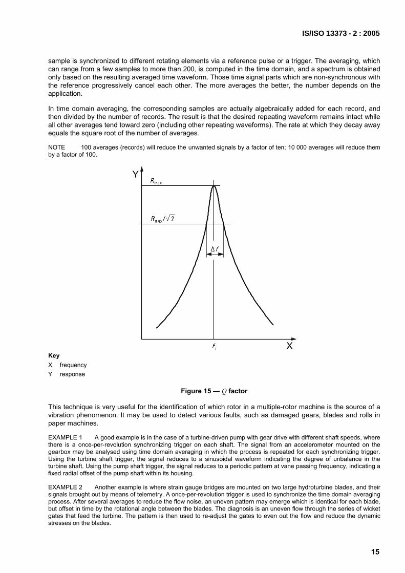
sample is synchronized to different rotating elements via a reference pulse or a trigger. The averaging, which can range from a few samples to more than 200, is computed in the time domain, and a spectrum is obtained only based on the resulting averaged time waveform. Those time signal parts which are non-synchronous with the reference progressively cancel each other. The more averages the better, the number depends on the application.

In time domain averaging, the corresponding samples are actually algebraically added for each record, and then divided by the number of records. The result is that the desired repeating waveform remains intact while all other averages tend toward zero (including other repeating waveforms). The rate at which they decay away equals the square root of the number of averages.

NOTE 100 averages (records) will reduce the unwanted signals by a factor of ten; 10 000 averages will reduce them by a factor of 100.

Key X frequency Y response

Figure 15 — Q factor

This technique is very useful for the identification of which rotor in a multiple-rotor machine is the source of a vibration phenomenon. It may be used to detect various faults, such as damaged gears, blades and rolls in paper machines.

EXAMPLE 1 A good example is in the case of a turbine-driven pump with gear drive with different shaft speeds, where there is a once-per-revolution synchronizing trigger on each shaft. The signal from an accelerometer mounted on the gearbox may be analysed using time domain averaging in which the process is repeated for each synchronizing trigger. Using the turbine shaft trigger, the signal reduces to a sinusoidal waveform indicating the degree of unbalance in the turbine shaft. Using the pump shaft trigger, the signal reduces to a periodic pattern at vane passing frequency, indicating a fixed radial offset of the pump shaft within its housing.

EXAMPLE 2 Another example is where strain gauge bridges are mounted on two large hydroturbine blades, and their signals brought out by means of telemetry. A once-per-revolution trigger is used to synchronize the time domain averaging process. After several averages to reduce the flow noise, an uneven pattern may emerge which is identical for each blade, but offset in time by the rotational angle between the blades. The diagnosis is an uneven flow through the series of wicket gates that feed the turbine. The pattern is then used to re-adjust the gates to even out the flow and reduce the dynamic stresses on the blades.

IS/ISO 13373 - 2 : 2005

15

16

Although very effective, time domain averaging, by its very nature, cannot show asynchronous events such as antifriction bearing faults.

The averaging of complex frequency spectra of successive realizations normally requires a steady-state vibration condition. If there is an unsteady excitation frequency or a changing rotational speed, the simple time domain averaging does not apply. Instead of this, the signal needs to be sampled in constant intervals of the exciting process (e.g. equidistant rotor angle intervals or other positions; this can be done by means of an encoder). The result of the succeeding frequency transformation is an ordering spectrum instead of a frequency spectrum. For impulse response signals, averaging may be executed in the time domain by event triggering, e.g. a trigger tuned by the excitation impulse.

The source of the trigger is not limited to rotating equipment. Other applications, for instance, are paper machine belts, conveyor belts, etc. In addition, the source of the signal is not limited to vibration. It may be a process signal related to the machine in question that can identify a malfunction or a process parameter that should be monitored for fault development. A frequency multiplier may also be used instead of triggering from different shafts, e.g. in the case of multiple shafts such as in a gear box.

4.3 Frequency domain analysis

4.3.1 General

A great deal of vibration analysis is done in the frequency domain because the various sources of vibration can usually be isolated by the frequencies at which they occur. A single channel analysed in the frequency domain gives a great deal of information, but often it is important to relate vibration to a second channel as either a phase or amplitude reference, or both.

4.3.2 Fourier transform

The basic technique for converting a broadband time trace to discrete frequencies, or frequency bands, is by the application of the Fourier transform (FT), a mathematical technique that identifies the sinusoidal components that make up the total vibration signal, including any mechanical or electrical noise that may be present. This analysis can be realized with the help of a computer and signal processing software, by special devices (which are usually called a Fourier analyser), or by hardware microchips (DSPs). More commonly used in analysers now is a more efficient mathematical routine, the fast Fourier transform (FFT).

The time wave form of a vibration signal is converted into distinct sinusoidal components as a function of frequency by means of the FFT, as shown in Figure 16. There are several important basic factors to take into account when setting up an FFT analyser to convert a time wave form into a meaningful frequency spectrum. There is a relationship between the bandwidth of the frequency lines (or bins), the frequency span and the length of the time trace. In Figure 16, the bandwidth is 2 Hz, which is 100 frequency lines between 0 and 200. These parameters should be chosen to optimize the frequency range of interest.

Due to the effects of aliasing (see 4.3.7), higher frequency components can be falsely identified as lower frequency. Anti-aliasing filters should be used in order to avoid this possibility.

The result of a Fourier transform is a complex spectrum, which can be displayed as

amplitude and phase, or

real and imaginary part

of each frequency component.

From a practical viewpoint, the magnitude spectrum has more information; therefore, the phase spectrum is mostly ignored.

IS/ISO 13373 - 2 : 2005

Key X frequency, Hz Y amplitude

Figure 16 — Magnitude frequency spectrum

4.3.3 Leakage and windowing

When sampling a waveform, leakage can occur if the sample contains a non-integral number of cycles. The result is smearing of frequency domain peaks because the sample inaccurately represents the waveform from which it was taken. A window function reduces these errors by correcting for this leakage. The Hanning window does an acceptable job for sine waves that are periodic and non-periodic as time records. Although the Hanning window is most commonly used, there are other types of windows that are available and may be used to enhance the signal.

For transient events a Uniform (rectangular) window produces better results. The Hamming window gives a narrower spectral peak than the Hanning window at higher levels, in exchange for flaring skirts further down. The Blackman window, and its derivatives Blackman Exact and Blackman Harris, give a wider peak than the Hanning, but with even lower skirts. The Flat Top window can improve amplitude accuracy over the Hanning window at the expense of being able to resolve small signals that are closely spaced to large ones in the frequency domain. It gives the widest peak, with skirts equivalent to the Hanning, but the top of the peak is flattest for the most accurate level readings with changing frequencies. By correcting sampling bias, windows improve asynchronous waveform plots such as spectrum, cascade and waterfall. The Flat Top window can also be used for calibration.

NOTE Time domain windows for Fourier Transform analysis are described in ISO 18431-2.

4.3.4 Frequency resolution

The mathematics of an FFT requires that the frequency span of interest be divided into a finite number of sections, and the amplitude of vibration within each section is displayed as a vertical line, sometimes referred to as a “baseband” spectrum. The number of sections is referred to as the number of lines of resolution (LOR),

IS/ISO 13373 - 2 : 2005

17

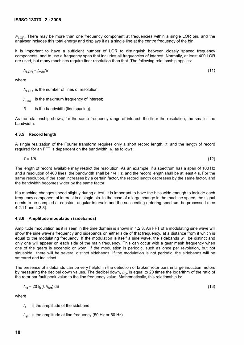
18

NLOR. There may be more than one frequency component at frequencies within a single LOR bin, and the analyser includes this total energy and displays it as a single line at the centre frequency of the bin.

It is important to have a sufficient number of LOR to distinguish between closely spaced frequency components, and to use a frequency span that includes all frequencies of interest. Normally, at least 400 LOR are used, but many machines require finer resolution than that. The following relationship applies:

NLOR = fmax/B (11)

where

NLOR is the number of lines of resolution;

fmax is the maximum frequency of interest;

B is the bandwidth (line spacing).

As the relationship shows, for the same frequency range of interest, the finer the resolution, the smaller the bandwidth.

4.3.5 Record length

A single realization of the Fourier transform requires only a short record length, T, and the length of record required for an FFT is dependent on the bandwidth, B, as follows:

T = 1/B (12)

The length of record available may restrict the resolution. As an example, if a spectrum has a span of 100 Hz and a resolution of 400 lines, the bandwidth shall be 1/4 Hz, and the record length shall be at least 4 s. For the same resolution, if the span increases by a certain factor, the record length decreases by the same factor, and the bandwidth becomes wider by the same factor.

If a machine changes speed slightly during a test, it is important to have the bins wide enough to include each frequency component of interest in a single bin. In the case of a large change in the machine speed, the signal needs to be sampled at constant angular intervals and the succeeding ordering spectrum be processed (see 4.2.11 and 4.3.8).

4.3.6 Amplitude modulation (sidebands)

Amplitude modulation as it is seen in the time domain is shown in 4.2.3. An FFT of a modulating sine wave will show the sine wave’s frequency and sidebands on either side of that frequency, at a distance from it which is equal to the modulating frequency. If the modulation is itself a sine wave, the sidebands will be distinct and only one will appear on each side of the main frequency. This can occur with a gear mesh frequency when one of the gears is eccentric or worn. If the modulation is periodic, such as once per revolution, but not sinusoidal, there will be several distinct sidebands. If the modulation is not periodic, the sidebands will be smeared and indistinct.

The presence of sidebands can be very helpful in the detection of broken rotor bars in large induction motors by measuring the decibel down values. The decibel down, LD, is equal to 20 times the logarithm of the ratio of the rotor bar fault peak value to the line frequency value. Mathematically, this relationship is:

LD = 20 lg(l1/lref) dB (13)

where

l1 is the amplitude of the sideband;

lref is the amplitude at line frequency (50 Hz or 60 Hz).

IS/ISO 13373 - 2 : 2005

As shown in Figure 17, the spectrum for a motor with no problems consists of a clear peak at the line frequency and sidebands equally spaced on either side. The magnitude of the sidebands may be over 60 dB down from the magnitude of the line frequency (60 Hz in this case).

Key X frequency, Hz Y magnitude

Figure 17 — Motor with no problems

Figure 18 is the spectrum for a motor with a fault. In this case, there is a distinct peak at line frequency and elevated sidebands at the rotor bar fault frequencies.

Key X frequency, Hz Y magnitude

Figure 18 — Motor with a fault

IS/ISO 13373 - 2 : 2005

19

20

It can be noted that the structure of the sidebands in the frequency domain has the same information as the envelope spectrum in the time domain.

4.3.7 Aliasing

Aliasing is a false representation of a frequency that can result when the sampling rate of a digital analyser is too low to describe that frequency adequately. It is much the same as when a point on a disc appears fixed if the sampling frequency from a strobe is exactly coincident with the disc rotational frequency. However, if the frequencies are not exactly synchronized, the disc will appear to be rotating slowly. Similarly, if a sine wave is sampled too slowly, it will appear to be a lower frequency. This is eliminated by low-pass filtering the signal before sampling to ensure that it contains no frequency components above half the sampling frequency. This is clearly presented in Figure 19. By comparing the frequency of the high-frequency sine wave and the sampling interval, it can be shown that the sampling frequency is lower than one-half the signal frequency. Therefore, the dotted low-frequency signal will be analysed as an aliasing signal instead of the actually measured one. This is why the sampled amplitudes (the marked joint points in both curves) correspond to the measured high-frequency signal, as well as to the low-frequency aliasing signal.

When the sampling rate is set exactly at two times the maximum expected frequency, this is known as the Nyquist frequency. In practice, most sampling rates are set at greater than two times the maximum frequency (about 2,56 times) to allow for a low-pass filter without a sharp cut-off.

Digital analysers today use anti-aliasing filters that remove all frequencies above 40 % of the sampling rate, before the time data are sampled and converted to digital data; therefore, with most digital analysers, aliasing is no longer a problem. However, the analyst should confirm this before analysing the data.

Key X time Y excitation

a 3/rev excitation. b 13/rev excitation. c 3 and 13 excitation.

Figure 19 — Aliasing

IS/ISO 13373 - 2 : 2005

4.3.8 Synchronous sampling

Rather than sampling at a fixed rate with respect to time, an external signal may be used in many analysers to control the sampling rate. Normally, the sampling rate will be some multiple of the external signal frequency. This is most often used with rotating machinery, where a revolution marker is used to determine the sample rate. The sample rate would be greater than two times the highest-order vibration of interest. There are four major advantages to this procedure, as follows.

a) If the speed of the machine changes, most frequency components which are related to the rotational frequency (blade, vane, gear mesh, etc.) will stay in the same frequency bin, rather than spreading the energy over more than one bin.

b) All orders of vibration are in the centre of a frequency bin where its amplitude is measured more accurately.

c) It is possible to average the series of digitized measuring values without consideration of changes in the rotational speed.

d) All orders of vibration will maintain the same phase angle with respect to the external signal. This means that the spectra can be averaged vectorially, reinforcing the pertinent orders of vibration, but causing other signals not associated with that rotational speed, including most noise signals, to average to zero.

The result of the Fourier transform of a synchronously sampled signal is the ordering spectrum X(n). The order n = 1 corresponds with one vibration period per one rotor revolution.

It is noted that digital order tracking is an approach used in practice (see 4.6).

When performing synchronous averaging, care should also be taken to avoid averaging out any non-harmonic signals of significance (e.g. bearing instability).

4.3.9 Spectrum averaging

Depending on the component frequencies of the signal, a single FFT requires only a fraction of a second or a few seconds of record. However, a modulating signal may require a longer time period to establish a stable average amplitude. Therefore, averaging successive FFTs is a very important function of analysers. If only one channel is available, the absolute amplitudes in each bin are averaged without regard to the phase. Averaging of the complete spectrum (real and imaginary part) requires a synchronization of each successive spectrum by a process-dependent trigger signal.

There are other averaging techniques that may be applied, such as frequency domain averaging, but this technique quickly becomes very complicated and is therefore used only for special applications.

Many analysers do, however, perform exponential averaging, which weights the FFTs with an exponentially increasing function, thereby weighting the signal in favour of the most recently recorded data. This technique is often used for studies of transient vibration in which the amplitudes are exponentially decreasing.

Another type of averaging found on analysers is peak averaging. This finds the maximum amplitude during a given time period of all the FFTs in each of the frequency bins and displays those peaks. Note that each peak is the average amplitude within its own time record.

4.3.10 Logarithmic plots (with dB references)

With vibration records, there are usually many frequency components with greatly varying amplitudes. Many of the components with small amplitudes are important but, when plotted on a linear scale, can hardly be seen. A logarithmic plot, which compresses the large components and enlarges the small, shows all the significant components, as well as the level of noise present. The amplitude, X, is plotted as level, L, in decibels:

L = 20 lg(X/Xref) dB (14)

where Xref is a reference value.

IS/ISO 13373 - 2 : 2005

21

22

Sometimes the frequency axis is also displayed in a logarithmic scale for better recognition, or for separation of the low-frequency components. On the abscissa, the decibel unit is not used (see 4.7).

Differences in decibels are equivalent to ratios, examples of which are shown in Table 1.

Table 1 — Differences in decibels and equivalent ratios

Difference dB Ratio

0 1

6 2

20 10

26 20

40 100

60 1 000

Ratios smaller than one are reflected by negative decibel values, e.g. a ratio of 1/2 is −6 dB.

Reference values for logarithmic levels are specified in ISO 1683, except for displacement. For vibration analyses, the values given in Table 2 may be used.

Table 2 — Reference values for logarithmic levels

Quantity Reference value

Acceleration 10−6 m/s2

Velocity 10−9 m/s

Displacement 10−12 m

Power 10−12 W

4.3.11 Zoom analysis

Often frequency components are too close together to distinguish between them on a normal FFT, which generally consists of 400 lines (base band); however others exist. Some analysers have higher resolution, but often zoom spectra are used to get better resolution. A zoom analysis creates a spectrum with a frequency scale that does not start at zero but at another free eligible frequency, so that the selected number of lines are utilized to expand the frequency range of interest. The bandwidth is correspondingly narrower; however, the record length will still be related to the bandwidth. One problem in using the zoom spectra is that the frequencies must be more stable because of the narrower bandwidth.

An example of the use of zoom spectra is in gear fault analysis. When applied, a fault will result in sidebands of the gear mesh frequency and the spacing of the sidebands will indicate the faulted wheel. A similar zoom approach may also be useful to identify faults in rolling element bearings. Figure 20 shows the advantages of performing zoom analysis. Note that the frequency components not visible in the original zoomed spectrum are now visible.

IS/ISO 13373 - 2 : 2005

Key a Section of original spectrum. b Higher resolution translated spectrum.

Figure 20 — Zoom analysis

4.3.12 Differentiation and integration

Differentiation and integration are important in vibration analysis when signals shall be converted between displacement, velocity and acceleration. For rotating machinery, the vibration signal is often dominated by the synchronous component, and can therefore be harmonic motion. The following formulae then take on the following appearance in the time domain (see also 3.3.2):

displacement: ˆ sinx x tω= ⋅ (15)

velocity: ˆ ˆcos cosv x t v tω ω ω= ⋅ = ⋅ (16)

acceleration: 2 ˆ ˆ ˆsin sin sina x t v t a tω ω ω ω ω= − ⋅ = − ⋅ = − ⋅ (17)

and

acceleration: ˆ sina a tω= ⋅ (18)

velocity: ˆ ˆcos cosav t v tω ωω

= − ⋅ = − ⋅ (19)

displacement: 2ˆ ˆ ˆsin sin sina vx t t x tω ω ω

ωω= − ⋅ = − ⋅ = − ⋅ (20)

The displacement lags the velocity by 90°, and the velocity lags the acceleration by 90°. To convert between quantities in the frequency domain, both differentiation and integration may be carried out by dividing or multiplying, respectively, each component by its angular frequency. Most analysers include these functions for the frequency domain.

It is stressed that to utilize accurately the integration and differentiation formulae, the vibration signal must be predominantly synchronous. It is necessary to check to determine if the 1 × component is greater than 90 % of the unfiltered, or direct, component. Otherwise, each spectral frequency shall be converted separately.

IS/ISO 13373 - 2 : 2005

23

24

4.4 Display of results during operational changes

4.4.1 Amplitude and phase (Bode plot)

When a harmonic vibration signal is expressed in terms of an amplitude and phase, a second signal is required as a reference for the phase. It may be a shaft revolution marker, the vibration at a different location or direction, a measured force or some other appropriate reference. The frequency(ies) of the second signal shall be considered in relation to the frequencies of interest. For example, a shaft revolution marker could be used as a phase reference for rotational frequency or any of the higher harmonics of rotational frequency.

The phase may be expressed as between 0 and 360°, or ± 180°.

When the two signals represent different quantities (e.g. force, velocity, acceleration), care shall be taken to interpret the physical significance properly. Note that, for any sine wave, the displacement lags the velocity by 90°, and the velocity lags the acceleration by 90°. Very often, signal-conditioning equipment changes the phases of the signals, and differences between channels shall be compensated for.

The amplitude and phase of a sine wave may be plotted as a function of time. However, when the amplitude and phase of a machine vibration is plotted against the machine speed, it becomes a Bode plot, as shown in Figure 21.

Key X speed Y amplitude Y′ phase, degrees

a Resonance.

Figure 21 — Amplitude and phase (Bode plot)

4.4.2 Polar diagram (Nyquist diagram)

In a polar diagram, each point represents an amplitude/phase vector for a discrete frequency as shown in Figure 22. If the diagram includes several vectors for different rotating speeds, or other parameters, by showing only the connecting line between their tips, it is known as a Nyquist diagram.

A polar diagram shall have a phase reference, such as a shaft revolution marker, that indicates each 360° rotation of the shaft. Polar diagram (and/or Bode plots) are used to identify accurately the location (speed) of any resonances of the rotor/bearing/support system.

IS/ISO 13373 - 2 : 2005

NOTE The parameter is the rotor speed (r/min).

Figure 22 — Polar diagram (Nyquist diagram)

4.4.3 Cascade (waterfall) diagram

The cascade or waterfall diagram provides a simple comparison of several frequency analyses. It is a three-dimensional form of spectra display that clearly shows vibration signal changes related to another parameter (such as speed, load, temperature, time) taken for specified parameter values, such as time.

The sample cascade spectrum of Figure 23 is an overall picture of many vibration spectra for a machine in the start-up/coast-down region. Normally, the cascade spectrum display provides frequency (Hz or orders) versus machine rotational speed and vibration amplitude of the discrete frequency components. In some cases, however, the machine speed may be substituted by another variable (e.g. time, load), in which case it is then called a waterfall diagram. When using machine speed for this display, it is necessary to record a rotor speed/phase reference signal.

The cascade spectrum of Figure 24 shows the fundamental rotor speed (1 ×) and any other significant harmonic. It also shows the presence of rotor critical speeds, if in the transient speed range.

IS/ISO 13373 - 2 : 2005

25

26

Key X frequency, Hz Y speed, r/min Y′ amplitude

Figure 23 — Waterfall (cascade) plot

Key X frequency, Hz Y time of day Y′ speed, r/min Y′′ amplitude

Figure 24 — Turbine cascade plot

IS/ISO 13373 - 2 : 2005

The shape of the plot will vary, depending on the type of machine and the operation. For example, Figure 24 is a cascade plot of a 3 000 r/min (50 Hz) steam turbine during start-up and coast-down.

For time-dependent spectra, an alternative representation is to use a spectrogram. This is a two-dimensional presentation of a cascade plot which shows speed changes over time but indicates the amplitude height by different colours or intensitives of grey shading (see Figure 25).

NOTE The example in Figure 25 shows another machine than that in Figures 23 and 24.

Key X frequency, Hz Y time, s Y′ amplitude, m/s2 (indicated by grey shading)

Figure 25 — Two-dimensional spectrogram

4.4.4 Campbell diagram

The Campbell diagram (see Figure 26) is a special kind of cascade diagram. It relates the actual frequencies of individual frequency components, such as blade, vane, gear mesh, to the rotational speed. Vibration amplitude can be plotted in the third dimension, so it is represented by the height of the corresponding bars. Campbell diagrams are especially useful for identifying self-excited natural vibration.

IS/ISO 13373 - 2 : 2005

27

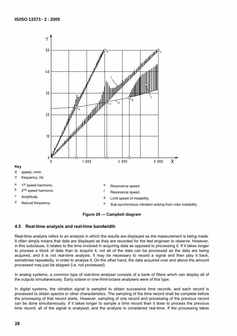
28

Key X speed, r/min Y frequency, Hz

a 1st speed harmonic. b 2nd speed harmonic. c Amplitude. d Natural frequency.

e Resonance speed. f Resonance speed. g Limit speed of instability. h Sub-synchronous vibration arising from rotor instability.

Figure 26 — Campbell diagram

4.5 Real-time analysis and real-time bandwidth

Real-time analysis refers to an analysis in which the results are displayed as the measurement is being made. It often simply means that data are displayed as they are recorded for the test engineer to observe. However, in this subclause, it relates to the time involved in acquiring data as opposed to processing it. If it takes longer to process a block of data than to acquire it, not all of the data can be processed as the data are being acquired, and it is not real-time analysis. It may be necessary to record a signal and then play it back, sometimes repeatedly, in order to analyse it. On the other hand, the data acquired over and above the amount processed may just be skipped (i.e. not processed).

In analog systems, a common type of real-time analyser consists of a bank of filters which can display all of the outputs simultaneously. Early octave or one-third-octave analysers were of this type.

In digital systems, the vibration signal is sampled to obtain successive time records, and each record is processed to obtain spectra or other characteristics. The sampling of the time record shall be complete before the processing of that record starts. However, sampling of one record and processing of the previous record can be done simultaneously. If it takes longer to sample a time record than it does to process the previous time record, all of the signal is analysed, and the analysis is considered real-time. If the processing takes

IS/ISO 13373 - 2 : 2005

longer than the sampling, parts of the signal are missed and the analysis is not considered real-time. Different analysers process data at different speeds, and the maximum frequency span at which data are processed real-time is the real-time bandwidth.

For most machinery measurements at a constant speed, real-time analysis is not required. However, for transient events, including start-ups and coast-downs, a real-time bandwidth that is too small may result in missing relevant data. The most common technique to avoid this is to record the entire event and then play it back at a lower speed to analyse it.

4.6 Order tracking (analog and digital)

When obtaining frequency spectra from machines, if the speed of the machine varies, it may be difficult to obtain meaningful averages because the energy from a particular order may be reflected in more than one frequency bin, and at lower levels than if the speed were constant. By controlling the sampling rate according to the speed of the machine by means of external sampling (see 4.3.8), all of the energy in a particular order of vibration will be reflected in just one frequency bin. This is normally accomplished by using a once-per-revolution signal as input to a dynamic signal analyser and is called order tracking.

Order tracking was first done with a tracking filter for alias protection, and a ratio synthesizer to change the r/min signal to a sampling frequency (2,56 times the highest order of interest). Noise and accuracy concerns, along with restrictions on the rates of change in r/min, led to computed order tracking, which digitizes the process.

In computed order tracking, both the vibration signal and the r/min signal are digitized with fixed sampling rates. The r/min signal is used to establish the sampling rate for each revolution, and the vibration signal is interpolated and re-sampled at the appropriate intervals for the order analysis to establish a stepwise changing individual sampling frequency for each revolution or, by means of polynomial interpolation, a continuously changing sampling frequency can also be generated.

As indicated in 4.3.8, this process has two additional advantages over time-based sampling. All the energy for each order is in the middle of the window for each bin, eliminating the error caused by not being in the middle, which can be up to 15 %.

The other advantage is that it is possible to obtain averaged records with the rotational angle a “time-axis” now, and also in the case of non-steady rotational frequency, and then to process ordering spectra for only the vibration at orders of the r/min. If vector averages are used, vibration at other frequencies will not have a constant phase with respect to the r/min, and will average to zero. Ordering spectra can be averaged without any smearing of the components.

4.7 Octave and fractional-octave analysis

An octave is another relative term signifying a doubled or halved frequency, depending on whether the frequency is being increased or decreased. For example, one octave above 100 Hz would be 200 Hz, while one octave below 100 Hz would be 50 Hz. Thus, while the decibel is a convenient unit to express amplitude ratios, the octave is a convenient way to express frequency ratios. For improved resolution, octaves can be logarithmically split into fractional octaves (e.g. one-third octaves).

4.8 Cepstrum analysis

The cepstrum analysis technique is the reverse transformation of the logarithmic-arithmetic power spectrum of measured vibration data in the time domain. A cepstrum is displayed in a spectral format with amplitude on the vertical axis and a pseudo time called “quefrency” on the horizontal axis. A cepstrum is a spectrum of a spectrum. A fundamental and its harmonic series are thus reduced to a single component.

A cepstrum is ideally suited to the analysis of complex signals containing multiple harmonic series such as generated by gearboxes or rolling element bearings. The ability to isolate and enhance periodic functions so their relationship can be identified is the major advantage of a cepstrum. See Table 3 for the step-by-step progression in the development of a cepstrum analysis.

IS/ISO 13373 - 2 : 2005

29

30

Table 3 — Processing of cepstrum

Activity Result

Measurement of the time history digitized signal x(t)

FFT of the digitized signal amplitude spectrum X(f)

Square the magnitudes of the components of the amplitude spectrum

power spectrum SXX(f) = X2(f)

Calculate 10 times the logarithm of the power spectrum

10 lg SXX(f) dB

Inverse FFT of 10 lg SXX(f) dB power cepstrum CXX(t)

IS/ISO 13373 - 2 : 2005

5 Other techniques

This part of ISO 13373 presents the most commonly used techniques when carrying out narrowband vibration condition monitoring and vibration diagnostics. However, there are other procedures that when applied to special cases can be very useful for solving particular problems. Some of these advanced techniques are listed below for information:

crest factor,

time history,

auto-correlation function,

cross-correlation function,

kurtosis,

composite or full spectra,

inverse Fourier transform,

high-frequency detection,

intensity methods,

multi-trend analysis (r.m.s. values, frequency components, hours, calendar time, high speed),

peak view analysis,

shock pulse measurements,

wavelets,

vector analysis, and

spike energy.

IS/ISO 13373 - 2 : 2005

31

32

Bibliography

[1] ISO 2041, Vibration and shock — Vocabulary

[2] ISO 2954, Mechanical vibration of rotating and reciprocating machinery — Requirements for instruments for measuring vibration severity

[3] ISO 5348, Mechanical vibration and shock — Mechanical mounting of accelerometers

[4] ISO 7919 (all parts), Mechanical vibration — Evaluation of machine vibration by measurements on rotating shafts

[5] ISO 10816 (all parts), Mechanical vibration — Evaluation of machine vibration by measurements on non- rotating parts

[6] ISO 10817-1, Rotating shaft vibration measuring systems — Part 1: Relative and absolute sensing of radial vibration

[7] ISO 13372, Condition monitoring and diagnostics of machines — Vocabulary

[8] ISO 13373-1, Condition monitoring and diagnostics of machines — Vibration condition monitoring — Part 1: General procedures

[9] ISO 16063-21, Methods for the calibration of vibration and shock transducers — Part 21: Vibration calibration by comparison to a reference transducer

[10] ISO 18431 (all parts), Mechanical vibration and shock — Signal processing

[11] VDI 3839 Blatt 1, Hinweise zur Messung und Interpretation der Schwingungen von Maschinen — Allgemeine Grundlagen (Instructions on measuring and interpreting the vibrations of machine — General principles) (Bilingual edition)

[12] VDI 3841, Schwingungsüberwachung von Maschinen — Erforderliche Messungen (Vibration monitoring of machinery — Necessary measurements) (Bilingual edition)

[13] MITCHELL, J. S. An introduction to machinery analysis and monitoring. Pennwell Publishing, 1993

IS/ISO 13373 - 2 : 2005

Bureau of Indian Standards

BIS is a statutory institution established under the Bureau of Indian Standards Act, 1986 to promoteharmonious development of the activities of standardization, marking and quality certification of goodsand attending to connected matters in the country.

Copyright

BIS has the copyright of all its publications. No part of these publications may be reproduced in any formwithout the prior permission in writing of BIS. This does not preclude the free use, in course of imple-menting the standard, of necessary details, such as symbols and sizes, type or grade designations.Enquiries relating to copyright be addressed to the Director (Publications), BIS.

Review of Indian Standards

Amendments are issued to standards as the need arises on the basis of comments. Standards are alsoreviewed periodically; a standard along with amendments is reaffirmed when such review indicates thatno changes are needed; if the review indicates that changes are needed, it is taken up for revision. Usersof Indian Standards should ascertain that they are in possession of the latest amendments or edition byreferring to the latest issue of ‘BIS Catalogue’ and ‘Standards: Monthly Additions’.

This Indian Standard has been developed from Doc No. : MED 28 (1013).

Amendments Issued Since Publication______________________________________________________________________________________

Amendment No. Date of Issue Text Affected______________________________________________________________________________________

______________________________________________________________________________________

______________________________________________________________________________________

______________________________________________________________________________________

______________________________________________________________________________________

BUREAU OF INDIAN STANDARDSHeadquarters:

Manak Bhavan, 9 Bahadur Shah Zafar Marg, New Delhi 110002Telephones: 2323 0131, 2323 3375, 2323 9402 Website: www.bis.org.in

Regional Offices: Telephones

Central : Manak Bhavan, 9 Bahadur Shah Zafar Marg 2323 7617NEW DELHI 110002 2323 3841

Eastern : 1/14, C.I.T. Scheme VII M, V.I.P. Road, Kankurgachi 2337 8499, 2337 8561KOLKATA 700054 2337 8626, 2337 9120

Northern : SCO 335-336, Sector 34-A, CHANDIGARH 160022 260 3843260 9285

Southern : C.I.T. Campus, IV Cross Road, CHENNAI 600113 2254 1216, 2254 14422254 2519, 2254 2315

Western : Manakalaya, E9 MIDC, Marol, Andheri (East) 2832 9295, 2832 7858MUMBAI 400093 2832 7891, 2832 7892

Branches: AHMEDABAD. BANGALORE. BHOPAL. BHUBANESHWAR. COIMBATORE. DEHRADUN.FARIDABAD. GHAZIABAD. GUWAHATI. HYDERABAD. JAIPUR. KANPUR. LUCKNOW.NAGPUR. PARWANOO. PATNA. PUNE. RAJKOT. THIRUVANATHAPURAM. VISAKHAPATNAM.

K.G. Computers, Ashok Vihar, Delhi

{{

{{{