Hmms Spring2013

8/12/2019 Hmms Spring2013

http://slidepdf.com/reader/full/hmms-spring2013 1/22

Chapter 2

Tagging Problems, and Hidden

Markov Models

(Course notes for NLP by Michael Collins, Columbia University)

2.1 Introduction

In many NLP problems, we would like to model pairs of sequences. Part-of-speech

(POS) tagging is perhaps the earliest, and most famous, example of this type of

problem. In POS tagging our goal is to build a model whose input is a sentence,

for example

the dog saw a cat

and whose output is a tag sequence, for example

D N V D N (2.1)

(here we use D for a determiner, N for noun, and V for verb). The tag sequence is

the same length as the input sentence, and therefore specifies a single tag for each

word in the sentence (in this example D for the, N for dog, V for saw, and so on).

We will use x1 . . . xn to denote the input to the tagging model: we will often

refer to this as a sentence. In the above example we have the length n = 5, and

x1 = the, x2 = dog, x3 = saw, x4 = the, x5 = cat . We will use y1 . . . yn to denote

the output of the tagging model: we will often refer to this as the state sequence ortag sequence. In the above example we have y1 = D, y2 = N, y3 = V, and so on.

This type of problem, where the task is to map a sentence x1 . . . xn to a tag se-

quence y1 . . . yn, is often referred to as a sequence labeling problem, or a tagging

problem.

1



2CHAPTER 2. TAGGING PROBLEMS, AND HIDDEN MARKOV MODELS(COURSE NOTES

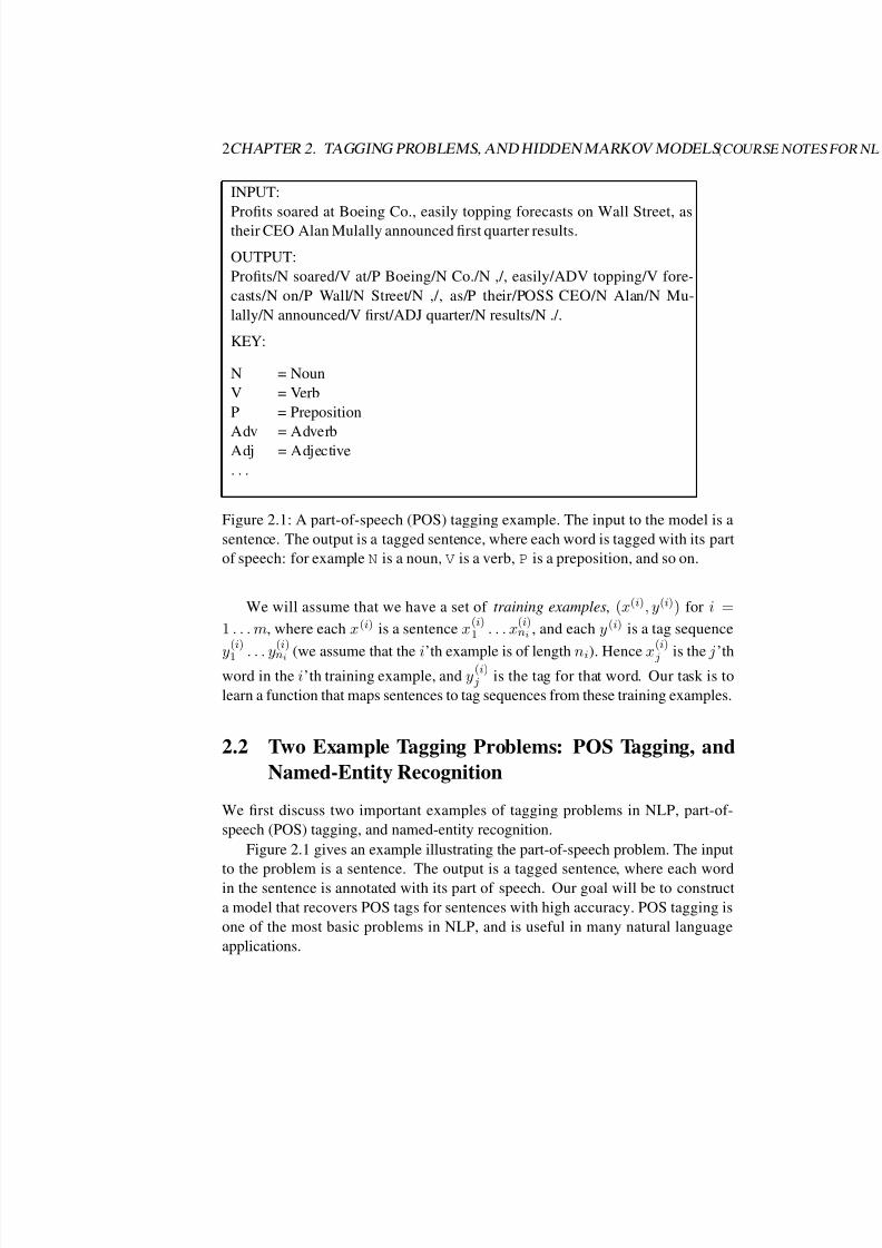
INPUT:

Profits soared at Boeing Co., easily topping forecasts on Wall Street, astheir CEO Alan Mulally announced first quarter results.

OUTPUT:

Profits/N soared/V at/P Boeing/N Co./N ,/, easily/ADV topping/V fore-

casts/N on/P Wall/N Street/N ,/, as/P their/POSS CEO/N Alan/N Mu-

lally/N announced/V first/ADJ quarter/N results/N ./.

KEY:

N = Noun

V = Verb

P = Preposition

Adv = AdverbAdj = Adjective

. . .

Figure 2.1: A part-of-speech (POS) tagging example. The input to the model is a

sentence. The output is a tagged sentence, where each word is tagged with its part

of speech: for example N is a noun, V is a verb, P is a preposition, and so on.

We will assume that we have a set of training examples, (x(i), y(i)) for i =

1 . . .m, where each x(i) is a sentence x(i)1 . . . x

(i)ni , and each y(i) is a tag sequence

y(i)1 . . . y

(i)ni (we assume that the i’th example is of length ni). Hence x

(i) j is the j’th

word in the i’th training example, and y(i) j is the tag for that word. Our task is to

learn a function that maps sentences to tag sequences from these training examples.

2.2 Two Example Tagging Problems: POS Tagging, and

Named-Entity Recognition

We first discuss two important examples of tagging problems in NLP, part-of-

speech (POS) tagging, and named-entity recognition.

Figure 2.1 gives an example illustrating the part-of-speech problem. The input

to the problem is a sentence. The output is a tagged sentence, where each wordin the sentence is annotated with its part of speech. Our goal will be to construct

a model that recovers POS tags for sentences with high accuracy. POS tagging is

one of the most basic problems in NLP, and is useful in many natural language

applications.



2.2. TWO EXAMPLE TAGGING PROBLEMS: POS TAGGING, AND NAMED-ENTITY RECOGNITION

We will assume that we have a set of training examples for the problem: that

is, we have a set of sentences paired with their correct POS tag sequences. As oneexample, the Penn WSJ treebank corpus contains around 1 million words (around

40,000 sentences) annotated with their POS tags. Similar resources are available

in many other languages and genres.

One of the main challenges in POS tagging is ambiguity. Many words in En-

glish can take several possible parts of speech—a similar observation is true for

many other languages. The example sentence in figure 2.1 has several ambiguous

words. For example, the first word in the sentence, profits, is a noun in this context,

but can also be a verb (e.g., in the company profits from its endeavors). The word

topping is a verb in this particular sentence, but can also be a noun (e.g., the top-

ping on the cake). The words forecasts and results are both nouns in the sentence,

but can also be verbs in other contexts. If we look further, we see that quarter is a

noun in this sentence, but it also has a much less frequent usage, as a verb. We can

see from this sentence that there is a surprising amount of ambiguity at the POS

level.

A second challenge is the presence of words that are rare, in particular words

that are not seen in our training examples. Even with say a million words of training

data, there will be many words in new sentences which have not been seen in

training. As one example, words such as Mulally or topping are potentially quite

rare, and may not have been seen in our training examples. It will be important

to develop methods that deal effectively with words which have not been seen in

training data.

In recovering POS tags, it is useful to think of two different sources of informa-

tion. First, individual words have statistical preferences for their part of speech: forexample, quarter can be a noun or a verb, but is more likely to be a noun. Second,

the context has an important effect on the part of speech for a word. In particular,

some sequences of POS tags are much more likely than others. If we consider POS

trigrams, the sequence D N V will be frequent in English (e.g., in the/D dog/N

saw/V . . .), whereas the sequence D V N is much less likely.

Sometimes these two sources of evidence are in conflict: for example, in the

sentence

The trash can is hard to find

the part of speech for can is a noun—however, can can also be a modal verb, and in

fact it is much more frequently seen as a modal verb in English. 1 In this sentence

the context has overridden the tendency for can to be a verb as opposed to a noun.

1There are over 30 uses of the word “can” in this chapter, and if we exclude the example given

above, in every case “can” is used as a modal verb.




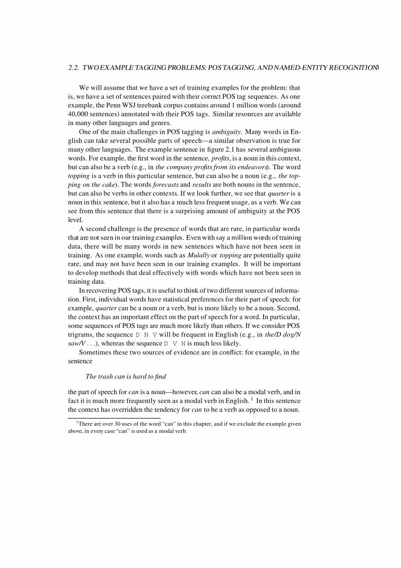
INPUT: Profits soared at Boeing Co., easily topping forecasts on Wall Street, as

their CEO Alan Mulally announced first quarter results.

OUTPUT: Profits soared at [Company Boeing Co.], easily topping forecasts on

[Location Wall Street], as their CEO [Person Alan Mulally] announced first quarter

results.

Figure 2.2: A Named-Entity Recognition Example. The input to the problem is a

sentence. The output is a sentence annotated with named-entities corresponding to

companies, location, and people.

Later in this chapter we will describe models for the tagging problem that take

into account both sources of information—local and contextual—when making

tagging decisions.A second important example tagging problem is named entity recognition. Fig-

ure 2.2 gives an example. For this problem the input is again a sentence. The output

is the sentence with entity-boundaries marked. In this example we assume there

are three possible entity types: PERSON, LOCATION, and COMPANY. The output

in this example identifies Boeing Co. as a company, Wall Street as a location, and

Alan Mulally as a person. Recognising entities such as people, locations and or-

ganizations has many applications, and named-entity recognition has been widely

studied in NLP research.

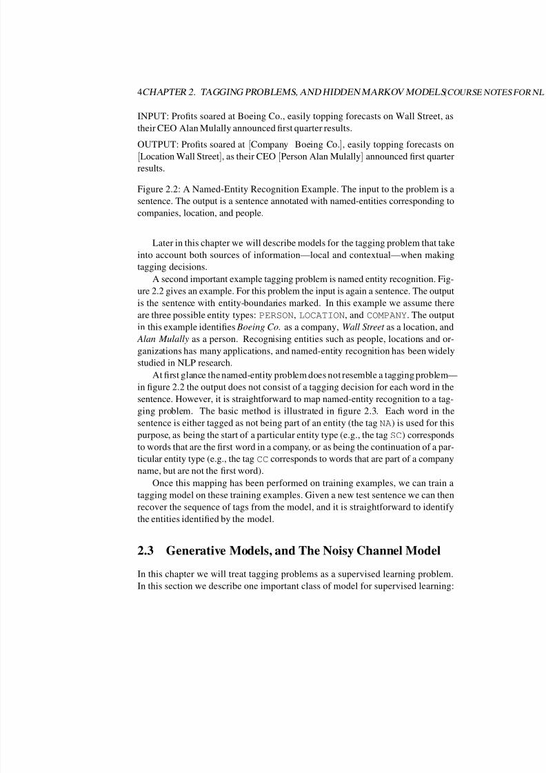
At first glance the named-entity problem does not resemble a tagging problem—

in figure 2.2 the output does not consist of a tagging decision for each word in the

sentence. However, it is straightforward to map named-entity recognition to a tag-

ging problem. The basic method is illustrated in figure 2.3. Each word in the

sentence is either tagged as not being part of an entity (the tag NA) is used for this

purpose, as being the start of a particular entity type (e.g., the tag SC) corresponds

to words that are the first word in a company, or as being the continuation of a par-

ticular entity type (e.g., the tag CC corresponds to words that are part of a company

name, but are not the first word).

Once this mapping has been performed on training examples, we can train a

tagging model on these training examples. Given a new test sentence we can then

recover the sequence of tags from the model, and it is straightforward to identify

the entities identified by the model.

2.3 Generative Models, and The Noisy Channel Model

In this chapter we will treat tagging problems as a supervised learning problem.

In this section we describe one important class of model for supervised learning:



2.3. GENERATIVE MODELS, AND THE NOISY CHANNEL MODEL 5

INPUT: Profits soared at Boeing Co., easily topping forecasts on Wall Street, as

their CEO Alan Mulally announced first quarter results.

OUTPUT: Profits/NA soared/NA at/NA Boeing/SC Co./CC ,/NA easily/NA top-

ping/NA forecasts/NA on/NA Wall/SL Street/CL ,/NA as/NA their/NA CEO/NA

Alan/SP Mulally/CP announced/NA first/NA quarter/NA results/NA ./NA

KEY:

NA = No entity

SC = Start Company

CC = Continue Company

SL = Start Location

CL = Continue Location

. . .

Figure 2.3: Named-Entity Recognition as a Tagging Problem. There are three

entity types: PERSON, LOCATION, and COMPANY. For each entity type we intro-

duce a tag for the start of that entity type, and for the continuation of that entity

type. The tag NA is used for words which are not part of an entity. We can then

represent the named-entity output in figure 2.2 as a sequence of tagging decisions

using this tag set.




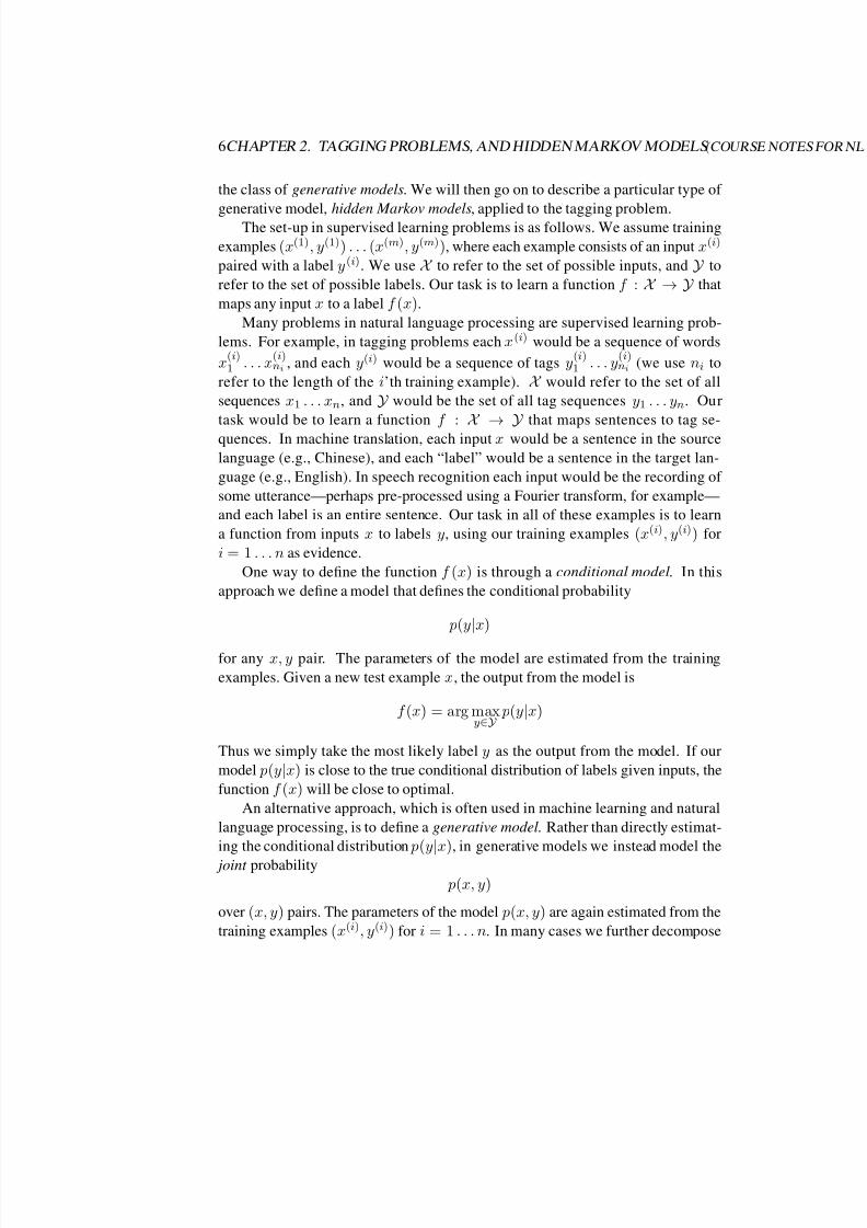
the class of generative models. We will then go on to describe a particular type of

generative model, hidden Markov models, applied to the tagging problem.The set-up in supervised learning problems is as follows. We assume training

examples (x(1), y(1)) . . . (x(m), y(m)), where each example consists of an input x(i)

paired with a label y(i). We use X to refer to the set of possible inputs, and Y to

refer to the set of possible labels. Our task is to learn a function f : X → Y that

maps any input x to a label f (x).

Many problems in natural language processing are supervised learning prob-

lems. For example, in tagging problems each x(i) would be a sequence of words

x(i)1 . . . x

(i)ni , and each y(i) would be a sequence of tags y

(i)1 . . . y

(i)ni (we use ni to

refer to the length of the i’th training example). X would refer to the set of all

sequences x1 . . . xn, and Y would be the set of all tag sequences y1 . . . yn. Our

task would be to learn a function f : X → Y that maps sentences to tag se-

quences. In machine translation, each input x would be a sentence in the source

language (e.g., Chinese), and each “label” would be a sentence in the target lan-

guage (e.g., English). In speech recognition each input would be the recording of

some utterance—perhaps pre-processed using a Fourier transform, for example—

and each label is an entire sentence. Our task in all of these examples is to learn

a function from inputs x to labels y, using our training examples (x(i), y(i)) for

i = 1 . . . n as evidence.

One way to define the function f (x) is through a conditional model. In this

approach we define a model that defines the conditional probability

p(y|x)

for any x, y pair. The parameters of the model are estimated from the training

examples. Given a new test example x, the output from the model is

f (x) = arg maxy∈Y

p(y|x)

Thus we simply take the most likely label y as the output from the model. If our

model p(y|x) is close to the true conditional distribution of labels given inputs, the

function f (x) will be close to optimal.

An alternative approach, which is often used in machine learning and natural

language processing, is to define a generative model. Rather than directly estimat-

ing the conditional distribution p(y|x), in generative models we instead model the

joint probability

p(x, y)

over (x, y) pairs. The parameters of the model p(x, y) are again estimated from the

training examples (x(i), y(i)) for i = 1 . . . n. In many cases we further decompose



2.3. GENERATIVE MODELS, AND THE NOISY CHANNEL MODEL 7

the probability p(x, y) as follows:

p(x, y) = p(y) p(x|y) (2.2)

and then estimate the models for p(y) and p(x|y) separately. These two model

components have the following interpretations:

• p(y) is a prior probability distribution over labels y.

• p(x|y) is the probability of generating the input x, given that the underlying

label is y.

We will see that in many cases it is very convenient to decompose models in this

way; for example, the classical approach to speech recognition is based on this type

of decomposition.

Given a generative model, we can use Bayes rule to derive the conditional

probability p(y|x) for any (x, y) pair:

p(y|x) = p(y) p(x|y)

p(x)

where

p(x) =

y∈Y

p(x, y) =

y∈Y

p(y) p(x|y)

Thus the joint model is quite versatile, in that we can also derive the probabilities

p(x

) and p

(y

|x

).

We use Bayes rule directly in applying the joint model to a new test example.

Given an input x, the output of our model, f (x), can be derived as follows:

f (x) = arg m axy

p(y|x)

= arg maxy

p(y) p(x|y)

p(x) (2.3)

= arg maxy

p(y) p(x|y) (2.4)

Eq. 2.3 follows by Bayes rule. Eq. 2.4 follows because the denominator, p(x),

does not depend on y , and hence does not affect the arg max. This is convenient,

because it means that we do not need to calculate p(x), which can be an expensiveoperation.

Models that decompose a joint probability into into terms p(y) and p(x|y) are

often called noisy-channel models. Intuitively, when we see a test example x, we

assume that has been generated in two steps: first, a label y has been chosen with




probability p(y); second, the example x has been generated from the distribution

p(x|y). The model p(x|y) can be interpreted as a “channel” which takes a label yas its input, and corrupts it to produce x as its output. Our task is to find the most

likely label y, given that we observe x.

In summary:

• Our task is to learn a function from inputs x to labels y = f (x). We assume

training examples (x(i), y(i)) for i = 1 . . . n.

• In the noisy channel approach, we use the training examples to estimate

models p(y) and p(x|y). These models define a joint (generative) model

p(x, y) = p(y) p(x|y)

• Given a new test example x, we predict the label

f (x) = arg maxy∈Y

p(y) p(x|y)

Finding the output f (x) for an input x is often referred to as the decoding

problem.

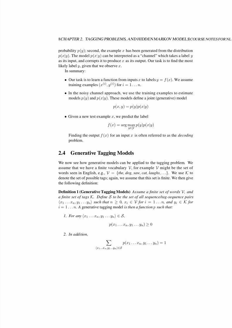
2.4 Generative Tagging Models

We now see how generative models can be applied to the tagging problem. We

assume that we have a finite vocabulary V , for example V might be the set of

words seen in English, e.g., V = {the, dog, saw, cat, laughs, . . .}. We use K to

denote the set of possible tags; again, we assume that this set is finite. We then give

the following definition:

Definition 1 (Generative Tagging Models) Assume a finite set of words V , and

a finite set of tags K. Define S to be the set of all sequence/tag-sequence pairs

x1 . . . xn, y1 . . . yn such that n ≥ 0 , xi ∈ V for i = 1 . . . n , and yi ∈ K for

i = 1 . . . n. A generative tagging model is then a function p such that:

1. For any x1 . . . xn, y1 . . . yn ∈ S ,

p(x1 . . . xn, y1 . . . yn) ≥ 0

2. In addition,

x1...xn,y1...yn∈S

p(x1 . . . xn, y1 . . . yn) = 1



2.5. TRIGRAM HIDDEN MARKOV MODELS (TRIGRAM HMMS) 9

Hence p(x1 . . . xn, y1 . . . yn) is a probability distribution over pairs of sequences

(i.e., a probability distribution over the set S ).Given a generative tagging model, the function from sentences x1 . . . xn to tag

sequences y1 . . . yn is defined as

f (x1 . . . xn) = arg maxy1...yn

p(x1 . . . xn, y1 . . . yn)

where the arg max is taken over all sequences y1 . . . yn such that yi ∈ K for

i ∈ {1 . . . n}. Thus for any input x1 . . . xn , we take the highest probability tag

sequence as the output from the model.

Having introduced generative tagging models, there are three critical questions:

• How we define a generative tagging model p(x1 . . . xn, y1 . . . yn)?

• How do we estimate the parameters of the model from training examples?

• How do we efficiently find

arg maxy1...yn

p(x1 . . . xn, y1 . . . yn)

for any input x1 . . . xn?

The next section describes how trigram hidden Markov models can be used to

answer these three questions.

2.5 Trigram Hidden Markov Models (Trigram HMMs)

In this section we describe an important type of generative tagging model, a trigram

hidden Markov model, describe how the parameters of the model can be estimated

from training examples, and describe how the most likely sequence of tags can be

found for any sentence.

2.5.1 Definition of Trigram HMMs

We now give a formal definition of trigram hidden Markov models (trigram HMMs).

The next section shows how this model form is derived, and gives some intuition

behind the model.

Definition 2 (Trigram Hidden Markov Model (Trigram HMM)) A trigram HMM

consists of a finite set V of possible words, and a finite set K of possible tags, to-

gether with the following parameters:



10CHAPTER 2. TAGGING PROBLEMS, AND HIDDEN MARKOV MODELS(COURSE NOTE

• A parameter

q (s|u, v)

for any trigram (u,v,s) such that s ∈ K ∪ {STOP} , and u, v ∈ K ∪ {*}.

The value for q (s|u, v) can be interpreted as the probability of seeing the tag

s immediately after the bigram of tags (u, v).

• A parameter

e(x|s)

for any x ∈ V , s ∈ K. The value for e(x|s) can be interpreted as the

probability of seeing observation x paired with state s.

Define S to be the set of all sequence/tag-sequence pairs x1 . . . xn, y1 . . . yn+1such that n ≥ 0 , xi ∈ V for i = 1 . . . n , yi ∈ K for i = 1 . . . n , and yn+1 = STOP.

We then define the probability for any x1 . . . xn, y1 . . . yn+1 ∈ S as

p(x1 . . . xn, y1 . . . yn+1) =n+1

i=1

q (yi|yi−2, yi−1)n

i=1

e(xi|yi)

where we have assumed that y0 = y−1 = *.

As one example, if we have n = 3, x1 . . . x3 equal to the sentence the dog

laughs, and y1 . . . y4 equal to the tag sequence D N V STOP, then

p(x1 . . . xn, y1 . . . yn+1) = q (D|∗, ∗) × q (N|∗,D) × q (V|D, N) × q (STOP|N,V)

×e(the|D) × e(dog|N) × e(laughs|V)

Note that this model form is a noisy-channel model. The quantity

q (D|∗, ∗) × q (N|∗, D) × q (V|D,N) × q (STOP|N, V)

is the prior probability of seeing the tag sequence D N V STOP, where we have

used a second-order Markov model (a trigram model), very similar to the language

models we derived in the previous lecture. The quantity

e(the|D) × e(dog|N) × e(laughs|V)

can be interpreted as the conditional probability p(the dog laughs|D N V STOP):

that is, the conditional probability p(x|y) where x is the sentence the dog laughs,

and y is the tag sequence D N V STOP.




2.5.2 Independence Assumptions in Trigram HMMs

We now describe how the form for trigram HMMs can be derived: in particular, we

describe the independence assumptions that are made in the model. Consider a pair

of sequences of random variables X 1 . . . X n, and Y 1 . . . Y n, where n is the length

of the sequences. We assume that each X i can take any value in a finite set V of

words. For example, V might be a set of possible words in English, for example

V = {the, dog, saw, cat, laughs, . . .}. Each Y i can take any value in a finite set Kof possible tags. For example, K might be the set of possible part-of-speech tags

for English, e.g. K = {D,N,V, . . .}.

The lengthn is itself a random variable—it can vary across different sentences—

but we will use a similar technique to the method used for modeling variable-length

Markov processes (see chapter ??).

Our task will be to model the joint probability

P (X 1 = x1 . . . X n = xn, Y 1 = y1 . . . Y n = yn)

for any observation sequencex1 . . . xn paired with a state sequencey1 . . . yn, where

each xi is a member of V , and each yi is a member of K.

We will find it convenient to define one additional random variableY n+1, which

always takes the value STOP. This will play a similar role to the STOP symbol seen

for variable-length Markov sequences, as described in the previous lecture notes.

The key idea in hidden Markov models is the following definition:

P (X 1 = x1 . . . X n = xn, Y 1 = y1 . . . Y n+1 = yn+1)

=

n+1

i=1

P (Y i = yi|Y i−2 = yi−2, Y i−1 = yi−1)

n

i=1

P (X i = xi|Y i = yi)(2.5)

where we have assumed that y0 = y−1 = *, where * is a special start symbol.

Note the similarity to our definition of trigram HMMs. In trigram HMMs we

have made the assumption that the joint probability factorizes as in Eq. 2.5, and in

addition we have assumed that for any i, for any values of yi−2, yi−1, yi,

P (Y i = yi|Y i−2 = yi−2, Y i−1 = yi−1) = q (yi|yi−2, yi−1)

and that for any value of i, for any values of xi and yi,

P (X i = xi|Y i = yi) = e(xi|yi)

We now describe how Eq. 2.5 is derived, in particular focusing on indepen-

dence assumptions that have been made in the model. First, we can write

P (X 1 = x1 . . . X n = xn, Y 1 = y1 . . . Y n+1 = yn+1)

= P (Y 1 = y1 . . . Y n+1 = yn+1) × P (X 1 = x1 . . . X n = xn|Y 1 = y1 . . . Y n+1 = yn+1)

(2.6)




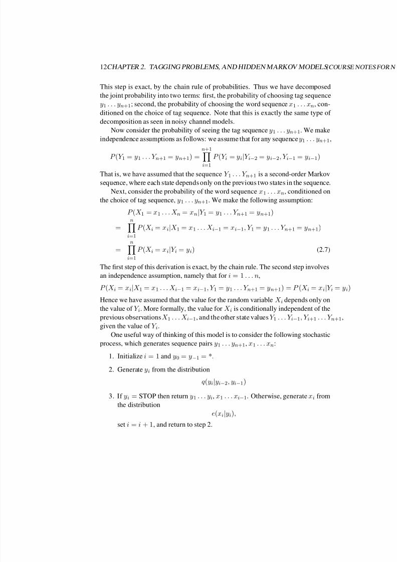
This step is exact, by the chain rule of probabilities. Thus we have decomposed

the joint probability into two terms: first, the probability of choosing tag sequencey1 . . . yn+1; second, the probability of choosing the word sequence x1 . . . xn, con-

ditioned on the choice of tag sequence. Note that this is exactly the same type of

decomposition as seen in noisy channel models.

Now consider the probability of seeing the tag sequence y1 . . . yn+1. We make

independence assumptions as follows: we assume that for any sequence y1 . . . yn+1,

P (Y 1 = y1 . . . Y n+1 = yn+1) =n+1

i=1

P (Y i = yi|Y i−2 = yi−2, Y i−1 = yi−1)

That is, we have assumed that the sequence Y 1 . . . Y n+1 is a second-order Markov

sequence, where each state depends only on the previous two states in the sequence.

Next, consider the probability of the word sequence x1 . . . xn, conditioned on

the choice of tag sequence, y1 . . . yn+1. We make the following assumption:

P (X 1 = x1 . . . X n = xn|Y 1 = y1 . . . Y n+1 = yn+1)

=n

i=1

P (X i = xi|X 1 = x1 . . . X i−1 = xi−1, Y 1 = y1 . . . Y n+1 = yn+1)

=n

i=1

P (X i = xi|Y i = yi) (2.7)

The first step of this derivation is exact, by the chain rule. The second step involves

an independence assumption, namely that for i = 1 . . . n,

P (X i = xi|X 1 = x1 . . . X i−1 = xi−1, Y 1 = y1 . . . Y n+1 = yn+1) = P (X i = xi|Y i = yi)

Hence we have assumed that the value for the random variable X i depends only on

the value of Y i. More formally, the value for X i is conditionally independent of the

previous observationsX 1 . . . X i−1, and the other state valuesY 1 . . . Y i−1, Y i+1 . . . Y n+1,

given the value of Y i.

One useful way of thinking of this model is to consider the following stochastic

process, which generates sequence pairs y1 . . . yn+1, x1 . . . xn:

1. Initialize i = 1 and y0 = y−1 = *.

2. Generate yi from the distribution

q (yi|yi−2, yi−1)

3. If yi = STOP then return y1 . . . yi, x1 . . . xi−1. Otherwise, generate xi from

the distribution

e(xi|yi),

set i = i + 1, and return to step 2.




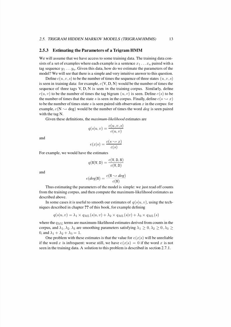
2.5.3 Estimating the Parameters of a Trigram HMM

We will assume that we have access to some training data. The training data con-

sists of a set of examples where each example is a sentence x1 . . . xn paired with a

tag sequence y1 . . . yn. Given this data, how do we estimate the parameters of the

model? We will see that there is a simple and very intuitive answer to this question.

Define c(u,v,s) to be the number of times the sequence of three states (u,v,s)is seen in training data: for example, c(V, D, N) would be the number of times the

sequence of three tags V, D, N is seen in the training corpus. Similarly, define

c(u, v) to be the number of times the tag bigram (u, v) is seen. Define c(s) to be

the number of times that the state s is seen in the corpus. Finally, define c(s x)to be the number of times state s is seen paired sith observation x in the corpus: for

example, c(N dog) would be the number of times the word dog is seen paired

with the tag N.Given these definitions, the maximum-likelihood estimates are

q (s|u, v) = c(u,v,s)

c(u, v)

and

e(x|s) = c(s x)

c(s)

For example, we would have the estimates

q (N|V, D) = c(V,D,N)

c(V,D)

and

e(dog|N) = c(N dog)

c(N)

Thus estimating the parameters of the model is simple: we just read off counts

from the training corpus, and then compute the maximum-likelihood estimates as

described above.

In some cases it is useful to smooth our estimates of q (s|u, v), using the tech-

niques described in chapter ?? of this book, for example defining

q (s|u, v) = λ1 × q ML(s|u, v) + λ2 × q ML(s|v) + λ3 × q ML(s)

where the q ML terms are maximum-likelihood estimates derived from counts in the

corpus, and λ1, λ2, λ3 are smoothing parameters satisfying λ1 ≥ 0, λ2 ≥ 0, λ3 ≥0, and λ1 + λ2 + λ3 = 1.

One problem with these estimates is that the value for e(x|s) will be unreliable

if the word x is infrequent: worse still, we have e(x|s) = 0 if the word x is not

seen in the training data. A solution to this problem is described in section 2.7.1.




2.5.4 Decoding with HMMs: the Viterbi Algorithm

We now turn to the problem of finding the most likely tag sequence for an input

sentence x1 . . . xn. This is the problem of finding

arg maxy1...yn+1

p(x1 . . . xn, y1 . . . yn+1)

where the arg max is taken over all sequences y1 . . . yn+1 such that yi ∈ K for

i = 1 . . . n, and yn+1 = STOP. We assume that p again takes the form

p(x1 . . . xn, y1 . . . yn+1) =n+1

i=1


i=1

e(xi|yi) (2.8)

Recall that we have assumed in this definition that y0

= y−1

= *, and yn+1

=STOP.

The naive, brute force method would be to simply enumerate all possible tag

sequences y1 . . . yn+1, score them under the function p, and take the highest scor-

ing sequence. For example, given the input sentence

the dog barks

and assuming that the set of possible tags is K = {D, N, V}, we would consider all

possible tag sequences:

D D D STOP

D D N STOP

D D V STOP

D N D STOP

D N N STOP

D N V STOP

. . .

and so on. There are 33 = 27 possible sequences in this case.

For longer sentences, however, this method will be hopelessly inefficient. For

an input sentence of length n, there are |K|n possible tag sequences. The expo-

nential growth with respect to the length n means that for any reasonable length

sentence, brute-force search will not be tractable.

The Basic Algorithm

Instead, we will see that we can efficiently find the highest probability tag se-

quence, using a dynamic programming algorithm that is often called the Viterbi




algorithm. The input to the algorithm is a sentence x1 . . . xn. Given this sentence,

for any k ∈ {1 . . . n}, for any sequence y−1, y0, y1, . . . , yk such that yi ∈ K fori = 1 . . . k, and y−1 = y0 = *, we define the function

r(y−1, y0, y1, . . . , yk) =k

i=1

q (yi|yi−2, yi−1)k

i=1

e(xi|yi) (2.9)

This is simply a truncated version of the definition of p in Eq. 2.8, where we just

consider the first k terms. In particular, note that

p(x1 . . . xn, y1 . . . yn+1) = r(*, *, y1, . . . , yn) × q (yn+1|yn−1, yn)

= r(*, *, y1, . . . , yn) × q (STOP|yn−1, yn)

(2.10)

It will be convenient to use Kk for k ∈ {−1 . . . n} to denote the set of allowable

tags at position k in the sequence: more precisely, define

K−1 = Ko = {*}

and

Kk = K for k ∈ {1 . . . n}

Next, for any k ∈ {1 . . . n}, for any u ∈ Kk−1, v ∈ Kk, define S (k,u,v) to be

the set of sequences y−1, y0, y1, . . . , yk such that yk−1 = u, yk = v, and yi ∈ Ki

for i ∈ {−1 . . . k}. Thus S (k,u,v) is the set of all tag sequences of length k,

which end in the tag bigram (u, v

). Define

π(k,u,v) = maxy−1,y0,y1,...,yk∈S (k,u,v)

r(y−1, y0, y1, . . . , yk) (2.11)

Thus π(k,u,v) is the maximum probability for any sequence of length k , ending

in the tag bigram (u, v).

We now observe that we can calculate the π(k,u,v) values for all (k,u,v)efficiently, as follows. First, as a base case define

π(0, *, *) = 1

Next, we give the recursive definition.

Proposition 1 For any k ∈ {1 . . . n} , for any u ∈ Kk−1 and v ∈ Kk , we can use

the following recursive definition:

π(k,u,v) = maxw∈Kk−2

(π(k − 1,w ,u) × q (v|w, u) × e(xk|v)) (2.12)




This definition is recursive because the definition makes use of the π(k − 1,w ,u)

values computed for shorter sequences. This definition will be key to our dynamicprogramming algorithm.

How can we justify this recurrence? Recall that π(k,u,v) is the highest proba-

bility for any sequence y−1 . . . yk ending in the bigram (u, v). Any such sequence

must have yk−2 = w for some state w . The highest probability for any sequence

of length k − 1 ending in the bigram (w, u) is π(k − 1,w ,u), hence the highest

probability for any sequence of length k ending in the trigram (w,u,v) must be

π(k − 1,w ,u) × q (v|w, u) × e(xk|v)

In Eq. 2.12 we simply search over all possible values for w , and return the maxi-

mum.

Our second claim is the following:

Proposition 2

maxy1...yn+1

p(x1 . . . xn, y1 . . . yn+1) = maxu∈Kn−1,v∈Kn

(π(n,u,v) × q (STOP|u, v))

(2.13)

This follows directly from the identity in Eq. 2.10.

Figure 2.4 shows an algorithm that puts these ideas together. The algorithm

takes a sentence x1 . . . xn as input, and returns

maxy1...yn+1

p(x1 . . . xn, y1 . . . yn+1)

as its output. The algorithm first fills in the π(k,u,v) values in using the recursive

definition. It then uses the identity in Eq. 2.13 to calculate the highest probability

for any sequence.

The running time for the algorithm is O(n|K|3), hence it is linear in the length

of the sequence, and cubic in the number of tags.

The Viterbi Algorithm with Backpointers

The algorithm we have just described takes a sentence x1 . . . xn as input, and re-

turns

maxy1...yn+1

p(x1 . . . xn, y1 . . . yn+1)

as its output. However we’d really like an algorithm that returned the highest prob-

ability sequence, that is, an algorithm that returns

arg maxy1...yn+1

p(x1 . . . xn, y1 . . . yn+1)



2.6. SUMMARY 17

Input: a sentence x1 . . . xn, parameters q (s|u, v) and e(x|s).

Definitions: Define K to be the set of possible tags. Define K−1 = K0 = {*}, andKk = K for k = 1 . . . n.

Initialization: Set π(0, *, *) = 1.

Algorithm:

• For k = 1 . . . n,

– For u ∈ Kk−1, v ∈ Kk,


(π(k − 1,w ,u) × q (v|w, u) × e(xk|v))

• Return maxu∈Kn−1,v∈Kn (π(n,u,v) × q (STOP|u, v))

Figure 2.4: The basic Viterbi Algorithm.

for any input sentence x1 . . . xn.

Figure 2.5 shows a modified algorithm that achieves this goal. The key step

is to store backpointer values bp(k,u,v) at each step, which record the previous

state w which leads to the highest scoring sequence ending in (u, v) at position k

(the use of backpointers such as these is very common in dynamic programming

methods). At the end of the algorithm, we unravel the backpointers to find the

highest probability sequence, and then return this sequence. The algorithm again

runs in O(n|K|3) time.

2.6 Summary

We’ve covered a number of important points in this chapter, but the end result is

fairly straightforward: we have derived a complete method for learning a tagger

from a training corpus, and for applying it to new sentences. The main points were

as follows:

• A trigram HMM has parameters q (s|u, v) and e(x|s), and defines the joint

probability of any sentence x1 . . . xn paired with a tag sequence y1 . . . yn+1(where yn+1 = STOP) as

p(x1 . . . xn, y1 . . . yn+1) =n+1

i=1


i=1

e(xi|yi)




Input: a sentence x1 . . . xn, parameters q (s|u, v) and e(x|s).

Definitions: Define K to be the set of possible tags. Define K−1 = K0 = {*}, and

Kk = K for k = 1 . . . n.

Initialization: Set π(0, *, *) = 1.

Algorithm:

• For k = 1 . . . n,

– For u ∈ Kk−1, v ∈ Kk,


(π(k − 1,w ,u) × q (v|w, u) × e(xk|v))

bp(k,u,v) = arg maxw∈Kk−2

(π(k − 1,w ,u) × q (v|w, u) × e(xk|v))

• Set (yn−1, yn) = arg maxu∈Kn−1,v∈Kn (π(n,u,v) × q (STOP|u, v))

• For k = (n − 2) . . . 1,

yk = bp(k + 2, yk+1, yk+2)

• Return the tag sequence y1 . . . yn

Figure 2.5: The Viterbi Algorithm with backpointers.



2.7. ADVANCED MATERIAL 19

• Given a training corpus from which we can derive counts, the maximum-

likelihood estimates for the parameters are

q (s|u, v) = c(u,v,s)

c(u, v)

and

e(x|s) = c(s x)

c(s)

• Given a new sentence x1 . . . xn, and parameters q and e that we have es-

timated from a training corpus, we can find the highest probability tag se-

quence for x1 . . . xn using the algorithm in figure 2.5 (the Viterbi algorithm).

2.7 Advanced Material

2.7.1 Dealing with Unknown Words

Recall that our parameter estimates for the emission probabilities in the HMM are

e(x|s) = c(s x)

c(s)

where c(s x) is the number of times state s is paired with word x in the training

data, and c(s) is the number of times state s is seen in training data.

A major issue with these estimates is that for any word x that is not seen intraining data, e(x|s) will be equal to 0 for all states s. Because of this, for any test

sentence x1 . . . xn that contains some word that is never seen in training data, it is

easily verified that

p(x1 . . . xn, y1 . . . yn+1) = 0

for all tag sequences y1 . . . yn+1. Thus the model will completely fail on the test

sentence. In particular, the arg max in

arg maxy1...yn+1

p(x1 . . . xn, y1 . . . yn+1) = 0

will not be useful: every tag sequence will have the same, maximum score, of 0.

This is an acute problem, because however large our training data, there willinevitably be words in test sentences that are never seen in training data. The

vocabulary size for English, for example, is very large; and new words are always

being encountered in test data. Take for example the sentence used in figures 2.2

and 2.3:




Profits soared at Boeing Co., easily topping forecasts on Wall Street,

as their CEO Alan Mulally announced first quarter results.

In this sentence it is quite likely that the word Mulally has not been seen in training

data. Similarly, topping is a relatively infrequent word in English, and may not

have been seen in training.

In this section we describe a simple but quite effective solution to this problem.

The key idea is to map low frequency words in training data, and in addition words

seen in test data but never seen in training, to a relatively small set of pseudo-words.

For example, we might map the word Mulally to the pseudo-word initCap, the

word 1990 to the pseudo-word fourDigitNum, and so on. Here the pseudo-

word initCap is used for any word whose first letter is a capital, and whose

remaining letters are lower case. The pseudo-word fourDigitNum is used for

any four digit number.

Figure 2.6 shows an example set of pseudo-words, taken from [?], who applied

an HMM tagger to the problem of named entity recognition. This set of pseudo-

words was chosen by hand, and was clearly chosen to preserve some useful infor-

mation about the spelling features of different words: for example capitalization

features of words, and a sub-division into different number types (one of the entity

classes identified in this work was dates, so it is useful to distinguish different types

of numbers, as numbers are often relevant to dates).

Once a mapping from words to pseudo-words is defined we procede as follows.

Define f (x) to be the function that maps a word x to its pseudo-word f (x). We

define some count cut-off γ : a typical value for γ might be γ = 5. For any word

seen in training data less than γ times, we simply replace the word x by its pseudo-word f (x). This mapping is applied to words in both training and test examples:

so words which are never seen in training data, but which are seen in test data, are

also mapped to their pseudo-word. Once this mapping has been performed, we can

estimate the parameters of the HMM in exactly the same way as before, with some

of our words in training data now being pseudo-words. Similarly, we can apply the

Viterbi algorithm for decoding with the model, with some of the words in our input

sentences being pseudo-words.

Mapping low-frequency words to pseudo-words has the effect of “closing the

vocabulary”: with this mapping, every word in test data will be seen at least once

in training data (assuming that each pseudo-word is seen at least once in training,

which is generally the case). Thus we will never have the problem that e(x|s) = 0for some word x in test data. In addition, with a careful choice for the set of

pseudo-words, important information about the spelling of different words will be

preserved. See figure 2.7 for an example sentence before and after the mapping is

applied.



2.7. ADVANCED MATERIAL 21

Word class Example Intuition

twoDigitNum 90 Two digit year

fourDigitNum 1990 Four digit year

containsDigitAndAlpha A8956-67 Product code

containsDigitAndDash 09-96 Date

containsDigitAndSlash 11/9/89 Date

containsDigitAndComma 23,000.00 Monetary amount

containsDigitAndPeriod 1.00 Monetary amount,percentage

othernum 456789 Other number

allCaps BBN Organization

capPeriod M. Person name initial

firstWord first word of sentence no useful capitalization informa-

tion

initCap Sally Capitalized word

lowercase can Uncapitalized word

other , Punctuation marks, all other

words

Figure 2.6: The mapping to pseudo words used by [?] Bikel et. al (1999).

A drawback of the approach is that some care is needed in defining the map-

ping to pseudo-words: and this mapping may vary depending on the task being

considered (for example different mappings might be used for named-entity recog-

nition versus POS tagging). In a later chapter we will see what is arguably a cleanersolution to the problem of low frequency and unknown words, building on ideas

from log-linear models.




Profits/NA soared/NA at/NA Boeing/SC Co./CC ,/NA easily/NA topping/NA fore-

casts/NA on/NA Wall/SL Street/CL ,/NA as/NA their/NA CEO/NA Alan/SP Mu-

lally/CP announced/NA first/NA quarter/NA results/NA ./NA

⇓

firstword /NA soared/NA at/NA initCap /SC Co./CC ,/NA easily/NA

lowercase /NA forecasts/NA on/NA initCap /SL Street/CL ,/NA as/NA

their/NA CEO/NA Alan/SP initCap /CP announced/NA first/NA quarter/NA re-

sults/NA ./NA

NA = No entity

SC = Start Company

CC = Continue Company

SL = Start Location

CL = Continue Location

. . .

Figure 2.7: An example of how the pseudo-word mapping shown in figure 2.6 is

applied to a sentence. Here we are assuming that Profits, Boeing, topping, Wall,

and Mullaly are all seen infrequently enough to be replaced by their pseudo word.

We show the sentence before and after the mapping.

Documents

Hmms Spring2013