Holding Magnetic Field

Abstract

The design of a solenoid to produce the required rotating/holding magnetic field in then-3He experiment is presented. The solenoid is constructed using 19 currents which are15 cm apart from each other. When calculating the magnetic field using the same currentin each coil, it was noticed that the field produced, even it is in the z direction, the shapewas far from the pursued magnetic field; in order to remedy this problem an optimizationwas performed: given that the magnetic field in each point in space is the superpositionof the magnetic fields of each coil in that particular point, therefore it is advantageous towrite the total magnetic field as a vector, which is equal to the product of a magnetic fieldmatrix constructed with the magnetic field of each current times a current vector (themagnetic field vector dimension is n, the number of points where it is desired to establishthe magnetic field, the matrix dimension is n ×m, m is the number of coils, finally thecurrent vector dimension is m). It is easy to see that solving the matrix equation for thecurrent vector, proposing an ideal magnetic field vector, will give the magnitude of thecurrents which would produce this desired magnetic field. Note that n m, consequentlyto obtain the inverse of this matrix, the singular value decomposition technique was used.A weight function was introduced in each side of the matrix equation to help to solvereadily the equation, this weight function is constructed by physical insight: in regionswhere it is of crucial importance to have the proposed magnetic field, the weight functionacquires larger values than it acquires in regions where this importance is smaller. Usingthese techniques, the currents which produce the desired magnetic field were successfullyfound.

1 Introduction

The set up of the n-3He experiment will require some of the technology used in theNPDGamma experiment, particularly the super mirror polarizer which polarizes the neu-tron spin in the transverse direction of the beam motion; besides, the super mirror pro-duces a residual magnetic field in the y direction few centimetres after the end of thelead wall. In order to suppress parity conserving systematic effects, it is needed that theneutron beam polarization rotates to have the same direction of the beam motion, said inother words, the neutron spin σn and neutron momentum kn must be parallel; moreover,after achieving the rotation, it is required to hold the neutron polarization through thewhole experimental configuration. The most effective way to achieve these characteris-tics, is using magnetic fields, therefore a device which produces such a magnetic field wasdeveloped. It is straightforward to produce magnetic fields using steady electric currentscarried by copper wires, and taking advantage of the magnetic scalar potential method itis easy to determine the current geometry [1, 2, 3].

1

2 Required Magnetic Field

2.1 Adiabaticity

To rotate the neutron spin by π/2, the change of the magnetic field needs to be slow inorder that the spin adiabatically follows the field direction; then it is needed a uniformmagnetic field to hold the neutron polarization. To establish more precisely that thiscondition is fulfilled, several fields were proposed and an adiabaticity parameter λ wascalculated for each of them:

λ =ωL

ωB

=γB

1/B2|B× (dB/dt)|=

γB3

v(By

dBz

dz−Bz

dBy

dz

) , (1)

this equation represents a comparison between the Larmor precession frequency ωL of theneutron spin in a magnetic field and the frequency of change of the magnetic field; B is themagnetic field magnitude, γ is the neutron gyromagnetic constant and v is the neutronspeed. If λ 1, it can be shown that the neutron spin will adiabatically follow themagnetic field direction [4]. It is clear that the magnetic field vector has two components:one in the z direction, Bz(z), produced by the rotating/holding field and another thatcorresponds to the residual magnetic field of the super mirror polarizer in the y direction,By(z). The proposed fields to manipulate in this way the neutron spin are shown inFigure 1 and have the form Bz(z) = (A/2)[ tanh((z − z0)/α) + 1], where A = 10 G [3] isthe maximum field amplitude, α = 10, 15, 20, 25, 30 cm and it helps to set how fast thefunction reaches A; z0 = −10 cm and indicates where the function starts to grow. Theframe of reference adopted in this technical note is the one where the end of the shieldinglead wall is at 250 cm [3]. The calculated adiabaticity parameter for a 10 meV neutron isshown in Figure 2. From this, the decision to use the case α = 15 cm was taken, becauseit is expected that this field will be easy to produce in practice. In the most adversesituations λ ≈ 20 1 [5]; then, λ grows very fast for higher z, consequently the fieldmeets the adiabatic requirements.

2.2 Magnetic Scalar Potential

Although it is evident that the geometry of the currents will be similar to a solenoid, it isillustrating to establish this geometry in an analytical way. The magnetic scalar potentialhas proven to be a valuable tool in obtaining the currents when the magnetic field is givenbeforehand [6, 8, 7]. This makes sense when the region of interest has no currents, whichis the case of the n-3He experiment. The magnetostatic equations with J = 0 are:

∇ ·B = 0, ∇×H = 0, (2)

therefore,H = −∇ΦM , ∇2ΦM = 0, (3)

where ΦM is the magnetic scalar potential and the magnetic boundary conditions are

2

Figure 1: Proposed magnetic fields. The hyperbolic tangent shape of the fields comes in anatural way because it is a simple analytical function that satisfies the desired field features.Here, the end of the lead wall is at z = 250 cm.

n · (B1 −B2) = 0, µ∂ΦM1

∂n− µ∂ΦM2

∂n= 0, (4)

n× (H2 −H1) = K. (5)

Using the magnetic boundary conditions is possible to give a simple and powerful in-terpretation of the magnetic scalar potential: the equipotential curves on each boundaryspecify the geometry of the wires because the equipotential curve ΦM is by definition per-pendicular to ∇ΦM and eq. (5) implies that K is also perpendicular to ∇ΦM , since bothlie on the boundary surface, K flows along the equipotential lines [7]. The present problemis reduced to solve the Laplace equation for ΦM with boundary conditions consistent withthe proposed magnetic field either imposing the Neumann or Dirichlet conditions whereneeded. The problem was numerically solved in two dimensions with Comsol, the reasonof this is that at first it was not well established the final 3D geometry and having in mindthat in the ideal case of an infinite solenoid, it is possible to show that the magnetic fieldruns parallel to the axis regardless of the cross-sectional shape of the coil [8]. The regionof interest is a volume which starts just after the end of the lead wall. Without surprise itwas found that the equipotentials surfaces are planes perpendicular to the field, plotting19 surfaces they are separated 15 cm from each other, accordingly the electric currentgeometry has the shape of a solenoid.

3

Figure 2: Adiabaticity parameter λ for the several proposed magnetic fields in regions for zafter the end of the lead shielding wall.

2.3 Magnetic Field Calculations

To calculate the magnetic fields generated by the currents, the software Comsol was usedagain, specifically in the electromagnetic interface the Multi-Turn Coil Calculation domainis the most adequate for this problem, i.e. it allows to model the current by an ensemble ofcopper wires [9, 10]; 19 currents separated 15 cm from each other were modelled followingthe final shape of the coils which is a square with rounded corners, Figure 3 shows thismodel, the first coil is just after the end of the lead wall.

To compute the magnetic field two main equations were used:

∇×(µ−10 µ−1

r B)

= Je, Je =NIcoilA

ecoil, (6)

with the constitutive relation B = µ0µrH, Je is the external current density, this way tointroduce Je in the model by the second expression of eq. (6) is intended to reproducethe actual winding with copper wire; here N is the number of turns, Icoil is the currentmagnitude in Amperes which passes through the wire, A is the cross sectional area givenby the wire gauge and ecoil is the direction followed by the current.

The calculated magnetic field of the 19 coils is shown in Figure a, a comparison betweenthe calculated field and the proposed or ideal one is made, evidently the two fields arepretty different and the produced field by the coils does not satisfy the requirements ofthe experiment.

4

Figure 3: zy view of the solenoid. The dimensions shown are the real dimensions given by then-3He experiment requirements; furthermore the environmental conditions are the usual ones:pressure of 1 atm and temperature of 293.15 K. The modelled volume is filled with air and isbig enough to enclose the magnetic field lines.

Figure 4: Comparison between the calculated magnetic field and the ideal magnetic field. Thereis a significant discrepancy between the two of them; the calculated magnetic field is far fromsatisfying the n-3He experiment requirements.

5

3 Optimization of the Magnetic Field

The problem that the calculated field does not give the correct shape could be attributedto the fact that the scalar potential was solved in two dimensions and that the magnitudeof the currents was set uniform and somewhat arbitrarily. To account for this issue,an optimization is necessary. It is advantageous to notice that the magnetic field in agiven spatial point is the superposition of all the contributions of the field of each coilin that point, finally is useful to have in mind that the relation between the magneticfield magnitude and the magnitude of the electric current is linear (Biot-Savart Law).Mathematically this ideas can be expressed by the matrix equation:

B0,Tz (z1)

B0,Tz (z2)...

B0,Tz (zn)

=

B1z (z1) B2

z (z1) . . . Bmz (z1)

B1z (z2) B2

z (z2) . . . Bmz (z2)

.

.

.B1

z (zn) B2z (zn) . . . Bm

z (zn)

I10

I20...Im0

. (7)

The notation is as follows: each current is named as Ik0 and it is the magnitude ofthe kth coil, the first I10 and the second I20 are coplanar and are located just after theend of the lead wall, the third one I30 is 15 cm apart from the first ones, then the nextI40 is 15 cm apart from the third and so on. Hence, B0,T

z (zi) is the total calculated fieldin the z direction on the ith point; the subscript/superscript 0 means that are the initialparameters without any optimization. Each column of the matrix is the contribution ofthe field by one specific current in all the spatial points; then, each row of the matrixstands for the contributions to the magnetic field by all the coils in one particular point.It is important to point out that the units of the fields used to write the matrix are Gauss,also the units of the magnetic field vector B0,T

z (zi) are Gauss, in consequence the currentvector which naturally is written as Ik0 = Nk

0 Icoil, here it is changed to Ik0 = 1 and simplyrepresents the dimensionless magnitude of the currents. In other words the number ofturns N , the electric current which carries the wire Icoil and the cross sectional area ofthe volumetric current A are all included in the matrix. To construct the matrix, thecalculation of the field produced for each coil was performed, Figure 5.

Now, it is not difficult to note that the optimization consists in changing the initial totalvector field B0,T

z (zi) by the ideal magnetic field vector Bid,Tz (zi), use the same matrix and

solve the matrix equation for the new current ideal vector Ikid, this would be the fractionof Ik0 needed to produce the desired magnetic field: each current will be multiplied by Ikid.Effectively the change of the current is just the change of the number of turns N or themagnitude of Icoil in a specific winding.

On the typical case the magnetic field matrix will not be square because the numberof coils that are being constructed in practice is small compared to the number of spatialpoints where the field is required to be established, i.e. n m. On that account it isnecessary to come up with special techniques:

6

Figure 5: Magnetic fields generated for individual of the coils. a) this plot shows the magneticfield of a single coil in the region of interest, it is clear that is a function of z, Bk

z (z), it wascalculated as mentioned in the text, using the Ampere’s law; b) this graph plots the individualfields of each coil, it is impractical to name them; nevertheless, the field of the first coil which isjust after the end of the lead wall, is at the beginning of the graph in the left side, the next is15 cm apart and so on.

1. The singular value decomposition (SVD), could be used to calculate the pseudoin-verse of a matrix [11]. The SVD for a matrix has the form C=USVT ; C is a matrixwith dimensions of m × n, U is a unitary matrix with dimension of m ×m, S is adiagonal matrix with dimension m× n and V is a unitary matrix with dimensionsof n × n. It is assumed that the S diagonal entries, the singular values, are notnegative. The problem is to solve:

Iid = B−1Bid, (8)

where Iid is the ideal current vector, B is the calculated magnetic field matrix andBid is the ideal magnetic field vector. Then, the SVD pseudoinverse computation:

B−1 =(BTB

)−1BT , B = USVT , BTB =

(VSTUT

) (USVT

). (9)(

BTB)−1

=(VS2VT

)−1= VS−2VT , (10)(

BTB)−1

BT = VS2VTVSUT = VS−1UT . (11)

Notice that even S may has zero values on the diagonal, when calculating S−1 thematrix is not singular and the zero values stay the same. Therefore the ideal currentvector is calculated with

Iid = VS−1UTBid. (12)

2. Unfortunately, the way that Iid is calculated, for using a pseudoinverse, does not givethe expected result, to solve this situation a weight function w(z) was introduced

7

which needs to be consistent with n-3He experiment’s features, in other words thisweight function will establish in what regions it is more important to have theideal field, leaving other regions where the requirement of generating the proposedmagnetic field is smaller. The weight function w(z) tries to relax the imposedconditions and allow eq. (12) to work accurately; it is highly useful to consider twoparticular points:

a) When taking a closer look to the calculated field produced by I0, where z < 250cm is evident that the two fields, the ideal and initial are close, therefore itis suggested that the weight function should be small here. For z > 250 cmit becomes more distant one field from the other, furthermore the importanceto obtain the ideal magnetic field is greater, consequently the weight functionwould need to gradually grow.

b) It is helpful to note that in regions near z > 500 cm where there will not becurrents, it is physically complicated to approximate to the ideal field (whichis constant and equal to 10 G) in these regions, because the magnetic fieldgenerated by I0 decreases naturally when moving away from the currents, soask that w(z) gradually decreases, seems to be a good option.

Stated in different terms, adding the weight function attempts to bring the ideal fieldto the real capabilities of the device, always fulfilling the n-3He experiment’s requirements.It is worth to mention that the dimensions of w(z) are arbitrary. To see on firm groundshow the weight function is going to be introduced, the matrix equation including theweight function is:

w1Bid,Tz (z1)

w2Bid,Tz (z2)...

wnBid,Tz (zn)

=

w1B1z (z1) w1B

2z (z1) . . . w1B

mz (z1)

w2B1z (z2) w2B

2z (z2) . . . w2B

mz (z2)

.

.

.wnB

1z (zn) wnB

2z (zn) . . . wnB

mz (zn)

I1id

I2id...Imid

(13)

The definition w(zi) = wi was adopted. It is clear that at the end of the calculation,Iid will be found, given that w(z) is introduced in both sides of the matrix equation. Theshape of w(z) is subtle, the weight function which gave the best results is plotted in Figure6.

In the SVD calculation of the pseudoinverse, when S−1 is constructed, it is possible tohave the freedom to choice how many of these singular values may be used, i.e. when anelection of how many singular values is made, the diagonal matrix just have this quantityof singular values and the remaining diagonal entries are filled with zeros. The moresingular values are used, the more information is introduced in the calculation of Iid; thisfreedom proves to be useful, the reason of this is that sometimes using all the singular

8

Figure 6: Weight Function. In the adopted reference coordinate system, the importance of thefield before the lead wall is small compared with subsequent sectors, at the end of the currentsthis importance diminish in the same way.

values could cause inaccuracies, and one needs to check how many of these singular valuesare the best in each case. For this instance: the magnetic field with α = 15 cm, withw(z) plotted in Figure 6, it was chosen to use 16 of the 19 singular values availablebecause with these we are introducing enough information to obtain good results butnot too much to force the method. It is worth to mention that the computations wereperformed in MATLAB, because it has a lot of efficient functions intended to handlematrices, particularly it includes an automatic SVD calculation. The Table 1 shows Iid.Figure 10 shows the ideal field and the optimized field, now, they are actually very close,in the regions where it is needed.

Vector Coil 1 Coil 2 Coil 3 Coil 4 Coil 5 Coil 6 Coil 7 Coil 8 Coil 9 Coil 10

I0 1 1 1 1 1 1 1 1 1 1

Iid +0.6830 +0.7605 +1.1342 +0.9336 +0.8023 +0.9163 +0.7942 +0.8815 +0.8122 +0.8576

Vector Coil 11 Coil 12 Coil 13 Coil 14 Coil 15 Coil 16 Coil 17 Coil 18 Coil 19

I0 1 1 1 1 1 1 1 1 1

Iid +0.8179 +0.8552 +0.8174 +0.8965 +0.7194 +1.1021 +0.4117 +1.4216 +1.6031

Table 1: I0 y Iid vectors. When changing the initial currents with the ideal currents, the idealfield is achieved: NIkcoil will be multiplied by Ikid.

9

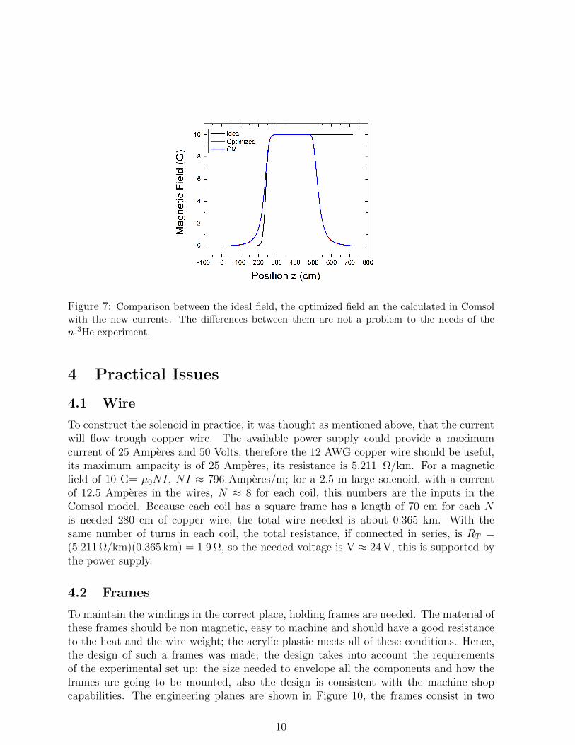
Figure 7: Comparison between the ideal field, the optimized field an the calculated in Comsolwith the new currents. The differences between them are not a problem to the needs of then-3He experiment.

4 Practical Issues

4.1 Wire

To construct the solenoid in practice, it was thought as mentioned above, that the currentwill flow trough copper wire. The available power supply could provide a maximumcurrent of 25 Amperes and 50 Volts, therefore the 12 AWG copper wire should be useful,its maximum ampacity is of 25 Amperes, its resistance is 5.211 Ω/km. For a magneticfield of 10 G= µ0NI, NI ≈ 796 Amperes/m; for a 2.5 m large solenoid, with a currentof 12.5 Amperes in the wires, N ≈ 8 for each coil, this numbers are the inputs in theComsol model. Because each coil has a square frame has a length of 70 cm for each Nis needed 280 cm of copper wire, the total wire needed is about 0.365 km. With thesame number of turns in each coil, the total resistance, if connected in series, is RT =(5.211 Ω/km)(0.365 km) = 1.9 Ω, so the needed voltage is V ≈ 24 V, this is supported bythe power supply.

4.2 Frames

To maintain the windings in the correct place, holding frames are needed. The material ofthese frames should be non magnetic, easy to machine and should have a good resistanceto the heat and the wire weight; the acrylic plastic meets all of these conditions. Hence,the design of such a frames was made; the design takes into account the requirementsof the experimental set up: the size needed to envelope all the components and how theframes are going to be mounted, also the design is consistent with the machine shopcapabilities. The engineering planes are shown in Figure 10, the frames consist in two

10

different pieces which are glued together, in middle there is a channel to put the wire.

11

Figure 8: Several views of the acrylic frame design. The lengths are given in mm. It is intendedto draw how two pieces are constructed to bond together and complete a single frame. a) Thefrontal view is similar for the two pieces; b) the side view of piece 1 shows that this piece has a5 mm step, moreover this piece has a total height of 35 mm and a 25 mm internal height, thewidth is 15 mm; c) the side view of the second piece is similar to the piece 1, but here the 5 mmstep is inverted, therefore the two pieces perfectly match.

12

References

[1] J. D. Bowman et al., A Measurement of the Parity violating Proton Assymmetry inthe Capture of Polarized Cold Neutrons on 3He: A Proposal, Submitted to the SNSFNPB PRAC,(2007).

[2] J. D. Bowman et al., Detector Development for an Experiment to Measure the ParityViolating Proton Asymmetry in the Capture of Polarized Cold Neutrons on 3He,(2008).

[3] R. Alarcon et al., Proposal Update for the n-3He Experiment, (2009).

[4] R. G. Littlejohn, S. Weigert, Adiabatic Motion of a Neutral Spinning Particle in anInhomogeneous Magnetic Field, Physical Review A, VOL. 48, 2, (1993).

[5] S. Balascuta et al., The Implementation of a Super Mirror Polarizer at the SNS Fun-damental Physics Beamline, Nuclear Instruments and Methods in Physics ResearchA, VOL. 671, 137-143 (2012).

[6] J. D. Jackson, Classical Electrodynamics, 3rd Edition, John Wiley & Sons, Inc.,(2001).

[7] C. B. Crawford, Yunchang Shin, A Method for Designing Coils with Arbitrary Fields,Technical Note, (2009).

[8] D. J. Griffiths, Introduction to Electrodynamics, 3rd Edition, Addison Wesley, (1999).

[9] COMSOL, COMSOL Multiphysics User’s Guide, (2012).

[10] COMSOL, Single-Turn and Multi-Turn Coil Domain in 3D Tutorial, (2012).

[11] L. N. Trefethen, D. Bau, Numerical Linear Algebra, Society for Industrial and AppliedMathematics, (1997).