Hollow Heaps

Thomas Dueholm Hansen∗ Haim Kaplan† Robert E. Tarjan‡ Uri Zwick§

Abstract

We introduce the hollow heap, a very simple data structure with the same amortized efficiencyas the classical Fibonacci heap. All heap operations except delete and delete-min take O(1) time,worst case as well as amortized; delete and delete-min take O(log n) amortized time. Hollowheaps are by far the simplest structure to achieve this. Hollow heaps combine two novel ideas:the use of lazy deletion and re-insertion to do decrease-key operations, and the use of a dag(directed acyclic graph) instead of a tree or set of trees to represent a heap. Lazy deletionproduces hollow nodes (nodes without items), giving the data structure its name.

∗Department of Computer Science, Aarhus University, Denmark. Supported by The Danish Council for Indepen-dent Research | Natural Sciences (grant no. 12-126512); and the Sino-Danish Center for the Theory of InteractiveComputation, funded by the Danish National Research Foundation and the National Science Foundation of China(under the grant 61061130540). E-mail: tdh@cs.au.dk.†Blavatnik School of Computer Science, Tel Aviv University, Israel. Research supported by the Israel Science

Foundation grants no. 822-10 and 1841/14, the German-Israeli Foundation for Scientific Research and Development(GIF) grant no. 1161/2011, and the Israeli Centers of Research Excellence (I-CORE) program (Center No. 4/11).E-mail: haimk@post.tau.ac.il.‡Department of Computer Science, Princeton University, Princeton, NJ 08540, USA and Intertrust Technologies,

Sunnyvale, CA 94085, USA.§Blavatnik School of Computer Science, Tel Aviv University, Israel. Research supported by BSF grant no. 2012338

and by The Israeli Centers of Research Excellence (I-CORE) program (Center No. 4/11). E-mail: zwick@tau.ac.il.

1 Introduction

A heap is a data structure consisting of a set of items, each with a key selected from a totallyordered universe. Heaps support the following operations:

make-heap(): Return a new, empty heap.

find-min(h) : Return an item of minimum key in heap h, or null if h is empty.

insert(e, k, h): Return a heap formed from heap h by inserting item e, with key k. Item e must bein no heap.

delete-min(h): Return a heap formed from non-empty heap h by deleting the item returned byfind-min(h).

meld(h1, h2): Return a heap containing all items in item-disjoint heaps h1 and h2.

decrease-key(e, k, h): Given that e is an item in heap h with key greater than k, return a heapformed from h by changing the key of e to k.

delete(e, h) : Return a heap formed by deleting e, assumed to be in h, from h.

The original heap h passed to insert, delete-min, decrease-key, and delete, and the heaps h1 and h2passed to meld, are destroyed by the operations. Heaps do not support search by key; operationsdecrease-key and delete are given the location of item e in heap h. The parameter h can beomitted from decrease-key and delete, but then to make decrease-key operations efficient if thereare intermixed meld operations, a separate disjoint set data structure is needed to keep track of thepartition of items into heaps. (See the discussion in [13].)

Fredman and Tarjan [9] invented the Fibonacci heap, an implementation of heaps that supportsdelete-min and delete on an n-item heap in O(log n) amortized time and each of the other operationsin O(1) amortized time. Applications of Fibonacci heaps include a fast implementation of Dijkstra’sshortest path algorithm [5, 9] and fast algorithms for undirected and directed minimum spanningtrees [7, 10]. Since the invention of Fibonacci heaps, a number of other heap implementationswith the same amortized time bounds have been proposed [1, 2, 4, 8, 11, 12, 14, 17, 19]. Notably,Brodal [1] invented a very complicated heap implementation that achieves the time bounds ofFibonacci heaps in the worst case. Brodal et al. [2] later simplified this data structure, but it is stillsignificantly more complicated than any of the amortized-efficient structures. For further discussionof these and related results, see [11]. We focus here on the amortized efficiency of heaps.

In spite of its many competitors, Fibonacci heaps remain one of the simplest heap implementationsto describe and code, and are taught in numerous undergraduate and graduate data structurescourses. We present Hollow heaps, a data structure that we believe surpasses Fibonacci heaps in itssimplicity. Our data structure has two novelties: it uses lazy deletion to do decrease-key operationsin a simple and natural way, avoiding the cascading cut process used by Fibonacci heaps, and itrepresents a heap by a dag (directed acyclic graph) instead of a tree or a set of trees. The amortizedanalysis of hollow heaps is simple, yet non-trivial. We believe that simplifying fundamental datastructures, while retaining their performance, is an important endeavor.

In a Fibonacci heap, a decrease-key produces a heap-order violation if the new key is less than thatof the parent node. This causes a cut of the violating node and its subtree from its parent. Suchcuts can eventually destroy the “balance” of the data structure. To maintain balance, each such cutmay trigger a cascade of cuts at ancestors of the originally cut node. The cutting process results inloss of information about the outcomes of previous comparisons. It also makes the worst-case time

1

of a decrease-key operation Θ(n) (although modifying the data structure reduces this to Θ(log n);see e.g., [15]). In a hollow heap, the item whose key decreases is merely moved to a new node,preserving the existing structure. Doing such lazy deletions carefully is what makes hollow heapssimple but efficient.

The remainder of our paper consists of eight sections. Section 2 describes hollow heaps at a highlevel. Section 3 analyzes them. Section 4 presents an alternative version of hollow heaps thatuses a tree representation instead of a dag representation. Section 5 describes a rebuilding processthat can be used to improve the time and space efficiency of hollow heaps. Sections 6 and 7 giveimplementation details for the data structures in Sections 2 and 4, respectively. Section 8 exploresthe design space of the data structures in Sections 2 and 4, identifying variants that are efficientand variants that are not. Section 9 contains final remarks.

2 Hollow Heaps

Our data structure extends and refines a well-known generic representation of heaps. The structureis exogenous rather than endogenous [20]: nodes hold items rather than being items. Moving itemsamong nodes precludes the possibility of making the data structure endogenous.

Many previous heap implementations, including Fibonacci heaps, represent a heap by a set of heap-ordered trees: each node holds an item, with each child holding an item having key no less thanthat of the item in its parent. We extend this idea from trees to dags, and to dags whose nodesmay or may not hold items. Since the data structure is an extension of a tree, we extend standardtree terminology to describe it. If (u, v) is a dag arc, we say v is a parent of u and u is a child of v.A node that is not a child of any other node is a root.

We represent a non-empty heap by a dag whose nodes hold the heap items, at most one per node.If e is an item, e.node is the node holding e. We call a node full if it holds an item and hollow ifnot. If u is a full node, u.item is the item u holds. Thus if e is an item, e.node.item = e. A node isfull when created but can later become hollow, by having its item moved to a newly created nodeor deleted. A hollow node remains hollow until it is destroyed. Each node, full or hollow, has akey. The key of a full node is the key of the item it holds. The key of a hollow node is the key ofthe item it once held, just before that item was moved to another node or deleted. A full node isa child of at most one other node; a hollow node is a child of at most two other nodes.

The dag is topologically ordered by key: if u is a child of v, then u.key ≥ v.key. Henceforth wecall this heap order. Except in the middle of a delete operation, the dag has one full root and nohollow roots. Heap order guarantees that the root holds an item of minimum key. We access thedag via its root. We call the item in the root the root item.

We do the heap operations with the help of the link primitive. Given two full roots v and w,link(v, w) compares the keys of v and w and makes the root of larger key a child of the other; ifthe keys are equal, it makes v a child of w. The new child is the loser of the link, its new parentis the winner. Linking eliminates one full root, preserves heap order, and gives the loser a parent,its first parent.

To make a heap, return an empty dag. To do find-min, return the item in the root. To meld twoheaps, if one is empty return the other; if both are non-empty, link the roots of their dags andreturn the winner. To insert an item into a heap, create a new node, store the item in it (makingthe node full), and meld the resulting one-node heap with the existing heap.

We do decrease-key and delete operations using lazy deletion. To decrease the key of item e inheap h to k, let u = e.node. If u = h (u is the root of the dag), merely set u.key = k. Otherwise(u is a child), proceed as follows. Create a new node v; move e from u to v, making u hollow; set

2

v.key = k; do link(h, v); and, if v is the loser of this link, make u a child of v. If u becomes a childof v, then v is the second parent of u, in contrast to its first parent, previously acquired via a linkwith a full node. A node only becomes hollow once, so it acquires a second parent at most once.

To do a delete-min, do a find-min followed by a deletion of the returned item. To delete an item e,remove e from the node holding it, say u, making u hollow. A node u made hollow in this waynever acquires a second parent. If u is not the root of the dag, the deletion is complete. Otherwise,repeatedly destroy hollow roots and link full roots until there are no hollow roots and at most onefull root.

Theorem 2.1 The hollow heap operations perform the heap operations correctly and maintain theinvariants that the graph representing a heap is a heap-ordered dag; each full node has at most oneparent; each hollow node has at most two parents; and, except in the middle of a delete operation,the dag representing a heap has no hollow roots and at most one full root.

Proof: Immediate. 2

The only flexibility in this implementation is the choice of which links to do in deletions of rootitems. To keep the number of links small, we give each node u a non-negative integer rank u.rank.We use ranks in a special kind of link called a ranked link. A ranked link of two roots is allowedonly if they have the same rank; it links them and increases the rank of the winner (the remainingroot) by 1. In contrast to a ranked link, an unranked link links any two roots and changes noranks. We call a child ranked or unranked if it most recently acquired a first parent via a rankedor unranked link, respectively.

When linking two roots of equal rank, we can do either a ranked or an unranked link. We doranked links only when needed to guarantee efficiency. Specifically, links in meld and decrease-keyare unranked. Each delete-min operation destroys hollow roots and does ranked links until noneare possible (there are no hollow roots and all full roots have different ranks); then it does unrankedlinks until there is at most one root.

The last design choice is the initial node ranks. We give a node created by an insert a rankof 0. In a decrease-key that moves an item from a node u to a new node v, we give v a rank ofmax0, u.rank− 2. The latter choice is what makes hollow heaps efficient.

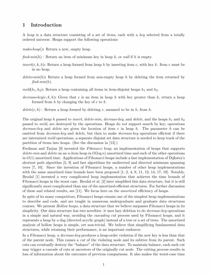
Figure 1 shows a sequence of operations on a hollow heap.

We conclude this section by mentioning some benefits of using hollow nodes and a dag representa-tion. Hollow nodes allow us to treat decrease-key as a special kind of insertion, allowing us to avoidcutting subtrees as in Fibonacci heaps. As a consequence, decrease-key takes O(1) time worst case:there are no cascading cuts as in [9], no cascading rank changes as in [11, 15], and no restructuringsteps to eliminate heap-order violations as in [2, 6, 14]. The dag representation explicitly maintainsall key comparisons between undeleted items, allowing us to avoid restructuring altogether: linksare cut only when hollow roots are destroyed.

3 Analysis

The most mysterious detail of hollow heaps is the way ranks are updated in decrease-key operations.Our analysis reveals the reason for this choice. We need to show that the rank of a heap node is atmost logarithmic in the number of nodes in the dag representing the heap, and that the amortizednumber of ranked children per node is also at most logarithmic.

3

0

4 13 12 6 3 10 8 5

9 11

14

33

4 5 102 1

6 13 8 9 111

12 14

1

33

4 5 102 1

6 13 8 9 111

12 14

(a) (b) (c)

1

7 21

33

4 5 102 1

6 13 8 9 111

12 14

7

21

33

4 5 102 1

6 13 8 9 111

12 14

43

7 6 132 1

9 10 8 121

11

14

(d) (e) (f)

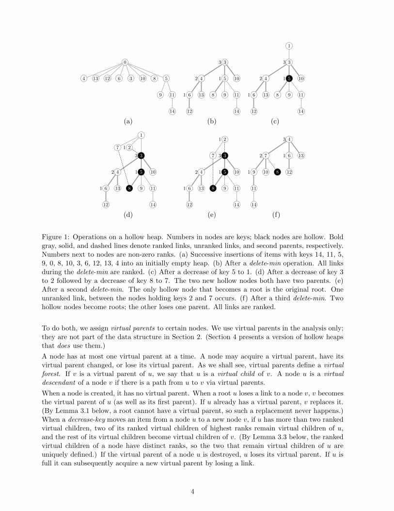
Figure 1: Operations on a hollow heap. Numbers in nodes are keys; black nodes are hollow. Boldgray, solid, and dashed lines denote ranked links, unranked links, and second parents, respectively.Numbers next to nodes are non-zero ranks. (a) Successive insertions of items with keys 14, 11, 5,9, 0, 8, 10, 3, 6, 12, 13, 4 into an initially empty heap. (b) After a delete-min operation. All linksduring the delete-min are ranked. (c) After a decrease of key 5 to 1. (d) After a decrease of key 3to 2 followed by a decrease of key 8 to 7. The two new hollow nodes both have two parents. (e)After a second delete-min. The only hollow node that becomes a root is the original root. Oneunranked link, between the nodes holding keys 2 and 7 occurs. (f) After a third delete-min. Twohollow nodes become roots; the other loses one parent. All links are ranked.

To do both, we assign virtual parents to certain nodes. We use virtual parents in the analysis only;they are not part of the data structure in Section 2. (Section 4 presents a version of hollow heapsthat does use them.)

A node has at most one virtual parent at a time. A node may acquire a virtual parent, have itsvirtual parent changed, or lose its virtual parent. As we shall see, virtual parents define a virtualforest. If v is a virtual parent of u, we say that u is a virtual child of v. A node u is a virtualdescendant of a node v if there is a path from u to v via virtual parents.

When a node is created, it has no virtual parent. When a root u loses a link to a node v, v becomesthe virtual parent of u (as well as its first parent). If u already has a virtual parent, v replaces it.(By Lemma 3.1 below, a root cannot have a virtual parent, so such a replacement never happens.)When a decrease-key moves an item from a node u to a new node v, if u has more than two rankedvirtual children, two of its ranked virtual children of highest ranks remain virtual children of u,and the rest of its virtual children become virtual children of v. (By Lemma 3.3 below, the rankedvirtual children of a node have distinct ranks, so the two that remain virtual children of u areuniquely defined.) If the virtual parent of a node u is destroyed, u loses its virtual parent. If u isfull it can subsequently acquire a new virtual parent by losing a link.

4

Lemma 3.1 If w is a virtual child of u, there is a path in the dag from w to u.

Proof: We prove the lemma for a given node w by induction on time. When w is created it hasno virtual parent. It may acquire a virtual parent only by losing a link to a node u, which thenbecomes both its parent and its virtual parent, so the lemma holds after the link. Suppose that uis currently the virtual parent of w. By the induction hypothesis, there is a path from w to u inthe dag, so w is not a root and cannot participate in link operations. The virtual parent of wcan change only as a result of a decrease-key operation on the item e = u.item. If u 6= h, such adecrease-key operation creates a new node v, moves e to v, and then links v and h. The operationmay also make v the new virtual parent of w. If v wins the link, it becomes the unique root andthere is clearly a path from w to v in the dag. If v loses the link, the arc (u, v) is added to the dag,making v the second parent of u. Since there was a path in the dag from w to u, there is now also apath from w to v. Finally, note that dag arcs are only destroyed when hollow roots are destroyed.Thus a path from w to its virtual parent u in the dag, present when u becomes the virtual parentof w, cannot be destroyed unless u is destroyed, in which case w loses its virtual parent, so thelemma holds vacuously. 2

The arc (u, v) added to the dag by decrease-key represents the inequality u.key > v.key. If this arcis not redundant and decrease-key fails to add it, our analysis breaks down. Indeed, the resultingalgorithm does not have the desired efficiency, as we show in Section 8. Adding the arc only whenv loses the link to h is an optimization: if v wins the link, the dag has a path from u to v withoutit.

Corollary 3.2 Virtual parents define a forest. If w is a root of the dag, it has no virtual parent.If w is a virtual child of u, then w stops being a virtual child of u only when u is destroyed or whena decrease-key operation is applied to the item residing in u.

Lemma 3.3 Let u be a node of rank r. If u is full, or u is a node made hollow by a delete, u hasexactly one ranked virtual child of each rank from 0 to r−1 inclusive, and none of rank r or greater.If u was made hollow by a decrease-key and r > 1, u has exactly two ranked virtual children, ofranks r− 1 and r− 2. If u was made hollow by a decrease-key and r = 1, u has exactly one rankedvirtual child, of rank 0. If u was made hollow by a decrease-key and r = 0, u has no ranked virtualchildren.

Proof: The proof is by induction on the number of operations. The lemma is immediate for nodescreated by insertions. Both ranked and unranked links preserve the truth of the lemma, as doesthe removal of an item from a node by a delete. By Corollary 3.2, a node loses virtual childrenonly as a result of a decrease-key operation. Suppose the lemma is true before a decrease-key onthe item in a node u of rank r. By the induction hypothesis, u has exactly one ranked virtual childof rank i for 0 ≤ i < r, and none of rank r or greater. If the decrease-key makes u hollow, thenew node v created by the decrease-key has rank max0, u.rank− 2, and v acquires all the virtualchildren of u except the two ranked virtual children of ranks r − 1 and r − 2 if r > 1, or the oneranked virtual child of rank 0 if r = 1. Thus the lemma holds after the decrease-key. 2

Recall the definition of the Fibonacci numbers: F0 = 0, F1 = 1, Fi = Fi−1 + Fi−2 for i ≥ 2. Thesenumbers satisfy Fi+2 ≥ φi, where φ = (1 +

√5)/2 is the golden ratio [16].

Corollary 3.4 A node of rank r has at least Fr+3 − 1 virtual descendants.

5

Proof: The proof is by induction on r using Lemma 3.3. The corollary is immediate for r = 0and r = 1. If r > 1, the virtual descendants of a node u of rank r include itself and all virtualdescendants of its virtual children v and w of ranks r − 1 and r − 2, which it has by Lemma 3.3.By Corollary 3.2, virtual parents define a forest, so the sets of virtual descendants of v and w aredisjoint. By the induction hypothesis, u has at least 1 + Fr+2 − 1 + Fr+1 − 1 = Fr+3 − 1 virtualdescendants. 2

Theorem 3.5 The maximum rank of a node in a hollow heap of N nodes is at most logφN .

Proof: Immediate from Corollary 3.4 since Fr+3 − 1 ≥ Fr+2 ≥ φr for r ≥ 0. 2

To complete our analysis, we need to bound the time of an arbitrary sequence of heap operationsthat starts with no heaps. It is straightforward to implement the operations so that the worst-casetime per operation other than delete-min and delete is O(1), and that of a delete on a heap of Nnodes is O(1) plus O(1) per hollow node that loses a parent plus O(1) per link plus O(logN). InSection 6 we give an implementation that satisfies these bounds and is space-efficient. We shallshow that the amortized time for a delete on a heap of N nodes is O(logN) by charging the parentlosses of hollow nodes and some of the links to other operations, O(1) per operation.

Suppose a hollow node u loses a parent in a delete. This either makes u a root, in which case u isdestroyed by the same delete, or it reduces the number of parents of u from two to one. We chargethe former case to the insert or decrease-key that created u, and the latter case to the decrease-keythat gave u its second parent. Since an insert or decrease-key can create at most one node, anda decrease-key can give at most one node a second parent, the total charge, and hence the totalnumber of parent losses of hollow nodes, is at most 1 per insert and 2 per decrease-key.

A delete does unranked links only once there is at most one root per rank. Thus the numberof unranked links is at most the maximum node rank, which is at most logφN by Theorem 3.5.To bound the number of ranked links, we use a potential argument. We give each root and eachunranked child a potential of 1. We give a ranked child a potential of 0 if it has a full virtualparent, 1 otherwise (its virtual parent is hollow or has been deleted). We define the potential of aset of dags to be the sum of the potentials of their nodes. With this definition the initial potentialis 0 (there are no nodes), and the potential is always non-negative. Each ranked link reduces thepotential by 1: a root becomes a ranked child of a full node. It follows that the total number ofranked links over a sequence of operations is at most the sum of the increases in potential producedby the operations.

An unranked link does not change the potential: a root becomes an unranked child. An insertincreases the potential by 1: it creates a new root (+1) and does an unranked link (+0). Adecrease-key increases the potential by at most 3: it creates a new root (+1), it creates a hollownode that has at most two ranked virtual children by Lemma 3.3 (+2), and it does an unrankedlink (+0). Removing the item in a node u during a delete increases the potential by u.rank, also byLemma 3.3: each ranked virtual child of u gains 1 in potential. By Theorem 3.5, u.rank = O(logN).We conclude that the total number of ranked links is at most 1 per insert plus 3 per decrease-keyplus O(logN) per delete on a heap with N nodes. Combining our bounds gives the followingtheorem:

Theorem 3.6 The amortized time per hollow heap operation is O(1) for each operation other thana delete, and O(logN) per delete on a heap of N nodes.

6

4 Eager Hollow Heaps

It is natural to ask whether there is a way to represent a hollow heap by a tree instead of a dag.The answer is yes: we maintain the structure defined by the virtual parents instead of that definedby the parents. We call this the eager version of hollow heaps: it moves children among nodes,which the lazy version in Section 2 does not do. As a result it can do different links than the lazyversion, but it has the same amortized efficiency.

To obtain eager hollow heaps, we modify decrease-key as follows: When a new node v is created tohold the item previously in a node u, if u.rank > 2, make v the parent of all but the two rankedchildren of u of highest ranks; optionally, make v the parent of some or all of the unranked childrenof u. Do not make u a child of v.

In an eager hollow heap, each node has at most one parent. Thus each heap is represented by atree, accessed via its root. The analysis of eager hollow heaps differs from that of lazy hollow heapsonly in using parents instead of virtual parents. Only the parents of ranked children matter in theanalysis.

The proofs of the following results are essentially identical to the proofs of the results in Section 2,with the word “virtual” deleted.

Lemma 4.1 Let u be a node of rank r in an eager hollow heap. If u is full, or u is a node madehollow by a delete, u has exactly one ranked child of each rank from 0 to r− 1 inclusive, and noneof rank r or greater. If u was made hollow by a decrease-key and r > 1, u has exactly two rankedchildren, of ranks r− 1 and r− 2. If u was made hollow by a decrease-key and r = 1, u has exactlyone ranked child, of rank 0. If u was made hollow by a decrease-key and r = 0, u has no rankedchildren.

Corollary 4.2 A node of rank r in an eager hollow heap has at least Fr+3 − 1 descendants.

Theorem 4.3 The maximum rank of a node in an eager hollow heap of N nodes is at most logφN .

Theorem 4.4 The amortized time per eager hollow heap operation is O(1) for each operation otherthan a delete, and O(logN) per delete on a heap of N nodes.

An alternative way to think about eager hollow heaps is as a variant of Fibonacci heaps. In aFibonacci heap, the cascading cuts that occur during a decrease-key prune the tree in a way thatguarantees that ranks remain logarithmic in subtree sizes. Eager hollow heaps guarantee logarithmicranks by leaving (at least) two children and a hollow node behind at the site of the cut. This avoidsthe need for cascading cuts or rank changes, and makes the decrease-key operation O(1) time inthe worst case.

5 Rebuilding

The number of nodes N in a heap is at most the number of items n plus the number of decrease-keyoperations on items that were ever in the heap or in heaps melded into it. If the number ofdecrease-key operations is polynomial in the number of insertions, logN = O(log n), so the amor-tized time per delete is O(log n), the same as for Fibonacci heaps. In applications in which thestorage required for the problem input is at least linear in the number of heap operations, the extraspace needed for hollow nodes is linear in the problem size. Both of these conditions hold for theheaps used in many graph algorithms, including Dijkstra’s shortest path algorithm [5, 9], various

7

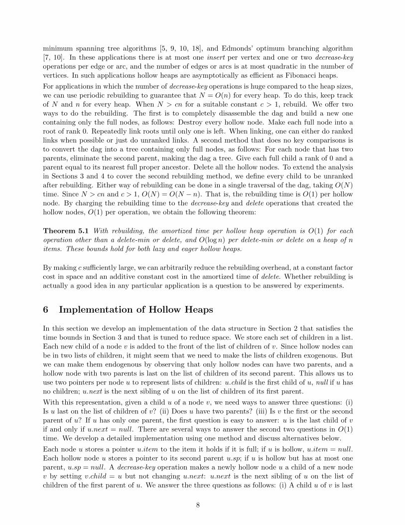
minimum spanning tree algorithms [5, 9, 10, 18], and Edmonds’ optimum branching algorithm[7, 10]. In these applications there is at most one insert per vertex and one or two decrease-keyoperations per edge or arc, and the number of edges or arcs is at most quadratic in the number ofvertices. In such applications hollow heaps are asymptotically as efficient as Fibonacci heaps.

For applications in which the number of decrease-key operations is huge compared to the heap sizes,we can use periodic rebuilding to guarantee that N = O(n) for every heap. To do this, keep trackof N and n for every heap. When N > cn for a suitable constant c > 1, rebuild. We offer twoways to do the rebuilding. The first is to completely disassemble the dag and build a new onecontaining only the full nodes, as follows: Destroy every hollow node. Make each full node into aroot of rank 0. Repeatedly link roots until only one is left. When linking, one can either do rankedlinks when possible or just do unranked links. A second method that does no key comparisons isto convert the dag into a tree containing only full nodes, as follows: For each node that has twoparents, eliminate the second parent, making the dag a tree. Give each full child a rank of 0 and aparent equal to its nearest full proper ancestor. Delete all the hollow nodes. To extend the analysisin Sections 3 and 4 to cover the second rebuilding method, we define every child to be unrankedafter rebuilding. Either way of rebuilding can be done in a single traversal of the dag, taking O(N)time. Since N > cn and c > 1, O(N) = O(N − n). That is, the rebuilding time is O(1) per hollownode. By charging the rebuilding time to the decrease-key and delete operations that created thehollow nodes, O(1) per operation, we obtain the following theorem:

Theorem 5.1 With rebuilding, the amortized time per hollow heap operation is O(1) for eachoperation other than a delete-min or delete, and O(log n) per delete-min or delete on a heap of nitems. These bounds hold for both lazy and eager hollow heaps.

By making c sufficiently large, we can arbitrarily reduce the rebuilding overhead, at a constant factorcost in space and an additive constant cost in the amortized time of delete. Whether rebuilding isactually a good idea in any particular application is a question to be answered by experiments.

6 Implementation of Hollow Heaps

In this section we develop an implementation of the data structure in Section 2 that satisfies thetime bounds in Section 3 and that is tuned to reduce space. We store each set of children in a list.Each new child of a node v is added to the front of the list of children of v. Since hollow nodes canbe in two lists of children, it might seem that we need to make the lists of children exogenous. Butwe can make them endogenous by observing that only hollow nodes can have two parents, and ahollow node with two parents is last on the list of children of its second parent. This allows us touse two pointers per node u to represent lists of children: u.child is the first child of u, null if u hasno children; u.next is the next sibling of u on the list of children of its first parent.

With this representation, given a child u of a node v, we need ways to answer three questions: (i)Is u last on the list of children of v? (ii) Does u have two parents? (iii) Is v the first or the secondparent of u? If u has only one parent, the first question is easy to answer: u is the last child of vif and only if u.next = null. There are several ways to answer the second two questions in O(1)time. We develop a detailed implementation using one method and discuss alternatives below.

Each node u stores a pointer u.item to the item it holds if it is full; if u is hollow, u.item = null.Each hollow node u stores a pointer to its second parent u.sp; if u is hollow but has at most oneparent, u.sp = null. A decrease-key operation makes a newly hollow node u a child of a new nodev by setting v.child = u but not changing u.next: u.next is the next sibling of u on the list ofchildren of the first parent of u. We answer the three questions as follows: (i) A child u of v is last

8

on the list of children of v if and only if u.next = null (u is last on any list of children containingit) or u.sp = v (u is hollow with two parents and v is its second parent); (ii) u has two parents ifand only if u.sp 6= null; (iii) v is the second parent of u if and only if u.sp = v.

Each node u also stores its key and rank, and each item e stores the node e.node holding it. Thetotal space needed is four pointers, a key, and a rank per node, and one pointer per item. Ranksare small integers, each requiring lg lgN +O(1) bits of space.

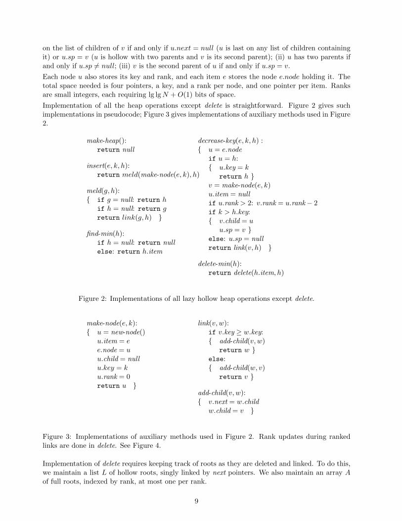
Implementation of all the heap operations except delete is straightforward. Figure 2 gives suchimplementations in pseudocode; Figure 3 gives implementations of auxiliary methods used in Figure2.

make-heap():return null

insert(e, k, h):return meld(make-node(e, k), h)

meld(g, h): if g = null: return h

if h = null: return greturn link(g, h)

find-min(h):if h = null: return nullelse: return h.item

decrease-key(e, k, h) : u = e.node

if u = h: u.key = k

return h v = make-node(e, k)u.item = nullif u.rank > 2: v.rank = u.rank− 2if k > h.key: v.child = u

u.sp = v else: u.sp = nullreturn link(v, h)

delete-min(h):return delete(h.item, h)

Figure 2: Implementations of all lazy hollow heap operations except delete.

make-node(e, k): u = new-node()

u.item = ee.node = uu.child = nullu.key = ku.rank = 0return u

link(v, w):if v.key ≥ w.key: add-child(v, w)

return w else: add-child(w, v)

return v

add-child(v, w): v.next = w.child

w.child = v

Figure 3: Implementations of auxiliary methods used in Figure 2. Rank updates during rankedlinks are done in delete. See Figure 4.

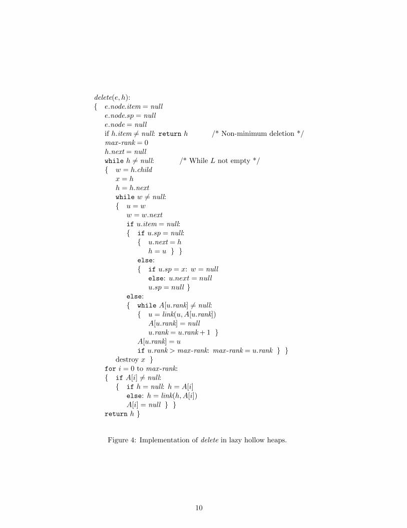
Implementation of delete requires keeping track of roots as they are deleted and linked. To do this,we maintain a list L of hollow roots, singly linked by next pointers. We also maintain an array Aof full roots, indexed by rank, at most one per rank.

9

delete(e, h): e.node.item = null

e.node.sp = nulle.node = nullif h.item 6= null: return h /* Non-minimum deletion */max -rank = 0h.next = nullwhile h 6= null: /* While L not empty */ w = h.child

x = hh = h.nextwhile w 6= null: u = w

w = w.nextif u.item = null: if u.sp = null: u.next = h

h = u else: if u.sp = x: w = null

else: u.next = nullu.sp = null

else: while A[u.rank] 6= null: u = link(u,A[u.rank])

A[u.rank] = nullu.rank = u.rank + 1

A[u.rank] = uif u.rank > max -rank: max -rank = u.rank

destroy x for i = 0 to max -rank: if A[i] 6= null: if h = null: h = A[i]

else: h = link(h,A[i])A[i] = null

return h

Figure 4: Implementation of delete in lazy hollow heaps.

10

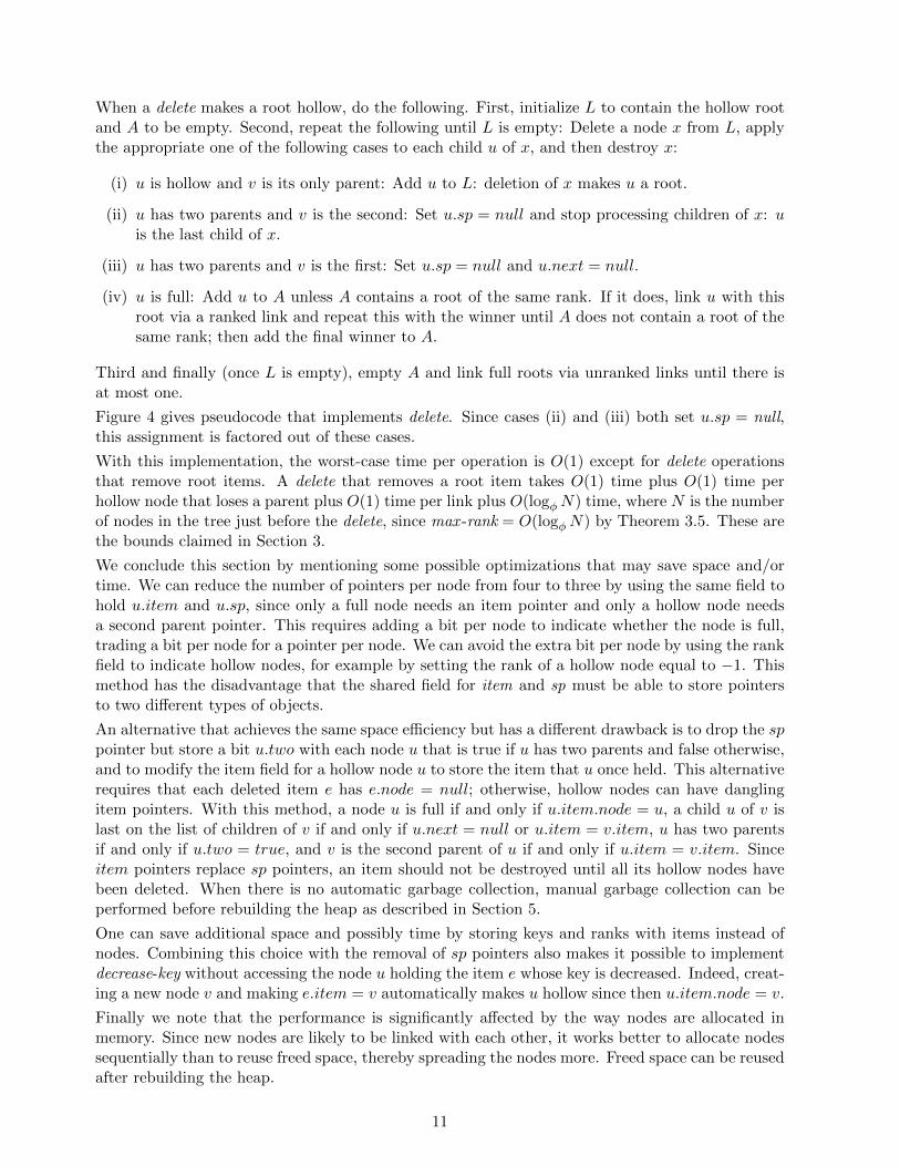
When a delete makes a root hollow, do the following. First, initialize L to contain the hollow rootand A to be empty. Second, repeat the following until L is empty: Delete a node x from L, applythe appropriate one of the following cases to each child u of x, and then destroy x:

(i) u is hollow and v is its only parent: Add u to L: deletion of x makes u a root.

(ii) u has two parents and v is the second: Set u.sp = null and stop processing children of x: uis the last child of x.

(iii) u has two parents and v is the first: Set u.sp = null and u.next = null.

(iv) u is full: Add u to A unless A contains a root of the same rank. If it does, link u with thisroot via a ranked link and repeat this with the winner until A does not contain a root of thesame rank; then add the final winner to A.

Third and finally (once L is empty), empty A and link full roots via unranked links until there isat most one.

Figure 4 gives pseudocode that implements delete. Since cases (ii) and (iii) both set u.sp = null,this assignment is factored out of these cases.

With this implementation, the worst-case time per operation is O(1) except for delete operationsthat remove root items. A delete that removes a root item takes O(1) time plus O(1) time perhollow node that loses a parent plus O(1) time per link plus O(logφN) time, where N is the numberof nodes in the tree just before the delete, since max -rank = O(logφN) by Theorem 3.5. These arethe bounds claimed in Section 3.

We conclude this section by mentioning some possible optimizations that may save space and/ortime. We can reduce the number of pointers per node from four to three by using the same field tohold u.item and u.sp, since only a full node needs an item pointer and only a hollow node needsa second parent pointer. This requires adding a bit per node to indicate whether the node is full,trading a bit per node for a pointer per node. We can avoid the extra bit per node by using the rankfield to indicate hollow nodes, for example by setting the rank of a hollow node equal to −1. Thismethod has the disadvantage that the shared field for item and sp must be able to store pointersto two different types of objects.

An alternative that achieves the same space efficiency but has a different drawback is to drop the sppointer but store a bit u.two with each node u that is true if u has two parents and false otherwise,and to modify the item field for a hollow node u to store the item that u once held. This alternativerequires that each deleted item e has e.node = null; otherwise, hollow nodes can have danglingitem pointers. With this method, a node u is full if and only if u.item.node = u, a child u of v islast on the list of children of v if and only if u.next = null or u.item = v.item, u has two parentsif and only if u.two = true, and v is the second parent of u if and only if u.item = v.item. Sinceitem pointers replace sp pointers, an item should not be destroyed until all its hollow nodes havebeen deleted. When there is no automatic garbage collection, manual garbage collection can beperformed before rebuilding the heap as described in Section 5.

One can save additional space and possibly time by storing keys and ranks with items instead ofnodes. Combining this choice with the removal of sp pointers also makes it possible to implementdecrease-key without accessing the node u holding the item e whose key is decreased. Indeed, creat-ing a new node v and making e.item = v automatically makes u hollow since then u.item.node = v.

Finally we note that the performance is significantly affected by the way nodes are allocated inmemory. Since new nodes are likely to be linked with each other, it works better to allocate nodessequentially than to reuse freed space, thereby spreading the nodes more. Freed space can be reusedafter rebuilding the heap.

11

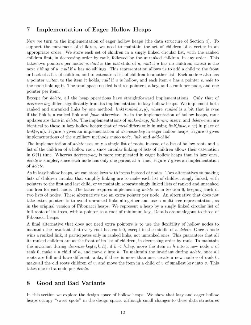
7 Implementation of Eager Hollow Heaps

Now we turn to the implementation of eager hollow heaps (the data structure of Section 4). Tosupport the movement of children, we need to maintain the set of children of a vertex in anappropriate order. We store each set of children in a singly linked circular list, with the rankedchildren first, in decreasing order by rank, followed by the unranked children, in any order. Thistakes two pointers per node: u.child is the last child of u, null if u has no children; u.next is thenext sibling of u, null if u has no siblings. This representation allows us to add a child to the frontor back of a list of children, and to catenate a list of children to another list. Each node u also hasa pointer u.item to the item it holds, null if u is hollow, and each item e has a pointer e.node tothe node holding it. The total space needed is three pointers, a key, and a rank per node, and onepointer per item.

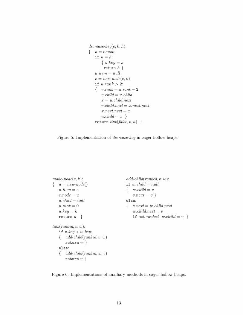
Except for delete, all the heap operations have straightforward implementations. Only that ofdecrease-key differs significantly from its implementation in lazy hollow heaps. We implement bothranked and unranked links by one method, link(ranked, x, y), where ranked is a bit that is trueif the link is a ranked link and false otherwise. As in the implementation of hollow heaps, rankupdates are done in delete. The implementations of make-heap, find-min, insert, and delete-min areidentical to those in lazy hollow heaps; that of meld differs only in using link(false, v, w) in place oflink(v, w). Figure 5 gives an implementation of decrease-key in eager hollow heaps; Figure 6 givesimplementations of the auxiliary methods make-node, link, and add-child.

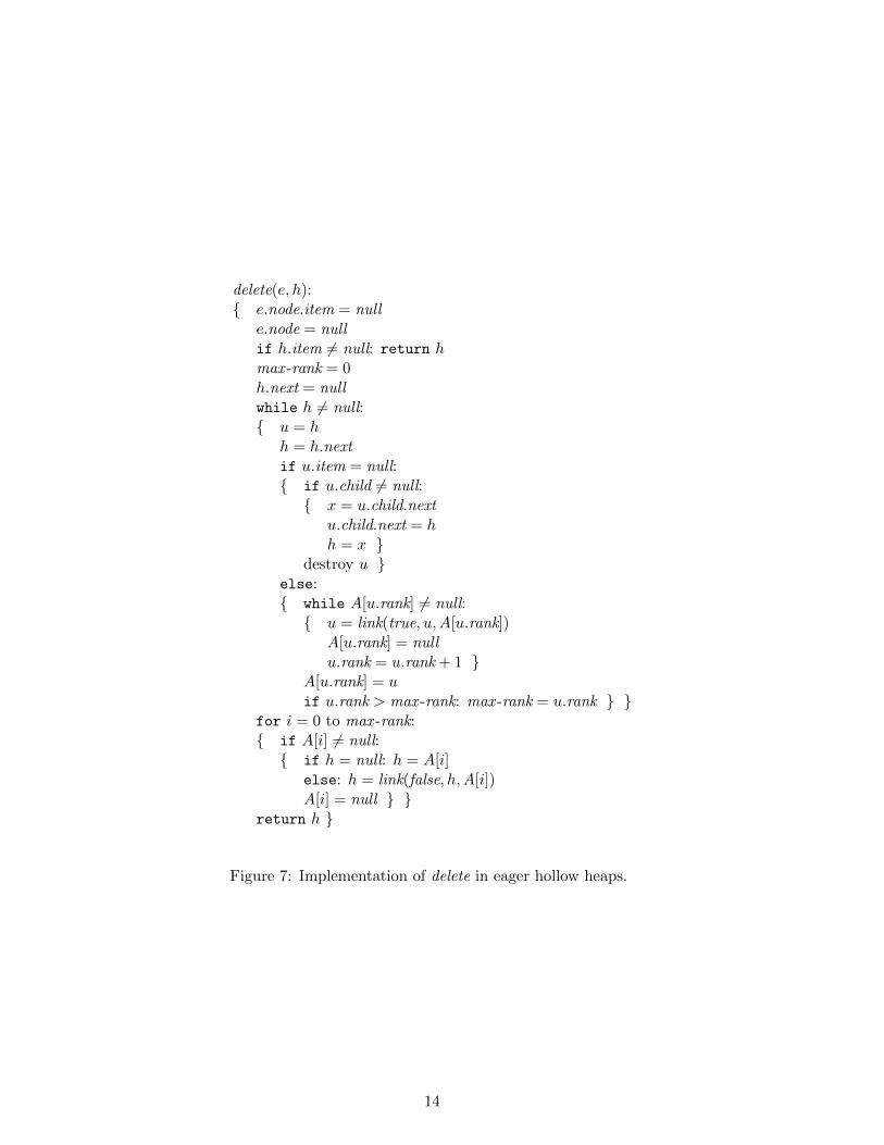
The implementation of delete uses only a single list of roots, instead of a list of hollow roots and alist of the children of a hollow root, since circular linking of lists of children allows their catenationin O(1) time. Whereas decrease-key is more complicated in eager hollow heaps than in lazy ones,delete is simpler, since each node has only one parent at a time. Figure 7 gives an implementationof delete.

As in lazy hollow heaps, we can store keys with items instead of nodes. Two alternatives to makinglists of children circular that simplify linking are to make each list of children singly linked, withpointers to the first and last child, or to maintain separate singly linked lists of ranked and unrankedchildren for each node. The latter requires implementing delete as in Section 6, keeping track oftwo lists of nodes. These alternatives use an extra pointer per node. An alternative that does nottake extra pointers is to avoid unranked links altogether and use a multi-tree representation, asin the original version of Fibonacci heaps. We represent a heap by a singly linked circular list offull roots of its trees, with a pointer to a root of minimum key. Details are analogous to those ofFibonacci heaps.

A final alternative that does not need extra pointers is to use the flexibility of hollow nodes tomaintain the invariant that every root has rank 0, except in the middle of a delete. Once a nodewins a ranked link, it participates only in ranked links, not unranked ones. This guarantees that allits ranked children are at the front of its list of children, in decreasing order by rank. To maintainthe invariant during decrease-key(e, k, h), if k < h.key, move the item in h into a new node v ofrank 0, make v a child of h, and move e into h. To maintain the invariant during delete, once allroots are full and have different ranks, if there is more than one, create a new node v of rank 0,make all the old roots children of v, and move the item in a child of v of smallest key into v. Thistakes one extra node per delete.

8 Good and Bad Variants

In this section we explore the design space of hollow heaps. We show that lazy and eager hollowheaps occupy “sweet spots” in the design space: although small changes to these data structures

12

decrease-key(e, k, h): u = e.node

if u = h: u.key = k

return h u.item = nullv = new-node(e, k)if u.rank > 2: v.rank = u.rank− 2

v.child = u.childx = u.child.nextv.child.next = x.next.nextx.next.next = xu.child = x

return link(false, v, h)

Figure 5: Implementation of decrease-key in eager hollow heaps.

make-node(e, k): u = new-node()

u.item = ee.node = uu.child = nullu.rank = 0u.key = kreturn u

link(ranked, v, w):if v.key > w.key: add-child(ranked, v, w)

return w else: add-child(ranked, w, v)

return v

add-child(ranked, v, w):if w.child = null: w.child = v

v.next = v else: v.next = w.child.next

w.child.next = vif not ranked: w.child = v

Figure 6: Implementations of auxiliary methods in eager hollow heaps.

13

delete(e, h): e.node.item = null

e.node = nullif h.item 6= null: return hmax -rank = 0h.next = nullwhile h 6= null: u = h

h = h.nextif u.item = null: if u.child 6= null: x = u.child.next

u.child.next = hh = x

destroy u else: while A[u.rank] 6= null: u = link(true, u, A[u.rank])

A[u.rank] = nullu.rank = u.rank + 1

A[u.rank] = uif u.rank > max -rank: max -rank = u.rank

for i = 0 to max -rank: if A[i] 6= null: if h = null: h = A[i]

else: h = link(false, h, A[i])A[i] = null

return h

Figure 7: Implementation of delete in eager hollow heaps.

14

preserve their efficiency, larger changes destroy it. We consider three classes of data structures:lazy-k, eager -k, and naıve-k. Here k is an integer parameter specifying the rank of the new node vin a decrease-key operation. In specifying k we use r to denote the rank of the node u made hollowby the decrease-key operation. Data structure lazy-k is the data structure of Section 2, except thatit sets the rank of v in decrease-key to be maxk, 0. Thus lazy-(r−2) is exactly the data structureof Section 2. Data structure eager -k is the data structure of Section 4, except that it sets the rankof v in decrease-key to be maxk, 0, and, if r > k, it moves to v all but the r − k highest-rankedranked children of u, as well as the unranked children of u. Thus eager -(r − 2) is exactly the datastructure of Section 4. Finally, naıve-k is the data structure of Section 2, except that it sets therank of v in decrease-key to be maxk, 0 and it never assigns second parents: when a hollow node ubecomes a root, u is deleted and all its children become roots. We consider two regimes for k: large,in which k = r − j for some fixed non-negative integer j; and small, in which k = r − f(r), wheref(r) is a positive non-decreasing integer function that tends to infinity as r tends to infinity.

We begin with a positive result: for any fixed integer j ≥ 2, both lazy-(r − j) and eager -(r − j)have the efficiency of Fibonacci heaps. It is straightforward to prove this by adapting the analysisin Sections 3 and 4. As j increases, the rank bound (Theorems 3.5 and 4.3) decreases by a constantfactor, approaching lgN or lg n, respectively, as j grows, where lg is the base-2 logarithm. Thetrade-off is that the amortized time bound for decrease-key is O(j + 1), increasing linearly with j.

All other variants are inefficient. Specifically, if the amortized time per delete-min is O(logm),where m is the total number of operations, and the amortized time per make-heap and insert isO(1), then the amortized time per decrease-key is ω(1). We demonstrate this by constructingcostly sequences of operations for each variant. We content ourselves merely with showing thatthe amortized time per decrease-key is ω(1); for at least some variants, there are asymptoticallyworse sequences than ours. Our results are summarized in the following theorem. The individualconstructions appear in Sections 8.1, 8.2, and 8.3.

Theorem 8.1 Variants lazy-(r − j) and eager-(r − j) are efficient for any choice of j > 1 fixedindependent of r. All other variants, namely naıve-k for all k, eager-r, lazy-r, eager-(r − 1),lazy-(r − 1), and eager-k and lazy-k for k in the small regime are inefficient.

8.1 Eager-k for k in the small regime and naıve-k for all k

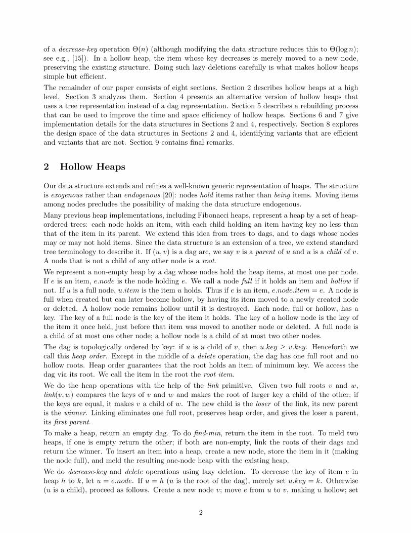
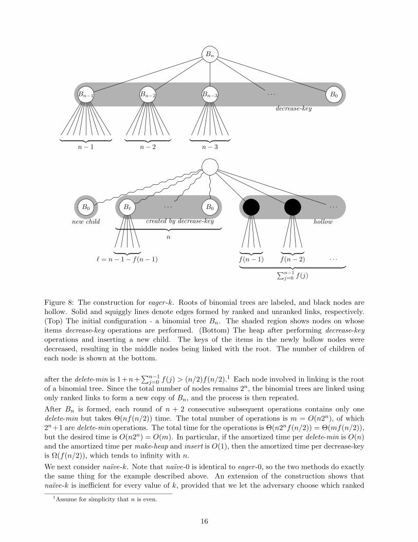
We first consider eager -k for k in the small regime, i.e., k = r − f(r) where f is a positive non-decreasing function that tends to infinity. We obtain an expensive sequence of operations as follows.We define the binomial tree Bn [3, 21] inductively: B0 is a one-node tree; Bn+1 is formed by linkingthe roots of two copies of Bn. Tree Bn consists of a root whose children are the roots of copies ofB0, B1, . . . , Bn−1 [3, 21]. For any n, build a Bn by beginning with an empty tree and doing 2n + 1insertions of items in increasing order by key followed by one delete-min. After the insertions, thetree will consist of a root with 2n children of rank 0. In the delete-min, all the links will be ranked,and they will produce a copy of Bn in which each node that is the root of a copy of Bj has rank j.The tree Bn is shown at the top of Figure 8.

Now repeat the following n+ 2 operations 2n times: do n decrease-key operations on the items inthe children of the root of Bn, making the new keys greater than that of the key of the item in theroot. This makes the n previous children of the root hollow, and gives the root n new children.Insert a new item whose key is greater than that of the item in the root. Finally, do a delete-min.The delete-min deletes the root and its n hollow children, leaving the children of the hollow nodesto be linked. Since a hollow node of rank r has f(r) children, the total number of nodes linked

15

new child

︸ ︷︷ ︸︸ ︷︷ ︸n− 1

︸ ︷︷ ︸n− 2

︸ ︷︷ ︸n− 3

decrease-key

Bn

Bn−1 Bn−2 Bn−3 · · · B0

new child

︸ ︷︷ ︸ ︸ ︷︷ ︸f(n− 1)

︸ ︷︷ ︸f(n− 2) · · ·︸ ︷︷ ︸∑n−1j=0 f(j)

︸ ︷︷ ︸` = n− 1− f(n− 1)

︸ ︷︷ ︸n

hollowcreated by decrease-keynew child

· · ·B` · · · B0B0

Figure 8: The construction for eager -k. Roots of binomial trees are labeled, and black nodes arehollow. Solid and squiggly lines denote edges formed by ranked and unranked links, respectively.(Top) The initial configuration - a binomial tree Bn. The shaded region shows nodes on whoseitems decrease-key operations are performed. (Bottom) The heap after performing decrease-keyoperations and inserting a new child. The keys of the items in the newly hollow nodes weredecreased, resulting in the middle nodes being linked with the root. The number of children ofeach node is shown at the bottom.

after the delete-min is 1+n+∑n−1

j=0 f(j) > (n/2)f(n/2).1 Each node involved in linking is the rootof a binomial tree. Since the total number of nodes remains 2n, the binomial trees are linked usingonly ranked links to form a new copy of Bn, and the process is then repeated.

After Bn is formed, each round of n + 2 consecutive subsequent operations contains only onedelete-min but takes Θ(nf(n/2)) time. The total number of operations is m = O(n2n), of which2n+1 are delete-min operations. The total time for the operations is Θ(n2nf(n/2)) = Θ(mf(n/2)),but the desired time is O(n2n) = O(m). In particular, if the amortized time per delete-min is O(n)and the amortized time per make-heap and insert is O(1), then the amortized time per decrease-keyis Ω(f(n/2)), which tends to infinity with n.

We next consider naıve-k. Note that naıve-0 is identical to eager -0, so the two methods do exactlythe same thing for the example described above. An extension of the construction shows thatnaıve-k is inefficient for every value of k, provided that we let the adversary choose which ranked

1Assume for simplicity that n is even.

16

link to do when more than one is possible. Method naıve-k is identical to naıve-0 except thatnodes created by decrease-key may not have rank 0. The construction for naıve-k deals with thisissue by inserting new nodes with rank 0 that serve the function of nodes created by decrease-keyfor naıve-0. The additional nodes with non-zero rank are linked so that they do not affect theconstruction.

We build an initial Bn as before. Then we do n decrease-key operations on the items in the childrenof the root, followed by n + 1 insert operations of items with keys greater than that of the root,followed by one delete-min operation, and repeat these operations 2n times. When doing the linkingduring the delete-min, the adversary preferentially links newly inserted nodes and grandchildrenof the deleted root, avoiding links involving the new nodes created by the decrease-key operationsuntil these are the only choices. Furthermore, it chooses keys for the newly inserted items so thatone of them is the new minimum. Then the tree resulting from all the links will be a copy of Bnwith one or more additional children of the root, whose descendants are the nodes created by thedecrease-key operations. After the construction of the initial Bn, each round of 2n+ 2 subsequentoperations maintains the invariant that the tree consists of a copy of Bn with additional childrenof its root, whose descendants are all the nodes added by decrease-key operations.

The analysis is the same as for eager -0, i.e. for the case f(r) = r. The total number of operations ism = O(n2n), and the desired time is O(n2n) = O(m). The total time for the operations is howeverΘ(n22n) = Θ(mn). Thus, the construction shows that naıve-k for any value of k takes at leastlogarithmic amortized time per decrease-key.

8.2 Lazy-r, eager-r, lazy-(r − 1), and eager-(r − 1)

Next we consider lazy-r, eager -r, lazy-(r− 1), and eager -(r− 1). To get a bad example for each ofthese methods, we construct a tree Tn with a full root, having full children of ranks 0, 1, . . . , n− 1,and in which all other nodes, if any, are hollow. Then we repeatedly do an insert followed by adelete-min, each repetition taking Ω(n) time.

In these constructions, all the decrease-key operations are on nodes having only hollow descendants,so the operations maintain the invariant that every hollow node has only hollow descendants. Ifthis is true, the only effect of manipulating hollow nodes is to increase the cost of the operations,so we can ignore hollow nodes; or, equivalently, regard them as being deleted as soon as they arecreated. Furthermore, with this restriction lazy-k and eager -k have the same behavior, so one badexample suffices for both lazy-r and eager -r, and one for lazy-(r − 1) and eager -(r − 1).

Consider lazy-r and eager -r. Given a copy of Tn in which the root has rank n, we can build a copyof Tn+1 in which the root has rank n + 1 as follows: First, insert an item whose key is less thanthat of the root, such that the new node becomes the root. Second, do a decrease-key on each itemin a full child of the old root (a full grandchild of the new root), making each new key greater thanthat of the new root. Third, insert an item whose key is greater than that of the new root. Finally,do a delete-min. Just before the delete-min, the new root has one full child of each rank from 1to n, inclusive, and two full children of rank 0. In particular one of these children is the old root,which has rank n. The delete-min produces a copy of Tn+1. (The decrease-key operations producehollow nodes, but no full node is a descendant of a hollow node.) It follows by induction that onecan build a copy of Tn for an arbitrary value of n in O(n2) operations. These operations followedby n2 repetitions of an insert followed by a delete-min form a sequence of m = O(n2) operationsthat take Ω(n3) = Ω(m3/2) time.

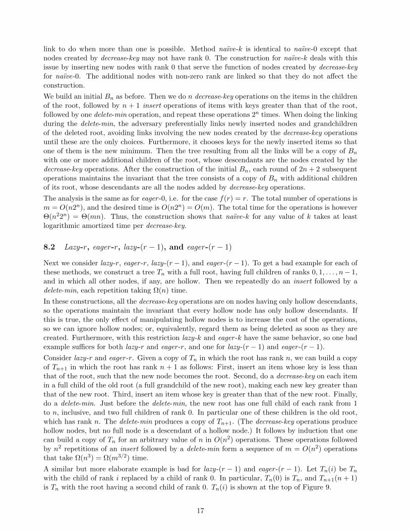
A similar but more elaborate example is bad for lazy-(r − 1) and eager -(r − 1). Let Tn(i) be Tnwith the child of rank i replaced by a child of rank 0. In particular, Tn(0) is Tn, and Tn+1(n + 1)is Tn with the root having a second child of rank 0. Tn(i) is shown at the top of Figure 9.

17

Tn(i)

· · · · · ·

n− 1 n− 2 i+ 1 0 i− 1 0

· · · x

n− 1 n− 2 i+ 1 i

· · ·

i− 1 i− 2 0

Figure 9: The construction for lazy-(r−1) and eager -(r−1). Only full nodes are shown. Solid andsquiggly lines denote edges formed by ranked and unranked links, respectively. Ranks are shownbeneath nodes. (Top) The tree Tn(i). (Bottom) The tree obtained from Tn(i) by inserting an itemand performing a delete-min operation.

Given a copy of Tn(i) with i > 0, we can build a copy of Tn(i− 1) as follows: First, insert an itemwhose key is greater than that of the root but less than that of all other items. Now the root hasthree children of rank 0. Second, do a delete-min. The just-inserted node will become the root, theother children of the old root having rank less than i will be linked by ranked links to form a treewhose root x has rank i and is a child of the new root, and the remaining children of the old rootwill become children of the new root. Node x has exactly one full proper descendant of each rankfrom 0 to i− 1, inclusive. The tree obtained after performing the delete-min operation is shown atthe bottom of Figure 9. (In the figure we assume that the key of the child of the old root of rankj < i is smaller than the key of the child of the old root of rank j − 1 for every 1 ≤ j < i. In thiscase x is the child of rank i− 1 of the old root and its children after the delete-min are the childrenof the old root of rank ≤ i − 2. But unlike the situation shown in the figure, the descendants ofx can in general be linked arbitrarily.) Finally, do a decrease-key on each of the items in the fullproper descendants of x in a bottom-up order (so that each decrease-key is on an item in a nodewith only hollow descendants), making each new key greater than that of the root. The rank ofeach new node created this way is 1 smaller than the rank of the node it came from, except for thenode that already has rank 0. The root thus gets two new children of rank 0 and one new child ofeach rank from 1 to i− 2. The result is a copy of Tn(i− 1), with some extra hollow nodes, whichwe ignore. We can convert a copy of Tn(0) = Tn into a copy of Tn+1(n + 1) by inserting a newitem with key greater than that of the root. It follows by induction that one can build a copy of Tnin m = O(n3) operations. These operations followed by n3 repetitions of an insert followed by adelete-min take a total of Ω(n4) = Ω(m4/3) time but the desired time is O(n3 log n) = O(m logm).

18

8.3 Lazy-k

Finally, we consider lazy-k for any k in the small regime. We again construct a tree for which wecan repeat an expensive sequence of operations. We first give a construction for lazy-0 and thenshow how to generalize the construction to all choices of k in the small regime.

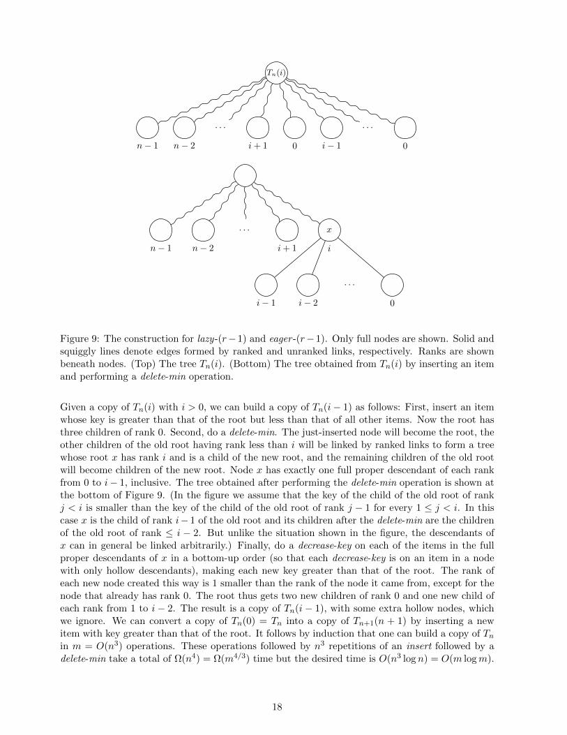
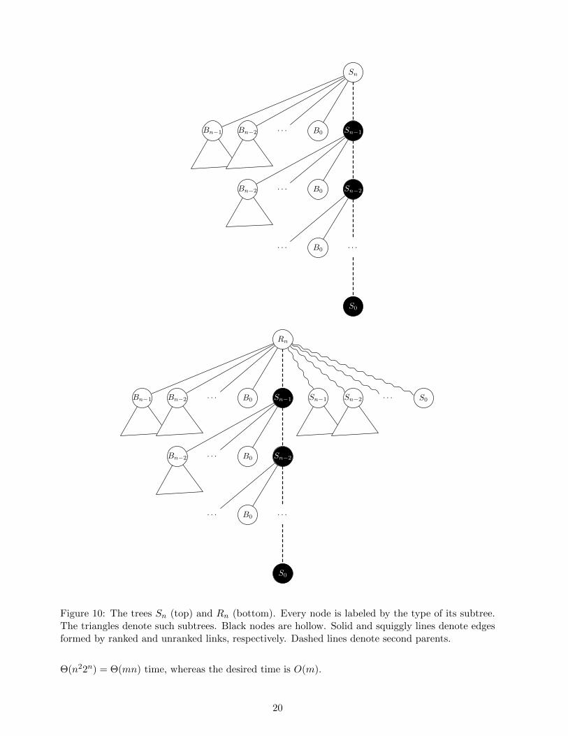
Define the tree Sn inductively as follows. Tree S0 is a single node. For n > 0, Sn is a tree witha full root of rank n, having one hollow child that is the root of Sn−1 and having full children ofranks 0, 1, . . . , n − 1, with the i-th full child being the root of a copy of Bi. The tree Sn is shownat the top of Figure 10. Let Rn be a tree obtained by linking copies of S0, S1, . . . , Sn−1 to Sn, withthe root of Sn winning every link. The tree Rn is shown at the bottom of Figure 10. We showhow to build a copy of Rn for any n. Then we show how to do an expensive sequence of operationsthat starts with a copy of Rn and produces a new one. By building one Rn and then doing enoughrepetitions of the expensive sequence of operations, we get a bad example.

To build a copy of Rn for arbitrary n, we build a related tree Qn that consists of a root whosechildren are the roots of copies of S0, S1, . . . , Sn, with the root of Sn having the smallest key amongthe children of the root of Qn. We obtain Rn from Qn by doing a delete-min.

We build Q0, Q1, . . . , Qn in succession. Tree Q0 is just a node with one full child of rank 0,obtainable by a make-heap and two insert operations. Given Qj , we obtain Qj+1 by a variantof the construction for eager -0. Let xi be the root of the existing copy of Si for i = 0, . . . , j.In the following, all new keys are greater than the key of the root, so that the root remains thesame throughout the sequence of operations. First we do decrease-key operations on the rootsx0, x1, . . . , xj of the existing copies of S0, S1, . . . , Sj . For i = 0, . . . , j, the node xi is thus madehollow and becomes a child of a new node yi of rank 0. Note that a copy of Si+1 can be obtainedfrom repeated, ranked linking of yi and 2i+1 − 1 nodes of rank 0 where yi wins every link in whichit participate. We next do enough insert operations to provide the nodes to build S1, S2, . . . , Sj+1

in this way. The total number of nodes needed is∑j

i=0(2i+1 − 1). Finally, we do two additional

insert operations, followed by a delete-min. The two extra nodes are for a copy of S0 and for a newroot when the old root is deleted.

Deletion of hollow roots by delete-min makes yi the only parent of xi for all i = 0, . . . , j. We areleft with a collection of 1 +

∑j+1i=0 2i roots of rank 0. We do ranked links to build the needed copies

of S0, S1, . . . , Sj+1 in decreasing order. Finally, we link the new root with each of the roots of thenew copies of Si.

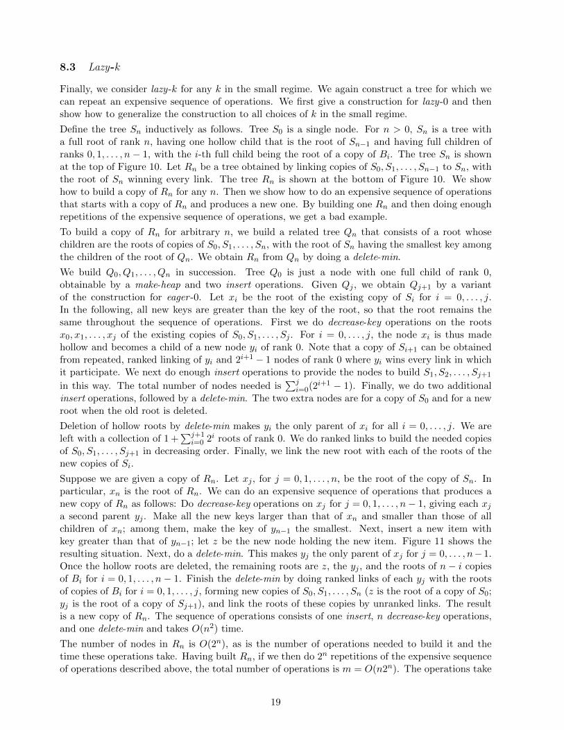
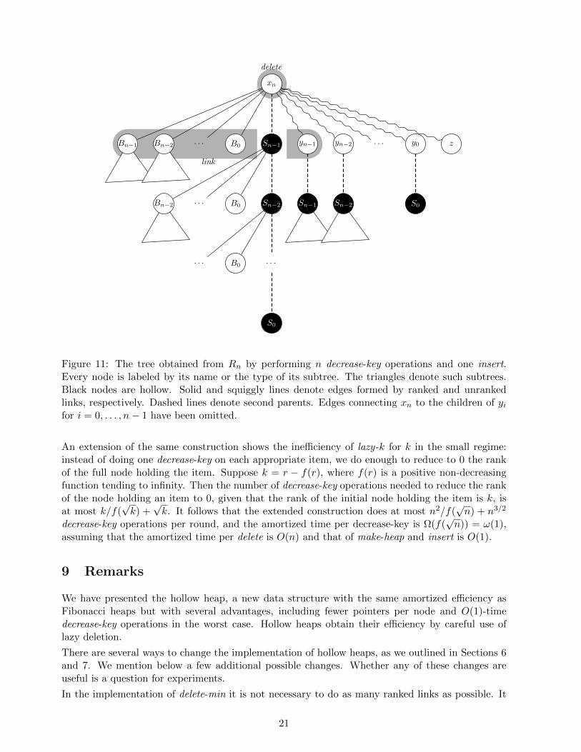
Suppose we are given a copy of Rn. Let xj , for j = 0, 1, . . . , n, be the root of the copy of Sn. Inparticular, xn is the root of Rn. We can do an expensive sequence of operations that produces anew copy of Rn as follows: Do decrease-key operations on xj for j = 0, 1, . . . , n− 1, giving each xja second parent yj . Make all the new keys larger than that of xn and smaller than those of allchildren of xn; among them, make the key of yn−1 the smallest. Next, insert a new item withkey greater than that of yn−1; let z be the new node holding the new item. Figure 11 shows theresulting situation. Next, do a delete-min. This makes yj the only parent of xj for j = 0, . . . , n− 1.Once the hollow roots are deleted, the remaining roots are z, the yj , and the roots of n− i copiesof Bi for i = 0, 1, . . . , n− 1. Finish the delete-min by doing ranked links of each yj with the rootsof copies of Bi for i = 0, 1, . . . , j, forming new copies of S0, S1, . . . , Sn (z is the root of a copy of S0;yj is the root of a copy of Sj+1), and link the roots of these copies by unranked links. The resultis a new copy of Rn. The sequence of operations consists of one insert, n decrease-key operations,and one delete-min and takes O(n2) time.

The number of nodes in Rn is O(2n), as is the number of operations needed to build it and thetime these operations take. Having built Rn, if we then do 2n repetitions of the expensive sequenceof operations described above, the total number of operations is m = O(n2n). The operations take

19

Sn

Bn−1 Bn−2 · · · B0 Sn−1

Bn−2 · · · B0 Sn−2

· · · · · ·B0

S0

Rn

Bn−1 Bn−2 · · · B0 Sn−1 Sn−1 Sn−2 · · · S0

Bn−2 · · · B0 Sn−2

· · · · · ·B0

S0

Figure 10: The trees Sn (top) and Rn (bottom). Every node is labeled by the type of its subtree.The triangles denote such subtrees. Black nodes are hollow. Solid and squiggly lines denote edgesformed by ranked and unranked links, respectively. Dashed lines denote second parents.

Θ(n22n) = Θ(mn) time, whereas the desired time is O(m).

20

link

delete

xn

Bn−1 Bn−2 · · · B0 Sn−1 yn−1 yn−2 · · · y0 z

Sn−1 Sn−2 S0Bn−2 · · · B0 Sn−2

· · · · · ·B0

S0

Figure 11: The tree obtained from Rn by performing n decrease-key operations and one insert.Every node is labeled by its name or the type of its subtree. The triangles denote such subtrees.Black nodes are hollow. Solid and squiggly lines denote edges formed by ranked and unrankedlinks, respectively. Dashed lines denote second parents. Edges connecting xn to the children of yifor i = 0, . . . , n− 1 have been omitted.

An extension of the same construction shows the inefficiency of lazy-k for k in the small regime:instead of doing one decrease-key on each appropriate item, we do enough to reduce to 0 the rankof the full node holding the item. Suppose k = r − f(r), where f(r) is a positive non-decreasingfunction tending to infinity. Then the number of decrease-key operations needed to reduce the rankof the node holding an item to 0, given that the rank of the initial node holding the item is k, isat most k/f(

√k) +

√k. It follows that the extended construction does at most n2/f(

√n) + n3/2

decrease-key operations per round, and the amortized time per decrease-key is Ω(f(√n)) = ω(1),

assuming that the amortized time per delete is O(n) and that of make-heap and insert is O(1).

9 Remarks

We have presented the hollow heap, a new data structure with the same amortized efficiency asFibonacci heaps but with several advantages, including fewer pointers per node and O(1)-timedecrease-key operations in the worst case. Hollow heaps obtain their efficiency by careful use oflazy deletion.

There are several ways to change the implementation of hollow heaps, as we outlined in Sections 6and 7. We mention below a few additional possible changes. Whether any of these changes areuseful is a question for experiments.

In the implementation of delete-min it is not necessary to do as many ranked links as possible. It

21

suffices to find a maximum matching of roots of the same rank, link the matched roots by rankedlinks, and link the remaining roots by unranked links. See [11].

As in Fibonacci heaps, it suffices to do ranked links only. A heap is represented by a set of treesinstead of a single tree, with a pointer to a root of minimum key. When deleting the item in a root,ranked links are done until no more are possible; then the remaining roots are scanned to find oneof minimum key. As mentioned in Section 7, using this idea in eager hollow heaps allows one torepresent each set of children by a non-circular singly linked list, which simplifies linking.

An extension of this idea is to do all the links in find-min instead of in delete. Again a heap isrepresented by a set of trees rather than a single tree, but with no pointer to a root of minimumkey. A delete operation merely deletes the appropriate item, making the node holding it hollow. Afind-min deletes hollow roots and does links until there is only one root, a full one, or does rankedlinks until none is possible.

References

[1] G.S. Brodal. Worst-case efficient priority queues. In Proceedings of the 7th ACM-SIAM Sym-posium on Discrete Algorithms (SODA), pages 52–58, 1996.

[2] G.S. Brodal, G. Lagogiannis, and R.E. Tarjan. Strict Fibonacci heaps. In Proceedings of the44th ACM Symposium on Theory of Computing (STOC), pages 1177–1184, 2012.

[3] M.R. Brown. Implementation and analysis of binomial queue algorithms. SIAM Journal onComputing, 7(3):298–319, 1978.

[4] T.M. Chan. Quake heaps: A simple alternative to Fibonacci heaps. In Space-Efficient DataStructures, Streams, and Algorithms, pages 27–32, 2013.

[5] E.W. Dijkstra. A note on two problems in connexion with graphs. Numerische Mathematik,1:269–271, 1959.

[6] J.R. Driscoll, H.N. Gabow, R. Shrairman, and R.E. Tarjan. Relaxed heaps: an alternativeto Fibonacci heaps with applications to parallel computation. Communications of the ACM,31(11):1343–1354, 1988.

[7] J. Edmonds. Optimum branchings. J. Res. Nat. Bur. Standards, 71B:233–240, 1967.

[8] A. Elmasry. The violation heap: a relaxed Fibonacci-like heap. Discrete Math., Alg. and Appl.,2(4):493–504, 2010.

[9] M.L. Fredman and R.E. Tarjan. Fibonacci heaps and their uses in improved network opti-mization algorithms. Journal of the ACM, 34(3):596–615, 1987.

[10] H.N. Gabow, Z. Galil, T.H. Spencer, and R.E. Tarjan. Efficient algorithms for finding minimumspanning trees in undirected and directed graphs. Combinatorica, 6:109–122, 1986.

[11] B. Haeupler, S. Sen, and R.E. Tarjan. Rank-pairing heaps. SIAM Journal on Computing,40(6):1463–1485, 2011.

[12] P. Høyer. A general technique for implementation of efficient priority queues. In Proceedingsof the 3rd Israeli Symposium on the Theory of Computing and Systems (ISTCS), pages 57–66,1995.

22

[13] H. Kaplan, N. Shafrir, and R.E. Tarjan. Meldable heaps and boolean union-find. In Proceedingsof the 34th ACM Symposium on Theory of Computing (STOC), pages 573–582, 2002.

[14] H. Kaplan and R.E. Tarjan. Thin heaps, thick heaps. ACM Transactions on Algorithms,4(1):1–14, 2008.

[15] H. Kaplan, R.E. Tarjan, and U. Zwick. Fibonacci heaps revisited. CoRR, abs/1407.5750, 2014.

[16] D.E. Knuth. Sorting and searching, volume 3 of The art of computer programming. Addison-Wesley, second edition, 1998.

[17] G.L. Peterson. A balanced tree scheme for meldable heaps with updates. Technical ReportGIT-ICS-87-23, School of Informatics and Computer Science, Georgia Institute of Technology,Atlanta, GA, 1987.

[18] R. C. Prim. Shortest connection networks and some generalizations. Bell System TechnicalJournal, 36:1389–1401, 1957.

[19] T. Takaoka. Theory of 2-3 heaps. Discrete Applied Mathematics, 126(1):115–128, 2003.

[20] R.E. Tarjan. Data structures and network algorithms. SIAM, 1983.

[21] J. Vuillemin. A data structure for manipulating priority queues. Communications of the ACM,21:309–314, 1978.

23