arX

iv:1

401.

0261

v2 [

hep-

th]

6 A

pr 2

014

Holographic Renyi entropy in AdS3/LCFT2

correspondence

Bin Chen1,2,3,4∗, Feng-yan Song1†and Jia-ju Zhang1‡

1Department of Physics and State Key Laboratory of Nuclear Physics and Technology,

Peking University, 5 Yiheyuan Rd, Beijing 100871, P. R. China2Collaborative Innovation Center of Quantum Matter, 5 Yiheyuan Rd, Beijing 100871, P. R. China3Center for High Energy Physics, Peking University, 5 Yiheyuan Rd, Beijing 100871, P. R. China

4Beijing Center for Mathematics and Information Interdisciplinary Sciences,

105 W 3rd Ring Rd N, Beijing 100048, P. R. China

Abstract

The recent study in AdS3/CFT2 correspondence shows that the tree level contribution and1-loop correction of holographic Renyi entanglement entropy (HRE) exactly match the direct CFTcomputation in the large central charge limit. This allows the Renyi entanglement entropy to be anew window to study the AdS/CFT correspondence. In this paper we generalize the study of Renyientanglement entropy in pure AdS3 gravity to the massive gravity theories at the critical points.For the cosmological topological massive gravity (CTMG), the dual conformal field theory (CFT)could be a chiral conformal field theory or a logarithmic conformal field theory (LCFT), dependingon the asymptotic boundary conditions imposed. In both cases, by studying the short intervalexpansion of the Renyi entanglement entropy of two disjoint intervals with small cross ratio x, wefind that the classical and 1-loop HRE are in exact match with the CFT results, up to order x6. Tothis order, the difference between the massless graviton and logarithmic mode can be seen clearly.Moreover, for the cosmological new massive gravity (CNMG) at critical point, which could be dualto a logarithmic CFT as well, we find the similar agreement in the CNMG/LCFT correspondence.Furthermore we read the 2-loop correction of graviton and logarithmic mode to HRE from CFTcomputation. It has distinct feature from the one in pure AdS3 gravity.

∗bchen01@pku.edu.cn†songfy@pku.edu.cn‡jjzhang@pku.edu.cn

Contents

1 Introduction 2

2 Holographic Renyi entropy in critical massive gravity 5

2.1 CTMG at critical point . . . . . . . . . . . . . . . . . . . . . . . . . . . . . . . . . . . 7

2.2 Critical CNMG . . . . . . . . . . . . . . . . . . . . . . . . . . . . . . . . . . . . . . . . 9

3 Renyi entropy in LCFT 11

3.1 Basics of LCFT . . . . . . . . . . . . . . . . . . . . . . . . . . . . . . . . . . . . . . . . 11

3.2 Short interval expansion of Renyi entropy . . . . . . . . . . . . . . . . . . . . . . . . . 13

3.3 LCFT dual to critical CTMG . . . . . . . . . . . . . . . . . . . . . . . . . . . . . . . . 15

3.4 LCFT dual to critical CNMG . . . . . . . . . . . . . . . . . . . . . . . . . . . . . . . . 19

4 Conclusion and discussion 21

A Some useful formulas 23

1 Introduction

Entanglement entropy has been under active study in the past decade. It is defined as the von

Neumann entropy of reduced density matrix ρA of a subsystem A

SA = −TrAρA log ρA. (1.1)

For a quantum field theory, the entanglement entropy is called the geometric entropy as the leading

contribution is proportional to the area of the boundary of the subsystem [1,2]. More generally, with

the reduced density matrix, one may define the Renyi entanglement entropy as

S(n)A = − 1

n− 1log TrAρ

nA. (1.2)

It is easy to see that the entanglement entropy and the Renyi entropy are related by

SA = limn→1

S(n)A . (1.3)

One can also define the Renyi mutual information of two subsystems A and B as

I(n)A,B = S

(n)A + S

(n)B − S

(n)A∪B. (1.4)

From its definition, the Renyi entropy could be calculated via the replica trick [3]. However, this trick

leads to the computation of the partition function on a spacetime manifold with nontrivial topology.

For example, in two-dimensional quantum field theory on complex plane, the n-th Renyi entropy of N

intervals requires a partition function on a Riemann surface of genus (n − 1)(N − 1). Therefore even

though the Renyi entropy is easier than the entanglement entropy, it is still quite hard to compute in

practice.

2

The AdS/CFT correspondence provides an effective tool to study the entanglement and the Renyi

entropies. It was firstly proposed by Ryu and Takayanagi [4, 5] that the entanglement entropy of

subregion A in a conformal field theory (CFT) could be holographically given by the area of a minimal

surface which is homogeneous to A in the dual AdS gravity. This so-called holographic entanglement

entropy has been studied intensely since its proposal, see good reviews [6, 7] for complete references.

For the Renyi entropy, it could be calculated holographically in a similar way [8,9]. Very recently the

RT formula or prescription has been proved from various points of view. In [10, 11] the RT formula

has been proved in AdS3/CFT2 case. For general case, the RT formula has been shown to be true

from the point of view of the generalized gravitational entropy [12]1. One essential point in these

proofs is to find the gravitational configurations in applying the replica trick. This turns out to be

a subtle issue and has not been well-understood in general cases. However, in AdS3/CFT2 case,

the bulk gravitational configurations ending on a higher-genus Riemann surface can be constructed

explicitly without trouble. Then the Euclidean gravity action of the configuration gives the leading

contribution to the holographic Renyi entropy (HRE). Moreover, with the gravitational configuration,

the gravitational 1-loop correction has been considered in [15]. This 1-loop quantum correction is

essential to the mutual information [16]. From AdS3/CFT2 correspondence for pure AdS gravity, the

central charge c = 3l2G is inversely proportional to the Newton coupling constant G, so the large central

charge c limit corresponds to the weak coupling limit in the gravity. Therefore the classical, quantum

1-loop, 2-loop, ... contributions to HRE correspond to the CFT contributions proportional to c, c0,

1c, ..., respectively [8]. It is remarkable that for the two-interval case with a small cross ratio x, the

classical and 1-loop contributions to the HRE are in exact agreement with the CFT results up to

order x8 [17,18]. These facts provide nontrivial support of the holographic computations of the Renyi

entropy, not only at the classical level but also at quantum 1-loop level.

On the other hand, the Renyi entropy could be taken as a new window to study the AdS3/CFT2

correspondence. For the two-interval case, the second Renyi entropy is actually the torus partition

function, which is usually the first check on the possible correspondence. The higher rank Renyi

entropy is in general hard to compute, but could be calculated order by order by using the operator

product expansion of the twist operators in the small interval limit [8, 17–20]. In [17], we considered

the pure AdS3 gravity and the vacuum Verma module of its CFT dual, and found exact agreements.

Recently such investigation has been generalized to the holographic Renyi entropy for Higher spin

gravity/CFT with W symmetry correspondence in [18, 20]. In this paper, we would like to extend

our study to the topologically massive gravity with negative cosmological constant (CTMG) [21, 22]

and cosmologically new massive gravity (CNMG) [23, 24], both of which at critical points have been

conjectured to be dual to some kinds of CFT under appropriate asymptotic boundary conditions.

In three dimensional (3D) topologically massive gravity (TMG) with a negative cosmological con-

stant, there is a gravitational Chern-Simons term in the action. Off the critical point, there could be

a massive fluctuation around the AdS3 vacuum, besides two massless modes. It turns out that off the

1For earlier efforts to prove RT formula, see for examples [13,14].

3

critical point the theory is ill-defined due to the negative energy of the massive mode. At the critical

points, the theory could be well-defined but becomes chiral after imposing Brown-Henneaux boundary

conditions, as the local massive mode becomes degenerate with the left massless mode and the only

degree of freedom is a massless boundary graviton. It was conjectured that the chiral gravity is dual

to a chiral CFT with only right-mover [25,26]. However, even at the critical point, there is actually a

logarithmic mode [27–29], if one does not impose the Brown-Henneaux boundary conditions. More-

over it has been found that there exist another set of consistent boundary conditions to include the

logarithmic mode, and the resulting quantum gravity is proposed to be dual to a logarithmic CFT

(LCFT) [30–34]. The lesson is that the quantum gravity is defined with respect to the asymptotic

boundary conditions.

Another interesting class of 3D massive gravity is the so-called new massive gravity (NMG). Due

to the presence of the higher derivative terms, the theory generically has massive gravitons, similar

to CTMG. In this work, we focus on the AdS vacuum, in which NMG is called cosmological NMG

(CNMG). For CNMG, there exists a critical point where the massive modes disappear and the loga-

rithmic modes appear [24, 35]. Very interestingly, similar to CTMG, there are more than one set of

consistent boundary conditions to define the quantum gravity. In general, one may impose the usual

Brown-Henneaux boundary conditions to set up a AdS3/CFT2 correspondence, but at critical point

there could be other sets of consistent boundary conditions to include the logarithmic mode(s) [36].

Therefore at the critical point, there is a CNMG/LCFT correspondence [34, 37], even though the

central charges in this case are vanishing.

In this work, we study the Renyi entropy of two disjoint intervals in the framework of CTMG/CFT

correspondence. We show that for a general gravity theory with a AdS3 vacuum, the classical HRE is

similar to the one in pure AdS gravity

∂Sn

∂zi= −n(cL + cR)

12γi, (1.5)

with the only difference on the sum of the central charges of the dual CFT. For the CTMG, as the sum

of the central charges is the same as the pure AdS gravity, so is the classical HRE. However we find

that the 1-loop quantum corrections depend on the choice of asymptotic boundary conditions. On the

other side, we compute the OPE of twist operators in the small interval limit in the corresponding

CFT duals. For the chiral CFT, the computation is relatively easy, but for the logarithmic CFT, we

have to treat it carefully. In both the chiral and logarithmic cases, we find that HRE and CFT results

are in exact agreement up to order x6. We furthermore discuss the holographic Renyi entropy in

CNMG at the critical point. In this case, the classical contribution to the entropy is simply vanishing

as the central charges are zero, but the quantum corrections are not vanishing. We find agreement

in the CNMG/LCFT correspondence as well. Our results support the correspondence between the

three-dimensional critical massive gravity and two-dimensional logarithmic CFT.

The remaining of the paper is arranged as follows. In Section 2 we review the fundamental facts

on the chiral gravity and log gravity in the context of CTMG. Then we compute the holographic

4

Renyi entropy in CTMG and CNMG at critical points. In Section 3 after introducing the logarithmic

CFT and showing how to study the OPE of twist operators in it, we compute the Renyi entropy in

the small interval limit carefully. In Section 4, we end with conclusion and discussion. We put some

summation formulas into Appendix A.

Note added While we are finishing the manuscript, there appeared a paper [20], which has some

overlaps with Section 2 of the present work.

2 Holographic Renyi entropy in critical massive gravity

We are going to compute the holographic Renyi entropy in cosmological massive gravity at the critical

point for two intervals with small cross ratio in CFT. As we are considering the entanglement entropy

in the vacuum state of CFT, we focus on the AdS3 vacuum. The classical solutions found in pure AdS3

gravity are always the solutions of these theories. Thus the gravitational configurations corresponding

to the n-th Renyi entropy are the same as the ones worked out in [11,15]. They are just the quotient

of AdS3 by the Schottky group. Locally they are diffeomorphic to global AdS3, or in other words they

satisfy the relations Rµν = 13gµνR = − 2

l2gµν with l being the AdS radius.

The tree level contribution comes from the Euclidean action of the configurations, including the

boundary terms. Here we may consider a quite general 3D gravity theory with a AdS3 vacuum. Let

us start from the Euclidean action

I =1

16πG

∫

d3x√gL(gµν ,∇µ, Rµν) + Ibndy, (2.1)

and forget about the gravitational Chern-Simons terms for a while. The boundary term Ibndy is not

essential in the following discussion. The AdS3 vacuum is of the radius l, which should be determined

from the equation of motion of the theory. In Euclidean gravity, the vacuum becomes a hyperbolic

space H, whose metric could be written in terms of Poincare coordinates as

ds2 =l2

z2(dx2 + dy2 + dz2). (2.2)

The boundary of H is a Riemann sphere at z = 0. The boundary of the above mentioned gravitational

configurations are Riemann surfaces, which could be taken as the quotients of the Riemann sphere by

the Schottky groups.

The bulk action for any gravitational configuration above is

Ibulk =Lm

16πG

∫

d3x√g, (2.3)

where Lm is the value of the Lagrangian density at the AdS vacuum, and is a constant. This action

is obviously divergent and needs regularization. The standard way is to introduce a plane at z = ǫ.

Then the quadratic divergence could be cancelled by the boundary action, i.e.

Iǫ =Lm

16πG(Vǫ −

l

2Aǫ)

=Lml3

16G(Vreg − (2g − 2) ln ǫ), (2.4)

5

where g is the genus of the Riemann surface at the boundary. The logarithmic term could not be

canceled by a local counter term. It is actually related to the Weyl anomaly of a Riemann surface of

genus g [38]. This allows us to determine the central charge of the dual CFT

c =3Lml3

8G, (2.5)

which has been found from another point of view in [39]. More interestingly, it turns out that the

regularized action Iǫ is related to the Liouville action of the Riemann surface [40]. A careful study

along the line in [11] shows that the regularized action could be expressed in terms of the accessory

parameters characterizing the Schottky uniformization,

∂Sn

∂zi= −cn

6γi, (2.6)

where γi is fixed by the monodromy problem of an ordinary differential equation. Therefore for any

3D gravity with a AdS3 vacuum, the classical HRE could be determined by this formula. The only

difference is on the central charge.

If the theory includes the gravitational Chern-Simons term, it does not change the above argument.

The presence of the CS term may induce diffeomorphism anomaly in the stress tensor, but the sum of

the central charges are invariant [41,42]. As a result, the above relation should be modified a little bit

∂Sn

∂zi= −n(cL + cR)

12γi. (2.7)

Note that for a Minkowski 2D CFT the left- and right-moving central charges are denoted by cL,R,

which are just the holomorphic and antiholomorphic central charges c, c for the Euclidean version of

the CFT. For the case of two intervals with small cross ratio x, one can get the classical part of the

holographic Renyi mutual information to order x6 [10, 11,15]

Icln =(c+ c)(n − 1)(n+ 1)2x2

288n3+

(c+ c)(n − 1)(n + 1)2x3

288n3

+(c+ c)(n − 1)(n + 1)2

(

1309n4 − 2n2 − 11)

x4

414720n7

+(c+ c)(n − 1)(n + 1)2

(

589n4 − 2n2 − 11)

x5

207360n7(2.8)

+(c+ c)(n − 1)(n + 1)2

(

805139n8 − 4244n6 − 23397n4 − 86n2 + 188)

x6

313528320n11+O(x7).

For CTMG theory, the sum of the central charges are the same as the pure AdS3 vacuum. Thus the

classical HRE is the same as the one in pure AdS3 gravity.

Note that the above discussion has nothing to do with the choice of the asymptotic boundary

conditions. And the result is true for any AdS3 vacuum, not restricted to the critical points. Therefore

the classical HRE takes a universal form, depending only on the central charges.

For the 1-loop correction to the HRE, the situation is more complex. We have to consider all

the possible fluctuations around the gravitational configurations. As these configurations are locally

diffeomorphic to AdS3, we can study the linearized equation around the AdS vacuum to read the

6

fluctuations. Another closely related subtle issue is the imposing of asymptotic boundary conditions,

since different boundary conditions define different quantum gravities and their CFT duals. In this

section, we discuss two kinds of massive gravity theories at the critical points and the 1-loop correction

to the holographic Renyi entropy in these theories.

2.1 CTMG at critical point

The topologically massive gravity (TMG) has been studied for a long time. From the view of

AdS/CFT, the CFT dual to CTMG has different central charges on the left and right sector due

to the existence of diffeomorphism anomaly. The action of CTMG is

S =1

16πG

∫

d3x√−g

[

R+2

l2+

1

µǫλµνΓρ

σλ(∂µΓσρν +

2

3ΓσκµΓ

κρν)

]

. (2.9)

Here l is AdS radius and G is the Newton constant. We follow the convention that G is positive and

µl ≥ 1 such that the energy of the BTZ black hole is positive and the central charges are always

positive. The AdS3 spacetime is the solution of CTMG

ds2 = l2(

−(

dx+)2 −

(

dx−)2 − 2 cosh(2ρ)dx+dx− + dρ2

)

. (2.10)

The linear fluctuations around the AdS3 vacuum obey a third order differential equation. As a result

if µl 6= 1, there are two massless boundary gravitons hL, hR and a local massive graviton hM . When

µl = 1, the local massive mode becomes degenerate with the left massless mode so that the only degree

of freedom could be the right massless boundary graviton hR. However, there is actually a new mode

at critical point µl = 1, defined by

hlog = limµl→1

hM − hL

µl − 1. (2.11)

This mode has component that increases linearly when ρ goes to infinity, so it is called logarithmic

mode [29]. It satisfies the linearized equation as well, and moreover carries negative energy.

Quantum gravity in AdS3 is defined with respect to the asymptotic boundary conditions. For

CTMG, one may impose the Brown-Henneaux asymptotically boundary conditions [43]

h++ = O(1) h+− = O(1) h+ρ = O(e−2ρ)

h−+ = h+− h−− = O(1) h−ρ = O(e−2ρ)

hρ+ = h+ρ hρ− = h−ρ hρρ = O(e−2ρ)

. (2.12)

Accordingly, the generator of asymptotic symmetry group (ASG) is [26]

Q ∼(

1 +1

µl

)∫

∂Σdx+h++ǫ

+ +

(

1− 1

µl

)∫

∂Σdx−h−−ǫ

−. (2.13)

This set of boundary conditions is well-defined for generic value of µl, and leads to two copies of

Virasoro algebra with the central charges

cL =

(

1− 1

µl

)

3l

2G, cR =

(

1 +1

µl

)

3l

2G. (2.14)

7

At the critical point µl = 1, the generator becomes

Q ∼∫

∂Σdx+h++ǫ

+. (2.15)

There is only one set of Virasoro algebra, corresponding to the right-moving sector of a CFT. Note

that the Brown-Henneaux boundary conditions exclude the logarithmic mode. Therefore the CTMG

theory becomes a chiral gravity at the critical point. It could be holographically dual to a chiral CFT

with pure right sector [25]

cL = 0, cR =3l

G. (2.16)

On the other hand, one can impose another set of consistent boundary conditions to include the

logarithmic mode [30,32]. To make the right-moving charge be well defined, the boundary conditions

should be

h++ = O(1) h+− = O(1) h+ρ = O(e−2ρ)

h−+ = h+− h−− = O(ρ) h−ρ = O(ρe−2ρ)

hρ+ = h+ρ hρ− = h−ρ hρρ = O(e−2ρ)

, (2.17)

under which the left- and right-moving charges QL andQR are both finite. Even though the logarithmic

mode carries negative energy, the CTMG including such mode is conjectured to be dual a logarithmic

CFT with the same central charges (2.16).

In the log gravity, using the method of heat kernel [44, 45], one can read the 1-loop partition

function [34]

Z1−loopTMG =

∞∏

r=2

1

|1− qr|2∞∏

m=2

∞∏

m=0

1

1− qmqm. (2.18)

The first part being the product over r is the contribution from massless boundary gravitons, while

the remaining part is the contribution from the logarithmic mode. According to [15], the on-shell

1-loop partition function could be

logZ1−loopTMG = −

∑

γ∈P

∞∑

r=2

log (|1− qrγ |)−1

2

∑

γ∈P

∞∑

m=2

∞∑

m=0

log (1 − qmγ qmγ ). (2.19)

Here P is a set of representatives of primitive conjugacy classes of the Schottky group Γ. And the qγ

is one of the two eigenvalues of the matrix γ ∈ Γ with the condition that |qγ | < 1. We consider the

case of two short intervals on complex plane with small cross ratio. Using the conformal invariance,

we can map the subsystem to A = (−∞,−1] ∪ [−y, y] ∪ [1,+∞) as in [15], and the cross-ratio will be

x =4y

(1 + y)2. (2.20)

To the order of x6, we only need the so-called consecutively decreasing words (CDWs)

γk,m = Mm+k2 T−1Mk

2 TM−m2 . (2.21)

8

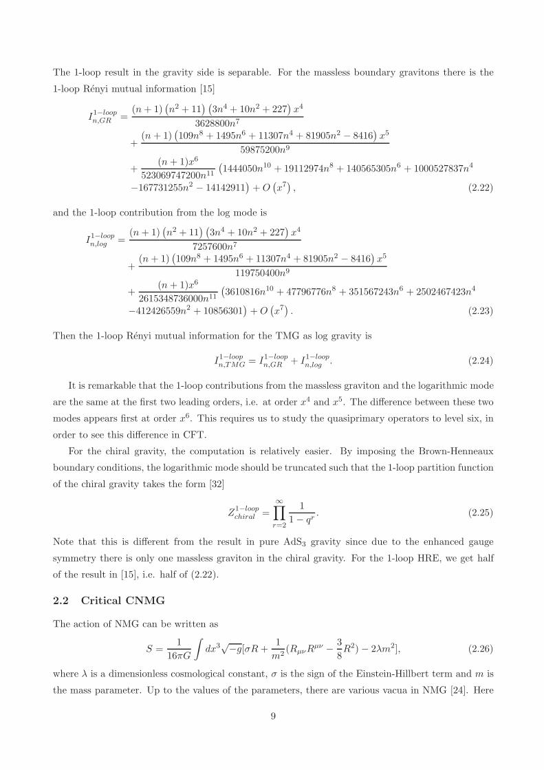
The 1-loop result in the gravity side is separable. For the massless boundary gravitons there is the

1-loop Renyi mutual information [15]

I1−loopn,GR =

(n+ 1)(

n2 + 11) (

3n4 + 10n2 + 227)

x4

3628800n7

+(n + 1)

(

109n8 + 1495n6 + 11307n4 + 81905n2 − 8416)

x5

59875200n9

+(n+ 1)x6

523069747200n11

(

1444050n10 + 19112974n8 + 140565305n6 + 1000527837n4

−167731255n2 − 14142911)

+O(

x7)

, (2.22)

and the 1-loop contribution from the log mode is

I1−loopn,log =

(n+ 1)(

n2 + 11) (

3n4 + 10n2 + 227)

x4

7257600n7

+(n+ 1)

(

109n8 + 1495n6 + 11307n4 + 81905n2 − 8416)

x5

119750400n9

+(n+ 1)x6

2615348736000n11

(

3610816n10 + 47796776n8 + 351567243n6 + 2502467423n4

−412426559n2 + 10856301)

+O(

x7)

. (2.23)

Then the 1-loop Renyi mutual information for the TMG as log gravity is

I1−loopn,TMG = I1−loop

n,GR + I1−loopn,log . (2.24)

It is remarkable that the 1-loop contributions from the massless graviton and the logarithmic mode

are the same at the first two leading orders, i.e. at order x4 and x5. The difference between these two

modes appears first at order x6. This requires us to study the quasiprimary operators to level six, in

order to see this difference in CFT.

For the chiral gravity, the computation is relatively easier. By imposing the Brown-Henneaux

boundary conditions, the logarithmic mode should be truncated such that the 1-loop partition function

of the chiral gravity takes the form [32]

Z1−loopchiral =

∞∏

r=2

1

1− qr. (2.25)

Note that this is different from the result in pure AdS3 gravity since due to the enhanced gauge

symmetry there is only one massless graviton in the chiral gravity. For the 1-loop HRE, we get half

of the result in [15], i.e. half of (2.22).

2.2 Critical CNMG

The action of NMG can be written as

S =1

16πG

∫

dx3√−g[σR+

1

m2(RµνR

µν − 3

8R2)− 2λm2], (2.26)

where λ is a dimensionless cosmological constant, σ is the sign of the Einstein-Hillbert term and m is

the mass parameter. Up to the values of the parameters, there are various vacua in NMG [24]. Here

9

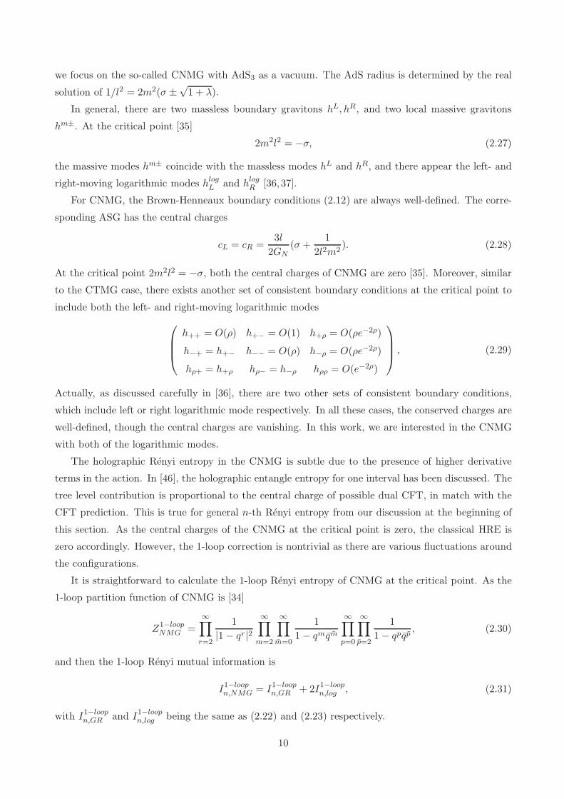
we focus on the so-called CNMG with AdS3 as a vacuum. The AdS radius is determined by the real

solution of 1/l2 = 2m2(σ ±√1 + λ).

In general, there are two massless boundary gravitons hL, hR, and two local massive gravitons

hm±. At the critical point [35]

2m2l2 = −σ, (2.27)

the massive modes hm± coincide with the massless modes hL and hR, and there appear the left- and

right-moving logarithmic modes hlogL and hlogR [36, 37].

For CNMG, the Brown-Henneaux boundary conditions (2.12) are always well-defined. The corre-

sponding ASG has the central charges

cL = cR =3l

2GN(σ +

1

2l2m2). (2.28)

At the critical point 2m2l2 = −σ, both the central charges of CNMG are zero [35]. Moreover, similar

to the CTMG case, there exists another set of consistent boundary conditions at the critical point to

include both the left- and right-moving logarithmic modes

h++ = O(ρ) h+− = O(1) h+ρ = O(ρe−2ρ)

h−+ = h+− h−− = O(ρ) h−ρ = O(ρe−2ρ)

hρ+ = h+ρ hρ− = h−ρ hρρ = O(e−2ρ)

, (2.29)

Actually, as discussed carefully in [36], there are two other sets of consistent boundary conditions,

which include left or right logarithmic mode respectively. In all these cases, the conserved charges are

well-defined, though the central charges are vanishing. In this work, we are interested in the CNMG

with both of the logarithmic modes.

The holographic Renyi entropy in the CNMG is subtle due to the presence of higher derivative

terms in the action. In [46], the holographic entangle entropy for one interval has been discussed. The

tree level contribution is proportional to the central charge of possible dual CFT, in match with the

CFT prediction. This is true for general n-th Renyi entropy from our discussion at the beginning of

this section. As the central charges of the CNMG at the critical point is zero, the classical HRE is

zero accordingly. However, the 1-loop correction is nontrivial as there are various fluctuations around

the configurations.

It is straightforward to calculate the 1-loop Renyi entropy of CNMG at the critical point. As the

1-loop partition function of CNMG is [34]

Z1−loopNMG =

∞∏

r=2

1

|1− qr|2∞∏

m=2

∞∏

m=0

1

1− qmqm

∞∏

p=0

∞∏

p=2

1

1− qpqp, (2.30)

and then the 1-loop Renyi mutual information is

I1−loopn,NMG = I1−loop

n,GR + 2I1−loopn,log , (2.31)

with I1−loopn,GR and I1−loop

n,log being the same as (2.22) and (2.23) respectively.

10

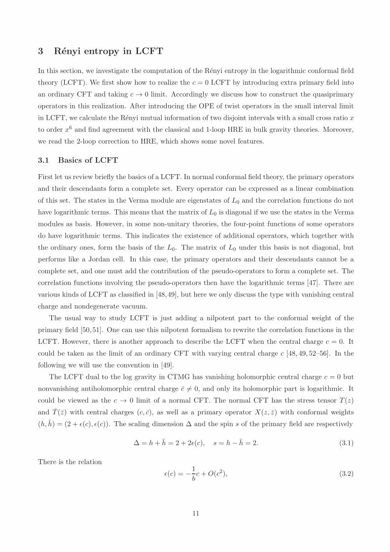
3 Renyi entropy in LCFT

In this section, we investigate the computation of the Renyi entropy in the logarithmic conformal field

theory (LCFT). We first show how to realize the c = 0 LCFT by introducing extra primary field into

an ordinary CFT and taking c → 0 limit. Accordingly we discuss how to construct the quasiprimary

operators in this realization. After introducing the OPE of twist operators in the small interval limit

in LCFT, we calculate the Renyi mutual information of two disjoint intervals with a small cross ratio x

to order x6 and find agreement with the classical and 1-loop HRE in bulk gravity theories. Moreover,

we read the 2-loop correction to HRE, which shows some novel features.

3.1 Basics of LCFT

First let us review briefly the basics of a LCFT. In normal conformal field theory, the primary operators

and their descendants form a complete set. Every operator can be expressed as a linear combination

of this set. The states in the Verma module are eigenstates of L0 and the correlation functions do not

have logarithmic terms. This means that the matrix of L0 is diagonal if we use the states in the Verma

modules as basis. However, in some non-unitary theories, the four-point functions of some operators

do have logarithmic terms. This indicates the existence of additional operators, which together with

the ordinary ones, form the basis of the L0. The matrix of L0 under this basis is not diagonal, but

performs like a Jordan cell. In this case, the primary operators and their descendants cannot be a

complete set, and one must add the contribution of the pseudo-operators to form a complete set. The

correlation functions involving the pseudo-operators then have the logarithmic terms [47]. There are

various kinds of LCFT as classified in [48,49], but here we only discuss the type with vanishing central

charge and nondegenerate vacuum.

The usual way to study LCFT is just adding a nilpotent part to the conformal weight of the

primary field [50,51]. One can use this nilpotent formalism to rewrite the correlation functions in the

LCFT. However, there is another approach to describe the LCFT when the central charge c = 0. It

could be taken as the limit of an ordinary CFT with varying central charge c [48, 49, 52–56]. In the

following we will use the convention in [49].

The LCFT dual to the log gravity in CTMG has vanishing holomorphic central charge c = 0 but

nonvanishing antiholomorphic central charge c 6= 0, and only its holomorphic part is logarithmic. It

could be viewed as the c → 0 limit of a normal CFT. The normal CFT has the stress tensor T (z)

and T (z) with central charges (c, c), as well as a primary operator X(z, z) with conformal weights

(h, h) = (2 + ǫ(c), ǫ(c)). The scaling dimension ∆ and the spin s of the primary field are respectively

∆ = h+ h = 2 + 2ǫ(c), s = h− h = 2. (3.1)

There is the relation

ǫ(c) = −1

bc+O(c2), (3.2)

11

in which the constant b is called the new anomaly. For the LCFT dual to the log gravity there is [33]

b = −3l

G. (3.3)

The operator X could be normalized such that

〈X(z1, z1)X(z2, z2)〉C =αX

z2h12 z2h12

, (3.4)

where zij ≡ zi − zj , and

αX =B(c)

c, B(c) = −1

2+B1c+O(c2). (3.5)

Note that the monodromy of the two-point function requires that s must be an integer or a half

integer. As usual there are two-point functions

〈T (z1)T (z2)〉C =c

2z412,

〈T (z1)X(z2, z2)〉C = 0. (3.6)

The logarithmic partner of T (z) is defined as

t(z, z) =b

cT (z) + bX(z, z). (3.7)

Then one can take the limit c → 0 and get the two-point funtions of the LCFT [49]

〈T (z1)T (z2)〉 = 0, (3.8)

〈T (z1)t(z2, z2)〉 =b

2z412, (3.9)

〈t(z1, z1)t(z2, z2)〉 =B1 − b ln (|z12|2)

z412. (3.10)

Note that the constant B1 can be set to zero with a redefinition of t, and we will adopt B1 = 0

hereafter. In the calculation below we will also need the three-point functions [49]

〈T (z1)X(z2, z2)X(z3, z3)〉C =hαX

z212z213z

2h−223 z2h23

,

〈T (z1)X(z2, z2)X(z3, z3)〉C =hαX

z2h23 z212z

213z

2h−223

,

〈X(z1, z1)X(z2, z2)X(z3, z3)〉C =CXXX

(z12z13z23)h (z12z13z23)

h. (3.11)

The structure constant is

CXXX =D(c)

c2, D(c) = 2− 3

2bc+O(c2). (3.12)

Note that only when s is an even integer can we have CXXX nonvanishing.

The LCFT dual to the critical NMG is a little different to the one dual to the log gravity. In this

case, both the holomorphic and antiholomorphic central charges of the LCFT are zero. And now the

new anomaly is [37]

b = −σ12l

G. (3.13)

12

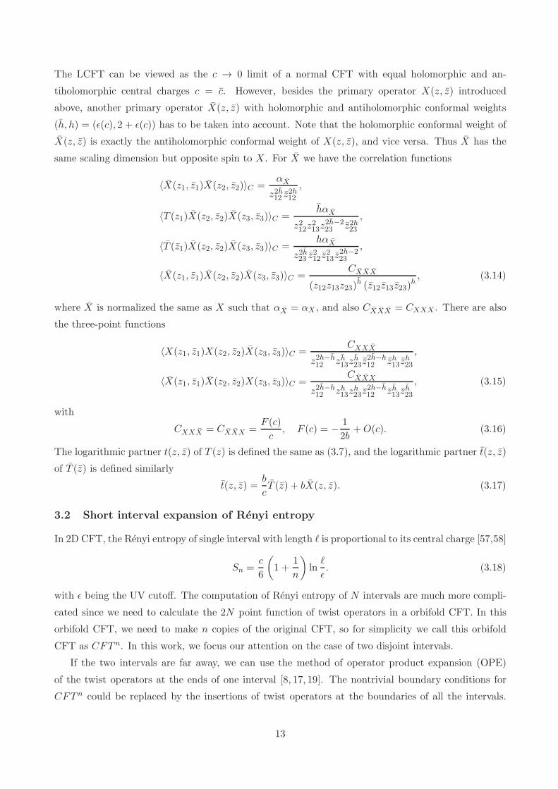
The LCFT can be viewed as the c → 0 limit of a normal CFT with equal holomorphic and an-

tiholomorphic central charges c = c. However, besides the primary operator X(z, z) introduced

above, another primary operator X(z, z) with holomorphic and antiholomorphic conformal weights

(h, h) = (ǫ(c), 2 + ǫ(c)) has to be taken into account. Note that the holomorphic conformal weight of

X(z, z) is exactly the antiholomorphic conformal weight of X(z, z), and vice versa. Thus X has the

same scaling dimension but opposite spin to X. For X we have the correlation functions

〈X(z1, z1)X(z2, z2)〉C =αX

z2h12 z2h12

,

〈T (z1)X(z2, z2)X(z3, z3)〉C =hαX

z212z213z

2h−223 z2h23

,

〈T (z1)X(z2, z2)X(z3, z3)〉C =hαX

z2h23 z212z

213z

2h−223

,

〈X(z1, z1)X(z2, z2)X(z3, z3)〉C =CXXX

(z12z13z23)h (z12z13z23)

h, (3.14)

where X is normalized the same as X such that αX = αX , and also CXXX = CXXX . There are also

the three-point functions

〈X(z1, z1)X(z2, z2)X(z3, z3)〉C =CXXX

z2h−h12 zh13z

h23z

2h−h12 zh13z

h23

,

〈X(z1, z1)X(z2, z2)X(z3, z3)〉C =CXXX

z2h−h12 zh13z

h23z

2h−h12 zh13z

h23

, (3.15)

with

CXXX = CXXX =F (c)

c, F (c) = − 1

2b+O(c). (3.16)

The logarithmic partner t(z, z) of T (z) is defined the same as (3.7), and the logarithmic partner t(z, z)

of T (z) is defined similarly

t(z, z) =b

cT (z) + bX(z, z). (3.17)

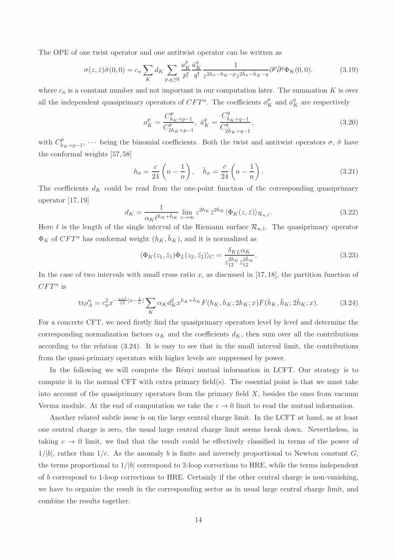
3.2 Short interval expansion of Renyi entropy

In 2D CFT, the Renyi entropy of single interval with length ℓ is proportional to its central charge [57,58]

Sn =c

6

(

1 +1

n

)

lnℓ

ǫ. (3.18)

with ǫ being the UV cutoff. The computation of Renyi entropy of N intervals are much more compli-

cated since we need to calculate the 2N point function of twist operators in a orbifold CFT. In this

orbifold CFT, we need to make n copies of the original CFT, so for simplicity we call this orbifold

CFT as CFT n. In this work, we focus our attention on the case of two disjoint intervals.

If the two intervals are far away, we can use the method of operator product expansion (OPE)

of the twist operators at the ends of one interval [8, 17, 19]. The nontrivial boundary conditions for

CFT n could be replaced by the insertions of twist operators at the boundaries of all the intervals.

13

The OPE of one twist operator and one antitwist operator can be written as

σ(z, z)σ(0, 0) = cn∑

K

dK∑

p,q≥0

apKp!

aqKq!

1

z2hσ−hK−pz2hσ−hK−q∂p∂qΦK(0, 0). (3.19)

where cn is a constant number and not important in our computation later. The summation K is over

all the independent quasiprimary operators of CFT n. The coefficients apK and aqK are respectively

apK =CphK+p−1

Cp2hK+p−1

, aqK =Cq

hK+q−1

Cq

2hK+q−1

, (3.20)

with CphK+p−1, · · · being the binomial coefficients. Both the twist and antitwist operators σ, σ have

the conformal weights [57,58]

hσ =c

24

(

n− 1

n

)

, hσ =c

24

(

n− 1

n

)

. (3.21)

The coefficients dK could be read from the one-point function of the corresponding quasiprimary

operator [17,19]

dK =1

αKℓhK+hK

limz→∞

z2hK z2hK 〈ΦK(z, z)〉Rn,1. (3.22)

Here ℓ is the length of the single interval of the Riemann surface Rn,1. The quasiprimary operator

ΦK of CFT n has conformal weight (hK , hK), and it is normalized as

〈ΦK(z1, z1)ΦL(z2, z2)〉C =δKLαK

z2hK

12 z2hK

12

. (3.23)

In the case of two intervals with small cross ratio x, as discussed in [17,18], the partition function of

CFT n is

trρnA = c2nx− c+c

12(n− 1

n)∑

K

αKd2KxhK+hKF (hK , hK ; 2hK ;x)F (hK , hK ; 2hK ;x). (3.24)

For a concrete CFT, we need firstly find the quasiprimary operators level by level and determine the

corresponding normalization factors αK and the coefficients dK , then sum over all the contributions

according to the relation (3.24). It is easy to see that in the small interval limit, the contributions

from the quasi-primiary operators with higher levels are suppressed by power.

In the following we will compute the Renyi mutual information in LCFT. Our strategy is to

compute it in the normal CFT with extra primary field(s). The essential point is that we must take

into account of the quasiprimary operators from the primary field X, besides the ones from vacuum

Verma module. At the end of computation we take the c → 0 limit to read the mutual information.

Another related subtle issue is on the large central charge limit. In the LCFT at hand, as at least

one central charge is zero, the usual large central charge limit seems break down. Nevertheless, in

taking c → 0 limit, we find that the result could be effectively classified in terms of the power of

1/|b|, rather than 1/c. As the anomaly b is finite and inversely proportional to Newton constant G,

the terms proportional to 1/|b| correspond to 2-loop corrections to HRE, while the terms independent

of b correspond to 1-loop corrections to HRE. Certainly if the other central charge is non-vanishing,

we have to organize the result in the corresponding sector as in usual large central charge limit, and

combine the results together.

14

L0 quasiprimary operators degeneracies

0 1 1

2 Tj n

4Aj n

Tj1Tj2 with j1 < j2n(n−1)

2

5 Jj1j2 with j1 < j2n(n−1)

2

Bj n

Dj n

6 Tj1Aj2 with j1 6= j2 n(n− 1)

Kj1j2 with j1 < j2n(n−1)

2

Tj1Tj2Tj3 with j1 < j2 < j3n(n−1)(n−2)

6

· · · · · · · · ·

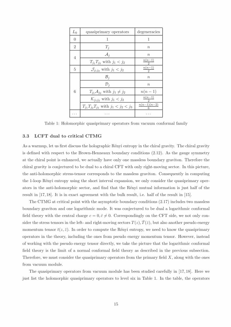
Table 1: Holomorphic quasiprimary operators from vacuum conformal family

3.3 LCFT dual to critical CTMG

As a warmup, let us first discuss the holographic Renyi entropy in the chiral gravity. The chiral gravity

is defined with respect to the Brown-Henneaux boundary conditions (2.12). As the gauge symmetry

at the chiral point is enhanced, we actually have only one massless boundary graviton. Therefore the

chiral gravity is conjectured to be dual to a chiral CFT with only right-moving sector. In this picture,

the anti-holomorphic stress-tensor corresponds to the massless graviton. Consequently in computing

the 1-loop Renyi entropy using the short interval expansion, we only consider the quasiprimary oper-

ators in the anti-holomorphic sector, and find that the Renyi mutual information is just half of the

result in [17,18]. It is in exact agreement with the bulk result, i.e. half of the result in [15].

The CTMG at critical point with the asymptotic boundary conditions (2.17) includes two massless

boundary graviton and one logarithmic mode. It was conjectured to be dual a logarithmic conformal

field theory with the central charge c = 0, c 6= 0. Correspondingly on the CFT side, we not only con-

sider the stress tensors in the left- and right-moving sectors T (z), T (z), but also another pseudo energy

momentum tensor t(z, z). In order to compute the Renyi entropy, we need to know the quasiprimary

operators in the theory, including the ones from pseudo energy momentum tensor. However, instead

of working with the pseudo energy tensor directly, we take the picture that the logarithmic conformal

field theory is the limit of a normal conformal field theory as described in the previous subsection.

Therefore, we must consider the quasiprimary operators from the primary field X, along with the ones

from vacuum module.

The quasiprimary operators from vacuum module has been studied carefully in [17, 18]. Here we

just list the holomorphic quasiprimary operators to level six in Table 1. In the table, the operators

15

are respectively

A = (TT )− 3

10∂2T,

B = (∂T∂T )− 4

5(T∂2T ) +

23

210∂4T,

D = (T (TT ))− 9

10(T∂2T ) +

4

35∂4T +

93

70c+ 29B

Jj1j2 = Tj1i∂Tj2 − i∂Tj1Tj2 ,

Kj1j2 = ∂Tj1∂Tj2 −2

5

(

Tj1∂2Tj2 + ∂2Tj1Tj2

)

. (3.25)

Their normalization constants αK ’s are respectively

α1 = 1, αT =c

2, αA =

c(5c + 22)

10, αB =

36c(70c + 29)

175,

αD =3c(2c − 1)(5c + 22)(7c + 68)

4(70c + 29), αTT =

c2

4, (3.26)

αTA =c2(5c + 22)

20, αTTT =

c3

8, αJ = 2c2, αK =

36c2

5,

and the coefficients dK ’s are respectively

d1 = 1, dT =n2 − 1

12n2, dA =

(n2 − 1)2

288n4, dB = −(n2 − 1)2

(

2n2(35c+ 61) − 93)

10368n6(70c + 29),

dD =(n2 − 1)3

10368n6, dj1j2TT =

1

8n4c

1

s4j1j2+

(n2 − 1)2

144n4, dj1j2TA =

n2 − 1

96n6c

1

s4j1j2+

(n2 − 1)3

3456n6,

dj1j2j3TTT = − 1

8n6c21

s2j1j2s2j2j3

s2j3j1+

n2 − 1

96n6c

(

1

s4j1j2+

1

s4j2j3+

1

s4j3j1

)

+(n2 − 1)3

1728n6,

dj1j2J =1

16n5c

cj1j2s5j1j2

, dj1j2K =5

128n6c

1

s6j1j2− n2 + 9

288n6c

1

s4j1j2− (n2 − 1)2

5184n4. (3.27)

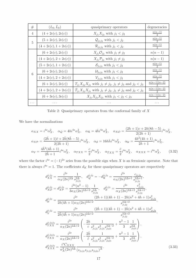
Apart from the quasiprimary operators of CFT n constructed by the operators in the vacuum

conformal family, we also need the ones constructed in terms of X. To level six the additional

quasiprimary operators we need are listed in Table 2. In the table there is the definition

# = limc→0

(

L0 + L0

)

. (3.28)

For the normal CFT we have

O = (TX)− 3

2(2h + 1)∂2X, P = (TX)− 3

2(2h + 1)∂2X, (3.29)

with the normalizations

αO =(2h+ 1)c + 2h(8h − 5)

2(2h + 1)αX , αP =

(2h+ 1)c+ 2h(8h− 5)

2(2h+ 1)αX . (3.30)

For the CFT n we have

Qj1j2 = Xj1i∂Xj2 − i∂Xj1Xj2 , Rj1j2 = Xj1i∂Xj2 − i∂Xj1Xj2 ,

Sj1j2 = Xj1∂∂Xj2 + ∂∂Xj1Xj2 − ∂Xj1 ∂Xj2 − ∂Xj1∂Xj2 ,

Uj1j2 = ∂Xj1∂Xj2 −h

2h+ 1

(

Xj1∂2Xj2 + ∂2Xj1Xj2

)

,

Vj1j2 = ∂Xj1 ∂Xj2 −h

2h+ 1

(

Xj1 ∂2Xj2 + ∂2Xj1Xj2

)

. (3.31)

16

# (L0, L0) quasiprimary operators degeneracies

4 (4 + 2ǫ(c), 2ǫ(c)) Xj1Xj2 with j1 < j2n(n−1)

2

5(5 + 2ǫ(c), 2ǫ(c)) Qj1j2 with j1 < j2

n(n−1)2

(4 + 2ǫ(c), 1 + 2ǫ(c)) Rj1j2 with j1 < j2n(n−1)

2

6

(6 + 2ǫ(c), 2ǫ(c)) Xj1Oj2 with j1 6= j2 n(n− 1)

(4 + 2ǫ(c), 2 + 2ǫ(c)) Xj1Pj2 with j1 6= j2 n(n− 1)

(5 + 2ǫ(c), 1 + 2ǫ(c)) Sj1j2 with j1 < j2n(n−1)

2

(6 + 2ǫ(c), 2ǫ(c)) Uj1j2 with j1 < j2n(n−1)

2

(4 + 2ǫ(c), 2 + 2ǫ(c)) Vj1j2 with j1 < j2n(n−1)

2

(6 + 2ǫ(c), 2ǫ(c)) Tj1Xj2Xj3 with j1 6= j2, j1 6= j3 and j2 < j3n(n−1)(n−2)

2

(4 + 2ǫ(c), 2 + 2ǫ(c)) Tj1Xj2Xj3 with j1 6= j2, j1 6= j3 and j2 < j3n(n−1)(n−2)

2

(6 + 3ǫ(c), 3ǫ(c)) Xj1Xj2Xj3 with j1 < j2 < j3n(n−1)(n−2)

6

· · · · · · · · · · · ·

Table 2: Quasiprimary operators from the conformal family of X

We have the normalizations

αXX = i4sα2X , αQ = 4hi4sα2

X , αR = 4hi4sα2X , αXO =

(2h+ 1)c+ 2h(8h − 5)

2(2h + 1)i4sα2

X ,

αXP =(2h+ 1)c+ 2h(8h− 5)

2(2h+ 1)i4sα2

X , αS = 16hhi4sα2X , αU =

4h2(4h+ 1)

2h+ 1i4sα2

X ,

αV =4h2(4h+ 1)

2h+ 1i4sα2

X , αTXX =c

2i4sα2

X , αTXX =c

2i4sα2

X , αXXX = i4sα3X , (3.32)

where the factor i4s = (−1)2s aries from the possible sign when X is an fermionic operator. Note that

there is always i8s = 1. The coefficients dK for these quasiprimary operators are respectively

dj1j2XX =i2s

αX(2n)2∆1

s2∆j1j2, dj1j2Q = −dj1j2R =

i2s

αX(2n)2∆+1

cj1j2s2∆+1j1j2

,

dj1j2XO = dj1j2XP =i2s(n2 − 1)

3αX(2n)2∆+2

1

s2∆j1j2, dj1j2S =

i2s

αX(2n)2∆+2

c2j1j2s2∆+2j1j2

,

dj1j2U =i2s

2h(4h + 1)αX (2n)2∆+2

(2h+ 1)(4h + 1)− 2h(n2 + 4h+ 1)s2j1j2s2∆+2j1j2

,

dj1j2V =i2s

2h(4h+ 1)αX (2n)2∆+2

(2h+ 1)(4h + 1)− 2h(n2 + 4h+ 1)s2j1j2s2∆+2j1j2

,

dj1j2j3TXX =i2s

αX(2n)2∆+2

(

−2h

c

1

s2j1j2s2j1j3

s2∆−2j2j3

+n2 − 1

3

1

s2∆j2j3

)

,

dj1j2j3TXX

=i2s

αX(2n)2∆+2

(

−2h

c

1

s2j1j2s2j1j3

s2∆−2j2j3

+n2 − 1

3

1

s2∆j2j3

)

,

dj1j2j3XXX =isCXXX

α3X(2n)3∆

1

(sj1j2sj1j3sj2j3)∆. (3.33)

17

Here we have defined sj1j2 ≡ sin π(j1−j2)n

, cj1j2 ≡ cos π(j1−j2)n

, · · · for simplicity. Note that the formulas

(3.32) and (3.33) are general and apply to any nonchiral primary operator X(z, z).

Taking the limit c → 0, we find

αXX

(

dj1j2XX

)2→ 1

(2n)81

s8j1j2, αQ

(

dj1j2Q

)2→ 8

(2n)10c2j1j2s10j1j2

, αR

(

dj1j2R

)2→ 0,

αXO

(

dj1j2XO

)2→ 22(n2 − 1)2

45(2n)121

s8j1j2, αXP

(

dj1j2XP

)2→ c(n2 − 1)2

18(2n)121

s8j1j2, αS

(

dj1j2S

)2→ 0,

αU

(

dj1j2U

)2→ 1

45(2n)12

(

45− 4(n2 + 9)s2j1j2

)2

s12j1j2, αV

(

dj1j2V

)2→ 1

(2n)121

s12j1j2,

αTXX

(

dj1j2j3TXX

)2x2∆+2 → x6

(2n)12

(

1

(sj1j2sj1j3sj2j3)4

(

8

c− 8

b

(

1− 8 log(2nsj2j3) + 4 log x)

)

−4(n2 − 1)

3

1

s2j1j2s2j1j3

s6j2j3

)

αTXX

(

dj1j2j3TXX

)2→ c(n2 − 1)2

18(2n)121

s8j2j3, (3.34)

αXXX

(

dj1j2j3XXX

)2x3∆ → x6

(2n)121

(sj1j2sj1j3sj2j3)4

(

−32

c

+16

b

(

3− 24 log(2n)− 8 log(sj1j2sj2j3sj3j1) + 12 log x)

)

.

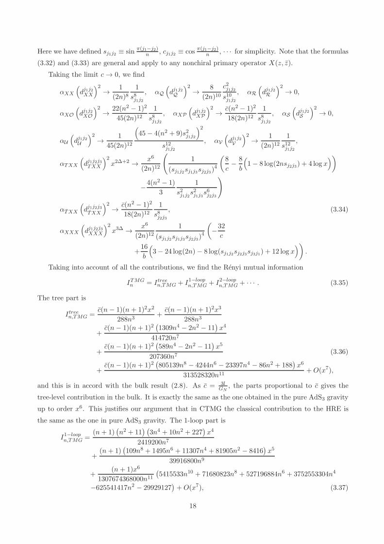
Taking into account of all the contributions, we find the Renyi mutual information

ITMGn = Itreen,TMG + I1−loop

n,TMG + I2−loopn,TMG + · · · . (3.35)

The tree part is

Itreen,TMG =c(n− 1)(n + 1)2x2

288n3+

c(n− 1)(n + 1)2x3

288n3

+c(n− 1)(n + 1)2

(

1309n4 − 2n2 − 11)

x4

414720n7

+c(n− 1)(n + 1)2

(

589n4 − 2n2 − 11)

x5

207360n7(3.36)

+c(n− 1)(n + 1)2

(

805139n8 − 4244n6 − 23397n4 − 86n2 + 188)

x6

313528320n11+O(x7),

and this is in accord with the bulk result (2.8). As c = 3lGN

, the parts proportional to c gives the

tree-level contribution in the bulk. It is exactly the same as the one obtained in the pure AdS3 gravity

up to order x6. This justifies our argument that in CTMG the classical contribution to the HRE is

the same as the one in pure AdS3 gravity. The 1-loop part is

I1−loopn,TMG =

(n+ 1)(

n2 + 11) (

3n4 + 10n2 + 227)

x4

2419200n7

+(n+ 1)

(

109n8 + 1495n6 + 11307n4 + 81905n2 − 8416)

x5

39916800n9

+(n+ 1)x6

1307674368000n11

(

5415533n10 + 71680823n8 + 527196884n6 + 3752553304n4

−625541417n2 − 29929127)

+O(x7), (3.37)

18

which agrees exactly with the bulk gravity result (2.24).

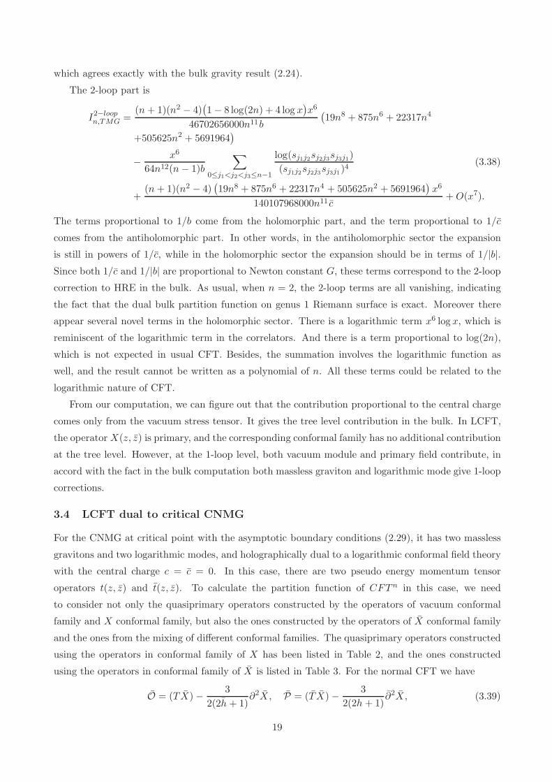
The 2-loop part is

I2−loopn,TMG =

(n+ 1)(n2 − 4)(

1− 8 log(2n) + 4 log x)

x6

46702656000n11b

(

19n8 + 875n6 + 22317n4

+505625n2 + 5691964)

− x6

64n12(n− 1)b

∑

0≤j1<j2<j3≤n−1

log(sj1j2sj2j3sj3j1)

(sj1j2sj2j3sj3j1)4

(3.38)

+(n+ 1)(n2 − 4)

(

19n8 + 875n6 + 22317n4 + 505625n2 + 5691964)

x6

140107968000n11 c+O(x7).

The terms proportional to 1/b come from the holomorphic part, and the term proportional to 1/c

comes from the antiholomorphic part. In other words, in the antiholomorphic sector the expansion

is still in powers of 1/c, while in the holomorphic sector the expansion should be in terms of 1/|b|.Since both 1/c and 1/|b| are proportional to Newton constant G, these terms correspond to the 2-loop

correction to HRE in the bulk. As usual, when n = 2, the 2-loop terms are all vanishing, indicating

the fact that the dual bulk partition function on genus 1 Riemann surface is exact. Moreover there

appear several novel terms in the holomorphic sector. There is a logarithmic term x6 log x, which is

reminiscent of the logarithmic term in the correlators. And there is a term proportional to log(2n),

which is not expected in usual CFT. Besides, the summation involves the logarithmic function as

well, and the result cannot be written as a polynomial of n. All these terms could be related to the

logarithmic nature of CFT.

From our computation, we can figure out that the contribution proportional to the central charge

comes only from the vacuum stress tensor. It gives the tree level contribution in the bulk. In LCFT,

the operator X(z, z) is primary, and the corresponding conformal family has no additional contribution

at the tree level. However, at the 1-loop level, both vacuum module and primary field contribute, in

accord with the fact in the bulk computation both massless graviton and logarithmic mode give 1-loop

corrections.

3.4 LCFT dual to critical CNMG

For the CNMG at critical point with the asymptotic boundary conditions (2.29), it has two massless

gravitons and two logarithmic modes, and holographically dual to a logarithmic conformal field theory

with the central charge c = c = 0. In this case, there are two pseudo energy momentum tensor

operators t(z, z) and t(z, z). To calculate the partition function of CFT n in this case, we need

to consider not only the quasiprimary operators constructed by the operators of vacuum conformal

family and X conformal family, but also the ones constructed by the operators of X conformal family

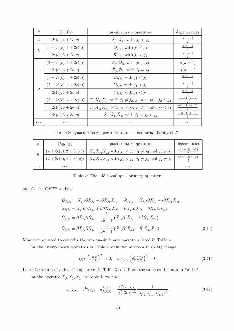
and the ones from the mixing of different conformal families. The quasiprimary operators constructed

using the operators in conformal family of X has been listed in Table 2, and the ones constructed

using the operators in conformal family of X is listed in Table 3. For the normal CFT we have

O = (TX)− 3

2(2h + 1)∂2X, P = (T X)− 3

2(2h + 1)∂2X, (3.39)

19

# (L0, L0) quasiprimary operators degeneracies

4 (2ǫ(c), 4 + 2ǫ(c)) Xj1Xj2 with j1 < j2n(n−1)

2

5(1 + 2ǫ(c), 4 + 2ǫ(c)) Qj1j2 with j1 < j2

n(n−1)2

(2ǫ(c), 5 + 2ǫ(c)) Rj1j2 with j1 < j2n(n−1)

2

6

(2 + 2ǫ(c), 4 + 2ǫ(c)) Xj1Oj2 with j1 6= j2 n(n− 1)

(2ǫ(c), 6 + 2ǫ(c)) Xj1Pj2 with j1 6= j2 n(n− 1)

(1 + 2ǫ(c), 5 + 2ǫ(c)) Sj1j2 with j1 < j2n(n−1)

2

(2 + 2ǫ(c), 4 + 2ǫ(c)) Uj1j2 with j1 < j2n(n−1)

2

(2ǫ(c), 6 + 2ǫ(c)) Vj1j2 with j1 < j2n(n−1)

2

(2 + 2ǫ(c), 4 + 2ǫ(c)) Tj1Xj2Xj3 with j1 6= j2, j1 6= j3 and j2 < j3n(n−1)(n−2)

2

(2ǫ(c), 6 + 2ǫ(c)) Tj1Xj2Xj3 with j1 6= j2, j1 6= j3 and j2 < j3n(n−1)(n−2)

2

(3ǫ(c), 6 + 3ǫ(c)) Xj1Xj2Xj3 with j1 < j2 < j3n(n−1)(n−2)

6

· · · · · · · · · · · ·

Table 3: Quasiprimary operators from the conformal family of X

# (L0, L0) quasiprimary operators degeneracies

6(4 + 3ǫ(c), 2 + 3ǫ(c)) Xj1Xj2Xj3 with j1 < j2, j1 6= j3 and j2 6= j3

n(n−1)(n−2)2

(2 + 3ǫ(c), 4 + 3ǫ(c)) Xj1Xj2Xj3 with j1 < j2, j1 6= j3 and j2 6= j3n(n−1)(n−2)

2

· · · · · · · · · · · ·

Table 4: The additional quasiprimary operators

and for the CFT n we have

Qj1j2 = Xj1i∂Xj2 − i∂Xj1Xj2 , Rj1j2 = Xj1i∂Xj2 − i∂Xj1Xj2 ,

Sj1j2 = Xj1∂∂Xj2 + ∂∂Xj1Xj2 − ∂Xj1 ∂Xj2 − ∂Xj1∂Xj2 ,

Uj1j2 = ∂Xj1∂Xj2 −h

2h+ 1

(

Xj1∂2Xj2 + ∂2Xj1Xj2

)

,

Vj1j2 = ∂Xj1 ∂Xj2 −h

2h+ 1

(

Xj1 ∂2Xj2 + ∂2Xj1Xj2

)

. (3.40)

Moreover we need to consider the two quasiprimary operators listed in Table 4.

For the quasiprimary operators in Table 2, only two relations in (3.34) change

αXP

(

dj1j2XP

)2→ 0, αTXX

(

dj1j2j3TXX

)2→ 0. (3.41)

It can be seen easily that the operators in Table 3 contribute the same as the ones in Table 2.

For the operator Xj1Xj2Xj3 in Table 4, we find

αXXX = i4sα3X , dj1j2j3

XXX=

i3sCXXX

α3X(2n)3∆

1

(sj1j2sj1j3sj2j3)∆, (3.42)

20

and when c → 0 we have

αXXX

(

dj1j2j3XXX

)2→ 0. (3.43)

Similarly when c → 0 we have

αXXX

(

dj1j2j3XXX

)2→ 0. (3.44)

So the operators in Table 4 do not contribute to the Renyi entropy.

Taking all the contributions into account, we can read the Renyi mutual information

INMGn = Itreen,NMG + I1−1oop

n,NMG + I2−loopn,NMG + · · · . (3.45)

The tree part is vanishing Itreen,NMG = 0, as we expected. The 1-loop part is

I1−loopn,NMG =

(n+ 1)(

n2 + 11) (

3n4 + 10n2 + 227)

x4

1814400n7

+(n+ 1)

(

109n8 + 1495n6 + 11307n4 + 81905n2 − 8416)

x5

29937600n9

+(n+ 1)x6

28740096000n11

(

158702n10 + 2100642n8 + 15450121n6 + 109973341n4

−18280323n2 − 538483)

+O(x7), (3.46)

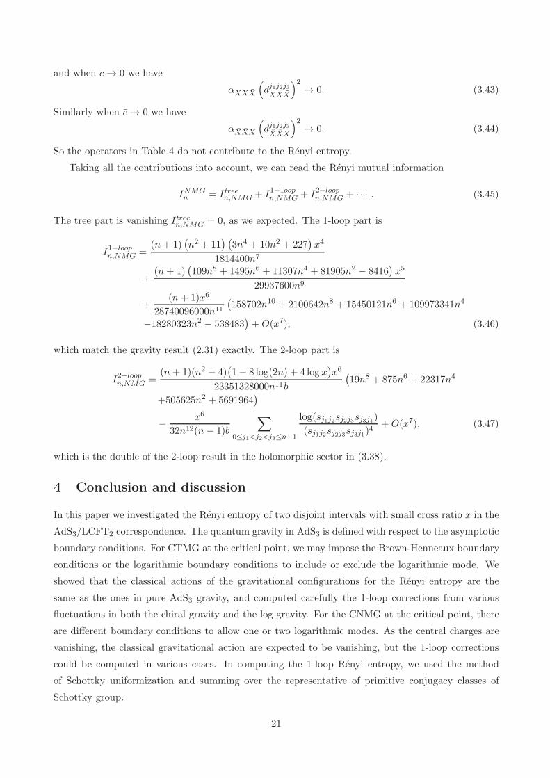
which match the gravity result (2.31) exactly. The 2-loop part is

I2−loopn,NMG =

(n+ 1)(n2 − 4)(

1− 8 log(2n) + 4 log x)

x6

23351328000n11b

(

19n8 + 875n6 + 22317n4

+505625n2 + 5691964)

− x6

32n12(n− 1)b

∑

0≤j1<j2<j3≤n−1

log(sj1j2sj2j3sj3j1)

(sj1j2sj2j3sj3j1)4

+O(x7), (3.47)

which is the double of the 2-loop result in the holomorphic sector in (3.38).

4 Conclusion and discussion

In this paper we investigated the Renyi entropy of two disjoint intervals with small cross ratio x in the

AdS3/LCFT2 correspondence. The quantum gravity in AdS3 is defined with respect to the asymptotic

boundary conditions. For CTMG at the critical point, we may impose the Brown-Henneaux boundary

conditions or the logarithmic boundary conditions to include or exclude the logarithmic mode. We

showed that the classical actions of the gravitational configurations for the Renyi entropy are the

same as the ones in pure AdS3 gravity, and computed carefully the 1-loop corrections from various

fluctuations in both the chiral gravity and the log gravity. For the CNMG at the critical point, there

are different boundary conditions to allow one or two logarithmic modes. As the central charges are

vanishing, the classical gravitational action are expected to be vanishing, but the 1-loop corrections

could be computed in various cases. In computing the 1-loop Renyi entropy, we used the method

of Schottky uniformization and summing over the representative of primitive conjugacy classes of

Schottky group.

21

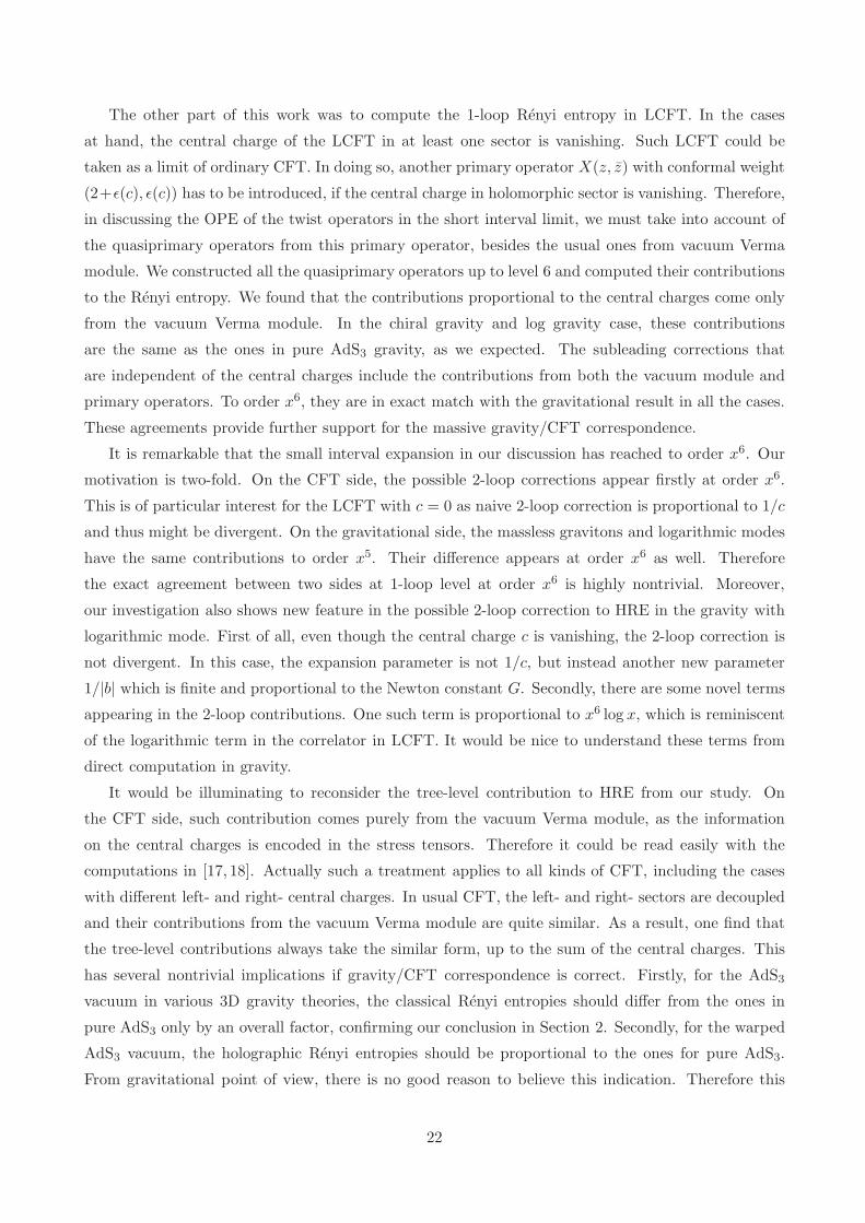
The other part of this work was to compute the 1-loop Renyi entropy in LCFT. In the cases

at hand, the central charge of the LCFT in at least one sector is vanishing. Such LCFT could be

taken as a limit of ordinary CFT. In doing so, another primary operator X(z, z) with conformal weight

(2+ǫ(c), ǫ(c)) has to be introduced, if the central charge in holomorphic sector is vanishing. Therefore,

in discussing the OPE of the twist operators in the short interval limit, we must take into account of

the quasiprimary operators from this primary operator, besides the usual ones from vacuum Verma

module. We constructed all the quasiprimary operators up to level 6 and computed their contributions

to the Renyi entropy. We found that the contributions proportional to the central charges come only

from the vacuum Verma module. In the chiral gravity and log gravity case, these contributions

are the same as the ones in pure AdS3 gravity, as we expected. The subleading corrections that

are independent of the central charges include the contributions from both the vacuum module and

primary operators. To order x6, they are in exact match with the gravitational result in all the cases.

These agreements provide further support for the massive gravity/CFT correspondence.

It is remarkable that the small interval expansion in our discussion has reached to order x6. Our

motivation is two-fold. On the CFT side, the possible 2-loop corrections appear firstly at order x6.

This is of particular interest for the LCFT with c = 0 as naive 2-loop correction is proportional to 1/c

and thus might be divergent. On the gravitational side, the massless gravitons and logarithmic modes

have the same contributions to order x5. Their difference appears at order x6 as well. Therefore

the exact agreement between two sides at 1-loop level at order x6 is highly nontrivial. Moreover,

our investigation also shows new feature in the possible 2-loop correction to HRE in the gravity with

logarithmic mode. First of all, even though the central charge c is vanishing, the 2-loop correction is

not divergent. In this case, the expansion parameter is not 1/c, but instead another new parameter

1/|b| which is finite and proportional to the Newton constant G. Secondly, there are some novel terms

appearing in the 2-loop contributions. One such term is proportional to x6 log x, which is reminiscent

of the logarithmic term in the correlator in LCFT. It would be nice to understand these terms from

direct computation in gravity.

It would be illuminating to reconsider the tree-level contribution to HRE from our study. On

the CFT side, such contribution comes purely from the vacuum Verma module, as the information

on the central charges is encoded in the stress tensors. Therefore it could be read easily with the

computations in [17, 18]. Actually such a treatment applies to all kinds of CFT, including the cases

with different left- and right- central charges. In usual CFT, the left- and right- sectors are decoupled

and their contributions from the vacuum Verma module are quite similar. As a result, one find that

the tree-level contributions always take the similar form, up to the sum of the central charges. This

has several nontrivial implications if gravity/CFT correspondence is correct. Firstly, for the AdS3

vacuum in various 3D gravity theories, the classical Renyi entropies should differ from the ones in

pure AdS3 only by an overall factor, confirming our conclusion in Section 2. Secondly, for the warped

AdS3 vacuum, the holographic Renyi entropies should be proportional to the ones for pure AdS3.

From gravitational point of view, there is no good reason to believe this indication. Therefore this

22

raises a serious challenge to the warped AdS3/CFT2 correspondence.

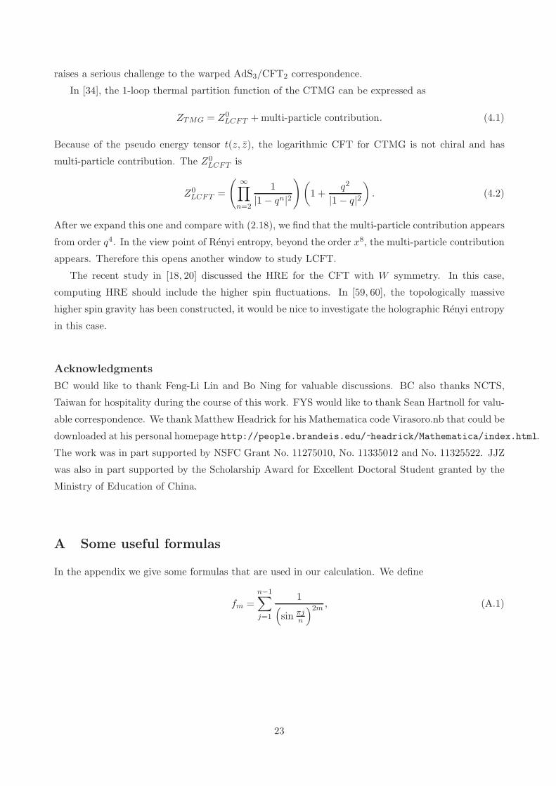
In [34], the 1-loop thermal partition function of the CTMG can be expressed as

ZTMG = Z0LCFT +multi-particle contribution. (4.1)

Because of the pseudo energy tensor t(z, z), the logarithmic CFT for CTMG is not chiral and has

multi-particle contribution. The Z0LCFT is

Z0LCFT =

(

∞∏

n=2

1

|1− qn|2

)

(

1 +q2

|1− q|2)

. (4.2)

After we expand this one and compare with (2.18), we find that the multi-particle contribution appears

from order q4. In the view point of Renyi entropy, beyond the order x8, the multi-particle contribution

appears. Therefore this opens another window to study LCFT.

The recent study in [18, 20] discussed the HRE for the CFT with W symmetry. In this case,

computing HRE should include the higher spin fluctuations. In [59, 60], the topologically massive

higher spin gravity has been constructed, it would be nice to investigate the holographic Renyi entropy

in this case.

Acknowledgments

BC would like to thank Feng-Li Lin and Bo Ning for valuable discussions. BC also thanks NCTS,

Taiwan for hospitality during the course of this work. FYS would like to thank Sean Hartnoll for valu-

able correspondence. We thank Matthew Headrick for his Mathematica code Virasoro.nb that could be

downloaded at his personal homepage http://people.brandeis.edu/~headrick/Mathematica/index.html.

The work was in part supported by NSFC Grant No. 11275010, No. 11335012 and No. 11325522. JJZ

was also in part supported by the Scholarship Award for Excellent Doctoral Student granted by the

Ministry of Education of China.

A Some useful formulas

In the appendix we give some formulas that are used in our calculation. We define

fm =

n−1∑

j=1

1(

sin πjn

)2m , (A.1)

23

and explicitly we need

f1 =n2 − 1

3, f2 =

(n2 − 1)(

n2 + 11)

45, f3 =

(n2 − 1)(

2n4 + 23n2 + 191)

945,

f4 =(n2 − 1)

(

n2 + 11) (

3n4 + 10n2 + 227)

14175,

f5 =(n2 − 1)

(

2n8 + 35n6 + 321n4 + 2125n2 + 14797)

93555, (A.2)

f6 =(n2 − 1)

(

1382n10 + 28682n8 + 307961n6 + 2295661n4 + 13803157n2 + 92427157)

638512875.

The above formulas are useful because they often appear in the following summations

∑

0≤j1<j2≤n−1

1

s2mj1j2=

n

2fm, (A.3)

∑

0≤j1<j2<j3≤n−1

(

1

s2mj1j2+

1

s2mj2j3+

1

s2mj3j1

)

=n(n− 2)

2fm.

There are also several other useful summation formulas

∑

0≤j1<j2<j3≤n−1

1

s2j1j2s2j2j3

s2j3j1=

n(

n2 − 1) (

n2 − 4) (

n2 + 47)

2835,

∑

0≤j1<j2<j3≤n−1

1

s4j1j2s4j2j3

s4j3j1=

n(

n2 − 1) (

n2 − 4)

273648375

(

19n8 + 875n6 + 22317n4

+505625n2 + 5691964)

, (A.4)

∑

0≤j1<j2<j3≤n−1

1

s2j1j2s2j2j3

s2j3j1

(

1

s4j1j2+

1

s4j2j3+

1

s4j3j1

)

=n(n2 − 1)(n2 − 4)

467775

(

3n6 + 125n4

+1757n2 + 21155)

,

∑

0≤j1<j2<j3≤n−1

(

1

s4j1j2s4j2j3

+1

s4j2j3s4j3j1

+1

s4j3j1s4j1j2

)

=2n(n2 − 1)(n2 − 4)

(

n2 + 11) (

n2 + 19)

14175.

References

[1] L. Bombelli, R. K. Koul, J. Lee, and R. D. Sorkin, “A Quantum Source of Entropy for Black

Holes,” Phys.Rev. D34 (1986) 373–383.

[2] M. Srednicki, “Entropy and area,” Phys.Rev.Lett. 71 (1993) 666–669,

arXiv:hep-th/9303048 [hep-th].

[3] J. Callan, Curtis G. and F. Wilczek, “On geometric entropy,” Phys.Lett. B333 (1994) 55–61,

arXiv:hep-th/9401072 [hep-th].

[4] S. Ryu and T. Takayanagi, “Holographic derivation of entanglement entropy from AdS/CFT,”

Phys.Rev.Lett. 96 (2006) 181602, arXiv:hep-th/0603001 [hep-th].

24

[5] S. Ryu and T. Takayanagi, “Aspects of Holographic Entanglement Entropy,”

JHEP 0608 (2006) 045, arXiv:hep-th/0605073 [hep-th].

[6] T. Nishioka, S. Ryu, and T. Takayanagi, “Holographic Entanglement Entropy: An Overview,”

J.Phys. A42 (2009) 504008, arXiv:0905.0932 [hep-th].

[7] T. Takayanagi, “Entanglement Entropy from a Holographic Viewpoint,”

Class.Quant.Grav. 29 (2012) 153001, arXiv:1204.2450 [gr-qc].

[8] M. Headrick, “Entanglement Renyi entropies in holographic theories,”

Phys.Rev. D82 (2010) 126010, arXiv:1006.0047 [hep-th].

[9] L.-Y. Hung, R. C. Myers, M. Smolkin, and A. Yale, “Holographic Calculations of Renyi

Entropy,” JHEP 1112 (2011) 047, arXiv:1110.1084 [hep-th].

[10] T. Hartman, “Entanglement Entropy at Large Central Charge,” arXiv:1303.6955 [hep-th].

[11] T. Faulkner, “The Entanglement Renyi Entropies of Disjoint Intervals in AdS/CFT,”

arXiv:1303.7221 [hep-th].

[12] A. Lewkowycz and J. Maldacena, “Generalized gravitational entropy,” JHEP 1308 (2013) 090,

arXiv:1304.4926 [hep-th].

[13] D. V. Fursaev, “Proof of the holographic formula for entanglement entropy,”

JHEP 0609 (2006) 018, arXiv:hep-th/0606184 [hep-th].

[14] H. Casini, M. Huerta, and R. C. Myers, “Towards a derivation of holographic entanglement

entropy,” JHEP 1105 (2011) 036, arXiv:1102.0440 [hep-th].

[15] T. Barrella, X. Dong, S. A. Hartnoll, and V. L. Martin, “Holographic entanglement beyond

classical gravity,” arXiv:1306.4682 [hep-th].

[16] T. Faulkner, A. Lewkowycz, and J. Maldacena, “Quantum corrections to holographic

entanglement entropy,” arXiv:1307.2892 [hep-th].

[17] B. Chen and J.-J. Zhang, “On short interval expansion of Rnyi entropy,”

JHEP 1311 (2013) 164, arXiv:1309.5453 [hep-th].

[18] B. Chen, J. Long, and J.-j. Zhang, “Holographic Renyi entropy for CFT with W symmetry,”

arXiv:1312.5510 [hep-th].

[19] P. Calabrese, J. Cardy, and E. Tonni, “Entanglement entropy of two disjoint intervals in

conformal field theory II,” J.Stat.Mech. 1101 (2011) P01021, arXiv:1011.5482 [hep-th].

[20] E. Perlmutter, “Comments on Renyi entropy in AdS3/CFT2,” arXiv:1312.5740 [hep-th].

25

[21] S. Deser, R. Jackiw, and S. Templeton, “Topologically Massive Gauge Theories,”

Annals Phys. 140 (1982) 372–411.

[22] S. Deser, R. Jackiw, and S. Templeton, “Three-Dimensional Massive Gauge Theories,”

Phys.Rev.Lett. 48 (1982) 975–978.

[23] E. A. Bergshoeff, O. Hohm, and P. K. Townsend, “Massive Gravity in Three Dimensions,”

Phys.Rev.Lett. 102 (2009) 201301, arXiv:0901.1766 [hep-th].

[24] E. A. Bergshoeff, O. Hohm, and P. K. Townsend, “More on Massive 3D Gravity,”

Phys.Rev. D79 (2009) 124042, arXiv:0905.1259 [hep-th].

[25] W. Li, W. Song, and A. Strominger, “Chiral Gravity in Three Dimensions,”

JHEP 0804 (2008) 082, arXiv:0801.4566 [hep-th].

[26] A. Strominger, “A Simple Proof of the Chiral Gravity Conjecture,”

arXiv:0808.0506 [hep-th].

[27] S. Carlip, S. Deser, A. Waldron, and D. Wise, “Cosmological Topologically Massive Gravitons

and Photons,” Class.Quant.Grav. 26 (2009) 075008, arXiv:0803.3998 [hep-th].

[28] S. Carlip, S. Deser, A. Waldron, and D. Wise, “Topologically Massive AdS Gravity,”

Phys.Lett. B666 (2008) 272–276, arXiv:0807.0486 [hep-th].

[29] D. Grumiller and N. Johansson, “Instability in cosmological topologically massive gravity at the

chiral point,” JHEP 0807 (2008) 134, arXiv:0805.2610 [hep-th].

[30] D. Grumiller and N. Johansson, “Consistent boundary conditions for cosmological topologically

massive gravity at the chiral point,” Int.J.Mod.Phys. D17 (2009) 2367–2372,

arXiv:0808.2575 [hep-th].

[31] M. Henneaux, C. Martinez, and R. Troncoso, “Asymptotically anti-de Sitter spacetimes in

topologically massive gravity,” Phys.Rev. D79 (2009) 081502, arXiv:0901.2874 [hep-th].

[32] A. Maloney, W. Song, and A. Strominger, “Chiral Gravity, Log Gravity and Extremal CFT,”

Phys.Rev. D81 (2010) 064007, arXiv:0903.4573 [hep-th].

[33] D. Grumiller and I. Sachs, “AdS (3) / LCFT (2) — Correlators in Cosmological Topologically

Massive Gravity,” JHEP 1003 (2010) 012, arXiv:0910.5241 [hep-th].

[34] M. R. Gaberdiel, D. Grumiller, and D. Vassilevich, “Graviton 1-loop partition function for

3-dimensional massive gravity,” JHEP 1011 (2010) 094, arXiv:1007.5189 [hep-th].

[35] Y. Liu and Y.-w. Sun, “Note on New Massive Gravity in AdS(3),” JHEP 0904 (2009) 106,

arXiv:0903.0536 [hep-th].

26

[36] Y. Liu and Y.-W. Sun, “Consistent Boundary Conditions for New Massive Gravity in AdS3,”

JHEP 0905 (2009) 039, arXiv:0903.2933 [hep-th].

[37] D. Grumiller and O. Hohm, “AdS(3)/LCFT(2): Correlators in New Massive Gravity,”

Phys.Lett. B686 (2010) 264–267, arXiv:0911.4274 [hep-th].

[38] K. Krasnov, “Holography and Riemann surfaces,” Adv.Theor.Math.Phys. 4 (2000) 929–979,

arXiv:hep-th/0005106 [hep-th].

[39] P. Kraus and F. Larsen, “Microscopic black hole entropy in theories with higher derivatives,”

JHEP 0509 (2005) 034, arXiv:hep-th/0506176 [hep-th].

[40] P. G. Zograf and L. A. Takhtadzhyan, “On uniformization of riemann surfaces and the

weil-petersson metric on teichmller and schottky spaces,” Mathematics of the USSR-Sbornik 60

(1988) 297. http://iopscience.iop.org/0025-5734/60/2/A03.

[41] P. Kraus and F. Larsen, “Holographic gravitational anomalies,” JHEP 0601 (2006) 022,

arXiv:hep-th/0508218 [hep-th].

[42] S. N. Solodukhin, “Holography with gravitational Chern-Simons,”

Phys.Rev. D74 (2006) 024015, arXiv:hep-th/0509148 [hep-th].

[43] J. D. Brown and M. Henneaux, “Central Charges in the Canonical Realization of Asymptotic

Symmetries: An Example from Three-Dimensional Gravity,”

Commun.Math.Phys. 104 (1986) 207–226.

[44] S. Giombi, A. Maloney, and X. Yin, “One-loop Partition Functions of 3D Gravity,”

JHEP 0808 (2008) 007, arXiv:0804.1773 [hep-th].

[45] J. R. David, M. R. Gaberdiel, and R. Gopakumar, “The Heat Kernel on AdS(3) and its

Applications,” JHEP 1004 (2010) 125, arXiv:0911.5085 [hep-th].

[46] A. Bhattacharyya, M. Sharma, and A. Sinha, “On generalized gravitational entropy, squashed

cones and holography,” arXiv:1308.5748 [hep-th].

[47] V. Gurarie, “Logarithmic operators in conformal field theory,”

Nucl.Phys. B410 (1993) 535–549, arXiv:hep-th/9303160 [hep-th].

[48] I. I. Kogan and A. Nichols, “Stress energy tensor in LCFT and the logarithmic Sugawara

construction,” JHEP 0201 (2002) 029, arXiv:hep-th/0112008 [hep-th].

[49] I. I. Kogan and A. Nichols, “Stress energy tensor in C = 0 logarithmic conformal field theory,”

arXiv:hep-th/0203207 [hep-th].

27

[50] S. Moghimi-Araghi, S. Rouhani, and M. Saadat, “Logarithmic conformal field theory through

nilpotent conformal dimensions,” Nucl.Phys. B599 (2001) 531–546,

arXiv:hep-th/0008165 [hep-th].

[51] M. A. Flohr, “Singular vectors in logarithmic conformal field theories,”

Nucl.Phys. B514 (1998) 523–552, arXiv:hep-th/9707090 [hep-th].

[52] J. Cardy, “Logarithmic Correlations in Quenched Random Magnets and Polymers,”

arXiv:cond-mat/9911024 [cond-mat].

[53] V. Gurarie and A. W. W. Ludwig, “LETTER TO THE EDITOR: Conformal algebras of

two-dimensional disordered systems,” J. Phys. A: Math. Theor. 35 (2002) 377,

arXiv:cond-mat/9911392 [cond-mat].

[54] J. Cardy, “The Stress Tensor in Quenched Random Systems,”

arXiv:cond-mat/0111031 [cond-mat].

[55] D. Grumiller, W. Riedler, J. Rosseel, and T. Zojer, “Holographic applications of logarithmic

conformal field theories,” J. Phys. A: Math. Theor. 46 (2013) 494002,

arXiv:1302.0280 [hep-th].

[56] J. Cardy, “Logarithmic conformal field theories as limits of ordinary CFTs and some physical

applications,” J.Phys. A46 (2013) 494001, arXiv:1302.4279 [cond-mat.stat-mech].

[57] P. Calabrese and J. L. Cardy, “Entanglement entropy and quantum field theory,”

J.Stat.Mech. 0406 (2004) P06002, arXiv:hep-th/0405152 [hep-th].

[58] P. Calabrese and J. Cardy, “Entanglement entropy and conformal field theory,”

J.Phys. A42 (2009) 504005, arXiv:0905.4013 [cond-mat.stat-mech].

[59] B. Chen, J. Long, and J.-B. Wu, “Spin-3 Topological Massive Gravity,”

Phys.Lett. B705 (2011) 513–520, arXiv:1106.5141 [hep-th].

[60] B. Chen and J. Long, “High Spin Topologically Massive Gravity,” JHEP 1112 (2011) 114,

arXiv:1110.5113 [hep-th].

28