Homeomorphisms of the Mandelbrot Set

Wolf Jung

Abstract

On subsets of the Mandelbrot set, EM ⊂M, homeomorphisms are constructedby quasi-conformal surgery. When the dynamics of quadratic polynomials ischanged piecewise by a combinatorial construction, a general theorem yieldsthe corresponding homeomorphism h : EM → EM in the parameter plane.Each h has two fixed points in EM , and a countable family of mutually ho-meomorphic fundamental domains. Possible generalizations to other familiesof polynomials or rational mappings are discussed.The homeomorphisms on subsets EM ⊂ M constructed by surgery are ex-tended to homeomorphisms of M, and employed to study groups of non-trivial homeomorphisms h : M→M. It is shown that these groups have thecardinality of R, and they are not compact.

Preprint of a paper submitted to Dynamics in the Complex Plane, proceedings of a sym-posium in honour of Bodil Branner, June 19–21 2003, Holbæk.

1 Introduction

Consider the family of complex quadratic polynomials fc(z) := z2 + c. They are

parametrized by c ∈ C, which is at the same time the critical value of fc , since 0 is

the critical point. The filled Julia set Kc of fc is a compact subset of the dynamic

plane. It contains all z ∈ C which are not attracted to ∞ under the iteration of fc ,

i.e. fnc (z) 6→ ∞. The global dynamics is determined qualitatively by the behavior

of the critical point or critical value under iteration. E.g., by a classical theorem of

Fatou, Kc is connected iff fnc (c) 6→ ∞, i.e. c ∈ Kc . The Mandelbrot setM is a subset

of the parameter plane, it contains precisely the parameters with this property.

Although it can be defined by the recursive computation of the critical orbit, with

no reference to the whole dynamic plane, most results on M are obtained by an

interplay between both planes: starting with a subset EM ⊂M, employ the dynamics

of fc to find a common structure in Kc for all c ∈ EM . Then an analogous structure

will be found in EM , i.e. in the parameter plane. This principle has various precise

formulations. Most important is its application to external rays: these are curves

in the complement of Kc (dynamic rays) or in the complement of M (parameter

rays), which are labeled by an angle θ ∈ S1 = R/Z. For rational angles θ ∈ Q/Z,

1

these rays are landing at special points in ∂Kc or ∂M, respectively. See Sect. 2.1 for

details. When rays are landing together, the landing point is called a pinching point.

It can be used to disconnect Kc or M into well-defined components. The structure

of Kc , as described by these pinching points, can be understood dynamically, and

then these results are transfered to the parameter plane, to understand the structure

of M.

?6

⇒

⇐

ψcψd

fc gc

fdgd

Figure 1: A simulation of Branner–Douady surgery ΦA : M1/2 → T ⊂ M1/3 , as ex-plained in the text below. In this simulation, gc and gd are defined piecewise explicitly,and the required Riemann mappings are replaced with simple affine mappings.

Each filled Julia set Kc is completely invariant under the corresponding mapping fc ,

and this fact explains the self-similarity of these sets. On the other hand, when the

parameter cmoves through the Mandelbrot set, the corresponding Julia sets undergo

an infinite number of bifurcations. By the above principle, the local structure of Mis undergoing corresponding changes as well. But these changes may combine in

such a way, that subsets of M are mutually homeomorphic. Such homeomorphisms

can be constructed by quasi-conformal surgery. There are three basic ideas (the first

and second apply to more general situations [5]):

• A mapping g with desired dynamics is constructed piecewise, i.e. by piecing

together different mappings or different iterates of one mapping. The pieces

are defined e.g. by dynamic rays landing at pinching points of the Julia set.

• g cannot be analytic, but one constructs a quasi-conformal mapping ψ such

that the composition f = ψgψ−1 is analytic. This is possible, when a field of

infinitesimal ellipses is found that is invariant under g. Then ψ is constructed

such that it is mapping these ellipses to infinitesimal circles. (See Sect. 2.2 for

the precise definition of quasi-conformal mappings.)

2

• Suppose that fc is a one-parameter family of analytic mappings, e.g. our

quadratic polynomials, and that gc is constructed piecewise from iterates of fc

for parameters c ∈ EM ⊂ M. If ψc gc ψ−1c = fd , a mapping in parameter

space is obtained from h(c) := d. There are techniques to show that h is a

homeomorphism.

Homeomorphisms of the Mandelbrot set have been obtained in [6, 1, 2, 3, 13, 8]. We

shall discuss the example of the Branner–Douady homeomorphism ΦA , cf. Fig. 1:

parameters c in the limb M1/2 of M are characterized by the fact, that the Julia set

Kc has two branches at the fixed point αc and at its countable family of preimages.

By a piecewise construction, fc is replaced with a new mapping gc , such that a

third branch appears at αc , and thus at its preimages as well. This can be done by

cut- and paste techniques on a Riemann surface, or by conformal mappings between

sectors in the dynamic plane. Since gc is analytic except in some smaller sectors, it

is possible to construct an invariant ellipse field. The corresponding quasi-conformal

mapping ψc is used to conjugate gc to a (unique) quadratic polynomial fd , and the

mapping in parameter space is defined by ΦA(c) := d. Now the Julia sets of fd and

gc are homeomorphic, and the dynamics are conjugate. The parameter d belongs

to the limb M1/3 , since the three branches of Kd at αd are permuted by fd with

rotation number 1/3. Now there is an analogous construction of a mapping gd for

d ∈ T ⊂ M1/3 , which turns out to yield the inverse mapping ΦA. The Julia set

of gd has lost some arms, and gd is conjugate to a quadratic polynomial fe again.

By showing that fc and fe are conjugate, it follows that e = c, thus ΦA ΦA = id.

(The uniqueness follows from the fact that these quasi-conformal conjugations are

hybrid-equivalences, i.e. conformal almost everywhere on the filled Julia sets [6].)

For the homeomorphisms constructed in this paper, the mapping gc is defined piece-

wise by compositions of iterates of fc , and no cut- and paste techniques or conformal

mappings are used. Then the Julia sets of fc and gc are the same, and no arms are

lost or added in the parameter plane either: a subset EM ⊂ M is defined by dis-

connecting M at two pinching points, and this subset is mapped onto itself by the

homeomorphism (which is not the identity, of course). Thus a countable family of

mutually homeomorphic subsets is obtained from one construction. General com-

binatorial assumptions are presented in Sect. 3.1, which allow the definition of a

preliminary mapping g(1)c analogous to the example in Fig. 2: it differs from fc on

two strips Vc , Wc , where it is of the form f−nc (±fm

c ). Basically, we only need to

find four strips with Vc ∪Wc = Vc ∪ Wc , such that these are mapped as Vc → Vc ,

Wc → Wc by suitable compositions of ±f±1c .

Theorem 1.1 (Construction and Properties of h)

1. Given the combinatorial construction of EM ⊂M and g(1)c for c ∈ EM according to

Def. 3.1, there is a family of “quasi-quadratic” mappings gc coinciding with g(1)c on

the filled Julia sets Kc . These are hybrid-equivalent to unique quadratic polynomials.

2. The mapping h : EM → EM in parameter space is defined as follows: for c ∈ EM ,

3

find the polynomial fd that is hybrid-equivalent to gc , and set h(c) := d. It does not

depend on the precise choice of gc (only on the combinatorial definition of g(1)c ). Now

h is a homeomorphism, and analytic in the interior of EM .

3. h is a non-trivial homeomorphism of EM onto itself, fixing the vertices a and b.

h and h−1 are Holder continuous at Misiurewicz points and Lipschitz continuous

at a and b. Moreover, h is expanding at a and contracting at b, cf. Fig. 3: for

c ∈ EM \a, b we have hn(c) → b as n→∞, and h−n(c) → a. There is a countable

family of mutually homeomorphic fundamental domains.

4. h extends to a homeomorphism between strips, h : PM → PM , which is quasi-

conformal in the exterior of M.

The power of Thm. 1.1 lies in turning combinatorial data into homeomorphisms. The

creative step remaining is to find eight angles Θ±i , such that there are compositions

of ±f±1c mapping Vc → Vc and Wc → Wc . When this is done, the existence of a

corresponding homeomorphisms is guaranteed by the theorem.

Θ−1Θ−

2Θ−3

Θ−4Θ+

4

Θ+3

Θ+2

Θ+1

Θ−1

Θ−2

Θ−4Θ+

4

Θ+2

Θ+1

Θ−1

Θ−3

Θ−4Θ+

4

Θ+3

Θ+1

Vc

Wc

Vc

Wc

Figure 2: Left: a parameter edge EM ⊂ M and the strip PM . Middle and right: thedynamic edge Ec ⊂ Kc in the strip Vc ∪Wc = Vc ∪ Wc . According to Sect. 3.1, these stripsare bounded by external rays, which belong to eight angles Θ±

i . In this example, we haveΘ−

1 = 11/56, Θ−2 = 199/1008, Θ−

3 = 103/504, Θ−4 = 23/112, Θ+

4 = 29/112, Θ+3 = 131/504,

Θ+2 = 269/1008, and Θ+

1 = 15/56. The first-return numbers are kw = kv = 4, kv = kw = 7.Now gc = g(1)

c on Kc and g(1)c = fc ηc , with ηc = f−2

c (−f5c ) = f−3

c (+f6c ) : Vc → Vc ,

ηc = f−6c (−f3

c ) : Wc → Wc . See also Fig. 3.

In Sections 2 and 3, basic properties of M and of quasi-conformal mappings are

recalled, and the proof of Thm. 1.1 is sketched by constructing gc and h. Re-

lated results from the author’s thesis [8] are summarized in Sect. 4. These include

more examples of homeomorphisms, constructed at chosen Misiurewicz points or

on “edges,” and the combinatorial description of homeomorphisms. When a one-

parameter family of polynomials is defined by critical relations, homeomorphisms in

parameter space can be obtained by analogous techniques. The same applies e.g. to

the rational mappings arising in Newton’s method for cubic polynomials.

H. Kriete has suggested that the homeomorphisms h : EM → EM constructed by this

kind of surgery extend to homeomorphisms of M. Thus they can be used to study

4

the homeomorphism group of M, answering a question by K. Keller. In Sect. 5,

some possible definitions for groups of non-trivial homeomorphisms are discussed,

and some properties are obtained by combining two tools: the characterization of

homeomorphisms by permutations of hyperbolic components, and the composition

of homeomorphisms constructed by surgery. The groups are not compact, and the

groups of non-trivial homeomorphisms have the cardinality of R.

a

b

c′7

c4

c′′7

JJ

JJJ]

JJ

JJJ]

h

h

Kc′7

Kc4

Kc′′7

JJ

JJ

JJ]

JJ

JJ

JJ]

ψc′7

ψc4

Figure 3: Left: the parameter edge EM from a := γM(11/56) to b := γM(23/112), thesame as in Fig. 2. The homeomorphism h : EM → EM is expanding at a and contracting atb. The centers of periods 4 and 7 are mapped as h : c′7 7→ c4 7→ c′′7 . Right: the filled Juliasets for c′7 , c4 , and c′′7 are quasi-conformally homeomorphic. (Ec ⊂ Kc is barely visible inthe top right corner.)

Acknowledgment

Many people have contributed to this work by inspiring discussions and helpful

suggestions. I wish to thank in particular Mohamed Barakat, Walter Bergweiler,

Volker Enss, Nuria Fagella, John Hamal Hubbard, Gerhard Jank, Karsten Keller,

Hartje Kriete, Fernando Lledo, Olaf Post, Johannes Riedl, and Dierk Schleicher.

I am especially happy to contribute this paper to the proceedings of a conference in

honor of Bodil Branner, since I have learned surgery from her papers [1, 2].

5

2 Background

Our main tools are the landing properties of external rays, and sending an ellipse

field to circles by a quasi-conformal mapping.

2.1 The Mandelbrot Set

fc(z) = z2 + c has a superattracting fixed point at ∞ ∈ C := C ∪ ∞. The

unique Boettcher conjugation is conjugating fc to F (z) := z2, Φc fc = F Φc in a

neighborhood of ∞. If the critical point 0, or the critical value c, does not escape

to ∞, then Kc is connected [5], and the parameter c belongs to the Mandelbrot set

M by definition. Then Φc extends to a conformal mapping Φc : C \ Kc → C \ D,

where D is the closed unit disk. Dynamic rays Rc(θ) are defined as preimages of

straight rays R(θ) = z | 1 < |z| < ∞, arg(z) = 2πθ under Φc . Theses curves in

the complement of Kc may land at a point in ∂Kc , or accumulate at the boundary

without landing. But they are always landing when θ is rational. Each rational angle

θ is periodic or preperiodic under doubling (mod 1). In the former case, the dynamic

ray Rc(θ) is landing at a periodic point z = γc(θ) ∈ ∂Kc , and at a preperiodic point

in the latter case. These properties are understood from fc(Rc(θ)) = Rc(2θ), since

arg(F (z)) = 2 arg(z).

The Mandelbrot set is compact, connected, and full, and the conformal mapping

ΦM : C \ M → C \ D is given by ΦM(c) := Φc(c). (When c /∈ M, Kc is totally

disconnected and Φc is not defined in all of its complement, but it is well-defined

at the critical value.) Parameter rays RM(θ) are defined as preimages of straight

rays under ΦM . Their landing properties are obtained e.g. in [16]: each rational

ray RM(θ) is landing at a point c = γM(θ) ∈ ∂M. When θ is preperiodic, then the

critical value c of fc is preperiodic, and the parameter c is called a Misiurewicz point.

The critical value c ∈ Kc has the same external angles as the parameter c ∈ M.

When θ is periodic, then c is the root of a hyperbolic component (see below). Both

in the dynamic plane of fc and in the parameter plane, the landing points of two

or more rational rays are called pinching points. They are used to disconnect these

sets into well-defined components, which are described combinatorially by rational

numbers. Their structure is obtained from the dynamics, and transfered to the

parameter plane. Pinching points with more than two branches are branch points.

Hyperbolic components of M consist of parameters, such that the corresponding

polynomial has an attracting cycle. The root is the parameter on the boundary,

such that the cycle has multiplier 1. The boundary of a hyperbolic component

contains a dense set of roots of satellite components. Each hyperbolic component

has a unique center, where the corresponding cycle is superattracting. Centers or

roots are dense at/in ∂M.

6

2.2 Quasi-Conformal Mappings

An orientation-preserving homeomorphism ψ between domains in C is K-quasi-

conformal, 1 ≤ K <∞, if it has two properties:

• It is weakly differentiable, so that its differential dψ = ∂ψ dz+∂ψ dz is defined

almost everywhere. This linear map is sending certain ellipses in the tangent

space to circles. The Beltrami coefficient µ := ∂ψ/∂ψ is defined almost every-

where. It encodes the direction and the dilatation ratio of the semi-axes for

the ellipse field [5].

• The dilatation ratio is bounded globally by K, or |µ(z)| ≤ (K − 1)/(K + 1)

almost everywhere.

The chain rule for derivatives is satisfied for the composition of quasi-conformal map-

pings, and a 1-quasi-conformal mapping is conformal. Quasi-conformal mappings

are absolutely continuous, Holder continuous, and have nice properties regarding

e.g. boundary behavior or normal families [10]. Given a measurable ellipse field

(Beltrami coefficient) µ with |µ(z)| ≤ m < 1 almost everywhere, the Beltrami dif-

ferential equation ∂ψ = µ∂ψ on C has a unique solution with the normalization

ψ(z) = z + o(1) as z → ∞. The dependence on parameters is described by the

Ahlfors–Bers Theorem [5], which is behind some of our arguments, but will not be

used explicitly here.

A K-quasi-regular mapping is locally K-quasi-conformal except for critical points,

but it need not be injective globally. In Sect. 3.3, we will have a quasi-regular

mapping g, such that all iterates areK-quasi-regular, and analytic in a neighborhood

of ∞. Then a g-invariant field of infinitesimal ellipses is obtained as follows: it

consists of circles in a neighborhood of ∞, i.e. µ(z) = 0 there, and it is pulled back

with iterates of g. Now ψ shall solve the corresponding Beltrami equation, i.e. send

these ellipses to circles. By the chain rule, f := ψ g ψ−1 is mapping almost every

infinitesimal circle to a circle, thus it is analytic.

3 Quasi-Conformal Surgery

As soon as the combinatorial assumptions on g(1)c given here are satisfied, Thm. 1.1

yields a corresponding homeomorphism of EM . After formulating these general

assumptions, the proof is sketched by constructing the quasi-quadratic mapping gc

and the homeomorphism h. For some details, the reader will be referred to [8].

3.1 Combinatorial Setting

The following definitions may be illustrated by the example in Fig. 2. Further

examples are mentioned in Sects. 4.2–4.4. When four parameter rays are landing

7

in pairs at two pinching points of M, this defines a strip in the parameter plane.

Analogously, four dynamic rays define a strip in the dynamic plane. Our assumptions

are formulated in terms of eight preperiodic angles

0 < Θ−1 < Θ−

2 < Θ−3 < Θ−

4 < Θ+4 < Θ+

3 < Θ+2 < Θ+

1 < 1 . (1)

• The Misiurewicz points a := γM(Θ−1 ) = γM(Θ+

1 ) 6= γM(Θ−4 ) = γM(Θ+

4 ) =: b

mark a compact, connected, full subset EM ⊂ M: EM = PM ∩M, where PM

is the closed strip bounded by the four parameter rays RM(Θ±1 ), RM(Θ±

4 ).

• For all c ∈ EM , the eight dynamic rays Rc(Θ±i ) shall be landing in pairs at

four distinct points, i.e. γc(Θ−i ) = γc(Θ

+i ). (Equivalently, they are landing

in this pattern for one c0 ∈ EM , and none of the eight angles is returning

to (Θ−1 , Θ+

1 ) under doubling mod 1.) Four open strips are defined as follows,

cf. Fig. 2: Vc is bounded by Rc(Θ±1 ) and Rc(Θ

±2 ), Wc is bounded by Rc(Θ

±2 )

andRc(Θ±4 ), Vc is bounded byRc(Θ

±1 ) andRc(Θ

±3 ), Wc is bounded byRc(Θ

±3 )

and Rc(Θ±4 ). Ec ⊂ Kc is defined as the intersection of Kc with the closed strip

Vc ∪Wc = Vc ∪ Wc . Thus for parameters c ∈ EM , the critical value c satisfies

c ∈ Ec .

• The first-return number kv is the smallest integer k > 0, such that fkc (Vc)

meets (covers) Ec . Equivalently, it is the largest integer k > 0, such that fk−1c

is injective on Vc . Define kw , kv , kw analogously. They are independent of

c ∈ EM . Now the main assumption on the dynamics, which makes finding the

angles non-trivial, is that there is a (fixed) choice of signs with fkv−1c (Vc) =

±f kv−1c (Vc) and fkw−1

c (Wc) = ±f kw−1c (Wc). The “orientation” is respected,

i.e. with zi := γc(Θ±i ) we have e.g. fkv−1

c (z1) = ±f kv−1c (z1) and fkv−1

c (z2) =

±f kv−1c (z3).

If a or b is a branch point of M, the last assumption implies that EM is contained

in a single branch, i.e. EM \ a, b is a connected component of M\ a, b.

Definition 3.1 (Preliminary Mapping g(1)c )

Under these assumptions, with the unique choices of signs in the two strips, define

ηc := f−(kv−1)c (±fkv−1

c ) : Vc → Vc , ηc := f−(kw−1)c (±fkw−1

c ) : Wc → Wc , and

ηc := id on C \ Vc ∪Wc for c ∈ EM . Then define g(1)c := fc ηc and g(1)

c := fc η−1c .

The three mappings are holomorphic and defined piecewise, thus they cannot be

extended continuously. Each has “shift discontinuities” on six dynamic rays: e.g.,

consider z0 ∈ Rc(Θ−2 ), (z′n) ⊂ Vc and (z′′n) ⊂ Wc with z′n → z0 and z′′n → z0 , then

lim g(1)c (z′n) and lim g(1)

c (z′′n) both exist and belong to Rc(Θ−3 ), but they are shifted

relative to each other along this ray. Neglecting these rays, g(1)c and g(1)

c are proper of

degree 2. In the following section, g(1)c will be replaced with a smooth mapping gc ,

which is used to construct the homeomorphism h. Analogously, g(1)c yields h = h−1.

8

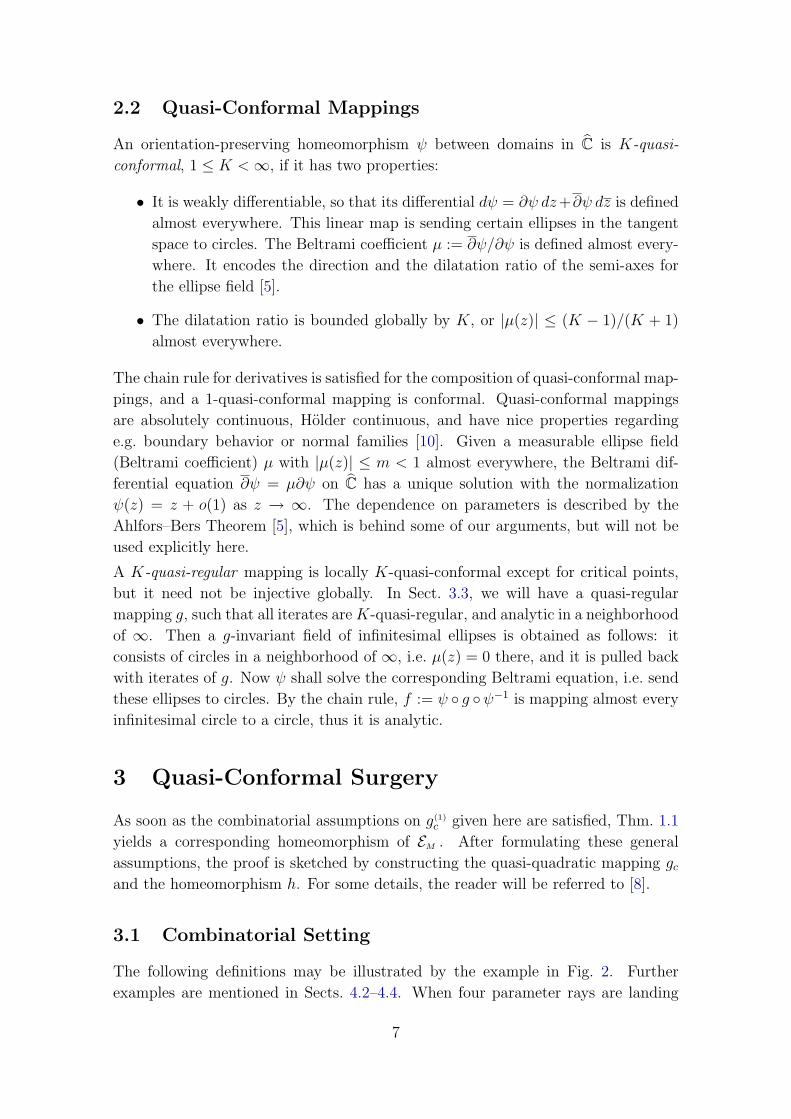
3.2 Construction of the Quasi-Quadratic Mapping gc

For c ∈ EM , we construct a quasi-regular mapping gc coinciding with g(1)c on Kc . By

employing the Boettcher conjugation Φc , the work will be done in the exterior of

the unit disk D. This is convenient when c ∈ EM , and essential to construct the

homeomorphism h in the exterior. In C \ Kc we have g(1)c = Φ−1

c G(1) Φc , where

G(1) : C\D → C\D is discontinuous on six straight rays, and given by compositions

of F (z) := z2 in the regions between these rays — it is independent of c in particular.

1. First construct smooth domains U, U ′ with D ⊂ U and U ⊂ U ′ , and a smooth

mapping G : U \ D → U ′ \ D. It shall be proper of degree 2 and coincide

with G(1) except in sectors around those six rays R(Θ±i ), where G(1) has a

shift discontinuity. The sectors are of the form | arg z− 2πΘ±i | < s log |z|, and

there G is chosen conveniently as a 1-homogeneous function of log z − i2πΘ±i ,

thus ensuring that the dilatation bound does not explode at the vertex of the

sector. (This simplifies the construction of [3], which employed a pullback

of quadrilaterals.) The domains are chosen in a finite recursion, employing

that some iterate of G(1) is strictly expanding [8, Sect. 5.2]. Since any orbit is

visiting at most two of the sectors, the dilatation of all iterates of G is bounded

uniformly.

2. Choose the radius R > 1 and the conformal mapping H : C \ U ′ → C \ DR2

with the normalization H(z) = z + O(1/z) at ∞ (which determines R and

H uniquely). Extend H to a quasi-conformal mapping H : C \ U → C \ DR

with F H = H G on ∂U . Define the extended G : C \ D → C \ D by

G := H−1 F H on C \ U . Now G is proper of degree 2, quasi-regular, and

the dilatation of Gn is bounded by some K uniformly in n. Finally, extend H

to a mappingH : C\D → C\D by recursive pullbacks, such that F H = HGeverywhere, then H is K-quasi-conformal. Cf. Fig. 4.

3. Now, set gc := g(1)c on Kc and gc := Φ−1

c G Φc on C \ Kc . Then gc is a

quasi-quadratic mapping, i.e. proper of degree 2, with a uniform bound on

the dilatation of the iterates, with ∂gc = 0 a.e. on Kc , and analytic in a

neighborhood of ∞ with gc(z) = z2 + O(1). (It is continuous at γc(Θ±i ) by

Lindelof’s Theorem.)

Now suppose that c ∈ PM \ EM with ΦM(c) ∈ U ′. Then Kc is totally disconnected,

and Φc is not defined in all of C \ Kc . It can be defined, however, in a domain

mapped to the six sectors and to C \ U by Φc [3, 8]. Thus gc is defined in this case

as well, by matching g(1)c with Φ−1

c G Φc .

In the following section, we shall construct an invariant ellipse field for the quasi-

quadratic gc , and employ it to straighten gc , i.e. to conjugate it to a quadratic

polynomial fd . Then we set h(c) := d. If we had skipped step 2, gc would not

be a quasi-quadratic mapping C → C, but a quasi-regular quadratic-like mapping

9

C \ D

C \ D

F (z) = z2

?

C \ D

C \ D

G

?

C \ Kc

C \ Kc

gc

?

C \ Kd

C \ Kd

fd

?

H

H

Φc

Φc

ψc-

ψc

-

Φd

Φd

K

Figure 4: Construction and straightening of gc by employing mappings in the exterior ofthe unit disk. If the filled Julia sets are not connected, the diagram is well-defined andcommuting on smaller neighborhoods of ∞.

(cf. [6, 8]) between bounded domains Uc → U ′c . This distinction is related to possible

alternative techniques:

Remark 3.2 (Alternative Techniques)

1. The classical techniques would be as follows [1, 2]: after the quasi-regular

quadratic-like mapping gc : Uc → U ′c is constructed, it is not extended to C, but

it is first conjugated to an analytic quadratic-like mapping, employing an invariant

ellipse field in U ′c . Then the latter mapping is straightened to a polynomial by the

Straightening Theorem [6]. With this approach, it will not be possible to extend

the homeomorphism h to the exterior of M.

2. Here we shall use the same techniques as in [3]: having extended gc to C, it will

be easy to straighten. Instead of applying the Straightening Theorem, its proof [5]

was adapted into the construction of gc . This approach makes the extension of h

to the exterior of M possible. By applying this technique to the construction of

gc and h(c) for c ∈ EM as well, the proofs of bijectivity, continuity, and of landing

properties (Sect. 4.1) are simplified.

3. Alternatively, gc : Uc → U ′c could be constructed as a quasi-regular quadratic-

like mapping on a bounded domain, and be straightened without extending it to Cfirst, by incorporating the alternative proofs of the Straightening Theorem according

to [6]. This proof is more involved, but it has the advantage that the mapping H

can be chosen more freely on U ′ \ U , e.g. such that it is the identity on R(Θ±1 )

and R(Θ±4 ) [8]. Then h would be the identity on the corresponding parameter rays,

which makes it easier to paste different homeomorphisms together.

10

3.3 h is a Homeomorphism

For c ∈ EM , or c ∈ PM \ EM with ΦM(c) ∈ U ′, the quasi-quadratic mapping gc was

constructed in the previous section. Now construct the gc-invariant ellipse field µ

by pullbacks with gc , such that µ = 0 in a neighborhood of ∞ and a.e. on Kc . It is

bounded by (K − 1)/(K + 1), since the dilatation of all iterates gnc is bounded by

K. Denote by ψc the solution of the Beltrami equation ∂ψ = µ∂ψ, normalized by

ψc(z) = z + O(1/z), which is mapping the infinitesimal ellipses described by µ to

circles. Now ψc gc ψ−1c is analytic on C and proper of degree 2, thus a quadratic

polynomial of the form fd(z) = z2 + d. In a neighborhood of ∞, H Φc ψ−1c is

conjugating fd to F , cf. Fig. 4. By the uniqueness of the Boettcher conjugation,

this mapping equals Φd . Recursive pullbacks show equality in C \Kd , if Kc and Kd

are connected, i.e. for c ∈ EM . Otherwise, equality holds on an fd-forward-invariant

domain of Φd , which may be chosen to include the critical value d.

We set h(c) := d = ψc(c). If c ∈ EM , a combinatorial argument shows d ∈ EM . If

c ∈ PM \ EM with ΦM(c) ∈ U ′, we have

ΦM(d) = Φd(d) = Φd ψc(c) = H Φc(c) = H ΦM(c) . (2)

Denote by PM the closed strip that is bounded by the four curves Φ−1M H(R(Θ±

i )),

i = 1, 4, which are quasi-arcs. Now h is extended to h : PM → PM by setting

h := Φ−1M H ΦM : PM \ EM → PM \ EM . (3)

By (2), this agrees with the definition of h(c) by straightening gc , if ΦM(c) ∈ U ′.

Now (3) shows that h is bijective and K-quasi-conformal in the exterior of EM . We

will see that h is bijective and continuous on EM . Let us remark that for c ∈ EM ,

the value of d = h(c) does not depend on the choices made in the construction of G

and H, since ψc is a hybrid-equivalence [6]. The proof of bijectivity in [2] relied on

this independence, but the following one is simplified by employing H:

For d ∈ EM , consider g(1)

d according to Def. 3.1, and define the quasi-quadratic

mapping gd with gd := g(1)

d on Kd and gd := Φ−1d G Φd in C \ Kd , where G :=

H F H−1. To see that this choice is possible, note that H is mapping the

region V ⊂ U \ D (corresponding to Vc) to a distorted version of V . There we have

G(1) = F 2−kv (±F kv−1). Observing that F = H G H−1 and H commutes with

±id on the set in question, we have G(1) = H G2−kv (±Gkv−1) H−1. Following

the orbit and applying the piecewise definition of G(1) yields G(1) = H F H−1.

Together with the same result in other regions, this justifies the definition of G,

i.e. gd is quasi-quadratic. Now h(d) is defined by straightening gd . — Suppose that

c ∈ EM and d = h(c), then fd = ψc gc ψ−1c and by its definition in terms of

H = Φd ψc Φ−1c , we have gd = ψc fc ψ−1

c . Therefore c = h(d) and ψd = ψ−1c .

h h = id and the converse result imply that h : EM → EM is bijective with h−1 = h.

By (3), h is quasi-conformal in the exterior of EM . The interior of EM consists of

a countable family of hyperbolic components, plus possibly a countable family of

11

non-hyperbolic components. The former are parametrized by multiplier maps, the

latter by transforming invariant line fields. In both cases, h is given by a composition

of these analytic parametrizations [2, 8]. It remains to show that h is continuous

at c0 ∈ ∂EM : suppose cn → c0 , dn = h(cn), d0 = h(c0). By bijectivity we have

d0 ∈ ∂EM = EM∩∂M. It does not matter if cn belongs to EM or not. (Now we employ

the definition of h by straightening gc , which is equivalent to (3). One special case

requires extra treatment: when some γc(Θ±i ) is iterated to γc(Θ

±1 ), and c0 = γM(Θ±

i ),

then gc0 is not defined.) It is sufficient to show dn → d∗ ⇒ d∗ = d0 . Since the K-

quasi-conformal mappings ψn are normalized, there is a K-quasi-conformal Ψ and a

subsequence ψc′n → Ψ, uniformly on C [10]. We have ψc′n gc′n ψ−1c′n→ Ψ gc0 Ψ−1

and ψcn gcn ψ−1cn

= fdn → fd∗ , thus Ψ ψ−1c0

is a quasi-conformal conjugation from

fd0 to fd∗ . Although it need not be a hybrid-equivalence, d0 ∈ ∂M implies d∗ = d0

[6]. By the same arguments, or by the Closed Graph Theorem, h−1 is continuous as

well. Thus h : PM → PM is a homeomorphism mapping EM → EM .

3.4 Further Properties of h

Since h is analytic in the interior of EM and quasi-conformal in the exterior, it is

natural to ask if it is quasi-conformal everywhere. Branner and Lyubich are working

on a proof employing quasi-regular quadratic-like germs. Maybe an alternative proof

can be given by constructing a homotopy from fc to gd , thus from id to h.

The dynamics of h on EM is simple: set c0 := γM(Θ±2 ) and cn := hn(c0), n ∈ Z.

The connected component of EM between the two pinching points cn and cn+1 is a

fundamental domain for h±1. These are accumulating at the Misiurewicz points a

and b, and the method of [17] yields a linear scaling behavior. Thus h and h−1 are

Lipschitz continuous at a and b (and Holder continuous at all Misiurewicz points).

For c ∈ EM \ a, b we have hn(c) → b as n→∞ and hn(c) → a as n→ −∞.

4 Related Results and Possible Generalizations

Further results and examples from [8] are sketched, and we present some ideas on

surgery for general one-parameter families.

4.1 Combinatorial Surgery

The unit circle ∂D is identified with S1 := R/Z by the parametrization exp(i2πθ).

For h constructed from g(1)c according to Thm. 1.1, recall the mappings F, G, H :

C\D → C\D from Sect. 3.2. Denote their boundary values by F, G, H : S1 → S1.

Thus F(θ) = 2θmod 1 and G is piecewise linear. Now H is the unique orientation-

preserving circle homeomorphism conjugating G to F, H G H−1 = F. H(θ)

is computed numerically from the orbit of θ under G as follows: for n ∈ N, the

12

n-th binary digit of H(θ) is 0 if 0 ≤ Gn−1(θ) < 1/2, and 1 if 1/2 ≤ Gn−1(θ) < 1.

For rational angles, the (pre-) periodic sequence of digits is obtained from a finite

algorithm.

In the exterior of EM , h is represented by H according to (3). Applying this formula

to parameter rays and employing Lindelof’s Theorem shows: RM(θ) is landing at

c ∈ ∂EM , iff RM(H(θ)) is landing at h(c). If c is a Misiurewicz point or a root, then

θ is rational, and H(θ) is computed exactly. In this sense, d = h(c) is determined

combinatorially. Alternatively, one can construct the critical orbit of g(1)c and the

Hubbard tree of fd . The simplest case is given when the critical orbit meets Ec only

once: then the orbit of c under g(1)c is the same as the orbit of ηc(c) under fc .

Regularity properties of H are discussed in [8, Sect. 9.2]. H has Lipschitz or Holder

scaling properties at all rational angles. H and H−1 are Holder continuous with

the optimal exponents kv/kv and kw/kw . Since H is K-quasi-conformal, Mori’s

Theorem [10] says that H±1 is 1/K-Holder continuous. Thus we have the lower

boundK ≥ max(kv/kv, kw/kw), independent of the choices made in the construction

of h : PM \EM → PM \EM . By a piecewise construction we obtain a homeomorphism

h : M→M, which extends to a homeomorphism of C, but such that no extension

can be quasi-conformal.

4.2 Homeomorphisms at Misiurewicz Points

A homeomorphism h : EM → EM according to Thm. 1.1 is expanding at the Misi-

urewicz point a. Asymptotically, M shows a linear scaling behavior at a. (In Fig. 3,

you can observe the asymptotic self-similarity of M at a, and similarity between

M at c ≈ cn and Kcn at z ≈ 0.) Now h is asymptotically linear in a “macroscopic”

sense, e.g. there is an asymptotically linear sequence of fundamental domains, but

this is not true pointwise. These results are obtained by combining the techniques

from [17] with the combinatorial description of h according to Sect. 4.1: consider a

suitable sequence cn → a. If the critical orbit of fcn travels through Ecn once, then

h is asymptotically linear on the sequence, but it is not if the orbit meets Ecn twice.

Conversely, given a branch at some Misiurewicz point a, is there an appropriate

homeomorphism h? We only need to find a combinatorial construction of g(1)c . This

is done in [8] e.g. for all β-type Misiurewicz points. (Here PM and Vc ∪Wc are sectors,

not strips.) The author’s research was motivated by discussions with D. Schleicher,

who had worked on the construction of dynamics in the parameter plane before.

4.3 Edges, Frames, and Piecewise Constructions

For parameters c in the p/q-limb of M, the filled Julia set Kc has q branches at the

fixed point αc of fc . A connected subset Ec ⊂ Kc is a dynamic edge of order n, if

fn−1c is injective on Ec and fn−1

c (Ec) is the part of Kc between αc and −αc . (More

precisely, fn−1c shall be injective in a neighborhood of the edge without its vertices.)

13

The edge is characterized by the external angles at the vertices. As c varies, it may

still be defined, or it may cease to exist after a bifurcation of preimages of αc . Now

EM ⊂ Mp/q is a parameter edge, if for all c ∈ EM the dynamic edge Ec (with given

angles) exists and satisfies c ∈ Ec , and if EM has the same external angles as Ec . In

Figs. 2–3, EM is the parameter edge of order 4 in M1/3 .

Mp/q contains a little Mandelbrot set M′ = c0 ∗ M of period q (cf. Sect. 4.4). If

a parameter edge EM is behind c0 ∗ (−1), there is a homeomorphism h : EM → EM

analogous to that of Figs. 2–3. Behind the α-type Misiurewicz point c0 ∗ (−2),

edges can be decomposed into subedges and frames [8, Sect. 7]. These frames are

constructed recursively, like the intervals in the complement of the middle-third

Cantor set. A family of homeomorphisms on subedges shows that all frames on the

same edge are mutually homeomorphic, and they form a finer decomposition than

the fundamental domains of a single homeomorphism. By permuting the frames

(in a monotonous way), new homeomorphisms h are defined piecewise. These may

have properties that are not possible when h is constructed from a single surgery.

E.g., in contradiction to Sect. 3.4, h can be constructed such that it is not Lipschitz

continuous or not even Holder continuous at the vertex a of EM . Or it can map a

Misiurewicz point with two external angles to a parameter with irrational angles,

which is not a Misiurewicz point.

The notions of edges and frames can be generalized: for parameters c behind the

root of a hyperbolic component, the filled Julia set Kc contains two corresponding

pre-characteristic points, which take the roles of ±αc .

4.4 Tuning and Composition of Homeomorphisms

For a center c0 of period p, there is a “little Mandelbrot set” M′ ⊂M and a tuning

map M → M′, x 7→ y = c0 ∗ x with 0 7→ c0 . Now Ky contains a “little Julia

set” Ky, p around 0, where fpy is conjugate to fx on Kx [6, 7]. A homeomorphism

h : EM → EM according to Thm. 1.1 is compatible with tuning in two different ways:

• If c0 ∈ EM , then h is mapping M′ to the little Mandelbrot set at h(c0):

h(c0 ∗ x) = (h(c0)) ∗ x. Cf. [2].

• For any center c0 ∈ M, set E ′M := c0 ∗ EM ⊂ M. A new homeomorphism

h′ : E ′M → E ′M is obtained by composition, i.e. h′(c0 ∗x) := c0 ∗ (h(x)). Now E ′Mis obtained by disconnecting M at a countable family of pinching points, but

h′ has a natural extension to all of these “decorations” (except for two): the

mapping ηc that produced the homeomorphism h is transferred by cutting the

little Julia set into strips. The required pinching points do not bifurcate when

the parameter y is in a decoration of E ′M , thus the new piecewise construction

η′y works in a whole strip. An example is shown in Fig. 5 (left).

14

The same principle applies, e.g., to crossed renormalization [12], or to the Branner-

Douady homeomorphism ΦA : M1/2 → T ⊂ M1/3 : suppose that EM ⊂ M1/2 and

h : EM → EM is constructed according to Thm. 1.1, i.e. from a combinatorial g(1)c

according to Def. 3.1. Then E ′M := ΦA(EM) is a subset of M1/3, where a countable

family of decorations was cut off. Again h′ := ΦA h Φ−1A : E ′M → E ′M extends to

a whole strip by transferring the combinatorial construction of g(1)c . If, e.g., h is a

suitable homeomorphism on the edge from γM(5/12) to γM(11/24), then h′ is the

homeomorphism of Figs. 2, 3.

a

b

@@

@@I h′

a

b

h′

Figure 5: Two homeomorphisms h′ : E ′M → E ′M obtained from a similar construction ash : EM → EM in Figs. 2–3. Left: tuning with the center c0 = −1 yields an edge in the limbM1/2 ⊂M. The eight angles Θ±

i are obtained by tuning those of Fig. 2, i.e. replacing thedigits 0 by 01 and 1 by 10. h′ is defined not only on c0 ∗ EM , but on a strip including alldecorations. Right: part of the parameter space of cubic polynomials with a persistentlyindifferent fixed point. The connectedness locus contains copies of a quadratic Siegel Juliaset [4]. Again, h′ is defined in a strip containing a countable family of decorations attachedto the copy of EM .

4.5 Other Parameter Spaces

In Thm. 1.1 we obtained homeomorphisms h : EM → EM of suitable subsets EM ⊂M,

but the method is not limited to quadratic polynomials. To apply it to other one-

dimensional families of polynomials or rational mappings, these mappings must be

characterized dynamically. The polynomials of degree d form a (d− 1)-dimensional

family (modulo affine conjugation). Suppose that a one-dimensional subfamily fc is

defined by one or more of the following critical relations :

• A critical point of fc is degenerate, or one critical point is iterated to another

one, or critical orbits are related by fc being even or odd.

• A critical point is preperiodic or periodic (superattracting).

• There is a persistent cycle with multiplier ρ, 0 < |ρ| ≤ 1. This cycle is always

“catching” one of the critical points, but the choice may change.

15

An appropriate combination of such relations defines a one-parameter family fc ,

where the coefficients and the critical points of fc are algebraic in c. Locally in the

parameter space, there is one active or free critical point ωc , whose orbit determines

the qualitative dynamics. The other critical points are either linked to ωc , or their

behavior is independent of c. The connectedness locus Mf contains the parameters

c, such that the filled Julia set Kc of fc is connected, equivalently fnc (ωc) 6→ ∞, or

ωc ∈ Kc . In general ωc is not defined globally by an analytic function of c, since

it may be a multi-valued algebraic function of c, or since a persistent cycle may

catch different critical points. But looking at specific families, it will be possible to

define ΦM and parameter rays for suitable subsets of the parameter space, and to

understand their landing properties.

Then an analogue of Thm. 1.1 can be proved: for a piecewise defined g(1)c , a quasi-

polynomial mapping gc is constructed analogously to Sect. 3.2, and straightened to

a polynomial. By the critical relations and by normalizing conditions, it will be of

the form fd , and we set h(c) := d. (At worst, the normalizing conditions will allow

finitely many choices for d.) Note that this procedure will not work, if our family

fc is an arbitrary submanifold of the (d− 1)-dimensional family of all polynomials,

and not defined by critical relations.

When such a theorem is proved, the remaining creative step is the combinatorial

definition of EM and g(1)c . Some examples can be obtained in the following way: when

a non-degenerate critical point is active, the connectedness locus Mf will contain

copies M′ of M [11]. Starting from a homeomorphism h : EM → EM , M′ contains

a decorated copy of EM , and the corresponding homeomorphism h′ extends to all

decorations by an appropriate definition of g(1)c — the angles Θ±

i are seen at the

copy of a quadratic Julia set within Kc , where some iterate of fc is conjugate to

a quadratic polynomial. It remains to check that no other critical orbit is passing

through Vc ∪Wc , then g(1)c is well-defined. An example is given in Fig. 5 (right).

The rational mappings of degree d form a (2d − 2)-dimensional family (modulo

Mobius conjugation). Suppose that a one-dimensional subfamily fc is defined by

critical relations. When there are one or more persistently (super-) attracting cycles,

then Kc shall be the complement of the basin of attraction, and Mf shall contain

those parameters, such that the local free critical point is not attracted. ∂Mf will be

the bifurcation locus [11]. If the persistent cycles are superattracting, we can define

dynamic rays and parameter rays by the Boettcher conjugation. When the topology

and the landing properties are understood sufficiently well, homeomorphisms can be

constructed by quasi-conformal surgery.

An example is provided by cubic Newton methods, cf. [6, 18, 14]: fc has three

superattracting fixed points and one free critical point. Parts of the parameter

space are shown in Fig. 6. By dynamic rays in the adjacent immediate basins of

two fixed points, the Julia set is cut into “strips” to define g(1)c . In both basins,

the techniques of Sect. 3.2 are applied to construct the quasi-Newton mapping gc .

It is straightened to fd , and a homeomorphism is obtained by h0(c) := d. It is

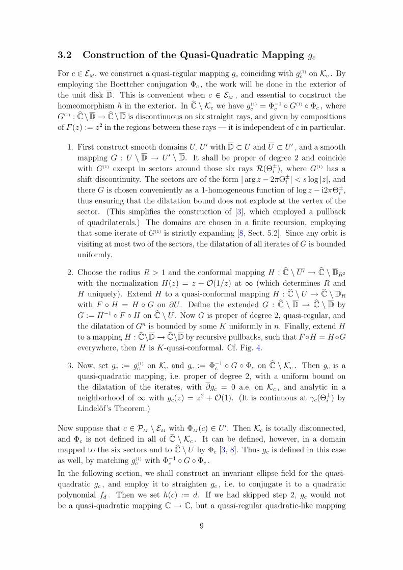
16

permuting little “almonds,” respecting their decomposition into four colors. Similar

constructions are possible when one or both of the adjacent components of basins

at Ec are not immediate, i.e. when the hyperbolic components at EM are of greater

depth [14]. Cf. h1 , h2 in Figs. 6–7.

?

h0

h1

6h2

Figure 6: Homeomorphisms in the parameter space of Newton methods for cubic polyno-mials. Left: an “edge” between the “almonds” of orders 3 and 2. Right: homeomorphismson edges within the almond of order 2. (The different colors, or shades of gray, indicatethat the free critical point is attracted to one of the roots of the corresponding polynomial.)

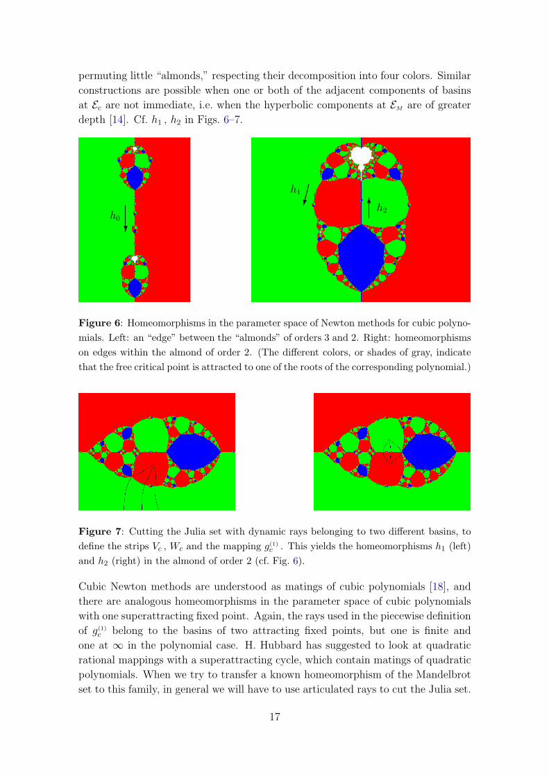
Figure 7: Cutting the Julia set with dynamic rays belonging to two different basins, todefine the strips Vc , Wc and the mapping g(1)

c . This yields the homeomorphisms h1 (left)and h2 (right) in the almond of order 2 (cf. Fig. 6).

Cubic Newton methods are understood as matings of cubic polynomials [18], and

there are analogous homeomorphisms in the parameter space of cubic polynomials

with one superattracting fixed point. Again, the rays used in the piecewise definition

of g(1)c belong to the basins of two attracting fixed points, but one is finite and

one at ∞ in the polynomial case. H. Hubbard has suggested to look at quadratic

rational mappings with a superattracting cycle, which contain matings of quadratic

polynomials. When we try to transfer a known homeomorphism of the Mandelbrot

set to this family, in general we will have to use articulated rays to cut the Julia set.

17

Although it may be possible to define g(1)c , it will not be possible to construct the

quasi-regular mapping gc , because the shift discontinuity happens not only within

the basin of attraction, but at pinching points of the Julia set as well. For the same

reason, it will not be possible to transfer a homeomorphism of M to a neighborhood

of a copy of M in the cubic Newton family.

5 Homeomorphism Groups of M

Denote the group of orientation-preserving homeomorphisms h : M →M by GM .

If two homeomorphisms coincide on ∂M, they encode the same information on the

topological structure of M. To avoid trivialities, we suggest some definitions of

groups of non-trivial homeomorphisms as well.

Definition 5.1 (Groups of Homeomorphisms)

1. GM is the group of homeomorphisms h : M→M that are orientation-preserving

at branch points, and orientation-preserving in the interior of M.

2. Ga is the group of homeomorphisms h : M→M that are orientation-preserving

at branch points, and analytic in the interior of M.

3. Gb is the group of homeomorphisms h : ∂M→ ∂M that are orientation-preserving

at branch points, and orientation-preserving on the boundaries of hyperbolic compo-

nents.

4. Gq is the factor group GM/G1 , where G1 is the normal subgroup consisting of trivial

homeomorphisms: G1 := h ∈ GM |h = id on ∂M.

Gq is the most natural definition of non-trivial homeomorphisms. Ga , Gb , Gq may

well turn out to be mutually isomorphic. On GM , Ga , and Gb , define a metric by

d(h1, h2) := ‖h1 − h2‖∞ + ‖h−11 − h−1

2 ‖∞ (4)

:= max |h1(c)− h2(c)|+ max |h−11 (c)− h−1

2 (c)| ,

where the maxima are taken over c ∈ M or c ∈ ∂M, respectively. Gq consists of

equivalence classes of homeomorphisms coinciding on the boundary, [h] = hG1 =

G1h. Since G1 is closed, a metric is given by

d([h1], [h2]) := inf‖h′1 − h′2‖∞

∣∣∣h′1 ∈ [h1], h′2 ∈ [h2]

+ inf

‖h′1

−1 − h′2−1‖∞

∣∣∣h′1 ∈ [h1], h′2 ∈ [h2]

(5)

= inf‖h1 u− h2‖∞ + ‖h−1

1 v − h−12 ‖∞

∣∣∣u, v ∈ G1

. (6)

It may be more natural to take the infimum of a sum instead of the sum of infima

in (5), i.e. inf d(h′1, h′2), but I do not know how to prove the triangle inequality in

that case. (6) is obtained from (5) by employing the facts that G1 is normal, and

that right translations are isometries of the norm: ‖h1−h2‖∞ = ‖h1 h−h2 h‖∞ ,

since h ∈ GM is bijective.

18

Proposition 5.2 (Topology of Homeomorphisms Groups)

1. GM , Ga , Gb , Gq are complete metric spaces and topological groups, i.e. composi-

tion and inversion are continuous.

2. For G = GM , Ga , Gb , Gq we have: if Ω1 , Ω2 are hyperbolic components, then

N := h ∈ G |h(∂Ω1) = ∂Ω2 is open.

Proof : 1. For GM , Ga , Gb , the proof is straightforward. But suppose we had

used the alternative metric d(h1, h2) := ‖h1 − h2‖∞ , and (hn) ⊂ GM is a Cauchy

sequence in that metric. Then it is converging uniformly to a continuous, surjective

h : EM → EM . If h is injective, then h−1n → h−1 uniformly. But h need not be

injective, a counterexample is constructed in item 2 of [8, Prop. 7.7]. Thus, if we

had used d instead of d, the topology of GM , Ga , Gb would be the same, but they

would be incomplete metric spaces.

Now suppose ([hn]) is a Cauchy sequence in Gq . It is sufficient to show that a sub-

sequence converges, and without restriction we have d([hn+1], [hn]) ≤ 3−n. Choose

un , vn ∈ G1 with

‖hn+1 un − hn‖∞ ≤ 2−n and ‖h−1n+1 vn − h−1

n ‖∞ ≤ 2−n .

Define the sequences

hn := hn un−1 un−2 . . . u1 and hn := h−1n vn−1 vn−2 . . . v1 .

Since the maximum norm is invariant under right translations on M, they satisfy

‖hn+1 − hn‖∞ ≤ 2−n and ‖hn+1 − hn‖∞ ≤ 2−n ,

and there are continuous functions h, h with hn → h and hn → h uniformly. Now

h h and h h are uniform limits of a sequence in G1 , thus surjective, and h is a

homeomorphism. We have hn → h in GM and [hn] = [hn] → [h] in Gq , therefore Gq

is complete.

2. Hyperbolic components can be distinguished topologically from non-hyperbolic

components, since only the boundary of a hyperbolic component contains a count-

able dense set of pinching points (by the Branch Theorem [15]). Thus every homeo-

morphism of M or ∂M is permuting the set of hyperbolic components or of their

boundaries, respectively. Fix a, b ∈ ∂Ω2, and choose ε > 0 such that no hyperbolic

component 6= Ω2 is meeting both of the disks of radius ε around a and b. This

is possible, since there are several external rays landing at ∂Ω2 . If h0 ∈ N and

h ∈ G with d(h, h0) < ε, then |h(h−10 (a)) − a| < ε and |h(h−1

0 (b)) − b| < ε, thus

h(∂Ω1) = ∂Ω2 . (Analogously for the classes in Gq .)

Theorem 5.3 (Groups of Non-Trivial Homeomorphisms)

The groups of non-trivial homeomorphisms of M or ∂M — Ga , Gb and Gq — share

the following properties:

1. They have the cardinality of the continuum R, and they are totally disconnected.

19

2. They are perfect, and not compact (not even locally compact).

3. A family of homeomorphisms F ⊂ Ga , Gb , Gq is called normal, if its closure is

sequentially compact. A necessary condition is that for every hyperbolic component

Ω ⊂M, there are only finitely many components of the form h±1(Ω), h ∈ F . If Mis locally connected, this condition will be sufficient for F being normal.

By composition, the homeomorphisms constructed by surgery according to Thm. 1.1

generate a countable subgroup of Ga , Gb or Gq . Will it be dense? — For GM , items 1

and 3 are wrong, and item 2 is true but trivial. Hence the motivation to consider

the groups of non-trivial homeomorphisms. The same results hold for the analogous

groups, where the condition of preserving the orientation is dropped.

Proof: We prove the statements for Ga , the case of Gb or Gq is similar. There is a

sequence of disjoint subsets En ⊂M with diam(En) → 0, and a sequence of analytic

homeomorphisms hn : M→M, such that hn = id onM\En , hn 6= id. To construct

these, fix a homeomorphism h∗ : EM → EM according to Thm. 1.1, e.g. that of Figs. 2

and 3. Choose E0 ⊂ EM and a homeomorphism h0 : E0 → E0 , h0 6= id, such that

E0 is contained in a fundamental domain of h∗ . This is possible e.g. by the tuning

construction from Sect. 4.4. Then set hn := hn∗ h0 h−n

∗ on En := hn∗ (E0), and

extend it by the identity to a homeomorphism of M. We have diam(En) → 0 by the

scaling properties of M at Misiurewicz points [17]. — An alternative approach is as

follows: construct homeomorphisms hn : En → En , such that En is contained in the

limb M1/n , then diam(En) → 0 by the Yoccoz inequality. These homeomorphisms

can be constructed by tuning, or at β-type Misiurewicz points according to Sect. 4.2,

or on edges (Sect. 4.3). All of the homeomorphisms constructed below extend to

homeomorphisms of C, cf. item 3 of Remark 3.2. (If M is locally connected, all

homeomorphisms in GM , Ga or Gb extend to homeomorphisms of C.)

1. We construct an injection (0, 1) → Ga , x 7→ h as follows: expand x in binary

digits (not ending on 1). Set h := hn or h := id on En , if the n-th digit is 1 or

0, respectively, and h := id on M \ ⋃ En . Although the sequence of sets En will

accumulate somewhere, continuity of h can be shown by employing diam(En) → 0.

— Conversely, to obtain an injection Ga → (0, 1), h 7→ x, enumerate the hyperbolic

components (Ωn)n∈N, and denote the n-th prime number by pn . Now x shall have

the digit 1 at the place pmn , iff h : Ωn → Ωm . The mapping h 7→ x is injective, since

the homomorphism from Ga to the permutation group of hyperbolic components

is injective: if h is mapping every hyperbolic component to itself, it is fixing the

points of intersection of closures of hyperbolic components, i.e. all roots of satellite

components. These are dense in ∂M, thus h = id. — By the two injections,

|Ga| = |(0, 1)| = |R|.If h1, h2 ∈ Ga with h1 6= h2 , there is a hyperbolic component Ω with h1(Ω) 6= h2(Ω).

By Prop. 5.2, N := h ∈ Ga |h(Ω) = h1(Ω) is an open neighborhood of h1 , and

Ga \ N =⋃h ∈ Ga |h(Ω) = Ω′ is an open neighborhood of h2 , where the union

is taken over all hyperbolic components Ω′ 6= h1(Ω). Thus h1 and h2 belong to

20

different connected components, and Ga is totally disconnected.

2. We have d(hn , id) ≤ 2 diam(En) → 0 as n → ∞, thus id is not isolated in Ga .

Since composition is continuous, no point is isolated, and Ga is perfect.

Choose a homeomorphism h : EM → EM according to Thm. 1.1, which is expanding

at a and contracting at b, extend it by the identity to h ∈ Ga . The iterates of h

satisfy hk(a) = a and hk(c) → b for all c ∈ EM \ a, thus the pointwise limit of

(hk)k∈N is not continuous. The sequence does not contain a subsequence converging

uniformly, and Ga is not sequentially compact, a fortiori not compact. — If N is a

neighborhood of id in Ga , fix an n such that N contains the ball of radius 2 diam(En)

around id, then N contains the sequence (hkn)k∈N. Thus N is not compact, and Ga

is not locally compact.

3. When F does not satisfy the finiteness condition, there is a sequence (hn) ⊂ Fand a hyperbolic component Ω, such that the period of hn(Ω) (or h−1

n (Ω)) diverges.

Assume hn → h, then hn(Ω) = h(Ω) for n ≥ N0 according to Prop. 5.2, a con-

tradiction. If F satisfies the finiteness condition, a diagonal procedure yields a

subsequence which is eventually constant on every hyperbolic component, thus re-

specting the partial order of hyperbolic components. Assuming local connectivity,

all fibers are trivial [15], and limhn is obtained analogously to [8, Sect. 9.3].

Two rational angles with odd denominators are Lavaurs-equivalent, if the corre-

sponding parameter rays are landing at the same root. Denote the closure of this

equivalence relation on S1 by ∼. The abstract Mandelbrot set is the quotient space

S1/ ∼ [9], it is a combinatorial model for ∂M, which will be homeomorphic to

∂M if M is locally connected. (It is analogous to Douady’s pinched disk model

of M.) Orientation-preserving homeomorphisms of the abstract Mandelbrot set are

described by orientation-preserving homeomorphisms H : S1 → S1 that are compat-

ible with ∼. According to Sect. 4.1, every homeomorphism h : EM → EM constructed

by surgery defines such a circle homeomorphism (extended by the identity), and the

homeomorphism group of S1/∼ has the properties given in Thm. 5.3. In fact, these

homeomorphisms of the abstract Mandelbrot set can be constructed in a purely

combinatorial way, without using quasi-conformal surgery [8].

References

[1] B. Branner, A. Douady, Surgery on complex polynomials, in: Holomorphic dynamics,Proc. 2nd Int. Colloq. Dyn. Syst., Mexico City, LNM 1345, 11–72 (1988).

[2] B. Branner, N. Fagella, Homeomorphisms between limbs of the Mandelbrot set,J. Geom. Anal. 9, 327–390 (1999).

[3] B. Branner, N. Fagella, Extensions of Homeomorphisms between Limbs of the Man-delbrot Set, Conform. Geom. Dyn. 5, 100–139 (2001).

21

[4] X. Buff, C. Henriksen, Julia sets in parameter spaces, Comm. Math. Phys. 220,333–375 (2001).

[5] L. Carleson, T. W. Gamelin, Complex dynamics, Springer, New York, 1993.

[6] A. Douady, J. H. Hubbard, On the dynamics of polynomial-like mappings, Ann. Sci.Ecole Norm. Sup. 18, 287–343 (1985).

[7] P. Haıssinsky, Modulation dans l’ensemble de Mandelbrot, in: The Mandelbrot Set,Theme and Variations, Tan L. ed., LMS Lecture Notes 274, Cambridge UniversityPress 2000.

[8] W. Jung, Homeomorphisms on Edges of the Mandelbrot Set, Ph.D. thesis RWTHAachen 2002.

[9] K. Keller, Invariant Factors, Julia Equivalences and the (Abstract) Mandelbrot Set,LNM 1732, Springer 2000.

[10] O. Lehto, K. I. Virtanen, Quasiconformal Mappings in the Plane, Springer 1973.

[11] C. T. McMullen, The Mandelbrot set is universal, in: The Mandelbrot Set, Themeand Variations, Tan L. ed., LMS Lecture Notes 274, Cambridge University Press2000.

[12] J. Riedl, D. Schleicher, On Crossed Renormalization of Quadratic Polynomials, in:Proceedings of the 1997 conference on holomorphic dynamics, RIMS Kokyuroku1042, 11–31, Kyoto 1998.

[13] J. Riedl, Arcs in Multibrot Sets, Locally Connected Julia Sets and Their Constructionby Quasiconformal Surgery, Ph.D. thesis TU Munchen 2000.

[14] P. Roesch, Topologie locale des methodes de Newton cubiques, Ph.D. thesis ENS deLyon 1997.

[15] D. Schleicher, On Fibers and Local Connectivity of Mandelbrot and Multibrot Sets,IMS-preprint 98-13a (1998).

[16] D. Schleicher, Rational Parameter Rays of the Mandelbrot Set, Asterisque 261, 405–443 (2000).

[17] Tan L., Similarity between the Mandelbrot set and Julia sets, Comm. Math. Phys.134, 587–617 (1990).

[18] Tan L., Branched coverings and cubic Newton maps, Fundam. Math. 154, 207–260(1997).

Present address: Wolf Jung, Inst. Reine Angew. Math.RWTH Aachen, D-52056 Aachen, Germanyhttp://www.iram.rwth-aachen.de/∼jungjung@iram.rwth-aachen.de

22