Embed Size (px)
Citation preview

Homework 2‐ ee 662
Author:
Collaborators:
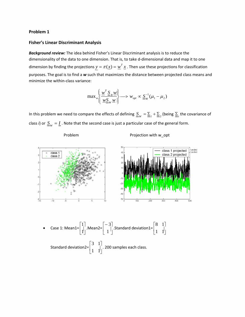
Problem 1
Fisher’s Linear Discriminant Analysis
Background review: The idea behind Fisher’s Linear Discriminant analysis is to reduce the dimensionality of the data to one dimension. That is, to take d‐dimensional data and map it to one
dimension by finding the projections xwxy T== )(π . Then use these projections for classification
purposes. The goal is to find a w such that maximizes the distance between projected class means and minimize the within‐class variance:
⎪⎭
⎪⎬⎫
⎪⎩
⎪⎨⎧
wSwwSw
W
BT
wmax ‐‐‐‐> )( 211 µµ −∝ −
Wopt Sw
In this problem we need to compare the effects of defining 21 Σ+Σ=W
S (being iΣ the covariance of
class i) or ISW
= . Note that the second case is just a particular case of the general form.
Problem Projection with w_opt
• Case 1: Mean1= ⎥⎦
⎤⎢⎣
⎡11
.Mean2= ⎥⎦
⎤⎢⎣
⎡−13
.Standard deviation1= ⎥⎦
⎤⎢⎣
⎡1118
Standard deviation2= ⎥⎦
⎤⎢⎣
⎡1113
. 200 samples each class.
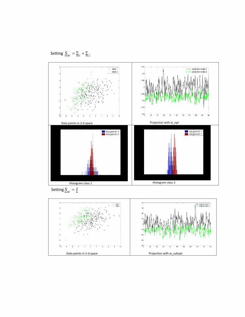
Setting 21 Σ+Σ=W
S
Data points in 2‐d space Projection with w_opt
Histogram class 1
Histogram class 2
Setting ISW
=
Data points in 2‐d space Projection with w_subopt
Histogram class 1
Histogram class 2
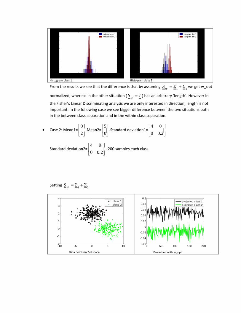
From the results we see that the difference is that by assuming 21 Σ+Σ=W
S we get w_opt
normalized, whereas in the other situation ( ISW
= ) has an arbitrary ‘length’. However in
the Fisher’s Linear Discriminating analysis we are only interested in direction, length is not important. In the following case we see bigger difference between the two situations both in the between class separation and in the within class separation.
• Case 2: Mean1= ⎥⎦
⎤⎢⎣
⎡20
.Mean2= ⎥⎦
⎤⎢⎣
⎡05
.Standard deviation1= ⎥⎦
⎤⎢⎣
⎡2.00
04
Standard deviation2= ⎥⎦
⎤⎢⎣
⎡2.00
04. 200 samples each class.
Setting 21 Σ+Σ=W
S
-10 -5 0 5 10-2
-1
0
1
2
3
4
class 1class 2
Data points in 2‐d space
0 50 100 150 200-0.06
-0.04
-0.02
0
0.02
0.04
0.06
0.08
0.1
projected class1projected class 2
Projection with w_opt
-30 -20 -10 0 10 20 300
10
20
30
40
50
histogram dim 1histogram dim 2
Histogram class 1
-30 -20 -10 0 10 20 300
10
20
30
40
50
60
histogram dim 1histogram dim 2
Histogram class 2
Setting ISW
=
-10 -5 0 5 10-2
-1
0
1
2
3
4
class 1class 2
Data points in 2‐d space
0 50 100 150 200-50
-40
-30
-20
-10
0
10
20
30
40
projected class 1projected class 2
Projection with w_subopt
-30 -20 -10 0 10 20 300
10
20
30
40
50
histogram dim 1histogram dim 2
Histogram class 1
-30 -20 -10 0 10 20 300
10
20
30
40
50
60
histogram dim 1histogram dim 2
Histogram class 2
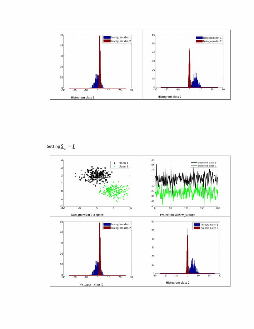
In this second case, when we set ISW
= the algorithm only optimizes this term: wSwB
T ,
and thus the dimension with larger |m_1‐m_2| will be choosen (larger between classes).
Also in the second situation ( ISW
= ) the algorithm does not take into consideration the
variance within class scatters; this is why we see clearly that in this situation the within projected classes plot is less compacted in comparison with the situation where we
set 21 Σ+Σ=W
S. Hence the results using the optimal Fisher’s solution show that the
classes are better separated. In the histograms provided we can see how different the distributions for the two cases are, and this leads us to a second case where the advantage of using the optimal Fisher’s solution is highlighted.
Problem 2
2.1 Neural Network classifier
Background review: In this section we have implemented an artificial multilayer neural network with one hidden network. This is the topology of our network:
Figure. Topology of our Neural Network
Our goal now is to set the weights based on the training patterns and the desired outputs. To do so, we have used the back‐propagation algorithm. This is based on the gradient descent in error:
• Select a network architecture
• Initialize the weights to small random values
• Compute the corresponding outputs according to the training set
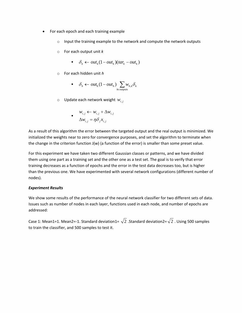
• For each epoch and each training example
o Input the training example to the network and compute the network outputs
o For each output unit k
))(1( kkkkk outtaroutout −−←δ
o For each hidden unit h
∑∈
−←outputsk
kkhhhh woutout δδ ,)1(
o Update each network weight jiw ,
jijji
jijiji
xwwww
,,
,,,
ηδ=∆
∆+←
As a result of this algorithm the error between the targeted output and the real output is minimized. We initialized the weights near to zero for convergence purposes, and set the algorithm to terminate when the change in the criterion function J(w) (a function of the error) is smaller than some preset value.
For this experiment we have taken two different Gaussian classes or patterns, and we have divided them using one part as a training set and the other one as a test set. The goal is to verify that error training decreases as a function of epochs and the error in the test data decreases too, but is higher than the previous one. We have experimented with several network configurations (different number of nodes).
Experiment Results
We show some results of the performance of the neural network classifier for two different sets of data. Issues such as number of nodes in each layer, functions used in each node, and number of epochs are addressed:
Case 1: Mean1=1. Mean2=‐1. Standard deviation1= 2 .Standard deviation2= 2 . Using 500 samples to train the classifier, and 500 samples to test it.
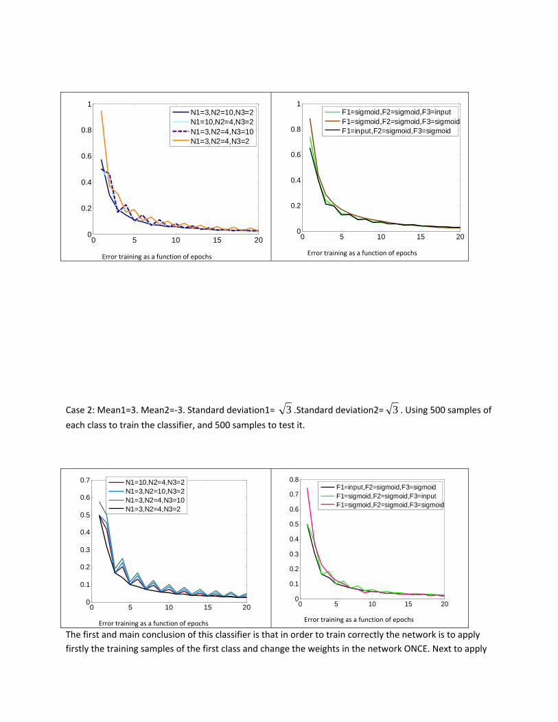
Case 2: Mean1=3. Mean2=‐3. Standard deviation1= 3 .Standard deviation2= 3 . Using 500 samples of
each class to train the classifier, and 500 samples to test it.
The first and main conclusion of this classifier is that in order to train correctly the network is to apply firstly the training samples of the first class and change the weights in the network ONCE. Next to apply
0 5 10 15 200
0.2
0.4
0.6
0.8
1
N1=3,N2=10,N3=2N1=10,N2=4,N3=2N1=3,N2=4,N3=10N1=3,N2=4,N3=2
Error training as a function of epochs
0 5 10 15 200
0.2
0.4
0.6
0.8
1
F1=sigmoid,F2=sigmoid,F3=inputF1=sigmoid,F2=sigmoid,F3=sigmoidF1=input,F2=sigmoid,F3=sigmoid
Error training as a function of epochs
0 5 10 15 200
0.1
0.2
0.3
0.4
0.5
0.6
0.7
N1=10,N2=4,N3=2N1=3,N2=10,N3=2N1=3,N2=4,N3=10N1=3,N2=4,N3=2
Error training as a function of epochs
0 5 10 15 200
0.1
0.2
0.3
0.4
0.5
0.6
0.7
0.8
F1=input,F2=sigmoid,F3=sigmoidF1=sigmoid,F2=sigmoid,F3=inputF1=sigmoid,F2=sigmoid,F3=sigmoid
Error training as a function of epochs
the training samples of the second class. Once we have all the classes trained once, we return to the first one again and repeat the process until the stop criterion is achieved.
Above are shown the performance of the classifier in terms of the training error for different network configurations. We define N1= number of nodes in the first layer, N2 = number of nodes in the hidden layer, N3 = number of nodes in the last layer. In all the simulations we have taken half of samples as training samples and the other half for testing purposes.
So we see that for small number of epochs the error training is small when use more nodes, regardless at which layer they are. This is due to the larger number of weights (order of freedom) that it used. When different types of functions where considered we observed that if we use sigmoids in all the nodes there are no oscillations as the number of epochs increases, but the error is larger for small epoch values.
Another interesting property is that no matter the combinations of functions we use, the convergence error is still the same in all methods for each particular case.
2.2 Support Vector Machine
Background review: As a machine learning tool, SVM is about learning structure from data. In our case we want to learn the mapping: YX a , where Xx ∈ is some object and Yy ∈ is a class label. The
method to do this is to find a function which minimizes an objective, like: Training Error + Complexity Term. For this experiment we chose the following formulation:
∑ ∑−ΦΦ=ji i
iijiji yxxD,
)()(21)(min ααααα where )()()( jijiji xxyyxx =ΦΦ
Subject to these constraints: Ci ≤≤ α0 k∀ and ∑ =i
ii y 0α
This is solved via matlab calling the quadprog function, which solves quadratic programming problems.
Then we define: ∑=i
iii xyw α , and IIII wxyb −−= )1( ε where }{max iiaI α= .
Note that all data points having iα >0 will be the support vectors. Then the classify rule goes like this:
).(),,( bxwsignbwxf −=
Experiment Results
Similar to project 1 we generated a pseudo‐random sample points, which generate normally distributed random numbers N(µ,σ) and separated into two different labeled classes. As in the neural network classifier we show the performance of this classifier by showing its error training and error test. In this case we have carried out two experiments: one set with data points more compacted and the other with
a more “relaxed” location, and we change different simulation parameter to examine the behavior of our classifier.
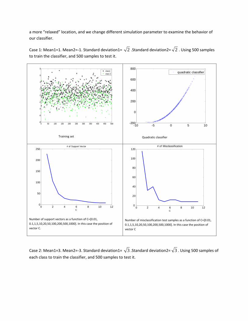
Case 1: Mean1=1. Mean2=‐1. Standard deviation1= 2 .Standard deviation2= 2 . Using 500 samples to train the classifier, and 500 samples to test it.
0 50 100 150 200 250 300 350 400 450 500-8
-6
-4
-2
0
2
4
6
8
class1class 2
Training set
-10 -5 0 5 10-200
0
200
400
600
800
quadratic classifier
Quadratic classifier
0 2 4 6 8 10 120
50
100
150
200
250# of Support Vector
C
Number of support vectors as a function of C=[0.01, 0.1,1,5,10,20,50,100,200,500,1000]. In this case the position of vector C.
0 2 4 6 8 10 120
20
40
60
80
100
120# of Misclassification
C
Number of misclassification test samples as a function of C=[0.01, 0.1,1,5,10,20,50,100,200,500,1000]. In this case the position of vector C
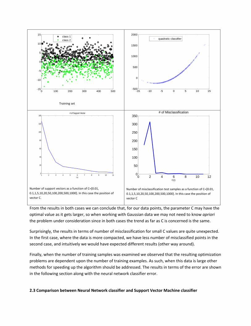
Case 2: Mean1=3. Mean2=‐3. Standard deviation1= 3 .Standard deviation2= 3 . Using 500 samples of
each class to train the classifier, and 500 samples to test it.
0 100 200 300 400 500-15
-10
-5
0
5
10
15
class 1class 2
Training set
-15 -10 -5 0 5 10 15-500
0
500
1000
1500
2000
quadratic classifier
1 2 3 4 5 6 7 8 9 10 110
20
40
60
80
100
120
140# of Support Vector
C(i)
Number of support vectors as a function of C=[0.01, 0.1,1,5,10,20,50,100,200,500,1000]. In this case the position of vector C.
0 2 4 6 8 10 120
50
100
150
200
250
300
350# of Misclassification
C(i)
Number of misclassification test samples as a function of C=[0.01, 0.1,1,5,10,20,50,100,200,500,1000]. In this case the position of vector C
From the results in both cases we can conclude that, for our data points, the parameter C may have the optimal value as it gets larger, so when working with Gaussian data we may not need to know apriori the problem under consideration since in both cases the trend as far as C is concerned is the same.
Surprisingly, the results in terms of number of misclassification for small C values are quite unexpected. In the first case, where the data is more compacted, we have less number of misclassified points in the second case, and intuitively we would have expected different results (other way around).
Finally, when the number of training samples was examined we observed that the resulting optimization problems are dependent upon the number of training examples. As such, when this data is large other methods for speeding up the algorithm should be addressed. The results in terms of the error are shown in the following section along with the neural network classifier error.
2.3 Comparison between Neural Network classifier and Support Vector Machine classifier

In this section we briefly discuss the performance of both the neural network classifier and the SVM classifier in terms of the test error performance. Note though, that there is no perfect comparison between these methods, here we have focused on the error performance for different situations.
P(e) Neural Network Classifier SVM Classifier Case 1 0.6060
2 epochs 0.2393 8 epochs
0.2343 To infinity
0.4764 C=0.1
0.2065 C=10
0.1763 C= infinity
Case 2 0.5763 2 epochs
0.2532 8 epochs
0.2123 To infinity
0.5432 C=0.1
0.2125 C=10s
0.1664 C= infinity
For our set‐up we obtained the results shown above, where the SVM classifier performed better since it achieves smaller error values for some C’s than the convergence error (best case) of the neural network classifier. Also the error is smaller for the second case where the data is more separable.
The figures below show the performance of both classifiers in terms of error training.
0 5 10 15 200
0.2
0.4
0.6
0.8
1
Training error for the Neural Network Classifier as a function of epochs.
0 2 4 6 8 10 120
0.1
0.2
0.3
0.4
0.5Training Error
C(i)
Training error for the Support Vector Machine Classifier as a function of C=[0.01, 0.1,1,5,10,20,50,100,200,500, 1000]. In this case the position of vector C.
However, in terms of computational time, the neural network classifier performed much faster, and this is something to take into account for large data sets.
Problem 3
3.1 Parzen Windows classifier
Background review: Parzen window approach consists of estimating densities by temporarily assuming
that the region nR is a d‐dimensional hypercube. If nh is the length of an edge of that hypercube, then
its volume is given by dnn hV = .
In the simplest case, if the window function is a unit function. Then, the estimate of the density at x is given as:
∑=
⎟⎟⎠
⎞⎜⎜⎝
⎛ −=
n
i n
i
nn h
xxVn
xp1
11)( φ
And by unit function we mean:
⎩⎨⎧ −≤
=otherwise
djvv j
,0,...,1;2/1||,1
)(φ
)(xpn expression suggests a general approach to estimating density functions. For Parzen window
method, the choice of the hypercube volume has an important effect on )(xpn . If nV is too large, the
estimate will suffer from too little resolution; if nV is too small, the estimate will suffer from too much
statistical variability. With a limited number of samples, the best we can do is to seek some acceptable
compromise. However, with an unlimited number of samples, it is possible to let nV slowly approach
zero as n increases and have )(xpn converge to the unknown density ).(xp
Parzen Window design: Due to the Gaussian nature of our test and training data, [1] suggests the following function:
⎟⎟⎠
⎞⎜⎜⎝
⎛ −=
2exp
21)(
2vvπ
φ
Using n
hhn1= , where 1h is a design parameter we can obtain the estimate of the density expressed as
follows:
( ) ( )( )∑=
−−−∝n
ini
Tinn hxxxx
nhnxp
1
2
1
)2/()(exp/
11)(
Experiment Results
As required in this project, and similar to project 1 we used a set of sample data, half of which is used as training data and the other half is used as test data. To see the performance of our classifier we have carried out several simulations using different lengths of data samples and different hypercube sizes.
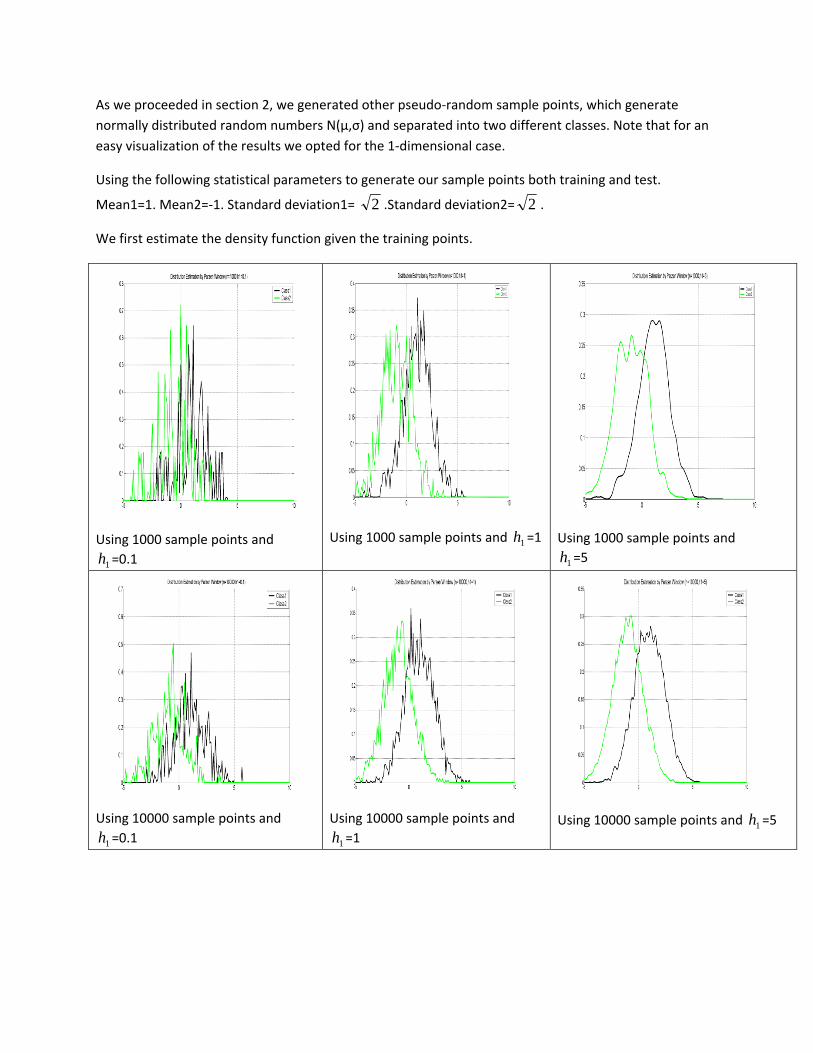
As we proceeded in section 2, we generated other pseudo‐random sample points, which generate normally distributed random numbers N(µ,σ) and separated into two different classes. Note that for an easy visualization of the results we opted for the 1‐dimensional case.
Using the following statistical parameters to generate our sample points both training and test.
Mean1=1. Mean2=‐1. Standard deviation1= 2 .Standard deviation2= 2 .
We first estimate the density function given the training points.
Using 1000 sample points and
1h =0.1
Using 1000 sample points and 1h =1
Using 1000 sample points and
1h =5
Using 10000 sample points and
1h =0.1
Using 10000 sample points and
1h =1
Using 10000 sample points and 1h =5
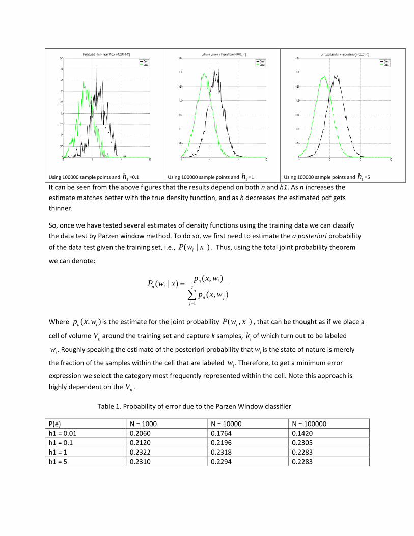
Using 100000 sample points and 1h =0.1 Using 100000 sample points and 1h =1 Using 100000 sample points and 1h =5
It can be seen from the above figures that the results depend on both n and h1. As n increases the estimate matches better with the true density function, and as h decreases the estimated pdf gets thinner.
So, once we have tested several estimates of density functions using the training data we can classify the data test by Parzen window method. To do so, we first need to estimate the a posteriori probability
of the data test given the training set, i.e., )|( xwP i . Thus, using the total joint probability theorem
we can denote:
∑=
= c
jjn
inin
wxp
wxpxwP
1
),(
),()|(
Where ),( in wxp is the estimate for the joint probability ),( xwP i , that can be thought as if we place a
cell of volume nV around the training set and capture k samples, ik of which turn out to be labeled
.iw Roughly speaking the estimate of the posteriori probability that iw is the state of nature is merely
the fraction of the samples within the cell that are labeled .iw Therefore, to get a minimum error
expression we select the category most frequently represented within the cell. Note this approach is
highly dependent on the nV .
Table 1. Probability of error due to the Parzen Window classifier
P(e) N = 1000 N = 10000 N = 100000 h1 = 0.01 0.2060 0.1764 0.1420 h1 = 0.1 0.2120 0.2196 0.2305 h1 = 1 0.2322 0.2318 0.2283 h1 = 5 0.2310 0.2294 0.2283
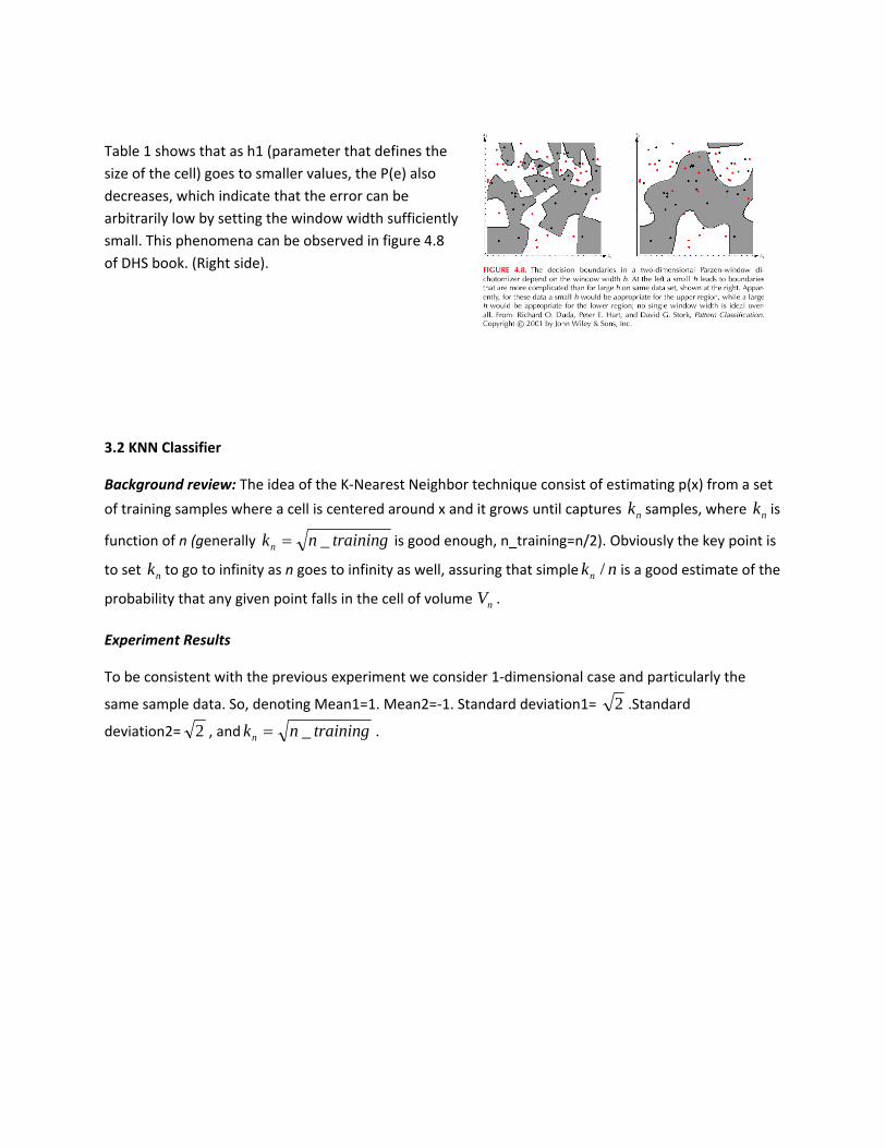
Table 1 shows that as h1 (parameter that defines the size of the cell) goes to smaller values, the P(e) also decreases, which indicate that the error can be arbitrarily low by setting the window width sufficiently small. This phenomena can be observed in figure 4.8 of DHS book. (Right side).
3.2 KNN Classifier
Background review: The idea of the K‐Nearest Neighbor technique consist of estimating p(x) from a set
of training samples where a cell is centered around x and it grows until captures nk samples, where nk is
function of n (generally trainingnkn _= is good enough, n_training=n/2). Obviously the key point is
to set nk to go to infinity as n goes to infinity as well, assuring that simple nkn / is a good estimate of the
probability that any given point falls in the cell of volume nV .
Experiment Results
To be consistent with the previous experiment we consider 1‐dimensional case and particularly the
same sample data. So, denoting Mean1=1. Mean2=‐1. Standard deviation1= 2 .Standard
deviation2= 2 , and trainingnkn _= .
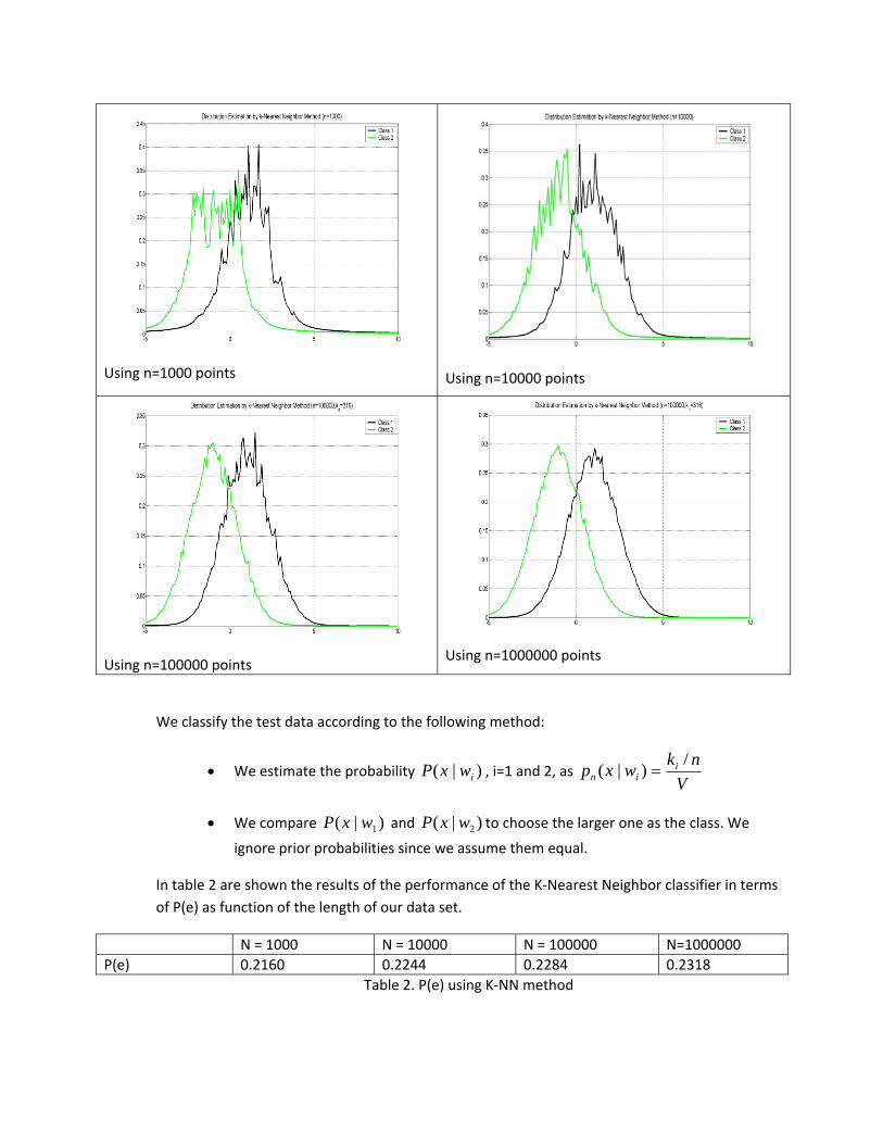
Using n=1000 points Using n=10000 points
Using n=100000 points Using n=1000000 points
We classify the test data according to the following method:
• We estimate the probability )|( iwxP , i=1 and 2, as V
nkwxp iin
/)|( =
• We compare )|( 1wxP and )|( 2wxP to choose the larger one as the class. We
ignore prior probabilities since we assume them equal.
In table 2 are shown the results of the performance of the K‐Nearest Neighbor classifier in terms of P(e) as function of the length of our data set.
N = 1000 N = 10000 N = 100000 N=1000000 P(e) 0.2160 0.2244 0.2284 0.2318 Table 2. P(e) using K‐NN method

3.3 NN Classifier
This is a particular case of the K‐Nearest Neighbor method, where the class is predicted to be the class of the closest training sample, i.e. the algorithm just looks at one nearby neighbor. If the number of samples is not large it makes a good sense to use, instead of the k‐nearest neighbor, the single nearest neighbor
Again, defining Mean1=1. Mean2=‐1. Standard deviation1= 2 .Standard deviation2= 2 , and 1=nk .
Using n=1000 points
Using n=10000 points
Using n=100000 points
Using n=1000000 points
In table 2 are shown the results of the performance of the K‐Nearest Neighbor classifier in terms of P(e) as function of the length of our data set.
N = 1000 N = 10000 N = 100000 N=1000000 P(e) 0.2070 0.1837 0.1823 0.1688
Table 3. P(e) using NN method
Comparison of all three classifiers
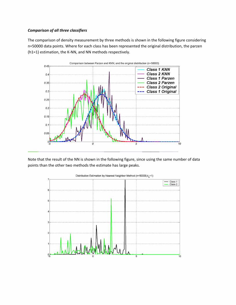
The comparison of density measurement by three methods is shown in the following figure considering n=50000 data points. Where for each class has been represented the original distribution, the parzen (h1=1) estimation, the K‐NN, and NN methods respectively.
Note that the result of the NN is shown in the following figure, since using the same number of data points than the other two methods the estimate has large peaks.

The comparison of the performance of all three methods in terms of P(e) is provided in the following table. In the cases we use have of the total data as a training set and the other half as a test set.
P(e) N=1000 N=10000 N=100000 N=1000000 Parzen Window ( 1.01 =h )
0.2120 0.2196 0.2305 0.2331
Parzen Window ( 11 =h )
0.2322 0.2318 0.2283 0.2284
KNN ( trainingnkn _= )
0.2160 0.2244 0.2284 0.2318
NN ( 1=nk ) 0.2170 0.2237 0.2193 0.2188
Table4. P(e) comparison for Parzen, KNN, and NN methods
It can be seen that when the sample data are small, the error results fluctuate, but as N increases the Parzen and KNN methods the classification errors from these methods are getting closer and eventually converge to the same error statistics. Nearest Neighbor has, for this data, a smaller error probability than the other two methods, this leads to the following statement: among the k‐nearest neighbor, the single neighbor rule is admissible. In fact, in [1] the authors show that under certain conditions 1‐NN achieves a lower error rate than k‐NN. However, the usage of large values of k in the k‐Nearest Neighbor yields to smoother decision regions. In general, it is better to use K>1 but not too large since it could lead to over‐smoothed boundaries.
[1] T.M. Cover, and P.E. Hart, “Nearest Neighbor Pattern Classification”, IEEE Transactions of Information theory, vol. 17, no. 1, January 1967.
APPENDIX(Source Code)
P.1 paramet.m
% Hw 2 p1 Parametric Method
clear all;close all;
% sample points
n1=200;
n2=200;
% 1‐dim
mean_x1 = 1;
var_x1 = 2;
mean_x2 = ‐1;
var_x2 = 2;
x1 = mean_x1 + sqrt(var_x1)*randn(1,n1);
x2 = mean_x2 + sqrt(var_x2)*randn(1,n2);
% 2‐dim
Mean1 = [ 1 1]';
Mean2 = [ ‐3 1]';
std1 = [8 1; 1 1];
std2 = [3 1; 1 1];
data_class1 = mvnrnd(Mean1,std1,n1);
data_class2 = mvnrnd(Mean2,std2,n2);

plot(data_class1(:,1),data_class1(:,2),'ko');hold on;
plot(data_class2(:,1),data_class2(:,2),'g+');
x1=data_class1;
x2=data_class2;
figure,
mhu_1=(1/n1)*(sum(x1));
mhu_2=(1/n2)*(sum(x2));
bet_scatter= (mhu_1‐mhu_2);
% S_B = eye(f,c);
S_W1 = size(x1,1)*cov(x1);
S_W2 = size(x2,1)*cov(x2);
S_W = S_W1+S_W2;
[f,c]=size(S_W);
%S_W=eye(f,c);
w_opt=S_W\bet_scatter';
% Projections
y1 = x1*w_opt;
y2 = x2*w_opt;
bin = 0.1;
x = ‐25:bin:25;
xa = 1:length(y1);
xb=1:length(y2);
plot(xa,y1,'k',xb,y2,'g');figure,
hist(x1,x);
figure,
hist(x2,x);
%plot(y1,'k');hold on;
%plot(y2,'g');hold off;
P2 Neural Network
% performs backpropagation algorithm
close all;clear all;
N1 = 6;N2 = 12;N3 = 3;
iter = 50;
iter_test = 50;
Target = zeros(1,N3);
% initialize weights
W_hid_in = rand(1,N1);
W_hid_out = rand(1,N2);
error_epoch = zeros(1,iter);
error_epoch_test = zeros(1,iter_test);
Mean1 = 1;
Mean2 = ‐1;
std1 = 2;
std2 = 2;
data_class1 = Mean1 + std1*randn(1,N1);
data_class2 = Mean2 + std2*randn(1,N1);
for k=1:iter
if (mod(k,2)==0)
training_data = data_class1;
else
training_data = data_class2;
epoch=k,
end
for i=1:N1
sig_output(i) = training_data(i);
end
% training the neural network step
% outputs
for n=1:N3
in_last(n)=0;
for j=1:N2
input_hid(j)=0;
for i=1:N1
input_hid(j) = input_hid(j)+W_hid_in(i)*sig_output(i);
end
W_old_hidden(:,j) = W_hid_in';
sig_output_hid(j) = (1)/(1+exp(‐input_hid(j)));
in_last(n) = sig_output_hid(j)*W_hid_out(j)+in_last(n);
end
out(n) = (1)/(1+exp(‐in_last(n)));
W_old_output(:,n) = W_hid_out';
end
lear_rate = 0.25;
% backpropagation step
% calculate errors of output neurons
for i=1:N3
delta(i) = out(i)*(1‐out(i))*(Target(i)‐out(i));
end
% Change output layer weights
for i=1:N2
for j=1:N3
W_new_output(i,j) = W_old_output(i,j)+lear_rate*delta(j)*sig_output_hid(i);
end
end

% back‐propagate
for i=1:N2
ssuumm=0;
for j=1:N3
ssuumm = delta(j)*W_new_output(i,j)+ssuumm;
end
delta_hid(i) = sig_output_hid(i)*(1‐sig_output_hid(i))*ssuumm;
end
% change hidden layer weights
for i=1:N1
for j=1:N2
W_new_hidden(i,j) = W_old_hidden(i,j)+lear_rate*delta_hid(j)*training_data(i);
end
end
W_old_output = W_new_output;
W_old_hidden = W_new_hidden;
% forward pass with the new weights
for i=1:N1
sig_output(i) = training_data(i);
end
% outputs
for n=1:N3
in_last(n) = 0;
W_hid_out = W_new_output(:,n)';
for j=1:N2
input_hid(j) = 0;
W_hid_in = W_new_hidden(:,j)';
for i=1:N1
input_hid(j) = input_hid(j)+W_hid_in(i)*sig_output(i);
end
sig_output_hid(j) = (1)/(1+exp(‐input_hid(j)));
in_last(n) = sig_output_hid(j)*W_hid_out(j)+in_last(n);
end
output(n,k) = (1)/(1+exp(‐in_last(n)));
error(k) = abs(Target(n)‐output(n,k));
end
error_epoch(k) = (error_epoch(k)+error(k))/k;
end
x=1:iter;
plot(x,error_epoch,'k'); hold on;
y=zeros(1,iter_test);
%% Testing...
for k=1:iter_test
data_class1 = Mean1 + std1*randn(1,N1);
data_class2 = Mean2 + std2*randn(1,N1);
% Generating the test data
p=randperm(2);
if (p(1)==1)
training_data = data_class1;
else
training_data = data_class1;
end
epoch=k,
for i=1:N1
sig_output(i) = training_data(i);
end
% outputs
for n=1:N3
in_last(n) = 0;
for j=1:N2
input_hid(j) = 0;
for i=1:N1
input_hid(j) = input_hid(j)+W_hid_in(i)*sig_output(i);
end
sig_output_hid(j) = (1)/(1+exp(‐input_hid(j)));
in_last(n) = sig_output_hid(j)*W_hid_out(j)+in_last(n);
end
outpu_test(n,k) = (1)/(1+exp(‐in_last(n)));
error_test(k) = abs(Target(n)‐outpu_test(n,k));
end
error_epoch_test(k) = (error_epoch_test(k)+error_test(k))/k;
y(k)=(y(k)+1)/k
end
x=1:iter_test;
%plot(x,y,'b'); hold on;
plot(x,error_epoch_test,'g'); hold off;
SVM
Clear all; close all;
nsample = 100;
Mean1 = 1;
Mean2 = ‐1;

std1 = 2;
std2 = 2;
data_class1 = Mean1 + std1*randn(1,nsample/2);
data_class2 = Mean2 + std2*randn(1,nsample/2);
X(1:nsample/2) = data_class1;
X(nsample/2+1:nsample) = data_class2;
X = sort(X);
plot(data_class1,'ko');hold on;
plot(data_class2,'g+');
p = randperm(nsample);
Y(p(1:nsample/2)) = ‐1;
Y(p(nsample/2+1:nsample)) = 1;
% the trade‐off weights
C = [0.1, 1, 5, 10, 20, 50, 100, 200, 500, 1000, 2000, 5000, 10000, 100000];
Margin = []; % margin; initialized as null
nSV = []; % number of support vector;
nMis = []; % number of misclassification;
Err = []; % training errors;
X,Y,
for n = 1 : max(size(C)),
% construct Hessian matrix;
H = zeros(nsample, nsample);
for i = 1 : nsample,
for j = 1 : nsample,
H(i,j) = X(i)*X(j)*Y(i)*Y(j);
end
end
H = H+1e‐10*eye(size(H));
F = ‐ones(nsample,1); % F' * Alpha corresponds to sigma_i(Alpha_i) in object function
% set up equality constraints
A = Y'; % corresponds to sigma_i(Alpha_i * Y_i) = 0
b = 0;
% set up upper and lower bounds for alpha: LB <= Alpha <= UB
UB = zeros(nsample,1);
LB = C(n)*ones(nsample,1);
% starting point of alpha
Alpha0 = zeros(nsample, 1);
% optimizing alpha with quadratic programming
[Alpha] = quadprog(H, F, [], [], A, b, LB, UB, Alpha0),
% tolerance for support vector detection; we will ignore the alphas less than tol
tol = 0.0001;
% calculate weight
w = 0;
for i = 1 : nsample,
w = w + Alpha(i) * Y(i) * X(i);
end
% calculate bias
bias = 0;
b1 = 0;
b2 = 0;
for i = 1 : nsample,
if (Alpha(i) > tol & Alpha(i) < C(n) ‐ tol),
b1 = b1 + X(i) * w ‐ Y(i);
b2 = b2 ‐ 1;
end
end
if b2 ~= 0,
bias = b1 / b2;
else % unlikely
b1 = 0;
for i = 1 : nsample,
if Alpha(i) < tol,
b1 = b1 + X(i) * w ‐ Y(i);
b2 = b2 ‐ 1;
end
end
if b2 ~= 0,
bias = b1 / b2;
else % even unlikelier
b1 = 0;
for i = 1 : nsample,
b1 = b1 + X(i) * w ‐ Y(i);
b2 = b2 ‐ 1;
end
if b2 ~= 0,
bias = b1 / b2;
end
end
end
% margin = 2 / ||w||
Margin = [Margin, 2 / abs(w)];
% number of support vectors
nSV = [nSV, size(find(Alpha > tol), 1)];
% calculate # of misclassification and training error

m = 0;
e = 0;
for i = 1 : nsample,
predict = w * X(i) + bias; % Y = w * X + b
if predict >= 0 & Y(i) < 0,
m = m + 1;
end
if predict < 0 & Y(i) >= 0,
m = m + 1;
end
if Alpha(i) > tol,
e = e + 1 ‐ predict * Y(i);
end
end
nMis = [nMis, m],
Err = [Err, e],
end
Z = zeros(size(C));
for i = 1 : size(C, 2)
Z(i) = i;
end
figure
plot(Z, Margin);
title('Margin');
xlabel('C(i)');
figure
plot(Z, Err);
title('Training Error');
xlabel('C(i)');
figure
plot(Z, nMis);
title('# of Misclassification');
xlabel('C(i)');
figure
plot(Z, nSV);
title('# of Support Vector');
xlabel('C(i)');
P3 Parzen Window
clear all;
close all;
% initialize random number generator
randn('state',100)
n = 5000;
n_train = n/2;
n_test = n/2;
% Data set 1: x1 with distribution N(a,b) (mean=a, var=b)
mean_x1 = 1;
var_x1 = 2;
x1 = mean_x1 + sqrt(var_x1)*randn(1,n);
mean(x1)
var(x1)
x1_train = x1(1:n_train);
x1_test = x1(n_train+1:end);
% Data set 2: x2 with distribution N(a,b) (mean=a, var=b)
mean_x2 = ‐1;
var_x2 = 2;
x2 = mean_x2 + sqrt(var_x2)*randn(1,n);
mean(x2)
var(x2)
x2_train = x2(1:n_train);
x2_test = x2(n_train+1:end);
bin = 0.1;
x = ‐5:bin:10;
L_x = length(x);
figure
hist(x1,x)
dis_1 = hist(x1,x);
%normalize the value of distribution to (0,1)
y_1 = dis_1/(n*bin);
figure
hist(x2,x)
dis_2 = hist(x2,x);
%normalize the distribution to (0,1)
y_2 = dis_2/(n*bin);
figure
plot(x,y_1,'b‐',x,y_2,'r.‐')
title('Distribution of Class 1 and Class 2')
grid on
legend('Distribution of class1','Distribution of class2')
% 1‐dimentional
d = 1; % dimention
%setting h1
h1 = 1;
hn = h1/sqrt(n_train);
Vn = hn^d;
Q1 = zeros(1,n_train);
prob1_train = zeros(1,L_x);
Q2 = zeros(1,n_train);
prob2_train = zeros(1,L_x);
% window function
for i = 1:L_x
for j = 1:n_train
Q1(j) = 1/(sqrt(2*pi))*exp(‐(x(i) ‐ x1_train(j))^2/(2*hn^2));
Q2(j) = 1/(sqrt(2*pi))*exp(‐(x(i) ‐ x2_train(j))^2/(2*hn^2));
prob1_train(i) = prob1_train(i) + 1/n_train*1/Vn*Q1(j);
prob2_train(i) = prob2_train(i) + 1/n_train*1/Vn*Q2(j);
end
end
figure
plot(x,prob1_train,'k.‐', x,prob2_train,'g.‐')
grid on
hold on
title('Distributioin Estimation by Parzen Window (n=4000,h1=1)')
legend('Class1','Class2')
%errors by Parzen window method
error1_parzen = 0;
error2_parzen = 0;
for i = 1:n_test
% find(X) locates all nonzero elements of array X, and returns the indices of those elements
j1_parzen = find(abs(x‐x1_test(i)) <= 0.1);
if (prob1_train(j1_parzen) < prob2_train(j1_parzen))
error1_parzen = error1_parzen + 1;
end
j2_parzen = find(abs(x‐x2_test(i)) <= 0.1);
if(prob2_train(j2_parzen) < prob1_train(j2_parzen))
error2_parzen = error2_parzen + 1;
end
end
error_parzen_total = error1_parzen + error2_parzen
error_parzen_prob = error_parzen_total/(2*n_test)
KNN
clear all
close all
% Using the normally distributed data from MATLBA random number generator
% for the data used in this problem.
%sample data
n = 5000;
n_train = n/2;
n_test = n/2;
% Data set 1: x1 with distribution N(a,b) (mean=a, var=b)
mean_x1 = 1;
var_x1 = 2;
x1 = mean_x1 + sqrt(var_x1)*randn(1,n);
mean(x1)
var(x1)
x1_train = x1(1:n_train);
x1_test = x1(n_train+1:end);
% Data set 2: x2 with distribution N(a,b) (mean=a, var=b)
mean_x2 = ‐1;
var_x2 = 2;
x2 = mean_x2 + sqrt(var_x2)*randn(1,n);
mean(x2)
var(x2)
x2_train = x2(1:n_train);
x2_test = x2(n_train+1:end);
bin = 0.1;
x = ‐5:bin:10;
L_x = length(x);
figure
hist(x1,x)
dis_1 = hist(x1,x);
%normalize the value of distribution to (0,1)
y_1 = dis_1/(n*bin);
figure
hist(x2,x)
dis_2 = hist(x2,x);
%normalize the distribution to (0,1)
y_2 = dis_2/(n*bin);
figure
plot(x,y_1,'b‐',x,y_2,'r.‐')
title('Distribution of Class 1 and Class 2')
grid on
legend('Distribution of class1','Distribution of class2')
% function of kn (KNN)
kn = round(sqrt(n_train));
% function of kn (NN)
kn = 1;
prob1_nn = zeros(1,L_x);

prob2_nn = zeros(1,L_x);
for i = 1:L_x
index_sort1 = sort(abs(x1_train ‐ x(i)));
Vn1 = 2 * index_sort1(kn);
index_sort2 = sort(abs(x2_train ‐ x(i)));
Vn2 = 2 * index_sort2(kn);
if (Vn1 > 0)
prob1_nn(i) = kn/n_train/Vn1;
end
if(Vn2 > 0)
prob2_nn(i) = kn/n_train/Vn2;
end
if (prob1_nn(i)>10)
prob1_nn(i)=0;
end
if (prob2_nn(i)>10)
prob2_nn(i)=0;
end
end
figure
plot(x,prob1_nn,'k.‐',x,prob2_nn,'g.‐')
grid on
title('Distribution Estimation by k‐Nearest Neighbor Method (n=100000,k_n=316)')
legend('Class 1','Class 2')
error_nn_total = 0;
error1_nn = 0;
error2_nn = 0;
for i = 1:n_test
j1_nn = find(abs(x‐x1_test(i)) <=0.1);
if (prob1_nn(j1_nn) < prob2_nn(j1_nn))
error1_nn = error1_nn +1;
end
j2_nn = find (abs(x‐x2_test(i))<=0.1);
if(prob2_nn(j2_nn) < prob1_nn(j2_nn))
error2_nn = error2_nn +1;
end
end
error_nn_total = (error1_nn + error2_nn)/2/n_test