Homework in Monetary Economics:

In�ation, Home Production, and the

Production of Homes�

S. Bora¼gan Aruobay

University of Maryland

Morris A. DavisUniversity of Wisconsin �Madison

Randall WrightUniversity of Wisconsin �Madison, FRB Minneapolis, FRB Chicago and NBER

July 14, 2014

Abstract

We introduce household production and the production of houses (construc-tion) into a monetary model. Theory predicts in�ation, as a tax on marketactivity, encourages substitution into household production and hence invest-ment in housing. In the model, the stock and appropriately-de�ated price ofhousing increase with in�ation or nominal interest rates. We document thisin data for the U.S. and other countries. A calibrated model accounts for upto 52% (87%) of the relationship between interest rates and housing wealthde�ated by nominal output (by the money supply). It also implies the cost ofin�ation is higher than in models without home production.

�We thank many friends and colleagues for helpful input, especially Christophe André, Je¤Campbell, Larry Christiano, Marcello Veracierto, Yu Zhu, and Gwen Eudey. Aruoba and Wrightalso thank the NSF, Davis and Wright thank the Lincoln Institute of Land Policy, and Wrightthanks the Ray Zemon Chair in Liquid Assets at the Wisconsin School of Business for researchsupport. The usual disclaimer applies.

yCorresponding author. email: aruoba@econ.umd.edu; phone: 301-405-3508.

1 Introduction

This paper reports the results of our research in monetary economics applied to

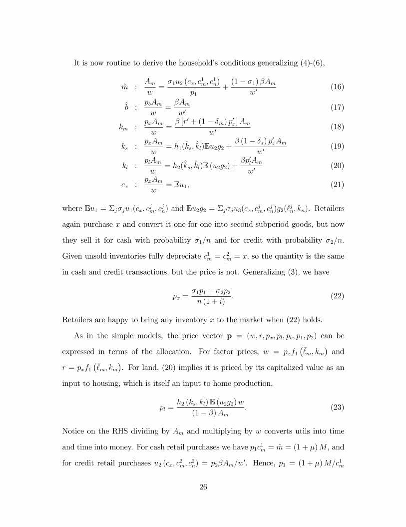
the housing market, including some novel data analysis, a new theory, and a cali-

bration exercise. In fact, the theory is not so much new as a combination of three

existing literatures. The basic framework follows the now standard approach to the

microfoundations of monetary theory, sometimes called New Monetarist Economics,

that provides benchmark models of money, credit, banking, over-the-counter �nan-

cial markets and related phenomena. Into this we introduce household production,

since we believe it is best to think about home capital (residential structures and

consumer durables) as a factor of production, parallel to the way economists think

about market capital (nonresidential structures and producer durables). Then we

import features from the literature that studies the production of houses, because

we are interested in the supply side as well as the demand side of housing markets.

Although each of these elements has been studied extensively, they have not been

previously interrelated.1

As one motivation for the project, consider the often-heard view that there is

a connection between monetary policy and housing markets. While there may be

several ways to think about such a connection, one is the common notion that hous-

ing is a good hedge against in�ation. That notion is vague, but the interpretation

adopted here is this: the value of housing wealth increases when in�ation is higher.

By a hedge, we do not mean that one can use housing to avoid in�ation risk, al-

though that may also be interesting; the idea is rather that having more housing

1Since we are combining several di¤erent literatures we cannot list every relevant paper. Onthe microfoundations of monetary economics, we discuss below the work on which we build directly,but see Williamson and Wright (2010a,b) and Nosal and Rocheteau (2011) for recent surveys. Onhome production, there are surveys by Greenwood et al. (1995) and Gronau (1997), although therehas been a lot of work since then, as discussed below. We also review some housing research, butan example of what we have in mind is Davis and Heathcote (2005).

1

allows one to partially avoid some of the e¤ects of anticipated in�ation. A goal

of the paper is to make this precise, but to get some rough intuition, consider the

so-called Tobin e¤ect that says that in�ation makes agents want to substitute out

of cash and into capital. Our e¤ect is similar, except we focus on household instead

of market capital. To put it di¤erently, in most monetary models, in�ation makes

agents want to substitute out of consumption and into leisure; in our model they

substitute into household production.

While part of the objective is methodological � integrating approaches from

di¤erent literatures into a framework that can be useful in a variety of applications

�we also want to discuss some substantive issues. First we check the facts, using

various data sources, for the U.S. and other countries. We construct from di¤erent

sources several measures of housing wealth, scaled by either nominal output or by

the money supply (one has to scale by something, obviously, to control for purely

nominal e¤ects). We then show these series for housing wealth are positively related

to nominal interest and in�ation rates. Although one may be able to think of

di¤erent explanations for this evidence, we pursue the idea that in�ation is a tax on

market activity. This is surely relevant in high-in�ation, cash-intensive economies,

but it is also interesting to explore the channel for the U.S. In�ation and nominal

rates have been low here for a while, but the 1970s runup and subsequent decline

provide plenty of variation in the data. And as regards cash intensiveness, note that

in�ation impacts not only currency but many other assets.2

By way of example, higher in�ation or nominal interest rates provide an incentive

to go out for dinner less and eat more meals at home, as long as going out is

relatively cash intensive. Now, not all market activity uses cash, but it uses cash

2It obviously a¤ects demand deposits, especially when interest payments on these are quitelow, but more generally in�ation a¤ects the returns to all liquid assets. See Lester et al. (2012) andVenkateswaran and Wright (2013) for models making this point theoretically and quantitatively.

2

more than household activity, since goods like home-cooked meals are not even

traded, let alone traded using currency. Thus, in�ation increases the demand for

home-production inputs, which raises the value of housing wealth, through prices,

and through quantities as construction catches up. Quite generally, as long as high

in�ation or nominal interest rates discourage market activity, and thus encourage

household activity, they should a¤ect the demand for housing.

Another reason for integrating these literatures is the following. A classic ques-

tions in economics asks about the e¤ect of in�ation on welfare. One should think

that the answer will be a¤ected by incorporating home production, given that much

previous work has shown that adding it to otherwise standard models makes a sig-

ni�cant di¤erence for various other quantitative questions.3 Typically, the main

impact of incorporating home production is that it changes the amount by which

agents respond to changes in policy and other forcing variables. In the standard

macro model, agents can substitute between leisure and labor and between con-

sumption and investment. In models with home production, they can substitute

between leisure and working in the market or working at home, and between con-

sumption and investment in market capital or home capital. It has been shown that

this signi�cantly a¤ects the quantitative impact of �scal policy (by several of the

papers in fn. 3); we want to know how it a¤ects the impact of monetary policy.

To implement these ideas, the model of money and capital in Aruoba et al. (2011)

is generalized to include home production and the production of homes (construc-

3Benhabib et al. (1991) and Greenwood and Hercowicz (1991) put ideas about home productionby Becker (1965,1988) into quantitative macro models, and show they match key business-cyclemoments better than models without home production. Home production models also betterexplain consumption (Baxter and Jerrmann 1999; Baxter 2010; Aguiar and Hurst 2005,2007a),investment (Gomme et al. 2001; Fisher 1997,2007), female labor-force participation (Greenwoodet al. 2005; House et al 2008; Albanesi and Olivetti 2009), and labor supply generally (Rios-Rull1993; Rupert et al. 2000; Gomme et al. 2004; Aguiar and Hurst 2007b; Ngai and Pissarides 2008;Rogerson and Wallenius 2009). These models also give di¤erent answers to �scal policy questions(McGrattan et al. 1997; Rogerson 2009), and provide novel perspectives on development issues(Einarsson and Marquis 1997; Parente et al. 2000).

3

tion). Housing capital, like market capital, is both produced and used in production.

Following much of the work on home production, we make home capital a factor of

production instead of inserting it directly in the utility function. We stay close to

the approach in the earlier papers for the purposes of comparison, and because it

allows us to take advantage of some results in the literature, including estimates of

certain key elasticities.4

After providing analytic results that formalize the economic intuition, we cali-

brate the model, and ask how well it accounts for the empirical �ndings. The answer

is that, depending on some details, we can account for between 22% and 52% of the

relationship between interest rates and housing wealth over nominal output, and

between 78% and 87% of the relationship between interest rates and housing wealth

over the money supply. So, while the channel on which we focus is relevant, there is

room for other factors to play a role. But of course the objective is not to explain

100%; it is to show how the model can be used to measure the size of the e¤ects,

without prejudice as to whether they are big or small. We also show the welfare

cost of in�ation is higher than in similar models without home production. Again,

the goal is not to make this number big or small but to investigate the impact of

including home production.

To be clear about our methods, we generate quantitative predictions from the-

ory in the counterfactual situation where the only impulses are changes in in�ation

or nominal interest rates. This is not because we believe changes in taxes, tech-

nology, demography and other factors are irrelevant; we simply want a controlled

experiment, changing one variable holding the rest �xed. This is similar to standard

4The issue is similar to the way one handles the value of time. As discussed in the surveyscited in fn. 1, Becker�s approach assumes time does not enter utility, but consumption does, andhome work is an input into home production; by contrast, Gronau�s approach assumes agents valueleisure time per se, as well as home production. Neither is �better�but we need to pick one. As abenchmark, we assume time enters utility directly while capital does not.

4

practice in macro going back to Kydland and Prescott (1982) of asking, e.g., what a

model can explain based only on technology shocks. The paper is not about business

cycles, however. It is about medium- to long-run phenomena, because we do not

think a blip up in the CPI in one month causes people to abandon the market; we

do believe that if people face relatively permanently higher in�ation, they choose

less market and more household activity.5

In terms of other work, there is work on the relationship between in�ation and

the stock market, which is related in that stocks and housing are both alternatives

to monetary assets.6 Research analyzing housing and in�ation through e¤ects on

mortgages include Kearl (1979), Follain (1982) and Poterba (1991). This is a com-

plementary idea, and we do not want to �test� one hypothesis against the other,

given our results leave room for other theories. Brunnermeier and Juiliard (2008)

impose money illusion, confounding agents between nominal and real interest rates.

Burnside et al. (2011) also depart from standard rational expectations. While this

is �ne, we want to see how far we can go with rational agents. He et al. (2011) show

housing can bear a liquidity premium, somewhat like money, when it can be used

to secure home-equity loans. To focus on other e¤ects we abstract from this, which

seems reasonable at least before 2000, when such borrowing was less important.

Piazzesi and Schneider (2010) assume in�ation taxes the returns to �nancial

assets but not housing. This is a complementary idea, too, although their model

5It is easy to introduce shocks to technology, policy and other variables, and look at high-frequency behavior, but that would be a distraction for present purposes. More importantly, weemphasize that our theory is not inconsistent with high-frequency evidence suggesting that mone-tary shocks are associated with market expansions rather than contractions. Over longer horizons,in�ation and nominal interest rates move together, and the hypothesis that increases in these ratesare bad for market activity at low frequencies does not contradict any �ndings in, e.g., Christianoet al. (2005). For a long-run analysis �nding money growth, in�ation and nominal interest ratesmove together, and increases are bad for market activity, see Berentsen et al. (2011).

6See Geromichalos et al. (2007) for references to work on the e¤ects of in�ation on the stockmarket. See Venkateswaran and Wright (2013) for a list of empirical papers looking at the e¤ectson asset returns, more generally, as well as output and investment.

5

is very di¤erent. To highlight two di¤erences: (i) our monetary theory is built on

relatively �rm microfoundations; (ii) we incorporate home production. The �rst is

relevant because we think of the paper as a contribution to monetary economics at

least as much as a contribution to the housing literature. The second is relevant

because we also think the paper is a contribution to the home production literature,

and because this allows us to take advantage of results from that research, as men-

tioned above. To close these introductory remarks, we mention that although our

model has a frictional retail goods market, which is essential for modeling money

rigorously, housing is traded in a frictionless market. Actual markets for houses are

far from frictionless, just like actual markets for factories, workers and other inputs,

but to maintain focus, in this project, home capital and market capital are traded

in perfect markets as in standard growth theory.7

The rest of the paper is organized as follows. Section 2 discusses data. Sections

3 presents the environment. Section 4 provides simple versions of the theory that

deliver clean qualitative results. Section 5 generalizes this for quantitative analysis.

Section 6 presents the calibration exercises. Section 7 concludes.

2 Data

Here we present the case that nominal interest or in�ation rates are positively related

to the value of home capital, scaled by nominal output or by the money supply to

correct for purely nominal changes. We �rst examine the U.S., then other countries.

For the U.S. we consider several measures of home capital, by which we mean the

value (price times quantity) of the housing stock plus durable goods. We add durable

goods because we think of home capital more broadly than just housing, even if

7The growing body of research on frictional housing markets includes Wheaton (1990), Albrechtet al. (2007), Caplin and Leahy (2008), Coulson and Fisher (2009), Ngai and Tenreyro (2009),Novy-Marx (2009), Piazzesi and Schneider (2009) and Head and Lloyd-Ellis (2012).

6

housing is the lion�s share (about 3=4). At least for appliances and related consumer

durables, it seems natural to include them in home capital, parallel to the way

producer durables are included in market capital. While data sources are discussed

in the text, detailed information is given in the Appendix.

2.1 United States

Our baseline measure of housing wealth uses data from Davis and Heathcote (2007),

DH for short. A disadvantage of these data is that the sample is relatively short,

starting in 1975; an advantage is that they are quite accurate. Figure 1 shows time

series in the left column, and scatter plots as well as correlations and semi-elasticities

in the right column. The top row is home capital over nominal output versus the

nominal interest rate on T-bills. As in most work on home production, our measure

of output is GDP minus rents paid to housing services. The scatter plots show the

predicted relationships for 1975-1999 and for 2000-2009.

The �rst issue to mention is that it is apparent that something unusual �often

referred to as a bubble �was happening in the 2000s relative to the previous 25

years. This project is not about the post-2000 U.S. housing boom and bust, as

there may well have been something going on that our model is not designed to

capture, such as developments in �nancial markets, including the big increase in

home-equity lending.8 The theory presented is not a model of bubbles. While it

may be interesting in future work to extend it in that direction, it is also legitimate

to see what the theory has to say about more �normal�times. This suggests that

8As Holmstrom and Tirole (2011) put it, �In the runup to the subprime crisis, securitizationof mortgages played a major role ... by making nontradable mortgages tradable [and this] led to adramatic growth in the US volume of mortgages, home equity loans, and mortgage-backed securitiesin 2000 to 2008.�Ferguson (2008) and Reinhart and Rogo¤ (2009) characterize the situation bysaying this lead to households treating their houses as ATM machines. See Mian and Su� (2011)for more discussion of the episode, and He et al. (2011) for a model in which home-equity lendingcan generate bubbles with housing-fueled expansions and collapses.

7

it may be reasonable to stop the sample at the end of the last millennium, but we

do not want to hide anything, and so we show what happened after 2000, too.

From 1975 to 1999, home capital is clearly positively correlated with the T-bill

rate. This is also true after 2000, with a nearly-parallel shift up in the relationship.

The semi-elasticity for the 1975-1999 period is 1:1, and the correlation is 0:62. This

is the �rst key empirical �nding: nominal interest rates are positively related to the

value of home capital scaled by nominal output. One of the primary goals of the

quantitative work is to see how well theory can account for this relationship. Before

moving to models, however, we want to investigate the robustness of the facts.

The second row in Figure 1 de�ates home capital by the money supply, instead of

nominal output, where our measure of money is the M1S series that adjusts M1 for

the practice since the 1990s of sweeping checkable deposits into overnight money

market accounts (Cynamon et al. 2006). This is the second key empirical �nding:

Home capital scaled by the money supply is even more strongly positively with the

nominal rate, with a semi-elasticity around 3:7 and a correlation of 0:8.

To further check robustness, the third row in Figure 1 replaces the T-bill rate with

the AAA corporate bond rate. Before 2000, the relationship between home capital

scaled by the money supply is similar to what we found with the T-bill rate, again

with a correlation around 0:8. Although after 2000 the relationship looks di¤erent,

there is not much information in that short subsample. The last row of Figure 1

uses the in�ation rate instead of the nominal interest rate. According to the Fisher

Equation, nominal interest rates move one-to-one with in�ation, but while this is

approximately true in the longer run it is not exactly true in the shorter run. The

results are similar, although now the post 2000 data look like more like a rotation

than a shift in the relationship, but again there is not much information in that

short subsample. We slightly prefer nominal interest rates (rather than in�ation) as

8

a measure of the wedge imposed by monetary policy, because they are arguably a

better measure (than contemporaneous in�ation) of expected future in�ation, which

is what matters in the model.

To further investigate the facts, we now consider several alternative ways to

measure the value of home capital, using di¤erent data sets, some of which extend

over much longer samples. This is shown in Figure 2. The �rst row presents the

scatter between home capital scaled by nominal output, and scaled by the money

supply, against the T-bill rate, where the measure of housing wealth now uses data

from the Flow of Funds Accounts (FFA). An advantage of FFA data is that they

go back to 1952, although we think it is probably better to start in 1955, due to

possible e¤ects from the Korean War. However, a disadvantage is that FFA data

do not provide the best estimates of house values for 1975-1990, which is a key part

of the sample because it has a lot of variation in in�ation.9 Having said that, the

relationships in this data are very similar to those in Figure 1.

The second row in Figure 2 uses housing wealth data based on the replacement

cost of structures estimated by the Bureau of Economic Analysis (BEA). A disad-

vantage here is that these data do not include the value of land, which prior to

1970 was between 10 to 20 percent, and is currently about a third of housing value

(Davis and Heathcote 2007). An advantage is that they are constructed according

to well-documented methods and go back to the 1930s, although it is less clear what

to make of data that far back, where the situation is confounded by the Great De-

pression, as well as some swings in in�ation and interest rates probably having to

do with wars and price controls. In this case the regression lines come from split-

ting the sample between 1930-1954 and 1955-1999, and we use the AAA bond rate,

9This is because the housing capital gains implied by the FFA data over this period do not alignwell with capital gains computed using standard price indexes. Unlike the DH data, where capitalgains are taken directly from price indexes, for this period FFA data spline together estimates fromvarious surveys. See Davis and Heathcote (2007) for details.

9

which is readily available going back to the 1930s. For the 1955-1999 period, the

relationship in this data is even stronger than the results in Figure 1. The third

row in Figure 2 is housing wealth computed directly from the Decennial Censuses

of Housing (DCH). The advantage here is that the numbers are very accurate, and

go back to 1930, but we only get one observation every ten years, so we interpolate.

Once again, there is a very strong relationship.

The last row of Figure 2 uses Shiller�s (2005) house price index (HPI), starting

in 1955. The relationship in the right panel looks like the previous rows; the left

panel does not. But we believe there are some issues with using HPI data for our

purposes. Table 1 reconciles decade-by-decade changes in HPI and housing wealth

as follows: Column 1 reports HPI growth; Column 2 reports growth in the average

price of housing units; Column 3 reports growth in the number of units; and Column

4 reports growth in nominal GDP. The percentage change in the value of housing

is approximately Column 2 plus Column 3. Columns 1 and 2 show average prices

rise faster than the HPI in every decade. This is because Shiller�s data hold quality

constant, and the gap between Columns 1 and 2 re�ects quality improvement. Also,

these data do not track changes in the number of units, which rose rapidly over the

sample. Columns 2 and 3 show the change in housing wealth between 1950 and 2000

is 528 percent, about the same the 517 percent change in nominal GDP. The HPI

increased only 284 percent. This implies the HPI is not so useful for our purposes,

and may explain why those who focus on this data have not noticed the facts found

in all the other sources.10

10We also mention Brunnemeier and Julliard (2007), who �nd that nominal interest rates fore-cast one-period-ahead price-rent ratios. The relationship is negative and statistically signi�cant.They also �nd nominal rates forecast deviations of the price-rent ratio from trend. These �ndingsare in no way inconsistent with our results. For one thing, price-rent ratios are not the same asvalue-income ratios, which are the objects of interest here �e.g., the former can re�ect discountfactors, while the latter re�ect the desirability of housing wealth relative to one�s budget. Moreover,we are less interested in one-period-ahead forecasting than long-run relationships.

10

2.2 Other Countries

Data on housing wealth prior to 1990, and certainly prior to 1980, are virtually

nonexistent outside the U.S., but estimates of prices have been constructed for

several countries. As we said, we prefer price times quantity, but for most countries

prices are the best we can get. Figure 3 presents house prices over nominal output

versus in�ation for 16 countries.11 In�ation is used because it is harder to get

consistent measures of interest rates across countries, and now we do not distinguish

between the pre- and post-2000 data, because the boom and bust are less apparent

in these economies than in the U.S. The bottom line is that there is a positive

relationship between the house price index and in�ation in 13 out of 16 countries.

Although we would prefer to have data on price times quantity, instead of a price

index, these �ndings are at least supportive of our general hypothesis.

2.3 Summary of the Facts

The clear preponderance of evidence from the information we were able to uncover

�and we made every e¤ort to cast our net widely �indicates that there is a positive

relationship between appropriately-scaled housing wealth, or house prices when we

could not get data on housing wealth, and nominal interest or in�ation rates. The

rest of the paper presents one way of trying to account for the evidence. Our �nal

word on the data is to mention a comment by Je¤ Campbell, who suggested that

one might well ask whether it is better interpret the �ndings in terms of an event

or a moment � i.e., the impact of one big rise and fall in post-war in�ation or

a repeated pattern in the time series. Although the question is interesting, we do

11Direct source data were used for Belgium, France, Ireland, Switzerland and the UK. For theremaining countries, we use 1971-2009 data from the BIS (Bank for International Settlements)discussed in Andre (2010). We are less sure about those data, since we do not know the originalsources, but we checked price growth against source data for the �ve economies mentioned above,and they align well. This gives us some con�dence in the BIS numbers.

11

not provide an answer. For our purposes it seems �ne to think of it as an event,

although Figure 1 suggests it is something more, as the time series look to us to

cohere fairly well not only in one episode. In either case, we contend that the facts

are interesting and worth studying with quantitative models.

3 Environment

Our framework builds on the textbook home-production macro model presented in

Greenwood et al. (1995). The main di¤erences are: (i) we go into more detail con-

cerning the production of houses; and (ii) we go into more detail concerning retail

trade. As regards (ii), in particular, we make assumptions on the environment that

allow some retail trades to use credit, but force others to use cash. To illustrate

the key economic insights, we �rst analyze two relatively simple models, then gen-

eralize in order to address the issues quantitatively. However, since the baseline

environment is similar in all the models, we begin by discussing that.

Time is discrete and continues forever. It is convenient to separate each period

into two subperiods, where in the �rst agents trade inputs and adjust their portfolios,

while in the second they consume. The set of agents consists of: a [0; 1] continuum of

homogeneous households; a [0; n] continuum of retail �rms, where n matters because

it a¤ects trading probabilities in the retail market; and some set of production �rms,

the cardinality of which does not matter due to constant returns and the fact that

these �rms trade in frictionless markets. There is also a government that exogenously

each period sets the money supply M and levies a lump sum tax T . We consider

processes for M of the form M 0 = (1 + �)M , and focus on stationary outcomes

where all real variables are constant. This implies that in�ation is pinned down by

the rate of monetary expansion, � = �, a version of the Quantity Equation. Also, the

nominal interest rate is pinned down by the Fisher Equation 1+ i = (1 + �) (1 + �),

12

where � is the real rate. In steady state, 1+� = 1=� where � 2 (0; 1) is the discount

factor.12 Given this, we take i to be the monetary policy instrument, but it would

be equivalent to use � or �.

In the �rst subperiod, production �rms hire labor and capital from households

at nominal factor prices w and r to make output x. Households purchase x, supply

labor and adjust their portfolios. Retailers purchase x and transform it into a

di¤erent good that they sell in the second subperiod. Household utility is

u (cx; cm; cn)� Am`m � An`n;

where cx, cm and cn are consumption of �rst-subperiod output, of the retail market

good, and of a nonmarket or home-produced good, while `m and `n are market and

nonmarket labor hours. As in many other macro models with home production (see

Greenwood et al. 1995) utility is linear in labor, which is useful here for tractability

(see fn. 15). Also, for many results we can eliminate cx, so that there are just two

goods, but it is important to have cx in the quantitative work to match certain

observations (including observations on velocity, as discussed in Dressler, 2011). As

usual, u (�) is strictly increasing and concave.

There are two nominal assets: money m and bonds b. The role of m is to serve

as a medium of exchange in some retail transactions, while b is there merely to

compute the nominal interest rate on an illiquid asset �i.e., bonds are not traded

in equilibrium but we can still price them. There are three real assets: market

capital km; residential structures ks; and land kl. As always, km is an input to

the market production function f (`m; km). Symmetrically, there is a nonmarket

production function g (`n; kn), where kn is nonmarket capital, which we sometimes

call housing, even if in the empirical work we add consumer durables. Housing

12Agents discount across periods, but not across subperiods, without loss of generality (one cansubsume discounting between subperiods in the notation).

13

combines residential structures and land according to kn = h (ks; kl). One could

alternatively say that the nonmarket production function g (�) has three inputs,

labor, structures and land, but in the quantitative analysis it is useful to have

housing as an explicit function of ks and kl.

To keep the notation manageable we abstract from land in the market technol-

ogy f (�), although when we did include it, the results were similar. This makes

sense, given that market production is not especially land intensive (e.g., Davis et

al. 2014 calculate a share of only 2:6%) compared to the production of housing.

Also, in the baseline model kn only a¤ects the production of cn, and it is cn that

enters u (�), following previous macro models with home production. However, one

version analyzed below sets g (`n; kn) = kn, in which case one can say kn enters u (�)

directly. Market capital and structures depreciate at rates �m and �s; land does not

depreciate, and the supply is �xed at Kl. The technologies f (�), g (�) and h (�) are

strictly increasing and concave. We often assume they also display constant returns

to scale, although for most of the analytic results it typically su¢ ces to assume

normal inputs.13

While inputs and assets are traded in a frictionless market in the �rst subperiod,

the exchange process is more intricate in the second subperiod, where there are

two retail locations. In one, agents have access to record keeping, and hence are

able to trade using credit; in the other where they have no such access and hence

must use money. Which retail location a household visits � the money market

or the credit market � is exogenous. As this is not the place to go into detail

concerning microfoundations that make money essential, or that allow money and

credit to coexist, we refer readers to the surveys mentioned in fn. 1, but also mention

13Because this condition is used for several results, here we de�ne normal inputs explicitly. Con-sider the problem min fw`+ rkg st f (`; k) = x. It is routine to derive @`=@x = �(f2f12 � f1f22)and @k=@x = �(f1f21 � f2f11), where � > 0. Thus, ` is normal i¤ @`=@x > 0, which meansf2f12 > f1f22. Symmetrically, k is normal i¤ f1f21 > f2f11.

14

that our setup is basically the same as the one used to good e¤ect by Sanches

and Williamson (2010). To be clear, credit here means acceptance by retailers of

households�promises to pay next period for goods now. We want some monetary

exchange because the empirical issues in question concern monetary phenomena,

and we want some credit in order to match in the quantitative work the fractions

of retail trade that use di¤erent payment instruments.

The measures of households visiting the two locations are �1 and �2, and they

take these as the probabilities of being able to use money and of being able to use

money or credit. It is useful for some issues to allow a measure �0 = 1 � �1 � �2

of households to not trade at all. There are obvious interpretations of �j�s in terms

of search theory, although there are also other interpretations (e.g., they can be

generated by preference and technology shocks). To remember the notation, the j in

�j refers to the number of payment instruments available: with probability �1 there

is one, money; with probability �2 there are two, money and credit; and probability

�0 there are none. Purely to ease notation, we assume the ratio of households to

retailers (market tightness) is the same in the two locations, and since the ratio of

all retailers to all households is n, a given retailer trades in the credit market with

probabilitymin f�2=n; 1g and in the money market with probabilitymin f�1=n; 1g.14

Finally, to close the description of the environment, we assume that all agents are

Walrasian price takers in all markets. Much of the New Monetarist literature allows

for alternatives to price-taking, including bargaining, posting and more abstract

mechanisms (see Rocheteau and Wright 2005, or the surveys mentioned in fn. 1, for

extended discussions). We use price taking because it is familiar, easy, and facilitates

comparison with previous work on home production and housing.

14A pure-currency (pure-credit) retail market is the special case with �2 = 0 (�1 = 0). Anonmonetary version is relevant because we think the framework can be applied to many otherissues related to housing and home production, and for some of these applications, it may beappropriate to abstract from monetary exchange.

15

4 Simple Models

We now present two relatively simple models to convey the intuition behind the

theory. The �rst one �xes capital in order to analyze the e¤ect of monetary policy

on price holding the quantity of housing �xed. The second makes capital endogenous

as in standard growth theory, where it is the same physical good as output and hence

its price relative to output is 1, to analyze e¤ects on the quantity of market and

home capital. The general model has both, but these versions allow us to isolate

the economic forces. Also, here we ignore bonds, and set �2 = 0 so there is no retail

credit. Moreover, for now, households get no direct utility from �rst-subperiod

output, so we write the utility of consumption as U (cm; cn) � u (0; cm; cn) : It is a

maintained hypothesis that cm and cn are substitutes: U12 (�) < 0.

4.1 Price E¤ects

In this �rst case, we �x market capital and structures at km = Km and ks = Ks,

and set �m = �s = 0, thus treating them like land. Then the housing stock is

�xed at Kn = h (Ks; Kl). Rather than trading structures and land separately, it

su¢ ces to let households trade home capital kn directly at price pn. Similarly, they

trade market capital km at price pm. Further, we simplify the household problem

by assuming that home production takes no time, cn = g (`n; kn) = kn. Hence, in

this simple model, one can say that home capital enters U (�) directly.

At the start of a period, a representative household�s state variable is a portfolio

z = (m; km; kn), and the choice variables are a new portfolio z as well as labor supply.

LetW (z) and V (z) be the value functions in the �rst and second subperiods. Then

the �rst-subperiod problem is

W (z) = maxz;`m

f�Am`m + V (z)g st m = w`m + � pmkm � pnkn;

16

where is market capital income plus net after-tax wealth,

= (r + pm) km + pnkn +m� T:

Eliminating `m leads to the pure portfolio problem of choosing z given z:

W (z) = maxz

�Am

w� Amw(m+ pmkm + pnkn) + V (z)

�: (1)

Notice W is linear in with slope Am=w. Also, the choice of z is independent of :

those with more (less) wealth work less (more), but they choose the same portfolio.15

In the second subperiod agents consume (cm; cn), limited by the following consid-

erations. First, cn = kn is limited by the home capital brought out of the previous

period. Second, they only have a retail trading opportunity with probability �1.

Hence, with probability �0 = 1� �1 they get cm = 0, and with probability �1 they

get cm = m=p1, where p1 is the retail price and we use the standard result that they

bring just the amount of cash that they want to spend. Therefore,

V (z) = �0

hU(0; kn) + �W (z)

i+ �1

�U(m=p1; kn) + �W (z)� �m

Amw0

�; (2)

using in the second term on the RHS the result that next periodW (z) will be linear

in wealth with slope Am=w0, where w0 is next period�s wage.

As regards retailers, in the �rst subperiod they purchase x and convert it one-

for-one into the retail good, which they then try to sell in the second subperiod,

where they get a customer with probability �1=n. Assume for simplicity that any

unsold inventory fully depreciates when the retail market closes. Then retailers

supply their wares inelastically: cm = x. Hence, expected pro�t for a retailer is

15As in Lagos and Wright (2005), this history independence (z independent of z) is the majorsimpli�cation that results from having quasi-linear utility, although as shown recently by Wong(2012), this can be relaxed to allow a much larger class of utility functions. In principle, one doesnot need history independence, if one were willing to do more computational work, as in Chiu andMolico (2010, 2011).

17

p1x (�1=n) (1 + i)�pxx, which is the trade probability �1=n times discounted revenue

p1x (1 + i), minus the cost of inventories pxx. Since expected pro�t is linear in x, in

equilibrium we must have

px = p1�1n(1 + i) : (3)

As usual, factor prices satisfy w = pxf1��m; Km

�and r = pxf2

��m; Km

�, where

�m is aggregate employment and Km is the (for now) exogenous stock of market

capital. To be clear, for each individual household, `m = `m () depends on wealth

at the start of the period, and that depends on their experience in the previous retail

market, as they may or may not have money left over. However, to characterize

macro equilibrium, all we need is �m =R`m() (a precise de�nition of equilibrium

is given below). Then, to get the nominal price level, use m=p1 = cm = x and (3)

to write px = M� (�1=n)x. In equilibrium, �rst-subperiod market clearing implies

x = f��m; Km

�. To say more, combine the FOC from (1) with the derivatives from

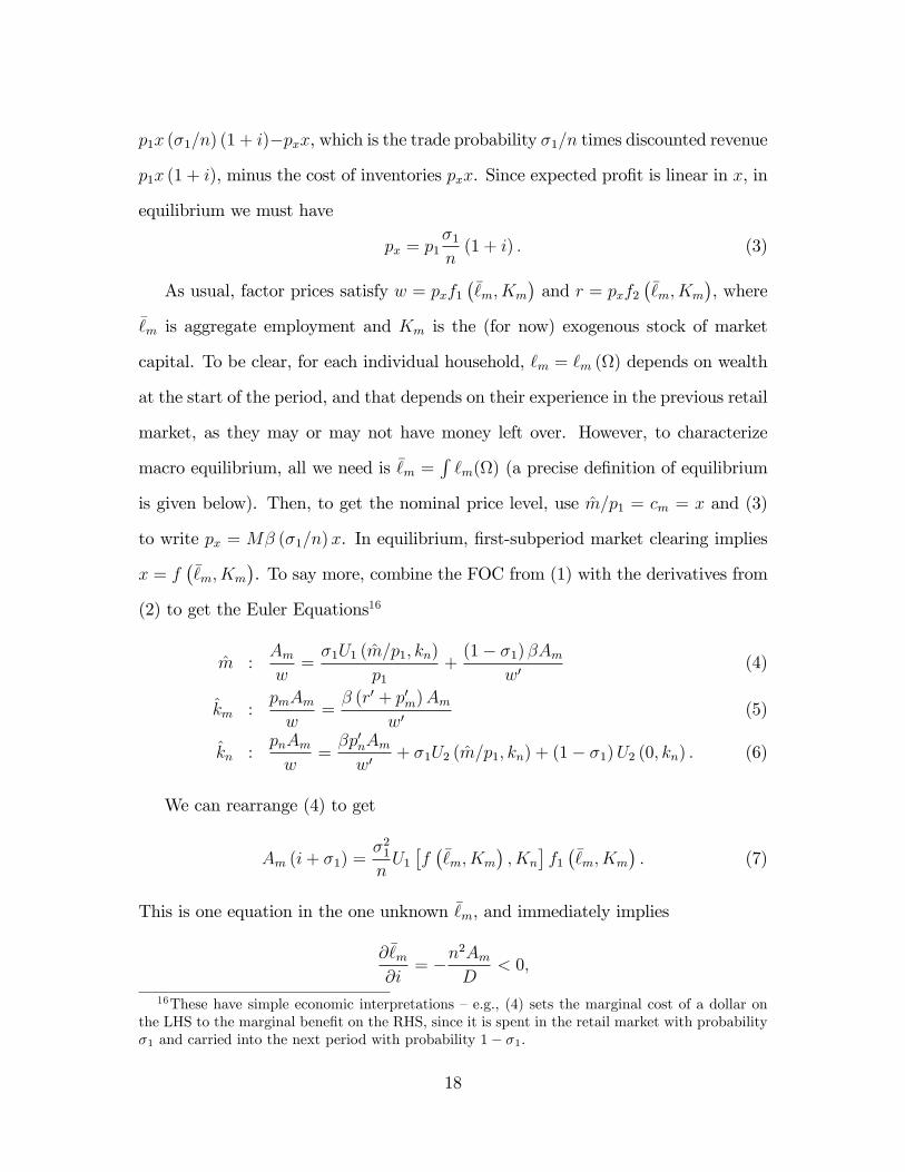
(2) to get the Euler Equations16

m :Amw=�1U1 (m=p1; kn)

p1+(1� �1) �Am

w0(4)

km :pmAmw

=� (r0 + p0m)Am

w0(5)

kn :pnAmw

=�p0nAmw0

+ �1U2 (m=p1; kn) + (1� �1)U2 (0; kn) : (6)

We can rearrange (4) to get

Am (i+ �1) =�21nU1�f��m; Km

�; Kn

�f1��m; Km

�: (7)

This is one equation in the one unknown �m, and immediately implies

@ �m@i

= �n2AmD

< 0;

16These have simple economic interpretations �e.g., (4) sets the marginal cost of a dollar onthe LHS to the marginal bene�t on the RHS, since it is spent in the retail market with probability�1 and carried into the next period with probability 1� �1.

18

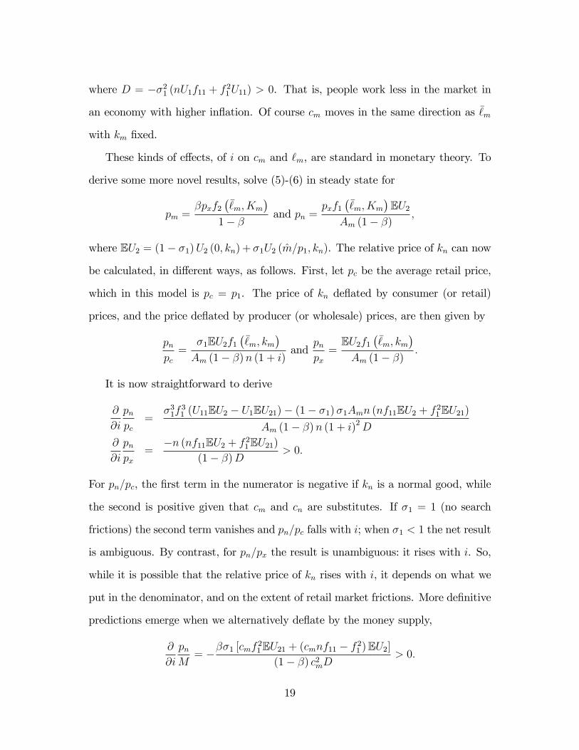
where D = ��21 (nU1f11 + f 21U11) > 0. That is, people work less in the market in

an economy with higher in�ation. Of course cm moves in the same direction as �m

with km �xed.

These kinds of e¤ects, of i on cm and `m, are standard in monetary theory. To

derive some more novel results, solve (5)-(6) in steady state for

pm =�pxf2

��m; Km

�1� � and pn =

pxf1��m; Km

�EU2

Am (1� �);

where EU2 = (1� �1)U2 (0; kn) + �1U2 (m=p1; kn). The relative price of kn can now

be calculated, in di¤erent ways, as follows. First, let pc be the average retail price,

which in this model is pc = p1. The price of kn de�ated by consumer (or retail)

prices, and the price de�ated by producer (or wholesale) prices, are then given by

pnpc=

�1EU2f1��m; km

�Am (1� �)n (1 + i)

andpnpx=EU2f1

��m; km

�Am (1� �)

:

It is now straightforward to derive

@

@i

pnpc

=�31f

31 (U11EU2 � U1EU21)� (1� �1)�1Amn (nf11EU2 + f 21EU21)

Am (1� �)n (1 + i)2D@

@i

pnpx

=�n (nf11EU2 + f 21EU21)

(1� �)D > 0:

For pn=pc, the �rst term in the numerator is negative if kn is a normal good, while

the second is positive given that cm and cn are substitutes. If �1 = 1 (no search

frictions) the second term vanishes and pn=pc falls with i; when �1 < 1 the net result

is ambiguous. By contrast, for pn=px the result is unambiguous: it rises with i. So,

while it is possible that the relative price of kn rises with i, it depends on what we

put in the denominator, and on the extent of retail market frictions. More de�nitive

predictions emerge when we alternatively de�ate by the money supply,

@

@i

pnM= ���1 [cmf

21EU21 + (cmnf11 � f 21 )EU2]

(1� �) c2mD> 0:

19

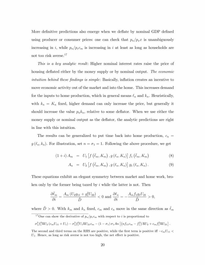
More de�nitive predictions also emerge when we de�ate by nominal GDP de�ned

using producer or consumer prices: one can check that pn=pxx is unambiguously

increasing in i, while pn=pccm is increasing in i at least as long as households are

not too risk averse.17

This is a key analytic result : Higher nominal interest rates raise the price of

housing de�ated either by the money supply or by nominal output. The economic

intuition behind these �ndings is simple: Basically, in�ation creates an incentive to

move economic activity out of the market and into the home. This increases demand

for the inputs to home production, which in general means `n and kn. Heuristically,

with kn = Kn �xed, higher demand can only increase the price, but generally it

should increase the value pnkn, relative to some de�ator. When we use either the

money supply or nominal output as the de�ator, the analytic predictions are right

in line with this intuition.

The results can be generalized to put time back into home production, cn =

g (`n; kn). For illustration, set n = �1 = 1. Following the above procedure, we get

(1 + i)Am = U1�f��m; Km

�; g (`n; Kn)

�f1��m; Km

�(8)

An = U2�f��m; Km

�; g (`n; Kn)

�g1 (`n; Kn) : (9)

These equations exhibit an elegant symmetry between market and home work, bro-

ken only by the former being taxed by i while the latter is not. Then

@ �m@i

=Am (U2g11 + g

21U22)

~D< 0 and

@`n@i

= �Amf1g1U21~D

> 0;

where ~D > 0. With km and kn �xed, cm and cn move in the same direction as �m17One can show the derivative of pn=pccm with respect to i is proportional to

�31f31EU2 (cmU11 + U1)� �31f31U1EU21cm � (1� �1)�1An

��nf11cm � f21

�EU2 + cmf21EU21

�:

The second and third terms on the RHS are positive, while the �rst term is positive i¤�cmU11 <U1. Hence, as long as risk averse is not too high, the net e¤ect is positive.

20

and `n. Hence, increases in i lower market work and consumption, and raise home

work and consumption. Increases in i also raise pn=px and pn=M .

4.2 Quantity E¤ects

The second simple model maintains n = �1 = 1 and cx = 0, but now market and

home capital are endogenous. As in standard growth theory, both market and home

capital are the same physical objects as output.18 We now present the equilibrium

equations, without derivation, since they are special cases of the general model

discussed below. First, we have two conditions for `m and `n, exactly like (8)-(9) in

the �rst simple model,

(1 + i)Am = U1(cm; cn)f1��m; km

�(10)

An = U2(cm; cn)g1 (`n; kn) : (11)

Next, we have steady state versions of the Euler Equations for km and kn,

�+ �m = f2��m; km

�(12)

�+ �n = f1��m; km

�U2(cm; cn)g2 (`n; kn) : (13)

Then we have the feasibility conditions,

cm = f��m; km

�� �mkm � �nkn (14)

cn = g (`nkn) : (15)

One can di¤erentiate (10)-(15) to get

D@kn@i

= � jf jU2g2�U2g11 + g

21U22

�� f1U2U21 (g1g21 � g2g11) [(f2 � �m) f21 � f1f22]

18This is the speci�cation in most home production models going back to Benhabin et al. (1991).What is missing here from the general model presented below is the following: a technology forproducing houses by combining structures and land, which allows us to go beyond pn=px = 1;search frictions; retail credit; and the consumption good cx.

21

where D > 0 and jf j � f11f22� f 212. The �rst term on the RHS is nonnegative, and

vanishes if f displays constant returns, while the second is positive given that cm and

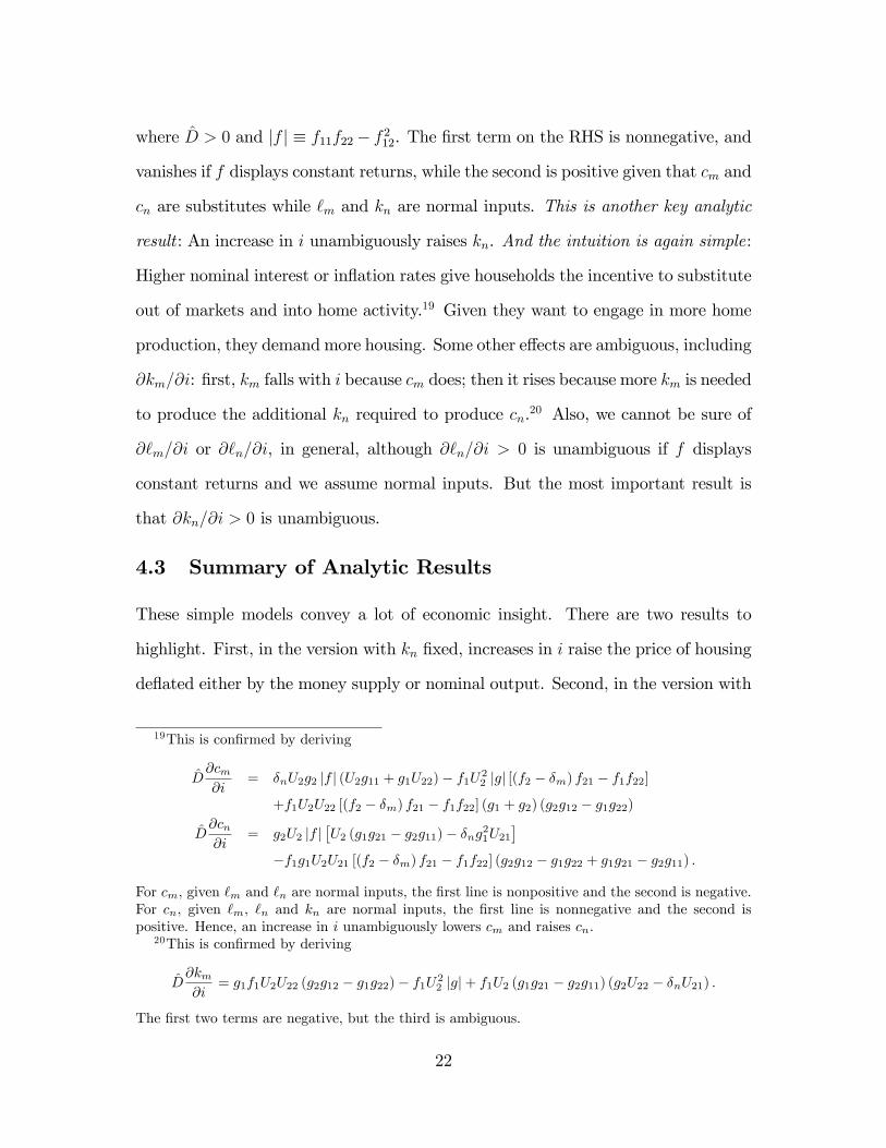
cn are substitutes while `m and kn are normal inputs. This is another key analytic

result : An increase in i unambiguously raises kn. And the intuition is again simple:

Higher nominal interest or in�ation rates give households the incentive to substitute

out of markets and into home activity.19 Given they want to engage in more home

production, they demand more housing. Some other e¤ects are ambiguous, including

@km=@i: �rst, km falls with i because cm does; then it rises because more km is needed

to produce the additional kn required to produce cn.20 Also, we cannot be sure of

@`m=@i or @`n=@i, in general, although @`n=@i > 0 is unambiguous if f displays

constant returns and we assume normal inputs. But the most important result is

that @kn=@i > 0 is unambiguous.

4.3 Summary of Analytic Results

These simple models convey a lot of economic insight. There are two results to

highlight. First, in the version with kn �xed, increases in i raise the price of housing

de�ated either by the money supply or nominal output. Second, in the version with

19This is con�rmed by deriving

D@cm@i

= �nU2g2 jf j (U2g11 + g1U22)� f1U22 jgj [(f2 � �m) f21 � f1f22]

+f1U2U22 [(f2 � �m) f21 � f1f22] (g1 + g2) (g2g12 � g1g22)

D@cn@i

= g2U2 jf j�U2 (g1g21 � g2g11)� �ng21U21

��f1g1U2U21 [(f2 � �m) f21 � f1f22] (g2g12 � g1g22 + g1g21 � g2g11) :

For cm, given `m and `n are normal inputs, the �rst line is nonpositive and the second is negative.For cn, given `m, `n and kn are normal inputs, the �rst line is nonnegative and the second ispositive. Hence, an increase in i unambiguously lowers cm and raises cn.

20This is con�rmed by deriving

D@km@i

= g1f1U2U22 (g2g12 � g1g22)� f1U22 jgj+ f1U2 (g1g21 � g2g11) (g2U22 � �nU21) :

The �rst two terms are negative, but the third is ambiguous.

22

kn produced like km in standard capital theory, increases in i raise the housing stock.

Intuitively, higher i is a higher tax on market activity; this makes households more

inclined to move into home production; this increases demand for inputs to home

production; and that leads to a rise in housing price or quantity.

The theory is also remarkably tractable, allowing us to either generate unam-

biguous predictions, or, when they are ambiguous, to see clearly the di¤erent e¤ects.

This is despite a rich structure, with home plus market production, multiple cap-

ital goods and frictional retail markets. For the rest of this paper, however, we

generalize the environment and study it numerically. The generalizations are im-

portant for matching some facts, including the relationship between real balances

and i, information on retail payment methods, and retail markups. Matching these

facts is important for the applications at hand, because they concern the impact of

monetary policy, and it improves con�dence in the theory when it performs well in

terms of standard monetary observations. Also, we bring back the technology for

production of housing kn = h (ks; kl), which is important because then increases in

demand can a¤ect both the price and quantity of housing.

Before moving to the general model, however, at the request of a referee, we

explain the method as follows. One endogenous variable on which we focus in the

calibration exercise is pnkn=pxx, where we show it increases in i (a similar discussion

applies to another variable on which we focus, pnkn=M). In theory one can decom-

pose a change in this variable into the changes in each component, pn, kn, px and x.

From the analysis presented above, heuristically, an increase in i raises pn=px and kn

and reduces x, all of which contribute to the increase in pnkn=pxx. While one might

want to consider each component in the data when evaluating the theory, it only

makes sense to consider stationary objects. One might hope that at least pn=px and

kn=x are stationary, but this is not true in our data. In principle, we could build a

23

model capturing the trends, but that goes beyond the current project. Hence, we

concentrate on pnkn=pxx, which is stationary in our data.21

5 The General Model

The state variable in the �rst subperiod now includes z = (m; b; km; ks; kl) plus

outstanding debt from the previous period d, since some retail purchases are now

made on credit (with quasi-linear utility we can restrict attention to one-period debt

without loss in generality). Also, given we bring cx back, it is purchased in the �rst

subperiod and becomes a state variable in the second. Hence, we writeW (z; d) and

V (z; cx) for the value functions. The generalization of (1) is then

W (z; d) = maxz;cx

�Am

w� Amw(m+ pxcx + pbb+ pxkm + pxks + plkl) + V (z; cx)

�;

where now = [r + px (1� �m)] km + px (1� �s) ks + plkl +m + b� T � d. Notice

x, km and ks have the same price px, since they are the same physical good, but the

price of housing pn is generally di¤erent. There are two equivalent ways to think

about housing in this context. For now we assume households build their own homes

using purchases of ks and kl, but the outcome is exactly the same if they instead

buy houses from construction �rms, as discussed below. The important results are

that again W is linear in and z is independent of .

To proceed, we need to discuss the second subperiod in more detail. There are

now three events that may occur for a household in the second subperiod: with

probability �0 they have no opportunity to trade; with probability �1 they have an

21Although we cannot decompose in the data the change in pnkn=pxx, we can in the model atsteady state. By way of preview, in Calibration 1 below, 84% of the change in pnkn=pxx comesfrom a decline in x, 4% comes from an increase in pn=px and 12% from an increase in kn; and inCalibration 2, 65% of the change comes from a decline in x, 9% comes from an increase in pn=pxand 26% from an increase in kn. So while we are getting a sizable e¤ect from a fall in x, bothpn=px and kn also behave in a way consistent with economic intuition.

24

opportunity to trade using money; and with probability �2 they have an opportunity

to trade using money or credit. Conditional on each event j, denote the value

function by V j(z; cx), and write V (z; cx) = �j�jV j(z; cx). As in the simple model,

when credit is not available, in money-only trade, households cash out. When credit

is available, both buyers and sellers are indi¤erent between cash and credit as long as

the value of the payment is the same, so without loss of generality assume they use

credit only. This is all standard. What is more complicated is that households choose

home work after knowing retail market outcomes, so there are di¤erent choices for

(cn; `n) in the cross section each period.22

For a household with no retail opportunity, c0m = 0 and

V 0 (z; cx) = maxc0n;`

0n

�u�cx; 0; c

0n

�� An`0n + �W (z)

st c0n = g(`

0n; kn)

where it is understood that kn = h(ks; kl). In this case, (c0n; `0n) satis�es the con-

straint and the FOC An = u3g1. For a household with a cash-only opportunity,

c1m = m=p1 and

V 1 (z; cx) = maxc1n;`

1n

�u�cx; m=p1; c

1n

�� An`1n + �

�W (z)� mAm

w0

��st c1n = g(`

1n; kn):

In this case the solution satis�es the constraint and the FOC An = u3g1. Finally,

for a household with a credit opportunity,

V 2 (z; cx) = maxc2n;`

2n

�u�cx; c

2m; c

2n

�� An`2n + �

�W (z)� p2c2m

Amw0

��st c2n = g(`

2n; kn)

where p2 is the retail credit price, which generally may di¤erent from the cash

price p1. In this case the solution satis�es u2 = p2�Am=w0 and An = u3g1. Again,

naturally, di¤erent outcomes in the retail market induce di¤erent outcomes for home

production.

22One can alternatively assume `n is decided before knowing the outcome in the retail market,but that seems less natural.

25

It is now routine to derive the household�s conditions generalizing (4)-(6),

m :Amw=�1u2 (cx; c

1m; c

1n)

p1+(1� �1) �Am

w0(16)

b :pbAmw

=�Amw0

(17)

km :pxAmw

=� [r0 + (1� �m) p0x]Am

w0(18)

ks :pxAmw

= h1(ks; kl)Eu2g2 +� (1� �s) p0xAm

w0(19)

kl :plAmw

= h2(ks; kl)E (u2g2) +�p0lAmw0

(20)

cx :pxAmw

= Eu1; (21)

where Eu1 = �j�ju1(cx; cjm; cjn) and Eu2g2 = �j�ju3(cx; cjm; cjn)g2(`jn; kn). Retailers

again purchase x and convert it one-for-one into second-subperiod goods, but now

they sell it for cash with probability �1=n and for credit with probability �2=n.

Given unsold inventories fully depreciate c1m = c2m = x, so the quantity is the same

in cash and credit transactions, but the price is not. Generalizing (3), we have

px =�1p1 + �2p2n (1 + i)

: (22)

Retailers are happy to bring any inventory x to the market when (22) holds.

As in the simple models, the price vector p = (w; r; px; pl; pb; p1; p2) can be

expressed in terms of the allocation. For factor prices, w = pxf1��m; km

�and

r = pxf1��m; km

�. For land, (20) implies it is priced by its capitalized value as an

input to housing, which is itself an input to home production,

pl =h2 (ks; kl)E (u2g2)w

(1� �)Am: (23)

Notice on the RHS dividing by Am and multiplying by w converts utils into time

and time into money. For cash retail purchases we have p1c1m = m = (1 + �)M , and

for credit retail purchases u2 (cx; c2m; c2n) = p2�Am=w

0. Hence, p1 = (1 + �)M=c1m

26

and p2 = (1 + i)u2 (cx; c2m; c2n)w=Am. Finally, (22) delivers the nominal price level.

This determines p as a function of the allocation. We now pare down the descrip-

tion of an allocation. In terms of land, structures and housing, since kl = Kl and

kn = h (ks; Kl), we need only keep track of kn. In terms of consumption, we have

c0m = 0, c1m = c

2m = x and c

jn = g[`

jn; h (ks; 1)]. Therefore, we can fully describe an

allocation by purchases of �rst-subperiod goods by households and retailers, market

and home capital, and market and home work, say a = (cx; x; km; kn; �m; `jn).

Formally, we have the following:

De�nition 1 A steady state equilibrium is an allocation and price vector (a;p)

satisfying: the FOC�s for home work

An = u3[cx; cjm; g(`

jn; kn)]g1(`

jn; kn); (24)

where it is understood that c0m = 0 and c1m = c2m = x; steady state versions of the

investment Euler Equations (18)-(19)

�+ �m = f2��m; km

�(25)

�+ �s = f1��m; km

�h1 (ks; 1) (1 + �)Eu2

g2Am

; (26)

the money Euler Equation (16), which we rewrite as

Am (�1 + i) = (1 + i)�1u2�cx; x; c

1n

� wp1; (27)

the FOC for cx and aggregate feasibility

Am = f1��m; km

�Eu1 (28)

f��m; km

�= cx + nx+ �kkm + �sk

0s; (29)

and prices, which are determined as discussed above.

27

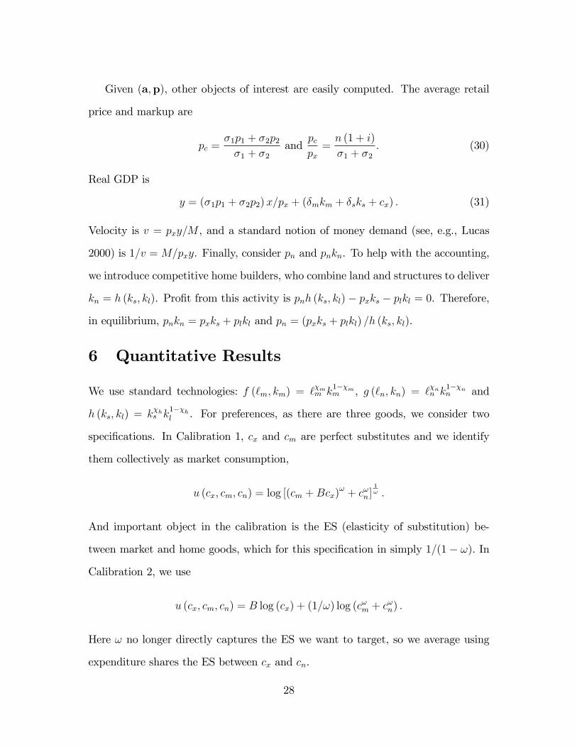
Given (a;p), other objects of interest are easily computed. The average retail

price and markup are

pc =�1p1 + �2p2�1 + �2

andpcpx=n (1 + i)

�1 + �2: (30)

Real GDP is

y = (�1p1 + �2p2)x=px + (�mkm + �sks + cx) : (31)

Velocity is v = pxy=M , and a standard notion of money demand (see, e.g., Lucas

2000) is 1=v =M=pxy. Finally, consider pn and pnkn. To help with the accounting,

we introduce competitive home builders, who combine land and structures to deliver

kn = h (ks; kl). Pro�t from this activity is pnh (ks; kl)� pxks � plkl = 0. Therefore,

in equilibrium, pnkn = pxks + plkl and pn = (pxks + plkl) =h (ks; kl).

6 Quantitative Results

We use standard technologies: f (`m; km) = `�mm k

1��mm , g (`n; kn) = `

�nn k

1��nn and

h (ks; kl) = k�hs k

1��hl . For preferences, as there are three goods, we consider two

speci�cations. In Calibration 1, cx and cm are perfect substitutes and we identify

them collectively as market consumption,

u (cx; cm; cn) = log [(cm +Bcx)! + c!n]

1! :

And important object in the calibration is the ES (elasticity of substitution) be-

tween market and home goods, which for this speci�cation in simply 1=(1� !). In

Calibration 2, we use

u (cx; cm; cn) = B log (cx) + (1=!) log (c!m + c

!n) :

Here ! no longer directly captures the ES we want to target, so we average using

expenditure shares the ES between cx and cn.

28

We use long-run observations to calibrate parameters when we can. Then, as

is standard in monetary models, we use properties of the empirical money demand

curve for some others, since for our experiments it is important that the model line

up well with standard monetary observations. Unless otherwise noted, our targets

are computed using U.S. data from 1975 to 1999, since we are not attempting to

explain the housing bubble. The length of a period is a quarter. The average

annual in�ation and T-bill rates are 4:13% and 6:80% in the sample, which yield

� = 0:0066 and � = 0:0103. We set �h = 0:73 to match the value of residential

structures plus durables relative to the value of housing capital. Then, to match the

investment �ows over the capital stocks for both km and ks we set �m = �s = 0:015,

which translates to 6% annual depreciation rates (it is a coincidence that they are

the same). We set �2 = 0:5�1 so that there are half as many retail trades made

on credit as there are in money, based on the data in the recent Bank of Canada

Methods of Payment Survey.23

A key element in any model with home production is the ES between market

and home goods. Benhabib et al. (1991) argue for an ES of 5, but in retrospect that

was probably too high. Estimates by Rupert et al. (1995) using PSID data yield

numbers closer to 1:8 or 2. Estimates by McGrattan et al. (1997) using aggregate

time series yield values between 1:5 and 1:8. Aguiar and Hurst (2007a) estimate

an ES of 1:8 from time-use data, while Chang and Schorfheide (2003) get a slightly

higher 2:3. While there is no single de�nitive number emerging from these papers,

there seems to be a consensus on a reasonable range. We pick an ES of 1:8. In

Calibration 1 this immediately implies ! = 0:44, while in Calibration 2 we need to

set ! together with the remaining parameters to match the targets jointly.

23As described in Arango and Welte (2012), the probabilities of using cash in any transactionfor single and married people are 55% and 48%, resp., and the probabilities of using credit cardsare 20% and 25%, resp., making �2 close to �1=2:

29

At this point, for Calibration 1 the parameters (Am; An; B; �m; �n; n; �1), and

for Calibration 2 these plus !, are calibrated to match the following targets. As is

standard (Greenwood et al. 1995) households spend on average �m = 33% of their

discretionary time working in the market and �n = 25% working in the home, while

market capital over annual output is km=y = 2:07 and household capital over annual

output is kn=y = 1:96. For the retail markup, we target 30% based on data from the

Annual Retail Trade Survey, following Faig and Jerez (2005). Finally, we match the

level and slope of money demand, targeting an average annual velocity of 5:76 and

a semi-elasticity with respect to i of 2:56%, obtained using a standard log-linear

regression. While the parameters are calibrated jointly, heuristically Am and An

match the hours targets, �m and �n match the capital-output ratios, n matches

the markup, B matches the level of velocity and �1 matches the money-demand

elasticity.24

The top panel of Table 2 reports the calibration results. In Calibration 2 ! is

0:83, which implies a large ES between cm and cn, but maintains the target ES

between overall market and nonmarket goods of 1:8. In terms of the retail market,

consider Calibration 1 (the other is similar). The measure of retailers is n = 0:22,

and the measure of households that trade each period is �1 + �2 = 0:17. Also,

(�1 + �2) =n, or 78%, is the fraction of retail inventories sold each period, while

the rest simply depreciate. About 15% of market consumption comes from retail,

cm; the rest, cx, is purchased directly from producers in the �rst subperiod. These

numbers are largely driven by the average velocity target, which cannot be matched

well without cx in the model. To understand the importance of home production, we

compute the percentage increase in market consumption required to compensate for

the loss if we force cn = `n = 0. For households that are able to trade in the retail

24Since the calibrations match the targets virtually exactly �i.e., up to many decimal points �we do not provide tables with targets and model-implied moments.

30

market, each period market consumption has to increase by 78% to compensate for

shutting down home production. For households that cannot trade in the retail

market, the number is 152%. Based on these observations, it is clear that it is

important to have all three goods, (cx; cm; cn), in the speci�cation.

6.1 Positive Results

We now ask how well the model accounts for the relationship discussed in Section 2

between nominal interest rates, on the one hand, and the value of home capital over

nominal output or over the money supply, on the other. Denote the value of home

capital over nominal output and over the money supply by H=Y and H=M . These

ratios are tightly connected to inverse velocity, Y=M , by the relationship H=M =

H=Y �Y=M . Since the average value of H=Y and Y=M are calibration targets, the

average value of H=M matches the data, by construction. The only elasticity we

target is the semi-elasticity of Y=M with respect to the nominal rate, denoted �Y=M .

The model generates endogenously a semi-elasticity forH=Y , denoted �H=Y , and the

elasticity of H=M then follows from �H=M = �H=Y + �Y=M . While we report both,

we think it more interesting to focus on �H=Y rather than �H=M , for the following

reason: Even if pnkn does not move at all, as long as real balances fall with i, we are

bound to get �H=M more or less right. It therefore seems more challenging �or, less

less mechanical �to focus on �H=Y .25

Table 2 reports the results and Figure 4 shows Y=M , H=Y and H=M versus i

for Calibrations 1 and 2 as well as the data. In Calibration 1 we get �H=Y = 0:25

and in Calibration 2 we get �H=Y = 0:57, or 22% and 52% of the semi-elasticities

in the data. When we consider �H=M , the model accounts between 78% and 87%

of the elasticity in the data, but again we prefer to focus on �H=Y . Whether we

25We compute a model-based semi-elasticity as the semi-elasticity at the calibrated steady stateusing numerical derivatives.

31

consider �H=Y or �H=M , it matters whether we use Calibration 1 or 2 �di¤erent

ways a disaggregating consumption are not equivalent, even if they hit the same ES

target. In any case, Figure 4 shows how the model tracks the broad patterns in the

data fairly well.

On the suggestion of the referees, we tried to establish some independent evi-

dence for a theory that says higher in�ation makes households substitute away from

market and into home production. First consider time allocation. Data imply semi-

elasticities of �0:6 and 0:2 for market and home labor, with respect to the nominal

interest rate.26 This is very much in line with the predictions of the theory, although

the corresponding numbers from the calibrated model are smaller, �0:2 and 0:04.

Still, this supports the general approach. In terms of consumption, there is no long

time series of home production, but we can present some corroborating evidence.

Take the ratio of �food and beverages purchased for o¤-premises consumption�and

�purchased meals and beverages,�where the former is an input to home production

and the latter is market consumption. Theory suggests this ratio should go up with

in�ation. The interest semi-elasticity of this ratio is 0:4.27 This also supports the

general approach.

Table 3 shows the �ndings are quite robust (in each case changing the calibration

as appropriate). Changing risk aversion from 1 to 1=2 or 2 has little e¤ect. The same

is true for increasing the calibration frequency to monthly or even weekly. This is

important because it is one of the reasons for modeling retail as a frictional market.

With a typical cash-in-advance model, e.g., households spend all their money each

period, so there is no way to match velocity when the period length is short. Here we

26For market labor we use hours-worked by prime-aged men between 1955-2005 from Francis andRamey (2009). For time spent in home production we use data from Ramey (2009) for employedmales between 1975-2003. Both of these series contain signi�cant trends that we removed linearly.

27This data covers the period 1955-2005, from Table 2.4.5 of the BEA, and in this case weremoved a cubic trend.

32

can shorten the period and keep everything basically the same by scaling the arrival

rates �j. In terms of the basic structure, one modi�cation we consider is setting

�h = 0 and thus removing home labor from the model. This only slightly weakens

the main result � �H=Y goes down from 0:25 to 0:19. As regards the ES target,

varying this in the range 1:5 to 2:3 yields roughly similar results. In Calibration 2,

if we use an ES of 5, we can account for 100% of �H=Y �but 5 is too high given the

empirical consensus. We prefer to conclude conservatively that the model accounts

for between 20% and 50% of the �H=Y relationship, which is clearly relevant, but

also leaves room for other factors.

6.2 Normative Results

We are also interested in the welfare e¤ects of in�ation. A standard exercise is to

compute the cost of in�ation as the amount of consumption households would be

willing to sacri�ce to go from 10% to the Friedman rule, which means an in�ation

rate consistent with a 0 nominal interest rate. A consensus estimate from reduced-

form analyses is that the answer is between 0:5% and 1:0%. By comparison, in

models along the lines of Lagos and Wright (2005), the number can be an order

of magnitude higher. One reason for the big e¤ects in those models is that they

use bargaining rather competitive pricing. Since it is well known that bargaining

matters, we instead consider the change in welfare e¤ects that come from adding

home production keeping pricing the same.28

Figure 5 shows how equilibrium changes with in�ation for the two benchmark

calibrations, as well as a version of the model with home production shut down. Since

in�ation is a tax on money holdings, higher in�ation reduces real balances, and hence

28See Aruoba et al. (2011) for a recent paper with references to work on the cost of in�ation.including price-taking and bargaining models. Note also that bargaining power is usually calibratedto match the markup in those models, but we get positive markups in the retail market even withcompetitive pricing due to the other frictions.

33

the demand by retailers for inventories, and hence employment and investment. In

the model without home production, market activity falls with in�ation, and this

creates a loss in welfare. In the model with home production, agents can make up

for some of the loss in cm by increasing cn. However, on net the cost of in�ation is

larger when home production is an option: going from 10% in�ation to the Friedman

rule implies a welfare gain of 0:4% without home production, 0:53% in Calibration

1, and 0:65% in Calibration 2. We conclude that incorporating home production

raises the cost of in�ation by somewhere between 1=3 and 2=3.

Again, an individual�s response to an increase in in�ation is to reduce market

and increase nonmarket activity. Depending on the how willing the individual is

to substitute between cm and cn, individual welfare may be minimally a¤ected by

this. However, relative to the no-home-production version, the ratio of cm to total

consumption spending is larger in the model with home production. This makes a

decrease in cm due to an increase in in�ation more costly and since they are only

imperfect substitutes, the increase in cn does not completely make up for the loss

in cm. In summary, for the cost of in�ation, home production makes a di¤erence.

While there is room for more work on the issue, it looks like the microfoundations

of household behavior matter, just like the microfoundations of monetary exchange

matter, for quantitative policy questions.

7 Conclusion

This paper reports our research on integrating models with money, home production,

and the production of homes. This is natural to the extent that monetary policy

provides incentives for agents to reallocate labor and capital between market and

household activity. In the data, we found that appropriately-scaled values of housing

wealth rise with in�ation or nominal interest rates. Theory generates analytic pre-

34

dictions that are qualitatively consistent with this. Our quantitative work showed

that calibrated models can account for some but not all of the observations. While

this leaves is room for other factors, the channel we highlight is clearly relevant. To

repeat what we said regarding the cost of in�ation, the results suggest strongly that

the microfoundations of household behavior matter, just like the microfoundations

of monetary economics matter, for monetary policy issues. That this not universally

understood or accepted is evidenced by the fact that many models used for policy

analysis these days pay little or no attention to these microfoundations. We hope

our results encourage at least some people to further pursue more detailed models

of monetary exchange and household behavior.

References

[1] Aguiar, M. and E. Hurst, 2005, �Consumption versus Expenditure,� Journalof Political Economy 113, 919-48.

[2] Aguiar, M. and E. Hurst, 2007a, �Life-Cycle Prices and Production,�AmericanEconomic Review 97, 1533-59.

[3] Aguiar, M. and E. Hurst, 2007b, �Measuring Trends in Leisure: The Allocationof Time over Five Decades,�Quarterly Journal of Economics 122, 969-1006.

[4] Arango, C. and A. Welte, 2012, �The Bank of Canada�s 2009 Methods of Pay-ment Survey: Methodology and Key Results,�Bank of Canada Working Paper.

[5] Albanesi, S. and C. Olivetti, 2009, �Home Production, Market Production andthe Gender Wage Gap: Incentives and Expectations,� Review of EconomicDynamics 12, 80-107.

[6] Albrecht, J., A. Anderson, E. Smith and S. Vroman, 2007, �OpportunisticMatching In The Housing Market,� International Economic Review 48, 641-64.

[7] Andre, C., 2010, �A Bird�s Eye View of OECD Housing Markets,� OECDEconomics Department Working Paper 746.

[8] Aruoba, S.B., C.J. Waller and R. Wright, 2011, �Money and Capital,�Journalof Monetary Economics 58, 98-116.

35

[9] Baxter, M. and U.J. Jermann, 1999, �Household Production and the ExcessSensitivity of Consumption to Current Income,�American Economic Review89, 902-20.

[10] Baxter, M., 2010, �Detecting Household Production,�manuscript, BU.

[11] Berentsen, A., G. Menzio and R. Wright, 2011, �In�ation and Unemploymentin the Long Run,�American Economic Review 101, 371-398

[12] Becker, G.S., 1965, �A Theory of the Allocation of Time,�Economic Journal75, 493-508.

[13] Becker, G.S., 1988, �Family Economics and Macro Behavior,�American Eco-nomic Review 78, 1-13.

[14] Benhabib, J., R. Rogerson and R. Wright, 1991, �Homework in Macroeco-nomics: Household Production and Aggregate Fluctuations,�Journal of Polit-ical Economy 99, 1166-1187.

[15] Brunnermeier, M.K. and C. Julliard, 2008, �Money Illusion and Housing Fren-zies,�Review of Financial Studies 21, 135-80.

[16] Burnside, M. Eichenbaum and S. Rebelo, 2011, �Understanding Booms andBusts in Housing Markets,�manuscript.

[17] Caplin, A. and J. Leahy, 2008, �Trading Frictions and House Price Dynamics,�manuscript, NYU.

[18] Chang, Y. and F. Schorfheide, 2003, �Labor-Supply Shifts and Economic Fluc-tuations,� Journal of Monetary Economics 50, 1751-1768.

[19] Chiu, J. and M. Molico, 2010, �Liquidity, Redistribution, and the Welfare Costof In�ation,�Journal of Monetary Economics 57, 428-438.

[20] Chiu, J. and M. Molico, 2011, �Uncertainty, In�ation, and Welfare,�Journalof Money, Credit and Banking 43, 487-512.

[21] Coulson, N.E. and L.M. Fisher, 2009, �Housing Tenure and Labor MarketImpacts: The Search Goes On,�Journal of Urban Economics 65, 252-64.

[22] Christiano, L.J., M. Eichenbaum and C.L. Evans, 2005, �Nominal Rigiditiesand the Dynamic E¤ects of a Shock to Monetary Policy,�Journal of PoliticalEconomy 113, 1-45.

[23] Cynamon, B.Z., D.H. Dutkowsky and B.E. Jones, 2006, �Rede�ning the Mon-etary Agggregates: A Clean Sweep,�Eastern Economic Journal 32, 661-72.

36

[24] Davis, M.A., J.D.M. Fisher and T.M. Whited, 2014, �Macroeconomic Implica-tions of Agglomeration,�Econometrica, forthcoming.

[25] Davis, M.A. and J. Heathcote, 2005, �Housing And The Business Cycle,� In-ternational Economic Review 46, 751-84.

[26] Davis, M.A. and J. Heathcote, 2007, �The Price and Quantity of Land in theUnited States,�Journal of Monetary Economics 54, 2595-620.

[27] Dressler, S.J., 2011, �Money Holdings, In�ation, and Welfare in a CompetitiveMarket,�International Economic Review 52, 407-423.

[28] Einarsson, T. and M.H. Marquis, 1997, �Home Production with EndogenousGrowth,�Journal of Monetary Economics 39, 551-69.

[29] Faig, M. and B. Jerez, 2005, �A Theory of Commerce,�Journal of EconomicTheory 122, 60-99.

[30] Ferguson, N., 2008, The Ascent of Money: A Financial History of the World.Penguin Press HC.

[31] Fisher, J., 1997, �Relative Prices, Complementarities and Comovement amongComponents of Aggregate Expenditures,�Journal of Monetary Economics 39,449-74.

[32] Fisher, J., 2007, �Why Does Household Investment Lead Business Investmentover the Business Cycle?�Journal of Political Economy 115, 141-68.

[33] Follain, J.R., 1982, �Does In�ation A¤ect Real Behavior: The Case of Housing,�Southern Economic Journal 48, 570-82.

[34] Geromichalos, A., J.M. Licari and J. Suarez-Lledo, 2007, �Asset Prices andMonetary Policy,�Review of Economic Dynamics 10, 761-79.

[35] Gomme, P., F. Kydland and P. Rupert, 2001, �Home Production Meets Timeto Build,�Journal of Political Economy 109, 1115-31.

[36] Gomme, P., P. Rupert, R. Rogerson and R. Wright, 2004, �The Business Cycleand the Life Cycle,�NBER Macroeconomics Annual 19.

[37] Greenwood, J. and Z. Hercowicz, 1991, �The Allocation of Capital and Timeover the Business Cycle,�Journal of Political Economy 99, 1188-214.

[38] Greenwood, J., R. Rogerson and R. Wright, 1995, �Household Production inReal Business Cycle Theory,� in Frontiers of Business Cycle Theory, ed. T.Cooley, Princeton.

37

[39] Greenwood, J., A. Seshadri and M. Yorukoglu, 2005, �Engines of Liberation,�Review of Economic Studies 72, 109-33.

[40] Gronau, R., 1997, �The Theory of Home Production: The Past Ten Years,�Journal of Labor Economics 15, 197-205.

[41] He, C., R. Wright and Y. Zu, 2011, �Housing and Liquidity,�manuscript.

[42] Head, A. and H. Lloyd-Ellis, 2012, �Housing Liquidity, Mobility and the LabourMarket,�Review of Economic Studies, forthcoming.

[43] Holmstrom, B. and J. Tirole, 2011,. Inside and Outside Liquidity. MIT Press.

[44] House, C., J. Laitner and D. Stolyarov, 2008, �Valuing Lost Home ProductionOf Dual Earner Couples,�International Economic Review 49, 701-36.

[45] Kearl, J.R., 1979, �In�ation, Mortgages, and Housing,� Journal of PoliticalEconomy 87, 1115-38.

[46] Kydland, F.E. and E.C. Prescott, 1982, �Time to Build and Aggregate Fluc-tuations,�Econometrica 50, 1345-1370.

[47] Lagos, R. and R. Wright, 2005 �A Uni�ed Framework for Monetary Theoryand Policy Analysis�Journal of Political Economy 113, 463-84.

[48] Lester, B., A. Postlewaite and R. Wright, 2012, �Liquidity, Information, AssetPrices and Monetary Policy,�Review of Economic Studies 79, 1209-1238.

[49] Lucas, R.E., 2000, �In�ation and Welfare,�Econometrica 68, 247-74.

[50] McGrattan, E.R., R. Rogerson and R. Wright, 1997, �An Equilibrium Model ofthe Business Cycle with Household Production and Fiscal Policy,�InternationalEconomic Review 38, 267-90.

[51] Mian, A., and A. Su�, 2011, �House Prices, Home Equity-Based Borrowing, andthe US Household Leverage Crisis,�American Economic Review 101, 2132�56.

[52] Ngai, L.R. and S. Tenreyro, 2009, �Hot and Cold Seasons in the Housing Mar-ket,�manuscript, LSE.

[53] Ngai, L.R. and C.A. Pissarides, 2008, �Trends in Hours and Economic Growth,�Review of Economic Dynamics 11, 239-56.

[54] Nosal, E., and G. Rocheteau, 2011, Money, Payments, and Liquidity, MITPress.

38

[55] Novy-Marx, R., 2009, �Hot and Cold Markets,� Real Estate Economics 37,1-22.

[56] Parente, S.,R. Rogerson and R. Wright, 2000, �Homework in DevelopmentEconomics: Household Production and the Wealth of Nations,� Journal ofPolitical Economy 108, 680-7.

[57] Piazzesi, M. and M. Schneider, 2009, �Momentum Traders in the Housing Mar-ket: Survey Evidence and a Search Model,�AER Papers & Proceedings 99,406-11.

[58] Piazzesi, M. and M. Schneider, 2010, �In�ation and the Price of Real Assets,�manuscript, Stanford.

[59] Poterba, J. M., 1991, �House Price Dynamics: The Role of Tax Policy andDemography,�Brookings Papers on Economic Activity 22, 143-203.

[60] Ramey, V.A., 2009, �Time Spent in Home Production in the Twentieth-CenturyUnited States: New Estimates from Old Data,�Journal of Economic History,69, 1-47.

[61] Ramey, V.A. and N. Francis, 2009, �A Century of Work and Leisure,�AmericanEconomic Journal: Macroeconomics, 1, 189-224.

[62] Ríos-Rull, J.-V., 1993, �Working in the Market, Working at Home, and theAcquisition of Skills: A General-Equilibrium Approach,�American EconomicReview 83, 893-907.

[63] Reinhart, C. and K. Rogo¤, 2009, This Time is Di¤erent: Eight Centuries ofFinancial Folly. Princeton University Press.

[64] Rocheteau, G. and R. Wright, 2005, �Money in Search Equilibrium, in Com-petitive Equilibrium, and in Competitive Search Equilibrium,�Econometrica73, 175-202.

[65] Rogerson, R., 2009, �Market Work, Home Work, and Taxes: A Cross-CountryAnalysis,�Review of International Economics 17, 588-601.

[66] Rogerson, R. and J. Wallenius, 2009, �Micro and Macro Elasticities in a LifeCycle Model with Taxes,�Journal of Economic Theory 144, 2277-92.

[67] Rupert, P., R. Rogerson and R. Wright, 1995, �Estimating Substitution Elas-ticities in Household Production Models,�Economic Theory 6, 179-93.

[68] Rupert, P., R. Rogerson and R. Wright, 2000, �Homework in Labor Economics:Household Production and Intertemporal Substitution,�Journal of MonetaryEconomics 46, 557-79.

39

[69] Sanches, D. and S. Williamson, 2010, �Money and Credit with Limited Com-mitment and Theft,�Journal of Economic Theory 145, 1525-1549.

[70] Shiller, R., 2005, Irrational Exuberance, Princeton University Press.

[71] Venkateswaran, V. and R. Wright, 2013, �Pledgability and Liquidity: A NewMonetarist Model of Financial and Macroeconomic Activity,�NBER MacroAnnual, in press.

[72] Wheaton, W.C., 1990, �Vacancy, Search, and Prices in a Housing MarketMatching Model,�Journal of Political Economy 98, 1270-92.

[73] Williamson, S. and R. Wright, 2010a, �New Monetarist Economics: Methods,�FRB St Louis Rev. 92, 2010.

[74] Williamson, S. and R. Wright, 2010b, �New Monetarist Economics: Models,�Handbook of Monetary Economics, eds. B. Friedman and M. Woodford, Else-vier.

[75] Wong, R., 2012, �A Tractable Monetary Model under General Preferences,�Bank of Canada mimeo.

40

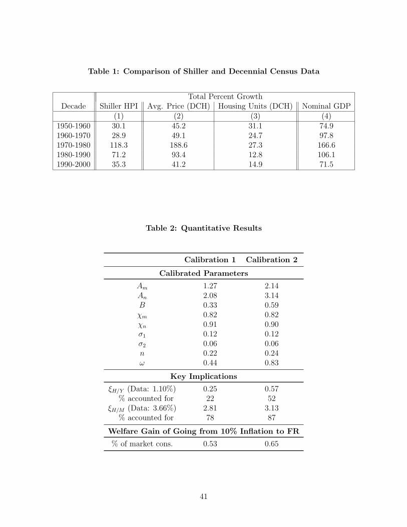
Table 1: Comparison of Shiller and Decennial Census Data

Total Percent GrowthDecade Shiller HPI Avg. Price (DCH) Housing Units (DCH) Nominal GDP

(1) (2) (3) (4)1950-1960 30.1 45.2 31.1 74.91960-1970 28.9 49.1 24.7 97.81970-1980 118.3 188.6 27.3 166.61980-1990 71.2 93.4 12.8 106.11990-2000 35.3 41.2 14.9 71.5

Table 2: Quantitative Results

Calibration 1 Calibration 2

Calibrated Parameters

Am 1.27 2.14An 2.08 3.14B 0.33 0.59χm 0.82 0.82χn 0.91 0.90σ1 0.12 0.12σ2 0.06 0.06n 0.22 0.24ω 0.44 0.83

Key Implications

ξH/Y (Data: 1.10%) 0.25 0.57% accounted for 22 52

ξH/M (Data: 3.66%) 2.81 3.13% accounted for 78 87

Welfare Gain of Going from 10% Inflation to FR

% of market cons. 0.53 0.65

41

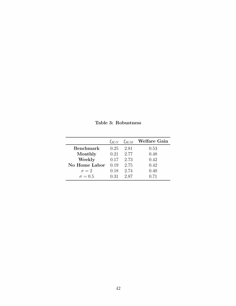
Table 3: Robustness

ξH/Y ξH/M Welfare Gain

Benchmark 0.25 2.81 0.53Monthly 0.21 2.77 0.48Weekly 0.17 2.73 0.42

No Home Labor 0.19 2.75 0.42σ = 2 0.18 2.74 0.40σ = 0.5 0.31 2.87 0.71

42

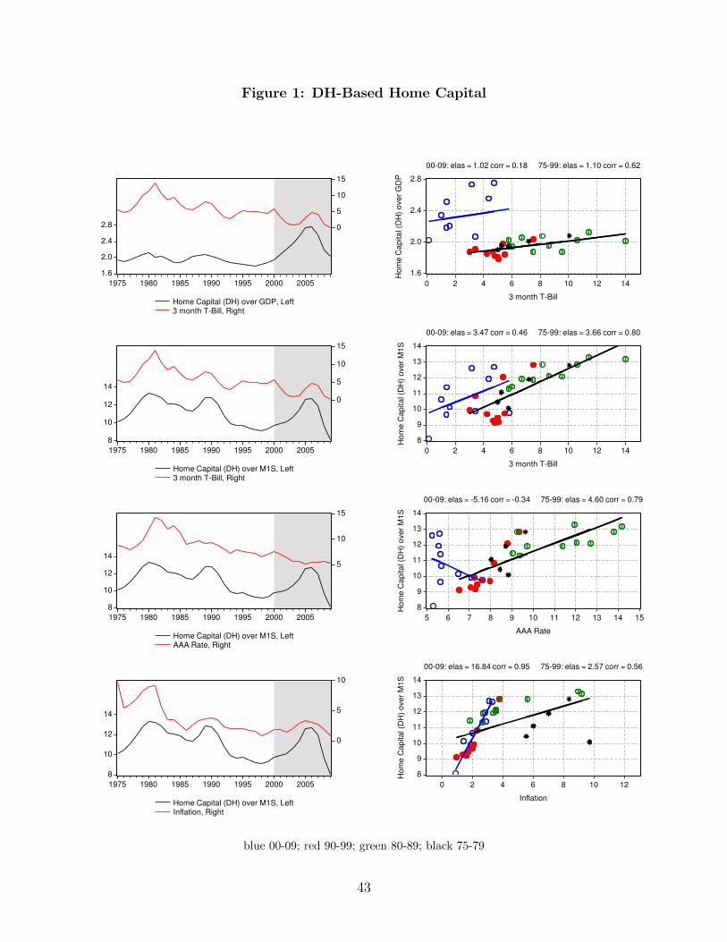
Figure 1: DH-Based Home Capital

1.6

2.0

2.4

2.8 0

5

10

15

1975 1980 1985 1990 1995 2000 2005

Home Capital (DH) over GDP, Left3 month T-Bill, Right

1.6

2.0

2.4

2.8

0 2 4 6 8 10 12 14

3 month T-Bill

Ho

me

Ca

pita

l (D

H)

ove

r G

DP

00-09: elas = 1.02 corr = 0.18 75-99: elas = 1.10 corr = 0.62

8

10

12

14

0

5

10

15

1975 1980 1985 1990 1995 2000 2005

Home Capital (DH) over M1S, Left3 month T-Bill, Right

8

9

10

11

12

13

14

0 2 4 6 8 10 12 14

3 month T-Bill

Ho

me

Ca

pita

l (D

H)

ove

r M

1S

00-09: elas = 3.47 corr = 0.46 75-99: elas = 3.66 corr = 0.80

8

10

12

145

10

15

1975 1980 1985 1990 1995 2000 2005

Home Capital (DH) over M1S, LeftAAA Rate, Right

8

9

10

11

12

13

14

5 6 7 8 9 10 11 12 13 14 15

AAA Rate

Ho

me

Ca

pita

l (D

H)

ove

r M

1S

00-09: elas = -5.16 corr = -0.34 75-99: elas = 4.60 corr = 0.79

8

10

12

14

0

5

10

1975 1980 1985 1990 1995 2000 2005

Home Capital (DH) over M1S, LeftInflation, Right

8

9

10

11

12

13

14

0 2 4 6 8 10 12

Inflation

Ho

me

Ca

pita

l (D

H)

ove

r M

1S

00-09: elas = 16.84 corr = 0.95 75-99: elas = 2.57 corr = 0.56

blue 00-09; red 90-99; green 80-89; black 75-79

43

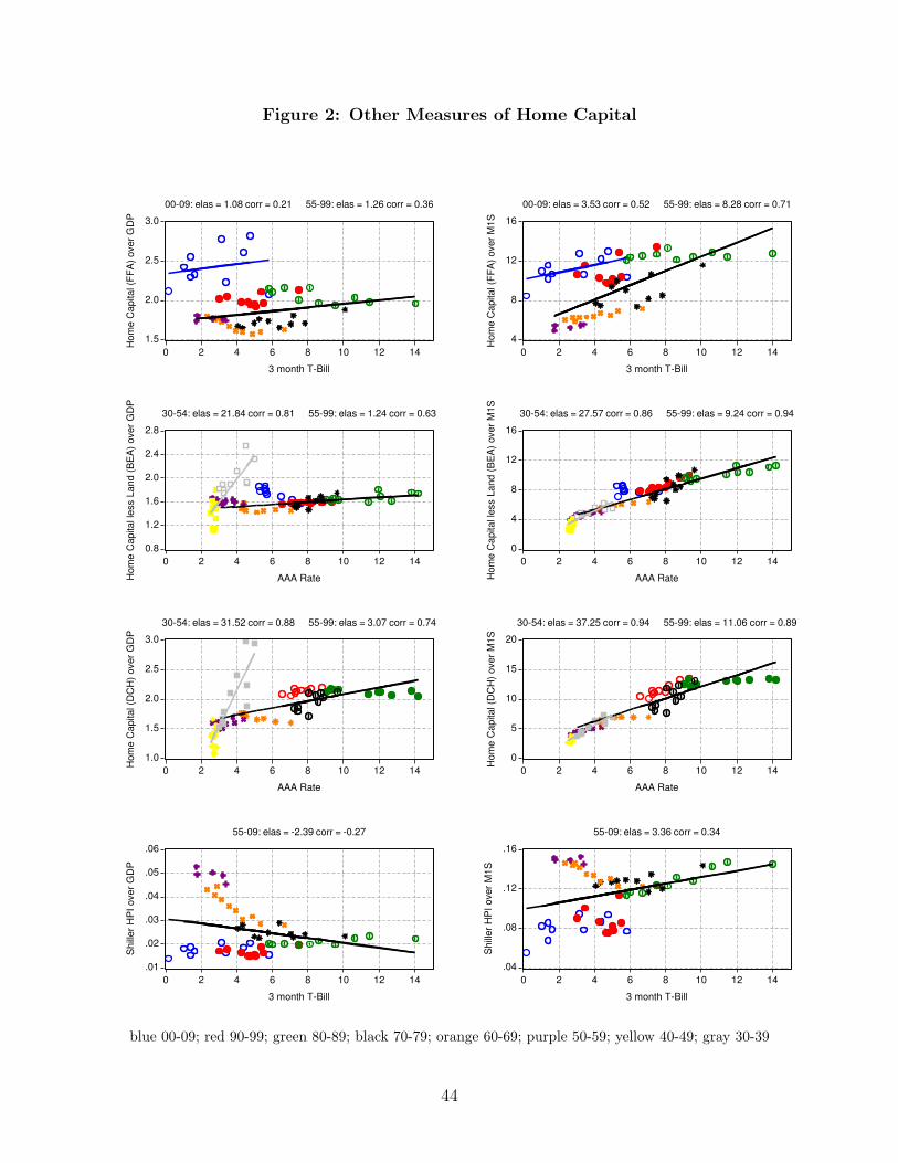
Figure 2: Other Measures of Home Capital

1.5

2.0

2.5

3.0

0 2 4 6 8 10 12 14

3 month T-Bill

Hom

e C

apital (F

FA

) over

GD

P

00-09: elas = 1.08 corr = 0.21 55-99: elas = 1.26 corr = 0.36

4

8

12

16

0 2 4 6 8 10 12 14

3 month T-Bill

Hom

e C

apital (F

FA

) over

M1S

00-09: elas = 3.53 corr = 0.52 55-99: elas = 8.28 corr = 0.71

0.8

1.2

1.6

2.0

2.4

2.8

0 2 4 6 8 10 12 14

AAA RateHom

e C

apital le

ss L

and (

BE

A)

over

GD

P

30-54: elas = 21.84 corr = 0.81 55-99: elas = 1.24 corr = 0.63

0

4

8

12

16

0 2 4 6 8 10 12 14

AAA RateHom

e C

apital le

ss L

and (

BE

A)

over

M1S

30-54: elas = 27.57 corr = 0.86 55-99: elas = 9.24 corr = 0.94

1.0

1.5

2.0

2.5

3.0

0 2 4 6 8 10 12 14

AAA Rate

Hom

e C

apital (D

CH

) over

GD

P

30-54: elas = 31.52 corr = 0.88 55-99: elas = 3.07 corr = 0.74

0

5

10

15

20

0 2 4 6 8 10 12 14

AAA Rate

Hom

e C

apital (D

CH

) over

M1S

30-54: elas = 37.25 corr = 0.94 55-99: elas = 11.06 corr = 0.89

.01

.02

.03

.04

.05

.06

0 2 4 6 8 10 12 14

3 month T-Bill

Shill

er

HP

I over

GD

P

55-09: elas = -2.39 corr = -0.27

.04

.08

.12

.16

0 2 4 6 8 10 12 14

3 month T-Bill

Shill

er

HP

I over

M1S

55-09: elas = 3.36 corr = 0.34

blue 00-09; red 90-99; green 80-89; black 70-79; orange 60-69; purple 50-59; yellow 40-49; gray 30-39

44

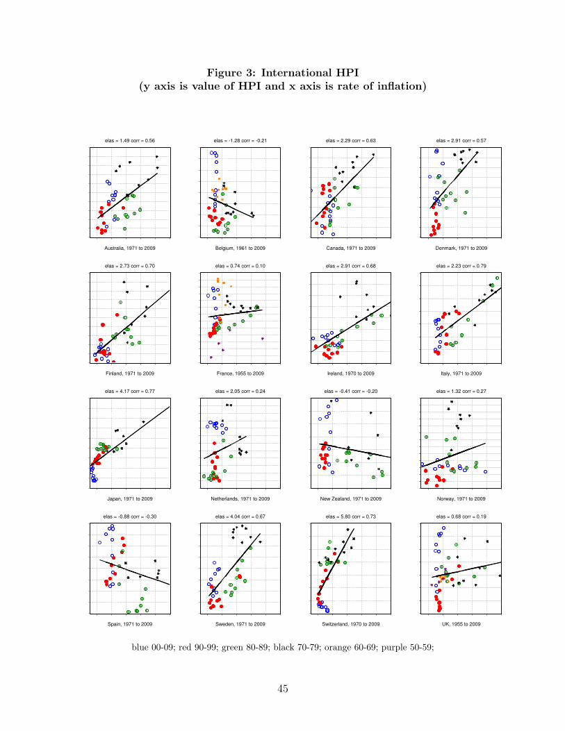
Figure 3: International HPI(y axis is value of HPI and x axis is rate of inflation)

elas = 1.49 corr = 0.56

Australia, 1971 to 2009

elas = -1.28 corr = -0.21

Belgium, 1961 to 2009

elas = 2.29 corr = 0.63

Canada, 1971 to 2009

elas = 2.91 corr = 0.57

Denmark, 1971 to 2009

elas = 2.73 corr = 0.70

Finland, 1971 to 2009

elas = 0.74 corr = 0.10

France, 1955 to 2009

elas = 2.91 corr = 0.68

Ireland, 1970 to 2009

elas = 2.23 corr = 0.79

Italy, 1971 to 2009

elas = 4.17 corr = 0.77

Japan, 1971 to 2009

elas = 2.05 corr = 0.24

Netherlands, 1971 to 2009

elas = -0.41 corr = -0.20

New Zealand, 1971 to 2009

elas = 1.32 corr = 0.27

Norway, 1971 to 2009

elas = -0.88 corr = -0.30

Spain, 1971 to 2009

elas = 4.04 corr = 0.67

Sweden, 1971 to 2009

elas = 5.80 corr = 0.73

Switzerland, 1970 to 2009

elas = 0.68 corr = 0.19

UK, 1955 to 2009

blue 00-09; red 90-99; green 80-89; black 70-79; orange 60-69; purple 50-59;

45

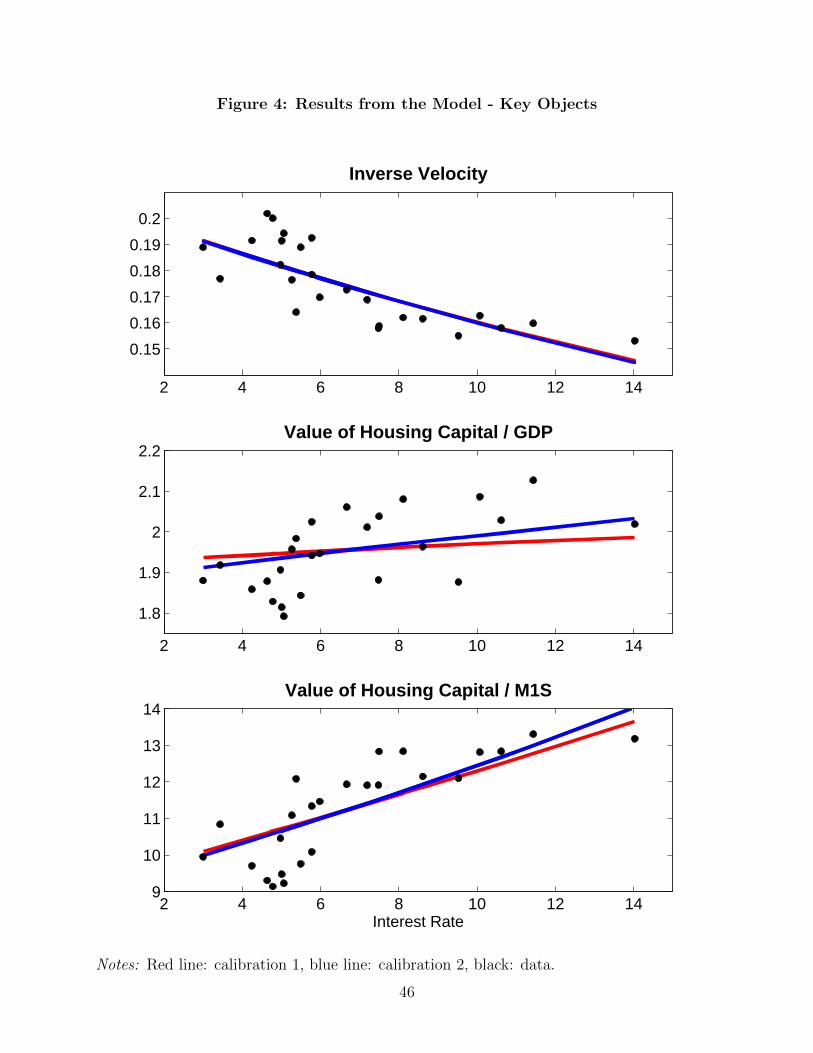
Figure 4: Results from the Model - Key Objects

2 4 6 8 10 12 14

0.15

0.16

0.17

0.18

0.19

0.2

Inverse Velocity

2 4 6 8 10 12 14

1.8

1.9

2

2.1

2.2Value of Housing Capital / GDP

2 4 6 8 10 12 149

10

11

12

13

14Value of Housing Capital / M1S

Interest Rate

Notes: Red line: calibration 1, blue line: calibration 2, black: data.

46

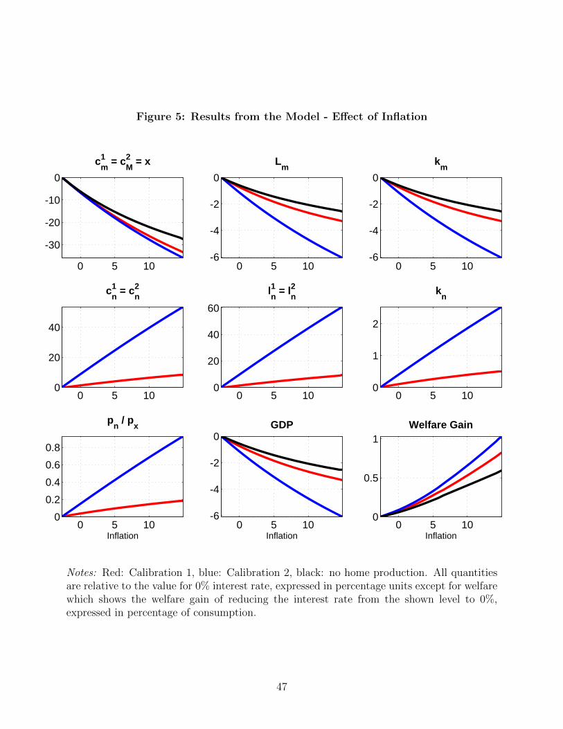
Figure 5: Results from the Model - Effect of Inflation

0 5 10

-30

-20

-10

0

c1m

= c2M

= x

0 5 10-6

-4

-2

0

Lm

0 5 10-6

-4

-2

0

km

0 5 100

20

40

c1n = c2

n

0 5 100

20

40

60

ln1 = l

n2

0 5 100

1

2

kn

0 5 100

0.2

0.4

0.6

0.8

pn / p

x

Inflation0 5 10

-6

-4

-2

0GDP

Inflation0 5 10

0

0.5

1Welfare Gain

Inflation

Notes: Red: Calibration 1, blue: Calibration 2, black: no home production. All quantitiesare relative to the value for 0% interest rate, expressed in percentage units except for welfarewhich shows the welfare gain of reducing the interest rate from the shown level to 0%,expressed in percentage of consumption.

47