Embed Size (px)
Citation preview

1
Homogeneous control and observation of uncertain SISO systems
Dalian, July 27, 2020 - Mexico, January 13, 2021 Avi Hanan, Adam Jbara, Arie Levant
Tel-Aviv University, Israel, http://www.tau.ac.il/~levant/

2
Numeric homogeneous differentiation of the 2nd order

3
Output stabilization problem of the relative degree n. ( , ( )) ( , ) ( , ) , ( , ) 0n
nddt
t x t h t x g t x u g t xs = + > The method
Uncertainty Þ differential inclusion (DI)
1 1( ) ( )nn
dnt nd
H G u- -sÎ s + sr r
Notation: ( ) )( , ,..., kks = s s s
r & Plan:
1. Control 1( )nu U -s=r
2. Differentiator 3. Method: homogeneity theory

4
Preliminary conclusions
· SISO homogeneous differential inclusions (disturbed integrator chains) of any homogeneous degree (HD) are robustly globally asymptotically stabilized by a standardized homogeneous output feedback.
· Non-Lyapunov control design is easy for any HD. · The feedback includes standardized filtering observers.
HGOs, SM-based differentiators are particular (non-filtering) cases for zero and negative HDs.
· The robustness is obtained with respect to bounded and some kinds of unbounded sampling noises.

5
References (July 2020): A. Bacciotti and L. Rosier. Liapunov Functions and Stability in Control Theory. Springer Verlag, London, 2005. E. Bernuau, D. Efimov, W. Perruquetti, and A. Polyakov. On an extension of homogeneity notion for differential inclusions. In Proc. of 12th European Control Conference ECC, 17-19 July, 2013, Zurich, pages 2204–2209, 2013. E. Cruz-Zavala and J.A. Moreno. Lyapunov approach to higher-order sliding mode design. In Recent Trends in Sliding Mode Control, pages 3–28. Institution of Engineering and Technology IET, 2016. E. Cruz-Zavala and J.A. Moreno. Lyapunov functions for continuous and discontinuous differentiators. IFAC-PapersOnLine, 49(18):660–665, 2016. E. Cruz-Zavala and J.A. Moreno. Levant’s arbitrary order exact differentiator: a Lyapunov approach. IEEE Transactions on Automatic Control, 64(7):3034–39, 2019. C. Qian. A homogeneous domination approach for global output feedback stabilization of a class of nonlinear systems. In Proceedings of the IEEE American Control Conference 2005, pages 4708–4715, 2005. W. Perruquetti, T. Floquet, and E. Moulay. Finite-time observers: application to secure communication., IEEE TAC, 53(1):356–360, 2008. L.K. Vasiljevic and H.K. Khalil. Error bounds in differentiation of noisy signals by high-gain observers. Systems & Control Letters, 57(10):856–862, 2008. ------------------ J.-P. Barbot, A. Levant, M. Livne, and D. Lunz. Discrete differentiators based on sliding modes. Automatica, 112: available online, 2020.
A. Hanan, A. Jbara, A. Levant. Homogeneous Output-Feedback Control, In Proc. of IFAC World Congress, July 13-17, Berlin, 2020. A. Levant. Higher order sliding modes, differentiation and output-feedback control. International J. Control, 76(9/10):924–941, 2003 A. Levant. Homogeneity approach to high-order sliding mode design. Automatica, 41(5):823–830, 2005
A. Levant. Non-Lyapunov homogeneous SISO control design. In 56th Annual IEEE Conference on Decision and Control (CDC) 2017, 6652–6657, 2017. A. Levant, D. Efimov, A. Polyakov, and W. Perruquetti. Stability and robustness of homogeneous differential inclusions. In Proc. of the 55th IEEE Conference on Decision and Control, Las-Vegas, December 12-14, 2016.
A. Levant and M. Livne. Robust exact filtering differentiators. European Journal of Control, available online, 2019. A. Levant, M. Livne, and X. Yu. Sliding-mode-based differentiation and its application. IFAC-PapersOnLine, 50(1):1699–1704, 2017. A. Levant and X. Yu. Sliding-mode-based differentiation and filtering. IEEE Transactions on Automatic Control, 63(9):3061–3067, 2018.

6
Homogeneity Basics

7
Weighted Homogeneity Homogeneity of a function f: Rn ® R
Dilation: x Î Rn, deg xi = mi > 0
dk: ),...,,(),...,,( 212121
nmmm
n xxxxxx nkkka deg f = q Û "x "k > 0 f(dkx) = kq f(x)
A function f is called a homogeneous norm if it is positive definite and deg f = 1.
Example: 1
11| | ... | |
dd dmm n
nhdx x xé ù
= + +ê úë û
, d > 0.

8
The homogeneity degree is defined up to proportionality
s > 0, k := k1s
kq = k1qs, kmi = k1
smi,
New weights are qs, mis

9
Homogeneity of differential inclusions Levant 2005
The homogeneity degree q = - p ( deg t = p ) iff "x "k > 0 (t, x) a( kpt, dkx)
preserves the differential inclusion (equation).
1
( ) ( ) ( )( )
( ) ( )
nxp
p
d d x F d x x F x Td t
F x d F d x
kk
-k k
Î Û Î Ìk
Þ = k
¡&
( )i ix f x=& Þ deg deg deg deg ( )i i i ix x t f x m p= - = = -&

10
Homogeneous arithmetic
1. deg( ) deg degA B A B+ = = 2. deg( ) deg degAB A B= + 3. deg( / ) deg degA B A B= -
4. deg( ) degA Ab = b 5. deg deg deg
i ix A A x¶¶ = -
6. deg deg( ) deg degxA A x A t¶¶= = -& &

11
Special power functions
signs s s sg ggë ù = @ 0 signs s=

12
Asymptotic Stability (AS) implies 1. Finite-Time (FT) Stability for 0q <
Example: § ¨2 2
3 31 13 3tan( sign ) | | [2,3] , 1, n qsÎ s s - s = = -&
2. Exponential stability for 0q = Example: [ 1,1] | | [2,3] , 1, 0n qsÎ - s - s = =& 3. Fixed Time (FxT) convergence from infinity to any
ball for 0q >
Example: § ¨4 43 3 1
3cos(sign ) | | [2,3] , 1, n qsÎ s s - s = =&

13
Back to stabilization

14
The homogeneity dominance/extension Uncertainty Þ homogeneous differential inclusion (DI)
1 1 1( ) ( ) ( )nn
dndt n nH G u- - -sÎ s + s sr r r
Homogeneity weights: ( )deg 1 , 0,..., , 1 0, degi iq i n nq t qs = + = + ³ = -
Rule: deg deg deg deg degddt f f f t f q= = - = +&
Homogeneous norm:
1 111 ( ) )|| max(| |,| | .| .,| . | |,q kq
k hk+ +
¥s = s s sr &

15
Homogeneous stabilization problem System output satisfies the DI
( ) 11[ , ] || || [ , ] ,
0, 0 ,
n nqn h m M
m M
C C K K uC K K
+-s Î - s +
³ < £
r
Only s is available, possibly with noise Solution:
stabilizer+ filtering observer/differentiator If 1 /q n= - obtain n-SMC problem
( ) [ , ] [ , ] ,nm MC C K K us Î - +
then filtering hybrid differentiator is used

16

17
Homogeneous Control Templates Theorem (Levant 2017):
AS DE: ( 1)1 2 1( ) 0, r
r r r C-- - -s + j s = j Î
r Sign equivalency: QC = quasi continuous, continuous everywhere accept 0 ( ): , QC , deg degr r
r r rf ® f Î f = s¡ ¡ ( 1)
1 1 1 20 sign ( ) sign[ ( )]rr r r r r
-- - - -s ¹ Þ f s = s + j s
r r r ( 1)
1 1 2| ( ) | | ( ) | 0rr r r r
-- - -f s + s + j s ¹
r r
Then for large enough , 0a b > get AS DE and DI ( )
1( ) 0rr r-s + bf s =
r
( )
1deg( )
1[ , ] ( )[ , ] || ||rr
r m M rh rC C K K -s
-s s - af sÎ -r r

18
Example: r-SMC design
( ) [ , ] [ , ] ,rm MC C K K us Î - +
General option: deg 1, deg t qs = = -
( ) 11deg 1 , 0,..., , 1 0, degi
riq i r rq t q +s = + = + = = - = Traditional weights:
( 1)deg , deg 1, ..., deg 1rr r -s = s = - s =&
Sign equivalency: § ¨ § ¨0 : A B A Bg g"g > + +∼

19
Example: 3-SMC design [ , ] [ , ] ,m MC C K K usÎ - +&&&
deg 3, deg 2, deg 1s = s = s =& &&
r = 1: § ¨2/30 0s + b s =& any 0 0b > fits
r = 2: § ¨2/30
2/30
1/2 1/31 | | | |tan max[| | ,| | ] 0s+b s
s +b ss + b s s =&
&&& &
§ ¨ § ¨1
2/31 202
2/30
11 162 4
1/2 1/31 | | | |
3
tan max[| | ,| | ]
| | | | | |SMu
s+b s
s +b s
-
s + b s s= -a
s + s + s
&&
© ¬% ª && &ª « ®&& &
tan s can be replaced with arctan 0.5sins s+

20
General form for r = 3: 13deg 1, deg 1 , deg 1 2 , q q qs = s = + s = + ³ -& &&
§ ¨ § ¨1
1 2 211102
10
1 2 1 212(1 )2 2
1 21 | | | |
3,
tan max[| | ,| | ]
| | | | | |
qqq
q
q qq
q
qu
+++
+
+ ++
s+b s +s +b s
s + b s s= -a
s + s + s
&&
© ¬% ª && &ª « ®
&& &
Any 0 0b > , then 1 , b a% are to be found by simulation
one by one for each q Note: 3 3, 1/3SMu u- -= !

21
(r+1)-SMC Design (Levant, Dorel –CDC2008)
( )
( 1)
( , ) ( , )( , ,..., )
r
rr
h t x g t x u
u U -
s = +
= a s s s&
Discontinuous control causes chattering
Nowadays (Moreno, Fridman, et al ): Continuous SMC
[ , ], | |d hm M dt gg K KÎ £ D

22
Simple HOSM chattering attenuation
( , ) ( , )x a t x b t x u= +& , u& = aUr+1(s, s& , ..., s(r)) s(r+1) = h1(t,x,u) + g(t,x) u&,
h1 = th¢+ xh¢ a + ( xh¢ b + tg ¢+ xg ¢ a)u + xg ¢ bu2. Required assumptions:
| th¢+ xh¢ a | £ ca, | xh¢ b + tg ¢+ xg ¢ a | £ cb, | xg ¢ b | £ cd
u& prevails for sure only for s » s& » ... » s(r) » 0 since u » ueq = - h(t,x)/g(t,x) is kept
Þ local convergence only

23
Alternative way (2008): Integral (r+1)-SMC Levant, Dorel CDC2008, IEEETAC 2007 (see the Levant’s homepage)
Choosing s(t) with desired trajectory: s(t, x(t)) = s(t), Initial conditions at t = t0: s(t0)=s(t0), s&(t0)=s& (t0), ..., s(r)(t0)=s(r)(t0)
s(t) = 0 with t ³ tf. | s(r+1)(t)| £ const SOLUTION: S(t, x) = s(t, x) - s(t) º 0 , The sliding mode starts from the very beginning.
Differentiator is directly applicable

24
Options for the trajectory choice:
1. Optimal trajectory (i.e. minimal transient time under a restriction on | s(r+1)(t)|)
2. Choice of the transient time as a function of initial conditions, and another optimization (optionally).
Levant, Alelishvilli, IEEETAC, 2007

25
New (2008) simple solution idea Auxiliary dynamic system:
s(r+1) = v, |v| £ a0 S = s - s,
s(t0) = s(t0), …, s(r)(t0) = s(r)(t0) u& = - aUr+1(S, S& , ..., S(r)),
a is sufficiently large Þ s º s, …, s(r) º s(r) v directly controls s, s& , ..., s(r)
v is the actual new bounded control

26
Integral HOSM chattering attenuation Thus the auxiliary control v directly dictates the chosen transient trajectory to s º 0. The original system does not affect it.
Theorem. Semi-global finite-time convergence to the (r+1)-sliding mode s º 0. Output-feedback control is readily produced.

27
Simulation (CDC 2008) x&& = - sin x + R(t) u, R(t) Î [0.5, 1.5], R = 2 + sin 4t, xc = 0.5 sin 0.5t + 0.5 cos t s = x-xc , r = 2 x(0) = -6, x&(0) = -15, u(0) = 3. u& = - 40 [S2+2(|S1|+|S0|2/3)-1/2(S1+|S0|2/3sign S0)]/[|S2|+2(|S1|+|S0|2/3)1/2];
s = x-xc, S0 = z0 – s, S1 = z1 - s&, S2 = z2 - s&& ; s&&& =-l320[s&& +2l3/2(|s&|+l|s|2/3)-1/2(s&+l|s|2/3sign s)]/ [|s&& |+2l3/2(|s&|+l|s|2/3)1/2], s(t0) = z0(t0), s&(t0) = z1(t0), s&& (t0) = z2(t0);
0z& = v0, v0 = - 18.5664 | z0 - s| 2/3 sign(z0 - s) + z1,
1z& = v1, v1 = - 42.4264 | z1 - v0| 1/2 sign(z1 - v0) + z2,
2z& = - 880 sign(z2 - v1). L = 800, z0(0) = s(0), z1(0) = z2(0) = 0

28
l = 0.8, e = 0 l = 0.5, e = 0
Control starts from t0 = 0.5 (for the differentiator convergence).
e is the noise magnitude. |s| £ 1.4×10⁻¹⁰, |s& | £ 6.0×10⁻⁷, |s&& | £ 0.007 are obtained with t = 10-5

29
The resulting Lipschitzian control for l = 0.5

30
l = 0.5, Noise: e = 0.01 l = 0.5, Noise: e = 0.001 s and s& (coordinates of the original system) demonstrate infinitesimal
chattering.

31
Observation Differentiation

32
“Standard” ndth-order differentiator (non-recursive form)
Levant 2003, Lyapunov function: Cruz-Zavala, Moreno 2017
§ ¨
§ ¨
§ ¨
11 1
11
1
21
11
0 0 1
1 1 0 2
( 1)0
1 1 0
0
( ) ,
( ) ,
... | | L
( ,
)
ndnd ndd
ndnd n
d
d
dd
nnd nd
d d
d
n
n
n n
n
n
z L z f t z
z L z f t z
f
z L z f t z
z
+
+ +
+-
+
+
-
+
-
= -l - +
= -l - +
£
= -l - +
= -l
%&
%&
%&
%& ( )0 0 ( ( )), 0.sign i
iL z f t z f- - ®

33
ndth-order homogeneous differentiator of the filtering order nf, 1 1
1d fn nq+- £ <
§ ¨
§ ¨
§ ¨
)| 11
| |
1
1)| |
1
(| 11
11
(11
(1
)| |
1
1 1 1 1 0
0 1 1
1
1 2
1
,
...
, ( ),
,
.
..
n qfn qf n qf
qfn qf n qf
qf qn qf n qf
qfn
q
d f
n
f d f f
n
d
n nd
d
n n
n n
d
n n
n
f
n
w
n
w L w
w L w w w z f t
z L w z
z Ln
--
-
+-
+
--
-
+
-
-
+
+ + +
-
= -l +
= -l + = -
= -l
éêêêêêê
l
ë
+
= -
%&
%&
%&
%& § ¨
§ ¨(
1
1)| |
1
1
(1 1)
10
1
1
,
.
qqf n qf
qf qn qf n q
dn
dn nd nd
df
n
n
w z
z L w
-
+
+
++ +
--
éêêêêêêêêê
+
ë = -l%&

34
Differentiator input: 0( ) ( ) ( )f t f t t= + h Differentiator: ( )
0 0( ) ( ( ),..., ( )), d
in if z z z f× × × »a
Exact convergence condition for h = 0:
( 1 )| | 1 ( 1)1 1
( )0
( 1)0 0,...,
1
]| ( ) |
, 0,1,...,
|
, ,
max |
0
( )[n i q n qd d
iq iqdd
ii i L
nL i
d
n i
nz f
f t t
i L
L+ - + ++ ++
=
z = - g
z
>
£ g
= ³
--------------------------------------------------------- 1 / ( 1)dq n= - + Þ ( 1)
0| ( ) |dnLf t L+ £ g , 0L >
------------------------------------------- 0Lg = Þ 0f is a polynomial, 0 0 1 ... d
d
nnf c c t c t= + + + .
------------------------------------------- 0q = Þ ( 1)
0 0| ( ) | || ( ,..., ) ||dd
nL nf t+ £ g z z

35
Recursive form, 1/nf ≥ q ≥ -1/(nd + 1) § ¨
§ ¨
1)1
2)1 (
1
1) 1 ( 1)
|
| | 1 (
| | 1
|1
(
11
1 2
2 2 1 3
1
1
1 1 1 01
0
,
...
, ( )
,
,
f
n qfn qf n qf
n qf
q
d f
q
d f
f d f f
n qf n qf
d
qf
n n
n n
n n n n n n
f
d
n
w L w
w L w w
w L w w w w z f t
z L
w
wn
n
-
-
-- -
- -
-
--
-
-
+
+ -
+-+ +
= -l +
= -l
éêêêê -êêêê - =êë
+
= -l + -
= -l
© ¬ª
&
& &
& ®&
&
«| |
1
| |1) ( 1)
| |
11
11 ( 1
1 ( 1)1 1
1 1
1 1
0
1 2
1
,
.
.
,
.
.f f
nd
d d d d
nd
d d d
q qn q n qd d
q qn q n qd d
n n
n n n n
n n n
w w z
z L z z z
z L z z
-
+
++ +
++ +
-
+
+
- - -
-
é-ê
êêêê -êêê
+
= -l +
= -ë -l
© ¬ª « ®
© ¬ª «
&
®
© ¬®& ª«
&
& &

36
Recursive coefficients
1 ( )1 ( 1)
1 ( 1)1 ( )
1
1
, where ;
, 1,2,..., ,
, , 1,..., .
n i qfn i qf
n i qdn i qd
d
k k d f
k i k i k i f
k i k i d dn i
k n n
i n
i n n k
- -
- - +
+ - ++ -
- - - +
- - - +
l = l = +
l = l × l =
l = l × l = +
%
% %
% %
Theorem. 0 1{ , ,..., }d fn n+$l = l l l
r for each gL > 0, L ≥ 1.
To find lr
perform proportional change of the homogeneity degrees: deg 1,0, deg deg deg 0
d dn nt z z t d= ± = - = ³&

37
Recursive form, deg t = 1, -1, d 0; deg t = 0, d § ¨
1 ( )1) 1)
1)12)(
(( )
( (
2
1
1
1 2
1
1
0
1
0
0
,
...
,
( ), 0 f
o ,r
d ndd
s
nd d ndd f
d ndd n d nd d
f d
n sf qn sf q n sf q
sqsq q
f f
f
f
f
n n
n n n
n
f
n n
d
n f
w L
n
w
w L w w w
w z n
w
n
f t w
z
- +-
++
- +
-
+
+- + - +
+
+ - +
+
= -l +
= -l +
= - =
= -l
éêêêêê -êê =êë
&
& &© ¬ª« ®
&
&
§ ¨
1
( 1 (
( 1)
1) 1)
1
1
1 1
1
0
1
2
0
,
,
, si
.
g
..
n
sqs sq q
f f
sqsq sq
d ndd n d nd d
d
d
d
ndd nd d nd
d
dd d
ds sq
dq
n
n
n n
n q
n
n
L w w z
z L z z z
z z s qL z
-- + - +
- --
-
- --
+ +
= -l +
ê
éê -êêê -êêêê - =ë = -l
&
& &
& &
© ¬ª « ®
© ¬ª « ®

38
Universal recursive coefficients 1/ | | ( 1)sign , 0,
1,, 0,
dq n q qd L
q+ + ¹ì
= ³í¥ =î
Theorem. 1q" ³ - , 0 Ll > g , 0d ³ , signqs q=
0, ( 1)d f qk n n d k s" = + ³ > + 0 1{ , ,..., ,...}k$l = l l lr
· 0q £ then lr
is infinite · 0q > then l
r is finite
0d = , then 1/ ( 1)dq n= - + and for 1Lg = {1.1,1.5,2,3,5,7,9,12,14,17,20,26,32,...}l =
r, 12k £

39
SMC case, q = -1/(nd + 1) The parameters 0 ,...,
d fn n+l l% % for 0,...,12d fn n+ = can be taken from the table

40
Filtering High-Gain Observer, q = 0 1
1 1
1 1 1 1 0
2
0 1 1
1 1 1
0 1
1 2
3
,
,
..., ( ),
,
...,
.
d f
d f
f d f f
d
d d
d
f
d
n n
n n
n n n n
n
n n
n
w
wn
w w
w w
w w w w z f t
z w z
z z
z w
nw
+
+ -
+ + +
-
éêêêêêêëéêêêêê
= -l +
= -l +
= -l + = -
= -l +
ë
= -l +
= -l
%&
%&
%&
%&
%&%&
( 1 )0ˆ d fn n k
k k- + + -l = l e% % , ˆ0 1< e << , k = 0,1,…,nd + nf
Hurwitz: 10 ,0 0,0( ) ...d f d f
d f
n n n nn np s s s+ + +
+= + l + + l% %

41
Bihomogeneous differentiator, 0 > q ≥ -1/(nd + 1) § ¨
§ ¨
( 1)1
2)1 (
| | 11
| |1) 1 ( 1)
|1
1
11
|
(
1 2
2 2 1 2 1 3
1 1
1 1
1 11 1
,
( )
..
,
.
( )
q
d f d f
q
d f d f
n
f d f f d
qfn qf n qf
n qfn q n
f f
f qf
qqq
n n n n
n n n n
n n n n n n n
f
w
wn
w L w Mw
w L w w M w w
w L w w M w w
-
-
-- -
-
-
--
-
-
-
+ +
+ - + -
+ +- -
= -l +
= -l +
= -l - m +
- m
- - m -
- -
&
& & &
& & ® &© ¬ª «1
1
11
|
(
|1
| |1) 1(
|
1
|1
)
1 1 0
0 1 1 1
1 1 1 2 1 1
0
2
(
, ( ),
) ,
...
( )
,
q qn q n qd d
qn
f f
d f f d f f
nd
d d d d d d
d
n n
n n n n n n
n n n n n nd
n
n
w w z f t
z L w w M w w z
z L z z z z z
z
M
L
- -
+
++ +
+
+ +
+ +
- - - - -
= -
= -l - m +
= -
ê
l -
éêêêêêê
êêë
- -
- m +
= -
-
l
© ¬
&
& &&
& &
ª « ®
© ¬ª « ®
&1 ( 1)
101 1 , ( )
qq n qd
nd
d d d ddn n n n
LLz z M z Mz
+ ++
- -ê - m
éêêêêêêêê - - £ë
&© &¬ª« & ®

42
Bihomogeneous parameters for q = -1/(nd + 1)
= {1.1,1.5,2,3,5,7,10,12,..}{2,3,4,7,9,13,19,23,.
.}..
lm =r
r
Notation for the differentiators
, , 0
, , 1
( , , , , ),
( , , , , ),
,
,d f d f d f
d f d f d f
n n q n n n n
n n q n n n n
w w z f L M
z D w z L M
+ +
+ +
= W - l m
= l m
r r&r r&

43
Main Stabilization Result Let 1( )nu U -= s
r , 1deg ( ) 1nU nq-s = +r ≥ 0, stabilize the
DI, then
( ) 11
1, , 0
1, ,
1
11
1
1
[ , ] || || [ , ] ( ),( , , , , , ),
( , , , , , ),f f f
f f f
n n
n
qn h m M
n n q n n n
n n q n n nn
C C K K U z
w w z L M
z D w z L M
+-
-
-
- +
+
-
-
+
+ -
s Î - s +
= W - s l m
= l m
rr r&
r r&
is AS for L > 0 large enough and any 0M ³ . For 1 / ( 1)q n¹ - + only the case 0M = is considered.

44
The accuracy s is measured as ( )ts + h , where the noise can be represented as 0 1( ) ( ) ( ) ... ( )
fnt t t th = h + h + + h , ( ) ( ) ( )k
kk t tx = h , | |k kx £ e , 0,1,... fk n= ALSO LOCALLY!
Theorem. The established accuracy is
111 111
1
0 1
| | , 0,1,..., ,
max , ,..., n qq ff
iqi i
n
i n
--
+s £ g r =
é ùr = e e eê ú
ê úë û
Discrete sampling, 1 ... 0fne = = e = Þ 1/
0max( , )q-r = t e , general case as in Levant, Livne 2020.

45
Discrete Filtering Differentiator Let 0j >t be the sampling step. Then the discretization is
, ,
,
1 0
1 , 1
( ) ( ) ( ( ), ( ) ( ), , , , ),
( ) ( ) ( ( ), ( ), , , , )
d f d f d f
d f d f d f
j j j n n j j j n n n n
j j j n n j j n
q
n nq n
w t w t w t z t f t L M
z t z t D w t z t L M
+ + +
+ + +
= + W -
= +
r r
r rt l m
t l m
( ( ), ),dn j jT z t+ t
21 1,0 22! !
121 1,1 32! ( 1)!
21, 2 2!
, 1 ,
( ) ... ( ) ,
( ) ... ( ) ,
...
( ) , IN FEEDBACK 0 can be taken
0, 0.
dd dd
dd dd
d d d d
d d d d
nn j j n j jn
nn j j n j jn
n n n j j n
n n n n
T z t z t
T z t z t
T z t T
T T
--
-
-
= + +
= + +
= =
= =
t t
t t
t
46

47
Numeric Differentiation 0 0 0
1 3 1 10
( ) ( ) ( ), ( ) 0.8cos sin(0.6 ), 2, | | 1, 1ˆ ˆ ˆ 0.01 , HGO: p(s)=(s+ ) , 0; FHGO: p(s)=(s+ ) , 8
d
f f
f t f t t f t t t n f L
n n- -
= + h = - = £ =
e = e = e =
&&&
Accuracies for 0h = : 7 4 2
0 0 1 0 2 04 3 2
0 0 1 0 2 012 5 4
0 0 1 0 2 0
(| |,| |,| |) (8.1 10 ,2.8 10 ,2.4 10 ), 0, 0;(| |,| |,| |) (1.3 10 ,4.4 10 ,8.9 10 ), 8, 0;(| |,| |,| |) (6.5 10 ,7.5 10 ,2.9 10 ), 8,
f
f
f
z f z f z f n q
z f z f z f n q
z f z f z f n q
- - -
- - -
- - -
- - - £ × × × = =
- - - £ × × × = =
- - - £ × × × = =
& &&& &&& && 1
3 .-

48

49
2, 8, 1, 1 / 3d fn n L q= = = = -

50
Output-Feedback Stabilization 1 3
1 3 1 2cos(12 ) | | | | ( ) [2 cg os(n )]siq
q qt t u+
+ +s = s + s s + + - s&&& && & & Correspondingly
1 11 1 2
1 32
2
[ 2,2] || || [1,3] ,
|| || | | | | | | .q q
qh
h
u
+ +
+s Î - s +
s = s + s + s
r&&&r & &&
§ ¨ § ¨ § ¨1 11 12 22(1 2 ) 2(1 )3
0 1 2 2 1 05 || ( , , ) || 2q qqhu z z z z z z+ +
+ é ù= - + +ê úë û
Here zi are the differentiator outputs, 130.1, 0.1,q = - -

51
Differentiator/observer parameters: Integration step 610-t =
1550.1, 2, 3, 6 10 , {1,2,3,5,8.5,900}d fq n n L= = = = × l =
r
------------------------------------------------------------------ 6
127
0.1, 2, 5, 10
10 , {1.1,1.4,2.4,5,6,12,25,35}d fq n n
L
-= - = = t =
= l =r
------------------------------------------------------------------ 51
3
7 7
, 2, 5, SMC, Hybrid diff., 1035max(2 0.1 ,1) 0.35cos(1111 ), 0.2,
{1.1,1.5,2,3,5,7,10,12}, {2,3,4,7,9,13,19,23}
d fq n n
L t t M
-= - = = t =
= - + =
l = m =r r

52
q = 0.1
2 (0) (10, 10,10)s = -r For t ≥ 30:
6 5 4
(| |,| |,| |)(3.5 10 ,1.5 10 ,8 10 )- - -
s s s £
× × ×
& &&

53
The noise, q = ±0.1 2 (0) (1000, 1000,1000)s = -
r , 610-t =
1 2 3, ( ) ( ) ( ) ( )ˆ t t t ts = s + h + h + hh = h 6 5 5
12
25
3 5 1/2
6 5 610 cos(10 ) 2 cos(5 ) 10 sin(7 )10 10 10
(0,0.2 )
sin(7 10 )0.2| cos(7 10 ) |
t
N
tt
t th += × × ×
h Î
×
-
×h =

54
q = ±0.1

55
q = 0.1 3 3 3
2 (0) (10 , 10 ,10 )s = -r For t ≥ 50:
(| |, | |, | |)(0.25,3,80)
s s s £& &&

56
q = -0.1
2 (0) (10, 10,10)s = -r For t ≥ 10:
34 30 26
(| |,| |,| |)(3.5 10 ,1.5 10 ,8 10 )- - -
s s s £
× × ×
& &&
57
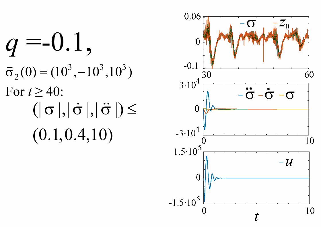
q =-0.1 3 3 3
2 (0) (10 , 10 ,10 )s = -r For t ≥ 40:
(| |,| |,| |)(0.1,0.4,10)
s s s £& &&

58
q = -1/3 SMC, no noise, 510-t =
(0) ( 100,100,100)z = - ,
2 (0) (10, 10,10)s = -r For t ≥ 30:
8 5 2
(| |,| |,| |)(4 10 ,2.2 10 ,2.7 10 )- - -
s s s £
× × ×
& &&

59
SMC: noise and differentiator 1 2 3, ( ) ( ) ( ) ( )ˆ t t t ts = s + h + h + hh = h , 510-t =
12
26
3 6 1/2
4 7
(0,0.2 )
sin(2 10 )00
10 c s
.2
o
1| cos( 1
)
) |
(10
N
tt
th =
h Î
×h =
×
35max(2 0.1 ,1) 0.35cos(1111 ), 0.2L t t M= - + = 2 (0) (10, 10,10)s = -
r , (0) ( 100,100,100)z = -

60
q = -1/3 SMC, noise, 510-t =
(0) ( 100,100,100)z = - ,
2 (0) (10, 10,10)s = -r For t ≥ 30:
(| |,| |,| |)(0.89,0.4,2.9)
s s s £& &&

61
Thank you very much!
Health to everybody

62
Appendices

63
Asymptotically optimal differentiation 0( ) ( ) ( )f t f t t= + h , | |h £ e, ( 1)
0| ( ) |dnf t L+ £ The worst-case error is not better (Levant, Yu, 2017) than
1
1 1 1
0
( )0inf sup | ( ) ( ) | 2 .
n ii i dn n nd d di
if tz t f t L
+ -+ + +- ³ e
(the Kolmogorov asymptotics) A differentiator is called asymptotically optimal, if for any 0( ) ( ) ( )f t f t t= + h , | |h £ e,
( )1 1
1 1 1( )0| ( ) ( ) |
n ii d n idn nd d ndi
i i i Lz t f t L L+ - + -
+ + +e£ g e g=-

64
Filippov Procedure
x& = f(x) Û x& Î KF[f](x) x(t) is an absolutely continuous function
0 0[ ]( ) convex_closure ( ( ) \ )F
NK f x f O x Ne
e> m == ∩ ∩
Non-autonomous case: 1t =& is added.
( ) 11 1
( ) 11 1
is understo)
[ , ] || || [ , ] ( )
[ |o, ] | || [ , ]
d[ ](
as
n nqn h m M n
n nqn h m M F n
C C K K u
C C K K K u
+- -
+- -
s Î - s + s
s Î - s + s
r r
r r