Embed Size (px)
Citation preview
www.imstat.org/aihp
Annales de l’Institut Henri Poincaré - Probabilités et Statistiques2011, Vol. 47, No. 3, 875–916DOI: 10.1214/10-AIHP391© Association des Publications de l’Institut Henri Poincaré, 2011
(Homogeneous) Markovian bridges
Vincent Vigon
IRMA, Université de Strasbourg. E-mail: [email protected]
Received 31 March 2009; revised 16 September 2010; accepted 28 September 2010
Abstract. (Homogeneous) Markov bridges are (time homogeneous) Markov chains which begin at a given point and end at a givenpoint. The price to pay for preserving the homogeneity is to work with processes with a random life-span.
Bridges are studied both for themselves and for their use in describing the transformations of Markov chains: restriction ona random interval, time reversal, time change, various conditionings comprising the confinement in some part of the state space.
These bridges lead us to look at Markov chains from an unusual point of view: we will work, no longer with only one transitionmatrix, but with a class of matrices which can be deduced one from the other by Doob transformations. This way of proceedinghas the advantage of better describing the “past ↔ future symmetries”: The symmetry of conditional independence (well known)and the symmetry of homogeneity (less well known).
Résumé. Les ponts markoviens (homogènes) sont des chaines de Markov (homogènes) qui démarrent à un point donné et meurentà un point donné. Pour préserver l’homogénéité, une telle chaine de Markov a nécessairement une durée de vie aléatoire.
Nous étudions les ponts pour eux mêmes et pour leur utilité à décrire les transformations d’une chaine de Markov : restrictionà un intervalle aléatoire, renversement temporel, changement de temps, conditonnements variés : notament le confinement dansune partie de l’espace d’état.
Ces ponts nous conduisent à considérer les chaines de Markov d’un point de vue inhabituel : nous ne travaillons plus avecune seule matrice de transition comme à l’accoutumée, mais avec une classe de matrices qui se déduisent les unes des autres partransformation de Doob. Cette méthode a l’avantage de mieux décrire les symétries passé ↔ futur : symétrie de l’indépendanceconditionnelle (bien connue) et symétrie de l’homogénéité (moins bien connue).
MSC: 60J10; 60J45; 47A68; 15A23; 60J50
Keywords: Markov chains; Random walks; LU-factorization; Path-decomposition; Fluctuation theory; Probabilistic potential theory; Infinitematrices; Martin boundary
0. Introduction
0.1. Motivations
To start with, let us enumerate some transformations of (good) Markov processes:
• The translation of the origin to a stopping time which preserves the law of the process up to a change of the initialdistribution (strong Markov property).
• The translation of the origin at the “splitting times” introduced by Jacobsen [18]. This family of times containsstopping times, return times, co-terminal times. As a remarkable example, the global minimizer of a trajectory isa splitting time (see Millar [24]).
• The killing of the trajectory at a splitting time which is the symmetric transformation of the previous one.• The confinement of trajectories to a part of the state space by conditioning. Such confinement, mixed with some
specific translation or killing, preserves the Markovian character of the process (see Jacobsen–Pitman [19]).
876 V. Vigon
• The time reversal (see e.g. Nagasawa [25]) which preserves the Markovian character (and which emphasizes thepast–future symmetry).
• The time change (or subordination) which allows us to restrict processes to some interesting random closed set (e.g.the left minima of Lévy processes, see Bertoin [1], Chapter 7). Subordination also allows us to compare Markovprocesses (see Simon [30]).
• The restriction of the trajectory to the complementary of a regenerative set which leads to the Itô [17] excursiontheory.
To describe the law of transformed Markov processes many authors use bridges, the most famous one being theBrownian bridge. For example Markovian bridges with deterministic life-spans are used by Getoor and Sharpe [13] todescribe excursions outside a regenerative set (i.e. set of type {t : Xt ∈ A}), while Fitzsimmons [8], for the same pur-pose, used bridges with random life-spans which have the advantage of being homogeneous Markov processes. Thesesame homogeneous bridges were used by Fourati [11] to generalize the Veervat [32] transform from the Browniancase to the more general Lévy processes case. We think that homogeneous bridges are a powerful tool, perhaps notwell enough known.
Most of the results appearing in the articles previously cited are profound and rather hard to establish. One of thegreat difficulties comes from the continuous time setting. Discrete Markov chains, which will occupy us, are reallymuch easier to work with. Meanwhile, the presented results offer a taste of the corresponding results for Markovprocesses. Homogeneous bridges will be our leading thread: we will study them for themselves and will explain howthey are usuful for understanding the transformations of Markov chains. Technically, it is more practical to considerethe family of bridges indexed by all the possible beginnings and ends. Such families will be called Markov-bridge-kernels.
0.2. Detailed summary
The global scheme of this article is the following: Section 1: Markov-bridge-kernels are defined by axioms. Section 2:We define the class of matrices which will parametrize Markov-bridge-kernels (just as transition matrices parametrizeMarkov chains). Section 3: We construct Markov-bridge-kernels by Doob transformations. Sections 4–9: We showhow bridges interact with classical Markov chains. Sections 10–12: We extend the definition of bridges in differentdirections. Sections 13–14: We ask some questions about existence and unicity relative to bridges.
We will now write summaries of each section. To keep them as short as possible, we will skip some hypothesesand bibliographic comments. All of these will be specified in the body of the text.
A trajectory ω ∈ Ω is a function from N to F = E ∪ {†} such that ωt = † ⇒ ωt+1 = †. Probabilities on Ω aredenoted by E or E{X ∈ •} (X being the canonical process i.e. the identity on Ω). Expectations are denoted by E[f]or E[f(X)] (brackets allow the distinction). For example, the law under E of the canonical process killed at a randomtime T is denoted by E{X[0,T ] ∈ •} = E[1{X[0,T ]∈•}].
Section 1: Parallel definition of Markov chains and Markov bridgesFrom an axiomatic point of view, a Markov-bridge-kernel is a family E•�• = (Ex�z)x,z∈E of probabilities on the setof trajectories such that, almost-surely under Ex�z, the canonical process begins at x and ends at z at a random time ζ ,and such that:
Ex�z
[∑t
f(X[0,t])1{Xt=y}g(X[t,ζ ])]
= Ex�y
[f(X)
]Ex�z
[∑t
1{Xt=y}]
Ey�z
[g(X)
],
where f,g are any test functions on Ω . Remark: in the left and right factors of the second line, the t disappears, whichis the sign of the time homogeneity. The above formula, called past–future extraction is the formula that makes bridgesso practical and beautiful.
(Homogeneous) Markovian bridges 877
To understand this past–future extraction, let us consider E• = (Ex)x∈E a transient Markov-chain-kernel whichis simply the law of a transient Markov chain started from all possible x ∈ E. The Markov property, summed at alltimes t gives:
Ex
[∑t
f(X[0,t])1{Xt=y}g(X[t,ζ ])]
= Ex
[∑t
f(X[0,t])1{Xt=y}]
Ey
[g(X)
].
The past–future extraction can be seen as a symmetrization of the above formula. Comparing the two previous formu-lae, we can see that a Markov-bridge-kernel E•�• is a family of Markov-chain-kernels (E•�z)z∈E , but this family iscoherent and the two indices x, z play a symmetric role.
Anticipating Section 5, Ex�z, can be interpreted as the law of X under Ex , killed the last time it visits z. But wewill not adopt this technique to construct Markov-bridge-kernels. Following Doob [5], and Fitzsimmons [8], we willuse Doob transformations.
Section 2: Matrices and their Doob classesA Markov chain is described by its starting point x and its transition matrix P . Henceforth, Markov-chain-kernelswill now be denoted by EP• = (EP
x )x∈E . A Markov-bridge-kernel is more naturally described by a transient D-classof matrices:
Let P be a non-negative matrix (i.e. a matrix with non-negative entries) and let U := ∑n P n be its potential matrix.
P is said to be transient if there exists g > 0 satisfying U[P ]g < ∞. The transience is stable by transposition.Let h > 0 be a function. The Doob transform of P is DhP(x, y) = h(y)
h(x)P (x, y). The D-class of P is DP =
{DhP : h > 0}. We see that P is transient if and only if any matrix of DP is transient.We also give some foundations for discrete potential theory, describing excessive functions (h ≥ 0,Ph ≤ h), in-
variant functions (h ≥ 0,Ph = h), and potential functions h = Ug,g ≥ 0. To excessive functions, we also associatea Doob transform DhP which is simply DhP restricted to the set where h is positive. It is immediate that DhP issub-stochastic.
From now on, our basic data will be a non-negative matrix P , or equivalently a D-class DP with a chosen repre-sentative P . Troughout the article, except in Section 12, P will be assumed transient. Each time we have to write EP
x ,we also require that P be sub-stochastic, but the bridge itself is defined for any transient P . This allows us to replaceP by P at any moment (doing this, we play with the time reversal).
Section 3: Construction of Markov-bridge-kernelsThe function U(•, z) = ∑
n P n(•, z) is P -excessive so the matrix P�z := DU(•,z)P is sub-stochastic. A Markov chaindriven by P�z dies at z with probability one. Moreover, for any h > 0, we have P�z = (DhP )�z. So we can denoteEP�z
x by EDPx�z. We establish the “past–future extraction” under EP
x i.e.
EPx
[∑t
f(X[0,t])1{Xt=y}g(X[t,ζ ])]
= EDPx�y
[f(X)
]EP
x
[∑t
f(X[0,t])]
EPy
[g(X)
].
We will use often this formula to describe transformations of Markov chains. Replacing EPx by EDP
x�z in the past–futureextraction shows that the constructed family EDP•�• is a Markov-bridge-kernel as defined in the axiomatic Section 1.
Section 4: Time reversalWe show that the law of the reversed path under the bridge i.e. EDP
x�z{(X ←[0,ζ ]) ∈ •} is equal to EDP
z�x {X ∈ •}. Note that
we have defined bridges for any transient matrix P (not necessarily sub-stochastic) so EDPz�x is well defined.
Section 5: Initial and final conditioningsProviding EP
x {∃t : Xt = z} > 0 we show that EDPx�z{X ∈ •} = EP
x {Xτz ∈ •/τz ∈ [0,∞[} where τz is the last visit at z.As a consequence, we show that any Markov chain that begins at x and ends at z has law EDP
x�z for a certain DP .
878 V. Vigon
Section 6: ConfinementLet A be a part of E × E representing some chosen transitions. Let {XX ⊂ A} be the event “all transitions of X
belong to A.” For example if E = N and A = {(x, y): x < y} then {XX ⊂ A} is “X increases.” Let SA be the first timewhere X makes a transition outside A. We explain the link between the conditioning by {XX ⊂ A}, the killing at SA
and making a final conditioning. For example we show that
EPx
{(X[0,SA])[0,τz] ∈ •/τz ∈ [0,∞[} = EDP
x�z
{X ∈ •/{XX ⊂ A}} = EDPA
x�z {X ∈ •},where PA(a, b) = P(a, b)1{(a,b)∈A}.
Section 7: Splitting trajectoryFollowing Jacobsen [18], we define splitting times as random times S such that, on {t ≤ ζ }, {S = t} = {X[0,t] ∈
CS}∩{X[t,ζ ] ∈ DS} where CS, DS are some subsets of Ω . Such splitting times generalize stopping times (the ones withDS = Ω) and return times (the ones with CS = Ω). An immediate consequence of the past–future extraction is that,under EP
x�z{X ∈ •/XS = y}, the pieces of trajectory X[0,S],X[S,ζ ] are independent and have laws EDPx�y{X ∈ •/DS}
and EDPy�z{X ∈ •/CS}.
Then we define “markers” which are families of times that generalize splitting times. These markers will be usedfurther on to describe excursions outside random sets.
Section 8: Time-change and excursionLet T be any stopping time taking values in [1, ζ ] ∪ {+∞}. We define the time-change � by iterating this stop-ping time: �0 = 0, �1 = T , . . . ,�n+1 = �n + T (X[�n,ζ ]). It is easy to verify that n �→ X�n
is also a Markov chainunder EP
x . Let us write �f the latest finite �n; using the past–future extraction we obtain:
EPx�z{X�f
= y}U(x, z) = EPx
[∑n
1{X�n=y}]
EPy
[∑t<T
1{Xt=z}]
=: VT (x, y)WT (y, z). (1)
Summing over all y we get the factorization U = VT WT which we will meet again further on.The set Λ = {t : ∃n: �n = t}, called past-spotted set, has some interesting properties and can be seen as a gen-
eralization of what is usually called a regenerative set. An excursion outside this set is a piece of trajectory of typeX[g,d] where ]g, d[ is a connected part of [0, ζ ] \ Λ. Each excursion which we can spot by events: before g, after d ,inside [g, d], or by intersections of three such events, can be described using the marker technique. We show that morecomplicated excursions cannot be described so easily.
Section 9: Fluctuation theoryThis theory is concerned with extrema of trajectories. The first minimizer ρ is a splitting time, and is also the end ofa past-spotted set. The associated factorization U = VT WT is then the classical LU-factorization, also called Wiener–Hopf factorization in the framework of random-walks. Bridges allow us to write an equivalent of the Veervat [32]transformation, namely:
EDPx�x
[f(X[ρ,ζ ] � X[0,ρ])/Xρ = y
] = EDPy�y
[f(X)/∃t : Xt = x,∀t Xt ≥ y
],
where � stands for the “biting” concatenation. Such a generalization of the Veervat transform has been made by Fourati[11] in the Lévy processes setting.
Section 10: Extension of the universeUntil now, we have worked on the canonical space which implies that all random elements are functions of X. In thissection we add an independent U[0,1] random variable which allows us to define randomized versions of splitting-time and time-change. For example the factorization (1) is still true when T is a randomized stopping time and�0,�1,�2, . . . are its randomized iterations.
We see also that an inequality P ≥ Q can be interpreted by the fact that the Q-Markov chain is equal to theP -Markov chain killed at a randomized stopping time. While U[P ] ≥ QU[P ] can be interpreted by the fact that theQ-Markov chain is equal to the P -Markov chain time-changed by a randomized time-change.
(Homogeneous) Markovian bridges 879
Section 11: Extension to the Martin boundaryIn this section we add the hypothesis that the graph of P is locally finite and irreducible. It is a common assumptionwhen constructing the Martin boundary. Roughly speaking, the minimal Martin boundary Mmin is the set of allpossible limits ξ for a Markov chain X driven by any one of sub-stochastic matrices Q ∈ DP . This Martin boundarycan also be identified with all the P -invariant minimal functions. It is very natural to extend the bridge (EDP
x�z)x,z∈E
to (EDPx�η)x∈E,η∈E∪Mmin .
We explain the link between confinement (as in Section 6) and final conditioning, but now “final conditioning” alsoincluded the conditioning by: “X reaches the Martin boundary at ξ ∈ Mmin” (in an infinite length of time).
Section 12: Un-normalized bridgesWhen P is sub-stochastic and transient, an expression for the bridge can be:
EDPx�y = EP
x [∑t 1{X[0,t]∈•}1{Xt=y}]U[P ](x, y)
,
the transience hypothesis ensuring U[P ](x, y) < ∞. Then we define the un-normalized bridge FPx�z as the numerator
of the above ratio. This notion extends to any P with finite spectral radius. We see that the past–future extraction andthe time-reversal formula are still valid. We compare advantages of normalized and un-normalized bridges.
Section 13: When two bridges partially coincideA set K ⊂ E is said to be P -closed when, in the directed graph of P , every trajectory which begins and ends in K ,lies entirely in K . E.g. P -absorbing sets are P -closed. Let K be a P -closed and P ′-closed set. Writing PK(x, y) :=P(x, y)1{x,y∈K} and DPK := D(PK) we have:
DPK = DP ′K ⇒ ∀x, z ∈ K EDP
x�z = EDP ′x�z.
Assuming the existence of some “directed-spanning-trees” in graphs of P,P ′, we show that the converse of thisimplication is also true. The existence of such a tree is always true if you suppose P,P ′ irreducible.
Applying this, we give a necessary and sufficient condition to have
EPx {X[0,t] ∈ •/Xt = z} = EP ′
x {X[0,t] ∈ •/Xt = z}.
Section 14: All axiomatic bridges can be constructedFor any Markov-bridge-kernel E•�• (in the sense of the axiomatic definition given in Section 1), we show that thereexists a D-class DP such that E•�• = EDP•�•.
Remark. Why we do not assume irreducibility? This assumption, which is almost necessary for recurrent theory,is not really appropriate for our subject because some killings, conditionings and time-changings do not keep theirreducible character. Moreover, Markov chains are sometimes called “random dynamic system.” To merit this name,we have to include cases where trajectories starting from different points do not necessarily intersect each other.
1. Parallel definition of Markov chains and Markov bridges
1.1. Definition of a Markov chain
Let F be a denumerable set. Elements of FN are called trajectories. The set FN is endowed with the cylindrical σ -field.We can restrict a trajectory: ω[0,t] = (ω0ω1 · · ·ωt), translate it: ω[t,∞[ = (ωtωt+1ωt+2 · · ·), mix the two operations:ω[t,t+s] = (ω[t,∞[)[0,s] = (ωtωt+1 · · ·ωt+s), and even reverse the time: ω←[0,t]
= ωtωt−1 · · ·ω0.
An inhomogeneous Markov chain is a random element X : (Ω, F ,E) �→ FN such that, for all t ∈ N, X[0,t] andX[t,∞[ are independent conditionally to Xt . A Markov chain is an inhomogeneous Markov chain which satisfiesmoreover ∀x ∈ F , ∀s, t ∈ N, E{X[s,∞[ ∈ •/Xs = x} = E{X[t,∞[ ∈ •/Xt = x}, whenever the two conditionings arewell defined.
880 V. Vigon
Our purpose is to give general considerations about Markov chains (and not to talk about a particular one, con-structed in a particular setting), so it is more convenient to work in the canonical framework: from now on, we considerX :FN �→ FN the identity application. A probability E on F N is a Markov-chain-law when, under E, X is a Markovchain. Actually, it is more practical to consider a family of Markov-chain-laws rather that one:
Definition 1.1. A Markov-chain-kernel E• = (Ex)x∈F is a family of probabilities on FN satisfying the followingaxioms:
1. “Support”: We have Ex{X0 = x} = 1 for all x ∈ F .2. “Markov property”: We have
Ex
[f(X[0,t])1{Xt=y}g(X[t,∞[)
] = Ex
[f(X[0,t])1{Xt=y}
]Ey
[g(X)
]for all states x, y ∈ F , times t ∈ N, test functions f :F [0,t] �→ R+ and g :FN �→ R+.
Clearly, when E• is a Markov-chain-kernel and when α is a probability on F then Eα := ∑a α(a)Ea is a Markov-
chain-law.Reciprocally, when E is a Markov-chain-law, then, for all x ∈ F , we can define: Ex := E{X[Tx,∞[ ∈ •/Tx < ∞}
where Tx = inf{t ≥ 0: Xt = x}, if the conditioning is well defined (and anything if not). The kernel (Ea)a∈F that wewent to construct is a Markov-chain-kernel and we have E = Eα with α = E{X0 ∈ •}.
1.2. Transient case
Now we distinguish a state † ∈ F , called cemetery point, and put E = F \ {†}. We denote by Ω the event {∀t : Xt =† ⇒ Xt+1 = †} (i.e. the event “† is absorbing”). On Ω we define the random time ζ = sup{t : Xt ∈ E}. Thus the event{ζ < ∞} ⊂ Ω represents all the trajectories that meet †. From now on, a restricted trajectory ω[0,t] is identified withω0ω1 · · ·ωt†† · · · so that
⋃s∈N E[0,s] ∪ EN is identified with Ω . As a consequence X[t,∞[ = X[t,ζ ].
Definition 1.2. A transient Markov-chain-kernel E• = (Ex)x∈E is a family of probabilities on FN satisfying the fol-lowing axioms:
1. “Support”: We have Ex{X0 = x ∩ Ω} = 1 for all x ∈ E.2. “Transience”: We have Ex[∑t 1{Xt∈K}] < ∞ for all x ∈ E and finite K ⊂ E.3. “Future extraction”: We have
Ex
[∑t
f(X[0,t])1{Xt=y}g(X[t,ζ ])]
= Ex
[∑t
f(X[0,t])1{Xt=y}]
Ey
[g(X)
]
for all states x, y ∈ E, and test functions f,g :Ω �→ R+.
Remark 1.3.
• In the above formula, the summation∑
t can be replaced by∑
t≤ζ thanks to the term 1{Xt=y} with y ∈ E.• The family E• = (Ex)x∈E can be extended to E• = (Ex)x∈F by setting E† to be the Dirac measure on the trajectory
††† · · · .• Let us consider any process t �→ Zt which is “past-adapted” i.e. ∀t Zt is σ(X[0,t])-measurable. Using the fact
that X[0,t] = X[0,t] ◦ X[0,t] we see that Zt = Zt(X[0,t]). Using the fact that, on {t ≤ ζ }, t = ζ ◦ X[0,t], we get:Zt1{t≤ζ } = (Zζ )(X[0,t])1{t≤ζ }. So processes of type t �→ f(X[0,t]) represent the most general class of past-adaptedprocess (whenever we work on the life interval [0, ζ ]).
• The future extraction is a reformulation of the Markov property (second axiom of Definition 1.1): you go from theMarkov property to the future extraction by summing over all t ∈ N. You go from the future extraction to the Markovproperty replacing f(X) by f(X)1{ζ=t}. So clearly a transient Markov-chain-kernel (Ex)x∈E is a Markov-chain-kernel.
(Homogeneous) Markovian bridges 881
Definition 1.4. A mortal Markov-chain-kernel E• = (Ex)x∈E is a family of probabilities on FN which satisfies ∀x ∈ E
Ex{X0 = x, ζ < ∞} = 1 and the axiom “future extraction” of Definition 1.2.
It is a classical exercise to check that a mortal Markov-chain-kernel also verifies the second axiom (transience) ofDefinition 1.2. So the mortality is a particular case of the transience.
1.3. Definition of a bridge
Definition 1.5. A Markov-bridge-kernel E•�• = (Ex�z)x,z∈E is a family of probabilities on FN satisfying the follow-ing axioms for all x, y, z ∈ E:
1. “Degeneracy”: If Ex�z{ζ = 0} = 1 then Ex�z is the Dirac measure on the trajectory x†† · · · . In this case we saythat Ex�z is degenerated.
2. “Support”: If Ex�z is non-degenerated then Ex�z{X0 = x,Xζ = z, ζ < ∞} = 1.3. “Cohesion”: If Ex�y,Ey�z are non-degenerated then Ex�z{∃t : Xt = y} > 0.4. “Past-future extraction”: We have
Ex�z
[∑t
f(X[0,t])1{Xt=y}g(X[t,ζ ])]
= Ex�y
[f(X)
]Ex�z
[∑t
1{Xt=y}]
Ey�z
[g(X)
]for all test functions f,g :Ω �→ R+.
Remark 1.6. The past–future extraction can be seen as a symmetrization of the future extraction. To see the symmetry,we can define (E
x�z)x,z∈E by Ex�z = Ez�x{(X ←[0,ζ ]
) ∈ •} when Ez�x is non-degenerated, and Ex�z = δx††··· when
Ez�x is degenerated. The reader is invited to check that this new family E•�• is a Markov-bridge-kernel.
Remark 1.7. The axiom “support” is partially included in the axiom “past–future extraction”: If you weaken “sup-port” by: “If Ex�z is not degenerated then Ex�z{∃t : Xt = x} > 0, Ex�z{∃t : Xt = z} > 0” then, applying “past–futureextraction” with f := 1{Xζ =z}, y := z,g := 1Ω gives you Ex�z{Xζ = z} = 1 while applying “past–future extraction”with f := 1Ω,y := x,g := 1{X0=x} gives you Ex�z{X0 = x} = 1.
Proposition 1.8 (Past and future extractions). Let E•�• be a Markov-bridge-kernel. For every states x, y ∈ E andtest functions f,g : Ω �→ R+ we have:
• The future extraction:
Ex�z
[∑t
f(X[0,t])1{Xt=y}g(X[t,ζ ])]
= Ex�z
[∑t
f(X[0,t])1{Xt=y}]
Ey�z
[g(X)
].
• The past extraction:
Ex�z
[∑t
f(X[0,t])1{Xt=y}g(X[t,ζ ])]
= Ex�y
[f(X)
]Ex�z
[∑t
1{Xt=y}g(X[t,ζ ])].
Proof. Applying the past–future extraction with the pair (f,1Ω) gives:
Ex�z
[∑t
f(X[0,t])1{Xt=y}]
= Ex�y
[f(X)
]Ex�z
[∑t
1{Xt=y}].
Substituing this equality in the past–future extraction with a pair (f,g) gives the future extraction. Past extraction isproven similarly. �
Corollary 1.9. Let E•�• be a Markov-bridge-kernel. For every z ∈ E, E•�z is a mortal Markov-chain-kernel.
Thus, a Markov-bridge-kernel may be considerated as a coherent family of Markov-chain-kernels.
882 V. Vigon
1.4. From Markov-chain-kernel to matrices
To a Markov-chain-kernel E•, we can associate its transition matrix ∀x, y ∈ F P(x, y) := Ex{X1 = y} which isstochastic i.e.
∑a∈F P (x, a) = 1. Reciprocally, to each stochastic matrix corresponds a unique Markov-chain-kernel
as explained below:Let P be any stochastic matrix on F . For each x ∈ F , there exists a unique probability EP
x satisfying
EPx {X0 = x0,X1 = x1, . . . ,Xn = xn} = δx(x0)P (x0, x1) · · ·P(xn−1, xn)
for all times t ∈ N and families of states x0, . . . , xn ∈ F . (The unicity comes from the monotone class theorem, theexistence from the Kolmogorov theorem.) The family EP• constructed by this way is a Markov-chain-kernel whosetransition matrix is P .
A Markov-chain-kernel EP• supported by Ω is also characterized by the restriction of its transition matrix to E.Indeed, once we get P := P |E , we can reconstruct P on F by P(x,†) = 1 − ∑
y∈E P (x, y) and P(†,†) = 1. Inthis case, we will prefer to write EP• instead of EP• . Remark also that the restricted matrix P is sub-stochastic i.e.∀x
∑y P (x, y) ≤ 1.
From now on, it is clear that the data of a sub-stochastic matrix P on E or a Markov-chain-kernel EP• supportedby Ω are equivalent. We prefer to use the matrix as our first data.
2. Matrices and their Doob classes
The main purpose of this section is to introduce and study the “transient D-classes of matrices” which will parametrizebridges.
Data 2.1. Throughout this article, P will represent a non-negative matrix indexed by E (non-negative means ∀x, y ∈E P(x, y) ≥ 0). Assumptions of transience (see below), sub-stochasticity and irreducibility will be added further on.
2.1. Notations
By default, functions f,g,h, measures α,β,μ, ν and matrices P,Q, are defined on E or E ×E and take values in R+(never in R+ ∪ {+∞}). We write briefly h > 0 to indicate that the function h is everywhere positive. The differencebetween a function and a measure is purely of a lexical order. The destiny of functions is to be multiplied on the leftof matrices, and so they can be drawn as column vectors. The destiny of measures is to be multiplied on the right ofmatrices, and so they can be drawn as row vectors. E.g.
μP(y) =∑a
μ(a)P (a, y), Ph(x) =∑
b
P (x, b)h(x).
In this paper, a directed graph (B,→) is the data of a denumerable set B (often B = E) and a relation → betweenelements of B . A vertex b is an element of B , an directed edge (a → c) is a related pair of vertices. For example, the
directed graph P is (E,P→) with a
P→ c ⇔ P(a, c) > 0.We write a � c when there exists an directed chain a → b1 → ·· · → bn → c. We accept degenerated chains, so
we always have a � a. For example, when P is sub-stochastic: aP� c ⇔ EP
a {∃t : Xt = c} > 0.For A,C sets of vertices, we write {• � C} = {b: ∃c ∈ C: b � c}, {A � •} = {b: ∃a ∈ A: a � b}, and {A � • �
C} = {b: ∃a ∈ A,∃c ∈ C: a � b � c}.Because P will come back very often, we will sometimes drop the mention of P in sentences like: “Let h be
a P -excessive function. . . .” We also leave out P in many notations like “U[P ]” (the potential matrix relative to P ) or“x
P� y.”
(Homogeneous) Markovian bridges 883
2.2. Transient and mortal matrices
We denote by:
U[P ](x, y) =∑
t
P t (x, y) ∈ [0,∞[, where P 0 = I is identity.
U[P ] is called the potential matrix associated to P .
Definition 2.2 (Transience). A weighting function for P if a function g > 0 such that ∀x ∈ E: U[P ]g(x) < ∞. Wesay that P is transient if such a weighting function exists for P . Transient matrices are matrices with spectral radiusa bit less than one, in a sense we will explain in Section 12.1.
We insist on the fact that, for us, a transient matrix is not necessarily sub-stochastic; however in this case, we havea nice characterization of transient matrices:
Proposition 2.3. Suppose that P is sub-stochastic. The following points are equivalent:
1. P is transient.2. For all x, y ∈ E, U[P ](x, y) < ∞.3. The Markov-chain-kernel EP• is transient.
Proof. 1 ⇒ 2 is obvious.2 ⇔ 3 comes from the fact that we can interpret U[P ](x, y) as EP
x [∑t 1{Xt=y}].3 ⇒ 1. Applying the Markov property at time Ta = inf{t : Xt = a} gives:
U(x,a) = EPx
[∑t≥Ta
1{Xt=a}]
= EPx {Ta < ∞}U(a,a)
so that U(•,a)U(a,a)
is bounded by 1. Pick a probability α > 0 and set g(a) = α(a)U(a,a)
> 0. Therefore we obtain Ug ≤ 1, so g
is a weighting function for P . �
Proposition 2.4. P is transient if and only if P is transient.
Proof. Let g be a weighting function for P . We have Ug ≥ g > 0. We take a probability α > 0. We define the measureμ(x) = α(x)
Ug(x). Then we have μUg = 1, so ∀x μU(x) is finite and μ can be taken as a weighting function for P .
�
We appreciate the transience because of its stability under transposition (which is not the case for the sub-stochasticity). In particular, working with such matrices avoids having to make different statements for excessivefunctions and excessive measures.
Definition 2.5 (Mortality). We say that P is mortal when it is sub-stochastic and when moreover ∀x ∈ E:limn P n1E(x) = 0.
Because P n1E(x) = EPx {ζ ≥ n}, the mortality of P is equivalent to the mortality of EP• . So the mortal matrices are
sub-stochastic and transient. We can compare mortal matrices with the stochastic ones, which could also be qualifiedof immortal.
2.3. Excessive, invariant, potential functions
A function h ≥ 0 is said to be: P -excessive if Ph ≤ h, P -invariant if Ph = h, P -potential if there exists a functiong ≥ 0, called the charge, such that h = U[P ]g. A (non-negative) measure μ is said to be P -excessive, P -invariant,P -potential if its transposition μ is P -excessive, P -invariant, P -potential.
884 V. Vigon
An excessive function h is a potential function if and only if P nh tends to 0 point-wise. The Riesz decompositionsays that every excessive function can be written as the sum of an invariant function and a potential one. For moredetails about this subject see e.g. Dellacherie–Meyer [4].
2.4. Doob transformations
For any h > 0 we note DhP(x, y) = h(y)h(x)
P (x, y). The application P �→ DhP is invertible and we easily check thatU[DhP ] = DhU[P ].
When h is a P -excessive function (which might vanish), we write:
DhP (x, y) = 1{h(x)>0}h(y)
h(x)P (x, y)
= h(y)P (x, y)
h(x)with the convention
0
0= 0.
The equality between the two lines comes from the fact that Ph ≤ h imposes h(x) = 0 ⇒ h(y)P (x, y) = 0.If you prefer to add the assumption that P is irreducible, then all excessive functions are everywhere positive, and
you can replace D by D.
Proposition 2.6. Let h be a function everywhere positive. We have:
• DhP is sub-stochastic if and only if h is P -excessive.• DhP is sub-stochastic and mortal if and only if h is P -potential.• DhP is stochastic if and only if h is P -invariant.
The proof is easy and left to the reader.
2.5. Doob classes (D-classes)
Let P ′,P ′′ be two non-negative matrices. We say that they are D-equivalent if there exists a function h > 0 such thatP ′′ = DhP
′. The equivalence class of P is denoted by DP . If P is transient, then, all matrices of DP are transient(because U[DhP ] = DhU[P ]).
As we will see in the proof of the following proposition, properties relative to a transient matrix P can be oftenproved using a sub-stochastic matrix P ′ in DP .
Proposition 2.7. P is transient if and only if there exists a function h > 0 which is P -potential.
Proof. Suppose P transient. Let g > 0 be a weighting function for P . Then the function h = U[P ]g is potential andeverywhere positive.
Conversely, suppose the existence of a function h = U[P ]f > 0. We set P ′ = DhP which is sub-stochastic. Thetransience of P is equivalent to the transience of P ′. We also remark that 1E = U[P ′] f
h.
We pick q ∈ ]0,1[. The quantity g(x) = U[P ′](U[qP ′] fh)(x) = U[qP ′]1E(x) ≤ 1
1−qis everywhere finite. In order to
use g as a weighting function for P , it remains to prove the positivity of g.Let T = inf{t : Xt ∈ {f
h> 0}} = inf{t : Xt ∈ {f > 0}}. The positivity of U[P ′] f
h(x) implies (and is equivalent to)
EP ′x {T < ∞} > 0. So, denoting by μx the sub-probability on N defined by μx(t) = EP ′
x {T = t}, this sub-probability isnon-identically zero. On another hand, the positivity of U[qP ′] f
h(x) is equivalent to the positivity of EP ′
x [qT 1{T <∞}] =∑t q
tμx(t) which is true because the function t �→ qt is everywhere positive on N. �
Corollary 2.8. P is transient if and only if, among matrices of DP , there exists a least one matrix which is sub-stochastic and mortal.
(Homogeneous) Markovian bridges 885
Proof. Suppose P transient. Let g be a weighting function for P . Put h = Ug > 0 and Q = DhP ∈ DP . Becauseh is a P -potential function, Q is sub-stochastic and mortal. Reciprocally, suppose that there exists Q in DP whichis mortal and sub-stochastic. But because Q is mortal, from Proposition 2.6, h is P -potential. From Proposition 2.7,P is transient. �
Remark 2.9. At this point comes a natural question: when P is transient, does there exist a matrix Q in DP whichis stochastic, or equivalently: does there exist a P -invariant function h > 0? When P is irreducible the necessarya sufficient condition is that E is infinite: it is a consequence of the Martin Boundary theory and this will be explainedin Section 11. For a reducible matrix, the natural condition would be the existence, for each state x, of an infinite pathstarting from x and leaving every finite subset of E. But we do not find a reference for this. . . .
2.6. Absorbing sets
A set K ⊂ E is said absorbing when K = {K P� •}. Every set of the form {A P� •} are P -absorbing.A short analysis shows us that K is P -absorbing if and only if 1K is a P -excessive function. Moreover, the support
of any P -excessive function is P -absorbing. For a P -potential function h = Ug we have {h > 0} = {• P� {g > 0}}.Looking at the definition of the transformation D, we see that the graph of DhP is the restriction of the graph of
P to {h > 0}. In particular the graph of DU(•,z)P is the restriction of the graph of P to {• P� z}. In the next section,we will see how such a matrix DU(•,z)P allows us to construct the bridge ending at z.
3. Construction of Markov-bridge-kernels
The use of Doob transformations to produce Markovian trajectories ending at one specified point, comes back toDoob [5]. The idea of considering homogeneous bridges as a whole family for describing some pieces of trajectoryis due to Fitzsimmons [8]. The notion of bridges we develop here is the normalized and discrete version of the onedeveloped by Fitzsimmons.
Data 3.1. From now on, P is a transient matrix.
3.1. A killing
Lemma 3.2. Let Q be a sub-stochastic matrix. We have EQx {Xζ = y} = U[Q](x, y)Q(y,†) with Q(y,†) = 1 −∑
a Q(y, a).
Proof. EQx {Xζ = y} = EQ
x
∑t 1{Xt=y}1{Xt+1=†} = U[Q](x, y)Q(y,†). �
Proposition 3.3. Let U[P ]g = Ug be a P -potential function. The Markov-chain-kernel EDUgP• is mortal and satisfies:
∀x, y ∈ E EDUgPx {Xζ = y} = U[P ](x, y)g(y)
U[P ]g(y)with
0
0= 0.
Proof. The mortality of DUgP (⇔ the mortality of EDUgP• ) comes from the fact that Ug is a potential function. Let
us compute the law of the position at ζ . From the previous lemma, we need to compute DUgP (x,†). We make thenext computation, using the convention 0
0 = 0:
DUgP (x,†) = 1 −∑a
Ug(a)
Ug(x)P (x, a) = 1 − PUg(x)
Ug(x)= 1 − Ug(x) − g(x)
Ug(x)= g(x)
Ug(x).
From the previous lemma: EDUgPx {Xζ = y} = U[DUgP ](x, y)
g(y)Ug(y)
= U(x,y)g(y)Ug(y)
. �
886 V. Vigon
3.2. A candidate for the bridge
For any transient matrix Q we write Q�z for DU[Q](•,z)Q.
Lemma 3.4 (Fundamental). Fix z ∈ E. For any function h > 0 we have (DhP )�z = P�z. For any P -excessivefunction h ≥ 0 such that z ∈ {h > 0} we have (DhP )�z = P�z.
Proof. We write P ′ = DhP and U ′ = U[P ′]. Clearly {U(•, z) > 0} = {U ′(•, z) > 0}. When a, b belong to this set:
P ′�z(a, b) = U ′(b, z)
U ′(a, z)P ′(a, b) = (h(z)/h(b))U(b, z)
(h(z)/h(a))U(a, z)
h(b)
h(a)P (a, b) = P�z(a, b), (2)
when a or b does not belong to this set then clearly P ′�z(a, b) = P�z(a, b) = 0.
Suppose now that P ′ = DhP with h excessive and z ∈ {h > 0}. Because {h > 0} is P -absorbing we have {h >
0} ⊃ {• P� z}. In particular {U(•, z) > 0} = {U ′(•, z) > 0}. The rest of the proof is similar. �
If x �� z then P�z(x, z) = 0 so that EP�zx is the Dirac measure on the trajectory x†† · · · . If x � z then Propo-
sition 3.3 indicates that EP�zx {Xζ = y} = I (y, z). So the family (EP�z
x )x,z∈E is the good candidate to be a Markov-bridge-kernel.
On the other hand, the first part of the fundamental Lemma 3.4 says that: if P ′ is a matrix of DP , then P ′�z = P�z.
This allows us to state:
EDPx�z := EP�z
x = EP ′�zx .
This notation emphasizes that EDPx�z is a function of the class DP . This notation also emphasizes a symmetry between
the initial point x and the final point z.
3.3. Past–future extraction
The following theorem gives formulae which explain the appearance of EDPx�z appear in many contexts (see Section 7
for concrete applications). Moreover, these formulae will say that EDP•�• is a Markov-bridge-kernel as defined in theaxiomatic Definition 1.5.
Theorem 3.5. We fix f,g :Ω �→ R+ and x, y, z ∈ E.
1. Suppose that P is sub-stochastic and transient. EPx satisfies the past–future extraction property i.e.:
EPx
[∑t
f(X[0,t])1{Xt=y}g(X[t,ζ ])]
= EDPx�y
[f(X)
]EP
x
[∑t
1{Xt=y}]
EPy
[g(X)
]= EDP
x�y
[f(X)
]U(x, y)EP
y
[g(X)
].
2. Suppose that P is just transient. EDPx�z satisfies the past–future extraction property i.e.:
EDPx�z
[∑t
f(X[0,t])1{Xt=y}g(X[t,ζ ])]
= EDPx�y
[f(X)
]EDP
x�z
[∑t
1{Xt=y}]
EDPy�z
[g(X)
]
= EDPx�y
[f(X)
]U(x, y)U(y, z)
U(x, z)EDP
y�z
[g(X)
](with the convention 0
0 = 0).
(Homogeneous) Markovian bridges 887
Proof. 1. If x �� y then the equation becomes 0 = 0. We assume now that x � y. Applying the Markov property ateach t (or the “future extraction”):
EPx
[∑t
f(X[0,t])1{Xt=y}g(X[t,ζ ])]
= EPx
[∑t
f(X[0,t])1{Xt=y}]
EPy
[g(X)
].
So, to prove the past–future extraction it is sufficient to establish:
EPx
[∑t
f(X[0,t])1{Xt=y}]
= EDPx�y
[f(X)
]U(x, y). (3)
By monotone class theorem, it is sufficient to establish this equality for all functions of type f = 1{X0=x0,...,Xn=xn}.Replacing f in the left-hand side of (3) gives:
EPx
[∑t
1{X0=x0,...,Xn=xn}1{Xt=y}]
=∑t≥n
I (x, x0)P (x0, x1) · · ·P(xn−1, xn)Pt−n(xn, y)
= I (x, x0)P (x0, x1) · · ·P(xn−1, xn)U(xn, y).
Replacing f in the right-hand side of (3) gives:
EDPx�y
[f(X)
]U(x, y) = I (x, x0)P�y(x0, x1) · · ·P�y(xn−1, xn)U(x, y).
To identify, we just have to recall that P�y = DU(•,y)P .2. We can apply the first part of this theorem, substituting P by P�z (which is sub-stochastic):
EP�zx
[∑t
f(X[0,t])1{Xt=y}g(X[t,ζ ])]
= EDPx�y
[f(X)
]U[P�z](x, y)EP�z
y
[g(X)
].
But we have U[P�z](x, y) = U(x,y)U(y,z)U(x,z)
, with 00 = 0. �
Corollary 3.6. The family EDP• = (EDPx�z)x,z∈E is a Markov-bridge-kernel in the sense of Definition 1.5.
Remark 3.7. Let h ≥ 0 be a P -excessive function. Using the second part of the fundamental Lemma 3.4, we see thatthe past extraction can be applied to DhP as follows
∀x ∈ {h > 0} EDhPx
[∑t
f(X[0,t])1{Xt=y}]
= EDPx�y
[f(X)
]DhU(x, y)
while the previous theorem gives us only ED(DhP )x�y [f(X)]DhU(x, y).
4. Time reversal
Data 4.1. From now on, P is a transient and sub-stochastic matrix.
Here is a very old question: At what kind of times can a Markov chain be reversed to produce a Markov chain?More precisely: for which L :Ω �→ N ∪ {��} (�� is a refuge) is EP
α {X ←[0,L]∈ •/L �= ��} still a Markov chain law? Let
us call such times L “reversers.”
888 V. Vigon
Kolmogorov [21] explained that a Markov chain started with an invariant distribution can be reversed at a deter-ministic time t to produce a t -steps Markov chain (i.e. a chain killed at t ). But remark that a Markov chain killed ata deterministic time is inhomogeneous, so deterministic times are not reversers.
Hunt [15] shows that last entrance times are reversers. Nagasawa [25], in a continuous-time setting, shows that“return times” (see Section 7.1) are reversers. Proposition 4.2 below is a discrete time version of Nagasawa’s theorem.
But the more synthetic answer is: Reversers are random times L such that X[0,L] is a Markov chain: The actionof reversing the time is completely inoffensive for Markov chains. The real danger is the killing! So a better term forreversers is: “death times,” and the most general class of such times has been described by Jacobsen (see Section 7.2).It is worth noting that there is death times (and so reversers) that are not return times; so the terminology “returntimes” is a bit of an overstatement.
In this section, we consider mortal Markov chains, so we are not really preoccupied by the killing. We see how thetransition matrix is changed by time reversal, and we see how this becomes simple when the mortal Markov chain isa bridge.
4.1. To reverse a mortal Markov chain
Proposition 4.2. Let α be a probability on E. Denote by P = DαUP and by β = EPα {Xζ = y}. We have:
EPα {X ←[0,ζ ]
∈ •} = EPβ {X ∈ •}.
Proof. It is enough to test this equality with cylindrical functions f = 1{X0=y0,...,Xn=yn}:
EPα
[f(X ←[0,ζ ]
)]
=∑t≥n
EPα {ζ = t,Xt = y0,Xt−1 = y1, . . . ,Xt−n+1 = yn−1,Xt−n = yn}
=∑t≥n
EPα {Xt−n = yn,Xt−n+1 = yn−1, . . . ,Xt−1 = y1,Xt = y0,Xt+1=†}
=∑t≥n
αP t−n(yn)P (yn, yn−1) · · ·P(y1, y0)P (y0,†)
= P(y0,†)P (y0, y1) · · ·P (yn−1, yn)αU(yn)
= αU(y0)P (y0,†)DαUP (y0, y1) · · · DαUP (yn−1, yn)
= β(y0)P (y0, y1) · · · P (yn−1, yn),
to make β appear in the last line, we used Lemma 3.2. �
4.2. To reverse a bridge
Theorem 4.3. Suppose xP� z. We have:
EDPx�z{X ←[0,ζ ]
∈ •} = EDPz�x {X ∈ •}.
Proof. Let us consider the probability EDPx�z{X ←[0,ζ ]
∈ •} = EP�zx {X ←[0,ζ ]
∈ •}. According to the previous lemma, it is a
Markov chain whose initial law is δz and whose transition matrix is:
P = DδxU[P�z](P�z) = (
P )�x
.
So that EDPx�z{X ←[0,ζ ]
∈ •} = EDPz�x {X ∈ •}. �
(Homogeneous) Markovian bridges 889
5. Initial and final conditionings
We give a recipe to produce a bridge by mixing a killing and a conditionning.
5.1. Notations
We denote by Ty = inf{t : Xt = y}. We call initial conditioning the transformation from E{X ∈ •} into E{X[Ty,ζ ] ∈•/Ty < ∞} which is written symbolically by an arrow as follows:
E{X ∈ •} y�−−−−−→ E{X[Ty,ζ ] ∈ •/Ty < ∞}.
If we apply this transformation to EPx (assuming x � y) then the strong Markov property applied to Ty gives imme-
diately EPx
y�−→ EPy .
Symmetrically, we denote by τy = sup{t : Xt = y}. We call final conditioning the transformation from E{X ∈ •}into E{X[0,τy ] ∈ •/τy ∈ [0,∞[} which is written symbolically:
E{X ∈ •} �y−−−−−→ E{X[0,τy ] ∈ •/τy ∈ [0,∞[}.
5.2. Final conditioning produces a bridge
Theorem 5.1.
1. Suppose x � y. The final conditioning transforms a Markov chain into a bridge:
EPx
�y−−−−−→ EDPx�y.
2. Suppose x � y � z. The final conditioning transforms a bridge into another bridge:
EDPx�z
�y−−−−−→ EDPx�y.
3. Suppose x � y � z. The initial conditioning transforms a bridge into another bridge:
EDPx�z
y�−−−−−→ EDPy�z.
Proof. 1. We have {τy ∈ [0,∞[} = {Ty < ∞} = {∃t : Xt = y} and in virtue of our hypothesis x � y, this event asnon-zero probability under EP
x . Applying the past–future extraction (Theorem 3.5, item 1) gives:
EPx
[f(X[0,τy ])1{∃tXt=y}
] = EPx
[∑t
f(X[0,t])1{Xt=y}1{∀s≥1,Xs �=y} ◦ X[t,ζ ]]
= EDPx�y
[f(X)
]U(x, y)EP
y {∀s ≥ 1,Xs �= y}.Denote R(f) the quantity above. Computing R(f)/R(1Ω) gives the first point of the theorem. The second comes bydoing the same calculus, but starting from EP
x�z instead of EPx . The third point comes directly by applying the strong
Markov property at the time Ty under EDPx�z. �
Corollary 5.2. The initial and final conditioning commute:
EPx
a�−−−−−→ EPa
�b−−−−−→ EDPa�b,
EPx
�b−−−−−→ EDPx�b
a�−−−−−→ EDPa�b.
890 V. Vigon
5.3. Application: Characterizations of bridges
The following proposition indicates that a bridge is a just a Markov chain that dies at an unique point.
Proposition 5.3. Suppose x � z. The following points are equivalent:
1. EPx = EDP
x�z.
2. EPx {Xζ = z} = 1.
Proof. 1 ⇒ 2. Obvious.2 ⇒ 1. From Theorem 5.1 we know that final conditioning produces bridge i.e:
EDPx�z{X ∈ •} = EP
x
{X[0,τz] ∈ •/τz ∈ [0,∞[}
but point 2 implies that τz = ζ a.s. and EPx {τz ∈ [0,∞[} = 1, so the right-hand term of the above formula is equal to
EPx {X ∈ •}. �
Proposition 5.4. Let z be a fixed state. The following points are equivalent:
1. ∀x EPx = EDP
x�z.2. The function x �→ U[P ](x, z) is constant and P(z,†) = 1 − ∑
a P (z, a) > 0.3. The function x �→ EP
x {Xζ = z} is constant and non-zero.
4. The function x �→ EPx {Tz < ∞} is constant and non-zero.
When it is the case, the two last functions are equal to 1.
Proof. If there exists a such that a �� z, then, all points 1, 2, 3 and 4 are false. So we can suppose without loss ofgenerality that E = {a :a � z}, so that the function a �→ U(a, z) is everywhere positive.
1 ⇒ 2. We see that 1 is also equivalent to P = P�z. We have:
∀x U[P ](x, z) = U[P�z](x, z) = DU(•,z)U(x, z) = U(z, z).
2 ⇔ 3. Comes directly from Lemma 3.2.2 ⇔ 4. Comes from the formula EP
x {Tz < ∞} = U(x,z)U(z,z)
.3 ⇒ 1. Suppose 3. We have:
EPx {Xζ = z} = EP
x {Tz < ∞,Xζ ◦ X[Tz,ζ ] = z} = EPx {Tz < ∞}EP
z {Tz < ∞}so the function x �→ EP
x {Tz < ∞} is necessarily equal to 1. This forces the canonical process to go into z from anystate. Because we have excluded the recurrent case (P is transient), we deduce that the canonical process necessarilydies at z with probability one. Thus ∀x EP
x = EPx�z. �
6. Confinement
6.1. Restriction of possible transitions
Let A be a subset of E ×E which represents some “selected transitions.” Pair of states will be often written xy insteadof (x, y). We define the following event:
{XX ⊂ A} := {∀t < ζ : XtXt+1 ∈ A}.For example, if K ⊂ E and A = K × K then {XX ⊂ A} means “X stays all its life inside K” and this event is alsodenoted by X ⊂ K . As a second example, if E = Z and A = {xy: x < y} then {XX ⊂ A} is the set trajectories thatincrease (until ζ ).
(Homogeneous) Markovian bridges 891
We denote by: PA(x, y) = P(x, y)1xy∈A and by SA = inf{t : XtXt+1 /∈ A}, so X[0,SA] belongs to {XX ⊂ A}. If Eis any probability supported by Ω , we define the following two transformations:
E{X ∈ •} X[0,SA]−−−−−→ E{X[0,SA] ∈ •},E{X ∈ •} /XX⊂A−−−−−→ E{X ∈ •/XX ⊂ A}
for the second transformation, we require E{XX ⊂ A} > 0. These two transformations are substantially different(see Section 6.3) but, according to the next theorem, these two transformations give the same probability once we
compound them with the final conditioning. We recall that the symbol�z−→ stands for the “final conditioning at z,”
which we can also call “bridgification” (see Theorem 5.1).
6.2. Confinement and final conditioning
Theorem 6.1.
1. Suppose xPA� z, we have:
EPx
X[0,SA]−−−−−→ �z−−−−−→ EDPA
x�z .
2. Suppose xPA� z and EP
x {XX ⊂ A} > 0, we have:
EPx
/XX⊂A−−−−−→ �z−−−−−→ EDPA
x�z .
3. Suppose xPA� z and EDP
x�z{XX ⊂ A} > 0, we have:
EPx
�z−−−−−→ /XX⊂A−−−−−→ EDPA
x�z .
Proof. In all this proof x and z are fixed and we suppose xPA� z. The monotone class theorem allows us to work with
test functions of type f = 1{X0=x0,...,Xn=xn}.Proof of 1. Let us characterize EP
x {X[0,SA] ∈ •}.
EPx
[f(X[0,SA])
] = EPx [1{X0=x0,...,Xn=xn}1{n≤SA}]
= EPx [1{X0=x0,...,Xn=xn}1{x0x1∈A,...,xn−1xn∈A}]
= I (x, x0)P (x0, x1) · · ·P(xn−1, xn)1{x0x1∈A,...,xn−1xn∈A}= I (x, x0)PA(x0, x1) · · ·PA(xn−1, xn).
So the probability EPx {X[0,SA] ∈ •} is a Markov chain with initial distribution δx and matrix transition PA. If you
transform it by the final conditioning at z, you get EDPA
x�z .Proof of 2. Let us study EP
x {X ∈ •/XX ⊂ A}.
EPx
[f(X)1{XX⊂A}
]= EP
x [1{X0=x0,...,Xn=xn}1{x0x1∈A,...,xn−1xn∈A}1{XX⊂A} ◦ X[n,ζ ]]= I (x, x0)P (x0, x1) · · ·P(xn−1, xn)1{x0x1∈A,...,xn−1xn∈A}EP
xn{XX ⊂ A}
= I (x, x0)PA(x0, x1) · · ·PA(xn−1, xn)EPxn
{XX ⊂ A}.
892 V. Vigon
We set h(a) := EPa {XX ⊂ A} which is a PA-excessive function. We have:
EPx
[f(X)/{XX ⊂ A}] = I (x, x0)PA(x0, x1) · · ·PA(xn−1, xn)
h(xn)
h(x)
= I (x, x0)DhPA(x0, x1) · · · DhPA(xn−1, xn).
So EPx {X ∈ •/XX ⊂ A} is a Markov chain law with transition matrix DhPA. The fundamental Lemma 3.4 indicates
that (DhPA)�z = (PA)�z and as conclusion:
EPx
/XX⊂A−−−−−→ EDhPAx
�z−−−−−→ EDPA
x�z .
Proof of 3. Let us study EDPx�z{X ∈ •/XX ⊂ A}. Because EDP
x�z is simply a Markov chain with transition matrixP�z, we can apply the same analyze as previously to show that EDP
x�z{X ∈ •/XX ⊂ A} is a Markov chain whose
transition matrix is Dh′(P�z)A where h′(a) = EP�za {xX ⊂ A}. The computation shows also that:
Dh′(P�z)A = Dh′′PA with h′′(a) = h′(a)U[PA](a, z).
At this point we have shown:
Ex�z−−−−−→ EP�z
x/XX⊂A−−−−−→ E
Dh′′PA
x .
The crucial point is to realize that, under EDPx�z{X ∈ •/XX ⊂ A}, the canonical process dies at z with probability one.
Thus, this Markov chain is equal to its bridge (Proposition 5.3), so the right-hand term of the above formula can alsobe denoted by EDPA
x�z . �
6.3. Comments on simulations
To appreciate the difference between the operations of killing and conditioning we can have a look at simulationmethods. To simulate a process following the law EP
x {X[0,SA] ∈ •}, we just have to pick one trajectory under EPx and
to kill this trajectory at time SA. To simulate a process following the law EPx {X ∈ •/XX ⊂ A}, we can use the rejection
method: we simulate an i.i.d. sequence of trajectories following the law EPx , and then we take the first trajectory which
lies entirely in the set {XX ⊂ A}. This second procedure can be rather long, especially if the set {XX ⊂ A} is “slim.”Let us give some other means to simulate EP
x {X ∈ •/XX ⊂ A}:Firstly, if we have a method to compute the function h(x) = EP
x {XX ⊂ A}, then we just have to simulate a Markovchain with transitions DhPA. But the computation of this function h seems as difficult as the simulation itself.
Secondly, by an indirect method, we can imagine that we are able to simulate a random variable with the lawz �→ EP
x {Xζ = z/XX ⊂ A}. Suppose that Z is such a random variable, then it is now enough to simulate a trajectory
following the law EDPA
x�Z{X ∈ •}, which can be done by computing the function UPA(•,Z) (it is a classical problem
e.g. this can be done by the relaxation method). Perhaps, for the reader, it is not so clear that EDPA
x�Z{X ∈ •} = EPx {X ∈
•/XX ⊂ A}, so let us explain this fact in detail. Of course, we suppose that, under EPx {X ∈ •/XX ⊂ A}, the canonical
process dies (it is not possible to simulate infinite trajectories). Then we have:
EPx {X ∈ •/XX ⊂ A} =
∑z
EPx {X ∈ •/Xζ = z/XX ⊂ A}EP
x {Xζ = z/XX ⊂ A}. (4)
But, for every z such that EPx {Xζ = z/XX ⊂ A} > 0, the double conditioning appearing above can also be seen as the
result of the two following transformations:
EPx {X ∈ •} /XX⊂A−−−−−→ �z−−−−−→ EP
x {X ∈ •/Xζ = z/XX ⊂ A}.
(Homogeneous) Markovian bridges 893
According to Theorem 6.1, the right-hand term is equal to EDPA
x�z and thus the formula (4) can be rewritten:
EPx {X ∈ •/XX ⊂ A} =
∑z
EDPA
x�z {X ∈ •}EPx {Xζ = z/XX ⊂ A}
law= EDPA
x�Z{X ∈ •}.
7. Splitting trajectory
The definition of splitting times and their property of splitting the Markovian path into conditionally independentcomponents (Theorem 7.3) are due to Jacobsen [18]. He worked both on a the continuous time setting [18] and ona discrete time setting in collaboration with Pitman [19]. Jacobsen’s intentions were to generalize: (1) the famousWilliams decomposition of the Brownian path (see Section 9), (2) the splitting at coterminal times (see Section 8).
7.1. Splitting, stopping, return times
Definition 7.1. Let S be an application from Ω to N∪{��}, where �� is a refuge which can be +∞, −∞ or otherwise.We say that S is a splitting time if there exist CS and DS , two measurable subsets of Ω such that for all t :
on {t ≤ ζ } {S = t} = {X[0,t] ∈ CS} ∩ {X[t,ζ ] ∈ DS}which can also be written:
on {t ≤ ζ } 1{S=t} = (1CS◦ X[0,t])(1DS
◦ X[t,ζ ]).
Sets CS and DS are called first and second parameters of the splitting time S. Perhaps it will help your intuition toconsider these sets as two dictionaries of trajectories; to say “{S(ω) = t},” you have to check that the past X[0,t](ω)
belongs to CS , and that the future X[t,ζ ](ω) belongs to DS .
Remark 7.2. To any C, D ⊂ Ω we cannot associate a splitting time because the cardinality of {t : X[0,t] ∈ C,X[t,ζ ] ∈D} can be greater than one. On the other hand, a splitting time can admit several pairs of parameters, but there isa “canonical way” to choose them. We prefer present these facts in detail in another paper.
Recall that a stopping time is an application T :Ω �→ N ∪ {+∞} such that, for every t , {T = t} is in the σ -fieldσ(X[0,t]). This implies that, on {t ≤ ζ }, 1{T =t} = 1{T =ζ } ◦ X[0,t]. Thus we deduce that stopping times are exactlysplitting time whose second parameter is Ω .
Symmetrically, we call return time any splitting time whose first parameter is Ω (or {ζ < ∞}). As example τy =sup{t : Xt = y}, sup ∅ = −∞ is a splitting time with �� = −∞ and parameters: Cτy = Ω, Dτy = {∀t ≥ 1: Xt �= y}.
Theorem 7.3 (Splitting theorem). Let S be a splitting time with parameters CS, DS . Suppose EPx {XS = y} > 0.
Under EPx {X ∈ •/XS = y}, pieces of trajectory X[0,S] and X[S,ζ ] are independent. Moreover:
EPx {X[0,S] ∈ •/XS = y} = EDP
x�y{X ∈ •/CS},EP
x {X[S,ζ ] ∈ •/XS = y} = EPy {X ∈ •/DS}.
Proof. Take f,g two positive test functions. The property of the splitting times, and then, the past–future extraction(Theorem 3.5, item 1) gives:
EPx
[f(X[0,S])1{XS=y}g(X[S,ζ ])
]= EP
x
[∑t
((f1CS
) ◦ X[0,t])1{Xt=y}
((g1DS
) ◦ X[t,ζ ])]
= EDPx�y[f1CS
]U(x, y)EPy [g1DS
]. (5)
894 V. Vigon
To be brief, denote by R(f,g) the quantity above. The fact that R(f,g) can be factorized into a term depending onlyon (f, y) and a term depending only on (g, y) implies conditional independence. Then, by computing R(1Ω,1Ω), wesee that this quantity is not zero. So we can compute R(f,1Ω)/R(1Ω,1Ω) and R(1Ω,g)/R(1Ω,1Ω) which gives usthe two equations. �
Remark 7.4. For the pleasure of the symmetry, we can restate formulae of the theorem, replacing EPx by EDP
x�z:
EDPx�z{X[0,S] ∈ •/XS = y} = EDP
x�y{X ∈ •/CS},EDP
x�z{X[S,ζ ] ∈ •/XS = y} = EDPy�z{X ∈ •/DS}.
Applying the splitting theorem with a deterministic (stopping) time, we make the connection between inhomoge-neous and homogeneous bridges:
Corollary 7.5 (Inhomogeneous bridge). Let x, z ∈ E and t ∈ N such that EPx {Xt = z} > 0. We have:
EPx {X[0,t] ∈ •/Xt = z} = EP
x�z{X ∈ •/ζ = t}.
In continuous time setting, the inhomogeneous bridge is really more famous than the homogeneous one, see e.g.Fitzsimmons, Pitman and Yor [10].
Remark 7.6. It could be a nice convention to require that stopping, return, splitting times take their values in[0, ζ ]∪ ��: Because we only evaluate quantities of type f (XS), f(X[0,S]), f(X[S,ζ ]), this convention does not implyany loss of generality.
7.2. Death and birth times
We call death time a splitting time S whose first parameter is of the form
CS = {X0 ∈ A0} ∩ {XX ⊂ A} ∩ {Xζ ∈ Aζ } (6)
for A0,Aζ ⊂ E and A ⊂ E × E (see Section 6) and whose second parameter is any measurable part DS ⊂ Ω .
Proposition 7.7. Let S be a death time as defined above. Let α be a probability on E. Then we have:
EPα
{X[0,S] ∈ •/S ∈ [0,∞[} = EDhPA
αh{X ∈ •},
where h(x) = EPx {S ∈ [0,∞[} and αh(x) = α(x)h(x)∑
a α(a)h(a).
Proof. Using the computation (5) we get:
EPx
[f(X[0,S])1{XS=y}
] = EDPx�y[f1CS
]U(x, y)EPy {DS}. (7)
So we have
h(x) = EPx
{S ∈ [0,∞[} =
∑y
EDPx�y{CS}U(x, y)EP
y {DS}.
Now we choose f = 1{X0=x0,...,Xn=xn} and we apply (7):
EPx
[f(X[0,S])1{S∈[0,∞[}
]=
∑y
EDPx�y
{X0 = x0 ∈ A0, . . . ,Xn = xn, (XX ⊂ A,Xζ ∈ Aζ ) ◦ X[0,n]
}U(x, y)EP
y {DS}
(Homogeneous) Markovian bridges 895
=∑y
I (x, x0)PA(x0, x1) · · ·PA(xn−1, xn)EDPxn�y{XX ⊂ A,Xζ ⊂ Aζ }U(xn, y)EP
y {DS}
= I (x, x0)PA(x0, x1) · · ·PA(xn−1, xn)h(xn) = h(x)EDhPAx
[f(X)
].
Thus:
EPα
[f(X[0,S])1{S∈[0,∞[}
] =∑x
α(x)h(x)EDhPAx
[f(X)
].
Dividing this line by the same equation taken with f = 1Ω gives the result. �
A death time S has two special properties:
1. Under Eα{•/XS = y}, pieces of trajectory X[0,S],X[S,ζ ] are independent (this is true for any splitting time).2. Under Eα , X[0,S] is still a Markov chain (see the above proposition).
Jacobsen and Pitman [19], in our discrete time setting, proved that every random time with these two properties arealmost-surely equal to a death time. We advice that this is true because we work on the canonical space. More generaldeath times can be defined by using some extra randomness, see Section 10.
Jacobsen and Pitman also established a similar statement for the “birth times”: A “birth time” S is a splitting timewhose first parameter is any part of Ω and second parameter is of the form {X0 ∈ A0} ∩ {XX ⊂ A} ∩ {Xζ ∈ Aζ } withA0 ⊂ E, A ⊂ E × E and Aζ ⊂ E ∪ M where M is the Martin boundary (see Section 11). Suppose that the functionh(x) := 1x∈A0Ex{XX ⊂ A,Xζ ∈ Aζ } is not identically zero then, under Eα , the process X[S,ζ ] is still a Markov chainwith transition matrix DhPA (proof is left to the reader).
For a study of birth and death times in the continuous time setting, see Meyer, Smythe and Walsh [23].
7.3. Markers
A n-uplet of markers is a non-decreasing family of random times �1, . . . ,�n taking values in [0, ζ ] ∪ +∞ such thatthere exist n + 1 measurable subsets of Ω : A0, A1, . . . , An, called parameters, such that:
on {tn ≤ ζ } {�1 = t1 ≤ �2 = t2 ≤ · · · ≤ �n = tn} = {X[0,t1] ∈ A0,X[t1,t2] ∈ A1, . . . ,X[tn,ζ ] ∈ An}. (8)
For example a splitting-time is a 1-uplet of Markers. Remark also that the enlarged family 0,�1, . . . ,�n, ζ is a n + 2-uplet of markers with parameters {ζ = 0}, A0, . . . , An, {ζ = 0}. Markers are particularly useful to describe excursionsoutside a random set (see Section 8.2).
Proposition 7.8. Let �1, . . . ,�n be a n-uplet of Markers with parameters A0, A1, . . . , An. Pick a0, a1, . . . , an ∈ E.Under EP
a0{X ∈ •/X�1 = a1, . . . ,X�n
= an}, the pieces of trajectory X[0,�1],X[�1,�2], . . . ,X[�n,ζ ] are independent
and have law EPa0�a1
{X ∈ •/A0},EPa1�a2
{X ∈ •/A1}, . . . ,EPan
{X ∈ •/An}.
Proof. We do the proof for a pair (�1,�2) of Markers. The general case is similar. Using (8) we make the followingcomputation:
EPa0
[f(X[0,�1])g(X[�1,�2])h(X[�2,ζ ])
]=
∑t1≤t2
EPa0
[(f1A0) ◦ X[0,t1](g1A1) ◦ X[t1,t2](h1A2) ◦ X[t2,ζ ]
]
=∑t1≤t2
EPa0
[(f1A0) ◦ X[0,t1]
((g1A1) ◦ X[0,t2−t1](h1A2) ◦ X[t2−t1,ζ ]
) ◦ X[t1,ζ ]]
=∑t1
EPa0
[(f1A0) ◦ X[0,t1]
(∑u
(g1A1) ◦ X[0,u](h1A2) ◦ X[u,ζ ])
◦ X[t1,ζ ]].
896 V. Vigon
Substituting f := f1{Xζ =a1},g := g1{Xζ =a2} and applying twice the past–future extraction we get:
EPa0
[f(X[0,�1])1{X�1=a1}g(X[�1,�2])1{X�2=a2}h(X[�2,ζ ])
]= EP
a0�a1[f1A0 ]U(a0, a1)Ea1�a2 [g1A1]U(a1, a2)Ea2 [h1A2].
The rest of the proof is the same routine as the end of the proof of the splitting Theorem 7.3. �
8. Time-change and excursion
8.1. Factorization
Let T be any stopping time taking values in [1, ζ ] ∪ {+∞}. We define the iterations of T by �0 = 0, �1 =T , . . . ,�n+1 = �n + T (X[�n,ζ ]). We see that �n < ∞ ⇒ �n < �n+1. In particular, on {ζ < ∞}, the number offinite �n is finite and we write �f = max{�n: �n < ∞}.
Applying the strong Markov property at the stopping times �n, we check easily that, under EPx , the process
n �→ X�nis a Markov chain. Let us write VT (x, y) = EP
x [∑n 1{X�n=y}] its potential matrix and WT (x, y) :=EP
x [∑t<T 1{Xt=y}]. The application of the strong Markov property leads easily to the factorization U = VT WT . Thenext theorem gives an original interpretation of this factorization (and also a less elementary second proof of it).
Theorem 8.1. For x, y, z ∈ E we have:
EPx�z{X�f
= y}U(x, z) = EPx
[∑n
1{X�n=y}]
EPy
[∑t<T
1{Xt=z}].
Remark 8.2. By summing on all y we get U = VT WT .
Proof of Theorem 8.1. Firstly, by the past–future (Theorem 3.5) extraction applied to EPx�z:
EPx�z{X�f
= y} =∑n
EPx�z{X�n
= y,�n+1 = ∞}
=∑
t
∑n
EPx�z
{�n = t,Xt = y, t + T (X[t,ζ ]) = ∞}
=∑
t
∑n
EPx�z
{�n(X[0,t]) = t,Xt = y,T (X[t,ζ ]) = ∞}
=∑n
EPx�y{X�n
= y}U(x, y)U(y, z)
U(x, z)EP
y�z{T = ∞}. (9)
Secondly, by the past extraction applied to EPx :∑
n
EPx {X�n
= y} =∑
t
∑n
EPx
{�n(X[0,t]) = t,Xt = y
}=
∑n
EPx�y{X�n
= y}U(x, y). (10)
Thirdly, because T is a stopping time taking values in [0, ζ ] ∪ {+∞}, on {ζ < t} we have 1{T >t} = 1{T =∞} ◦ X[0,t].Then, by the past extraction applied to EP
y :
EPy
[∑t<T
1{Xt=z}]
= EPy
∑t
(1{T =∞} ◦ X[0,t])1{Xt=z} = EPy�z{T = ∞}U(y, z). (11)
To gather formulae (9), (10), (11), gives the result. �
(Homogeneous) Markovian bridges 897
8.2. Past-spotted sets
We write Λ = {t : ∃n: �n = t}. This random set satisfies:
“support” 0 ∈ Λ and Λ ⊂ [0, ζ ], (12)
“past adaptation” ∀t ∈ [0, ζ ] (1Λ)[0,t] = (1Λ) ◦ X[0,t], (13)
“future homogeneity” ∀t ∈ Λ (1Λ)[t,∞[ = (1Λ) ◦ X[t,ζ ]. (14)
Reciprocally, if Λ is any random subset of N satisfying the above three conditions, then it is equal to the reunion of thegraphs of the iteration of T = inf{t ∈ Λ ∩ [1,∞[} (the proof of this fact is left to the reader as an amusing exercise).We call such a sets Λ a past-spotted set.
Remark 8.3. Even if the “future homogeneity” looks like as a dual axiom of “past adaptation,” the notion of past-spotted set is not symmetric for the time-reversion. In another paper, we will present the symmetrized notion.
We can compare past-spotted sets with sets of type ΓA := {t : Xt ∈ A}, A ⊂ E, which satisfy:
“support′” ΓA ⊂ [0, ζ ], (15)
“past adaptation” ∀t ∈ [0, ζ ] (1ΓA)[0,t] = (1ΓA
) ◦ X[0,t], (16)
“future homogeneity′” t ∈ [0, ζ ] (1ΓA)[t,∞[ = (1ΓA
) ◦ X[t,ζ ]. (17)
Sets of type ΓA are usually called regenerative sets. Of course {0} ∪ ΓA is the past-spotted set constructed from theiterations of T ∗
A = inf{t ≥ 1: Xt ∈ A}.We denote by:
Gt = max(Λ ∩ [0, t]), max ∅ = 0, Dt = min
(Λ∩]t,∞[), min ∅ = ζ.
An excursion interval is a random interval [g, d] of type [GL,DL] for L random time. The first one is [0,�1], lastone is [�f , ζ ]. An excursion is a piece of trajectory of type X[g,d].
8.3. Some excursions are easy to describe
When extremities g, d of an excursion interval are markers with parameters A0, A1, A2 (see Section 7.3), then Propo-sition 7.8 indicates that, under EP
α {X ∈ •/Xg = a,Xd = b}, the pieces of trajectory X[0,g],X[g,d],X[d,ζ ] are indepen-dent and moreover:
EPα {X[g,d] ∈ •/Xg = a,Xd = b} = EP
a�b{X ∈ •/A1}.We give examples of such good situations:
• The nth first excursion interval [�n,�n+1] for n ≥ 0. Parameters are {�n = ζ }, {T = ζ },Ω .• The latest excursion interval [�f , ζ ]. Parameters are {ζ ∈ Λ}, {T = ∞}, {ζ = 0}.• The nth latest excursion interval [�f −n,�f −n+1] for n ≥ 1. Parameters are {ζ ∈ Λ}, {T = ζ }, {�n < ∞,
�n+1 = ∞}.• The first excursion interval where X enters in B ⊂ E. Parameters are {ζ ∈ Λ,∀t < ζ Xt /∈ B}, {T = ζ,∃t : Xt ∈
B},Ω .• The excursion interval with length d − q = 4 and such as ζ − d = 7. Parameters are {ζ ∈ Λ}, {T = ζ = 4}, {ζ = 7}.Morality: each excursion interval which we can spot by some events before its left extremity, after its right extrem-ity, between the two extremities, and by intersections of these types of events, can be described using the markerstechnique.
898 V. Vigon
8.4. Some excursions are difficult to describe
Notation 8.4. When ω,w are trajectories such that ωζ = w0, we denote by ω � w their biting-concatenation:ω0ω1 · · ·ωζ w1w2 · · · (remark that we have suppressed w0 in this special concatenation).
We considerate L any stopping time. The following calculus shows us that, conditionally to XGL, pieces of trajec-
tory X[0,GL],X[GL,DL] are not independent in general. For shortness we write fa = f1{Xζ =a}. Let us start the calculus:
EPα
[f(X[0,GL])1{XGL
=a}g(X[GL,DL])]
= EPα
[ ∑t∈Λ∩[0,L]
1{L≤Dt }fa(X[0,t])g(X[t,Dt ])]
= EPα
[ ∑t∈Λ∩[0,L]
1{L≤ζ } ◦ (X[0,t] � X[t,Dt ])fa(X[0,t])g(X[t,Dt ])].
Using t ∈ Λ ⇒ X[t,Dt ] = X[0,T ] ◦ X[t,ζ ], and using the past extraction we get:
=∫
Ω×Ω
1{ζ∈Λ∩[0,L]}(ω)1{L≤ζ }(ω � X[0,T ](w)
)fa(ω)g
(X[0,T ](w)
)EDP
α�a{X ∈ dω}EPa {X ∈ dw}.
Because of the term 1{L≤ζ }(ω � X[0,T ](w)) this expression cannot be factorized (in general) and thus the conditionalindependence is not always satisfied.
Meanwhile, in the case L = TB , for t ≤ TB we have 1{TB≤ζ } = 1TB≤ζ ◦ X[t,ζ ] which allows the factorization. Butthis case has already been described in the previous subsection.
8.5. Further comments about excursions
Let us consider Γx = {t : Xt = x}. In this particular case, the process of successive excursions n �→ X[�n,�n+1], underEP
x , can be described as an i.i.d. sequence of random elements of law Ex{X[0,T ∗x ] ∈ •}, killed in a geometrical time
with parameter Ex{T ∗x = ∞}.
The Itô [17] theory of excursions concerns the set Γx in continuous time. The situation is much more complicatedbecause excursions accumulate. The process of excursions is described by a Poisson point process, while the law ofeach excursion is described by a Markovian measure with infinite total mass. The set Γx itself is described as therange of a subordinator (an increasing process with stationary and independent increments). For a recent survey seePitman–Yor [26].
In many papers, the word “regenerative set” designates sets of type Γx . Here, following Hoffmann–Jorgensen [14],Maisonneuve [22], we have called “regenerative” the random sets of type ΓA = {t : Xt ∈ A}. Such sets are oftendescribed by axioms without mentioning any subjacent Markov process. Descriptions of excursions outside suchregenerative sets can be found in Fitzsimmons [8] and Getoor–Sharpe [13]. This last paper is the closest to ours:Fitzsimmons used non-normalized (homogeneous) bridges to describe excursions.
The study of regenerative sets is inseparable from that of co-terminal times i.e. times of type supΓA (while terminaltimes are times of type infΓA). See Pittenger–Shih [27], Getoor–Sharpe [12]. Of course, in our context, co-terminaltimes can be described as splitting times with parameters C = {Xζ ∈ A}, D = {T ∗
A = ∞}.The recurrent regenerative sets also have many interesting aspects: we can compute asymptotes, and use the Palm
duality to obtain some stationary versions of these sets. For a complete treatment, both in discrete and continuoustime, we sent the reader to the book by Thorison [31].
9. Fluctuation theory
Let ρ be the minimizer of the Brownian motion B on the random interval [0, σ ] where σ = sup{t ≤ T−1: Bt = 0}(and as usual T−1 = inf{t ≥ 0: Bt = −1}). Williams’ decomposition [34] indicates that components B[0,ρ] and B[ρ,σ ]are independent conditionally to Bρ (Williams also describes the law of the two components). But actually, we can
(Homogeneous) Markovian bridges 899
consider B[0,σ ] as simply a Markov process and expect that the result is generalizable: For a càdlàg Markov process X,taking values in R, with a finite minimizer ρ, are X[0,ρ] and X[ρ,ζ ] independent conditionally to (Xρ,Xρ−)? Millar[24] gives an affirmative answer to this question providing that the germ σ -field at ρ is degenerate. In particular,this last condition is fulfilled by all Lévy processes. Is this case, the path decomposition gives rise to the famousWiener–Hopf factorization: see Bertoin [1], Chapter 6, Vigon [33], and, for random walks, Feller [7], Chapter 12.
Now we come back to our discrete world.
Data 9.1. Throughout this section, we take E = Z.
9.1. LU-factorization
We keep all the notations from the previous section, but we choose as stopping time: T = inf{t : Xt < X0}. In thissituation, the past-spotted set Λ is the set where the process reaches its left minima. Its end �f = supΛ := ρ is the firsttime where the process X reaches its global minima. The time-changed process n �→ X�n
is strictly decreasing and itspotential matrix VT is triangular inferior with 1 on the diagonal. On the other hand, WT (x, y) = EP
x
∑t<T 1{Xt=y} is
triangular superior. Now it is clear that the factorization U = VT WT is one of the LU-factorizations of U (also calledWiener–Hopf factorization in the context of random-walks). Another LU-factorization can be obtained by starting ourprocedure with T ′ = inf{t : Xt ≤ X0} , in this case ρ′ = T ′
f is the last minimizer.So the first minimizer ρ is a splitting time, whose parameters are Cρ = {∀s < ζ : Xs > Xζ }, Dρ = {∀s: Xs ≥ X0}.
According to the splitting Theorem 7.3, the processes before and after ρ are independent conditionally to Xρ and:
EPx {X[0,ρ] ∈ •/Xρ = y} = EDP
x�y{X ∈ •/∀s < ζ Xs > Xζ }, (18)
EPx {X[ρ,ζ ] ∈ •/Xρ = y} = EP
y {X ∈ •/∀s Xs ≥ X0}. (19)
These formulae indicate that pre- and post-minimizer trajectories are really ordinary pieces of trajectory: you simplycondition them by the natural constraint. This fact is well illustrated by the result of the next subsection.
9.2. Vervaat transformation
The next theorem is a Markov chain version of the Vervatt transform for Brownian motion (cf. Vervaat [32]). Thegeneralization of this transformation to Lévy processes was made by Fourati [11]. In the last paragraph, Fourati alsoexplain how to extend this transformation to Markov processes. Recall that � stands for the biting-concatenation (seeNotation 8.4).
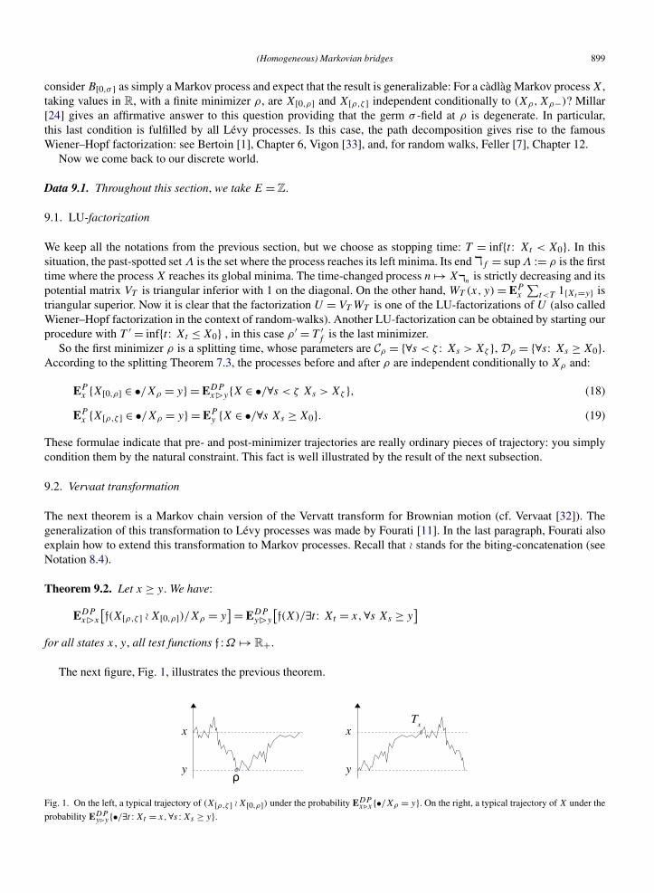
Theorem 9.2. Let x ≥ y. We have:
EDPx�x
[f(X[ρ,ζ ] � X[0,ρ])/Xρ = y
] = EDPy�y
[f(X)/∃t : Xt = x,∀s Xs ≥ y
]for all states x, y, all test functions f :Ω �→ R+.
The next figure, Fig. 1, illustrates the previous theorem.
Fig. 1. On the left, a typical trajectory of (X[ρ,ζ ] � X[0,ρ]) under the probability EDPx�x {•/Xρ = y}. On the right, a typical trajectory of X under the
probability EDPy�y {•/∃t : Xt = x,∀s : Xs ≥ y}.
900 V. Vigon
Proof. We consider S the splitting time with parameters
CS = {∀t Xt ≥ y,Xζ = x}, DS = {∀t < ζ Xt > y,X0 = x}.Clearly, under EP
y�y , the three events {∃t : Xt = x,∀s Xs ≥ y}, {S < ∞}, {XS = x} almost surely coincide. From thesplitting Theorem 7.3:
EDPy�y
[f(X)/∃t : Xt = x,∀t Xt ≥ y
] = EDPy�y
[f(X)/XS = x
]=
∫Ω2
f(ω � w)EDPy�x[X ∈ dω/∀t Xt ≥ y,Xζ = x]EDP
x�y[X ∈ dw/∀t < ζ Xt > y,X0 = x]
=∫
Ω2f(ω � w)EDP
y�x[X ∈ dω/∀t Xt ≥ y]EDPx�y[X ∈ dw/∀t < ζ Xt > y]
=∫
Ω2f(ω � w)EDP
y�x[X[ρ,ζ ] ∈ dω]EDPx�y[X[0,ρ] ∈ dw]
for the last step we used the bridge versions of (18) and (19). �
10. Extension of the universe
10.1. Adding an independent variable
Markov chains can also be defined on some probability space (Ω,E) which is not the canonical one. This makes itpossible to define some random elements independent of the Markov chain. By some classical coupling arguments(see Kallenberg [20], Chapter 5) the more general situation can described by the addition of only one independentrandom variable with a continuous law.
Let Ω = Ω × [0,1], the two canonical projections are denoted by X,ϑ . On Ω we define the probability EPx =
EPx ⊗ dv, where dv is the Lebesgue measure on [0,1]. We define similarly EDP
x�z. Thus, under EPx , X is a Markov
chain, ϑ is a U [0,1] variable, and X,ϑ are independent. ϑ represents all the extra randomness we need.
10.2. Randomized time
Random elements defined on Ω are called randomized variables. They can be written Z = Z(X,ϑ) (the “dot” justindicates that Z is an application that helps to understand Z). Let us consider a randomized time S = S(X,ϑ) :Ω �→N ∪ {��}. We have:
EPα
[f(X[0,S])1{XS=y}g(X[S,ζ ])
] = EPα
[∑t
�t (X)f(X[0,s])1{Xs=y}g(X[s,ζ ])],
where �t (X) = ∫ 10 1{S(X,v)=t} dv. We see that an estimation made at a randomized time can be interpreted by
a “weighted estimation,” but without leaving the canonical space.Reciprocally, every weighted estimation made with weight �t (X) such that
∑t �t (X) ≤ 1 can also be interpreted
by an estimation made at a randomized time defined by S(X, v) = inf{t : ∑s≤t �t (X) ≥ v}, inf ∅ = ��.
The weighted estimations, and particularly the ones made by “additive functionals,” are very important in thecontinuous time setting, see Blumenthal–Getoor [3], Chapter IV.
A randomized time S is a randomized splitting time such that there exist CS, DS , two measurable parts of Ω , suchthat:
on {t ≤ ζ } {S = t} = {(X[0,t], ϑ1) ∈ CS
} ∩ {(X[t,ζ ], ϑ2) ∈ DS
},
where ϑ1, ϑ2 are two independent uniform variables, which are functions of ϑ (thus independent of X). The random-ized stopping times are splitting times with second parameters D = Ω .
We can easily see that the splitting theorem is still valid in this context.
(Homogeneous) Markovian bridges 901
10.3. Randomized time-change
Let T = T (X,ϑ) be a randomized stopping time. Let (ϑn) be an i.i.d. sequence of U[0,1] constructed from ϑ (e.g.by extracting different sequences of decimal of the number ϑ ). We “iterate” T as follows:
�0 = 0,
�1 = �1(X,ϑ1) = T (X,ϑ1),
�2 = �2(X,ϑ1, ϑ2) = �1 + T (X[�1,ζ ], ϑ2),
�3 = �3(X,ϑ1, ϑ2, ϑ3) = �2 + T (X[�2,ζ ], ϑ3), etc.
We see that under EPx , the process n �→ X�n
is a Markov chain. We add the supplementary assumption that ∀x
EPx {T ≥ 1} > 0 which implies that a.s. the trajectories n �→ �n cannot be stopped at an integer k < ∞. In particular,
on {ζ < ∞}, the number �n is finite and we denote by �f the latest finite �n.
Proposition 10.1. Fix x, y, z ∈ E. We have:
EPx�z{X�f
= y}U(x, z) = EPx
[∑n
1{X�n=y}]
EPx
[∑t<T
1{Xt=y}].
Proof. By construction �(•, ϑ1, . . . , ϑn) are stopping times so that {�n = t} = {�(X[0,t], ϑ1, . . . , ϑn) = t}. Using thepast extraction and the independence between (ϑ1, . . . , ϑn) and ϑn+1 we get:
EPx�z{X�f
= y}=
∑n
EPx�z{X�n
= y,�n+1 = ∞}
=∑n
∑t
EPx�z
{�n(X[0,t], ϑ1 · · ·ϑn) = t,Xt = y, T (X[t,ζ ], ϑn+1) = ∞}
=∑n
∑t
EPx�z
{�n(X[0,t], ϑ1 · · ·ϑn) = t,Xt = y
}EP
y
{T (X,ϑ) = ∞}
.
The rest of the proof follows the same way as the end of the proof of Theorem 8.1. �
10.4. The comparison problem
Proposition 10.2. Let A :E × E �→ [0,1]. Let ϑ0, ϑ1, . . . an i.i.d. sequence of U[0,1], constructed from ϑ . Let SA =inf{t : ϑt > A(Xt ,Xt+1)} We have
EPx {X[0,SA] ∈ •} = EPA
x {X ∈ •},where PA(x, y) = P(x, y)A(x, y).
Proof. It is sufficient to check the equality for function of type f = 1{X0=x0,...,Xn=xn}:
EPx
[f(X[0,SA])
]= EP
x {X0 = x0, . . . ,Xn = xn,n ≤ SA}= EP
x
{X0 = x0, . . . ,Xn = xn,ϑ1 ≤ A(x0, x1), . . . , ϑn ≤ A(xn−1, xn)
}= P(x0, x1) · · ·P(xn−1, xn)A(x0, x1) · · ·A(xn−1, xn). �
902 V. Vigon
Remark 10.3. Of course the murder X �→ X[0,SA] is a generalization of the one introduced in Section 6. Such a murdercan be assimilated with murder by multiplicative functional, see Blumental and Getoor [3], Chapter III. The readercan also extend Theorem 6.1 in the extended universe.
Corollary 10.4. Let P,Q be two sub-stochastic matrices. P ≥ Q if and only if there exists a randomized time S suchthat EP
x {X[0,S] ∈ •} = EQx {X ∈ •}.
Proof. When P ≥ Q then we can find A: E × E ∈ [0,1] such that PA = Q, so the time S = SA works.Reciprocally, Q(x,y) = EQ
x {X1 = y} = EPx {X1 = y,1 ≤ S} ≤ P(x, y). �
Comments. Consider P,Q two sub-stochastic matrices. We see easily that:
P ≥ Q ⇒ U[P ] ≥ QU[P ].
We saw that the left-hand side inequality can be interpreted by a murder.Let us suppose now the right-hand side inequality: Rost [28] shows that this inequality implies the existence of a
randomized stopping time T such that Q(x,y) = EPx {XT = y}. Denoting by � the iteration of this stopping time, we
get the factorization U[P ] = U[Q]W where W(x,y) = EPx [∑t<T 1{Xt=y}]. Of course, this factorization can also be
directly deduced by putting W = U[P ] − QU[P ] ≥ 0 and then:
U[P ] = W + QU[P ] = W + QW + Q2U[P ] = · · · = U[Q]W.
To summarize, we have presented two ways to compare Markov chains: the first one is interpreted by a murder, thesecond one by a time-change. Of course, murder is a very particular case of time-change.
In a continuous-time setting, the interpretation of U[P ] = U[Q]W in terms of time-change as been done by Simon[30] for Lévy processes. The case of Markov processes has not been treated yet.
11. Extension to the Martin boundary
Data 11.1. Throughout this section, E is infinite and the undirected graph of P is irreducible and locally finite (i.e.there is a finite number of edges attached to each vertex).
11.1. A few reminders
Here we will recall definitions and basic results about the Martin Boundary. For a complete exposition, we send thereader to Dynkin [6], Hunt [16] or to the book of Woess [35]; our notations and hypotheses are the same as the onesin this book.
We choose any reference point o ∈ E. The Martin kernel is defined by:
K(x,y) = K[P,o](x, y) = U[P ](x, y)
U[P ](o, y)= EP
x {Ty < ∞}EP
o {Ty < ∞} .
A sequence (yn) is a Martin–Cauchy sequence if it leaves every finite subset of E, and if, for all x, the sequence n �→K(x,yn) converges. Two Martin–Cauchy sequences (yn) and (y′
n) are equivalent if for all x, we have limn K(x, yn) =limn K(x, y′
n). The Martin boundary does not depend on the reference point. Because K[DhP ](x, y) = h(o)h(x)
K[P ](x, y),the Martin boundary is the same for every matrix in DP . So we can denote the Martin boundary by M = M[DP ].
Elements of M will be generically denoted by ξ . Elements of E ∪ M will be generically denoted by η. On E ∪ M,we put the natural topology (e.g. yn converges to ξ ∈ M if and only if yn is an element of the equivalence class ξ )which makes E ∪ M a compact and metrizable space. The Martin kernel K is prolonged by continuity on M. It iseasy to verify that the excessive function x �→ K(x,η) (defined on E) is potential if η ∈ E and invariant if η ∈ M.
Remark 11.2. As a consequence, under our hypothesis, there always exists an invariant function (i.e. the Martinboundary has at least one point).
(Homogeneous) Markovian bridges 903
An excessive function h is said to be minimal if, for every excessive function h′ (non-identically zero), the inequal-ity h′ ≤ h implies that h′ and h are proportional. An excessive function h is said to be normalized if h(o) = 1. Theset of points ξ ∈ M such that K(•, ξ) is a minimal invariant function is denoted by Mmin. This set is Borelian in M.In some classical cases (e.g. Markov chain whose undirected graph is a tree, or random walks in Zd ) the sets M andMmin are equal. The set Mmin is more important for us, because it is the “target” where the canonical process finishesits life. This is the subject of the following theorem:
Theorem 11.3 (Convergence to the boundary). Under EPx , almost surely on {ζ = ∞}, the canonical process t �→ Xt
converges to a random variable X∞ taking values in Mmin. Moreover, we have:
EPx {Xζ = y, ζ < ∞} = K(x,y)EP
o {Xζ = y, ζ < ∞},EP
x {Xζ ∈ dξ, ζ = ∞} = K(x, ξ)EPo {Xζ ∈ dξ, ζ = ∞}.
Remark 11.4. The first equation of the theorem is an immediate consequence of the equality EPx {Xζ = y, ζ < ∞} =
U(x, y)P (y,†) established in Lemma 3.2. The second one can be seen as a prolongation of the first one. Both can besummarized as follows:
EPx {Xζ ∈ dη} = K(x,η)EP
o {Xζ ∈ dη} (20)
with the natural convention: Xζ = Xζ 1(ζ<∞) + X∞1(ζ=∞).The proof of the previous theorem, as well as the proof of the next one, can be readed in Woess [35], Chapter IV,
Section 24.
Theorem 11.5 (Representation with unicity). For every excessive function h, there exists a unique finite measure μ,supported by E ∪ Mmin such that:
h(x) =∫
E∪MK(x,η)μ(dη). (21)
This measure is given by
μ(dη) = EDhPo {Xζ ∈ dη}.
Corollary 11.6. The set of normalized minimal invariant functions is exactly {K(•, ξ): ξ ∈ Mmin}.
Remark 11.7. Of course, the equation (21) can be split into:
h(x) =∑a∈E
K(x, a)μ(a) +∫
MK(x, ξ)μ(dξ),
which gives the Riesz decomposition of h.
11.2. Prolongation of the bridge
Let us take ξ ∈ Mmin. Let us consider the normalized minimal invariant function K(•, ξ). Because of its invariantproperty, under EDK(•,ξ)P , the canonical process X has an infinite life. According to Theorem 11.3, this processconverges a.s. to X∞ ∈ M. Moreover we have obviously:
K(x, ξ) =∫
E∪MK(x,η)δξ (dη).
From the unicity of the measure in Theorem 11.5, we have:
EDK(•,ξ)Po {X∞ ∈ dη} = δξ (dη).
904 V. Vigon
We can summarize this as follows: Every normalized minimal invariant function K(•, ξ) leads the canonical processto a unique point ξ ∈ Mmin (in an infinite time); as well as, every normalized minimal potential function K(•, z) leadsthe canonical process to a unique state z ∈ E (in a finite time).
Here is the extension of the fundamental Lemma 3.4. The proof is similar and even simpler because now, theirreducible assumption, allows to replace D by D.
Lemma 11.8. Fix η ∈ E ∪ Mmin. Let P ′ be a matrix of DP . We have:
DK(•,η)P = DK ′(•,η)P′,
where K ′ = K[P ′,o] and K = K[P,o].
All these facts suggest to us the following definition:
Definition 11.9. For every η ∈ E ∪ Mmin we denote by P�η = DK(•,η)P and EDPx�η = E
P�ηx .
Because DK(•,z)P = DU(•,z)P , this definition is an extension of the one we have been using from the beginning.
11.3. Reconstruction of a Markov chain from its bridge
Theorem 11.10. We have the following identity between measure on Ω × E ∪ Mmin:
EPx {X ∈ dω,Xζ ∈ dη} = EDP
x�η{X ∈ dω}EPx {Xζ ∈ dη}.
Proof. It is sufficient to verify this equation on cylindrical functionals:
EPx {X0 = x0, . . . ,Xn = xn,Xζ ∈ dη}= EP
x
{X0 = x0, . . . ,Xn = xn, (Xζ ◦ X[n,ζ ]) ∈ dη
}= EP
x {X0 = x0, . . . ,Xn = xn}EPxn
{Xζ ∈ dη}= EP
x {X0 = x0, . . . ,Xn = xn}K(xn, η)EPo {Xζ ∈ dη}
= EPx {X0 = x0, . . . ,Xn = xn}K(xn, η)
K(x,η)EP
x {Xζ ∈ dη}
= EDPx�η{X0 = x0, . . . ,Xn = xn}EP
x {Xζ ∈ dη}. �
Remark 11.11. Let Q = DhP be a sub-stochastic matrix and α be a probability on E. The previous theorem gives:
EDhPα {X ∈ •} =
∑x∈E
∫η∈E∪M
α(x)EDPx�η{X ∈ •}EDhP
x {Xζ ∈ dη}.
This equation perfectly illustrates the following fact: A Markov chain can be parameterized by:
• An initial distribution α on E.• A mechanism of evolution given by the class of matrices DP .• A control given by a P -excessive function h.
11.4. Confinement
When η is such that EPx {Xζ = η} > 0 then, from Theorem 11.10, we have
EPx {X ∈ •/Xζ = η} = EDP
x�η{X ∈ •}
(Homogeneous) Markovian bridges 905
and thus the bridge can be seen as a final conditioning exactly as we treated it in Section 5. When EPx {Xζ = η} = 0
the right-hand side of the above equation has no sense, but, for convenience, we keep the notation�η−→ to designate
the “bridgification” i.e. the passage from EPx to EDP
x�η .We also use in this section the notations defined in Section 6.1. When ξ is an element of the Martin boundary, we
say that {x P� ξ} when there exists an infinite sequence x0 = x � x1 � x2, . . . such that (xi) belongs to the equivalentclass ξ .
Theorem 11.12. In all this theorem x ∈ E and ξ ∈ Mmin are such that {x PA� ξ}. We have:
EPx
X[0,SA]−−−−−→ �ξ−−−−−→ EDPA
x�ξ .
If EPx {XX ⊂ A} > 0 then we have:
EPx
/XX⊂A−−−−−→ �ξ−−−−−→ EDPA
x�ξ .
If EDPx�ξ {XX ⊂ A} > 0 then we have:
EPx
�ξ−−−−−→ /XX⊂A−−−−−→ EDPA
x�ξ .
This theorem is the direct extension of Theorem 6.1. The extension of the proof is left to the reader. Actually, wewrite this extension in order to illustrate a way to condition a Markov chain “to stay inside a set” when it is apparentlynot possible. Let us treat an example.
We consider an immortal Markov chain with state space Z. We suppose that its transition matrix P checks ourhypothesis, and that the Martin boundary of PZ+ is made by exactly one point that we denote by +∞. We supposemoreover that
∀x (⇔ ∃x) EPx {X∞ = +∞} = 0.
This last hypothesis implies that the event {X ⊂ Z+} := {∀t : Xt ≥ 0} is negligible under E0 (and under Ex for all x).Now, here is a classical question: how is it possible to condition the Markov chain E0 to stay positive? Answer:
this can be done by the two following operations:
EP0
�+∞−−−−−→ /X⊂Z+−−−−−→:= E+.
If intuitively (and not rigorously), you make the two operations commute, then E+ merits the name of “Markov chainconditioned to stay positive.”
Such conditioning often appears in the literature, especially when X is a random walk (see e.g. Bertoin [1], Chap-ter 7 or Biggins [2]). The recipes to make such conditioning are numerous (you can also condition by events withsmaller and smaller probabilities). Here we want to insist on the following fact: If your transition matrix (here P ),restricted to the set where you want to lock the Markov chain (here this set is Z+) has more than one point in itsMartin boundary, then such conditioning is ambiguous (you have to make an arbitrary choice for the final destinationof your process).
12. Un-normalized bridges
Data 12.1. Exceptionally in this section, P is any non-negative matrix.
When P is sub-stochastic, the existence of a recurrent point (i.e. EPx {∃t ≥ 1: Xt = x} = 1) implies non-transience
and forbids the construction of EDP•�•. In this section, we define σ -finite measures FPx�z which, in the transient case
are U[P ](x, z)EDPx�z but which can be defined for all non-negative P with finite spectral radius.
906 V. Vigon
12.1. Spectral radius
We recall some facts about spectral radii. These facts are quite well known, see Seneta [29], Chapter 6 or Woess [35],Chapter 2. Let us write:
Λ[P ] ={λ > 0:
1
λP is transient
},
it is clearly an interval of type ]ρ,∞[ or [ρ,∞[ for some ρ ∈ R+ ∪ {+∞}. This ρ, also noted ρ[P ], is called thespectral radius of P . Proposition 2.4 indicates that Λ[P ] = Λ[P]. Proposition 2.7 indicates that Λ[P ] = {λ > 0: ∃h >
0 which is 1λP -potential}. So we are tempted to compare Λ[P ] with:
Λ′[P ] := {λ ≥ 0: ∃h > 0: Ph ≤ λh}.
Lemma 12.2. We have Λ′[P ] = Λ[P ] or Λ′[P ] = Λ[P ] ∪ {ρ[P ]}.
Proof. Λ′ is clearly greater than Λ. So it is sufficient to show that the interior of Λ′ is included in the interior of Λ.Take λ ∈ Λ′ and h a 1
λP -excessive function. Take q ∈ ]0,1[. The matrix Q := q
λDhP is sub-stochastic and satisfies
U[Q]1E ≤ 11−q
1E . So λq
∈ Λ; and this is true for all q ∈ ]0,1[. �
Next we give an example of a sub-stochastic matrix P such that Λ[P ] �= Λ′[P ] and Λ′[P ] �= Λ′[P]. The matrix P
and its diagonalization are given by:
P =[
1 01/2 1/2
]=
[1 01 −1
][1 00 1/2
][1 01 −1
].
Here is its potential matrix:
U[P ] = (I − P)−1 =[
1 01 −1
][∞ 00 2
][1 01 −1
]=
[∞ 0∞ 2
].
So we get Λ[P ] = Λ[P] = ]1,∞[ while Λ′[P ] = [1,∞[ (because P 1E ≤ 1E). As it is impossible to solve P h ≤ h
with h > 0, we deduce that Λ′[P] = ]1,∞[.
The reader is also invited to check that the matrix P defined on E = N by P(n,m) = 1{m=n+1} has a spectral radiusρ = 0, while the matrix ∀m,n P (n,m) = 1 has a spectral radius ρ = +∞.
Of course, we are more accustomed to the irreducible case where the situation is easier to handle. The argument inWoess [35], p. 81, gives:
Proposition 12.3. Suppose that P is irreducible and ρ[P ] < ∞. Then we have Λ′[P ] = [ρ[P ],∞[.
Proof. Denote by Hλ the set of 1λP -excessive functions normalized by h(o) = 1 for some reference point o ∈ E. Take
λ such that Hλ �= ∅. By Fatou lemma Hλ is closed. By irreducibility, for all x there exists nx such that P nx (o, x) > 0.Thus, for h ∈ Hλ:
P nx (o, x)h(x) ≤ P nx h(o) ≤ λnx h(o).
Thus every function h of Hλ is bounded by the same function x �→ λnx f (o)P nx (o,x)
, so Hλ is compact. Finally, we see that⋂λ>ρ Hλ = Hρ �= ∅. �
To finish with these reminders about spectral radii, we explain the link with eigenvalues. Let us write Λ[P ] ={λ: ∃h > 0: Ph = λh}. Suppose P irreducible and E finite. Then the Perron–Frobenius theorem (see Seneta [29],p. 1) indicates that Λ[P ] = {ρ[P ]}. The absolute value of other eigenvalues are strictly less than ρ[P ] and ρ[P ] is the
(Homogeneous) Markovian bridges 907
only one to have an eigenvector everywhere positive. On the other hand, suppose P irreducible and E infinite, theMartin boundary (see Section 11) theory indicates that Λ[P ] = [ρ[P ],∞[. For a short direct proof of this fact, seeWoess [35], Lemma 7.6, p. 83).
12.2. Construction of un-normalized bridges
Data 12.4. From now on, and until the end of this section, we suppose that ρ[P ] < ∞.
Lemma 12.5. For i = 1,2, pick a real qi > 0 and a function hi > 0 such as Qi := qiDhiP is sub-stochastic. We have:
h1(x)
h1(z)EQ1
x
[∑t
q−t1 f(X[0,t])1{Xt=z}
]= h2(x)
h2(z)EQ2
x
[∑t
q−t2 f(X[0,t])1{Xt=z}
].
Proof. It is sufficient to establish this formula, replacing f by 1{X0=x0,...,xn=xn}. Doing this and computing, we see thatall hi, qi disappear. �
Definition 12.6. Pick real q > 0 and a function h > 0 such that qDhP is sub-stochastic. We define the kernel
FPx�z
[f(X)
] = h(x)
h(y)EqDhP
x
[∑t
q−t f(X[0,t])1{Xt=z}]
which is called the un-normalized Markov-bridge-kernel. From the previous lemma, this definition does not dependon the choice of (q,h).
We see immediately that FPx�z is supported by {ζ < ∞} and that its total mass is U[P ](x, z) which can be infinite.
We give now some direct consequences of Definition 12.6 and Proposition 12.5:
• When P is sub-stochastic:
FPx�z = EP
x
[∑t
1{X[0,t]∈•}1{Xt=z}]. (22)
• When P is transient, we have:
FPx�z = EDP
x�z{X ∈ •}U(x, z). (23)
• For q ∈ R, we have:
FqPx�z = FP
x�z
[1{X∈•}qζ
]. (24)
Remark 12.7.
• From (24), taking q sufficiently small, we see that for any P , ∀s FPx�z{ζ = s} < ∞.
• For P sub-stochastic, from (22) we can compute FPx�z{X ∈ •/ζ = s} = EP
x {X ∈ •/Xs = z} which is the sameformula that the one with the normalized bridge (conditionning make the normalization). We can also rewrite thisas: FP
x�z{X ∈ •, ζ = s} = EPx {X ∈ •/Xs = z}P s(x, z) and compare this with the formula given by Fourati [11],
Proposition 5.1.
12.3. Past-future extraction and time reversal
Theorem 12.8. We have:
FPx�y
[f(X)
]FP
y�z
[g(X)
] = FPx�z
[∑t
f(X[0,t])1{Xt=y}g(X[t,ζ ])]
(25)
for all states x, y, z ∈ E, all test functions f,g :Ω �→ R+.
908 V. Vigon
Proof. First suppose that P is transient. Formula (25) is simply the combination of (23) and of the past–future extrac-tion (Theorem 3.5) wrote as follows:
EDPx�y
[f(X)
]U(x, y)EDP
y�z
[g(X)
]U(y, z) = EDP
x�z
[∑t
f(X[0,t])1{Xt=y}g(X[t,ζ ])]U(x, z).
Now suppose P has just a finite spectral radius. Take q > 0 such that qP is transient. Applying (25) to qP and using(24) we get:
FPx�y
[f(X)qζ
]Fy�z
[g(X)qζ
] = FPx�z
[∑t
f(X[0,t])qt1{Xt=y}g(X[t,ζ ])qζ−t
]
= FPx�z
[∑t
(fqζ
) ◦ X[0,t]1{Xt=y}(gqζ
) ◦ X[t,ζ ]].
The result follows by substituating f := fq−ζ and g := gq−ζ . �
Proposition 12.9. When x � z we have FPx�z{X ∈ •} = FP
z�x{X ←[0,ζ ]∈ •}.
Proof. Suppose P transient. From Theorem 4.3: EDPx�z = EDP
z�x {X ←[0,ζ ]∈ •}. Multiplying at the left by U[P ](x, z) and
at the right by the same quantity written U[P](z, x), we obtain Proposition 12.9. The non-transient case follows byworking with P := qP , as in the previous proof. �
12.4. Application
Let us explain briefly how the last proposition can be used to prove the following classical result:
Proposition 12.10. Suppose P sub-stochastic. Let μ > 0 a P -excessive measure. Denote by P = DμP . We have:
μ(a)EPa
[ ∑t<T ∗
A
1{Xt=y}]
1{a∈A} = μ(y)EPy {XTA
= a},
where TA = inf{t ≥ 0: Xt ∈ A} and T ∗A = inf{t ≥ 1: Xt ∈ A}.
Remark 12.11. Suppose that EPy {Tx < ∞} = 1. The above equation, applied with A = {x} becomes
μ(x)EPx [∑t<T ∗
x1{Xn=y}] = μ(y), which is a very famous formula of the recurrent theory of Markov chains.
Proof of Proposition 12.10. Pick a ∈ A,y ∈ E. Having a look at Fig. 2 we see that:
1{X0=a}1{t<T ∗A}1{Xt=y} = 1{X0=a}1{TA=t} ◦ X←[0,t]
1{Xt=y}
= 1{X0=a}1{TA=ζ } ◦ X ←[0,ζ ]◦ X[0,t]1{Xt=y}.
Summing over all t , integrating, and using (22) we get:
EPa
[ ∑t<T ∗
A
1{Xt=y}]
= FPa�y[1{TA=ζ } ◦ X ←[0,ζ ]
].
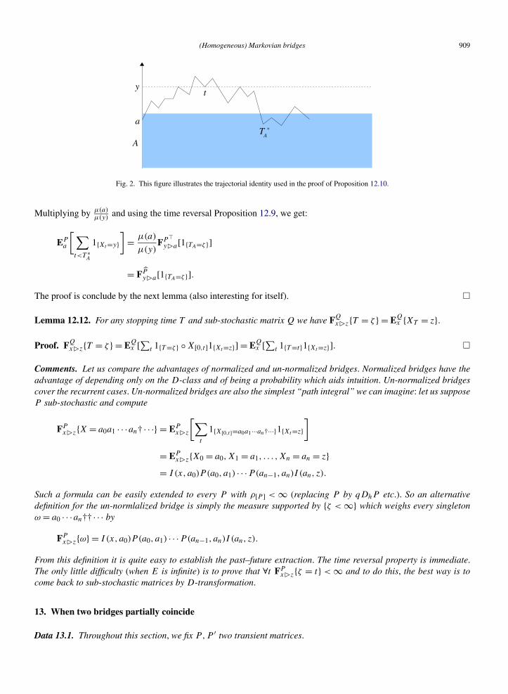
(Homogeneous) Markovian bridges 909
Fig. 2. This figure illustrates the trajectorial identity used in the proof of Proposition 12.10.
Multiplying by μ(a)μ(y)
and using the time reversal Proposition 12.9, we get:
EPa
[ ∑t<T ∗
A
1{Xt=y}]
= μ(a)
μ(y)FP
y�a[1{TA=ζ }]
= FPy�a[1{TA=ζ }].
The proof is conclude by the next lemma (also interesting for itself). �
Lemma 12.12. For any stopping time T and sub-stochastic matrix Q we have FQx�z{T = ζ } = EQ
x {XT = z}.
Proof. FQx�z{T = ζ } = EQ
x [∑t 1{T =ζ } ◦ X[0,t]1{Xt=z}] = EQx [∑t 1{T =t}1{Xt=z}]. �
Comments. Let us compare the advantages of normalized and un-normalized bridges. Normalized bridges have theadvantage of depending only on the D-class and of being a probability which aids intuition. Un-normalized bridgescover the recurrent cases. Un-normalized bridges are also the simplest “path integral” we can imagine: let us supposeP sub-stochastic and compute
FPx�z{X = a0a1 · · ·an† · · ·} = EP
x�z
[∑t
1{X[0,t]=a0a1···an†···}1{Xt=z}]
= EPx�z{X0 = a0,X1 = a1, . . . ,Xn = an = z}
= I (x, a0)P (a0, a1) · · ·P(an−1, an)I (an, z).
Such a formula can be easily extended to every P with ρ[P ] < ∞ (replacing P by qDhP etc.). So an alternativedefinition for the un-normlalized bridge is simply the measure supported by {ζ < ∞} which weighs every singletonω = a0 · · ·an†† · · · by
FPx�z{ω} = I (x, a0)P (a0, a1) · · ·P(an−1, an)I (an, z).
From this definition it is quite easy to establish the past–future extraction. The time reversal property is immediate.The only little difficulty (when E is infinite) is to prove that ∀t FP
x�z{ζ = t} < ∞ and to do this, the best way is tocome back to sub-stochastic matrices by D-transformation.
13. When two bridges partially coincide
Data 13.1. Throughout this section, we fix P,P ′ two transient matrices.
910 V. Vigon
Notations. For K ⊂ E we write PK(x, y) for P(x, y)1{x∈K}1{y∈K} and DPK for D(PK). Thus DPK = DP ′K if and
only if there exists h > 0 such that ∀x, y ∈ K P(x,y) = h(y)h(x)
P ′(x, y). In this situation we say that DP,DP ′ coincideon K .
For K ⊂ E × E we write PK(x, y) for P(x, y)1{xy∈K} etc.
13.1. Closed set
A set K ⊂ E is said P -closed when K = {K P� • P� K}. This means that every chain beginning and ending in K has
all its elements in K . It is easy to see that any set of type {A P� • P� C} is P -closed. In particular, P -absorbing andP -absorbing sets are P -closed.
The main interest of a P -closed set K is that:
∀x, z ∈ K EDPx�z{X ∈ •} = EDP
x�z{X ∈ •/X ⊂ K} = EDPKx�z {X ∈ •} (26)
(the last equality comes from Theorem 6.1). As a consquence, when K is P -closed and P ′-closed then:
DPK = DP ′K ⇒ ∀x, z ∈ K EDP
x�z = EDP ′x�z.
The purpose of the rest of this section is to establish some converse of this implication.
13.2. Simple coincidence
Proposition 13.2. Fix x, z ∈ E. The following points are equivalents:
1. EDPx�z = EDP ′
x�z.
2. We have {x P� • P� z} = {x P ′� • P ′
� z} and DP,DP ′ coincide on this set.
Proof. 1 ⇒ 2. We have:
{b :xP� b
P� z} = {b: EDP
x�z{∃t : Xt = b} > 0}
= {b: EDP ′
x�z{∃t : Xt = b} > 0} = {b :x
P ′� b
P ′� z}
this set will be simply denoted by {x � • � z}. If this set is reduced to {x, z}, then xP�� z and x
P ′�� z and in this case
the second point is obviously true. Let us now assume that xP� z. We fix a, b ∈ {x � • � z}. We have
P�z(a, b) = EDPx�z{XTa+1 = b/Ta < ∞}
= EDP ′x�z{XTa+1 = b/Ta < ∞} = P ′
�z(a, b),
this equality means: U(b,z)U(a,z)
P (a, b) = U ′(b,z)U ′(a,z)
P ′(a, b), so we have
P ′(a, b) = h(b)
h(a)P (a, b) with h(•) = U(•, z)
U ′(•, z)
which said that DP and DP ′ coincide on {x � • � z}.2 ⇒ 1. This comes from the fact that {x P� • P� z} = {x P ′
� • P ′� z} is a P and P ′ closed set (see previous subsec-
tion). �
The previous proposition cannot be generalized replacing {x P� • P� z} by any closed set. To understood the prob-lem, we need to make some specific graph theory.
(Homogeneous) Markovian bridges 911
13.3. Directed-spanning-tree
An directed tree is a directed graph (B,Υ→) such that its undirected version has no cycle, and such that there exists
one element o called “center” such that for every b ∈ B we have oΥ� b or b
Υ� o. The degenerated graph with onevertex, zero edge is a directed tree.
We say that a graph (B,→) admits a directed-spanning-trees when each of its connected component C admitsa sub-graph which is a directed-tree linking every vertex of C.
If there exists x ∈ B such that B = {x � •} then (B,→) admits a directed-spanning-tree (to see this, explore B
from x, replacing cycles by branchings). By symmetry: if there exists z ∈ B such that B = {• � z} then (B,→) admitsa directed-spanning-tree. In particular, if P is irreducible then its directed graph admits a directed-spanning-tree.
Lemma 13.3. Suppose that (E,P→) or (E,
P ′→) admits a directed-spanning-tree. We have DP = DP ′ if and only if,
for all x, z ∈ E, we have {x P� • P� z} = {x P ′� • P ′
� z} and DP,DP ′ coincide on this set.
Proof. Direct sense is obvious. Let us prove the converse. The equality ∀x, z {x P� • P� z} = {x P ′� • P ′
� z} implies
(E,P→) = (E,
P ′→). This graph is now denoted by (E,→). Moreover, without loss of generality, we can assume thatthis graph has only one connected component (if not, we solve the problem on each component separately).
We denote by γ (a, b) = P(a,b)P ′(a,b)
with 00 = 0. The hypothesis indicates that:
∀x, z ∈ E ∃hx,z > 0: ∀a, b ∈ {x � • � z}: γ (a, b) = hxz(b)
hxz(a)1{a�b}
(our aim is to find a function h not depending on x, z). This implies in particular that:
x � y � z ⇒ γ (x, z) = γ (x, y)γ (y, z). (27)
Let us consider a directed spanning tree (E,Υ→) with central point o. Let x ∈ E and let x = a0, a1, a2, . . . , an−1, an = z
be the unique chain going from o to x or from x to o in the tree. We define a function h > 0 as follows:
h(o) = 1,
when oΥ� x, h(x) = γ (o, a1)γ (a1, a2) · · ·γ (an−1, x),
when x� o, h(x) = 1
γ (o, a1)
1
γ (a1, a2)· · · 1
γ (an−1, x).
Therefore, by construction:
aΥ� o ⇒ γ (a, o) = h(o)
h(a)and o
Υ� a ⇒ γ (o, a) = h(a)
h(o). (28)
Let us verify that:
∀a, b ∈ E γ (a, b) = h(b)
h(a)1{a�b}. (29)
If a �� b then this equation become 0 = 0. We suppose now that a � b.
• If aΥ� o and b
Υ� o then we have a � b � o and (27) implies γ (a, b)γ (b, o) = γ (a, o). Using (28) we get (29).
• If aΥ� o
Υ� b then (28) gives directly (29).
• If oΥ� a and o
Υ� b then we have o � a � b and (27) implies γ (o, b) = γ (a, o)γ (a, b). Using (28) we get (29).
• If oΥ� a and b
Υ� o then we have a � b � o and (27) implies γ (a, o) = γ (a, b)γ (b, o). Using (28) we get (29). �
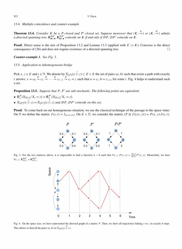
912 V. Vigon
13.4. Multiple coincidence and counter-example
Theorem 13.4. Consider K be a P -closed and P ′-closed set. Suppose moreover that (K,P→) or (K,
P ′→) admitsa directed-spanning-tree. EDP•�•,EDP ′
•�• coincide on K if and only if DP,DP ′ coincide on K .
Proof. Direct sense is the mix of Proposition 13.2 and Lemma 13.3 (applied with E := K). Converse is the directconsequence of (26) and does not require existence of a directed spanning tree. �
Counter-example 1. See Fig. 3.
13.5. Application to inhomogeneous bridge
Pick x, z ∈ E and t ∈ N. We denote by K[P ](xt� z) ⊂ E ×E the set of pairs (a, b) such that exists a path with exactly
t arrows: x = c0P→ c1
P→ ·· · P→ ct−1P→ ct = z such that a = ci, b = ci+1 for some i. Fig. 4 helps to understand such
a set.
Proposition 13.5. Suppose that P,P ′ are sub-stochastic. The following points are equivalent:
• EPx {X[0,t]/Xt = z} = EP ′
x {X[0,t]/Xt = z}.• K[P ](x
t� z) = K[P ′](x
t� z) and DP,DP ′ coincide on this set.
Proof. To come back on our homogeneous situation, we use the classical technique of the passage to the space–time:On N we define the matrix J (s, t) = 1{t=s+1}. On E × N, we consider the matrix (P ⊗ J )(xs, yt) = P(x, y)J (s, t).
Fig. 3. For the two matrices above, it is impossible to find a function h > 0 such that ∀x, y P (x, y) = h(y)h(x)
P ′(x, y). Meanwhile, we have
∀x, z: EDPx�z = EDP ′
x�z .
Fig. 4. On the space axis, we have represented the directed graph of a matrix P . Then, we draw all trajectories linking x to z in exactly 6 steps.
This allows to find all the pairs (a, b) in K[P ](x6� z).
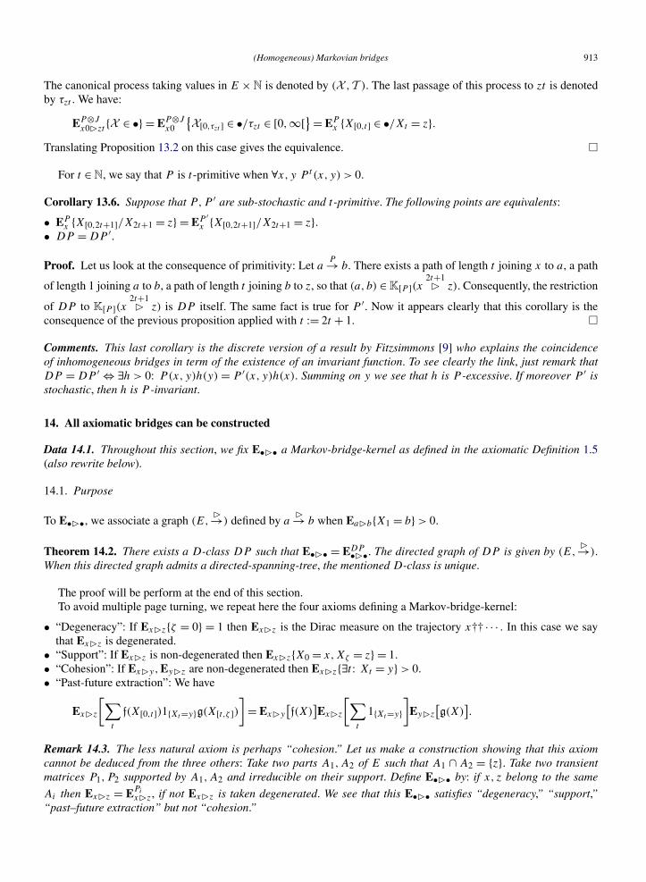
(Homogeneous) Markovian bridges 913
The canonical process taking values in E × N is denoted by (X , T ). The last passage of this process to zt is denotedby τzt . We have:
EP⊗Jx0�zt {X ∈ •} = EP⊗J
x0
{X[0,τzt ] ∈ •/τzt ∈ [0,∞[} = EP
x {X[0,t] ∈ •/Xt = z}.Translating Proposition 13.2 on this case gives the equivalence. �
For t ∈ N, we say that P is t -primitive when ∀x, y P t (x, y) > 0.
Corollary 13.6. Suppose that P,P ′ are sub-stochastic and t -primitive. The following points are equivalents:
• EPx {X[0,2t+1]/X2t+1 = z} = EP ′
x {X[0,2t+1]/X2t+1 = z}.• DP = DP ′.
Proof. Let us look at the consequence of primitivity: Let aP→ b. There exists a path of length t joining x to a, a path
of length 1 joining a to b, a path of length t joining b to z, so that (a, b) ∈ K[P ](x2t+1� z). Consequently, the restriction
of DP to K[P ](x2t+1� z) is DP itself. The same fact is true for P ′. Now it appears clearly that this corollary is the
consequence of the previous proposition applied with t := 2t + 1. �
Comments. This last corollary is the discrete version of a result by Fitzsimmons [9] who explains the coincidenceof inhomogeneous bridges in term of the existence of an invariant function. To see clearly the link, just remark thatDP = DP ′ ⇔ ∃h > 0: P(x, y)h(y) = P ′(x, y)h(x). Summing on y we see that h is P -excessive. If moreover P ′ isstochastic, then h is P -invariant.
14. All axiomatic bridges can be constructed
Data 14.1. Throughout this section, we fix E•�• a Markov-bridge-kernel as defined in the axiomatic Definition 1.5(also rewrite below).
14.1. Purpose
To E•�•, we associate a graph (E,�→) defined by a
�→ b when Ea�b{X1 = b} > 0.
Theorem 14.2. There exists a D-class DP such that E•�• = EDP•�•. The directed graph of DP is given by (E,�→).
When this directed graph admits a directed-spanning-tree, the mentioned D-class is unique.
The proof will be perform at the end of this section.To avoid multiple page turning, we repeat here the four axioms defining a Markov-bridge-kernel:
• “Degeneracy”: If Ex�z{ζ = 0} = 1 then Ex�z is the Dirac measure on the trajectory x†† · · · . In this case we saythat Ex�z is degenerated.
• “Support”: If Ex�z is non-degenerated then Ex�z{X0 = x,Xζ = z} = 1.• “Cohesion”: If Ex�y,Ey�z are non-degenerated then Ex�z{∃t : Xt = y} > 0.• “Past-future extraction”: We have
Ex�z
[∑t
f(X[0,t])1{Xt=y}g(X[t,ζ ])]
= Ex�y
[f(X)
]Ex�z
[∑t
1{Xt=y}]
Ey�z
[g(X)
].
Remark 14.3. The less natural axiom is perhaps “cohesion.” Let us make a construction showing that this axiomcannot be deduced from the three others: Take two parts A1,A2 of E such that A1 ∩ A2 = {z}. Take two transientmatrices P1,P2 supported by A1,A2 and irreducible on their support. Define E•�• by: if x, z belong to the same
Ai then Ex�z = EPix�z, if not Ex�z is taken degenerated. We see that this E•�• satisfies “degeneracy,” “support,”
“past–future extraction” but not “cohesion.”
914 V. Vigon
14.2. Lemmas
Corollary 1.9 indicates that E•�z is a mortal Markov-chain-kernel. We denote by P�z its transition matrix.
Lemma 14.4. We have
Ex�z{∃t : Xt = y} > 0 ⇒ Ex�z
{X[0,τy ] ∈ •/τy ∈ [0,∞[} = Ex�y. (30)
Proof. We already proved this for constructed bridges EP•�• (Theorem 5.1, first item). This proof only required thepast–future extraction which is also true for our axiomatic bridge E•�•. �
For a graph (E,→) we write x ∗� y to indicate that there exists a chain x → ·· · → y and that this chain isnot degenerated (has at least one arrow). For example, for the directed graph of a sub-stochastic matrix Q, we have
xQ∗� y ⇔ EQ
x {∃t ≥ 1: Xt = y} > 0, while xQ� y ⇔ EQ
x {∃t ≥ 0: Xt = y} > 0.
Lemma 14.5. We have x�∗� y if and only if Ex�y is not degenerated.
Proof. Suppose x�∗� y. Suppose that the linking chain has n ≥ 1 arrows: x
�→ a1�→ ·· · �→ an = y. This force Ex�a1
and Ea1�a2 to be non-degenerated. From the “cohesion” axiom, Ex�a2 is non-degenerated. By induction we deducethat Ex�y is non-degenerated.
Conversely, suppose Ex�y non-degenerated i.e. Ex�y{ζ ≥ 1} > 0. From “support axiom” Ex�y{∃t ≥ 1: Xt =y} > 0 and so there exists a chain with n ≥ 1 arrows x
P�y→ a1P�y→ ·· · P�y→ an = y. From (30):
Ex�a1{X1 = a1} = Ex�y
{(X[0,τa1 ])1 = a1 ∈ •/τa1 ∈ [0,∞[}
= Ex�y{X1 = a1} = P�y(x, a1) > 0.
By induction we deduce that Eai�ai+1{X1 = ai+1} > 0 for all i. �
Lemma 14.6. Fix z ∈ E. For all a, b ∈ {• �� z} we have Ea�b = EP�z
a�b.
Proof. If b = z then the statement is a tautology, so we suppose b �= z.
Case 1: a�∗� b. So, from Lemma 14.5, Ea�b is not degenerated. Because b
�� z and b �= z we also have a�∗� b
and so Eb�z is non-degenerated. From “cohesion” axiom Ea�z{∃t : Xt = b} > 0 and from (30) we deduce:
Ea�b = Ea�z
{X[0,τb] ∈ •/τb ∈ [0,∞[} = EP�z
a�b.
Case 2: a�∗�� b. From Lemma 14.5 Ea�b is degenerated. If EP�y
a�b would not be degenerated, (30) would bringa contradiction. �
14.3. Proof of Theorem 14.2
Existence: We add to our state space a point
†
which will play the role of a birth point. So our new state space is now{ †} ∪E ∪{†}. Let α > 0 be a probability on E. We define (Ex�z)x,z∈{ †}∪E by: ∀x, z ∈ E Ex�z = Ex�z, ∀x ∈ E Ex� †
is degenerated, ∀z ∈ E E †�z is the law of a trajectory going from
†
to a in one step with probability α(a) and thengoing from a to z following the law Ea�z. It is straightforward that this new kernel is still a Markov-bridge-kernel.
We consider its reversed version E•�• (see Remark 1.6). The associated graph is denoted by ({ †} ∪ E,
�→). By
construction we have ∀a ∈ E a�� †
. Let Q be the transition matrix of E•� †; this matrix is defined on { †} ∪ E.
Lemma 14.6 shows that E•�• = EDQ
•�• and from Theorem 4.3 we get that E•�• = EDQ•�• . Taking P as the restriction
of Q to E, E being Q-closed, we get E•�• = EDP•�•.
(Homogeneous) Markovian bridges 915
Graph: Let P be the matrix constructed previously. We have:
a�→ b ⇔ Ea�b{X1 = b} > 0
⇔ EDPa�b{X1 = b} > 0
⇔ U[P ](b, b)
U[P ](a, b)P (a, b) > 0 with
0
0= 0
⇔ P(a, b) > 0.
We deduce that the directed graph of P is (E,�→).
Unicity: Suppose E•�• = EDP•�• = EDP ′•�•. From the previous point, directed graphs of P,P ′ are (E,
�→) whose, byhypothesis, admits a directed spanning tree. Theorem 13.4, applied with K = E, gives DP = DP ′.
Acknowledgments
Thank you to Andrew Eastman who kindly change my frenglish into english. Thank you to the referee who, by hisnumerous suggestions, has really contributed to improve this article.
References
[1] J. Bertoin. Lévy Processes. Cambridge Tracts in Mathematics 121. Cambridge Univ. Press, Cambridge, 1998. MR1406564[2] J. D. Biggins. Random walk conditioned to stay positive. J. London Math. Soc. (2) 67 (2003) 259–272. MR1942425[3] R. M. Blumenthal and R. K. Getoor. Markov Processes and Potential Theory. Pure and Applied Mathematics 29. Academic Press, New
York–London, 1968. MR0264757[4] C. Dellacherie and P.-A. Meyer. Probabilités et potentiel. Chapitres IX à XI: Théorie discrète du potentiel. Publications de l’Institut de
Mathématique de l’Université de Strasbourg XVIII. Actualités Scientifiques et Industrielles 1410. Hermann, Paris, 1983. MR0727641[5] J. L. Doob. Conditional Brownian motion and the boundary limits of harmonic functions. Bull. Soc. Math. France 85 (1957) 431–458.
MR0109961[6] E. B. Dynkin. Boundary theory of Markov processes (the discrete case). Russian Math. Surveys 24 (1969) 1–42. MR0245096[7] W. Feller. An Introduction to Probability Theory and Its Applications, Vol. II, 2nd edition. Wiley, 1966. MR0210154[8] P. J. Fitzsimmons. On the excursions of Markov processes in classical duality. Probab. Theory Related Fields 75 (1987) 159–178. MR0885460[9] P. Fitzsimmons. Markov processes with identical bridges. Electron. J. Probab. 3 (1998). MR1641066
[10] P. Fitzsimmons, J. Pitman and M. Yor. Markovian bridges: Construction, Palm interpretation, and splicing. In Seminar on Stochastic Processes101–134. Progress in Probability 33. Birkhäuser Boston, Boston, 1992. MR1278079
[11] S. Fourati. Vervaat et Lévy. Ann. Inst. H. Poincaré Probab. Statist. 41 (2005) 461–478. MR2139029[12] R. K. Getoor and M. J. Sharpe. The Markov property at co-optional times. Z. Wahrsch. Verw. Gebiete 48 (1979) 201–211. MR0534845[13] R. K. Getoor and M. J. Sharpe. Excursions of dual processes. Adv. Math. 45 (1982) 259–309. MR0673804[14] J. Hoffmann-Jørgensen. Markov sets. Math. Scand. 24 (1969) 145–166. MR0256460[15] G. A. Hunt. Markoff processes and potentials. Illinois J. Math. 2 (1958) 151–213. MR0107097[16] G. A. Hunt. Markoff chains and Martin boundaries. Illinois J. Math. 4 (1960) 316–340. MR0123364[17] K. Itô. Poisson point processes attached to Markov processes. In Proceedings of the Sixth Berkeley Symposium on Mathematical Statistics
and Probability, Vol. III: Probability Theory 225–239. Univ. California Press, Berkeley, 1972. MR0402949[18] M. Jacobsen. Splitting times for Markov processes and a generalised Markov property for diffusions. Z. Wahrsch. Verw. Gebiete 30 (1974)
27–43. MR0375477[19] M. Jacobsen and J. M. Pitman. Birth, death and conditioning of Markov chains. Ann. Probab. 5 (1977) 430–450. MR0445613[20] O. Kallenberg. Foundations of Modern Probability, 2nd edition. Probability and Its Applications (New York). Springer, New York, 2002.
MR1876169[21] A. N. Kolmogorov. Zur Theorie der Markoffschen Ketten. Math. Ann. 112 (1936) 155–160. MR1513044[22] B. Maisonneuve. Sytèmes régénératifs. Astérique 15. Société mathématique de France, 1974. MR0350879[23] P. A. Meyer, R. T. Smythe and J. B. Walsh. Birth and death of Markov processes. In Proceedings of the Sixth Berkeley Symposium on
Mathematical Statistics and Probability, Vol. III: Probability Theory 295–305. Univ. California Press, Berkeley, 1972. MR0405600[24] P. W. Millar. Zero–one laws and the minimum of a Markov process. Trans. Amer. Math. Soc. 226 (1977) 365–391. MR0433606[25] M. Nagasawa. Time reversions of Markov processes. Nagoya Math. J. 24 (1964) 177–204. MR0169290[26] J. Pitman and M. Yor. Itô’s excursion theory and its applications. Japan J. Math. 2 (2007) 83–96. MR2295611[27] A. O. Pittenger and C. T. Shih. Coterminal families and the strong Markov property. Trans. Amer. Math. Soc. 182 (1973) 1–42. MR0336827[28] H. Rost. Markoff–Ketten bei sich füllenden Löchern im Zustandsraum. Ann. Inst. Fourier (Grenoble) 21 (1971) 253–270. MR0299755

916 V. Vigon
[29] E. Seneta. Non-Negative Matrices. An Introduction to Theory and Applications. Allen & Unwin, London, 1973. MR0389944[30] T. Simon. Subordination in the wide sense for Lévy processes. Probab. Theory Related Fields 115 (1999) 445–477. MR1728917[31] H. Thorisson. Coupling, Stationarity, and Regeneration. Probability and Its Applications (New York). Springer, New York, 2000. MR1741181[32] W. Vervaat. A relation between Brownian bridge and Brownian excursion. Ann. Probab. 7 (1979) 141–149. MR0515820[33] V. Vigon. Simplifiez vos Lévy en titillant la factorisation de Wiener–Hopf. Editions Universitaires Europeennes, also disposable on HAL and
on my web page, 2002.[34] D. Williams. Decomposing the Brownian path. Bull. Amer. Math. Soc. 76 (1970) 871–873. MR0258130[35] W. Woess. Random Walks on Infinite Graphs and Groups. Cambridge Tracts in Mathematics 138. Cambridge Univ. Press, Cambridge, 2000.
MR1743100


![Utilisation de modèles markoviens poursahbi/publication-238.pdf · 2017. 9. 21. · recalage d'images est une problématique classique en vision arti cielle [25], et se fait généralement](https://img.pdfslide.net/doc/110x75/60857267c309e8608b100c79/utilisation-de-modles-markoviens-pour-sahbipublication-238pdf-2017-9-21.jpg)