Embed Size (px)
Citation preview
Homogenization and asymptotics for small transaction costs:the multidimensional case
Dylan Possamaï ∗ H. Mete Soner† Nizar Touzi‡
Numerical results by: Loïc Richier and Bertrand Rondepierre§
January 20, 2013
Abstract
In the context of the multi-dimensional infinite horizon optimal consumption in-vestment problem with small proportional transaction costs, we prove an asymptoticexpansion. Similar to the one-dimensional derivation in our accompanying paper [42],the first order term is expressed in terms of a singular ergodic control problem. Ourarguments are based on the theory of viscosity solutions and the techniques of ho-mogenization which leads to a system of corrector equations. In contrast with theone-dimensional case, no explicit solution of the first corrector equation is availableand we also prove the existence of a corrector and its properties. Finally, we providesome numerical results which illustrate the structure of the first order optimal controls.
Key words: transaction costs, homogenization, viscosity solutions, asymptotic expan-sions.
AMS 2000 subject classifications: 91B28, 35K55, 60H30.
JEL classifications: D40, G11, G12, 60H30.
∗CEREMADE, Université Paris Dauphine, [email protected].†ETH (Swiss Federal Institute of Technology), Zurich, and Swiss Finance Institute, [email protected].
Research partly supported by the European Research Council under the grant 228053-FiRM, the SwissFinance Institute and by the ETH Foundation.
‡CMAP, Ecole Polytechnique Paris, [email protected]. Research supported by the Chair Fi-nancial Risks of the Risk Foundation sponsored by Société Générale, and the Chair Finance and SustainableDevelopment sponsored by EDF and Calyon.
§Ecole Polytechnique Paris, [email protected], [email protected].
1
1 Introduction
We continue our asymptotic analysis of problems with small transaction costs using theapproach developed in [42] for problems with only one stock. In this paper, we consider thecase of multi stocks with proportional transaction costs. The problem of investment andconsumption in such a market was first studied by Magill & Constantinides [29] and laterby Constantinides [11]. There is a large literature including the classical papers of Davis &Norman [13], Shreve & Soner [40] and Dumas & Luciano [14]. We refer to our earlier paper[42] and to the recent book of Kabanov & Safarian [26] for other references and for moreinformation.
This problem is an important example of a singular stochastic control problem. It is wellknown that the related partial differential equation contains a gradient constraint. As suchit is an interesting free boundary problem. The main focus of this paper is on the analysis ofthe small transaction costs asymptotics. It is clear that in the limit of zero transaction costs,we recover the classical problem of Merton [31] and the main interest is on the derivationof the corrections of this obvious limit.
The asymptotic problem is a challenging problem which attracted considerable attention inthe existing literature. The first rigorous proof in this direction was obtained in the appendixof [40]. Later several rigorous results [5, 21, 25, 35] and formal asymptotic results [1, 22, 44]have been obtained. The rigorous results have been restricted to one space dimensions withthe exception of the recent manuscript by Bichuch and Shreve [6].
In this paper, we use the techniques developed in [42]. As in that paper, the main techniqueis the viscosity approach of Evans to homogenization [15, 16]. This powerful method com-bined with the relaxed limits of Barles & Perthame [2] provides the necessary tools. As wellknown, this approach has the advantage of using only a simple L∞ bound. In addition to[2, 15, 16], the rigorous proof utilizes several other techniques from the theory of viscositysolutions developed in the papers [2, 17, 19, 27, 34, 37, 41] for asymptotic analysis.
For the classical problem of homogenization, we refer to the reader to the classical papersof Papanicolau & Varadhan [33] and of Souganidis [43]. However, we emphasize that theproblem studied here does not even look like a typical homogenization problem of the ex-isting literature. Indeed, the dynamic programming equation, which is the starting point ofour asymptotic analysis, does not include oscillatory variables of the form x/ε or in generala fast varying ergodic quantity. The fast variable appears after a change of variables thatincludes the difference with the optimal strategy at the effective level problem. Hence, thefast variable actually depends upon the behavior of the limit problem, which is a novel view-point for homogenization where usually the fast variables are built into the equation fromthe beginning and one does not have to construct them from limits. This ergodic variable, ingeneral, does not have to be periodic. In recent studies, deep techniques combining ergodictheorems and difficult parabolic estimates were used to study these more general cases. Werefer the reader to Lions & Souganidis [28] for the almost-periodic case and Caffarelli &Souganidis [9] for the case in random media and to the references therein.
As in our accompanying paper [42], the formal asymptotic analysis leads to a system of
2
corrector equations related to an ergodic optimal control problem similar to the monotonefollower [4]. However, in contrast with the one-dimensional case studied in [42], no explicitsolution is available for this singular ergodic control problem. This is the main difficultythat we face in the present multi-dimensional setting. We use the recent analysis of Hynd[23, 24] to analyze this multidimensional problem and obtain a C1,1 unique solution of thecorresponding “eigenvalue” problem satisfying a precise growth condition. This characteri-zation is sufficient to carry out the asymptotic analysis. On the other hand, the regularityof the free boundary is a difficult problem and we do not study it in this paper. We referthe reader to [38, 39] for such analysis in a similar problem.
The paper is organized as follows. Section 2 provides a quick review of the infinite horizonoptimal consumption-investment problem under transaction costs, an recalls the formalasymptotics, as derived in [42]. Section 3 collects the main results of the paper. The nextsection is devoted to the numerical experiments which illustrate the nature of the first orderoptimal transfers. The rigorous proof of the first order expansion is reported in Section 5.In particular, the proof requires some wellposedness results of the first corrector equationwhich are isolated in Section 6.
Notations: Throughout the paper, we denote by · the Euclidean scalar product in Rd,
and by (e1, . . . , ed) the canonical basis of Rd. We shall be usually working on the space
R × Rd with first component enumerated by 0. The corresponding canonical basis is then
denoted by (e0, . . . , ed). We denote by Md(R) the space of d× d matrices with real entries,and by T the transposition of matrices. We denote by Br(x) the open ball of radius r > 0
centered at x, and Br(x) the corresponding closure.
2 The general setting
In this section, we briefly review the infinite horizon optimal consumption-investment prob-lem under transaction costs and recall the formal asymptotics, derived in [42]. These cal-culations are the starting point of our analysis.
2.1 Optimal consumption and investment under proportional transactioncosts
The financial market consists of a non-risky asset S0 and d risky assets with price process{St = (S1
t , . . . , Sdt ), t ≥ 0} given by the stochastic differential equations (SDEs),
dS0t
S0t
= r(St)dt,dSi
t
Sit
= μi(St)dt+d∑
j=1
σi,j(St)dWjt , 1 ≤ i ≤ d,
where r : Rd → R+ is the instantaneous interest rate and μ : Rd → Rd, σ : Rd → Md(R)
are the coefficients of instantaneous mean return and volatility, satisfying the standingassumptions:
r, μ, σ are bounded and Lipschitz, and (σσT )−1 is bounded.
3
In particular, this guarantees the existence and the uniqueness of a strong solution to theabove stochastic differential equations (SDEs).
The portfolio of an investor is represented by the dollar value X invested in the non-riskyasset and the vector process Y = (Y 1, . . . , Y d) of the value of the positions in each riskyasset. These state variables are controlled by the choices of the total amount of transfersLi,jt , 0 ≤ i, j ≤ d, from the i-th to the j-th asset cumulated up to time t. Naturally, the
control processes {Li,jt , t ≥ 0} are defined as càd-làg, nondecreasing, adapted processes with
L0− = 0 and Li,i ≡ 0.
In addition to the trading activity, the investor consumes at a rate determined by a nonnega-tive progressively measurable process {ct, t ≥ 0}. Here ct represents the rate of consumptionin terms of the non-risky asset S0. Such a pair ν := (c, L) is called a consumption-investmentstrategy. For any initial position (X0− , Y0−) = (x, y) ∈ R × R
d, the portfolio positions ofthe investor are given by the following state equation
dXt =(r(St)Xt − ct
)dt+R0(dLt), and dY i
t = Y it
dSit
Sit
+Ri(dLt), i = 1, . . . , d,
where
Ri(�) :=
d∑j=0
(�j,i − (1 + ε3λi,j)�i,j
), i = 0, . . . , d, for all � ∈ Md+1(R+),
is the change of the investor’s position in the i−th asset induced by a transfer policy �, givena structure of proportional transaction costs ε3λi,j for any transfer from asset i to asset j.Here, ε > 0 is a small parameter, λi,j ≥ 0, λi,i = 0, for all i, j = 0, . . . , d, and the scaling ε3
is chosen to state the expansion results simpler.
Let (X,Y )ν,s,x,y denote the controlled state process. A consumption-investment strategy νis said to be admissible for the initial position (s, x, y), if the induced state process satisfiesthe solvency condition (X,Y )ν,s,x,yt ∈ Kε, for all t ≥ 0, P−a.s., where the solvency region isdefined by:
Kε :={(x, y) ∈ R× R
d : (x, y) +R(�) ∈ R1+d+ for some � ∈ Md+1(R+)
}.
The set of admissible strategies is denoted by Θε(s, x, y). For given initial positions S0 =
s ∈ Rd+, X0− = x ∈ R, Y0− = y ∈ R
d, the consumption-investment problem is the followingmaximization problem,
vε(s, x, y) := sup(c,L)∈Θε(s,x,y)
E
[∫ ∞
0e−βt U(ct)dt
],
where U : (0,∞) �→ R is a utility function. We assume that U is C2, increasing, strictlyconcave, and we denote its convex conjugate by,
U(c) := supc>0
{U(c)− cc
}, c ∈ R.
4
2.2 Dynamic programming equation
The dynamic programming equation corresponding to the singular stochastic control prob-lem vε involves the following differential operators. Let:
L := μ · (Ds +Dy) + rDx +1
2Tr[σσT (Dyy +Dss + 2Dsy)
], (2.1)
and for i, j = 1, . . . , d,
Dx := x∂
∂x, Di
s := si∂
∂si, Di
y := yi∂
∂yi,
Di,jss := sisj
∂2
∂si∂sj, Di,j
yy := yiyj∂2
∂yi∂yj, Di,j
sy := siyj∂2
∂si∂yj,
Ds = (Dis)1≤i≤d, Dy = (Di
y)1≤i≤d, Dyy := (Di,jyy)1≤i,j≤d, Dss := (Di,j
ss )1≤i,j≤d, Dsy :=
(Di,jsy )1≤i,j≤d. Moreover, for a smooth scalar function (s, x, y) ∈ R
d+ × R × R
d �−→ ϕ(x, y),we set
ϕx :=∂ϕ
∂x∈ R, ϕy :=
∂ϕ
∂y∈ R
d.
Theorem 2.1. Assume that the value function vε is locally bounded. Then, vε is a viscositysolution of the dynamic programming equation in R
d+ ×Kε,
min0≤i,j≤d
{βvε −Lvε − U(vεx) , Λε
i,j · (vεx, vεy)}= 0, Λε
i,j := ei − ej + ε3λi,j ei, 0 ≤ i, j ≤ d.
(2.2)Moreover, vε is concave in (x, y) and converges to the Merton value function v := v0, asε > 0 tends to zero.
The Merton value function v = v0 corresponds to the limiting case ε = 0 where the transfersbetween assets are not subject to transaction costs. Our subsequent analysis assumes that vis smooth, which can be verified under slight conditions on the coefficients. In this context,we recall that v can be characterized as the unique classical solution (within a convenientclass of functions) of the corresponding HJB equation:
βv − rzvz − L0v − U(vz)− supθ∈Rd
{θ · ((μ − r1d)vz + σσTDszv
)+
1
2|σTθ|2vzz
}= 0,
where 1d := (1, . . . , 1) ∈ Rd, Dsz :=
∂∂zDs, and
L0 := μ ·Ds +1
2Tr[σσTDss
]. (2.3)
The optimal consumption and positioning in the various assets are defined by the functionsc(s, z) and y(s, z) obtained as the maximizers of the Hamiltonian:
c(s, z) := −U ′ (vz(s, z)) =(U ′)−1
(vz(s, z)) ,
−vzz(s, z)σσT(s)y(s, z) := (μ− r1d)(s)vz(s, z) + σσT(s)Dszv(s, z) for s ∈ Rd+, z ≥ 0.
5

2.3 Formal Asymptotics
Here, we recall the formal first order expansion derived in [42]:
vε(s, x, y) = v(s, z) − ε2u(s, z) + ◦(ε2), (2.4)
where u is solution of the second corrector equation:
Au := βu− L0u− (rz + y · (μ− r1d)− c)uz − 1
2|σTy|2 uzz − σσTy ·Dszu = a,
and the function a is the second component of the solution (w, a) of the first correctorequation:
max0≤i,j≤d
max
{|σ(s)ξ|2
2vzz(s, z)− 1
2Tr[ααT (s, z)wξξ(s, z, ξ)
]+ a(s, z) ;
−λi,jvz(s, z) + ∂w
∂ξi(s, z, ξ)− ∂w
∂ξj(s, z, ξ)
}= 0,
where ξ ∈ Rd is the dependent variable, while (s, z) ∈ (0,∞)d × R
+ are fixed, and thediffusion coefficient is given by
α(s, z) :=[(Id − yz(s, z)1
Td
)diag[y(s, z)] − yT
s (s, z)diag[s]]σ(s).
The expansion (2.4) was proved rigorously in [42] in the one-dimensional case, with a crucialuse of the explicit solution of the first corrector equation in one space dimension. Our objec-tive in this paper is to show that the above expansion is valid in the present d−dimensionalframework where no explicit solution of the first corrector equation is available anymore.
We finally recall the from [42] the following normalization. Set
η(s, z) := − vz(s, z)
vzz(s, z), ρ :=
ξ
η(s, z), w(s, z, ρ) :=
w(s, z, η(s, z)ρ)
η(s, z)vz(s, z),
a(s, z) :=a(s, z)
η(s, z)vz(s, z), α(s, z) :=
α(s, z)
η(s, z),
so that the corrector equations with variable ρ ∈ Rd have the form,
max0≤i,j≤d
max
{|σ(s)ρ|2
2− 1
2Tr[ααT (s, z)wρρ(s, z, ρ)
]+ a(s, z) ;
−λi,j + ∂w
∂ρi(s, z, ρ) − ∂w
∂ρj(s, z, ρ)
}= 0 (2.5)
Au(s, z) = vz(s, z)η(s, z)a(s, z). (2.6)
Notice that we will always use the normalization w(s, z, 0) = 0.
6
3 The main results
3.1 The first corrector equation
We first state the existence and uniqueness of a solution to the first corrector equation (2.5),within a convenient class of functions. We also state the main properties of the solutionwhich will be used later. We will often make use of the language of ergodic control theory,and say that w is a solution of (2.5) with eigenvalue a.
Consider the following closed convex subset of Rd, and the corresponding support function
C :={ρ ∈ R
d : −λj,i ≤ ρi − ρj ≤ λi,j, 0 ≤ i, j ≤ d}, δC(ρ) := sup
u∈Cu · ρ, ρ ∈ R
d,
with the convention that ρ0 = 0. Then, C is a bounded convex polyhedral containing 0,which corresponds to the intersection of d(d + 1) hyperplanes. Furthermore, the gradientconstraints of the corrector equation (2.5) is exactly that Dw ∈ C. In this respect, (2.5) isclosely related to the variational inequality studied by Menaldi et al. [30] and Hynd [23],where the gradient is restricted to lie in the closed unit ball of Rd (we also refer to [24] forrelated variational inequalities with general gradient constraints).
The wellposedness of the first corrector equation is stated in the following two results. Sincethe variables (s, z) are frozen in the equation (2.5), we omit the dependence on them.
Theorem 3.1. (First corrector equation: comparison) Suppose w1 is a viscosity subsolutionof (2.5) with eigenvalue a1 and that w2 is a viscosity supersolution of (2.5) with eigenvaluea2. Assume further that
lim|ρ|→+∞
w1(ρ)
δC(ρ)≤ 1 ≤ lim
|ρ|→+∞
w2(ρ)
δC(ρ).
Then, a1 ≤ a2.
The proof of this result is given in Section 6.1.
Theorem 3.2. (First corrector equation: existence) There exists a solution w ∈ C1,1 of theequation (2.5) with eigenvalue a, satisfying the growth condition lim|ρ|→∞(w/δC)(ρ) = 1.Moreover,• w is convex and positive.• The set O0 :=
{ρ ∈ R
d, Dw(ρ) ∈ int(C)}
is open and bounded, w ∈ C∞(O0) and
w(ρ) = infy∈O0
{w(y) + δC(ρ− y)} , for all ρ ∈ Rd.
• There is a constant M > 0 such that 0 ≤ D2w(ρ) ≤M1O0(ρ) for a.e. ρ ∈ R
d.
The proof of this result will be reported in Section 6.2.
Remark 3.1. As already pointed out in [42], the corrector equation (2.5) is related tothe dynamic programming equation of an ergodic control problem [7, 8]. More precisely,
7

let (M i,jt )t≥0 be non-decreasing control processes for 0 ≤ i, j ≤ d, and define the control
process ρ as the solution of the following SDEs
ρit = ρi0 +
d∑j=1
αi,jBjt +
d∑j=0
(M j,i
t −M i,jt
).
Then, the ergodic control problem is given by,
a := infM
J(M), J(M) := limT→+∞
1
TE
[12
∫ T
0|σρt|2dt+
d∑i,j=0
λi,jM i,jT
].
However, it is not clear whether the corresponding potential function, which is the candidatefor a solution to (2.5), satisfies the growth condition w+∞∼δC . For this reason, we cannotuse this probabilistic representation, and our analysis of the equation (2.5) follows the PDEapproach of Hynd [23].
In the one-dimensional context d = 1, the unique solution of the first corrector equationis easily obtained in explicit form in [42]. For higher dimension d ≥ 2, in general, nosuch explicit expression is available anymore. The following example illustrates a particularstructure of the parameters of the problem which allows to obtain an explicit solution.
Example 3.1. Suppose the equation is of the form,
max0≤i≤d
max
{−c
∗1 |ρ|22
− c∗22Δw(ρ) + a , −λi + ∂w
∂ρi(ρ) , −λi − ∂w
∂ρi(ρ)
}= 0, (3.1)
with given positive constants c∗1, c∗2, λi, λi and the normalization w(0) = 0. This correspondsto the case when σ and α are multiples of the identity matrix and we are only allowed tomake transactions to and from the cash account, i.e., when λi,j = ∞ as soon as i and j areboth different from 0. Then, the unique solution w is given as,
w(ρ) =
d∑i=1
wi(ρi),
where wi is the explicit solution of the one dimensional problem constructed in [42]. More-over, a is an explicit constant independent of z.
Notice that for the corrector equations, σ and α cannot be specified independent of eachother. However, the above explicit solution will be used as an upper bound for the uniquesolution of the corrector equation.
3.2 Assumptions
This section collects all assumptions which are needed for our main results, and commentson them.
8
3.2.1 Assumptions on the Merton value function
Assumption 3.1 (Smoothness). v and θ are C2 in (0,∞)d+1, vz > 0, yiz > 0, i ≤ d, on
(0,∞)d+1, and there exist c0, c1 > 0 such that
c0 ≤ yz · 1d ≤ 1− c0 and ααT ≥ c1Id, on (0,∞)d+1.
Notice that this Assumption is verified in the case of the Black-Scholes model with powerutility.
3.2.2 Local boundedness
As in [42], we define
uε(s, x, y) :=v(s, z) − vε(s, x, y)
ε2, s ∈ R
d+, (x, y) ∈ Kε. (3.2)
Following the classical approach of Barles and Perthame, we introduce the relaxed semi-limits
u∗(s, x, y) := lim(ε,s′,x′,y′)→(0,s,x,y)
uε(s′, x′, y′), u∗(s, x, y) := lim(ε,s′,x′,y′)→(0,s,x,y)
uε(s′, x′, y′).
The following assumption is verified in Lemma 3.1 below, in the power utility context withconstant coefficients.
Assumption 3.2 (Local bound). The family of functions uε is locally uniformly boundedfrom above.
This assumption states that for any (s0, x0, y0) ∈ (0,∞)d × R × Rd with x0 + y0 · 1d > 0,
there exist r0 = r0(s0, x0, y0) > 0 and ε0 = ε0(s0, x0, y0) > 0 so that
b(s0, x0, y0) := sup{ uε(s, x, y) : (s, x, y) ∈ Br0(s0, x0, y0), ε ∈ (0, ε0] } <∞, (3.3)
where Br0(s0, x0, y0) denotes the open ball with radius r0, centered at (s0, x0, y0).
The following result verifies the local boundedness under a natural hypothesis. We observethat this is just one possible set of assumptions, and the proof of the lemma can be modifiedto obtain the same result under other conditions.
Lemma 3.1. Suppose that U is a power utility, and 0 ≤ λ0,j , λj,0 < ∞, λi,j = ∞ for all1 ≤ i �= j ≤ d. Then, Assumption 3.2 holds.
Proof. The homotheticity of the utility function implies that both the Merton valuefunction v and the solution u of the second corrector equation are homothetic as well.For a large positive constant K to be chosen later, set
V ε,K(z, ξ) := v(z)− ε2Ku(z)− ε4W (z, ξ),
where W (z, ξ) := zv′(z)w(ρ), and w solves (3.1) with constants chosen so that
c∗1Id ≥ σσT , c∗2Id ≥ ααT , λi = λi = 2λ := max0≤i,j≤d
λi,j .
9
Note thatW is explicit and is twice continuously differentiable. We continue by showing thatfor large K, V ε,K is a subsolution of the dynamic programming equation (2.2), which wouldimply that V ε,K ≤ vε by the comparison result for the equation (2.2) (see [26] Theorem4.3.2, Proposition 4.3.4 and the subsequent discussion). A straightforward calculation, asin the proof of Lemma 7.2 in [42], shows that the gradient constraint
Λεi,0 · (V ε,K
x , V ε,Kyi ) ≤ 0, holds whenever 2λ+
∂w
∂ρi(ρ) ≤ 0.
Similarly,
Λε0,i · (V ε,K
x , V ε,Kyi ) ≤ 0, holds whenever − 2λ+
∂w
∂ρi(ρ) ≤ 0.
Assume therefore that the elliptic part in the equation (3.1) holds. We claim that for alarge constant K,
I(V ε,K) := βV ε,K − LV ε,K − U(V ε,Kx ) ≤ 0.
We proceed exactly as in subsection 5.2 below to arrive at
I(V ε,K) = ε2[−1
2|σ(s)ξ| vzz + 1
2Tr[ααT (s, z)Wξξ(s, z, ξ)
] −KAu(z) +Rε(z, ξ)
].
It is clear that |Rε(z, ξ)| ≤ k∗εzv′(z) for some constant k∗. We now use the elliptic part ofthe equation (3.1) and the choices of c∗i to conclude that in this region,
−1
2|σ(s)ξ| vzz + 1
2Tr[ααT (s, z)Wξξ(s, z, ξ)
] ≤ zv′(z)a.
Also by homotheticity, a(z) = zv′(z)a0 for some a0 > 0. Hence,
I(V ε,K) ≤ ε2zv′(z) [a−Ka0 + εk∗] ≤ 0,
provided that K is sufficiently large. Since V ε,K is a smooth subsolution of the dynamicprogramming equation, we conclude by using the standard verification argument.
3.2.3 Assumptions on the corrector equations
Let b be as in (3.3), and set
B(s, z) := b(s, z − y(s, z),y(s, z)
), s ∈ (0,∞)d, z ≥ 0. (3.4)
Assumption 3.3 (Second corrector equation: comparison). For any upper-semicontinuous(resp. lower-semicontinuous) viscosity subsolution (resp. supersolution) u1 (resp. u2) of(2.6) in (0,∞)d+1 satisfying the growth condition |ui| ≤ B on (0,∞)d+1, i = 1, 2, we haveu1 ≤ u2 in (0,∞)d+1.
In the above comparison, notice that the growth of the supersolution and the subsolution iscontrolled by the function B which is defined in (3.4) by means of the local bound functionb. In particular, B controls the growth both at infinity and near the origin.
Our next assumption concerns the continuity of the solution (w, a) of the first correctorequation in the parameters (s, z). Recall that w = ηvzw and a = ηvza.
10
Assumption 3.4 (First corrector equation: regular dependence on the parameters). Theset O0 and a(s, z) are continuous in (s, z). Moreover, w is C2 in (s, z), and satisfies thefollowing estimates
(|ws|+ |wss|+ |wz|+ |wsz|+ |wzz|) (s, z, ξ) ≤ C(s, z) (1 + |ξ|) (3.5)
(|wξ|+ |wsξ|+ |wzξ|) (s, z, ξ) ≤ C(s, z), (3.6)
where C(s, z) is a continuous function depending on the Merton value function and itsderivatives.
Notice that by the stability of viscosity solutions, the function w is clearly continuous in(s, z). Moreover, Assumption 3.4 is satisfied when we consider the constant coefficients andthe power utility function. Indeed, in that case, there is no dependence in the s variable, asemphasized in Lemma 3.1, and the dependence in z can be factored out by homogeneity.
3.3 The first order expansion result
The main result of this paper is the following d−dimensional extension of [42].
Theorem 3.3. Under Assumptions 3.1, 3.2, 3.3, and 3.4, the sequence {uε}ε>0, defined in(3.2), converges locally uniformly to the function u defined in (2.6).
Proof. In Section 5, we will show that, the semi-limits u∗ and u∗ are viscosity superso-lution and subsolution, respectively, of (2.6). Then, by the comparison Assumption 3.3,we conclude that u∗ ≤ u ≤ u∗. Since the opposite inequality is obvious, this implies thatu∗ = u∗ = u. The local uniform convergence follows immediately from this and the defini-tions.
4 Numerical results (by Loïc Richier and Bertrand Rondepierre)
4.1 A two-dimensional simplified model
In this section, we report some examples of numerical results. We follow the numericalscheme suggested in Campillo [10] which combines the finite differences approximation andthe policy iteration method in order to produce an approximation of the solution of the firstcorrector equation. We recall that a first order approximation of the no-transaction region,for fixed s ∈ (0,∞)d, is deduced from the free boundary set O0 of Proposition 3.2 by:
NTε(s) :={(x, y) ∈ R
d+1 : y = θ(s, z) + εη(s, z)O0
}, (4.1)
where we again denoted z := x +∑
i≤d yi. Also, as explained in Remarks 3.1 and 6.2
below, the first corrector equation corresponds to a singular ergodic control problem whosecorresponding optimal control processes can be viewed as a first order approximation ofthe optimal transfers in the original problem of optimal investment and consumption undertransaction costs.
11
For simplicity, the present numerical results are obtained in the two-dimensional case d = 2
under the following simplifications:
U(c) =cp
p, p ∈ (0, 1), μ ∈ R
2 and σ ∈ M2(R) are constants.
Under this simplification, it is well-known that the value function of the Merton problem v
is homogeneous in z, which in turn implies that the optimal control θ(z) is actually linearin z. Hence, the coefficient α reduces to a constant and the solution of the first correctorequation is independent of z.
4.2 Overview of the numerical scheme
As explained above, we use the formal link established between the first corrector equationand the ergodic control problem to perform our numerical scheme. The first step in thenumerical approximation for the first corrector equation is to transform the original ergodiccontrol problem to a control problem for a Markov process in continuous time and finitestate space. To do so, we restrict the domain of the variable ρ to a bounded (and largeenough) subset of R2, denoted by D, which is then discretized with a regular grid containingN2 points. Then, the diffusion part of the first corrector equation is approximated usinga well chosen finite difference scheme (we refer the reader to [10] for more details). Thediscretized HJB equation thus takes the following form:
minm≥0
⎛⎝∑ρ′∈D
Lmh (ρ, ρ′)w(ρ′) + fm(ρ)
⎞⎠ = a, for all ρ ∈ D,
where Lmh is the discretized version of the infinitesimal generator appearing in the first order
corrector equation, m corresponds to the control (that is to say that m is a 3 × 3 matrix),and
fm(ρ) :=| σTρ |2
2+ Tr
[λTm
], λ = (λi,j)0≤i,j≤2, ρ ∈ D.
The policy iteration algorithm corresponds now to the following iterative procedure whichstarts from an arbitrary initial policy m0, and involves the two following steps:
(i) Given a policy mj , we compute for all ρ ∈ D the solution (wj, aj) of the linear system∑ρ′∈D
Lmj
h (ρ, ρ′)wj(ρ′) + fm(ρ) = aj.
Notice that this is a linear system of N2 equations for the N2 unknowns(wj(ρ), ρ ∈ D\{0})
and aj . Recall that wj(0) = 0 is given.
(ii) We update the optimal control by solving the N2 minimization problems
mj+1(ρ) ∈ argminm≥0
∑ρ′∈D
{Lmh (ρ, ρ′)wj(ρ′) + fm(ρ)
}.
Finally, the algorithm is stopped whenever the difference between aj+1 and aj is smallerthan some initially fixed error.
12
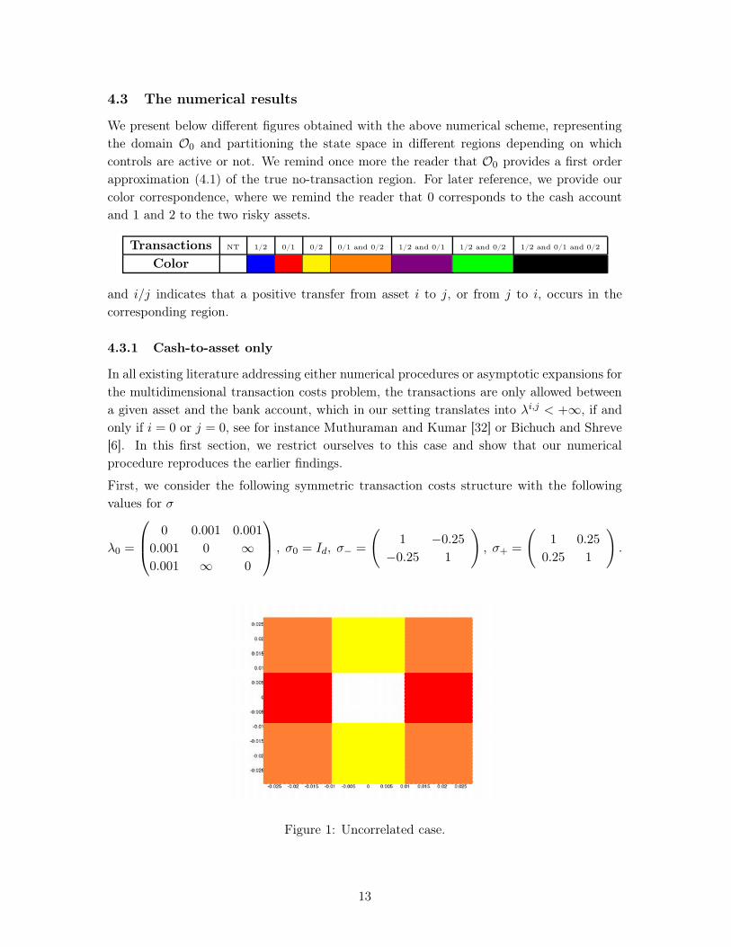
4.3 The numerical results
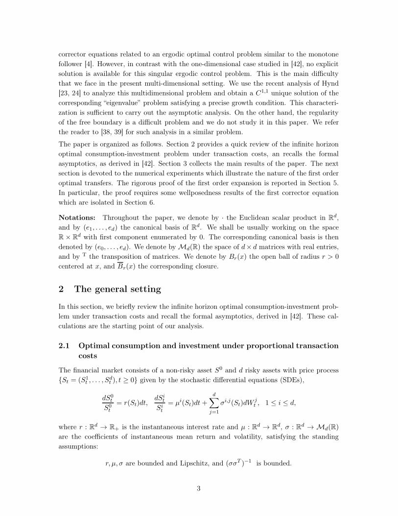
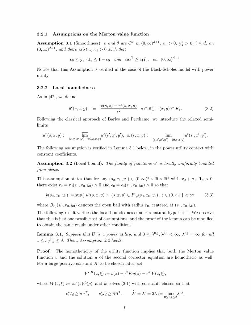
We present below different figures obtained with the above numerical scheme, representingthe domain O0 and partitioning the state space in different regions depending on whichcontrols are active or not. We remind once more the reader that O0 provides a first orderapproximation (4.1) of the true no-transaction region. For later reference, we provide ourcolor correspondence, where we remind the reader that 0 corresponds to the cash accountand 1 and 2 to the two risky assets.
Transactions NT 1/2 0/1 0/2 0/1 and 0/2 1/2 and 0/1 1/2 and 0/2 1/2 and 0/1 and 0/2
Color
and i/j indicates that a positive transfer from asset i to j, or from j to i, occurs in thecorresponding region.
4.3.1 Cash-to-asset only
In all existing literature addressing either numerical procedures or asymptotic expansions forthe multidimensional transaction costs problem, the transactions are only allowed betweena given asset and the bank account, which in our setting translates into λi,j < +∞, if andonly if i = 0 or j = 0, see for instance Muthuraman and Kumar [32] or Bichuch and Shreve[6]. In this first section, we restrict ourselves to this case and show that our numericalprocedure reproduces the earlier findings.
First, we consider the following symmetric transaction costs structure with the followingvalues for σ
λ0 =
⎛⎜⎝ 0 0.001 0.001
0.001 0 ∞0.001 ∞ 0
⎞⎟⎠ , σ0 = Id, σ− =
(1 −0.25
−0.25 1
), σ+ =
(1 0.25
0.25 1
).
Figure 1: Uncorrelated case.
13
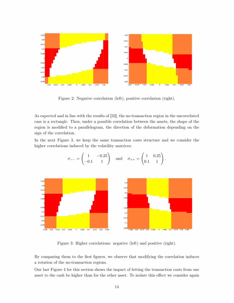
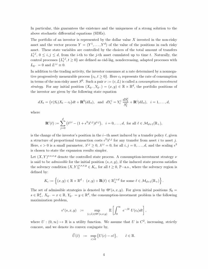
Figure 2: Negative correlation (left), positive correlation (right).
As expected and in line with the results of [32], the no-transaction region in the uncorrelatedcase is a rectangle. Then, under a possible correlation between the assets, the shape of theregion is modified to a parallelogram, the direction of the deformation depending on thesign of the correlation.
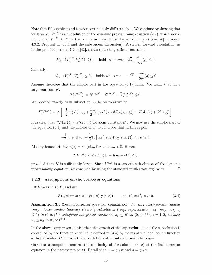
In the next Figure 3, we keep the same transaction costs structure and we consider thehigher correlations induced by the volatility matrices:
σ−− =
(1 −0.25
−0.1 1
)and σ++ =
(1 0.25
0.1 1
).
Figure 3: Higher correlations: negative (left) and positive (right).
By comparing them to the first figures, we observe that modifying the correlation inducesa rotation of the no-transaction regions.
Our last Figure 4 for this section shows the impact of letting the transaction costs from oneasset to the cash be higher than for the other asset. To isolate this effect we consider again
14
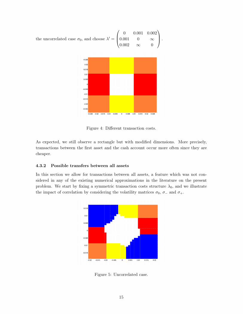
the uncorrelated case σ0, and choose λ′ =
⎛⎜⎝ 0 0.001 0.002
0.001 0 ∞0.002 ∞ 0
⎞⎟⎠ .
Figure 4: Different transaction costs.
As expected, we still observe a rectangle but with modified dimensions. More precisely,transactions between the first asset and the cash account occur more often since they arecheaper.
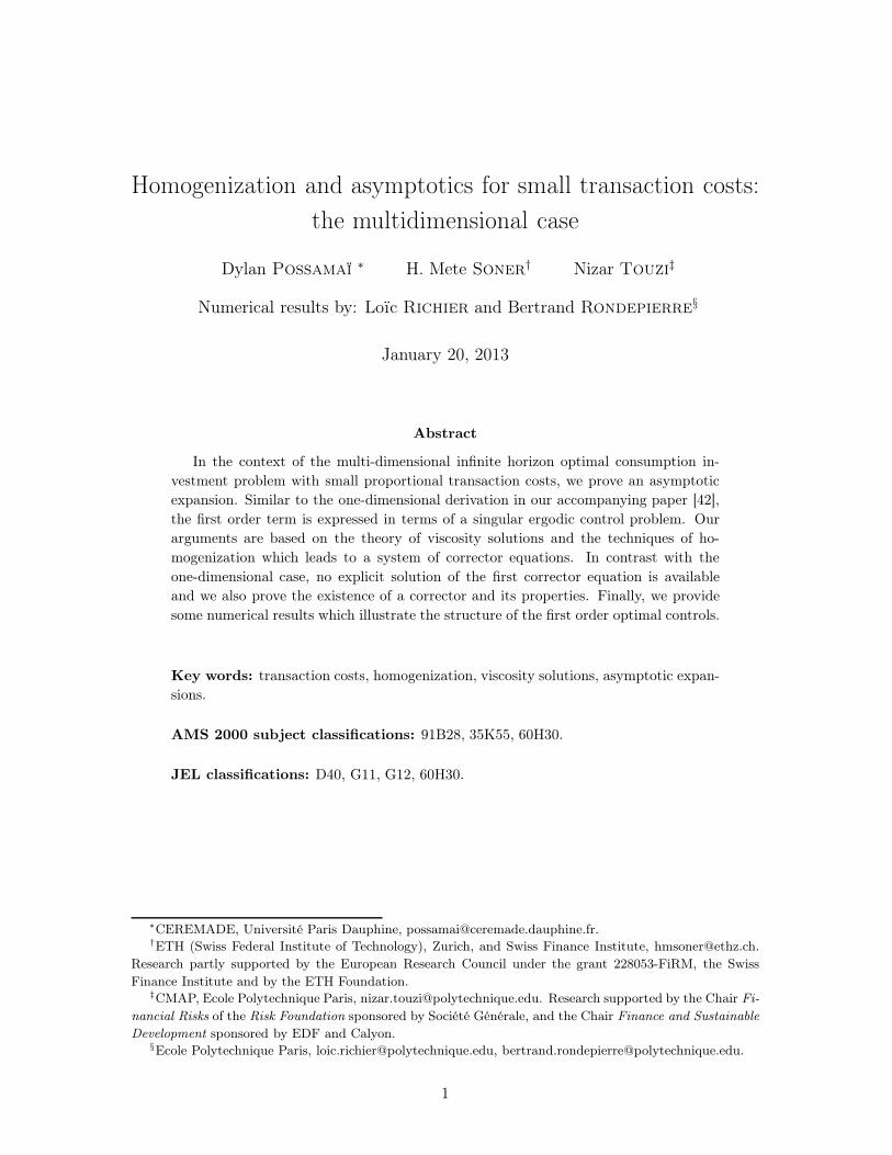
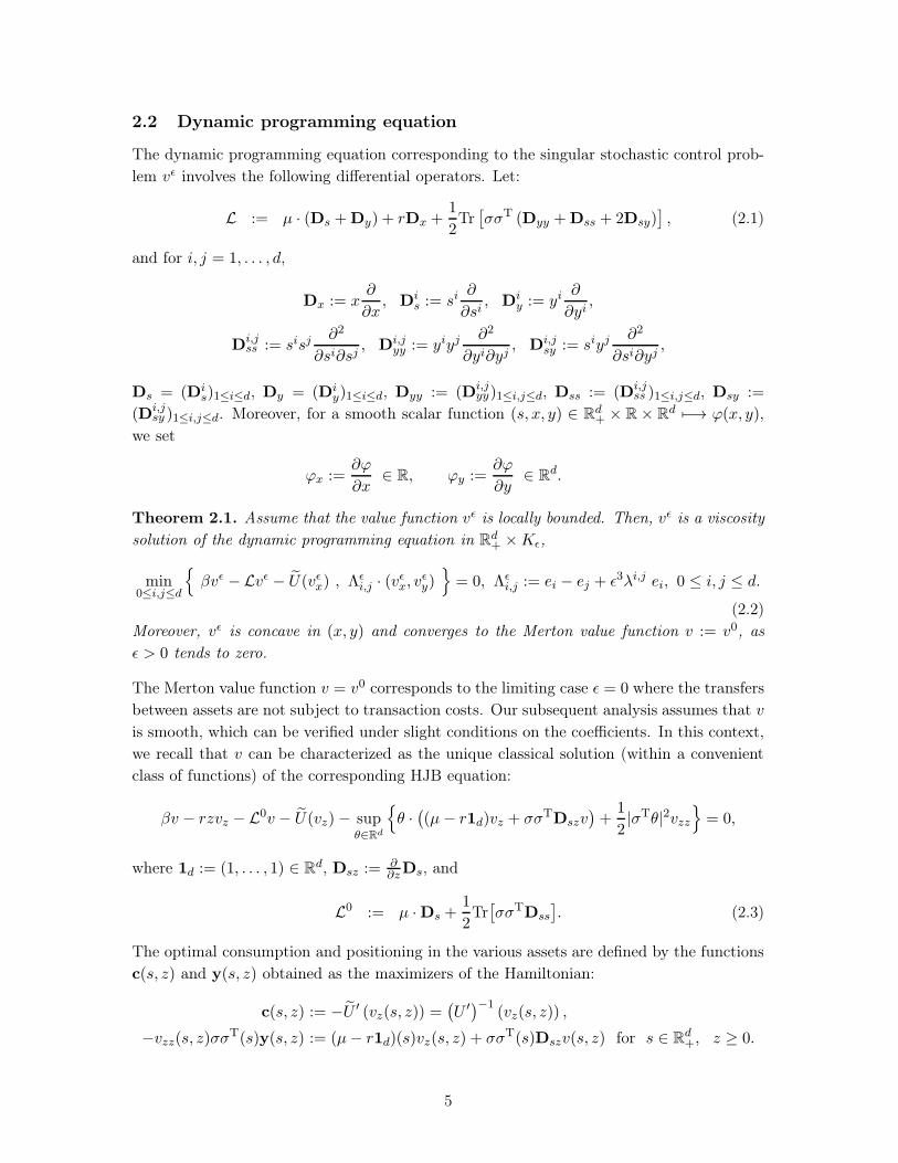
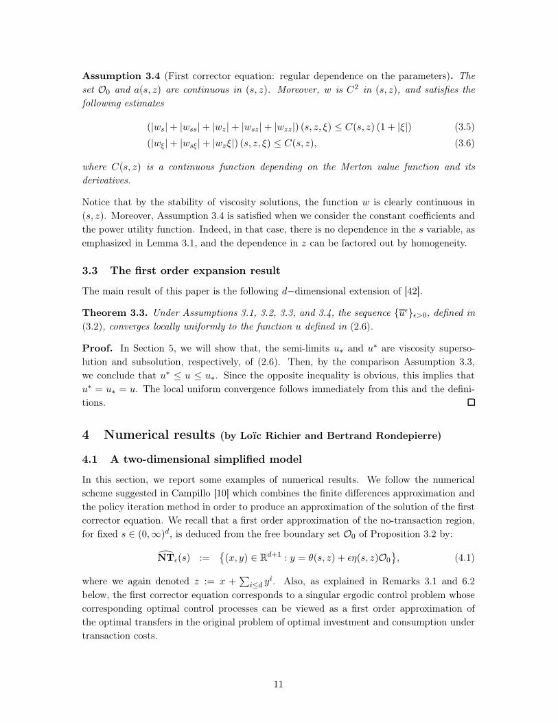
4.3.2 Possible transfers between all assets
In this section we allow for transactions between all assets, a feature which was not con-sidered in any of the existing numerical approximations in the literature on the presentproblem. We start by fixing a symmetric transaction costs structure λ0, and we illustratethe impact of correlation by considering the volatility matrices σ0, σ− and σ+.
Figure 5: Uncorrelated case.
15
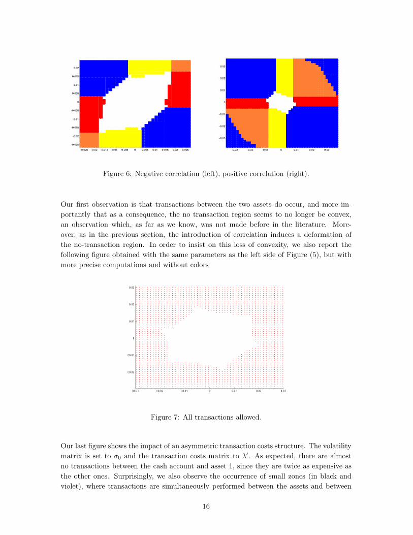
Figure 6: Negative correlation (left), positive correlation (right).
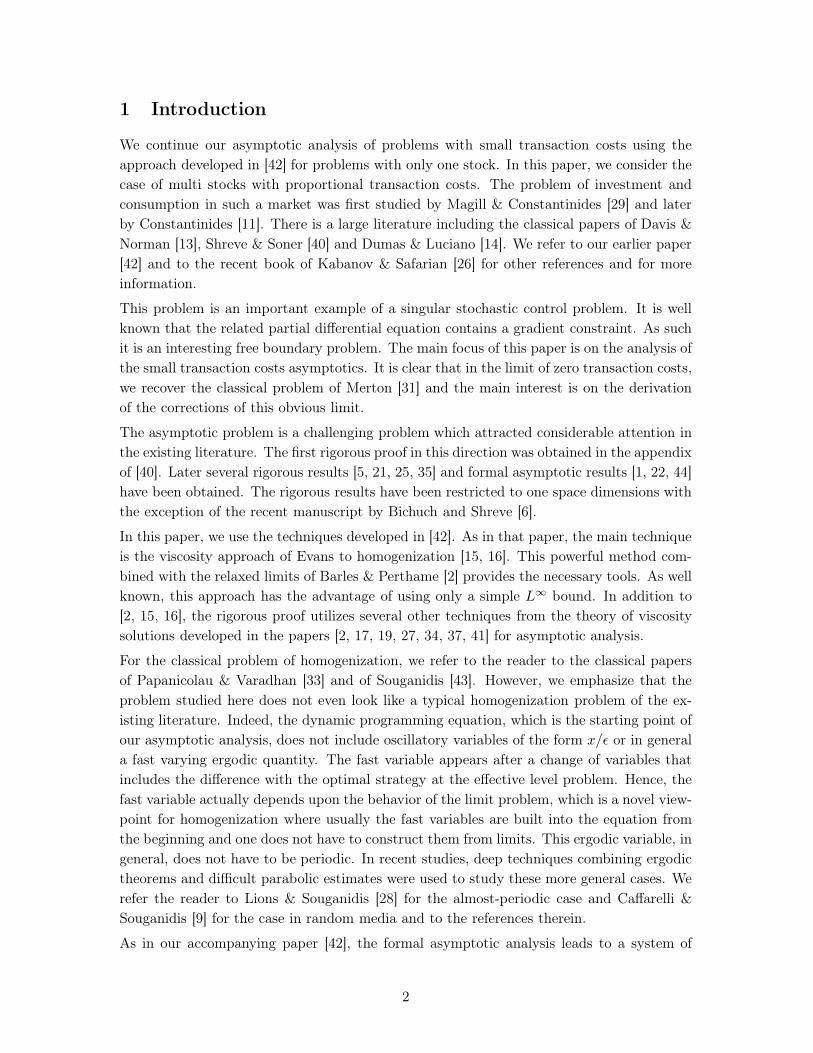
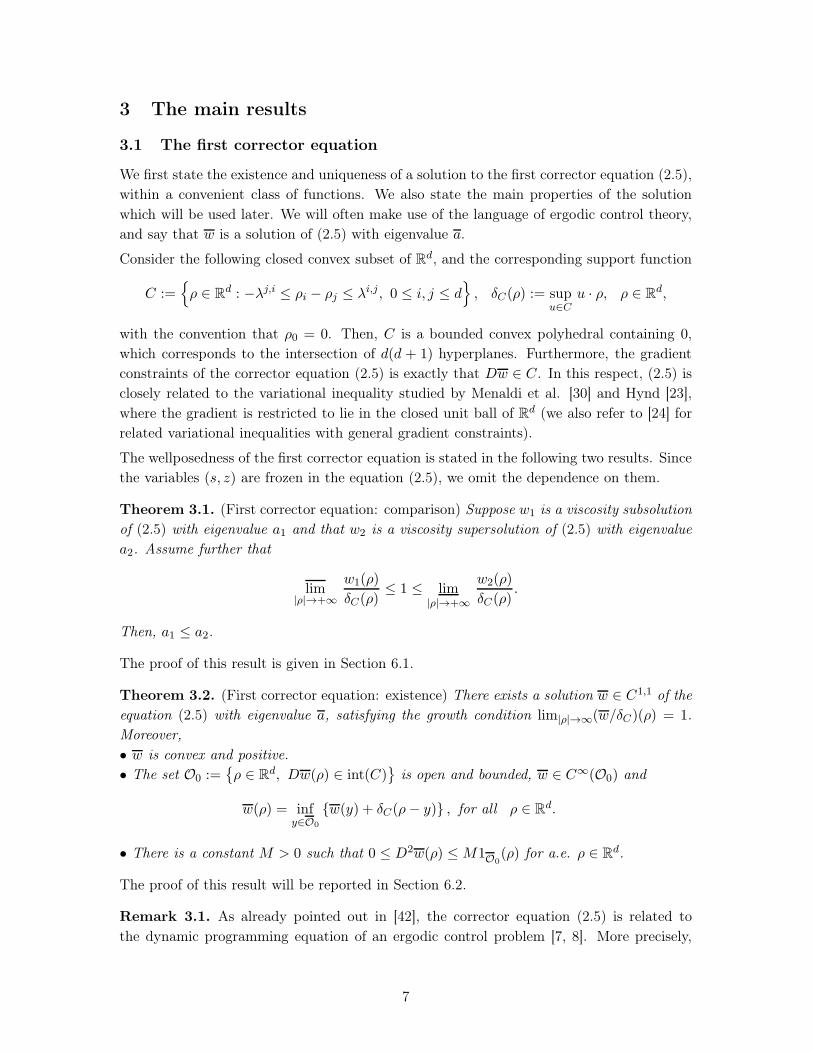
Our first observation is that transactions between the two assets do occur, and more im-portantly that as a consequence, the no transaction region seems to no longer be convex,an observation which, as far as we know, was not made before in the literature. More-over, as in the previous section, the introduction of correlation induces a deformation ofthe no-transaction region. In order to insist on this loss of convexity, we also report thefollowing figure obtained with the same parameters as the left side of Figure (5), but withmore precise computations and without colors
−0.03 −0.02 −0.01 0 0.01 0.02 0.03
−0.02
−0.01
0
0.01
0.02
0.03
Figure 7: All transactions allowed.
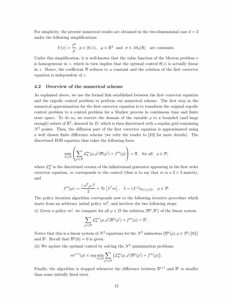
Our last figure shows the impact of an asymmetric transaction costs structure. The volatilitymatrix is set to σ0 and the transaction costs matrix to λ′. As expected, there are almostno transactions between the cash account and asset 1, since they are twice as expensive asthe other ones. Surprisingly, we also observe the occurrence of small zones (in black andviolet), where transactions are simultaneously performed between the assets and between
16

the assets and the cash account.
Figure 8: Asymmetric transaction costs.
5 Convergence
In the rest of the paper, we denote for any function f(s, x, y):
f(s, z, ξ) := f(s, z − y(s, z) · 1d, εξ + y(s, z)
).
This section is dedicated to the proof of our main result, Theorem 3.3. Let:
uε(s, x, y) := uε(s, x, y)− ε2w(s, z, ξ), s ∈ Rd+, (x, y) ∈ Kε.
5.1 First estimates and properties
We start by obtaining several estimates of uε. Set
λ := max0≤i,j≤d
λi,j, λ := min0≤i,j≤d
λi,j.
We also recall that L is the upper bound of the set C.
Lemma 5.1. For (ε, s, x, y) ∈ (0,+∞) × (0,+∞)d ×Kε, and z := x+ y, we have
uε(s, x, y) ≥ −εLvz(s, z) |y − y(s, z)| .Consequently, under Assumption 3.2, we have for all (ε, s, x, y) ∈ (0,+∞)× (0,+∞)d ×Kε
0 ≤ u∗(s, x, y) ≤ u∗(s, x, y) < +∞.
Proof. Since vε(s, x, y) ≤ v(s, z), it follows from the definition of uε that
uε(s, x, y) ≥ −ε2w(s, z, ξ).Next, recall that Dw takes values in the bounded set C. Since w(., 0) = 0, this implies that−w(s, z, ξ) ≥ −L |ξ| vz(s, z), and completes the proof.
The next Lemma proves that the relaxed semi-limits are only functions of (s, z).
17
Lemma 5.2. Let Assumptions 3.1 and 3.2 hold. Then, u∗ and u∗ are only functions of(s, z). Furthermore, we have
u∗(s, z) = lim(ε,s′,z′)→(0,s,z)
uε(s′, z′ − y(s′, z′) · 1d,y(s′, z′)
)u∗(s, z) = lim
(ε,s′,z′)→(0,s,z)uε(s′, z′ − y(s′, z′) · 1d,y(s′, z′)
).
Proof. We proceed in several steps. We assume throughout the proof that the parameterε is less than one.
Step 1: In view of the gradient constraints of the dynamic programming equation satisfiedby vε, we know that for all 1 ≤ i ≤ d, we have in the viscosity sense
Λεi,0.(v
εx, v
εy) ≥ 0, Λε
0,i.(vεx, v
εy) ≥ 0. (5.1)
Now definevε(s, z, ξ) := vε(s, z − εξ · 1d − y(s, z) · 1d, εξ + y(s, z)).
We directly calculate that (5.1) implies for all 1 ≤ i ≤ d in the viscosity sense
ε4λi,0vεz(s, z, ξ) − ε3λi,0yz(s, z).vεξ(s, z, ξ) + (1 + ε3λi,0)vεξi(s, z, ξ) ≥ 0, (5.2)
andε4λ0,ivεz(s, z, ξ) − ε3λ0,iyz(s, z).v
εξ(s, z, ξ) − vεξi ≥ 0. (5.3)
Using the fact that all the yiz(s, z) are strictly positive (see Assumption 3.1), we can multiply
(5.2) by yiz(s, z) and sum to obtain, once more in the viscosity sense(
1− ε3d∑
i=1
yiz(s, z)λ
i,0
1 + ε3λi,0
)yz(s, z).v
εξ(s, z, ξ) ≥ −ε4
d∑i=1
λi,0
1 + ε3λi,0vεz(s, z, ξ). (5.4)
Now, we have by Assumption 3.1
1− ε3d∑
i=1
yiz(s, z)λ
i,0
1 + ε3λi,0= 1−
d∑i=1
yiz(s, z) +
d∑i=1
yiz(s, z)
1 + ε3λi,0≥ 0.
Using this inequality in (5.4) yields, in the viscosity sense
yz(s, z).vεξ(s, z, ξ) ≥ −
∑di=1
λi,0
1+ε3λi,0
1− ε3∑d
i=1yiz(s,z)λ
i,0
1+ε3λi,0
ε4vεz(s, z, ξ). (5.5)
Plugging this estimate in (5.2) and (5.3), we obtain in the viscosity sense
vεξi(s, z, ξ) ≤ λ0,iε4
(1 +
∑di=1
λi,0
1+ε3λi,0
1− ε3∑d
i=1yiz(s,z)λ
i,0
1+ε3λi,0
)vεz(s, z, ξ) ≤ ε4λ
(1 +
λd
c0
)vεz(s, z, ξ),
andvεξi(s, z, ξ) ≥ −2ε4λvεz(s, z, ξ).
18
By the concavity of vε, its gradient exists almost everywhere. Moreover, since we assumedthat y is smooth, this implies that vεz also exists almost everywhere. Hence, we concludefrom the above estimates that∣∣vεξ∣∣ ≤ Aε4vεz, where A :=
√dmax
{λ(1 +
λ2d
c0
), 2λ}. (5.6)
Step 2: We now prove an estimate for vεz. By definition and from Assumption 3.1,
vεz(s, z, ξ) = ∂zvε (s, z − εξ · 1d − y(s, z) · 1d, εξ + y(s, z))
= (1− yz(s, z) · 1d) vεx(s, x, y) + yz(s, z).vεy(s, x, y)
≤ vεx(s, x, y) + vεy(s, x, y) · 1d. (5.7)
Therefore, we can focus on obtaining estimates on vεx and vεy. First, by concavity of vε in xand of v in z, we have
vεx(s, x, y) ≤vε(s, x, y)− vε(s, x− ε, y)
ε
≤ v(s, z)− v(s, z − ε)
ε+v(s, z − ε)− vε(s, x− ε, y)
ε
≤ vz(s, z − ε) +v(s, z − ε)− vε(s, x− ε, y)
ε.
Now, using the definition of uε, we obtain
vεx(s, x, y) ≤ vz(s, z − ε) + ε(uε(s, x− ε, y) + ε2w(s, z − ε, ξε)
),
whereξε :=
y − y(s, z − ε)
ε= ξ +
y(s, z) − y(s, z − ε)
ε.
From the estimates on w in Theorem 3.1 and Assumption 3.4, we have
|w(s, z − ε, ξε)| ≤ Lvz(s, z)(1 + |ξε|) ≤ Lvz(s, z)
(1 + |ξ|+ |y(s, z) − y(s, z − ε)|
ε
),
and therefore
vεx(s, x, y) ≤ vz(s, z − ε) + εuε(s, x− ε, y) + ε3Lvz(s, z)
(1 + |ξ|+ |y(s, z) − y(s, z − ε)|
ε
).
As for vεy, we use again the concavity of vε and v in y and z, respectively,
vεyi(s, x, y) ≤vε(s, x, y)− vε(s, x, y − εei)
ε
≤ v(s, z) − v(s, z − ε)
ε+v(s, z − ε)− vε(s, x, y − εei)
ε
≤ vz(s, z − ε) +v(s, z − ε)− vε(s, x, y − εei)
ε, 0 ≤ i ≤ d.
Similarly as above, this yields
vεyi(s, x, y) ≤ vz(s, z − ε) + εuε(s, x, y − εei)
+ε3Lvz(s, z)
(1 + |ξ|+ |−εei + y(s, z) − y(s, z − ε)|
ε
).
19
Plugging the above estimates in (5.7), we get
vεz(s, z, ε) ≤(1 + d)vz(s, z − ε) + ε
(uε(s, x− ε, y) +
d∑i=1
uε(s, x, y − εei)
)(5.8)
+ ε3Lvz(s, z)
(d+ (1 + d)
(1 + |ξ|+ |y(s, z) − y(s, z − ε)|
ε
))=: γε(s, z, ξ).
Step 3 Recall that vεz exists almost everywhere, and thus by definition of uε, this also holdsfor uεz and uεξ. Now, using (5.6), (5.8) together with Assumption 3.1 and our estimates onw, we obtain for some constant C > 0∣∣uεξ(s, z, ξ)∣∣ ≤ ε2C (vz(s, z) + vεz(s, z, ξ)) ≤ ε2C (vz(s, z) + γεz(s, z, ξ)) .
With this estimate, we can conclude the proof exactly as in the proof of Lemma 6.2 in[42].
5.2 Remainder estimate
In this section, we isolate an estimate which will be needed at various occasions in thesubsequent proofs. The following calculation extends the estimate of Section 4.2 in [42].For any function
Ψε(s, x, y) := v(s, z)− ε2φ(s, z) − ε4�(s, z, ξ),
with smooth φ and υ such that υ also verifies the estimates (3.5), we have
I(Ψε)(s, x, y) : =(βΨε − LΨε − U(Ψε
x))(s, x, y)
= ε2[−1
2|σ(s)ξ| vzz + 1
2Tr[ααT (s, z)�ξξ(s, z, ξ)
]−Aφ(s, z) +Rε(s, z, ξ)
].
Similarly as in [42], direct but tedious calculations provides the following estimate:
|Rε(s, x, y)| ≤ε(|μ− r · 1d| |ξ| |φz|+ |σ|2
2
(2 |y| |ξ|+ εξ2
) |φzz|+ |σ|2 |ξ| |Dszφ|)(s, z)
+ εC(s, z)(1 + ε |ξ|+ ε2 |ξ|2 + ε3 |ξ|3
)+ ε−2
∣∣∣U(Ψεx)− U(vz)− (Ψε
x − vz)U′(vz)
∣∣∣ ,for some continuous function C(s, z). Now using the fact U is C1 and convex and theestimates assumed for υ, we obtain
|Rε(s, x, y)| ≤ε(|μ− r · 1d| |ξ| |φz|+ |σ|2
2
(2 |y| |ξ|+ εξ2
) |φzz|+ |σ|2 |ξ| |Dszφ|)(s, z)
+ εC(s, z)(1 + ε |ξ|+ ε2 |ξ|2 + ε3 |ξ|3
)+ ε2 (|φz|+ εC(s, z)(1 + ε |ξ|))2 U ′′ (
vz + ε2 |φz|+ ε3C(s, z)(1 + ε |ξ|)) .
20
5.3 Viscosity subsolution property
In this Section, we prove
Proposition 5.1. Under Assumptions 3.1, 3.2 and 3.4, the function u∗ is a viscosity sub-solution of the second corrector equation.
Proof. Let (s0, z0, φ) ∈ (0,+∞)d × (0,+∞)× C2((0,+∞)d × (0,+∞)
)be such that
(u∗ − φ)(s0, z0) > (u∗ − φ)(s, z), for all (s, z) ∈ (0,+∞)d × (0,+∞)\ {(s0, z0)}. (5.9)
By definition of viscosity subsolutions, we need to show that
Aφ(s0, z0)− a(s0, z0) ≤ 0.
We will proceed in several steps.
Step 1: First of all, we know from Lemma 5.2 that there exists a sequence (sε, zε) whichrealizes the lim sup for uε, that is to say
(sε, zε) −→ε↓0
(s0, z0) and uε(sε, zε, 0) −→ε↓0
u∗(s0, z0).
It follows then easily that lε∗ := uε(sε, zε, 0)− φ(sε, zε) −→ε↓0
0, and
(xε, yε) = (zε − y(sε, zε) · 1d,y(sε, zε)) −→ε↓0
(x0, y0) := (z0 − y(s0, z0) · 1d,y(s0, z0)) .
Now recall from Assumption 3.2 that uε is locally bounded from above. This implies theexistence of r0 := r0(s0, x0, y0) > 0 and ε0 := ε0(s0, x0, y0) > 0 verifying
b∗ := sup {uε(s, x, y), (s, x, y) ∈ B0, ε ∈ (0, ε0]} < +∞, (5.10)
where B0 := Br0(s0, x0, y0) is the open ball with radius r0 and center (s0, x0, y0). Moreover,notice that we can always decrease r0 so that r0 ≤ z0/2, which then implies that B0 doesnot cross the line z = 0. Now for any (ε, δ) ∈ (0, 1]2, we define Ψε,δ and the correspondingΨε,δ by
Ψε,δ(s, z, ξ) := v(s, z)− ε2(lε∗ + φ(s, z) + Φε(s, z, ξ)
)− ε4(1 + δ)w(s, z, ξ),
where the function Φε and the corresponding Φε are given by:
Φε(s, x, y) := c0
((s− sε)4 + (z − zε)4 + ε4w4(s, z, ξ)
),
and c0 > 0 is a constant chosen large enough in order to have for ε small enough
Φε ≤ 1 + b∗ − φ, on B0\B1, where B1 := B r02(s0, x0, y0). (5.11)
We emphasize that the constant c0 may depend on (φ, s0, x0, y0, δ) but not on ε, and thata priori the function Ψε,δ is not C2 in ξ, because the function w is only in C1,1. This is amajor difference with the one-dimension case treated in [42].
21

Step 2: We now prove that for all sufficiently small ε and δ, the difference (vε − Ψε,δ) hasa local minimizer in B0. First, notice that this is equivalent to showing that the followingquantity has a local minimizer in B0
Iε,δ(s, x, y) : =vε(s, x, y)−Ψε,δ(s, x, y)
ε2
= −uε(s, x, y) + lε∗ + φ(s, z) + φε(s, x, y) + ε2δw(s, z, ξ).
By (5.11) and the fact that w ≥ 0, we have for any (s, x, y) ∈ ∂B0
Iε,δ(s, x, y) ≥ −uε(s, x, y) + lε∗ + 1 + b∗ + ε2δw(s, z, ξ) ≥ 1 + lε∗ > 0,
for ε small enough. Moreover, since Iε,δ(sε, xε, yε) = 0, this implies that Iε,δ has a localminimizer (sε, xε, yε) in B0, and we introduce the corresponding
zε := xε + yε · 1d, and ξε :=yε − y(sε, zε)
ε.
We then have
min(s,z,ξ)
(vε − Ψε,δ)(s, z, ξ) = (vε −Ψε,δ)(sε, zε, ξε) ≤ 0, |sε − s0|+ |zε − z0| ≤ r0,∣∣∣ξε∣∣∣ ≤ r1
ε,
for some constant r1. We now use the viscosity supersolution property of vε. Since Ψε,δ isC1, we obtain from the first order operator in the dynamic programming equation that:
Λεi,j ·
(Ψε,δ
x ,Ψε,δy
)(sε, xε, yε) ≥ 0 for all 0 ≤ i, j ≤ d. (5.12)
Step 3: In this step, we show that for ε small enough, we have
ρε :=ξε
η(sε, zε)∈ O0(s
ε, zε). (5.13)
where O0(s, z) is the open set of Proposition 3.2. We argue by contradiction assuming thatthere exists some sequence εn −→ 0 such that ρεn �∈ O0(s
εn , zεn). This implies that
−λin0 ,jn0 +(∂in0w − ∂jn0 w
)(sεn , zεn , ρεn) = 0 for some (in0 , j
n0 ). (5.14)
By the gradient constraint (5.12), and the boundedness of(sεn , zεn , εnξ
εn)n, we directly
compute that:
− 4Cε2n(εnw)3(sεn , zεn , ξεn)
(wξi
n0− w
ξjn0
)(sεn , zεn , ξεn)
+ ε3nvz(sεn , zεn)
[λi
n0 ,j
n0 − (1 + δ)(∂in0w − ∂jn0 w)(s
εn , zεn , ρεn)]+ ◦(ε3n) ≥ 0. (5.15)
Using (5.14) and the non-negativity of w, this implies
0 ≤ −4c0λin0 ,j
n0 ε2n(εnw)
3(sεn , zεn , ξεn)− δλin0 ,j
n0 ε3nvz(s
εn , zεn) + ◦(ε3n)≤ −δλin0 ,jn0 ε3nvz(sεn , zεn) + ◦(ε3n) ≥ 0,
which leads to a contradiction when n goes to +∞.
22
Step 4: From (5.13) and Proposition 3.2, we deduce that in our domain of interest, thefunction Ψε,δ is actually smooth, and is therefore a legitimate test function for the second or-der operator of the dynamic programming equation. We then obtain from the supersolutionproperty of vε that (
βvε − LΨε,δ − U(Ψε,δx ))(sε, xε, yε) ≥ 0. (5.16)
Moreover, by Step 3 and the continuity of (s, z) �−→ O(s, z) in Assumption 3.4, the sequence(ξε)ε is bounded. By classical results in the theory of viscosity solutions, there exists asequence εn → 0 and some ξ such that
(sn, zn, ξn) := (sεn , zεn , ξεn) −→ (s0, z0, ξ).
Now recall that the function w is smooth in this case and that the function Ψε,δ has exactlythe form given in Section 5.2. By the remainder estimate in (5.16), we obtain
1
2η(sn, zn) |σ(sn)ξn|2+1
2(1+δ)Tr
[ααT (sn, zn)wξξ(sn, zn, ξn)
]−Aφ(sn, zn)+Rε(s, z, ξ) ≥ 0.
We still have no guarantee that w is C2 at ξ. Therefore, we carefully estimate the terminvolving wξξ. Indeed, the equation satisfied by w yields
a(sn, zn)−Aφ(sn, zn) + δ
(a(sn, zn)− 1
2η(sn, zn) |σ(sn)ξn|2
)+Rε(s, z, ξ) ≥ 0. (5.17)
Notice that the estimate on the remainder of Section 5.2 still hold true if terms involvingwξξ are replaced by means of the first corrector equation. Since the map (s, z) �−→ a(s, z) iscontinuous, by Assumption 3.4, and all derivatives of Φε vanish at the origin, we may sendε to 0 in (5.17) and obtain
a(s0, z0)−Aφ(s0, z0) + δ
(a(s0, z0)− 1
2η(s0, z0)|σ(s0)ξ|2
)≥ 0. (5.18)
Since ξ is bounded uniformly in δ, we let δ go to zero in (5.18) to obtain the desiredresult.
5.4 Viscosity supersolution property
In this section we will prove the following result.
Proposition 5.2. Under Assumptions 3.1, 3.2 and 3.4, u∗ is a viscosity supersolution ofthe second corrector equation.
To prove this result, we start by two useful lemmas. For the first one, we recall that in theproof of the viscosity subsolution property in the previous section, we mentioned that thefunction w is not C2 in the whole space. We overcome this difficulty by using the fact thatwe only needed w on a subset of Rd where it is actually smooth. However, in the proof of theviscosity supersolution property, we need w to be defined on the whole space. Therefore, wemollify it and the following Lemma gives some useful properties satisfied by this mollifiedversion of w.
23

Let k : Rd → R be a positive, even (i.e. k(−x) = k(x) for all x ∈ Rd), C∞ function with
support in the closed unit ball of Rd and unit total mass. For all m > 0, we define
km(x) :=1
mdk( ξm
)and wm(s, z, ξ) :=
∫Rd
km(ζ)w(ξ − ζ)dζ −∫Rd
km(ζ)w(−ζ)dζ.
Lemma 5.3. Let Assumption 3.4 hold. For any m > 0, the function wm satisfies:(i) wm is C2, convex in ξ, and we have for all 0 ≤ i, j ≤ d
wmξi (s, z, ξ) =
∫Rd
km(ζ)wξi(s, z, ξ − ζ)dζ, wmξiξj (s, z, ξ) =
∫Rd
km(ζ)wξiξj(s, z, ξ − ζ)dζ.
Moreover, 0 ≤ wm(s, z, ξ) ≤ Lvz(s, z) |ξ| .(ii) wm is smooth in (s, z), and satisfies the following estimates, uniformly in m,
(|wm|+ |wms |+ |wm
ss|+ |wmz |+ |wm
sz|+ |wmzz|) (s, z, ξ) ≤ C(s, z) (1 + |ξ|)(∣∣wm
ξ
∣∣+ ∣∣wmsξ
∣∣+ ∣∣wmzξ
∣∣) (s, z, ξ) ≤ C(s, z)∣∣wmξξ(s, z, ξ)
∣∣ ≤ C(s, z)1ξ∈B(s,z), (5.19)
where C(s, z) is a continuous function depending on the Merton value function and itsderivatives, and B(s, z) is small ball with continuous radius and center in (s, z).
(iii) For every 0 ≤ i, j ≤ d and every (s, z, ξ)
−λi,jvz(s, z) + wmξi (s, z, ξ) − wm
ξj (s, z, ξ) ≤ 0.
(iv) For every (s, z, ξ), we have
1
2vzz(s, z)
∫Rd
km(x) |σ(s)(ξ − ζ)|2 dζ − 1
2Tr[ααT (s, z)wm
ξξ(s, z, ξ)]+ a(s, z) ≤ 0.
Proof. (i) The fact that wm is C2 in ξ is a classical result. Moreover, we have by definitionwm(s, z, 0) = 0 and by convexity of w, we have wm ≥ w ≥ 0. The equalities for thederivatives of wm follow from the fact that w is C1 in ξ and C2 almost everywhere. Finally,wm inherits clearly the convexity and Lipschitz property of w.
(ii) is clear by linearity of the convolution and Assumption 3.4. (iii) is again a consequenceof the linearity of the convolution and the gradient constraints satisfied by w. Finally (iv)
follows from the linearity of the convolution, the second corrector equation satisfied by w
and the formula for wmξξ given in (i).
We next constructs a useful function which plays a major role in our subsequent proof.
Lemma 5.4. For any δ ∈ (0, 1), there exists aδ > 1 and a function hδ : Rd → [0, 1] suchthat hδ is C∞, hδ = 1 on B1(0) and hδ = 0 on Baδ(0)
c. Moreover, for any 1 ≤ i ≤ d andfor any ξ ∈ R
d ∣∣∣hδξi(ξ)∣∣∣ ≤ δ
2Lλ1B
aδ(0)(ξ), and |ξ| |hδξξ| ≤ C∗,
for some constant C∗ independent of δ.
24
Proof. Let φ be an even C∞ function on R+, whose support is in (−1, 1), such that0 ≤ φ ≤ 1 and
∫ 1−1 φ(t)dt = 1. For some α > 0 to be specified later, we define the following
function hα : R+ −→ [0, 1]:
hα(x) :=
∫ 1
−1Hα(x− t)φ(t)dt, where Hα(x) := 1{x≤2} +
(1− α ln
(x2
))1{2<x≤2e1/α}.
Clearly, hα is C∞, hα = 1 on [0, 1] and to hα = 0 for [1 + 2e1/α,∞). Moreover, hα isdecreasing and its derivative clearly verifies for every x ∈ R
0 ≥ h′α(x) ≥ −α2. (5.20)
We claim that ∣∣∣xh′′α(x)∣∣∣ ≤ 3α
4for all x ∈ R. (5.21)
Indeed, this inequality is obvious on (−∞, 1], and we compute for x ≥ 1, that
0 ≤ xh′′α(x) =∫ 1
−1
αx
(x− t)21{2<x−t≤2e1/α}φ(t)dt ≤
∫ 1
−1α3
4φ(t)dt =
3α
4.
We now introduce the function:
hδ(ξ) := hδ (|ξ|) , δ :=δ
Lλξ ∈ R
d.
Clearly hδ is C∞, takes values in [0, 1], hδ = 1 on B0(1), and hδ = 0 on B1+2eL/δ(0)c. Inparticular, this provides the existence of aδ ∈ [1, 1 + 2e
Lδ ]. Also
hδξi(ξ) = h′δ(|ξ|) ξi|ξ| .
Thus, by (5.20) and the fact that hδ and all its derivatives vanish on (aδ,∞):∣∣∣hδξi(ξ)∣∣∣ ≤ δ
2Lλ1B
aδ(0)(x).
Similarly, we have
|ξ| hδξξ(ξ) =(|ξ| h′′
δ(|ξ|)− 1
2h′δ(|ξ|)
)ξξT|ξ|2 + h′
δ(|ξ|)Id.
Consequently, using (5.20), (5.21), and the fact that δ ∈ (0, 1), we have for some constantC which only depends on the dimension d:
|ξ| ∣∣hδξξ∣∣ ≤ C
(3δ
4Lλ+
δ
4Lλ+
δ
2Lλ
)≤ 3C
2Lλ.
Proof. [Proposition 5.2] Let (s0, z0, φ) ∈ (0,+∞)d+1 × C2((0,+∞)d+1
)be such that
(u∗ − φ)(s0, z0) < (u∗ − φ)(s, z), for all (s, z) ∈ (0,+∞)d × (0,+∞)\ {(s0, z0)}. (5.22)
25

By the definition of viscosity supersolutions, we need to show that
Aφ(s0, z0)− a(s0, z0) ≥ 0. (5.23)
We argue by contradiction and assume that
Aφ(s0, z0)− a(s0, z0) < 0. (5.24)
Then by the continuity of φ and a, for some r0 > 0, we will have
Aφ(s, z)− a(s, z) ≤ 0 on Br0(s0, z0) for some r0 > 0. (5.25)
Step 1: This first step is devoted to defining the test function we will consider in the sequel.First of all, we know from Lemma 5.2 that there exists a sequence (sε, zε) which realizes thelim for uε, that is to say
(sε, zε) −→ε↓0
(s0, z0) and uε(sε, zε, 0) −→ε↓0
u∗(s0, z0).
It follows then easily that lε∗ := uε(sε, zε, 0)− φ(sε, zε) −→ε↓0
0, and
(xε, yε) = (zε − y(sε, zε) · 1d,y(sε, zε)) −→ε↓0
(x0, y0) := (z0 − y(s0, z0) · 1d,y(s0, z0)) .
We then choose ε0, depending on z0, s0 and φ, such that for all ε ≤ ε0, we have
|zε − z0| ≤ r04, |sε − s0| ≤ r0
4, |l∗ε | ≤ 1. (5.26)
By the continuity of φ and vz, we may also introduce a constant c0 > 0 such that
sup(s,z)∈Br0/2
(s0,z0)
{φ(s, z) + vz(s, z)}+ 3 ≤ 2c0
(r04
)4. (5.27)
Notice that since φ and vz are continuous, the supremum on the compact set B(s0, z0, r0/2)above is indeed finite. This justifies the existence of c0. We now define
ϕε(s, z) := φ(s, z)− c0
(|z − zε|4 + |s− sε|4
).
Then, for all ε ≤ ε0 and for any (s, z) ∈ Br0/2(s0, z0), we have using (5.27) and (5.26)
ϕε(s, z) + l∗ε + vz(s, z) = φ(s, z) + vz(s, z)− c0
(|z − zε|4 + |s− sε|4
)+ l∗ε
≤ 2c0
(r04
)4 − 3− c0
(|z − zε|4 + |s− sε|4
)+ 1
≤ c0
(2(r04
)4− |z − zε|4 − |s− sε|4
)− 2 ≤ −2, (5.28)
whenever (s, z) ∈ ∂Br0/2(s0, z0).
Before defining our final test function, we provide another parameter. Let ξ0 > 0 be greaterthan the diameter of the open bounded set O0(s0, z0), and fix some ξ∗ ≥ 1 ∨ ξ0 ∨ ξ∗ where
ξ∗ := sup(s,z)∈B(s0,z0,r0/2)
⎛⎝1 + 2a(s, z) + C∗+λ−1
2 Tr[ααT (s, z)
]vz(s, z)
12 |σ|2 (−vzz)(s, z)
⎞⎠1/2
,
26
and C∗ is the constant appearing in Lemma 5.4(iv). Then, for any ξ ∈ Bξ∗(0)c, it follows
from (5.25) that for any (s, z) ∈ Br0/2(s0, z0):
1
2|σξ|2 (−vzz)(s, z)− C∗ + λ
−1
2Tr[ααT
]vz(s, z)−Aφ(s, z) > 1 + 2a(s, z)−Aφ(s, z) > 1.
(5.29)
Finally, for δ ∈ (0, 1) and m > 0, let hδ be the function introduced in Lemma 5.4, wm thefunction introduced in Lemma 5.3, and define the C2 test function ψε,δ,m(s, x, y) and thecorresponding ψε,δ,m(s, z, ξ) by
ψε,δ,m(s, z, ξ) := v(s, z)− ε2ϕε(s, z)− ε2l∗ε − ε4(1− δ)wm(s, z, ξ)H(ξ), H(ξ) := hδ(ξ
ξ∗
).
Step 2: In this step, we modify the test function once again in order to recover the interiormaximizer property. We first compute that:
Iε,δ,m(s, z, ξ) := ε−2(vε − ψε,δ,m
)(s, z, ξ)
= φε(s, z)− uε(s, z, ξ) + l∗ε − ε2 [1− (1− δ)H (ξ)]wm(s, z, ξ). (5.30)
In particular, this implies
Iε,δ,m(sε, zε, 0) = φ(sε, zε)− uε(sε, zε, 0) + l∗ε = 0. (5.31)
Furthermore, since vε ≤ v, we also have easily
Iε,δ,m(s, z, ξ) ≤ ϕε(s, z) + l∗ε + ε2(1− δ)H(ξ)wm(s, z, ξ). (5.32)
Now, we use the fact that
0 ≤ δ ≤ 1, vz(s, z) > 0, 0 ≤ H(ξ) ≤ 1|ξ|≤aδξ∗ and 0 ≤ wm(s, z, ξ) ≤ Lvz(s, z) |ξ| ,
in (5.32) to obtain
Iε,δ,m(s, z, ξ) ≤ ϕε(s, z) + l∗ε + ε2L(1− δ)H(ξ)vz(s, z) |ξ|≤ ϕε(s, z) + l∗ε + ε2Lvz(s, z)a
δξ∗ ≤ ϕε(s, z) + l∗ε + vz(s, z), (5.33)
provided that ε ≤ εδ := (Laδξ∗)−1/2.
Define the set Qs0,z0 :={(s, z, ξ), (s, z) ∈ Br0(s0, z0)
}. Let us then distinguish two cases.
First, we assume that (s, z, ξ) ∈ ∂Qs0,z0 for every ξ. Then, if we take ε ≤ ε0 ∧ εδ, using(5.28) and (5.33), we obtain that for any ξ
Iε,δ,m(z, ξ) ≤ −2. (5.34)
We assume next that (s, z, ξ) ∈ int (Qs0,z0). Then, once again for ε ≤ εδ ∧ ε0, we have
Iε,δ,m(z, ξ) ≤ ϕε(s, z) + l∗ε + vz(s, z) ≤ C(s0, z0) < +∞, (5.35)
27

for some constant C(s0, z0) depending only on φ, s0 and z0, since (s, z) lies in a compactset, l∗ε ≤ 1 and all the functions appearing on the right-hand side of (5.35) are continuous.This implies that
ν(ε, δ,m) := sup(s,z,ξ)∈Qs0,z0
Iε,δ,m(s, z, ξ) < +∞.
By definition, we can therefore for each n ≥ 1 find (sn, zn, ξn) ∈ int (Qs0,z0) such that
Iε,δ,m(sn, zn, ξn) ≥ ν(ε, δ,m) − 1
2n. (5.36)
Since we have no guarantee that the maximizer above exists, we modify once more our testfunction. Let f be an even smooth function such that f(0) = 1, f(x) = 0 if |x| ≥ 1 and0 ≤ f ≤ 1. We then define the test function Ψε,δ,m,n(s, x, y) and the corresponding
Ψε,δ,m,n(s, z, ξ) := ψε,δ,m(s, z, ξ)− ε2
nf(|ξ − ξn|
).
Consider then
Iε,δ,m,n(s, z, ξ) := ε−2(vε − ψε,δ,m,n
)(s, z, ξ) = Iε,δ,m(s, z, ξ) +
1
nf(|ξ − ξn|
).
Notice now that for any (s, z, ξ) ∈ Qs0,z0 , we have using (5.36)
Iε,δ,m,n(sn, zn, ξn) = Iε,δ,m(sn, zn, ξn) +1
n≥ ν(ε, δ,m) +
1
2n≥ Iε,δ,m(s, z, ξ) +
1
2n. (5.37)
Moreover, by the definition of f , we have:
Iε,δ,m,n(s, z, ξ) = Iε,δ,m(s, z, ξ) if ξ ∈ B1(ξn)c and (s, z, ξ) ∈ Qs0,z0 .
This equality and (5.37) imply
sup(s,z,ξ)∈Qs0,z0
Iε,δ,m,n(s, z, ξ) = sup(s,z,ξ)∈B1(ξn)∩Qs0,z0
Iε,δ,m,n(s, z, ξ).
Since B1(ξn)∩Qs0,z0 is a compact set, we deduce that there exists some (sn, zn, ξn) ∈ Qs0,z0
which maximizes Iε,δ,m,n. We now claim that we actually have (sn, zn, ξn) ∈ int(Qs0,z0).Indeed, we have by (5.31)
Iε,δ,m,n(sn, zn, ξn) ≥ Iε,δ,m,n(sε, zε, 0) ≥ Iε,δ,m(sε, zε, 0) = 0,
and, by (5.34),
Iε,δ,m,n(s, z, ξ) ≤ Iε,δ,m(s, z, ξ) +1
n≤ −2 +
1
n< 0, (s, z, ξ) ∈ ∂Qs0,z0 for (s, z, ξ) ∈ ∂Qs0,z0 .
By the viscosity subsolution property of vε at the point (sn, zn, ξn), with corresponding(sn, xn, yn), it follows that
min0≤i,j≤d
{βvε − LΨε,δ,m,n − U
(Ψε,δ,m,n
x
), Λε
i,j · (Ψε,δ,m,nx , ψε,δ,m,n
y )}
≤ 0. (5.38)
28
Step 3: Our aim in this step is to show that for ε small enough and n large enough, wehave:
Di,j := Λεi,j ·
(Ψε,δ,m,n
x ,Ψε,δ,m,ny
)(sn, xn, yn) > 0 for all 0 ≤ i, j ≤ d. (5.39)
We easily compute for 0 ≤ i ≤ d, with the convention that y0 = x and e0 = 0, that:
Ψε,δ,m,nyi (s, x, y) = vz(s, z)− ε2ϕε
z(s, z) − ε3(1− δ)(wmH)ξ(s, z, ξ).(ei − yz(s, z))
−ε4(1− δ)(wmz H)(s, z, ξ) − ε
n
f ′(|ξ − ξn|)|ξ − ξn|
ξ · (ei − yz(s, z)).
and
Di,j = ε3[λi,jvz(sn, zn)− (1− δ)(wmH)ξ(sn, zn, ξn).(ei − ej)
]− Eε − F ε,n,
where
Eε := λi,j[ε5(φz(sn, zn)− 4C(zn − zε)3) + ε6(1− δ)(wmH)ξ(sn, zn, ξn).(ei − yz(sn, zn))
]+ λi,jε7(1− δ)(wm
z H)(sn, zn, ξn),
F ε,n :=ε
n
f ′(|ξn − ξn|)|ξn − ξn|
ξn.(ei − ej + λi,jε3(ei − yz(sn, zn))
).
Recall that ξ∗ ≥ 1. Then, from Lemma 5.4, we have
0 ≤ H ≤ 1, |Hξ| ≤√dδ
2Land H = 0 for |ξ| ≥ aδξ∗,
we deduce
|Eε| ≤ λi,jε5[φz(sn, zn) + 4c0 |zn − zε|3 + εC(s0, z0)
(∣∣wmξ
∣∣H + wm |Hξ|)(sn, zn, ξn)
+ε2Lvz(sn, zn) |ξn| 1H(ξn)>0
]≤ C(s0, z0)ε
5[1 + ε
(1 + aδ
)+ ε2aδξ∗
], (5.40)
for some constant C(s0, z0) which can change value from line to line. Then we also haveeasily for some constant denoted Const, which can also change value from line to line
|F ε,n| ≤ Constε
n. (5.41)
Let us now study the term
Gε : = λi,jvz − (1− δ)(wmH)ξ.(ei − ej)
= λi,jvz − (1− δ)(wmξi −wm
ξj )H − (1− δ)wm(Hξi −Hξj),
where we suppressed the dependence in (sn, zn, ξn) for simplicity. Using Lemma 5.3(iii) andthe fact that wm and H are positive, wm ≤ Lvz |ξ| and H = 0 for ξ ≥ aδξ∗
Gε ≥ λi,jvz − λi,j(1− δ)vz − (1− δ)Lvz |ξn|(|Hξi |+
∣∣Hξj
∣∣)≥ λi,jvz
(δ − Laδξ∗
λi,j(1− δ)
(|Hξi |+∣∣Hξj
∣∣))≥ λi,jvz
(δ − Lξ∗
λ(1− δ)
(|Hξi |+∣∣Hξj
∣∣)) ,29
since aδ ≥ 1. But by (iii) of Lemma 5.4, we know that for all 0 ≤ i, j ≤ d, |Hξi | ≤ δ2Lλ
,
from which we deduceGε ≥ λi,jδ2vz. (5.42)
Finally, we have obtained
Di,j ≥ λi,jδ2vzε3 − C(s0, z0)ε
5(1 + ε
(1 + aδ
)+ ε2aδξ∗
)− Const
ε
n.
Next, there is by hypothesis some constant C > 0 such that vz ≥ C, and therefore there isa εδ such that for all ε ≤ εδ:
C(s0, z0)ε5(1 + ε
(1 + aδ
)+ ε2aδξ∗
)≤ λi,jδ2Cε3
4.
Then, for alll n ≥ Nε,δ :=4Constε2 ˜Cδ2
, we have
Constε
n≤ λi,jδ2Cε3
4.
We then conclude that, for ε ≤ εδ and n ≥ Nε,δ, we have Di,j ≥ λi,jδ2Cε3/2 > 0, and bythe arbitrariness of i, j = 0, . . . , d, we deduce from (5.38) that
J ε,δ,m,n :=1
ε2
[βvε − LΨε,δ,m,n − U
(Ψε,δ,m,n
x
)](sn, xn, yn) ≤ 0. (5.43)
Step 4: We now consider the remainder estimate. Using the general expansion result, wehave
J ε,δ,m,n = (−vzz) |σξn|2
2+
1− δ
2Tr[ααT (wH)ξξ
]−Aφ+R, (5.44)
whereR = R
˜U +Rφ +Rf +RwH ,
and using the same calculations as in the remainder estimate of Section 5.2
∣∣R˜U
∣∣ = ε−2∣∣∣U(Ψε,δ,m,n
x )− U(vz)− ε2U′(φz)
∣∣∣ ≤ Const(ε+ |εξn|+ 1
n
)|Rφ| ≤ Const
[|εξn|+ |εξn|2
]|Rf | ≤ Const
n
|RwH | ≤ Const(1 + |εξ|2
) (ε+ ε2 |ξn|+ ε |ξn|
)1|ξn|≤aδξ∗ .
We deduce from all these estimates that there is a εδ and a Nε such that if ε ≤ εδ andn ≥ Nε, we have
|R| ≤ 1.
Step 5: For n greater than all the previously introduced N ’s and ε smaller than all theones previously introduced, we now show that |ξn| ≤ ξ∗.
30

We argue by contradiction and we suppose that |ξn| > ξ∗. Then we know that wmξξ(., ξn) = 0.
By (5.43), the expansion (5.44), and the result of Lemma 5.4(iii),(iv), we see that:
(−vzz(sn, zn)) |σξn|2
2−Aφ ≤ −1− δ
2Tr[ααT (sn, zn)(w
mH)ξξ(sn, zn, ξn)]−R
≤ −1− δ
2Tr[ααT (sn, zn)
(wmHξξ + 2wξH
Tξ
)]+ 1
≤ vz(sn, zn)1− δ
2Tr[ααT (sn, zn)
](|ξn| |Hξξ|+ δ
λ
)+ 1
≤ vz(sn, zn)
2Tr[ααT (sn, zn)
](C∗ +
1
λ
)+ 1,
contradicting (5.29). Hence (ξn)n is bounded by ξ∗ (which does not depend on ε, δ, mor n). In particular, this implies that the function H applied to ξn is always equal to1. Therefore, by the boundedness of (sn, zn, ξn) and by classical results on the theory ofviscosity solutions, there exists some ξ such that by letting n go to +∞ and then ε to 0
(along some subsequence if necessary) in (5.44), we obtain by using Lemma 5.3 (iv):
0 ≥ −vzz(s0, z0) |σ(s0)ξ|2
2+
(1− δ)
2Tr[ααT (s0, z0)w
mξξ(s0, z0, ξ)
]−Aφ(s0, z0)
≥ (1− δ)a(s0, z0)− δvzz(s0, z0)|σ(s0)ξ|2
2−Aφ(s0, z0)
+1− δ
2vzz(s0, z0)
∫Rd
km(ζ)(|σ(s0)(ξ − ζ)|2 − |σ(s0)ξ|2
)dζ. (5.45)
Now using the fact that the function km is even, we have∫Rd
km(ζ)(|σ(s0)(ξ − ζ)|2 − |σ(s0)ξ|2
)dζ =
∫Rd
km(ζ) |σ(s0)ζ|2 dζ.
Since∫Rd k
m(ζ) |σ(s0)ζ|2 dζ −→m→0
0, and ξ is uniformly bounded in m and δ, we can let δand m go to 0 in (5.45) to obtain
Aφ(s0, z0)− a(s0, z0) ≥ 0,
which is the required contradiction to (5.24), and completes the proof of the required result(5.23).
6 Wellposedness of the first corrector equation
In this section, we collect the main proofs which allow us to obtain the wellposedness ofthe first corrector equation (2.5). Since the variables (s, z) are frozen in this equation, wesimplify the notations by suppressing the dependence on them.
Recall that since the set C is bounded, convex and closed, the supremum in the definitionof the convex function δC is always attained at the boundary ∂C. Moreover 0 ∈ int(C), wemay find two constants L,L′ > 0 such that
L′ |ρ| ≤ δC(ρ) ≤ L |ρ| . (6.1)
31
6.1 Uniqueness and comparison
Proof of Theorem 3.1 Fix some (ε, ν) ∈ (0, 1) × (0,+∞) and define for (ρ, y) ∈ Rd × R
d
wε(ρ, y) := (1− ε)w1(ρ)− w2(y), φν(ρ, y) =1
2ν|ρ− y|2 .
Since w1 is a viscosity subsolution of (2.5), then its gradient takes values in C in the viscositysense, which implies that w1 is L−Lipschitz. Then, for y �= 0:
wε(ρ, y)− φν(ρ, y) = (1− ε)(w1(ρ)−w1(y))− 1
2ν|ρ− y|2 + (1− ε)w1(y)− w2(y)
≤ (1− ε)L |ρ− y| − 1
2ν|ρ− y|2 + (1− ε)w1(y)− w2(y)
≤ (1− ε)2L2ν
2+ (1− ε)w1(y)− w2(y)
=(1− ε)2L2ν
2+ δC(y)
((1− ε)
w1(y)
δC (y)− w2(y)
δC(y)
).
By the growth conditions on w1, w2, together with (6.1), this implies that:
lim|(ρ,y)|→+∞
wε(ρ, y)− φν(ρ, y) = −∞.
Then, the difference wε − φν has a global maximizer (ρε,ν , yε,ν) ∈ Rd × R
d satisfying thelower bound
(wε − φν)(ρε,ν , yε,ν) ≥ (wε − φν)(0, 0) = 0. (6.2)
By the Crandall-Ishii Lemma (see Theorem 3.2 in [12]), it follows that for any η > 0, thereexist symmetric positive matrices X and Y such that
(Dρφν(ρε,ν, yε,ν),X) =
(ρε,ν − yε,ν
ν,X
)∈ J
2,+((1− ε)w1)(ρ
ε,ν)
(−Dyφν(ρε,ν , yε,ν), Y ) =
(ρε,ν − yε,ν
ν, Y
)∈ J
2,−w2(y
ε,ν), (6.3)
and (X 0
0 −Y
)≤ A+ ηA2, with A := D2φν(ρ
ε,ν , yε,ν) =1
ν
(Id −Id−Id Id
).
The above matrix inequality directly implies that X ≤ Y . We now use (6.3) to arrive at
ρε,ν − yε,ν
(1− ε)ν∈ J
1,+w1(ρ
ε,ν).
In addition, since w1 is a viscosity subsolution, Dw1 ∈ C in the viscosity sense. This impliesthat for all 0 ≤ i, j ≤ d,
−λj,i ≤ ρε,νi − yε,νi
(1− ε)ν− ρε,νj − yε,νj
(1− ε)ν≤ λi,j.
32
Since ε ∈ (0, 1), we have
−λj,i < ρε,νi − yε,νi
ν− ρε,νj − yε,νj
ν< λi,j , and therefore
ρε,ν − yε,ν
ν∈ int(C).
Consequently, it follows from (6.3) and the viscosity subsolution and supersolution of w1
and w2 that
−|σρε,ν |22
− 1
2(1 − ε)Tr[ααTX
]+ a1 ≤ 0 ≤ −|σyε,ν |2
2− 1
2Tr[ααTY
]+ a2.
Since X ≤ Y , this provides:
(1− ε)a1−a2 ≤ 1
2Tr[ααT (X − Y )
]+(1− ε) |σρ
ε,ν|22
− |σyε,ν|22
≤ |σρε,ν |22
− |σyε,ν |22
. (6.4)
We now show that(yε,ν, ρε,ν
)ν
remains bounded as ν tends to zero.
• We argue by contradiction, assuming to the contrary that
|yε,νn| −→ ∞ for some sequence νn −→ ∞.
Since w1 is Lipschitz, this implies that(wε − φνn
)(ρε,νn , yε,νn) ≤ ((1− ε)L)2νn
2+ δC(y
ε,νn)1− ε
δC(yε,νn)
(w1(y
ε,νn)−w2(yε,νn)
).
Arguing as in the beginning of this proof, we see that (wε−φνn)(ρε,νn , yε,νn) −→ −∞,contradicting (6.2).
• Similarly, using the normalization w1(0) = 0, we have
(wε − φνn
)(ρε,νn , yε,νn) ≤ (1− ε)L |ρε,νn | − w2(y
ε,νn)− |ρε,νn − yε,νn|2νn
.
Since (yε,νn)n was just shown to be bounded, we see that |ρε,νn| −→ ∞ implies (wε −−φνn)(ρε,νn , yε,νn) −→ −∞, contradiction.
By standard techniques from the theory of viscosity solutions, we may then construct aρε ∈ R
d and a sequence (νn)n≥0 converging to zero such that(ρε,νn , yε,νn
) −→ (ρε, ρε), asn → ∞. Passing to the limit in (6.4) along this sequence, we see that (1 − ε)a1 − a2 ≤ 0,
which implies that a1 ≤ a2 by the arbitrariness of ε ∈ (0, 1).
The following uniqueness result is an immediate consequence.
Corollary 6.1. There is at most one a ∈ R such that (2.5) has a viscosity solution w
satisfying the growth condition w(ρ)/δC (ρ) −→ 1, as |ρ| → ∞.
Remark 6.1. (i) In the context of [23], C is just the closed unit ball, then it is clear thatδC(ρ) = |ρ|, and the growth condition in the previous result reduces to w(ρ)/|ρ| −→ 1, as|ρ| → ∞.
(ii) In the one-dimensional case d = 1, we directly compute that δC(ρ) = λ1,0ρ+ + λ0,1ρ−.So the above growth condition is the sharpest one for the explicit solution of (2.5) given inSection 4 of [42].
33
6.2 Optimal control approximation of the first corrector equation
In ergodic control, it is standard to introduce an approximation by a sequence of infinitehorizon standard control problems with a vanishing discount factor η > 0:
max0≤i,j≤d
max
{−|σρ|2
2− 1
2Tr[ααTD2wη(ρ)
]+ ηwη(ρ),
−λi,j + ∂wη
∂ρi(ρ)− ∂wη
∂ρj(ρ)
}= 0, (6.5)
together with the growth condition
lim|ρ|→+∞
wη(ρ)
δC(ρ)= 1. (6.6)
We first state a comparison result for the equation (6.5)-(6.6). The proof is omitted as it isvery similar to that of Theorem 3.1
Proposition 6.1. Let w1, w2 be respectively a viscosity subsolution and a viscosity super-solution of (6.5). Assume further that
lim|ρ|→∞
w1(ρ)
δC(ρ)≤ 1 ≤ lim
|ρ|→∞
w1(ρ)
δC(ρ).
Then, w1 ≤ w2. In particular, there is at most one viscosity solution of (6.5).
The next result states the existence of a unique solution of the approximating control prob-lem.
Proposition 6.2. For every η ∈ (0, 1], there is a unique viscosity solution wη of (6.5)-(6.6).Moreover, wη is L-Lipschitz (with a constant L independent of η), and we have the followingestimate
(δC(ρ)−K1)+ ≤ wη(ρ) ≤ K2
η+ δC(ρ), ρ ∈ R
d. (6.7)
Proof. In view of the previous comparison result, we establish existence of a viscositysolution by an application of Perron’s method, which requires to find appropriate sub andsupersolutions. The remaining properties are immediate consequences. We then introduce:
�(ρ) := (δC(ρ)−K1)+ , and �(ρ) :=
K2
η+ 1{δC (ρ)<1}
δC(ρ)2
2+ 1{δC(ρ)≥1}
(δC(ρ)− 1
2
).
(i) We first prove that we may choose K1 so that � is a viscosity subsolution of the equation(6.5) satisfying the growth condition (6.6). Since � has linear growth, δC is Lipschitz andvanishes at 0, we may choose K1 > 0 such that �(ρ) ≤ |σρ|2 /2 for all ρ ∈ R
d.
Moreover, � is convex and has a gradient in the weak sense, which takes values in C, bydefinition of the support function. Then, for all ρ0 ∈ R
d, and (p,X) ∈ J2,+�(ρ0), we haveX ≥ 0, p ∈ C, and therefore:
max0≤i,j≤d
max
{−|σρ0|2
2− 1
2Tr[ααTX
]+ η�(ρ0),−λi,j + pi − pj
}
≤ max0≤i,j≤d
max
{−|σρ0|2
2+ η�(ρ0),−λi,j + pi − pj
}≤ 0.
34
Hence, � is a viscosity subsolution.
(ii) We next prove that � is a viscosity supersolution of the equation (6.5) satisfying thegrowth condition (6.6), for a convenient choice of K2. Consider arbitrary ρ0 ∈ R
d and(p,X) ∈ J2,−�(ρ0).
Case 1: δC(ρ0) < 1, then ρ0 must be bounded. Moreover, by definition, � is Lipschitz.Hence, p ∈ C and X ≥ 0. In particular, p is bounded and by the definition of J2,−�(ρ0) sois X. We then have
−|σρ0|22
− 1
2Tr[ααTX
]+ η�(ρ0) ≥ −|σρ0|2
2− 1
2Tr[ααTX
]+K2.
Since ρ0 and X are bounded, we may also choose K2 large enough so that the above ispositive. This implies the supersolution property in that case.
Case 2: δC(ρ0) ≥ 1, then � has a weak gradient which, by definition of the support function,takes values in ∂C, i.e. at least one of the gradient constraints in (6.5) is binding. Thisimplies that the supersolution property is satisfied.
We next establish that wη is convex, by following the PDE argument of [23]. Notice thatthis property would have been easier to prove if the probabilistic representation of Remark3.1 was known to be valid.
Lemma 6.1. wη is convex and therefore is twice differentiable Lebesgue almost everywhere.
Proof. 1. Let ε ∈ (0, 1), ρ0, ρ1 ∈ Rd, ρ := (ρ0 + ρ1)/2, and let us first prove that
�ε(ρ0, ρ1) := (1− ε)wη(ρ)− (wη(ρ0) + wη(ρ1))/2 −→ −∞ as |(ρ0, ρ1)| → ∞.
Let (ρ0n, ρ1n) ∈ Rd×R
d be such that∣∣ρ0n∣∣+ ∣∣ρ1n∣∣ −→ ∞. Denote ρn := (ρ0n+ ρ1n)/2. For large
n, we have δC(ρ0n) + δC(ρ1n) > 0, and using the convexity of δC we also have
Δn :=�ε(ρ0n, ρ
1n)
δC(ρ0n) + δC(ρ1n)= (1− ε)
wη(ρn)
δC(ρ0n) + δC(ρ1n)− 1
2
∑i=0,1
δC(ρin)
δC(ρin) + δC(ρ1−in )
wη(ρin)
δC(ρin)
≤ 1− ε
2
wη(ρn)
δC(ρn)− 1
2
∑i=0,1
δC(ρin)
δC(ρin) + δC(ρ1−in )
wη(ρin)
δC(ρin).
Consider first the case where(δC(ρn)
)n
is bounded, which is equivalent to the boundednessof( |ρn| )n by (6.1). Then it is clear by the growth property (6.6) that Δn −→ −1
2 < 0.
Similarly, if δC(ρn) −→ ∞, we see that lim supn→∞Δn ≤ [(1− ε)− 1]/2 < 0. In both casethis proves the required result of this step.
2. For θ = (ρ0, ρ1, y0, y1) ∈ R4d, set ρ := (ρ0 + ρ1)/2, y := (y0 + y1)/2, and define:
�ε(θ) := (1− ε)wη(ρ)− (wη(y0) + wη(y1))/2, φn(θ) := n
(∣∣ρ0 − y0∣∣2 + ∣∣ρ1 − y1
∣∣2) /2.Since wη is L-Lipschitz, we have
(�ε − φn)(θ) = (1− ε)[(wη(ρ)−wη(y)
]− φn(θ) + �ε(y0, y1) ≤ ≤ �ε(y0, y1) + L2/n.
35
By the first step, this shows that (�ε − φn)(θ) −→ −∞ as |θ| −→ ∞, and that there is aglobal maximizer θn := (ρ0n, ρ
1n, y
0n, y
1n) of the difference �ε−φn. Using then Crandall-Ishii’s
lemma and arguing exactly as in the proof of Proposition 3.1 (see also the proof of Lemma3.7 in [23]), we obtain that for all (ρ0, ρ1)
(1− ε)wη(ρ)− (wη(ρ0) + wη(ρ1))/2 ≤ (1− ε)wη(ρn)−
(wη(y0n) +wη(y1n)
)/2
≤ (2 |σρn|2 − |σy0n|2 − |σy1n|2
)/(4η). (6.8)
Following the same arguments as in the proof of Proposition 3.1, we next show that thesequence (θn)n is bounded, and that there is a subsequence which converges to some θε :=(ρ0ε , ρ
0ε , y
0ε , y
1ε ). The averages ρε and yε are introduced similarly. Passing to the limit along
this subsequence in (6.8), we obtain for all (ρ0, ρ1):
η((1− ε)wη(ρ)− [wη(ρ0) + wη(ρ1)
]/2) ≤
(2 |σρε|2 −
∣∣σρ0ε ∣∣2 − ∣∣σρ1ε ∣∣2) ≤ 0.
The proof is completed by sending ε to 0.
As a consequence of the convexity of wη, we have the following result.
Lemma 6.2. There is a constant M > 0 independent of η such that J1,−wη(ρ) ⊂ ∂C, forall ρ ∈ B0(M)c.
Proof. Let K2 be the constant in Proposition 6.2. Since δC has linear growth, we canchoose M large enough so that
K2 + δC(y) <|σy|22
for all |y| ≥M.
Fix ρ ∈ Rd satisfying |ρ| ≥ M . Then, by the convexity of wη, p ∈ J1,−wη(ρ) if and only
if p belongs to the subdifferential of wη at ρ. This implies, in particular, that p ∈ C.Furthermore, we have (p, 0) ∈ J2,−wη(ρ). Then, the supersolution property of wη yields
max0≤i,j≤d
max
{−|σρ|2
2+ ηwη(ρ),−λi,j + pi − pj
}≥ 0.
By the definition of M , we have − |σρ|22 + ηwη(ρ) ≤ − |σρ|2
2 +K + δC(ρ) < 0, and thereforemax
0≤i,j≤d
{−λi,j + pi − pj} ≥ 0. Since p ∈ C, this means that this quantity is actually equal
to zero, implying that p ∈ ∂C.
The following result is similar to Lemma 3.10 in [23].
Lemma 6.3. For Lebesgue almost every ρ ∈ Rd, we have 0 ≤ D2wη(ρ) ≤ 1
η
∥∥σσT∥∥ .Proof. We fix ε ∈ (0, 1) and z ∈ R
d such that 0 < |z| < M which we will send to zerolater. Set
ψ(ρ) := (1− ε)(wη(ρ+ z) + wη(ρ− z))− 2wη(ρ).
Since wη is Lipschitz,
ψ(ρ) ≤ 2(1− ε)L |z| − 2wη(ρ) ≤ 2(1 − ε)LM − 2wη(ρ).
36
In view of the growth condition (6.6), as ρ approaches to infinity ψ(ρ) tends to minusinfinity. Let
β(ρ1, ρ2, ρ3) := (1− ε)(wη(ρ1 + z) + wη(ρ2 − z))− 2wη(ρ3),
andφν(ρ1, ρ2, ρ3) :=
1
2ν
(|ρ1 − ρ3|2 + |ρ2 − ρ3|2
).
We then have, again by the Lipschitz property of wη, that
(β − φν)(ρ1, ρ2, ρ3) = (1− ε) (wη(ρ1 + z)− wη(ρ3 + z) + wη(ρ2 + z)− wη(ρ3 − z))
+ψ(ρ3)− 1
2ν
(|ρ1 − ρ3|2 + |ρ2 − ρ3|2
)≤ L2ν + ψ(ρ3) → −∞, as |ρ| → ∞.
Hence there exists (ρν1 , ρν2 , ρν3) which maximizes β−φν . By applying Crandall-Ishii’s lemma,for every ρ > 0, we can find symmetric matrices (X,Y ) ∈ S
2d × Sd such that
(Dρ1φν(ρν1 , ρ
ν2 , ρ
ν3),Dρ2φν(ρ
ν1 , ρ
ν2 , ρ
ν3),X) ∈ J
2,+(1− ε) (wη(ρν1 + z) + wη(ρν2 − z))
(−Dρ3φν(ρν1 , ρ
ν2 , ρ
ν3), Y ) ∈ J
2,−2wη(ρν3),
and ⎛⎜⎝ X 0 0
0 −Y 0
0 0 0
⎞⎟⎠ ≤ A+ ρA2, (6.9)
where
A :=
(D2φν(ρ
ν1 , ρ
ν2 , ρ
ν3) 0
0 0
)=
1
ν
⎛⎜⎜⎜⎝Id 0 −Id 0
0 Id −Id 0
−Id −Id 2Id 0
0 0 0 0
⎞⎟⎟⎟⎠ .
For (X1,X2,X3) ∈ Sd × R
d×d × Sd, set X :=
(X1 X2
XT2 X3
). Then, (6.9) implies that
X ≤(
−Y 0
0 0
),
and in particular, Tr [X1 +X3 − Y ] ≤ 0.
We directly calculate that(ρν1 − ρν3
ν,X1
)∈ J
2,+(ρ1 �→ (1− ε) (wη(ρ1 + z) + wη(ρν2 − z)))ρ1=ρν1(
ρν2 − ρν3ν
,X3
)∈ J
2,+(ρ2 �→ (1− ε) (wη(ρν1 + z) + wη(ρ2 − z)))ρ2=ρν2(
ρν1 + ρν2 − 2ρν3ν
, Y
)∈ J
2,−2wη(ρν3).
37
Since wη is a viscosity subsolution of (2.6), we deduce that for all 0 ≤ i, j ≤ d
−λj,i ≤ ρν1,i − ρν3,i(1− ε)ν
− ρν1,j − ρν3,j(1− ε)ν
≤ λi,j,
and
−λj,i ≤ ρν2,i − ρν3,i(1− ε)ν
− ρν2,j − ρν3,j(1− ε)ν
≤ λi,j.
From this we deduce that for all 0 ≤ i, j ≤ d
−λj,i ≤ ρν1,i + ρν2,i − 2ρν3,i2εν
− ρν1,j + ρν2,j − 2ρν3,j2(1− ε)ν
≤ λi,j.
Since ε ∈ (0, 1), this implies that ρν1+ρν2−2ρν32ν ∈ int(C). Also ρν1+ρν2−2ρν3
2ν ∈ J2,−wη(ρν3). Given
that wη is a viscosity supersolution, we deduce that
−|σρν3 |22
− 1
2Tr
[ααT Y
2
]+ ηwη(ρν3) ≥ 0.
Since wη is a viscosity subsolution,
−|σ(ρν1 + z)|22
− 1
2(1 − ε)Tr[ααTX1
]+ ηwη(ρν1 + z) ≤ 0,
and
−|σ(ρν2 − z)|22
− 1
2(1 − ε)Tr[ααTX3
]+ ηwη(ρν2 − z) ≤ 0.
Summing up the last three inequalities, we obtain that for all ρ ∈ Rd,
(1− ε) (wη(ρ+ z) + wη(ρ− z))− 2wη(ρ) ≤ (1− ε) (wη(ρν1 + z) + wη(ρν2 − z))− 2wη(ρν3)
≤ 1
2ηTr[ααT (X1 +X3 − Y )
]+
(1− ε)
2η
(|σ(ρν1 + z)|2 + |σ(ρν2 − z)|2
)− |σρν3 |2
η
≤ 1
2η
(|σ(ρν1 + z)|2 + |σ(ρν2 − z)|2
)− |σρν3 |2
η. (6.10)
We argue as in the proofs of Proposition 3.1 and Lemma 6.1, to show that (ρν1 , ρν2 , ρ
ν3) is
bounded and that there is a subsequence and a vector ρ∗ such that they all converge to ρ∗
along this subsequence. Using this result in (6.10), we obtain
η ((1− ε) (wη(ρ+ z) + wη(ρ− z))− 2wη(ρ)) ≤ 1
2
(|σ(ρ∗ + z)|2 + |σ(ρ∗ − z)|2
)− |σρ∗|2
≤ ∥∥σσT∥∥ |z|2 ,where we used the mean value theorem and the fact that the Hessian matrix of the mapρ→ |σρ|2/2 is σσT .
We finally let ε go to 0+, divide the inequality by |z|2 and let |z| go to zero to obtain theresult, since we know that the second derivative of wη exists almost everywhere.
Corollary 6.2. (i) wη ∈ C1,1(Rd).
38
(ii) The setOη :=
{ρ ∈ R
d, Dwη(ρ) ∈ int(C)}.
is open and bounded independently of 0 < η ≤ 1.
(iii) wη ∈ C∞(Oη).
(iv) There exists a constant L > 0 independent of η such that
0 ≤ D2wη(ρ) ≤ L, ρ ∈ Oη.
Remark 6.2. Now that we have obtained some regularity for the function wη, we could hopeto prove that it is indeed the value function of an infinite horizon stochastic control problemby means of a verification argument. However, the problem here is that the verificationargument needs to identify an optimal control, which we can not do in the present setting.Indeed, we do not know whether the solution to the reflexion problem on the free boundarydefined by PDE (2.6) has a solution, since we know nothing about the regularity of thefree boundary. Notice that such a regularity was assumed in [30] in order to construct anoptimal control.
Proof. The first result is a simple consequence of the previous Lemma 6.3. For the secondone, the fact that Oη is bounded independently of η follows from Lemma 6.2, and it is openbecause it is the inverse image of the open interval (−∞, 0) by the continuous application
ρ �→ max0≤i,j≤d
{−λi,j + ∂wη
∂ρi(ρ)− ∂wη
∂ρj(ρ)
}.
Then the third result follows from classical regularity results for linear elliptic PDEs (seeTheorem 6.17 in [20]), since we have on Oη
−|σρ|22
− 1
2Tr[ααTD2wη(ρ)
]+ ηwη(ρ) = 0.
Finally, by convexity of wη, we have for any ξ such that |ξ| = 1 and for any ρ ∈ Oη
ξTD2wη(ρ)ξ ≤ C0Tr[ααTD2wη(ρ)
]= 2C0
(ηwη(ρ)− |σρ|2
2
)≤ 2C0(K2 + δC(ρ)),
and the result is a consequence of the fact that Oη is bounded.
In the following result, we extend Proposition 3.12 of [23] to our context and show that wη
is characterized by its values in Oη. The proof is very similar to the one given in [23]. Weprovide it here for the convenience of the reader.
Proposition 6.3. We have for all ρ ∈ Rd, wη(ρ) = inf
y∈Oη
{wη(y) + δC(ρ− y)} .
Proof. First of all, since wη ∈ C1,1(Rd), it is easy to see by the mean value Theorem andthe fact that Dwη ∈ C that for all (ρ, y) ∈ R
d × Rd
−δC(y − ρ) ≤ wη(ρ)− wη(y) ≤ δC(ρ− y).
39
Hence we have wη(y) + δC(ρ− y) ≥ wη(ρ). This implies that for ρ ∈ Oη we have
infy∈Oη
{wη(y) + δC(ρ− y)} = wη(ρ).
It remains to show that the result also holds for ρ ∈ Ocη. Notice first that by convexity of
wη, the minimum in the formula is necessarily achieved on ∂Oη. Define then
wη(ρ) := infy∈∂Oη
{wη(y) + δC(ρ− y)} .
Let us then consider the following PDE
max0≤i,j≤d
{−λi,j + ∂v
∂ρi(ρ)− ∂v
∂ρj(ρ)
}= 0, ρ ∈ Oc
η
v(ρ) = wη(ρ), ρ ∈ ∂Oη .
It is easy to adapt the proof of Proposition 3.1 to obtain that this PDE satisfies a comparisonprinciple. Since wη clearly solves it, it is the unique solution. Then by the usual propertiesof inf-convolutions, it is clear that the function wη which is convex, has a gradient in theweak sense which is in C. This implies that wη is a subsolution of the above PDE. Moreover,since δC also has a gradient in the weak sense which is in ∂C (by convexity), using the factthat by properties of the inf-convolution of convex functions, the subgradient of wη at anypoint is contained in a subgradient of δC , we have that wη dominates every subsolutionof the PDE which coincides with wη on ∂Oη . By usual results of the theory of viscositysolutions (see [12]) this proves that wη is also a supersolution. By uniqueness, we obtainthe desired result.
Corollary 6.3. For Lebesgue almost every ρ ∈ Ocη, D2wη(ρ) = 0. Hence, the second deriva-
tive of wη is bounded almost everywhere, independently of η in the whole space Rd.
Proof. Let ρ ∈ Ocη. By Proposition 6.3, there exists y ∈ ∂Oη such that wη(ρ) = wη(y) +
δC(ρ− y). We then have for any z ∈ Rd
wη(ρ+ z) + wη(ρ− z)− 2wη(ρ)
|z|2 =wη(ρ+ z) + wη(ρ− z)− 2wη(y)− 2δC(ρ− y)
|z|2
≤ δC(ρ+ z − y) + δC(ρ− z − y)− 2δC(ρ− y)
|z|2 .
Now, the function ρ → δC(ρ) is continuous and clearly C∞ almost everywhere (actuallyexcept on d(d+1) hyperplanes which therefore have Lebesgue measure 0). More than that,this function is piecewise linear, which implies that its Hessian is null almost everywhere.By letting |z| go to 0 above, we obtain the desired result. The last result is now a simpleconsequence of Corollary 6.2(iv).
Then, the uniform estimates obtained above allow us to prove our main existence result inTheorem 3.2.
40

Proof of Theorem 3.2 By the uniform estimates of Corollary 6.3, we may follow thearguments of Section 4.2 in [23] to construct a strictly positive sequence (ηn)n≥0 convergingto zero, a ∈ R and w ∈ C1,1(Rd) such that
limn→+∞ηnw
ηn(ρηn) = a, and wηn −→n→+∞ w in C1
loc(Rd),
where ρηn is a global minimizer of wηn . Corollary 6.2 implies that the limiting function w
satisfies the required properties.
References
[1] Atkinson, C. and Mokkhavesa, S. (2004). Multi-asset portfolio optimization withtransaction cost. App. Math. Finance, 11:2, 95–123.
[2] Barles, G. and Perthame, B. (1987). Discontinuous solutions of deterministic optimalstopping problems. Math. Modeling Numerical Analysis, 21, 557–579.
[3] Barles, G. and Soner, H.M (1998). Option pricing with transaction costs and a non-linear Black-Scholes equation. Finance and Stochastics, 2, 369–397.
[4] Benes, V. E. , Shepp, L. A. and Witsenhausen, H. S. (1980). Some solvable stochasticcontrol problems. Stochastics, 4, 39–83.
[5] Bichuch, M. (2011). Asymptotic analysis for optimal investment in finite time withtransaction costs, preprint
[6] Bichuch, M. and Shreve, S.E., (2011). Utility maximization trading two futures withtransaction costs, preprint.
[7] Borkar, V. S. (1989). Optimal Control of Diffusion Processes, Pitman Research Notesin Math. No. 203, Longman Scientific and Technical, Harlow.
[8] Borkar, V. S. (2006). Ergodic control of diffusion processes. Proceedings ICM 2006.
[9] Caffarelli, L.A. and Souganidis, P.E. (2010). Rates of convergence for the homog-enization of fully nonlinear uniformly elliptic pde in random media. InventionesMathematicae 180/2, 301– 360.
[10] Campillo, F. (1995) Optimal ergodic control of nonlinear stochastic systems. In Prob-abilistic Methods in Applied Physics, P. Krée and W. Wedig Eds, Springer Verlag.
[11] Constantinides, G.M. (1986). Capital market equilibrium with transaction costs.Journal Political Economy, 94, 842–862.
[12] Crandall, M.G., Ishii, H., and Lions, P.L. (1992). User’s guide to viscosity solutionsof second order partial differential equations. Bull. Amer. Math. Soc. 27(1), 1–67.
[13] Davis, M.H.A., and Norman, A. (1990). Portfolio selection with transaction costs.Math. O.R., 15:676–713.
41
[14] Dumas, B., and Luciano, E. (1991). An exact solution to a dynamic portfolio choiceproblem under transaction costs. J. Finance, 46, 577–595.
[15] Evans, L.C. (1989). The perturbed test function technique for viscosity solutions ofpartial differential equations. Proc. Royal Soc. Edinburgh Sect. A, 111:359–375.
[16] Evans L.C. (1992). Periodic homogenization of certain fully nonlinear partial differ-ential equations. Proceedings of the Royal Society of Edinburgh Section-A Mathe-matics, 120, 245–265.
[17] Fleming, W.H., and Soner, H.M. (1989). Asymptotic expansions for Markov processeswith Levy generators. Applied Mathematics and Optimization, 19(3), 203–223.
[18] Fleming, W.H., and Soner, H.M. (1993). Controlled Markov Processes and ViscositySolutions. Applications of Mathematics 25. Springer-Verlag, New York.
[19] Fleming, W.H., and Souganidis, P.E. (1986). Asymptotic series and the method ofvanishing viscosity. Indiana University Mathematics Journal, 35(2), 425–447.
[20] Gilbarg, D., Trudinger, N. (1998). Elliptic partial differential equations of secondorder, Springer Verlag.
[21] Gerhold, S., Muhle-Karbe, J. and Schachermayer, W. (2011). Asymptotics andduality for the Davis and Norman problem, preprint, arXiv:1005.5105.
[22] Goodman, J., and Ostrov, D. (2010). Balancing Small Transaction Costs with Lossof Optimal Allocation in Dynamic Stock Trading Strategies. SIAM J. Appl. Math.70, 1977–1998.
[23] Hynd, R. (2011). The eigenvalue problem of singular ergodic control, preprint.
[24] Hynd, R. (2011). Analysis of Hamilton-Jacobi-Bellman equations arising in stochasticsingular control, preprint.
[25] Janecek, K., and Shreve, S.E. (2004). Asymptotic analysis for optimal investmentand consumption with transaction costs. Finance and Stochastics. 8, 181–206.
[26] Kabanov, Y., and Safarian, M. (2009). Markets with Transaction Costs. Springer-Verlag.
[27] Lehoczky, J., Sethi, S.P., Soner, H.M., and Taksar, M.I. (1991). An asymptotic anal-ysis of hierarchical control of manufacturing systems under uncertainty. Mathematicsof Operations Research, 16(3), 596–608.
[28] Lions, P.L., Souganidis, P.E. (2005). Homogenization of degenerate second-orderPDE in periodic and almost periodic environments and applications. Annales deL’Institute Henri Poincare - Analyse Non Lineare, 2/5, 667 – 677.
[29] Magill, M.J.P. and Constantinides, G.M. (1976). Portfolio selection with transactioncosts. J. Economic Theory, 13, 245-263.
42
[30] Menaldi, J.L., Robin, M., and Taksar, M.I. (1992). Singular ergodic control for mul-tidimensional Gaussian processes. Math. Control Signals Systems, 5, 93–114.
[31] Merton, R.C. (1990). Continuous Time Finance. Blackwell Publishing Ltd.
[32] Muthuraman, K., Kumar, S. (2006). Multidimensional portfolio optimization withproportional transaction costs, Math. Fin., 16(2):301–335.
[33] Papanicolaou, G., and Varadhan, S.R.S. (1979). Boundary value problems withrapidly oscillating random coefficients. Proceedings of Conference on Random Fields,Esztergom, Hungary, 1979, published in Seria Colloquia Mathematica SocietatisJanos Bolyai, 27, pp. 835-873, North Holland, 198l.
[34] Possamaï, D., Soner, H.M., and Touzi, N. (2011). Large liquidity expansion of super-hedging costs. Aysmptotic Analysis, forthcoming.
[35] Rogers, L. C. G., (2004). Why is the effect of proportional transaction costs O(2/3)?.Mathematics of Finance, AMS Contemporary Mathematics Series 351, G. Yin andQ. Zhang, eds., 303–308.
[36] Rockafellar, R.T. (1970). Convex analysis, Princeton Math. Series 28, PrincetonUniv. Press.
[37] Sethi, S., Soner, H.M., Zhang, Q., and Jiang, J. (1992). Turnpike Sets and TheirAnalysis in Stochastic Production Planning Problems. Mathematics of OperationsResearch, 17(4), 932–950.
[38] Shreve, S.E., and Soner, H.M. (1989). Regularity of the value function of a two-dimensional singular stochastic control problem. SIAM J. Cont. Opt., 27/4, 876–907.
[39] Shreve, S.E., and Soner, H.M. (1991). A free boundary problem related to singularstochastic control: parabolic case. Comm. PDE, 16, 373–424.
[40] Shreve, S.E., and Soner, H.M. (1994). Optimal investment and consumption withtransaction costs. Ann. Appl. Prob., 4:609–692.
[41] Soner, H.M. (1993). Singular perturbations in manufacturing. SIAM J. Control andOpt. 31(1), 132–146.
[42] Soner, H.M., and Touzi, N. (2012). Homogenization and asymptotics for small trans-action costs, preprint.
[43] Souganidis, P.E., (1999) Stochastic homogenization for Hamilton-Jacobi equationsand applications, Asymptot. Anal., 20/1, 1– 11.
[44] Whalley, A.E., and Willmott, P. (1997). An asymptotic analysis of the Davis, Panas& Zariphopoulou model for option pricing with transaction costs. Math. Finance, 7,307–324.
43