Homophily, influence and the decay of segregation in self-organizing

networks

Adam Douglas Henry∗

School of Government and Public Policy, University of Arizona, Tucson, AZ, USAE-mail: adhenry@email.arizona.edu

Dieter MitscheUniversite de Nice Sophia-Antipolis, Laboratoire J-A Dieudonne

Parc Valrose, 06108 Nice cedex 02, France‘ E-mail: dmitsche@unice.fr

Pawe l Pra lat†

Department of Mathematics, Ryerson University, Toronto, ON, CanadaE-mail: pralat@ryerson.ca

Abstract

We study the persistence of network segregation in networks characterized by the co-evolution ofnodal attributes and link structures, in particular where individual nodes form linkages on the basisof similarity with other network nodes (homophily), and where nodal attributes diffuse across linkages,making connected nodes more similar over time (influence). A general mathematical model of theseprocesses is used to examine the relative influence of homophily and influence in the maintenance anddecay of network segregation in self-organizing networks. While prior work has shown that homophilyis capable of producing strong network segregation when attributes are fixed, we show that adding evenminute levels of influence is sufficient to overcome the tendency towards segregation even in the presenceof relatively strong homophily processes. This result is proven mathematically for all large networks, andillustrated through a series of computational simulations that account for additional network evolutionprocesses. This research contributes to a better theoretical understanding of the conditions under whichnetwork segregation and related phenomenon—such as community structure—may emerge, which hasimplications for the design of interventions that may promote more efficient network structures.

∗A. D. Henry gratefully acknowledges support from the U.S. National Science Foundation (NSF) under grant #1124172,and the University of Arizonas Institute of the Environment.†P. Pra lat gratefully acknowledges support from NSERC and Ryerson University.

1

1 Introduction: Segregation and community structure in self-organizing networks

Many real-world networks exhibit network segregation, in that linkages are concentrated among nodes withshared or similar attributes [22, 32]. Related to network segregation, many networked systems also exhibitcommunity structure, where nodes may be naturally partitioned into two or more groups of with manywithin-group linkages, but relatively few linkages across groups [26, 47, 51, 53]. These community boundariesoften map onto a natural definition of groups based on clusters of nodal attributes; in this way, communitystructure is often a strong form of network segregation.1

Network segregation has important consequences for the efficient functioning of networks [36]. In somecontexts it is advantageous for network nodes to have access, via relatively short paths, to other nodeswith heterogeneous attributes or within distinct communities [8, 28]. For example, networks of informationexchange among organizations and individuals involved in policy making often cluster around shared valuesor political positions, making it difficult for actors within these networks to reach negotiated agreements [56]or share information necessary to solve complex problems [35]. This is one explanation for the mismatchbetween scientific understanding and political action on complex policy issues such as climate change [19, 30].Network segregation can also influence the ways in which technologies or behaviors diffuse in a network [3, 37],and may reinforce inequalities between groups of different socioeconomic status [36]. In some other cases,network segregation may be individually advantageous—for example, it may be useful for social actors toexploit fragmentations by occupying brokerage or bottleneck positions between communities [8]. Networksegregation may even be globally advantageous if, for example, the presence of communities increases thestability and resilience of ecosystems [41] or provides a mechanism that shields “altruistic” or “cooperative”actors from the negative influence of noncooperative nodes [49]. In any case, better theories of the mechanismsthat produce network segregation and community structure can inform the design of interventions to promotemore efficient policy processes [55], increased social learning [30, 52], the emergence of cooperation [49], orany other process emerging from a broad array of network types [47].

Why does network segregation emerge? A large body of research has grown around methods for theefficient and reliable detection of communities in segregated networks [26, 53, 48], however relatively fewstudies have sought to develop theoretical explanations for why these network structures emerge and aremaintained over time—but see [50, 32, 42, 43, 21, 12]. Research in this area often assumes some form ofstructural or choice-based homophily, in that linkages are more likely to form between similar nodes due toincreased opportunities for interaction or systematic biases for homophilous links [6, 46].

The idea that nodes form connections with each other based on shared or similar traits is a strong andconsistent empirical finding in the network science literature, particularly in the study of social networks. Forexample, research based on the Adolescent Health (“Add Health”) dataset [29] shows a correlation betweenrace and friendship among a sample of high school students, and that this homophily effect tends to bestronger for racial groups that comprise a larger proportion of the student population [14, 15]. An analysisof the same dataset also shows that genetic similarity—in addition to social and behavioral characteristics—also lead to the formation of friendship ties [5]. Among new university students in Germany, factors suchas race, gender, and propensity for cooperative behavior were found to influence friendship choices [25]. In

1Community structure and network segregation are complementary but distinct concepts in network science. Communitystructure refers to a concentration of linkages among certain groups of nodes, whereas network segregation refers to a situationwhere the existence of links is correlated with the similarity of nodal attributes. It is possible to have networks that exhibitboth segregation and community structure, but community structure is also possible without network segregation and networksegregation is possible without community structure.

2

online social networks, homophily drives individuals to “befriend” others with similar tastes [45]. Withina large corporation, employees were shown to exhibit a preference for communication with others sharingtheir gender and basic job functions—at least when they had some flexibility to choose their communicationpartners [39]. A tendency toward homophily has also been observed for social aggregates. For example,organizations seeking to influence policy will tend to coordinate with other organziations that share theirbeliefs about policy problems [31, 33], and municipal governments tend to seek out collaborative ties withother governments on the basis of shared political ideology [24].

Within this very large literature on homophily, it should be noted that there is some variation in how theterms “homophily” and “segregation” are used. For our purposes, “homophily” refers to a dynamic processof tie formation or deletion, where the formation or deletion of ties occurs with probability proportional tothe similarity or dissimilarity of network nodes. Homophily therefore refers to one of many possible factorsthat determine network structure. On the other hand, the term “segregation” is descriptive. Following [22], asegregated network is one where linkages are observed to be concentrated among nodes with similar traits—a characteristic that has sometimes been referred to as observed homophily [40]. Homphily is a naturalexplanation for segregation, and both empirical and theoretical research shows that even very weak forms ofhomophily can be a powerful force in the emergence of network segregation [7, 32, 40].

On the other hand, segregation may be produced through pathways other than homophily. In partic-ular, many segregated networks emerge in the context of attributes that are malleable and shaped in partby the influences of other network nodes. Influence is therefore a potentially important mechanism of net-work evolution—under influence, a particular node’s neighbors will exert a changing force on that node’sattribute, making connected nodes more similar over time. Influence processes have been studied in manycontexts including social learning and opinion formation [18, 23, 27], the diffusion of technological or policyinnovations [57], and the adoption of culture or behaviors among human and non-human animals [16].

These mechanisms of network evolution—homophily and influence—are often studied in isolation, how-ever these are often not independent processes. For example, research on social networks suggests thatthe degree to which two individuals exercise an influence on one another is proportional to the similarityof these individuals [10]. Moreover, in many contexts link structures and nodal attributes co-evolve withone another [44]. Studies such as [2] underscore the importance of considering both processes occurring intandem; these authors show that homophily in a social network can change the efficiency of interventionsmeant to promote the spread of new technologies or behaviors.

Co-evolutionary models of homophily and influence are emerging [11, 17, 34, 45]. We advance work inthis area by proposing a general mathematical model of network evolution where linkages are cut and formedthrough homophily, and where network nodes take on the attributes of others they are connected to. Ourresults show that even a minimal diffusion of attributes across linkages are sufficient to prevent the emergenceof network segregation, even when individual nodes has a strong preference for segregation. We prove thisresult mathematically for all large network structures.

2 A mathematical model of network self-organization

The network evolution process analyzed here P(G0, ω0, `, q, r,K) = (Gt, ωt)∞t=0 is defined as a Markov chain

and generates a stochastic sequence of networks (also referred to here as graphs). At each time step t, theprocess produces a graph Gt = (Vt = V,Et) consisting of n = |Vt| nodes (also referred to as vertices) andm = |Et| links (also referred to as edges).2 The total number of nodes and linkages does not change during

2It should be noted that the set of vertices does not change over time.

3

the network evolution process; thus, our attention focuses on the changing distribution of links and nodalattributes in the space over time, rather than on the growth of the network as studied in other lines ofresearch [4, 20, 1, 13].

2.1 Measuring network segregation

During the network evolution process, individual nodes use their attributes to assess their similarity toor difference from other nodes, and nodal attributes also change as a result of influences exercised withinnetwork connections. Nodal attributes at time t are represented by the function ωt : V → [0, 1]r, wherer ∈ N represents the fixed dimensionality of attributes. The assumption that nodal attributes are multi-dimensional allows for more flexibility in modeling real-world processes where several unique attributes mayexercise parallel influences on network structure. The similarity between any two network nodes is capturedby a normalized measure of attribute distance, defined as d : [0, 1]r × [0, 1]r → [0, 1]. For x ∈ R, dxeand bxc are defined as the smallest integer being greater than or or equal to x and the largest integer beingsmaller than or equal to x, respectively. Following [32], attribute distances are converted into a discretemeasure dK(·, ·) by fixing K ∈ N and partitioning all distances into K bins such that

dK(x, y) =

dKd(x,y)e

K ifd(x, y) > 0,1K otherwise.

The purpose of discretizing distances by introducing K bins is only to simplify calculations in this paper;our results do not depend on this approach. It should also be noted here that the actual distances d(x, y)are assued to fall in the interval [0, 1], which ensures that any discretized distance dK is no more than 1 andno less than 1/K. Using this distance function, the case where K = 1 puts all attribute distances in thesame bin, therefore “erasing” the effect of attributes on network structures.

The term edge length refers to the attribute distance of nodes that are connected by a particularnetwork link—thus, actors with very similar attributes are connected by “short edges” whereas actors whoare very different are connected by “long edges.”

Networks comprised primarily of short edges are indicative of network segregation, which coupled with amultimodal distribution of attributes, also implies the existence of a community structure. Two additionalvariables help to track the emergence or suppression of network segregation. The global center of massMt is unique to each network Gt and is defined as the mean attribute across all nodes at time t,

Mt =1

n

∑v∈Vt

ωt(v).

The local center of mass Mt(v) is unique to each network node v at a particular time step, and is definedas the mean attribute of that particular node’s neighbors in the network:

Mt(v) =1

|Nt(v)|∑

u∈Nt(v)

ωt(u),

provided that |Nt(v)| ≥ 1. Nt(v) = u ∈ Vt : vu ∈ Et denotes the set of v’s neighbors at time t.

4

2.2 Dynamics of the evolutionary process: Homophily and influence

The evolutionary process begins at t = 0, with an initial network G0 = (V0 = V,E0) on n = |V | vertices,m = |E| edges, and with initial vertex attributes ω0 : V → [0, 1]r. The network G0 may have anystructure and vertices might be distributed in any way in the attribute space. Time-step t, for t ≥ 1, isdefined to be the transition between Gt−1 and Gt.

At time t, and independently of the history of the process prior to t, the network undergoes one of twoprocesses: a rewiring process, where a random link is rewired via homophily, and an influence process,where attributes are transmitted through network ties. At each time step, influence occurs with probability` ∈ (0, 1); otherwise (that is, with probability 1 − `) the rewiring process is performed. The parameter ` isimportant because in most networks there will be far fewer nodes than linkages, and ` allows us to adjustthe relative speed of influence and rewiring processes in terms of the proportion of all nodes and links thathave been updated by these processes at least once. More information about the behavior of ` with respectto the relative speed of influence and rewiring is provided in the Supplemental Information.

When influence occurs, a random node v ∈ Vt−1 is chosen. Since influence is interpreted as a process ofadopting the attributes of one’s network neighbors, we assume that v’s neighbors exert a force that pulls vtowards its own local center of mass (that is, the average attribute of v’s neighbors). The degree to whichnode v fully adopts the attributes of its neighbors may vary, and is captured by an additional parameterq ∈ (0, 1]. If q = 1, then v jumps immediately to its local center of mass; for q < 1, on the other hand, vwill move only part way. Thus, the parameter q represents the degree to which attributes are resistant tochange. More precisely, if Nt−1(v) is non-empty, then

ωt(v) = (1− q) · ωt−1(v) + q ·Mt−1(v);

otherwise (that is, when Nt−1(v) = ∅), ωt(v) = ωt−1(v). Attributes of other nodes do not change. Aschematic of the influence process is depicted in the top panel of Figure 1.

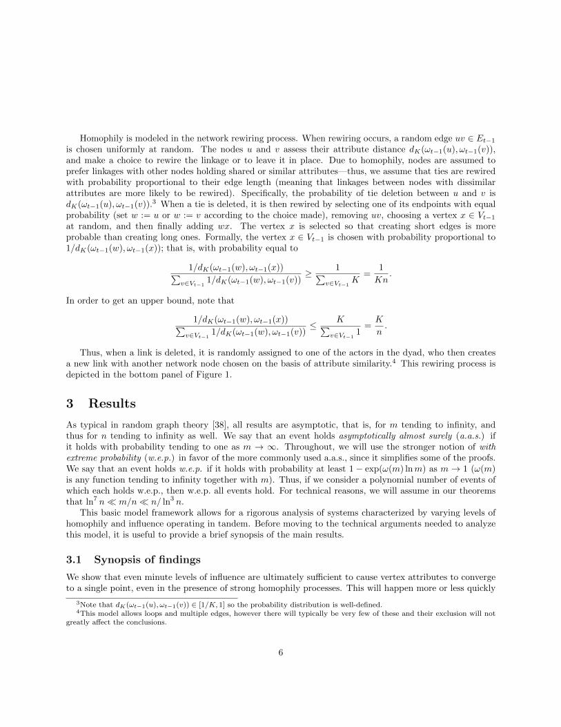
Figure 1: Network evolution process at time t. The figure depicts a schematic of the process for parameters q = 0.5 and K = 8. Nodal attributes arerepresented in the horizontal position of nodes. At time t, either a single node is selected for influence (probability `) or a single edge is selected for rewiring(probability 1 − `). Under influence, the node selected for influence (A in the figure) is pulled to its local center of mass Mt(A), or the average attributeof all neighbors. The attribute of A then shifts q(Mt(A) − ω(A)), or from ω(A) = 0.5 to ω(A) = 0.604 in this example. Under rewiring, an edge (AD) isselected uniformly at random and is deleted with probability dK (ω(A), ω(D)) = 0.375 (proportional to its edge length). A and D are then chosen with equalprobability to rewire the link. The selected node (A in this case) assesses all possible edge lengths in the network and, under homophily, is more likely tocreate a link with a node having similar attributes than with a dissimilar node.

5

Homophily is modeled in the network rewiring process. When rewiring occurs, a random edge uv ∈ Et−1

is chosen uniformly at random. The nodes u and v assess their attribute distance dK(ωt−1(u), ωt−1(v)),and make a choice to rewire the linkage or to leave it in place. Due to homophily, nodes are assumed toprefer linkages with other nodes holding shared or similar attributes—thus, we assume that ties are rewiredwith probability proportional to their edge length (meaning that linkages between nodes with dissimilarattributes are more likely to be rewired). Specifically, the probability of tie deletion between u and v isdK(ωt−1(u), ωt−1(v)).3 When a tie is deleted, it is then rewired by selecting one of its endpoints with equalprobability (set w := u or w := v according to the choice made), removing uv, choosing a vertex x ∈ Vt−1

at random, and then finally adding wx. The vertex x is selected so that creating short edges is moreprobable than creating long ones. Formally, the vertex x ∈ Vt−1 is chosen with probability proportional to1/dK(ωt−1(w), ωt−1(x)); that is, with probability equal to

1/dK(ωt−1(w), ωt−1(x))∑v∈Vt−1

1/dK(ωt−1(w), ωt−1(v))≥ 1∑

v∈Vt−1K

=1

Kn.

In order to get an upper bound, note that

1/dK(ωt−1(w), ωt−1(x))∑v∈Vt−1

1/dK(ωt−1(w), ωt−1(v))≤ K∑

v∈Vt−11

=K

n.

Thus, when a link is deleted, it is randomly assigned to one of the actors in the dyad, who then createsa new link with another network node chosen on the basis of attribute similarity.4 This rewiring process isdepicted in the bottom panel of Figure 1.

3 Results

As typical in random graph theory [38], all results are asymptotic, that is, for m tending to infinity, andthus for n tending to infinity as well. We say that an event holds asymptotically almost surely (a.a.s.) ifit holds with probability tending to one as m → ∞. Throughout, we will use the stronger notion of withextreme probability (w.e.p.) in favor of the more commonly used a.a.s., since it simplifies some of the proofs.We say that an event holds w.e.p. if it holds with probability at least 1− exp(ω(m) lnm) as m→ 1 (ω(m)is any function tending to infinity together with m). Thus, if we consider a polynomial number of events ofwhich each holds w.e.p., then w.e.p. all events hold. For technical reasons, we will assume in our theoremsthat ln7 n m/n n/ ln3 n.

This basic model framework allows for a rigorous analysis of systems characterized by varying levels ofhomophily and influence operating in tandem. Before moving to the technical arguments needed to analyzethis model, it is useful to provide a brief synopsis of the main results.

3.1 Synopsis of findings

We show that even minute levels of influence are ultimately sufficient to cause vertex attributes to convergeto a single point, even in the presence of strong homophily processes. This will happen more or less quickly

3Note that dK(ωt−1(u), ωt−1(v)) ∈ [1/K, 1] so the probability distribution is well-defined.4This model allows loops and multiple edges, however there will typically be very few of these and their exclusion will not

greatly affect the conclusions.

6

under different scenarios, and in some cases it is possible to predict with greater precision the process bywhich vertex attributes converge.

When the process begins at t = 0, vertex attributes may follow any distribution and the network G0

may take on any initial structure. As the network undergoes subsequent rewirings, eventually each endpointof each link has been rewired at least once—we call this time T . At this point, a sufficient amount ofrandomness has been introduced into the process, and we are able to predict the behavior of the model withhigh probability. We are able to establish an upper bound for T that is of order m logm (see Lemma 1).

After time T , it is useful to split the analysis of the network evolution process into two cases: first, wherenetwork rewirings do not take into account vertex attributes (the “zero homophily” case where K = 1, inwhich all edges are assigned the same distance, and thus independently of the underlying network, a rewiringis chosen uniformly at random), and second, where vertices cut and form ties on the basis of attributesimilarity (the “homophily” case where K ≥ 2; in which a rewiring is more likely to appear between closevertices). Analyzing the zero homophily case is useful as results from this more specific model may be appliedto the analysis of models with either weak or strong homophily processes (K ≥ 2 with K small or large,respectively).

In the zero homophily case, we can predict the specific process by which attributes converge. After timeT , the local center of mass of each vertex is equal to the global center of mass in expectation, and in factwith high probability all local centers of mass are well concentrated around the global center of mass (seeLemma 2(i)). This means that the attributes of any given node’s neighbor are similar to a random sample ofvertex attributes drawn from the entire network. At this point in time, network structures will be similar tobinomial random graphs. While vertex attributes have not necessarily converged at this point, these resultsimply that by time T any segregation seen in initial network conditions will have been destroyed by theinfluence processes without homophily supporting cross-group partitions. After at most T = Θ(`−1n lnn)more steps, all vertex attributes have then finally converged to the global center of mass. This result is givenin Theorem 3.

In the homophily case, Lemma 2(ii) demonstrates that by time T , the local centers of mass are beingpushed away from their boundaries towards the global center of mass. This means that the local centers ofmass will typically be some fraction of the distance between that vertex’s attribute and the global center ofmass. We can specify an upper bound on this distance, which increases as the tendency towards homophilyincreases (that is, as K gets larger). Networks at this point exhibit network segregation as studied in [32]in that linkages in the network tend to be “short,” that is, connecting vertices with similar attributes. Ifvertex attributes ωt(v) maintain a multi-modal distribution at this point, then a clear community structurewill emerge.

In both cases (that is, for any value of K), vertex attributes begin to converge after time T up to sometime T + T . In the absence of homophily, all vertex attributes at time T + T will be very close (withino(ln−2 n) = o(1)) of the global center of mass (see Theorem 3).5 The bigger n is, the closer all vertexattributes will be. This is because, for large n, the concentration results are stronger and the behavior of thewhole network is even more predictable. An upper bound for T + T is identified in Theorem 3. Moreover, weare able to predict precisely the process by which this convergence to the global center of mass takes place,in terms of how the average distance between each individual vertex and the global center of mass changesover time. The behavior of this random variable is predicted using the differential equation method and isspecified in Theorem 12.

5We use the following standard asymptotic notation: f(n) = o(g(n)), if limn→∞ f(n)/g(n) = 0, and f(n) = O(g(n)) if thereexists some n0 so that for all n ≥ n0, f(n) ≤ Cg(n) for some absolute constant C > 0. Similarly, if f(n) = O(g(n)), theng(n) = Ω(f(n)), and if both f(n) = O(g(n)) and g(n) = O(f(n)) hold, then f(n) = Θ(g(n)).

7

In the presence of homophily, we determine an upper bound for the time when all vertex attributesare within 1/K of each other (see Theorem 5). At this point, the attributes of nodes are within a smallenough interval that the distinctions between vertex attributes begin to disappear, meaning that homophilyno longer exercises a noticeable influence on the network structure. From this point on, findings from theK = 1 case may be applied to show that, after another T time steps, the local centers of mass are wellconcentrated around the global center of mass as shown in Lemma 2(i).

The following sections analyze the model in more depth by asking (and answering!) a series of questionsabout the model’s behavior with some constraints placed on parameters. Ultimately, these answers allowus to make precise predictions about how the model behaves without any parameter constraints. Muchof the mathematical logic underlying these results is contained in the proofs, which are included in theSupplemental Information for interested readers.

3.2 How long does it take to rewire each edge endpoint at least once?

Each time a rewiring occurs, an edge is selected uniformly at random (that is, a given edge is selected withprobability 1/m), and then one of the endpoints of this edge is selected uniformly at random (that is, withprobability 1/2). So in each rewiring step, one of the 2m edge endpoints is selected uniformly at randomand is associated with a random vertex. Although vertices that are more similar to the selected endpointhave a higher probability of being chosen, a given vertex is always selected with probability at least 1/(Kn).These steps occur independently of the history of the process.

Based on the following lemma, we know that the time at which each edge endpoint has been rewired atleast once is no later than T , which is of order m lnm. A proof of Lemma 1 is provided in the SupplementalInformation.

Lemma 1. Consider the evolutionary process P(G0, ω0, `, q, r,K) = (Gt, ωt)∞t=0. Let ω(m) be any function

that tends to infinity as m → ∞, and let T be the first time every edge has both endpoints rewired at leastonce. Then, a.a.s.

T ≤ 2Km

1− `(lnm+ ω(m)) = Θ(m lnm). (1)

It should be noted that this upper bound is a function of both K and `. This is because, in additionto linkages being rewired, vertex attributes are also being updated as a result of the influence process. Ifthe only process occurring were the rewiring of links, then from the well-known coupon collector problem itwould be sufficient to wait (1 + o(1))2m logm time steps to rewire all 2m edge endpoints.6 But since sometime steps are used for influence rather than rewiring, it is necessary to wait (1 + o(1))(2m/(1 − `)) logmrounds to ensure enough endpoints are rewired. Finally, since edge endpoints are not selected uniformly atrandom (i.e., endpoints associated with long edges have a higher chance of being selected), it is necessary towait even slightly longer (a multiplicative factor of K is sufficient) to make sure that the endpoints of shortedges are rewired as well.

6Let c ∈ R. From the coupon collector problem, it follows that after 2m(ln(2m) + c) rewirings, with probability tending to

e−e−c, every endpoint is rewired at least once. From this it follows that if c→∞, then after 2m(ln(2m) + c) rewirings, a.a.s.

every endpoint is rewired at least once.

8

3.3 Where are local centers of mass relative to the global center of mass?

After the rewiring of every edge endpoint at time T , we can begin to estimate the distance between theglobal center of mass at time t (Mt) and the average attribute of vertex v’s neighbors (v’s local center ofmass, denoted Mt(v)).

Suppose first that K = 1. In this situation, attributes’ differences are irrelevant and edges are rewiredwithout any tendency towards homophily; that is, regardless of whether the selected edge is long (connectingvertices with very different attributes) or short (connecting vertices with very similar attributes). The randomgraph at time T is relatively easy to study. In particular, for a given edge e ∈ E0 from the initial networkG0, t ≥ T , and any two vertices x and y, the probability that e connects x and y at time t is 2/n2. Indeed,with probability 1/n2 the first endpoint was associated with x and the second one with y, at the last timethey were rewired. The same property holds when x is swapped with y. It follows that

P(xy ∈ Et) = 1−(

1− 2

n2

)m

= 1− exp

(−2m

n2+O

(mn4

))=

2m

n2+O

(m2

n4

)=

2m

n2

(1 +O

(mn2

))= (1 + o(ln−3 n))

2m

n2, (2)

provided that m = o(n2/ ln3 n).In this situation, the expected degree of vertices in the network is (1 + o(1))2m/n, and networks exhibit

properties similar to those observed in binomial random graphs G(n, p) with p = 2m/n2. In particular, thelocal centers of mass will be very close to the global one, provided that the network is dense enough to ensurethat a given vertex’s neighbors are representative of the entire set of network nodes.

Suppose now that K ≥ 2. In this case, network rewiring is driven by some degree of homophily where longedges (connecting dissimilar vertices) are terminated with higher probability than short edges, and whereshort edges are formed with higher probability than long edges. This process tends to generate segregated,“attribute-close” networks where most edges are short, connecting vertices with similar or shared attributes;see [32] for more details. Therefore, it is expected that the local center of mass of a vertex v lies between vand the global center of mass.

Indeed, we are able to specify more precisely the distance between the local centers of mass and the globalcenter of mass, in both the K = 1 and K ≥ 2 cases. Since each dimension may be treated independently,we assume without loss of generality that r = 1. These distances are specified in Lemma 2.

Lemma 2. Consider the social process P(G0, ω0, `, q, 1,K) = (Gt, ωt)∞t=0. Suppose that d = 2m/n is such

that ln7 n d = o(n/ ln3 n). Let C > 0. Then, w.e.p. for every T ≤ t ≤ nC and every v ∈ Vt, the followingholds

(i) If K = 1, thenMt(v) = (1 + o(ln−3 n))Mt.

(ii) If K ≥ 2, thenMt(v) ≥ (1 + o(1))K−6Mt + o(ln−5 n)

andMt(v) ≤ 1− (1 + o(1))K−6(1−Mt) + o(ln−5 n).

9

At this point it is possible to have local centers of mass that are outliers, in the sense that vertices arecloser to the global center of mass than their neighbors. In this case, local centers of mass can be pulled awayfrom the global center because of the influence of their neighbors, but this does not substantially affect theglobal dynamics. However, once all vertex attributes are trapped in a particular interval, they will alwaysremain within that interval. This observation—which we elaborate on in the following sections—tells us thatlocal centers of mass that are outliers and close to the boundaries will tend to be pushed towards the globalcenter of mass, causing the length of this interval in which all vertex attributes are “trapped” to shrink overtime.

3.4 How quickly do vertex attributes converge in the absence of homophily?

We now consider the model’s behavior in the absence of homophily—that is, when K = 1 and edge rewiringsare independent of vertex attributes. These results may then be applied with some modifications to theunconstrained case where K ≥ 1. For the sake of brevity, we state the final result for the K = 1 case here asTheorem 3. The Supplemental Information contains a formal proof of Theorem 3 as well as a full explanationof the logic of how this result is obtained through the analysis of a series of more simple models.

Theorem 3. Consider the evolutionary process P(G0, ω0, `, q, r, 1) = (Gt, ωt)∞t=0. Suppose that d = 2m/n is

such that ln7 n d = o(n/ ln3 n) and ` ≥ n−C for some C ≥ 1, and recall the definition of T in (1). Then,a.a.s.

‖ωT+T (v)−MT ‖ = o(ln−2 n) = o(1)

for every v ∈ VT+T , where T = `−1(2 + ε)n lnn for some ε > 0.

Note that a.a.s.T + T = Θ(m lnm) + Θ(`−1n lnn) = O(nC+1 lnn).

Theorem 3 says that, at time T + T and for K = 1, the distance between each vertex’s attributeand the global center of mass is o(ln−2 n); in words, the bigger n, the closer all vertex attributes are. Theintuition behind this is that as the value of n grows, the process becomes more predictable (since the variancedecreases by the law of large numbers). More precisely, all vertex attributes are in some interval (a, b) oflength o(ln−2 n) and, once all attributes are in this interval, they will always remain there.

3.5 What is the process by which attributes converge in the absence of ho-mophily?

Above, we demonstrated that vertex attributes will converge when K = 1. Additionally, it is possible topredict the convergence process between time T and T + T . This is done using the differential equation(DE) method [58], which allows us to show that a.a.s. the average distance between vertex attributes andthe global center of mass at a given time period decreases in a predictable way. An introduction to the DEmethod is provided in the Supplemental Information.

Formally, let

Wt =∑v∈Vt

|ωt(v)−Mt|.

The random variable Wt represents the overall deviations between the global center of mass and allindividual local centers of mass at time t. Corollary 4 specifies how this random variable behaves over time.

10

Corollary 4. Consider the evolutionary process P(G0, ω0, `, q, r, 1) = (Gt, ωt)∞t=0. Suppose that d = 2m/n

is such that ln7 n d = o(n/ ln3 n) and ` ≥ n−C for some C ≥ 1. Then, a.a.s.

Wt = (1 + o(1))WT exp

(−q`(t− T )

n

)for every t such that T ≤ t ≤ T + tf , where T is defined in (1) and

tf =n

q`

(ln lnn− ln

(n

WT

)).

This result is a corollary to Theorem 12, which is explained in further detail (and proven) in the Supple-mental Information.

3.6 Model behavior with homophily, K ≥ 2

In a homophilous network, there is a bias for the termination of long edges and the creation of short edges.Suppose that all vertex attributes lie in the interval [a, b] (as usual, we may treat all dimensions independentlyand so it is enough to focus on one dimension). It follows from Lemma 2(ii) that when vertex v is selectedfor influence at time t ≥ T , it is moved away from at least one border of the attribute space (i.e., the valuea or b). While the exact updated attribute of each vertex selected for influence cannot be predicted, it isknown that the global center of mass is positioned far enough from one end of the interval such that allvertices selected for influence are pushed away from that end. Unfortunately, the global center of mass mightbe shifting during this process, and it is likely impossible to precisely predict how the global center of massmoves over time. This is in contrast to the result for the K = 1 case (see Theorem 3), which says that theglobal center of mass does not drift substantially between times T and T + T .

Fortunately, it is possible to show that after at most 3`−1n lnn steps, w.e.p. the maximum distance be-tween any pair of nodes shrinks (in each dimension) by a multiplicative factor of at least ε := q(13K12n lnn)−1.That is, if the distance is D at some time t, at time t + 3`−1n lnn it is w.e.p. at most D(1 − ε). This isan upper bound only, and it is expected that the convergence process is in fact more rapid. A proof ofTheorem 5 is provided in the Supplemental Information:

Theorem 5. Consider the evolutionary process P(G0, ω0, `, q, r,K) = (Gt, ωt)∞t=0. Suppose that d = 2m/n

is such that ln7 n d = o(n/ ln3 n) and ` ≥ n−C for some C ≥ 1. Then, a.a.s. for every pair u, v ∈ Vt wehave

|ωt(u)− ωt(v)| ≤√r(

1− q

13K12n lnn

)b`(t−T )/(3n lnn)c

≤√r exp

(−qb`(t− T )/(3n lnn)c

13K12n lnn

)for every t such that T ≤ t = O(`−1n2 ln2 n) (the random variable T is defined in (1)). In particular, ift = cq−1`−1n2 ln2 n for some constant c > 0, then a.a.s. for every pair u, v ∈ Vt we have

|ωt(u)− ωt(v)| ≤ (1 + o(1))√r exp

(− c

39K12

).

11

This result implies that at some time

T ≤(

1

2ln r + lnK + 1

)39K12(q−1`−1n2 ln2 n) = O(`−1n2 ln2 n)

a.a.s. all vertex attributes are within distance 1/K of each other. At this point, the attributes of nodes arewithin a small enough interval that the distinctions between vertex attributes begin to disappear, meaningthat homophily no longer exercises a noticeable influence on the network structure. From this point on,findings from the K = 1 case may be applied to show that, after another T time steps, the local centers ofmass are well concentrated around the global center of mass as shown in Lemma 2(i). With this result inhand, the behavior of the process can be predicted quite easily, and a.a.s. all the vertex attributes convergeto a single point.

Corollary 6. Consider the evolutionary process P(G0, ω0, `, q, r,K) = (Gt, ωt)∞t=0. Suppose that d = 2m/n

is such that ln7 n d = o(n/ ln3 n) and ` ≥ n−C for some C ≥ 1. Let T be the first time all pairs of verticesare within distance 1/K (or T =∞ if this never happens). Then, a.a.s.

T ≤(

1

2ln r + lnK + 1

)39K12(q−1`−1n2 ln2 n) = O(`−1n2 ln2 n)

Moreover,

Wt = (1 + o(1))WT+T exp

(−q`(t− T − T )

n

)for every t such that T + T ≤ t ≤ T + T + tf , where T is defined in (1) and

tf =n

q`

(ln lnn− ln

(n

WT+T

)).

In particular, at time T + T + tf = O(`−1n2 ln2 n) the average distance between vertices is o(1).

4 Examining dynamics through computational simulation

This analysis shows that, for all network structures, very small amounts of influence will lead to a convergencein attributes over time even when homophily (a polarizing force) is very strong. Thus, in theory, even smallamounts of influence are sufficient to overcome even strong patterns of network segregation. The speedof convergence in attributes will of course depend on the relative strength of the homophily and influenceprocesses. The preceding results allow us to predict with more precision the behavior of the system overtime, in terms of how quickly the local centers of mass converge to the global center of mass for a givennetwork. These dynamics are illustrated in Figure 2, which plots the maximum distance between local andglobal centers of mass over time, for 1) varying strengths of influence for a given level of homophily (leftpanel), and 2) varying levels of homophily for a given influence parameter (right panel).

The mathematical model developed here allows for a strong, generalized prediction about the behaviorof networked systems over time. At the same time, the methods used here require limiting our attentionto relatively simple network evolution processes, meaning that we face a fundamental trade-off between

12

Figure 2: Upper bounds on attribute convergence speeds for varying levels of influence and homophily

model complexity and strength of predictions. Computational simulations are one way to introduce morecomplexity into these models, and also illustrate the evolutionary dynamics discussed in this paper. Thus,to complement the main mathematical model, we conducted a series of computational simulations of theinfluence and network rewiring process in small, random networks.7

4.1 Computational model setup

Our computational simulations begin with small, undirected random networks on 30 vertices and 44 edges(yielding a fixed network density of about 0.1). At initialization agents are assigned, uniformly and atrandom, an attribute value of 0 or 1. Links are then assigned with probability proportional to attributesimilarity, so that initial networks exhibit high degrees of segregation and community structure (see, forexample, the top panel of Figure 4). By starting with highly segregated initial network structures, we createconditions that are most favorable for the maintenance of network segregation over time.

With the initial networks in place, at each time step the system undergoes an influence process (whererandomly selected vertices update their attributes based on network position), followed by an edge rewiringprocess (where randomly selected edges are deleted and reallocated to non-adjacent vertices).8 When avertex i is selected for influence, it moves a fraction of the distance between its own attribute and i’s localcenter of mass (i.e., the average attribute of vertex i’s neighbors). This fraction is governed by a modelparameter q ∈ [0, 1] as defined above.

Edge rewiring, on the other hand, progresses in a slightly different manner from the mathematical modelpresented in this paper. When an edge is selected for rewiring, it is randomly rewired by choosing a pair of

7Agent-based models were programmed in R [54]. Visualizations presented here made use of the R sna package [9].8At each time step, 3 vertices are selected uniformly at random for influence and 9 edges are selected uniformly at random

for rewiring. Among the selected vertices and edges, the influence and rewiring processes occur simultaneously. This setup waschosen to speed computation times.

13

non-adjacent vertices with probability proportional to the attractiveness of that pair. In order to account formore drivers of network formation, attractiveness of a potential link between two nodes i and j is allowed tobe a function of three factors, including the similarity of nodal attributes (representing the tendency towardshomophily), the number of paths of length 2 between i and j (representing the tendency towards transitivity,or so called triadic closure), and the degree of nodes i and j (representing the tendency towards forminglinkages with high-degree actors, as in a preferential attachment model). In general, the attractiveness of alink between non-adjacent vertices i to j is assumed to be

ai→j =1

dK(i, j)+ pclosureT (i, j) + pdegreed(j),

whereK is a simulation parameter representing the strength of the homophily effect, dK(i, j) is the discretizeddistance between vertices i and j (as described earlier), pclosure is a simulation parameter representing thestrength of triadic closure, T (i, j) is the number of paths of length 2 between vertices i and j, pdegree is

a simulation parameter representing the strength of vertex degree, and d(j) is the degree of j, that is, thenumber of vertices adjacent to j.

Thus, the attractiveness of two non-adjacent vertices depends on their distance, the degree of the incomingvertex, and the number of common neighbors of i and j. When an edge is selected for rewiring, theattractiveness scores of non-adjacent vertices are calculated. The resultant set of attractiveness scores isthen converted into a probability distribution from which a particular dyad is selected—the edge selectedfor rewiring is then relocated to this randomly-chosen dyad.

The attractiveness of pairs of vertices based on these effects is illustrated in Figure 3. From the perspectiveof a particular vertex (labeled Ego in Figure 3), different potential linkages (non-adjacent vertices in the farleft panel) have varying levels of attractiveness. Potential links are depicted as dashed red lines, and theirattractiveness depends on the three simulation parameters triadic closure, degree, and homophily (K).9 Withhigher triadic closure parameters, Ego will tend to view linkages that create triangles as more attractive, andtherefore Ego will want to form a link with A in this schematic. With higher degree parameters, Ego willtend to view linkages with high degree vertices (e.g., vertex B) as more attractive. With higher homophilyparameters, Ego will tend to view links as more attractive when the linkage reduces the difference betweenEgo’s attribute and Ego’s local center of mass (e.g., a link with vertex C).

4.2 Simulation results

Figure 4 displays one typical simulation run. On the left side of the figure are depictions of the networkrealized at each time step. In this diagram, the color of vertices indicate their starting attribute (0 or 1),and vertex sizes are proportional to the vertex’s local center of mass and the network’s global center of mass.The right side of the figure displays the distribution of the local centers of mass of each vertex, relative to theglobal center of mass (the global center of mass is indicated by the vertical reference line in the distributionplot). In this particular example, the local centers of mass collapse around the global center of mass after 65time steps. This is also seen in the network diagrams, which show the decay of segregation around sharedattributes early in the process to a well-mixed network where linkages are independent of starting attributes(node color) in the final time step.

Approximately 1,800 simulations were run with three model parameters—homophily, transitivity, anddegree— assigned uniformly at random from [0, 100] and q assigned uniformly at random from [0.15, 1] at each

9The homophily parameter is analogous to the parameter K in the main mathematical model.

14

Figure 3: How simulation parameters change the relative attractiveness of pairs of vertices

simulation run. Consistent with our findings reported earlier, these simulations show that in all cases—evenwhen additional network evolution dynamics are taken into account—vertex attributes always converge suchthat local centers of mass eventually collapse to the global center of mass. These dynamics are summarizedin Figure 5. This figure plots the distribution of maximum distance between all local centers of mass andthe global center of mass, for each simulation, and at different stages of the process. In order to visualize allsimulations on a common scale, the distributions are represented at the initial time step in the far left, andsubsequent distributions are for one-tenth of the final time step, two-tenths of the final time step, and so on.In the final time step, the maximum distance between the global and local centers of mass is no more than0.05.

Figure 5 shows a large amount of variation in convergence patterns, however in aggregate we see a cleartrend towards attribute convergence. But while attributes tend towards a single point, it is useful to examinehow variation in the simulation parameters explain the speed of attribute convergence. Figure 6 summarizesthese patterns by fitting an OLS linear regression model with time to convergence as the dependent variable,and simulation parameters as independent variables. Specifically, we model time to convergence as a linearcombination of simulation parameters using the individual simulation run as the unit of analysis:

Y = b0 + b1 · pclosure + b2 · pdegree + b3 ·K + b4 · q + e,

where Y is a simulation’s time to convergence, b0, b1, b2, b3, and b4 are constant coefficients, e is an errorterm, and pclosure, pdegree, K, and q represent (respectively) the model parameters described above: the

tendency towards triadic closure, the tendency to form ties with high-degree actors, homophily, and influence.These results indicate that triadic closure and homophily have complementary effects on convergence

speeds; both are positive, with roughly the same magnitude. This means that homophily and closure bothtend to increase convergence times—that is, network segregation will take longer to disappear when tieformation is driven by homophily and triadic closure. This does make intuitive sense. If a network exhibitssegregation, then triadic closure will tend to amplify the formation of ties among similar vertices becauseneighbors of neighbors will also tend to have similar attributes. On the other hand, introducing triadicclosure does not prevent attributes from converging any more than homophily does.

Seeking out vertices with high degree appears to speed the process of convergence. This also makesintuitive sense, since this is a process that allows ties to be formed independently of attributes. So while

15

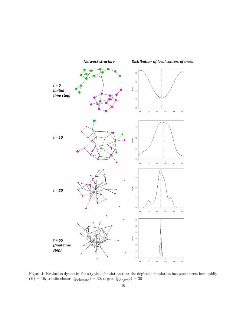
Figure 4: Evolution dynamics for a typical simulation run: the depicted simulation has parameters homophily(K) = 10; triadic closure (pclosure) = 30; degree (pdegree) = 30

16

Figure 5: Aggregate simulation behavior over time

17

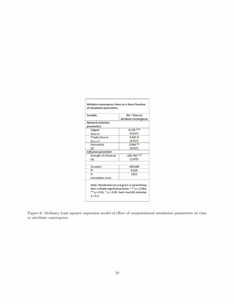
Figure 6: Ordinary least squares regression model of effect of computational simulation parameters on timeto attribute convergence

18

triadic closure will tend to create more short edges in the presence of network segregation, forming linkson the basis of degree has nothing to do with attributes and provides a way for vertices to “escape” fromhomogenous network neighborhoods. The overall effect of degree-seeking is larger than both the homophilyand triadic closure effects, meaning that degree-seeking behavior will tend to decay network segregationmuch faster than homophily or closure can maintain it.

5 Conclusion

This paper shows that influence processes are able to overcome the polarizing effect of homophily in creatingsegregated networks, even when strong forms of homophily are coupled with a relatively weak influenceprocess. We prove mathematically that asymptotically almost surely, the size of the interval containing allvertex attributes tends to zero as t approaches infinity. In other words, the distinctions between vertices basedon malleable attributes eventually disappear, which in turn prevents homophily from influencing emergentnetwork structures.

Network segregation and related concepts, such as community structure, are well-studied phenomenain self-organizing networks. But why does network segregation emerge, and how is it maintained overtime? Developing better models of these dynamics is important because they can suggest ways to managethe problems that arise from segregated networks—such as conflict or mistrust between social groups, ordifficulties in searching for diverse sources of information.

While small amounts of homophily are sufficient to produce segregated networks when attributes arefixed, once malleability of attributes is introduced it becomes difficult to model the persistence of networksegregation over time. We show mathematically that an important class of models, those where attributesmove (potentially very slowly) towards one another, cannot maintain network segregation indefinitely. Whileour definition of influence represents one of many possibilities of how attributes change dynamically, theseresults are more powerful than those inferred from simulations that can only investigate a finite numberof possible scenarios (and yet, the results are also supported by computational simulations that includemore complex network evolution processes). With this research, we hope to provide a baseline for moreinvestigations into the micro-level processes that generate and maintain the network segregation that isobserved empirically across a wide range of self-organizing networks.

References

[1] Aiello, W., Bonato, A., Cooper, C., Janssen, J., and Pra lat, P. (2009) A spatial web graph model withlocal influence regions, Internet Mathematics 5, pp. 175–196.

[2] Aral, S., Muchnik, L. and Sundararajan, A. (2013) Engineering Social Contagions: Optimal NetworkSeeding in the Presence of Homophily. Network Science 1, 125153.

[3] Banerjee, A., Chandrasekhar, A. G., Duflo, E., and Jackson, M. O. (2013). The Diffusion of Microfinance.Science, 341(6144), 12364981236498.

[4] Barabasi, A.-L. and Albert, R. (1999) Emergence of Scaling in Random Networks, Science, vol. 286, no.5439, pp. 509–512.

[5] Boardman, J. D., Domingue, B. W., and Fletcher, J. M. (2012). How Social and Genetic Factors PredictFriendship Networks. Proceedings of the National Academy of Sciences, 109(43), 1737717381.

19

[6] Boucher, V. (2015). Structural Homophily. International Economic Review, 56(1), 235264.

[7] Bramoulle, Y., Currarini, S., Jackson, M. O., Pin, P., and Rogers, B. W. (2012). Homophily and Long-Run Integration in Social Networks. Journal of Economic Theory, 147(5), 17541786.

[8] Burt, R. S. (2004) Structural Holes and Good Ideas. Am J Sociol 110, pp. 349–399.

[9] Butts, C. T. (2012) sna: Tools for Social Network Analysis. R package version 2.2-0. http://CRAN.R-project.org/package=sna

[10] Centola, D. (2011). An Experimental Study of Homophily in the Adoption of Health Behavior. Science,334(6060), 12691272.

[11] Centola, D., Gonzalez-Avella, J. C., Eguiluz, V. M., and San Miguel, M. (2007). Homophily, CulturalDrift, and the Co-Evolution of Cultural Groups. Journal of Conflict Resolution, 51(6), 905929.

[12] Cooper, C., Frieze, A., and Pra lat, P. (2014) Some typical properties of the Spatial Preferred Attachmentmodel. Internet Mathematics 10, pp. 27–47.

[13] Cooper, C., Pra lat, P. (2011) Scale-free graphs of increasing degree. Random Structures and Algorithms38, pp. 396–421.

[14] Currarini, S., Jackson, M. O., and Pin, P. (2009). An Economic Model of Friendship: Homophily,Minorities and Segregation. Econometrica, 77(4), 10031045. http://doi.org/10.2139/ssrn.1021650

[15] Currarini, S., Jackson, M. O., and Pin, P. (2010). Identifying the Roles of Race-Based Choice andChance in High School Friendship Network Formation. Proceedings of the National Academy of Sciences,107(11), 48574861.

[16] Danchin, E., Giraldeau, L.-A., Valone, T. J. and Wagner, R. H. (2004) Public Information: From NosyNeighbors to Cultural Evolution. Science 305, pp. 487–491.

[17] Dandekar, P., Goel, A., and Lee, D. T. (2013). Biased Assimilation, Homophily, and the Dynamics ofPolarization. Proceedings of the National Academy of Sciences, 110(15), 57915796.

[18] DeGroot, M. H. (1974) Reaching a Consensus. Journal of the American Statistical Association 69,pp. 118–121.

[19] Dietz, T. (2013) Bringing Values and Deliberation to Science Communication. Proceedings of the Na-tional Academy of Sciences 110, pp. 14081–14087.

[20] D’Souza, R. M., Borgs, C., Chayes, J. T., Berger, N. and Kleinberg, R. D. (2007) Emergence of Tem-pered Preferential Attachment from Optimization. Proceedings of the National Academy of Sciences 104,pp. 6112–6117.

[21] Durrett, R. et al. (2012) Graph fission in an evolving voter model. Proceedings of the National Academyof Sciences 109, pp. 3682–3687.

[22] Freeman, L. C. (1978) Segregation in Social Networks. Sociological Methods & Research 6, 411429.

20

[23] Friedkin, N. E., and Johnsen, E. C. (2011) Social Influence Network Theory: A Sociological Examinationof Small Group Dynamics, Cambridge University Press.

[24] Gerber, E. R., Henry, A. D., and Lubell, M. (2013). Political Homophily and Collaboration in RegionalPlanning Networks. American Journal of Political Science, 57(3), 598610.

[25] Girard, Y., Hett, F., and Schunk, D. (2015). How Individual Characteristics Shape the Structure ofSocial Networks. Journal of Economic Behavior & Organization, 115, 197216.

[26] Girvan, M. and Newman, M.E.J. (2002) Community Structure in Social and Biological Networks. Pro-ceedings of the National Academy of Sciences 99, pp. 7821–7826.

[27] Golub, B., and Jackson, M. O. (2012). Does Homophily Predict Consensus Times? Testing a Model ofNetwork Structure via a Dynamic Process. Review of Network Economics, 11(3).

[28] Granovetter, M. S. (1973) The Strength of Weak Ties. The American Journal of Sociology 78, pp. 1360–1380.

[29] Harris, K. M., Halpern, C. T., Whitsel, E., Hussey, J., Tabor, J., Entzel, P., and Udry, J. R. (2009).The National Longitudinal Study of Adolescent to Adult Health: Research Design. Retrieved fromhttp://www.cpc.unc.edu/projects/addhealth/design

[30] Henry, A. D. (2009) The Challenge of Learning for Sustainability: A Prolegomenon to Theory. HumanEcology Review 16, pp. 131–140.

[31] Henry, A. D. (2011). Ideology, Power, and the Structure of Policy Networks. Policy Studies Journal,39(3), 361383.

[32] Henry, A. D., Pra lat, P. and Zhang, C.-Q. (2011) Emergence of Segregation in Evolving Social Networks.Proceedings of the National Academy of Sciences 108, pp. 8605–8610.

[33] Henry, A. D., Lubell, M., and McCoy, M. (2011). Belief Systems and Social Capital as Drivers of PolicyNetwork Structure: The Case of California Regional Planning. Journal of Public Administration Researchand Theory, 21(3), 419 444.

[34] Henry, A. D., and Pra lat, P. (2013). Discovery of Nodal Attributes through a Rank-Based Model ofNetwork Structure. Internet Mathematics, 9(1), 3357.

[35] Hong, L. and Page, S. E. (2004) Groups of Diverse Problem Solvers Can Outperform Groups of High-Ability Problem Solvers. Proceedings of the National Academy of Sciences 101, pp. 16385–16389.

[36] Jackson, M. O. (2014). Networks in the Understanding of Economic Behaviors. Journal of EconomicPerspectives, 28(4), 322.

[37] Jackson, M. O. and Lopez-Pintado, D. (2013) Diffusion and Contagion in Networks with HeterogeneousAgents and Homophily. Network Science 1, 4967.

[38] Janson, S., Luczak, T., and Rucinski, A. (2000) Random Graphs. Wiley, New York.

[39] Kleinbaum, A. M., Stuart, T. E., and Tushman, M. L. (2013). Discretion Within Constraint: Homophilyand Structure in a Formal Organization. Organization Science, 24(5), 13161336.

21

[40] Kossinets, G., and Watts, D. J. (2009). Origins of Homophily in an Evolving Social Network. AmericanJournal of Sociology, 115(2), 405450.

[41] Krause, A.E., Frank, K. A., Mason, D. M., Ulanowicz, R. E. and Taylor, W. W. (2003) CompartmentsRevealed in Food-Web Structure. Nature 426, 282285.

[42] Kumpula, J., Onnela, J.-P., Saramaki, J., Kaski, K. and Kertesz, J. (2007) Emergence of Communitiesin Weighted Networks. Physical Review Letters 99.

[43] Lambiotte, R., Ausloos, M. and Holyst, J. (2007) Majority Model on a Network with Communities.Physical Review E 75.

[44] Lazer, D. (2001) The Co-Evolution of Individual and Network. The J. of Math. Sociology 25, pp. 69–108.

[45] Lewis, K., Gonzalez, M., and Kaufman, J. (2012). Social Selection and Peer Influence in an OnlineSocial Network. Proceedings of the National Academy of Sciences, 109(1), 6872.

[46] McPherson, M., Smith-Lovin, L. and Cook, J. M. (2001) Birds of a Feather: Homophily in SocialNetworks. Annual Review of Sociology 27, pp. 415–444.

[47] Newman, M. E. J. (2003) The Structure and Function of Complex Networks. SIAM Review 45, pp. 167–256.

[48] Newman, M. E. J. (2006) Modularity and Community Structure in Networks. Proceedings of the NationalAcademy of Sciences 103, pp. 8577–8582.

[49] Nowak, M. A. (2006) Five Rules for the Evolution of Cooperation. Science 314, pp. 1560–1563.

[50] Palla, G., Barabasi, A.-L. and Vicsek, T. (2007) Quantifying social group evolution. Nature 446, pp. 664–667.

[51] Palla, G., Derenyi, I., Farkas, I. and Vicsek, T. (2005) Uncovering the Overlapping Community Structureof Complex Networks in Nature and Society. Nature 435, pp. 814–818.

[52] Parson, E. A. and Clark, W. C. (2005) in Barriers and Bridges to the Renewal of Ecosystems andInstitutions, pp. 428–460, Columbia University Press.

[53] Porter, M. A., Onnela, J.-P. and Mucha, P. J. (2009) Communities in Networks. Notices of the AmericanMathematical Society 56, pp. 1082–1097.

[54] R Core Team (2012) R: A language and environment for statistical computing. R Foundation for Sta-tistical Computing, Vienna, Austria. ISBN 3-900051-07-0, URL http://www.R-project.org/.

[55] Sabatier, P. E. (2007) Theories of the Policy Process. Westview Press.

[56] Sabatier, P. E. and Jenkins-Smith, H. C. (1993) Policy Change and Learning: An Advocacy CoalitionApproach. Westview Press.

[57] Valente, T. W. (1995) Network Models of the Diffusion of Innovations. Hampton Press.

[58] Wormald, N. (1999) The differential equation method for random graph processes and greedy algorithms.In: Lectures on Approximation and Randomized Algorithms, eds. M. Karonski and H. J. Promel, PWN,Warsaw, pp. 73–155.

22

6 Supplemental Information

6.1 Introduction to the Differential Equation method

The general setting that is used in the DEs method [58] is a sequence of random processes indexed by n(which in our case is the number of objects in any set Vt). The aim is to find properties of the random processin the limit as n → ∞. The conclusion we aim for is that variables defined on a random process are wellconcentrated, which informally means that with high probability they are very close to certain deterministicfunctions. These functions arise as the solution to a system of ordinary first-order differential equations. Oneof the important features of this approach is that the computation of the approximate behavior of processesis clearly separated from the proof that the approximation is correct.

To show that the random variables in a process usually approximate the solution of differential equations,we need to use large deviation inequalities. These inequalities are often used to give an upper bound on theprobability that a random variable deviates very far from its expected value. In a typical situation with arandom process, the aim is to show that the random variable Yt of interest is sharply concentrated. In fact,

Yt − Y0 =

t∑i=1

(Yi − Yi−1).

If the differences Yi − Yi−1 are independent, then the Chernoff bound is very useful, see for example Theo-rem 2.8 [38].

Theorem 7. Let X be a random variable that can be expressed as a sum X =∑n

i=1Xi of independentrandom indicator variables where Xi ∈ Bernoulli(pi) with (possibly) different pi = P(Xi = 1) = E[Xi]. Thenthe following holds for t ≥ 0:

P(X ≥ E[X] + t) ≤ exp

(− t2

2(E[X] + t/3)

),

P(X ≤ E[X]− t) ≤ exp

(− t2

2E[X]

).

In particular, if ε ≤ 3/2, then

P(|X − E[X]| ≥ εE[X]) ≤ 2 exp

(−ε

2E[X]

3

). (3)

Strong concentration results of a sequence of not necessarily independent random variables can also beobtained if two consecutive random variables do not differ by too much and have the same (or similar)expectations. This is formalized using the concept of martingales, introduced next.

Definition 8. A martingale is a sequence X0, X1, . . . of random variables defined on the random processsuch that

E[Xn+1 | X0, X1, . . . , Xn] = Xn.

In most applications, the martingale satisfies the property that

E[Xn+1 | X0, X1, . . . , Xn] = E[Xn+1 | Xn] = Xn.

23

As a simple example, consider the following “random walk.” Toss a coin n times. Let Sn be the differencebetween the number of heads and the number of tails after n tosses. Sn is a martingale. Indeed,

E[Sn+1 | Sn] = Sn +1

2· 1 +

1

2· (−1) = Sn.

Clearly, the expected value of Sn is zero. Thus, it is natural to expect that Sn stays relatively closeto zero. The following well-known Hoeffding-Azuma inequality serves as a tool to investigate this, see forexample Theorem 2.25 [38].

Lemma 9. Let X0, X1, . . . be a martingale. Suppose that there exist constants ck > 0 such that

|Xk −Xk−1| ≤ ck

for each k ≤ n. Then, for every t > 0,

P(Xn ≥ E[Xn] + t) ≤ exp

(− t2

2∑n

k=1 c2k

),

P(Xn ≤ E[Xn]− t) ≤ exp

(− t2

2∑n

k=1 c2k

).

This is often applied with t growing much faster than√n and the ck all small non-zero integers. In the

martingale discussed above ck = 1 for all k. Hence,

P(|Sn| ≥ α√n) ≤ 2 exp

((α√n)2

2n

)= 2 exp

(α2/2

),

which is arbitrarily small for α large enough.Finally, let us mention that the Hoeffding-Azuma inequality can be generalized in many ways: an anal-

ogous inequality holds for supermartingales (E[Xn+1|Xn] ≤ Xn) as well as submartingales (E[Xn+1|Xn] ≥Xn). Our proofs use the supermartingale method as described in Corollary 4.1 of [58]. We will use thefollowing lemma, that follows from the generalized Hoeffding-Azuma inequality.

Lemma 10. Let G0, G1, . . . , GL be a random process and Xt a random variable determined by G0, G1, . . . , Gt,0 ≤ t ≤ L. Suppose that for some real β and γ,

E(Xt −Xt−1 | G0, G1, . . . , Gt−1) < β

and

|Xt −Xt−1 − β| ≤ γ

for 1 ≤ t ≤ L. Then for all ε > 0,

P(For some t with 0 ≤ t ≤ L : Xt −X0 ≥ tβ + ε

)≤ exp

(− ε2

2Lγ2

).

24

6.2 The role of the parameter `

The parameter ` controls the relative speed of the influence and rewiring process in the network. Notethat setting ` = 0.5 (such that influence and rewiring occurs with equal probability at each time step) willcause attribute updating (via influence) to occur for a given node far more frequently than link rewiring (viahomophily) for a given edge. This is a result of most networks having far more links than nodes.

To allow for the direct specification of the relative speed of rewiring versus influence, let ` = `(n,m) tobe a function of the number of nodes and edges, and let ` tend to zero as n→∞. Let `0 be such that

`01− `0

=n

m,

and consider the evolutionary process run with parameter `0. Note that when t = cn/`0 steps are performed(for some c ∈ (0,∞)), we expect `0t = cn influence steps and so an 1− e−c fraction of vertices should be hit.On the other hand, after t steps, the number of rewirings is expected to be (1− `0)t = cn(1− `0)/`0 = cmand so we expect to hit an 1 − e−c fraction of edges as well. Note also that `0 = (1 + o(1))n/m = o(1),provided that n = o(m) which is usually the case. For n = cm for some c ∈ (0, 1) we have `0 = c/(1+ c) > 0.There are three possible behaviors that might be desired for different scenarios:

• the two processes are of the same speed: ` = `0,

• there are more influence steps than rewiring ones: ` > `0,

• there are more rewiring steps than influence steps: ` < `0.

6.3 Proof of Lemma 1

Lemma 1 specifies the maximum length of time that is required to rewire each edge endpoint at least onetime, and is stated in the main paper. In particular, Lemma 1 says that the time at which each edge endpointhas been rewired at least once is no later than T , which is of order m lnm.

Lemma. Consider the evolutionary process P(G0, ω0, `, q, r,K) = (Gt, ωt)∞t=0. Let ω(m) be any function

that tends to infinity arbitrarily slowly as m→∞, and let T be the first time every edge has both endpointsrewired at least once. Then, a.a.s.

T ≤ 2Km

1− `(lnm+ ω(m)) = Θ(m lnm). (4)

Proof. Define T ∗ = 2Km1−` (lnm+ ω(m)) for some function ω(m) tending to infinity arbitrarily slowly. Fix

a permutation of length 2m of all edge endpoints in the initial network G0. For i ∈ 1, 2, . . . , 2m, let Ai

be the event that the ith endpoint is not rewired after T ∗ steps. Note that at every step of the process, agiven endpoint is rewired with probability at least (1− `)/(2Km). Therefore, independently of the previoussteps, we have that for every i ∈ 1, 2, . . . , 2m, and denoting by ω(m) any function tending to infinity withm arbitrarily slowly,

P(Ai) ≤(

1− 1− `2Km

)T∗

= exp

(− (1− `)T ∗

2Km+O

(T ∗

m2

))= (1 + o(1)) exp (− lnm− ω(m))

= o(m−1).

25

Therefore, the expected number of endpoints not rewired is 2m · o(m−1) = o(1) and so a.a.s. every endpointis rewired at least once by Markov’s inequality. 3

6.4 Proof of Lemma 2

After time T , it is possible to make certain inferences about the distance of local centers of mass from theglobal center of mass. These results are specified in Lemma 2.

Lemma. Consider the social process P(G0, ω0, `, q, 1,K) = (Gt, ωt)∞t=0. Suppose that d = 2m/n is such that

ln7 n d = o(n/ ln3 n). Let C > 0. Then, w.e.p. for every T ≤ t ≤ nC and every v ∈ Vt, the following holds

(i) If K = 1, thenMt(v) = (1 + o(ln−3 n))Mt.

(ii) If K ≥ 2, thenMt(v) ≥ (1 + o(1))K−6Mt + o(ln−5 n)

andMt(v) ≤ 1− (1 + o(1))K−6(1−Mt) + o(ln−5 n).

Proof. As noted above, each dimension may be treated independently. Thus, without loss of generality wemay assume that r = 1 and ωt : Vt → [0, 1]. Fix t ≥ T and v ∈ Vt. Since we consider a polynomial numberof events only, it is enough to show that each of them holds w.e.p.

The proof of part (i) is a simple application of the Chernoff bound. Let

X =∑

u∈Nt(v)

ωt(u) = |Nt(v)|Mt(v);

that is, X is the sum of distances from the beginning of the interval [0, 1] to all the neighbors of v. As wealready noticed, Mt(v) = X/|Nt(v)|, so it remains to estimate the random variable X and the degree of vindependently. Note that, without loss of generality, we may assume that Mt = Mt(n) ≥ 1/2, since there isno difference whether we measure the distance from the beginning of the interval [0, 1] or from the end. Forany fixed value of Mt, it follows from (2) that

E[X] =∑u∈Vt

P(vu ∈ Et)ωt(u)

= (1 + o(ln−3 n))2m

n2

∑u∈Vt

ωt(u)

= (1 + o(ln−3 n))2m

nMt

= (1 + o(ln−3 n))dMt.

Hence, E[X] = Θ(m/n) = Θ(d) ln7 n. It follows from (3), applied with ε = d−3/7 = o(ln−3 n), that w.e.p.X = (1 + o(ln−3 n))E[X]. Finally, using the Chernoff bound one more time to estimate the degree of v, weget that w.e.p. |Nt(v)| = (1 + o(ln−3 n))d and the proof of part (i) is finished.

26

In order to prove part (ii), it is convenient to think about the rewiring process as before (see the discussionright before (2)). Since each endpoint is rewired at least once at a given time t ≥ T , we can fix an endpointof some edge and then focus on the last attempt to rewire this endpoint. With probability at least 1/K(and clearly at most 1) the rewiring is performed and a given vertex is chosen with probability at least1/(Kn) (at most K/n, respectively). This implies that for any endpoint and any vertex x with probabilityat least 1/(K2n) (at most K/n, respectively) this endpoint is associated with x. Note that these boundshold independently of the previous steps already performed. Performing the same calculations as in (2) weget

P(xy ∈ Et) ≥ 1−(

1− 2

K4n2

)m

= (1 + o(ln−3 n))2m

K4n2,

and

P(xy ∈ Et) ≤ 1−(

1− 2K2

n2

)m

= (1 + o(ln−3 n))2K2m

n2.

Since Mt(v) ≥ 0 for every v (deterministically), the statement trivially holds when Mt = o(ln−5 n). Hence,we may assume that Mt = Ω(ln−5 n). Using the notation as in part (i), we have

E[X] ≥ (1 + o(1))2mMt

K4n= (1 + o(1))

dMt

K4 ln2 n.

It follows from (3), applied with ε = ln−1/2 n, that w.e.p. X = (1 + o(1))E[X]. Similarly, we get thatw.e.p. |Nt(v)| ≤ (1 + o(1))K2d and so w.e.p. Mt(v) ≥ (1 + o(1))Mt/K

6. The second statement of part (ii) isanalogous, since there is no difference whether we measure the distance from the beginning of the interval[0, 1] or from the end. The proof of part (ii) is complete. 3

6.5 Explanation and proof of Theorem 3

To prepare for the slightly technical argument that is required to analyze the original model, a few simpleprocesses are investigated first in the absence of homophily—that is, when K = 1 and edge rewiringsare independent of vertex attributes. These results may then be applied with some modifications to theunconstrained case where K ≥ 1.

We begin with a modified influence process (Model α) in which a vertex selected for attribute updating ismoved to the global center of mass instead of the local center of mass. A second model (Model β) investigatesa process in which there is no bias towards short edges (K = 1) and vertex attributes shift rapidly (q = 1)before generalizing the process (Model γ) to a slower version where attributes are more resistant to change(q < 1).

Since the first steps of the process are strongly influenced by the initial network and the initial vertexattributes, the beginning of the process is unpredictable. In the following analyses we wait T steps forevery edge endpoint to be refreshed at least once (a.a.s. T = Θ(m lnm) by Lemma 1). As noted above,each attribute dimension may be treated independently and so, without loss of generality, we assume thatr = 1 and all attributes are in the interval [0, 1]. All of the following results may be generalized to anydimensionality of vertex attributes r ∈ N.

Model α. For t ≥ T , let Xt be the random variable equal to n times the global center of mass at timet; that is,

Xt = nMt =∑v∈Vt

ωt(v).

27

We may assume that XT = cn for some c = c(n) ≥ 1/2, since there is no difference whether we measure thedistance from the beginning of the interval [0, 1] or from the end. At any time t > T of the process, if aninfluence step is performed then we assume that a vertex is selected uniformly at random and is moved tothe global center of mass (that is, to Xt−1/n). Network rewiring does not influence the value of Xt, so it issufficient to concentrate on influence steps only. It follows from the well-known phenomenon of the couponcollector that a.a.s. after

T = (n(lnn+ ω(n)))/` = Θ(`−1n lnn) (5)

steps there are n(lnn+ ω(n) + o(1)) influence steps and so a.a.s. every vertex’s attribute has been updatedat least once. At this point of the process every vertex is very close to the center of mass. In fact, we wantto show that a.a.s. ωT+T (v) = c+ o(ln−2 n) = c+ o(1) for every v ∈ VT+T .

It is easy to see that Xtt≥T is a martingale. Indeed, by defining Lv(t) as the event that vertex v wasselected for influence at time t, we have

E[Xt −Xt−1|Xt−1] =∑

v∈Vt−1

(Xt−1

n− ωt−1(v)

)P(Lv(t))

=

Xt−1 −∑

v∈Vt−1

ωt−1(v)

1

n= 0,

provided that an influence step occurs at time t. Moreover, since only one vertex is affected at this step,|Xt−Xt−1| ≤ 1. It follows from Hoeffding-Azuma’s inequality (see Lemma 9) that w.e.p. during a period ofn(lnn + ω(n) + o(1)) influence steps, Xt moves from the original value of XT by at most ω(n)

√n lnn. We

get that w.e.p. the center of mass at any time t (T ≤ t ≤ T + T ) is at most

ω(n)√n lnn

n=ω(n) lnn√

n= o(ln−2 n)

away from the starting point. The claim holds, since a.a.s. the attribute of every vertex has been updatedin the meantime.

Model β. We now consider the process where homophily is not at work (that is, K = 1) and verticesselected for influence automatically adopt the average attribute of their neighbors (q = 1). The behavior ofthis model is very similar to the behavior observed in Model α. The only difference is that instead of movingto the global center of mass, vertices selected for influence processes are moved to their respective centersof mass. It follows from Lemma 2(i), however, that these local centers of mass are very close to the globalcenter of mass.

In order to obtain a comparable ratio between influence and rewiring steps, we take ` = Θ(`0) = Θ(n/m)(`0 is the threshold defined earlier) and assume that ` ≥ n−C for some C ≥ 1 to cover a reasonable set of`.10 A result for this model is given in Theorem 11.

Theorem 11. Consider the social process P(G0, ω0, `, 1, r, 1) = (Gt, ωt)∞t=0. Suppose that d = 2m/n is such

that ln7 n d = o(n/ ln3 n) and ` ≥ n−C for some C ≥ 1, and recall the definition of T in (1). Then, a.a.s.

‖ωT+T (v)−MT ‖ = o(ln−2 n) = o(1)

for every v ∈ VT+T , where T is defined in (5).

10As noted previously, for a comparable ratio of influence versus rewiring steps, we require ` = Θ(n/m) = Ω(n−1). In sucha situation, we may take any C > 1. Larger values of C might be used to model processes in which influence steps are rare.

28

Note that a.a.s.T + T = Θ(m lnm) + Θ(`−1n lnn) = O(nC+1 lnn).

Proof. It follows from Lemma 2(i) that w.e.p. for every T ≤ t ≤ T + T ≤ 2m lnm + 2`−1n lnn ≤ n3C

and every v ∈ Vt, we have Mt(v) = (1 + o(ln−3 n))Mt. Hence, we may assume that this property holdsdeterministically in the time range we are interested in. The difference between the global center and theone of a vertex that is updating its attribute is at most β = o(1/ ln3 n).

As in the previous model, we try to investigate the behavior of the random variable Xt = nMt (t ≥ T )with XT = cn. Without loss of generality, we may assume that c = c(n) ≥ 1/2. This time, we need touse the generalized version of Hoeffding-Azuma inequality (see Lemma 10) that works for random variablesthat are not necessarily martingales. Since there are O(n lnn) influence processes, we can apply the lemmawith β = o(1/ ln3 n), γ = 1.1, L = O(n lnn), ε = ε(n) = ω(n)

√n lnn (note that there is a lot of room for

argument here; in fact, ε could be any function that is o(n ln−2 n)) to get that a.a.s. for every T ≤ t ≤ T + T ,Xt = (1 +o(ln−2 n))XT (note that Lβ = o(n ln−2 n)). The claim holds, since a.a.s. every vertex was selectedfor influence in this time interval. 3

Model γ. This model continues investigating a process without homophily (K = 1), but this time werelax the condition of rapid attribute updating through influence. We now consider cases where q < 1. Inthis case, the global center of mass still does not change much during the process. While in Model β it wasenough for a vertex attribute to be updated at least once to arrive close to the global center of mass, thistime the influence process is rather slow, and so each vertex must be selected many times in order to arrivevery close to the global center of mass. The result is stated in the main paper, as Theorem 3.

To summarize, Theorem 3 tells us that, at time T + T and for K = 1, the distance between each vertex’sattribute and the global center of mass is of order less than o(ln−2 n). At this point, all vertex attributesare in some interval (a, b) of length o(ln−2 n) and, once all attributes are in this interval, they will alwaysremain there.

Theorem. Consider the evolutionary process P(G0, ω0, `, q, r, 1) = (Gt, ωt)∞t=0. Suppose that d = 2m/n is

such that ln7 n d = o(n/ ln3 n) and ` ≥ n−C for some C ≥ 1, and recall the definition of T in (1). Then,a.a.s.

‖ωT+T (v)−MT ‖ = o(ln−2 n) = o(1)

for every v ∈ VT+T , where T = `−1(2 + ε)n lnn for some ε > 0.

Note that a.a.s.T + T = Θ(m lnm) + Θ(`−1n lnn) = O(nC+1 lnn).

Proof. The proof is very similar to the proof of Theorem 11. We use Lemma 2(a) again to get that w.e.p.for every T ≤ t ≤ T + T and every v ∈ Vt, we have Mt(v) = (1 + o(ln−3 n))Mt.

We focus on the random variable Xt = nMt (t ≥ T ) with XT = cn. As usual, we may assume (withoutloss of generality) that c = c(n) ≥ 1/2. We need to show first that Xtt≥T is close to a martingale. Let

29

Lv(t) be the event that v is selected for influence at time t. For any t, provided that an influence step occursat that time,

E[Xt −Xt−1|Xt−1] =∑

v∈Vt−1

((qMt−1(v) + (1− q)ωt−1(v)

)− ωt−1(v)

)P(Lv(t))

=q

n

∑v∈Vt−1

(Mt−1(v)− ωt−1(v)

))=

q

n

∑v∈Vt−1

((1 + o(ln−3 n))Mt−1 − ωt−1(v)

))=

q

n

((1 + o(ln−3 n))nMt−1 −

∑v∈Vt−1

ωt−1(v)))

=q

n

((1 + o(ln−3 n))Xt−1 −Xt−1

))= o(ln−3 n).

Arguing as before, we obtain that a.a.s. for every T ≤ t ≤ T + T ,

Xt = (1 + o(ln−2 n))XT

and so the global center of mass does not change much during this time.Let us focus on some vertex v for now. Let dt = ‖ωt(v)− c‖ be the distance measured at time t between

v and the global center of mass at time T ; in particular, dT ≤ 1. Note that every time a vertex v is selectedduring the influence step, the distance between this vertex and c shrinks by a constant factor. Formally, weknow that

dt+1 = dt(1− q) + o(ln−2 n) = dt(1− q + o(1)) ≤ dt(

1− q

2

),

provided that dt = Ω(ln−3 n). Let ω(n) = Θ(ln lnn) = o(lnn) be a function tending to infinity as n → ∞such that (1− q/2)ω(n) = ln−5/2 n. Since after ω(n) influence steps dt = o(ln−2 n), it remains to show thata.a.s. every vertex was selected to update its attributes ω(n) times in this time interval. Let Y = Y (v) be arandom variable counting how many times vertex v was selected. We have

E[Y ] =T `

n= (2 + ε) lnn.

It follows from the Chernoff bound (Theorem 7) that

P(Y ≤ ω(n)) = P(Y ≤ E[Y ]− (E[Y ]− ω(n)))

≤ exp

(− (E[Y ]− ω(n))2

2E[Y ]

)= exp

(− (2 + ε− o(1))2

2(2 + ε)lnn

)= exp

(−(

1 +ε

2− o(1)

)lnn

)= o(n−1).

30

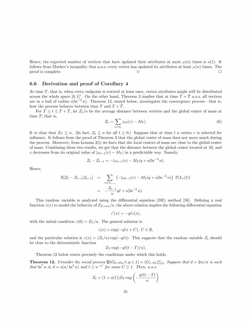
Hence, the expected number of vertices that have updated their attributes at most ω(n) times is o(1). Itfollows from Markov’s inequality that a.a.s. every vertex has updated its attributes at least ω(n) times. Theproof is complete. 3

6.6 Derivation and proof of Corollary 4

At time T , that is, when every endpoint is rewired at least once, vertex attributes might still be distributedacross the whole space [0, 1]r. On the other hand, Theorem 3 implies that at time T + T a.a.s. all verticesare in a ball of radius o(ln−2 n). Theorem 12, stated below, investigates the convergence process—that is,how the process behaves between time T and T + T .

For T ≤ t ≤ T + T , let Zt/n be the average distance between vertices and the global center of mass attime T ; that is,

Zt =∑v∈Vt

|ωt(v)−MT |. (6)

It is clear that ZT ≤ n. (In fact, Zt ≤ n for all t ≥ 0.) Suppose that at time t a vertex v is selected forinfluence. It follows from the proof of Theorem 3 that the global center of mass does not move much duringthe process. Moreover, from Lemma 2(i) we have that the local centers of mass are close to the global centerof mass. Combining these two results, we get that the distance between the global center located at Mt andv decreases from its original value of |ωt−1(v)−MT | in a predictable way. Namely,

Zt − Zt−1 = −|ωt−1(v)−MT |q + o(ln−2 n).

Hence,

E[Zt − Zt−1|Zt−1] =∑

v∈Vt−1

(−|ωt−1(v)−MT |q + o(ln−2 n)

)P(Lv(t))

= −Zt−1

nq`+ o(ln−2 n).

This random variable is analyzed using the differential equation (DE) method [58]. Defining a realfunction z(x) to model the behavior of ZT+xn/n, the above relation implies the following differential equation

z′(x) = −q`z(x),

with the initial condition z(0) = ZT /n. The general solution is

z(x) = exp(−q`x+ C), C ∈ R,

and the particular solution is z(x) = (Zt/n) exp(−q`x). This suggests that the random variable Zt shouldbe close to the deterministic function

ZT exp(−q`(t− T )/n).

Theorem 12 below states precisely the conditions under which this holds.

Theorem 12. Consider the social process P(G0, ω0, `, q, r, 1) = (Gt, ωt)∞t=0. Suppose that d = 2m/n is such

that ln7 n d = o(n/ ln3 n) and ` ≥ n−C for some C ≥ 1. Then, a.a.s.

Zt = (1 + o(1))ZT exp

(−q`(t− T )

n

)

31

for every t such that T ≤ t ≤ T + tf , where T is defined in (1) and

tf =n

q`

(ln lnn− ln

(n

ZT

)).

Since ZT+tf = n/ lnn, this theorem tells us that, a.a.s., the random variable Zt is well concentrated

around the solution of the differential equation until it reaches the value of n/ lnn. Note that tf ≤ T . Itshould be noted that Corollary 4, stated in the main paper, holds under this Theorem with Zt replaced byWt.

Before moving to a proof of Theorem 12, one more useful tool is needed: the “stopping time.”A stopping time with respect to a random process is a random variable S with values in 0, 1, . . . ∪∞

for which it can be determined whether S = t, for any time t, from knowledge of the process up to andincluding time t. The name can be misleading, since a process does not necessarily stop when it reachesa stopping time. The key result says that if a supermartingale (Xi) is stopped at a stopping time (thatis, (Xi) becomes static for all time after the stopping time), then the result is a supermartingale; see, forexample, [58] for more details.

Theorem 13. If, with respect to some process, (Xi) is a supermartingale and S is a stopping time, then(Xmini,S) is also a supermartingale with respect to the same process.

Now, we are ready to prove Theorem 12:

Proof. Since the random variable Zt does not change during rewiring steps, we focus on influence steps only.Suppose that the influence process occurs at times T ≤ s1 ≤ s2 ≤ . . . ≤ st ≤ . . .. Put X0 = ZT and fort > 0, let Xt = Zst . We need to transform Xt into something close to a martingale. Consider the followingrandom variable

Ht = lnXt +qt

n

and the stopping time

S = mint ≥ 0 : Xt <

n

2 lnn∨ t = tf `

.

(Note that Ht is chosen so that it is close to a constant along every trajectory of the differential equationz′(x) = −qz(x).)

Consider the sequence of random variables (Ht : 0 ≤ t ≤ tf `). In order to use the generalized Hoeffding-Azuma inequality (see Lemma 10), we need to estimate the expected change:

E[Ht −Ht−1 | Xt−1, t− 1]

=∑

v∈Vst−1

(ln(Zst−1 − |ωst−1(v)−MT |q + o(ln−2 n)

)− lnZst−1 +

q

n

)

· P

Lv(st)∣∣∣ ⋃

v∈Vst−1

Lv(st)

=q

n+

1

n

∑v∈Vst−1

ln

(1−|ωst−1

(v)−MT |q + o(ln−2 n)

Zst−1

).

32

By Taylor expansion,

E[Ht −Ht−1 | Xt−1, t− 1]

=q

n+

1

n

∑v∈Vst−1

(−|ωst−1

(v)−MT |q + o(ln−2 n)

Zst−1

+O

(1

Z2st−1

))

=q

n+

1

n

(−

∑v∈Vst−1

|ωst−1(v)−MT |q

Zst−1

)+ o

(1

Zst−1ln2 n

)

= o

(1

Xt−1 ln2 n

)= o

(1

n lnn

),

provided S > t, since then Xt−1 ≥ n2 lnn . Similarly, we get that

|Ht −Ht−1| ≤ | ln(Xt−1 − 1)− lnXt−1|+q

n

= O

(1

Xt−1

)+q

n= O

(lnn

n

),

provided S > t again.Therefore, with i ∧ S denoting mini, S, we have

E[Ht∧S −H(t−1)∧S | Xt−1, t− 1] = o

(1

n lnn

)and

|Ht∧S −H(t−1)∧S | = O

(lnn

n

).

Now we may apply Lemma 10 to the sequence (Ht∧S : 0 ≤ t ≤ tf `), and symmetrically to (−Ht∧S : 0 ≤ t ≤tf `), with ε = 1/ lnn, β = o(1/(n lnn)), and γ = O(lnn/n) to show that a.a.s. for all t with 0 ≤ t ≤ tf ` wehave

|Ht∧S −H0| = o(1).

(Note that there are L ≤ tf ` ≤ T ` = O(n lnn) steps and so Lβ = o(1).) As H0 = lnX0, it follows from thedefinition of Ht, that a.a.s. ln(Xt/X0) = −qt/n+ o(1) for 0 ≤ t ≤ S, and thus

Xt = (1 + o(1))X0 exp

(−qtn

). (7)

Now, we will show that a.a.s. S = tf `. The events asserted by the equation hold a.a.s. up until time S,as shown above. Thus, in particular, a.a.s.

XS = (1 + o(1))X0 exp

(−qSn

)≥ (1 + o(1))ZT exp

(−qtf `

n

)= (1 + o(1))

n

lnn

33

which implies that S = tf a.a.s., and so a.a.s. (7) holds for 0 ≤ t ≤ tf `.To complete the proof, it is enough to show that the concentration for the random variable Xt implies

the concentration for the original random variable Zt. Fix t such that T ≤ t ≤ T + tf . It follows easily fromthe Chernoff bound (3) that w.e.p. from time T until time t there are (t−T )`+O(n2/3) time steps at whichinfluence processes are performed. As a result w.e.p.

Zt = X(t−T )`+O(n2/3)

= (1 + o(1))X0 exp

(−q(t− T )`

n+ o(1)

)= (1 + o(1))ZT exp

(−q(t− T )`

n

),

and the proof is finished. 3

6.7 Proof of Theorem 5

Theorem. Consider the evolutionary process P(G0, ω0, `, q, r,K) = (Gt, ωt)∞t=0. Suppose that d = 2m/n is

such that ln7 n d = o(n/ ln3 n) and ` ≥ n−C for some C ≥ 1. Then, a.a.s. for every pair u, v ∈ Vt wehave

|ωt(u)− ωt(v)| ≤√r(

1− q

13K12n lnn

)b`(t−T )/(3n lnn)c

≤√r exp

(−qb`(t− T )/(3n lnn)c

13K12n lnn

)for every t such that T ≤ t = O(`−1n2 ln2 n) (the random variable T is defined in (1)). In particular, ift = cq−1`−1n2 ln2 n for some constant c > 0, then a.a.s. for every pair u, v ∈ Vt we have

|ωt(u)− ωt(v)| ≤ (1 + o(1))√r exp

(− c

39K12

).

Proof. As always, we assume that r = 1 and that at some time t0 ≥ T all vertices lie in the interval [0, 1].(Note that if the maximum distance in each dimension is at most x, then the maximum distance is atmost

√rx.) Let ε = (12K12n lnn)−1. The proof strategy is to show that during at most 3`−1n lnn steps

the interval shrinks by a factor of at least (1 + o(1))qε (that is, the length of the interval will be at most1− (1 + o(1))qε). Since the time intervals can be treated independently, the result follows.

Let us consider the following two cases.Case 1: for every t0 ≤ t ≤ t2 := t0 + 1.5`−1n lnn, we have Mt ≥ K6ε. It follows from Lemma 2(ii) that

w.e.p. for every t in the range under consideration and v ∈ Vt,

Mt(v) ≥ (1 + o(1))K−6Mt ≥ (1 + o(1))ε.

Hence, all vertices selected (during the influence process) between time t0 and t2 are moved away from 0; infact, the distance from 0 is at least (1 + o(1))qε. Since during this time interval there are (1.5 + o(1))n lnninfluence steps w.e.p., all vertices are selected at least once w.e.p. After that, all vertices are in the interval[(1 + o(1))qε, 1] and the result holds.

34

Case 2: for some t1 such that t0 ≤ t1 ≤ t2 := t0 + 1.5`−1n lnn, we have Mt1 < K6ε. Our goal is toshow that the global center of mass cannot drift too fast to the other end of the interval during another1.5`−1n lnn steps. Since Mt1 < K6ε, at time t1 there are at most 2K6εn vertices at distance at most 1/2from 1, the other end of the interval. We will call these vertices red ; the remaining ones are blue. We willcouple the original process with the one in which all red vertices are moved (at time t1) to 1/2. This is theonly difference between the two processes; everything else remains the same, including the rewiring processon the (random) graph Gt. Let ω′t(v) denote the position of vertex v at time t in the coupled process;similarly, M ′t(v) is the corresponding local center of mass of v at time t. We have ωt1(v) = ω′t1(v) for all bluevertices; and ω′t1(v) = 1/2 ≤ ωt1(v) for all red ones.

We consider both processes starting from time t1. First, we will show (by induction on i) that afteri < 1.6n log n influence steps we have the following two properties w.e.p.:

i) for every blue vertex we have |ωt(v)− ω′t(v)| ≤ 2K12εi,

ii) for every red vertex we have |ωt(v)− ω′t(v)| ≤ 1/2.

The property trivially holds for i = 0. Suppose that the property holds for some i and vertex v is selectedfor the influence process at time t. All remaining vertices do not move (in both processes) and so one needsto show the desired property for v only. It follows that w.e.p.∣∣Mt−1(v)−M ′t−1(v)

∣∣ ≤ 1

|Nt−1(v)|∑

u∈Nt−1(v)

∣∣ωt−1(u)− ω′t−1(u)∣∣

≤ 1

|Nt−1(v)|

((2K12εi)(# of blue neighbors)

+(1/2)(# of red neighbors))

≤ 1

|Nt−1(v)|((2K12εi|Nt−1(v)|) + (1/2)(2K12ε|Nt−1(v)|)

)≤ 2K12ε(i+ 1),

since w.e.p. there are at most 2K12ε|Nt−1(v)| red neighbors of v. Indeed, by the upper and lower boundsfor the probability of an edge, there are at most 4K8mε/n red neighbors, and the size of the neighborhoodin total is at least d/K4 = (2m)/(nK4). Hence the fraction of red neighbors is at most 2K12ε. It followsthat w.e.p. for each blue vertex we have

|ωt(v)− ω′t(v)| ≤ q|Mt−1(v)−M ′t−1(v)|+ (1− q)|ωt−1(v)− ω′t−1(v)|≤ q2K12ε(i+ 1) + (1− q)2K12εi ≤ 2K12ε(i+ 1).

Similarly, w.e.p. for each red vertex we have

|ωt(v)− ω′t(v)| ≤ q|Mt−1(v)−M ′t−1(v)|+ (1− q)|ωt−1(v)− ω′t−1(v)|≤ q2K12ε(i+ 1) + (1− q)(1/2) ≤ 1/2,

where the last inequality follows by our assumption on i. The claim holds by induction.We consider 1.5`−1n lnn steps of the process which selects all vertices w.e.p. Clearly, in the coupled pro-

cess the global center of mass is always in the interval [0, 1/2] (deterministically). Since (2K12ε)(1.5n lnn) <

35

1/3, w.e.p. blue vertices in the original process are close to their counterparts in the coupled one: Indeed, sincethe difference of the global center of mass coming from the contribution of red vertices is at most 2K6ε, andthe contribution coming from blue vertices at most 1/3, the global center of mass in the original process mustbe smaller than 5/6+2K6ε w.e.p. But this implies that once all vertices are selected for the influence process,all of them must be far away from 1: By Lemma 2(ii) we then have that Mt(v) ≤ 1− (1 + o(1)) 1

6K−6 + o(1).

Hence, the distance of Mt(v) from the right border of the interval is at least 16K−6 + o(1), and once the

vertex undergoes the influence process, its distance from the right border is thus at least q 16K−6 + o(1). The

proof is finished. 3

36