HONG KONG INSTITUTE FOR MONETARY … Hong Kong Institute for Monetary Research, its Council of Advisers, or the Board of Directors. Acknowledgments: We thank Jean-Louis Arcand, Marius

HONG KONG INSTITUTE FOR MONETARY RESEARCH

THE CONSUMPTION RESPONSE TO MINIMUM WAGES: EVIDENCE FROM CHINESE HOUSEHOLDS

Ernest Dautovic, Harald Hau and Yi Huang

HKIMR Working Paper No.24/2017 November 2017

Hong Kong Institute for Monetary Research 香港金融研究中心 (a company incorporated with limited liability)

All rights reserved.

Reproduction for educational and non-commercial purposes is permitted provided that the source is acknowledged.

The Consumption Response to Minimum Wages:

Evidence from Chinese Households

Ernest Dautovic*

University of Lausanne

Harald Hau

University of Geneva and Swiss Finance Institute

Yi Huang Graduate Institute Geneva

November 2017

Abstract

This paper evaluates the Chinese minimum wage policy for the period 2002-2009 in terms of its impact

on low income household consumption. Using a representative household panel, we find support for

the permanent income hypothesis, whereby unanticipated and persistent income increases due to

minimum wage policy change are fully spent. The impact is driven by households with at least one

child. We infer significant positive welfare effe cts for low income households based on expenditure

increases concentrated in health care and education, whereas a negative employment effe ct of higher

minimum wage cannot be confirmed.

Keywords: Minimum wages; Labor income; Household consumption; Permanent income hypothesis

JEL classification: E24, J38, C26

*Email addresses: Ernest: [email protected], Harald: [email protected] and Huang: [email protected]

The views expressed in this paper are those of the authors, and do not necessarily reflect those of the Hong Kong MonetaryAuthority, Hong Kong Institute for Monetary Research, its Council of Advisers, or the Board of Directors.

Acknowledgments: We thank Jean-Louis Arcand, Marius Brulhart, David Card, Eric French, Wei Huang, Gian-Paolo Klinke,Olivier Cadot, Rafael Lalive, Albert Park, Dominic Rohner, Li Shi, Stephanos Vlachos, Gewei Wang, Shangjin Wei for valuablecomments on earlier drafts of the paper. We also thanks seminar participants at the research days of the Faculty of Businessand Economics at the University of Lausanne. This research project benefited from a Sinergia Research Grant from the SwissNational Science Foundation (SNSF).

1 In the development economics literature consumption is the standard measures to assess the relative poverty of households. The World Bank relies on consumption measures to construct the international extreme poverty line, recent update brings it to $1.25 per day at purchasing power parity (PPP) rates, Ravallion et al. (2009).

2 For the effects of minimum wages on employment in the U.S. see for example the contributions of Krueger and Card (1995) and Card and Krueger (2000) juxtaposed to Neumark and Wascher (1992) and the recent evidence of Dube et al.(2010), Allegretto et al. (2011), Neumark et al. (2014a), Neumark et al. (2014b), Allegretto et al. (2016). The literature on the employment effect of minimum wages in developing countries is briefly surveyed in Section 6.

1

Hong Kong Institute for Monetary Research Working Paper No.24/2017

1. Introduction

Minimum wage policies are among the most controversial public policies not only in developed coun-

tries, but also in emerging economies. In China, the minimum wage policy has been reformed after 2003

and enforced throughout a labor market with more than 800 million workers. But how effec-tive were

these minimum wage policies in improving income, consumption and welfare of low income households?

This paper analyzes the effect of the minimum wage level on consumption spending in a repre-sentative

panel of Chinese households for the period 2002-2009. Household consumption provides a particularly

relevant metric of welfare because it is often better measured and less volatile than income, Deaton

(1997), Deaton and Grosh (2000).1 The effectiveness of minimum wage policies in developing countries

has been questions for fears about unemployment risk, threats to an already precarious industrial

competitiveness, and employment substitution into the informal labour market, Rama (2001), Fang and

Lin (2015). And there are additional concerns why higher minimum wages may fail to translate into higher

levels of consumption: first, higher minimum wages may simply sub-stitute for other social transfers so

that the effective income increase is considerably attenuated. Many social transfer programs are

conditioned by income thresholds and cumulative effect of ineligibility is hard to evaluate in practice.

Second, the disposable income effect of higher minimum wages may be perceived as transitory -

particularly in emerging countries with higher price inflation. Consumption smoothing may then result only

in modest consumption and welfare increase. Third, higher minimum wages may increase unemployment

risk, raise precautionary saving and again attenuate the consump-tion effect. Fourth, the higher

frequency of unemployment can make some households much worse off than in the previous policy

regime.2

Against the background of these concerns, our study is the first to estimate the consumption and income

response of Chinese households to the large cross-sectional and intertemporal variation of China’s

minimum wages. For the period 2000-2009, we identify more than 13,874 changes in the local minimum

wage across China’s 2,183 counties and 285 cities and match them to the urban household survey

(UHS) which covers 73,164 urban household-year observations. The study finds that minimum wage

increases in China functioned as a very effective tool for increasing the consumption level of low income

households. Similarly to the evidence from the U.S., Neumark and Wascher (2011), local minimum wage

hikes complement (rather than substitute) other social transfers so that labor income and transfer income

often tend to increase simultaneously in minimum wage recipient households. The

measured total income effect is thereby magnified: RMB 1,000 labor income increase due to a minimum

wage hike implies RMB 1,500 labor income increase in poorest households due to multiple minimum

wage earners within a family and comes with an additional average RMB 1,000 in transfer income. This

suggests that local minimum wage increases in China are part of a more comprehensive social policy

change toward low income households. It is consistent with local political leaders’ promotions which

hinge primarily on economic performance of their county. At the same time, high income households do

not experience commensurate increases in their transfer income whenever minimum wages raise.

Second, we show that low income households spend the entire additional income coming from a higher

minimum wage. As the minimum wage shock itself is difficult to predict and the associated income effect

highly persistent, we can interpret this evidence as confirmation of the permanent income hypothesis.

We perform both reduced form estimations, which relate consumption changes directly to the increase in

the annual minimum wage, as well as two-stage least square estimations (2SLS), which use the

minimum wage increase as an instrument for household income in the consumption function. Both

methods provide consistent results and do not reject the permanent income hypothesis. The

consumption elasticity to (permanent) income does not differ significantly when we consider liquidity

constrained households. Only households without a child feature significantly lower consumption

elasticity, which points to higher old-age savings.

The literature on the effects of minimum wages on consumption is scant, particularly for developing

countries. A few studies have investigated the impact of minimum wages on durable and non-durable

consumption for U.S. states. Aaronson et al. (2012) estimate a positive expenditure effect for mini-mum

wage dependent U.S. households, and conclude that most of the consumption is due to vehicle

purchases. Similarly, Alonso (2016) employs sales data to find that a 10% increase in minimum wages

increases non-durable consumption by 1% at an aggregate county level, and shows that the increase is

greater in poorer counties. The effect of minimum wage changes on other wages and labor income in

developing countries is better documented. Using labor survey data from Indonesia, Rama (2001)

estimates the impact of doubling the minimum wage on the entire wage distribution, and finds that

wages above the minimum wage also increased between 5-15%. Bosch and Manacorda (2010) find that

all growth inequality in income earnings in Mexico is due to the decline in the real value of the minimum

wage. Engbom and Moser (2016) study the impact of the minimum wage change in Brazil on the

reduction of earnings inequality and conclude that minimum wages help reduce earnings inequality in

formal sectors of the economy and that the decline is more pronounced at the bottom of the wage

distribution.

Research on developing countries has generally considered alternative income shocks to estimate

consumption elasticities. Wolpin uses weather induced income shocks in India to estimate a con-

sumption elasticity to income in the range 0.91-1.02 depending on the definition of consumption.

2


Related work by Paxson studies weather shocks in Thailand to estimate the saving propensity to income

shocks related to weather conditions; the estimated saving propensity to positive and persis-tent weather

shocks is found to be greater than zero, but small. Nevertheless, while weather shocks or other disasters

can have relatively persistent income effects, they may not always amount to permanent income

changes.

Negative employment effects of minimum wage increases have always been a key policy concern. In the

Chinese context, we do not find that higher minimum wages increase unemployment in urban low

income households. While various point estimates for the employment elasticity of high mini-mum wages

are negative, their economic and statistical significance remain low across various model specifications.

This absence of negative employment effects could be explained by the extremely low minimum wage

level in China, which is generally below 20% of the median wage compared to around 30% in the U.S. or

up to 60% in France and Sweden, Dickens (2015). At such a low minimum wage level, even low

productivity workers can typically find a new job after being fired. Evidence of a higher turnover rates in

counties with an increase in minimum wages supports this interpretation. 3

The effect of minimum wages on employment in China is disputed. Using firm-level data from border

regions subject to different minimum wage changes, Huang et al. (2014) find a small and negative

relation between Chinese minimum wages and firm employment. However, employment flows out a firm

sample may not be synonymous with more unemployment. Unlike household survey data, firm-level data

cannot not track the employment history of a worker. Fang and Lin (2015) find small negative

employment effects of minimum wages using the Chinese urban household panel. Their estimated

employment elasticity to minimum wage hikes is -0.05 in the full sample and -0.09 among young adults.

However, these results appear fragile to the inclusion of county-level trends, which the authors do not

account for.

Our paper is organized as follows. Section 2 explains China’s minimum wage regulation, the persistence

in the behavior of real minimum wages and the urban household survey. Section 3 discusses the

research design. Section 4 presents the main results on the impact of minimum wage level on total

household consumption. Here we also highlight the important role of minimum wages in determining a

household’s health and education expenditure. The role of household heterogeneity for consumption

behavior is discussed in Section 5 with a focus on financial constraints and family structure. Section 6

explores the effect of minimum wages in explaining (un-)employment and job turnover for low wage

workers. In Section 7, we run a placebo test and Section 8 concludes.

3 Moreover, developing countries feature much larger informal labor markets, which can absorb workers who have lost their job in the formal sector, Comola and De Mello (2011). Meghir et al. (2012) elaborate on this mechanism in a labor market model with search frictions.

3


2. Data2.1 Minimum Wage Regulation and Behavior

Chinese minimum wage legislation was first enacted in 1994 following a wave of economic liberalization

policies and the transition from predominantly state-owned production to a mixed economy with a

growing private sector. Its implementation was poor and it lacked provisions and rules for the adjustment

to price inflation and local economic conditions. It also suffered from lax enforcement and non-

compliance. Rawski (2003), Du and Wang (2008), Zhongwei and Binbin (2011), Ye et al. (2015).

In December 2003, the central government opted for a reform of minimum wage regulation. Fol-lowing

China’s access to the World Trade Organization in 2002, the ensuing increase in foreign direct investment

and the related boom of the manufacturing sector added pressure for stricter minimum wage regulation.

In March 2004, the Ministry of Labor and Social Security introduced the new Min-imum Wage Regulations

(MWR) into Chinese Labor Law. The most significant provisions required indexation of the minimum

wage to the cost of living and a minimum wage level sufficient to support basic daily needs of employees.

Local authorities were required to review the minimum wage at least every two year in light of local

economic conditions and propose a revised minimum wage to the provincial authorities.4 Moreover,

implementation of the new MWR was strengthened by increased control at the local administrative level

and firm level in pursuit of better compliance. Penalties for non-compliance increased from 20-100% of

the statutory minimum wage to 100-500%.

The data used in this study were collected by Chinese Ministry of Human Resources and report the local

minimum wage in 2,183 counties and 285 cities for the period 1994-2012. The main variable of interest is

the hourly minimum wage imposed in a county or city. The hourly rate can be extrapolated to an effective

monthly minimum wage adopting a standard 40 hours working week as stipulated in Article 33 of the

Chinese Labor Law.5 To match the minimum wage data to the annual frequency of the household survey,

we construct an annual real minimum wage by averaging effective monthly real minimum wages.

In line with the new MWR, large productivity growth and a booming manufacturing sector, real

minimum wage growth in China was 8.7% in the period 1996-2003 and accelerated to 12.8% in

the period 2004-2012. The average annual real minimum wage was only RMB 1,259 ($441 under

PPP) in 1996, but had increased to RMB 4,610 ($1,309 under PPP) in 2012.6 In the same

period, the annual real growth rate of Chinese labor productivity was 8.9%, while real GDP oscillated

around 9.7%.7

4 The province is the highest administrative division in China, followed by cities and counties. There are 34 provinces in the Chinese administrative subdivision as of April 2015, 333 prefecture-level cities and a total of 2,862 county-level divisions in China.

5 Details on Chinese Labor Law can be consulted at: http://www.china.org.cn/living_in_china/abc/2009-07/15/content_18140508.htm

6 Effective annual nominal minimum wage increased from RMB 2,628 ($921 under PPP) in 1996 to RMB 13,224 ($3,756 under PPP) in 2012.

7 Purchasing power parity conversion factors are from the World Bank’s International Comparison Program Database,4


http://www.china.org.cn/living_in_china/abc/2009-07/15/content_18140508.htm

http://www.china.org.cn/living_in_china/abc/2009-07/15/content_18140508.htm

In other terms, China’s average real minimum wage started slightly above the international poverty

line set at $1 per day in 1996, and increased to a remarkable $3.55 per day in two decades.

Table 1 illustrates that Chinese minimum wages are generally set at very low levels relative to the median

wage. The average ratio of the minimum wage relative to the median wage (also referred to as the

minimum wage “bite”) fluctuates around 20% in the period 2002-2006 and then declines to 17.6% in

2009. Minimum wages never approached the much higher levels observed in some developed countries,

where the minimum wage bite ranges from around 30% in the U.S. to 60% in France and Sweden,

Dickens (2015). Therefore, the labor income and living conditions of minimum wage workers in China are

much worse in relative terms compared to minimum wage workers in high income economies. In absolute

terms, the Chinese minimum wage income of a single worker is close to the international poverty line: it

follows that any policy measure that increases the consumption level of these extremely poor households

represents a reduction in severe poverty.

Importantly, for the evaluation performed in this study minimum wages in China were subject to large and

heterogeneous local variation. Our empirical analysis focuses on the years 2002-2009 for which the urban

household data is available as a stratified panel and can be matched with county-level minimum wage

data. During this period, 79.5% of all county-year events increased their minimum wage in a given year,

this translates in 13,874 episodes of minimum wage increases in Chinese counties over the period and is

the main source of variation the study exploits. Figure 1 presents a diagram with the annual share of

counties and cities that change the nominal minimum wage in the range of 0-20% or more than 20%.

During the period almost one quarter of China’s 2,183 counties and 285 cities in the sample raised the

nominal minimum wage by more than 20%. At the same time none of the counties featured a decrease in

the nominal wage, local inflation combined with a constant minimum wage can however decrease the real

wage, and from 2002 to 2009 an average of 20.5% (3590) county-year events had nominal minimum

wage constant implying a worsening of purchasing power of minimum wage workers. Yet, most local

authorities appear attentive to the erosion of the minimum wage by inflation and tend to adjust the

minimum wage by more than the rise in consumer prices: of the 13,874 county-year events with a

minimum wage increase, only 1,235 had minimum wage increases below the inflation rate in the county.8

A final issue concerns the persistence of real minimum wage changes. Even if nominal minimum wage

change are unlike to be reversed, inflation can induce the mean reversion of the real minimum wage. If,

on the other hand, real minimum wages feature a high degree of persistence, then an increase in the

minimum wage is closer to a permanent income increase. To explore the intertemporal data on growth

are from the World Bank World Development Indicators, productivity data are from the OECD.stat

Productivity Archives.

8 In real terms, approximately half of county-year increases implied a real minimum wage change in the range 0-10%, one-third of minimum wage increases was in the range 10-20%, and only a tenth above 20%.

5


persistence of real minimum wage increases, we run the regression

∆MWc,t = α0 + ρMWc,t−1 + a1t+ δp,t + γc + εc,t, (1)

where a coefficient ρ < 0 captures mean reversion to a time trend t of the real minimum wage MW; δpt

denotes a province-year fixed effect and γc a county fixed effect.

Table 2 reports the regression results for the period 1992-2012 and the shorter sample period 2002-2009

corresponding to time frame of our analysis. We progressively augment the specification with county fixed

effects and county trends to mitigate the impact of cross-sectional dependence. The coefficient of interest

ρ is in general negative and statistically significant. Yet, the magnitude of the mean reversion is

economically weak. For example, the coefficient in Column (4) implies a half-life of 5.47 years for the real

minimum wage.9

Unit root test adapted to panel data can also be used to test for real minimum wage persistence in a

narrow statistical sense, Harris and Tzavalis (1999) . Under the null hypothesis of a unit roots (i.e. the

real minimum wage increase is permanent) such tests provide a critical value for ρ below which the unit

root cannot be discarded. The H-T test fails to reject the null hypothesis when we don’t demean the real

minimum wage to take into account cross-county dependence. However, when we compute in each time

period the mean of the minimum wage across counties and subtract this mean from the series the test

rejects the null.10 Economically, real minimum wage changes exhibit a large degree of persistence even if

the unit root hypothesis can be rejected in some specifications.

Another important issue is the extent to which a change in the minimum wage can be predicted by

Chinese households. Generally, county-level changes in the real minimum wage are very difficult to

predict so that minimum wage change can be interpreted as an unanticipated income effect. Appendix A

shows with a wide range of tests that the decision to change the minimum wage is not predicted by

standard socio-economic and political determinants. In conclusion, the high persistence and low

predictability of the minimum wage change imply that minimum wage changes in Chinese cities and

counties are akin to unanticipated permanent income shocks to low income households. This allows us to

interpret the resulting consumption response of households as a test of the permanent income

hypothesis.11

9 Half-life is computed adjusting the standard formula to take into account that we are using the first difference of the minimum wage as dependent variable: ln(0.5)/ln(−0.119 + 1) = 5.471. Using the coefficient in Column (8) implies a half-life of 2.31 years.

10 To corroborate these findings, we also undertake the Im et al. (2003) test, which relaxes the assumption about the common autoregressive coefficient and runs the test for each cross-section under the null that all panels have unit roots, against the alternative that some panels are stationary. This test fails to reject the null hypothesis except when we include a time trend and demean the series to reduce the influence of cross-section dependence.

11 There is a vast literature testing the validity rather than the failure of the permanent income hypothesis in different setting and countries, exploring the reasons for this failure like for example liquidity constraints. The review of this literature is beyond the scope of this paper, however the interested reader can refer to the excellent review by Jappelli and Pistaferri (2010).

6


2.2 China’s Urban Household Survey

China’s Urban Households Survey (UHS) represents a comprehensive and representative survey of urban

workers and households managed by the Chinese National Bureau of Statistics (NBS). The UHS is

conducted via stratified randomization sampling, records a wide range of demographic and socioeconomic

conditions of Chinese urban households, including detailed information on different income sources,

wages and granular consumption items for households. In this paper, we restrict our analysis to eight

consecutive years of the UHS from 2002 to 2009. Prior to 2002, the survey does not provide a panel

structure and we exclude the earlier years from the econometric analysis. We then merge the urban

household survey with the minimum wage data. Appendix B provides a detailed description of the merged

sample and the data filters applied.

To analyze the impact of minimum wages on household consumption, we divide households in terms of

their reliance on wage income near the local minimum wage. Let the variable S denote the share of total

non-property income earned by the two best-paid household members due to a wage near the minimum

wage.12 Labor income of any household member is considered to be near the local minimum wage and

counted towards the nominator of S if it falls within the range 50%-150% of the county minimum wage. We

calculate the share S for the first year a household enters the survey to limit any endogeneity due to self-

selection or composition effects.13 We include in the sample households that have been surveyed for at

least two years and that have at least two household members observed in each survey. Formally, let

Em,h,c denote the annual labor income and wm,h,c the wage of the two best paid household members m

= 1, 2 in household h in county c. For a dummy variable D[.] = 1 indicating a wage in the range 50%-150%

of county minimum wage MWc, we define minimum wage income share as

where Total Incomeh,c in the denominator represents the sum of the total disposable income of the

two top earners in the household.14 By definition, the minimum wage income share Shc is between 0 and

1; a higher share implies that the household tends to be poorer and more subject to any variation in the

minimum wage. In the case where both the household head and spouse work at the minimum wage,

the share S approaches one.15 Throughout our analysis, we consider households without any

12 See Aaronson et al. (2012) for a similar definition.

13 The upper bound of 150% is consistent with the findings of spillover/ripple effects of minimum wages on the wage distribution

14

7

15

Sh,c =1

Total Incomeh,c

∑m=1,2

Em,h,c ×D [0.5MWc ≤ wm,h,c ≤ 1.5MWc] (2)

whereby workers earning just above the minimum wage tend to have an upgrade when the minimum wage is increased, Krueger and Card (1995). The results are robust to other thresholds for minimum wage ripple effect (0.5-1.2 and 0.5-1.3) and to other definitions of the treatment, that is whether or not we assign the treatment in the first year a person is sampled or, alternatively, we allow for assignment to treatment only if the worker earns a minimum wage in every year is observed.

This is composed by the sum of labor income, property income, operating income and transfer income.

If all members of the household are unemployed in the first year the household enters the panel, the sum of the ”best” two earners results in a zero labor income and consequently S = 0. We eliminate these households from the data set (166 observations or 0.2% of the overall sample) to avoid any confounding effe cts with households earning labor income above the minimum wage.


minimum wage income (S = 0), the complementary set of households with at least some income

related to the minimum wage (S > 0), households with at least half of their income from wages

near the minimum wage (S > 0.5), and households very dependent on the minimum wage for their

subsistence (S > 0.75). The last two groups are the focus of our interest and we can expect the

consumption response to minimum wage changes to be most pronounced here.

It is instructive to compare household characteristics across the four different household groups (S = 0, S

> 0, S > 0.5 and S > 0.75) that vary their dependence on minimum wage income. Table A4 in Appendix B

reports the differences in the structure of household income and spending and Table A5 the differences in

demographic structure.

Households with S > 0.5 (S > 0.75) account for 6% (5%) of all observations, but earn only

2.6% (2.4%) of all labor income, whereas households without minimum wage income represent 72%

of the sample and earn 81.9% of all labor income. Generally, poorer households (with S > 0.5 or

S > 0.75) feature a lower share of disposable income earned from labor income and rely more on

social transfer income from the authorities; almost 20% of their disposable income comes from

social transfers. Moreover, minimum wage dependent households tend to consume a

higher proportion of their disposable income (82%) compared to other households with S = 0 (70%).16

In terms of demographic characteristics, minimum wage households tend to be only slightly larger

with 3.3 members compared to 3.1 for the household S = 0, this fact suggests that the one child

policy was implemented consistently across income groups. Unsurprisingly, minimum wage household

show lower house ownership rates and their migration to the urban area is typically more recent. We

also highlight that minimum wage dependent households are much less likely to work for state-owned

enterprise (SOE), these tend to pay higher wages than the private sector. Finally, the

educational level and work experience of the head of household tends to be lower for

minimum wage dependent families.

3. Research Design

3.1 Is There a Correlation Between Consumption and Minimum Wage Changes?

Before we explore the causal link from minimum wages to household consumption, it is useful to

estab-lish that minimum wages and consumption correlate only for minimum wage dependent

households. Many economic channels could potentially generate spurious correlations between both

variables and 16 In Table A4 and throughout the analysis, consumption is defined as expenditure on: food, clothes, household services, medical

care, education, transportation and living. This is consumption net of purchasing property, transfer expenditures, social contributions and personal social expenditure. It is also net of investments, these can be confounded as savings.

8


make it harder to disentangle the causal effects of minimum wages on consumption. To convince the

reader that such spurious correlations do not obstruct our analysis, we apply a simple two-step procedure.

First, we generate residuals which identify if the minimum wage level is high relative to the province average, in a first-stage regression of the county-level real minimum wage MWct in year t on a set of interacted province fixed effects DProvince and year fixed effects DY ear. Formally,

MWc,t = α0 + α1 [DProvince ×DY ear] + uc,t, (3)

where the residuals uc,t identify the real minimum wage level in a county relative to the province average.

The residual value is positive (negative) if a county has a minimum wage level higher (lower) than the

average minimum wage level in its province for a given year. In a second step, we fit household

consumption change with the residual county changes ∆uc,t, if there is a poitive correlation between the

minimum wage change and consumption this should appear only for households depending on minimum

wages. To visually inspect this fit we sort the residual county changes ∆uc,t into bins b of 40 counties and

calculate the bin average ∆ub for each bin b. Accordingly, we calculate for all counties in each bin, the

corresponding average changes of household consumption ∆Cb. In this aggregation, we distinguish

minimum wage dependent households (S > 0.5) from those without minimum wage income (S = 0) and

therefore averaging within the bins yields average consumption changes ∆CS>0.5b and ∆CS=0

b

Note that, within a bin, the two groups of households share the common minimum wage change ∆ub

∆CS>0.5b = β0 + β1∆ub + ε (4)

∆CS=0b = γ0 + γ1∆ub + ε (5)

where the exogeneity test of the event analysis requires β1 > 0 and γ1 = 0. Consumption changes ∆CS=0b

for non-minimum wage households show a correlation of −0.03 with the relative minimum wage change

∆ub, whereas minimum wage dependent households show a positive correlation of 1.42. A standard t-test

for the statistical difference of the two slopes produces a t-statistic of 1.56. Despite the weak statistical

significance, it can be inferred from the scatter plot that minimum wage increases are indeed associated

with higher household consumption for minimum wage dependent households.

A further refinement of the procedure distinguishes two subsamples: (i) counties in which the nominal

minimum wage was constant from one year to another, (ii) those where local authorities implemented

nominal minimum wage hikes. In the former case, the county minimum wage decreases with respect to

the province-year average, whereas in the latter case the county minimum wages increase relative to the

province average. The implications for household consumption differ in the two subsets: only in counties

9

relative to the province-level average. Figure 2 illustrates the binned scatter plots for the two regressions:


with minimum wage hikes we expect a positive relationship (β1 > 0) between minimum-wage-household

consumption changes and the relative minimum wage change. In Figure 3, we compare the regression

lines for cases (i) and (ii) and confirm the conjectured relationship. Only counties with local minimum wage

increases have a strong correlation between minimum-wage-households consumption change and the

residual change ∆ub. Minimum-wage-households show no consumption changes in counties where the

nominal minimum wage was constant.

Figures 2 and 3 provide descriptive evidence on the relation between minimum wage changes and

consumption changes. Only in counties with local minimum wage hikes do we find a positive correlation

with household consumption changes, and this correlation pertains only to minimum wage dependent

households.

3.2 Panel Data Methods

The large spatial and intertemporal variation of minimum wages across Chinese counties suggest a panel

analysis to identify and estimate consumption elasticity to minimum wage income shocks. The difference in

difference specification compares household consumption across counties with different minimum wage

levels, with households in counties with unchanged minimum wage acting as a control group. In light of the

heterogeneous household exposure to minimum wage income, we segment the household sample into

groups according to their share S of total income received from minimum wage labor. Households without

any minimum wage related income (S = 0) represent an additional control group relative to those

household with S > 0.5 (S > 0.75) which earn more than 50% (75%) of their total income from minimum

wages. The household’s minimum wage dependence thus constitutes the third dimension of differencing.

The household survey data provide a rich set of demographic and socio-economic characteristics

(Xm,h,t) for the two main labor income earners (m = 1, 2) in the households. For the purpose of the

analysis, we use as controls their age and age squared, gender, years of work experience and work

experience squared, years since migration to the city and its squared value. Additional categorical

covariates include marital status, level of education, occupation and industry of occupation. The observed

household characteristics (Xh,t) include family size measured by the number of family mem-bers and a

house ownership dummy. Apart from labor income, we also observe a household’s transfer income, net

operating income from business, lending activity and income from property. At the city level, we dispose of

a variety of macroeconomic variable (Xcity,t): population size, city real GDP, city real average wage and

city unemployment rate. These variables are not available at the more granular county level. But we

generally allow for different growth trends at the county level including the interaction of a county dummy

and a time trend (φc · t) in the regression. The general specification of the household consumption

equation take the reduced form:

10


Ch,c,t = α+ βRFMWc,t + Xm,h,tΛ + Xh,tΘ + Xcity,tΞ + φc · t+ ηh + δp,t + εh,c,t, (6)

where the subscript h characterizes the household, c the county and t the year. The specification also

accounts for household fixed effects ηh and province-year fixed effects δp,t to allow for heterogeneous

economic developments across China’s main geographic regions. All monetary variables, including the

minimum wage, are defined in real terms using the province-level consumer price index. The coefficient of

interest in this reduced form specification is the linear effect βRF of the minimum wage level MWct on

household consumption Ch,c,t.

A more general approach consists relates household consumption to household income by using the

minimum wage change as an instrument to explain variation in household income. This two-stage least

square estimation (2SLS) first explains household labor income using a first-stage regression

Incomeh,c,t = α+ βFS MWc,t + Xm,h,tΛ + Xh,tΘ + Xcity,tΞ + φc · t+ ηh + δp,t + εh,c,t, (7)

and in the second stage relates the predicted income variation Incomeh,c,t induced by minimum wage

variation to account for household consumption, therefore

Ch,c,t = α+ β2SLS Incomeh,c,t + Xm,h,tΛ + Xh,tΘ + Xcity,tΞ + φc · t+ ηh + δp,t + εh,c,t. (8)

The advantage of the 2SLS approach is that it accounts explicitly for the channel through which minimum

wages affect consumption. Intuitively, and conditional on covariates, 2SLS retains only the variation in

household labor income that is generated by the minimum wage instrument, and thus provides a cleaner

estimate of the direct impact induced by the minimum wage change, Angrist and Pischke (2008). The large

and frequent variation of the real minimum wage in China guarantees that the explanatory power of the

first-stage regression is sufficiently large.

The first-stage regression can also provide information which component of household income is affected

by the minimum wage change. For example minimum wage increases can be accompanied with higher

social transfer payment when part of a comprehensive social security benefits policy, so that minimum

wage increases also predict increases in social transfers. Alternatively, minimum wage increases can

crowd-out transfer income if the latter is subject to eligibility requirements that can - inter alia - depend on

the higher labor income. In both cases the impact of the minimum wage on consumption can be biased if

transfers are not included in the specification, empirical evidence shows the importance of social security

benefit programs in helping poorer families smooth their consumption, Romer and Romer (2016). To

control for the complementarity of minimum wage hikes with other social transfer policies a set of

specifications cumulates labor and transfer income in a single dependent variable in the first stage

regression.17

11

17 Transfers are intended net of pension or retirement benefits, our measure of net transfers includes: social assistance income, dismissal compensation, income insurance, income from donations and other transfer income.


The inclusion of county-level time trends φc · t is important for our specification, because we do not dispose

of macroeconomic controls at the county level. If we do not allow for county-specific hetero-geneous trend

growth, the real minimum wage level MWc,t represents the only county level regressor and is likely to

subsume county-level heterogeneity and bias the inference. It is straightforward to illustrate this

specification issue by comparing first-stage income regressions with and without county time trends; the

results are shown in the Appendix Table A6. In the standard two-way specification with only time fixed

effects, but without county time trends and interacted province-year fixed effects, the correlation between

the real minimum wage and household income is highly significant even for the household groups not

earning any minimum wage income (S = 0) as shown in Column (1) of Table A6. By contrast, county time

trends in Columns (5)-(8) in combination with province-year fixed effects capture unobserved

heterogeneity in the economic development across counties and eliminate any con-sumption dependence

of high income households on the level of the minimum wage. As a consequence of this result, we always

present estimates including both linear county trends and province-time fixed effects.

4. Main Results

4.1 First-Stage Income Regressions

Table 3 presents estimates for the first stage regression for different definitions of household income. We

distinguish pure labor income in Columns (1)-(3), transfer income in Columns (4)-(6) and the sum of labor

and transfer income in Columns (7)-(9) as the dependent variables. We consider three household groups:

those that receive at least 25% (S > 0.25), at least 50% (S > 0.5), or at least 75% (S > 0.75) of their total

income from minimum wages, respectively. All specifications include county trends and province-year fixed

effects to account for unobserved heterogeneity. We also report three different types of standard errors:

two-way clustering at county and province-year levels, and two way-clustering at county and city-year

levels. 18

The effect of minimum wages on labor income in Columns (1)-(3) increases in the minimum wage share S

and is significant only for households earning more than half of their disposable income from minimum

wages. The coefficient of 1.56 in Column (3) suggests that income elasticity is larger than one for

households with a strong minimum wage dependence, this can be explained by the presence of multiple

minimum wage earners in the same household. Given the standard error of 0.743, the t-statistic is 2.104

and in principle is a sign of a sufficiently strong instrument.19

18 Two-way clustered standard error allow for arbitrary correlation of residuals due to city/province-wide shocks such as floods, earthquakes or city/province-wide economic policies.

12

19 Note further that a single instrument 2SLS is median-unbiased and hence less prone to weak instrument critique, Angrist and Pischke (2008). A more formal test of the validity and relevance of first stage instruments is from Kleibergen and Paap (2006) and is provided in the 2SLS regressions in Table 5.


More surprising is the large positive predictive effect that minimum wages have for transfer income in the

same household group. A positive coefficient of 1.09 in Column (6) implies that a RMB 1,000 increase in

the annual minimum wage comes with an equally large increase in social transfers. Accordingly, we find

much larger coefficients for the minimum wage effect on the combined labor and transfer income of

households. The total household income effect of minimum wage changes is roughly 2.5 times the

variation in the annual minimum wage at the county level. With a county clustered standard error of 0.729

the t-statistic approaches the value of 3, which with a single endogenous variable and single instrument

translates in an F-statistics close to 10, hence the instrument relevance of the minimum wage is stronger

when used for the sum of labor and transfer incomes as unique endogenous variable. This implies that

using the exogenous shift in minimum wage policy as an instrument for income shock will have a greater

explanatory power when both labor and transfer incomes are instrumented with minimum wage. It follows

that the related 2SLS estimates will be more precisely estimated.

The evidence for transfer income suggests that minimum wage policy in China is one dimension of a more

comprehensive set of policy measures targeting low income families. Thus, the minimum wage hike is an

instrument for additional changes in social transfers that we do not observe directly, can be interpreted as

a social policy measure and proxies for exogenous income effects more generally because it captures

local authorities desire to provide transfer income.

4.2 Reduced Form Regressions

In this section the reduced form estimates for the relationship between the real minimum wage level and

the consumption level in minimum wage dependent households are presented. Table 4 presents two

different specifications. First, Columns (1)-(4) report the standard specification adopted in the minimum

wage literature on the impact of minimum wages on some outcome of interest, Aaronson et al.(2012),

Allegretto et al. (2011) and Neumark et al. (2014a); controls for all non-labor income sources and is

related to the first-stage regression with labor income as the dependent variable. Second, Columns (5)-(8)

exclude transfer income as a covariate and therefore allow the effect of transfer income on consumption

to be captured by the minimum wage change itself. The resulting coefficient is inflated upwards since the

minimum wage estimate captures the residual effect of net transfers. The point estimates have increased

significantly only for households with S > 0.5 suggesting that net transfers have a significant contribution

in terms of consumption exclusively for households with a higher minimum wage dependence. For them,

the relative incidence of net transfers on consumption is substantial given that net transfers constitute less

than 8% of household disposable income, cfr. Table A4 in Appendix B. In both specifications the point

estimate for the annual real minimum wage effect on household consumption increases in the minimum

wage share S of household income. For the households most dependent on minimum wage income (S >

0.75), the coefficient of interest becomes 2.05 (standard error 0.89) if we control separately for transfer

income in Column (4);

13


the estimate increases to 2.52 (standard error 0.88) in Column (8) where the minimum wage

simultaneously captures variations in transfer income and its complementary consumption effect.

To evaluate the elasticity of consumption with respect to minimum wage income increases the first

specification is preferable. Note that a household consumption elasticity of 2.05 with respect to the annual

minimum wage is plausible because consumption is measured at household level while minimum wages

are measured at worker level. Households earning more than three-quarters of their total income from

minimum wages have both members employed on minimum wages, hence their worker level estimate

translates in a one to one relation between consumption and the minimum wage increase.20

The second specification with its larger coefficient is more appropriate if we want to evaluate the combined

policy effect of minimum wage changes and their correlated transfer changes. Here, the minimum wage

level proxies not only for the labor market policy in a county, but simultaneously for the level of social

transfers. For an evaluation of overall policy variation and its impact on the consumption of low income

households, the higher point estimate in the second specification is more informative.

4.3 Two-Stage Least Square Estimates

In this section we present two-stage least squares (2SLS) estimates for the effect of minimum wage hikes

on consumption. Here, only the part of the minimum wage variation reflected in household income is used

to infer the income elasticity of consumption. This may attenuate the role of measurement errors with

respect to the minimum wage or its heterogeneous implementation. The 2SLS procedure allows us to

operate with different definitions of household income and identify the precise income component through

which exogenous policy variation operates. Moreover, since both labor income and consumption are

measured at the household level, the 2SLS allows for a more intuitive interpretation of results.

Table 5 presents the 2SLS estimates explaining household consumption as a function of real labor

income in Columns (1)-(4) and as a function of the sum of labor and transfer income in Columns (5)-

(8). Consumption elasticity with respect to labor income is more precisely estimated as the minimum

wage share S increases and therefore the instrument quality increases in S. For households with more

than three-quarters of their disposable income earned through minimum wage labor the impact of 1

RMB rise in income increases consumption by 1.31 RMB in Column (4). The standard errors are however

relatively large and we cannot exclude an elasticity lower than one. A one-to-one response of consumption

to income shocks is consistent with the permanent income hypothesis to the extent that real minimum

wage changes are unanticipated by the household and perceived as permanent.

20 We exclude part-time workers from households, see Appendix B for more details on the data preparation process.

14


Estimating consumption response as a function of the sum of labor and transfer income yields

consumption elasticities closer to unity and smaller standard errors. For minimum wage dependent

households with S > 0.75 in Column (8), the point estimate is 1.02 with a robust standard error of only

0.35. The lower standard errors in Columns (5)-(8) result from higher explanatory power for the minimum

wage instrument if we use a more comprehensive definition of income shock. In both sets of

specifications, we reject the null hypothesis of irrelevant or weak instrument using the Kleibergen and

Paap (2006) test for households earning more than half of their disposable income from minimum wage

labor. However, p-values for the weak instrument test are generally lower in Columns (5)-(8).

Overall, we infer from the 2SLS estimates that minimum wage dependent households in China fully

spend their labor and transfer income changes induced by the minimum wage increase. As these

minimum wage income effects tend to be both unanticipated and permanent (see Table 2 and Appendix

A1), we can also interpret these results as confirmation of the permanent income hypothesis.

It is also instructive to compare the 2SLS estimates of consumption propensity with analogous OLS

estimates reported in Table A7 in Appendix D. The OLS estimates are considerably smaller and range

between 0.33 and 0.44. What can explain this large difference in the 2SLS estimates? First, standard

income changes that do not originate from minimum wage variation could generally be more predictable

and transitory and therefore subject to more consumption smoothing, which implies lower consumption

elasticity. Second, reporting and measurement errors with respect to household income itself can

attenuate the OLS estimate. At the same time, such measurement errors are likely to be orthogonal to the

minimum wage variation so that 2SLS estimate remains consistent.

4.4 Health and Education Expenditure

An extensive economic literature has documented a positive relationship between health and education

on the one hand and productivity and long-run income on the other, Mincer, Bloom and Canning

(2000). Therefore, health and educational expenditure present a particular interesting item indicative of

the welfare of a household and its children. The household survey data allow us to examine these

consumption items separately and document their relationship to the minimum wage level. From a

public policy perspective, higher consumption of both health and educational expenditure of low

income households in China is particularly desirable given the weakness of China’s public health

system and often costly access to quality education, Chamon and Prasad (2010).Table 6 reports

2SLS estimates of the household consumption equation for annual real health expenditure

in Columns (1)-(3), for real educational expenditure in Columns (4)-(6) and their sum in Columns (7)-

(9). As before, we consider household subsamples with a share S of minimum wage income of at least

25% (S > 0.25), 50% (S > 0.25), or 75% (S > 0.75) of total household income.

15


For households with the highest minimum wage dependence (S > 0.75), we find that a RMB 1,000

higher annual minimum wage increases health expenditure by RMB 226 and educational expenditure by

RMB 205. Therefore, more than 40% of any minimum wage increase is spent either on health or

education. This result is confirmed in Column (9) which pools health and educational expenditure as a

single dependent variable. The standard error is 0.151 and the estimate is significant at 1% level.

Increased health and educational spending represent substantial portion of the overall consumption

response to minimum wage increases. The 40% expenditure share for marginal minimum wage income

hike is very large with respect to the much lower 15% average expenditure share for both health and

educational spending combined, see Table A4 in Appendix B.

The estimates show that higher minimum wages are mostly used by relatively poor household to

compensate for incomplete public provision of health and educational services. This finding confirms the

findings of Chamon and Prasad (2010) that associate costly education and poor public health provision

on the high saving rates of Chinese households.21 The large educational expenditure share for additional

minimum wage income indicates a strong inter-generational bequest motive with respect to human

capital. Educational spending is regarded as an investment into a higher future family income. In the

context of the one-child-policy, parental aspirations typically focus on a single child and educational

investment in the child may also serve as a retirement insurance for parents.

5. Household Heterogeneity

5.1 Liquidity Constraints

Consumption propensities of incremental disposable income documented in Section 4 could be the result

of borrowing constraints, Zeldes (1989), Jappelli and Pistaferri (2010). In a high income growth

environment like China, households may expect a life time income which justifies a desired consumption

level larger than current disposable income, but borrowing constraints enforce a lower consumption level

equal to disposable income. A higher minimum wage alleviates these expenditure constraints and this

may explain the high consumption propensity in particular with respect to heath and educational

expenditure. Indeed, minimum wage households are inherently liquidity constrained due to their low

proceeds from labor and generally a lack of collateral to pledge against a loan, it is then possible that the

findings in the previous section are driven by the inability to smooth consumption over time. If financial

constraints contribute higher consumption propensities, we expect financially uncon-strained households

to feature lower consumption propensities of minimum wage income. We identify three variables

21 In a separate set of regressions we interacted health and education expenditure with the number of children in the household. The estimates show that around 25% of the combined health and education response to minimum wages comes from households with children. However the interaction terms are not significant at standard confidence levels.

16


proxying for additional financial resources available to some households. First, we define a dummy

indicating that the household has property income. Property serves as collateral in credit relationships

and may be used to guarantee a loan. In our sample, roughly 14% of low income households with S >

0.5 dispose of property income and may therefore be less likely to face borrow-ing constraints.22 Second,

we identify households with interest, dividend or insurance income. The respective dummy variable

takes on the value one for 7% of all households with S > 0.5. Third, we define outright home ownership

households if they own a house and do not have to make mortgage payments. Contrary to non-owners

or owners with mortgage debt, outright home owners can pledge their property as collateral to obtain

loans and smooth consumption behavior over the life-cycle. Yet, ownership rates are extremely high at

76% even among relatively poor minimum wage households (S > 0.5) and the house value may often be

so low that even outright ownership does not necessarily imply access to credit.

Table 7 reports how the three proxies for credit access interact with the consumption propensity in the

2SLS setting. Columns (1)-(3) show how consumption elasticity with respect to labor and transfer income

differs from the baseline coefficient when interacted with the property income dummy. Households with

property income above the median, and medium (S > 0.5) or high (S > 075) min-imum wage

dependency, consume roughly 30% less of instrumented income variation compared to the majority of

households without property income. The effect is significant at 10% level. Columns (4)-(6) mark

minimum wage households with financial assets; but their consumption propensity is not statistically

significantly different from other minimum wage dependent households. Finally, outright house

ownership reported in Columns (7)-(9) does not appear to matter much for a household’s con-sumption

propensity. The coefficient of −0.121 for the interaction term in Column (9) is economically small and

again statistically insignificant. Overall, these results do not support the hypothesis that liquidity

constraints drive the high consumption propensities found in Section 4.

5.2 Family Structure

The large household propensity to spend a higher minimum wage income on education

suggests that family structure matters for the consumption behavior. The one-child policy

implies a predominance of single child households, in fact the majority of households in our UHS

sample have one child (77%), households with two children represent 14.5%, childless households

are 6.5%, and only 2% of household have more than two children.23

The one-child policy is often blamed for an unbalanced gender ratio between girls and boys in China:

22 Among households with some income from property, the mean income from property is RMB 2,957 per year, and the median RMB 630. We construct the dummy (=1) if income from property is above the median of RMB 630 per year.

23 Besides simple non-compliance, a series of exceptions to the one-child policy can be highlighted. For instance a time distance of four to six years between two births may provide a justification for two children, rural families can have two children if the first baby is a girl, and further exemptions exist on ethnic and economic considerations, Baochang et al.(2007).

17


abortions are practiced more frequently if the fetus is female. This gender imbalance may

have consequences for the marriage market, in which competition for brides require young unmarried

men to demonstrate wealth and real estate ownership. It has been argued that this marriage motive

may generate higher savings rates among households with a male child and in particular with a male

child of adult age, Wei and Zhang (2011), Rosenzweig and Zhang (2014).

Table 8 reports the consumption elasticity of income, where labor and transfer income in Columns (1)-(3)

is interacted with a dummy for children in the household, in Columns (4)-(6) with a dummy for a male

child, and in Columns (7)-(9) with a more restrictive dummy identifying only male children of 24 years of

age (adult male child). The 2SLS estimates in Column (3) provide evidence that a high consumption

propensity of minimum wage income is related to children in the family. In fact, childless families with the

highest minimum wage dependency (S > 0.75) show a lower point estimate for consumption elasticity of

income and only households with at least one child behave according to the permanent income

hypothesis with an elasticity close to one. 24 We infer from Column (6) that the male gender of a child

makes only an economically small and statistically insignificant difference to consumption behavior. Male

children of adult age increase rather than reduce consumption on average, but the estimated effects are

statistically indistinguishable from zero.

While children in the family boost the consumption propensity of a household considerably, there is no

support for a gender-based saving bias in low income households dependent on minimum wages.

Consistently, our identification strategy does not allow us to generalize this finding to wealthier families

for which minimum wages do not matter. As aggregate saving rates depend mostly on the saving

behavior of middle and high income families, we need to be careful not to extrapolate these findings for

low income families to the Chinese macroeconomy as a whole.25

6. Minimum Wages and Employment

While higher minimum wages clearly increase the labor income of minimum wage dependent house-

holds conditional on continued employment, their effect on the likelihood of employment remains a

controversial and highly relevant question. Previous research on China has related higher minimum

wages to more instances of lay-off based on firm survey data, Huang et al. (2014). But unlike our

household survey data, firm based surveys do not track individual workers and therefore cannot ad-

24 In a separate set of regressions we also test for minimum wage effects on consumption in the one-child household group and compare one-child households to households without children. The estimated interaction coefficient for the dummy for one child is larger than the generic dummy for children in Table 8. Moreover, we compare one-child households with multiple children households to see if the one-child saving motive holds; yet we do not find significantly different consumption responses across these household groups.

25 We tried to explore further the heterogeneity of the minimum wage impact on consumption by looking at interactions with urban immigrant households, households with debt, female headed households and the education of the head of the households. None of these characteristics have significant interactions with the minimum wage.

18


dress questions on worker turnover rates or prolonged unemployment spells. Welfare implications are

very different in these two cases. Transition to a new job of higher labor productivity contributes to more

macroeconomic efficiency, while prolonged unemployment involves large welfare costs for the individual

worker. Evidence on the latter issue would therefore be more relevant as an objection to an active

minimum wage policy.

Table 9 reports worker-level regressions where the dependent variable is the employment dummy equal

to one for employed household members, a zero dummy identifies workers within the labor force

declaring to be unemployed at the time of the survey. The zero group includes all adult household

members who do not earn any income, but excludes those in training (for example university students)

and homeworkers. The independent variable is the log of the county real minimum wage. Column (1)

considers workers/employees from all households, while Columns (2)-(4) focus on workers in

households of various degrees of minimum wage dependency. Columns (5)-(8) focus on the migrant

population of workers who arrived in a city less than 10 years ago. The latter groups can be described

as more vulnerable and exposed to minimum wage increases, Orrenius and Zavodny (2008). All

specifications include worker and province-year fixed effects and we add additional county level trends.

Since the migrant population has few observations and due to the large number of fixed effects we

consider minimum wage dependent households with more than 20%, 40% or 60% of total income

coming from minimum wages in Columns (6)-(8).

Columns (1)-(4) show increasingly negative point estimates for the real minimum wage for more

minimum wage dependent households. Households with the highest minimum wage dependency in

Column (4) feature a coefficient of −0.076: a 10% real minimum wage hike decreases the likelihood of

employment by less than 0.8%. The coefficient is economically and statistically insignificant. The

standard error on the coefficient is nevertheless small at 0.057, which implies that we can exclude large

adverse effects of minimum wages on the unemployment risk of a worker. The employment regressions

for migrant workers in Columns (5)-(8) produce a somewhat more negative impact of the minimum wage

level on employment. For minimum wage dependent migrant households with S > 0.2 in Column (6), the

point estimate for the (log) minimum wage effect on unemployment risk is −0.081, which implies that a

10% larger minimum wage increases the risk of unemployment by 0.81 percentage points. In other

words, less than one in a hundred migrant workers will suffer unemployment as a consequence of the

10% higher minimum wage. Moreover, we cannot reject the hypothesis that the total unemployment

effect is zero. 26

26 All regressions are performed using linear OLS. Non-linear binary dependent variable models are computationally difficult due to the high dimensionality of fixed effects included in the specification. We perform further robustness tests of these finding using county or household level fixed effect: the goodness of fit of these estimates is considerably lower while the point estimates have similar magnitudes. Moreover, we run aggregate regressions using a distinct separate county-level dataset on unemployment rate and obtain a point estimate of −0.064 with a standard error of 0.087 for S > 0.75. We also test if the minimum wage unemployment effect is present when we restrict the sample to a younger teenager population, we run several estimates for teens with age greater than fifteen but lower than twenty and up to twenty-four. All teen estimates do not show negative employment effect significant at conventional confidence levels

19


One interpretation of these findings is that the level of minimum wages in China, set at around 20% of

the median wage, is low by international standards and has little bite except perhaps the most inefficient

employment. Under these circumstances, minimum wage hikes may contribute to labor reallocation

without triggering significant unemployment risk for low wage workers. To test this reallocation effect we

can examine the relationship between minimum wage level and job switching by defining an occupation

switching dummy (0/1) for years in which the worker changed occupation. We construct the occupation

dummy equal to 1 if the worker has changed occupation from the previous year and zero otherwise.

Table 10 reports employment switching regressions as a function of the minimum wage level. Columns

(1)-(4) are based on the sample of all workers in households of different minimum wage dependency S

whereas Columns (5)-(8) focus only on migrant workers. We use here the full sample of all migrants and

not only the recent flow of immigrants to maximize statistical power through sample size.27 Workers in

the most minimum wage dependent households in Columns (4) with S > 0.75 show higher rates of

employer switching for a higher minimum wage. The wage coefficient is positive at 0.208 for these

minimum wage dependent households compared to only 0.067 for all households. However, the

standard errors are too large to confirm a positive effect at conventional levels of confidence. For migrant

workers in Columns (8) the wage coefficient is larger at 0.656, but still statistically insignificant.

Notwithstanding the absence of statistical significance, a larger rate of job reallocation under the higher

minimum wage represents a plausible hypothesis that could explain why we find no strong effect of

higher minimum wages on the risk of unemployment. Instead, higher minimum wages at the very low

minimum wage bite observed in China appear to nudge workers into more productive work in a different

occupation.

7. Robustness: Parallel Trends

The difference-in-difference estimation requires the parallel (common) trend assumption holds, whereby

the outcome variable in the treatment and control group should exhibit similar trends before treat-ment

occurs, and these trends persist in the absence of treatment. Anticipation effects of policy change or

diverging pre-existing trend can bias the inference. We therefore seek to show a high degree of

synchronization between consumption changes and minimum wage changes. To validate our research

design, we nest household consumption in a more general specification, this allows for asynchronous

effects in a two year window around the implementation of the minimum wage change. Formally, we

estimate the augmented reduced form

27 In a separate set of robustness estimates we drop sequentially the fixed effects and the county trends from the regression and obtain similar results to those in Table 10.

20


Ch,c,t = α++2∑

k=−2

βRFk MWc,t+k + Xm,h,tΛ + Xh,tΘ + Xcity,tΞ + φc · t+ ηh + δp,t + εh,c,t, (9)

where the parameter of interest βRFk takes on different time subscripts to capture a delayed or earlier

consumption response relative to the date of minimum wage changes, where we use alternatively time

lags of k = −1, −2 years or time leads of k = +1, +2 years. The lead coefficients are like placebo events

for the parallel trend assumption and should exhibit a zero consumption response to rule out confounding parallel trends, hence βRF t = 0 for t > 0. The lagged coefficients look if the minimum wage

effect on consumption is persistent over time. Note that by including county linear time trends in the regression, φc·, our identification relies on a sharp contemporaneous relationship between variation of

consumption and minimum wage variation, attempting to control for any confounding county trends itself.

Table A8 in Appendix E reports the augmented specification. Columns (1)-(4) presents consump-tion

elasticity estimates for two periods of lagged response (k = −1, −2), and Columns (5)-(8) for two periods

of lead response (k = +1, +2), the latter nest any anticipation effect for the minimum wage increase. In

both specifications the contemporaneous response is positive, statistically signifi-cant, and consistent

with the findings in Section 4. By contrast, the first lag and lead of the minimum wage have a negative

sign and are statistically insignificant; neither do the second lag or lead mat-ter from a statistical point of

view. We therefore find no evidence for policy anticipation effects on household consumption or for

persistent effects over time; instead the consumption response occurs contemporaneously to the

minimum wage change.

8. Conclusion

In the first decade of the new century, China’s President Hu Jintao pursued a “harmonious society” policy

agenda promising more equity and income equality. But income inequality as measured by the Gini

coefficient further increased from 0.45 in 2000 to 0.49 in 2008, placing China at the top quartile of the

world’s most unequal economies, Knight (2013), Sicular (2013), Xie and Zhou (2014). Against this

general failure of Chinas socio-economic agenda, this paper shows that minimum wage policy and

complementary social transfers had a positive impact on the welfare of Chinas low income urban

households.

We provide evidence for a positive unit elasticity of consumption to exogenous and permanent income

shocks identified by a regulatory change in minimum wages. Increased local minimum wages were often

complemented by additional social transfers so that the minimum wage hike underestimates the full

income effect for low income households. Higher household incomes were spent in accordance

21


with the permanent income hypothesis, except for households without children which feature higher

saving rates. We also find that roughly 40% of additional minimum wage income was in fact “invested”

in health care and educational spending with potential long-term benefits for household welfare. We do

not find that higher minimum wages created systematically different patterns of consumption across

households deemed more or less financially constrained.

The benefits of higher consumption for the majority of low income households could be challenged if

workers faced higher unemployment risk as a consequence of the higher minimum wage. Yet, the

household survey data provide no evidence for significant adverse employment effects among the

general population and among the more vulnerable migrant population within urban centers. This

finding could be explained by the low level of the minimum wage relative to the median wage and a

high rate of job turnover, which seems to increase rather than decrease in the minimum wage level.

Instead of pricing low-skilled workers out of the market, a higher minimum wage appears to have

matched workers to other, perhaps more productive, jobs. The extremely high rates of productivity

growth in some firms could have contributed to these particular labor market conditions in China.

22


References

Aaronson, D., Agarwal, S., and French, E. (2012). The spending and debt response to minimum wage hikes. American Economic Review, 102(7):3111–39.

Allegretto, S., Dube, A., Reich, M., and Zipperer, B. (2016). Credible research designs for minimum wage studies: A response to Neumark, Salas and Wascher. Industrial and Labor Relations Review.

Allegretto, S. A., Dube, A., and Reich, M. (2011). Do minimum wages really reduce teen employment? accounting for heterogeneity and selectivity in state panel data. Industrial Relations: A Journal of Economy and Society, 50(2):205–240.

Alonso, C. (2016). Beyond labor market outcomes: The impact of the minimum wage on non durable consumption. Working Paper.

Angrist, J. D. and Pischke, J.-S. (2008). Mostly harmless econometrics: An empiricist’s companion. Princeton University Press.

Baochang, G., Feng, W., Zhigang, G., and Erli, Z. (2007). China’s local and national fertility policies at the end of the twentieth century. Population and Development Review, 33(1):129–148.

Bloom, D. E. and Canning, D. (2000). The health and wealth of nations. Science, 287(5456):1207–1209.

Bosch, M. and Manacorda, M. (2010). Minimum wages and earnings inequality in urban Mexico. American Economic Journal: Applied Economics, 2(4):128–149.

Card, D. and Krueger, A. B. (2000). Minimum wages and employment: a case study of the fast-food industry in New Jersey and Pennsylvania: reply. The American Economic Review, 90(5):1397–1420.

Chamon, M. D. and Prasad, E. S. (2010). Why are saving rates of urban households in China rising? American Economic Journal: Macroeconomics, pages 93–130.

Comola, M. and De Mello, L. (2011). How does decentralized minimum wage setting affect employment and informality? The case of Indonesia. Review of Income and Wealth, 57(s1):S79–S99.

Deaton, A. (1997). The analysis of household surveys: a microeconometric approach to development policy. World Bank Publications.

Deaton, A. and Grosh, M. (2000). Consumption in designing household survey questionnaires for developing countries. Designing Household Survey Questionnaires for Developing Countries: Lessons from from 15 Years of the Living Standards Measurement Study, 15.

Dickens, R. (2015). How are minimum wages set? IZA World of Labor.

23


Du, Y. and Wang, M. (2008). The implementation of minimum wage system and its effects in China. Journal of Graduate School of Chinese Academy of Social Sciences, 6:56–62.

Dube, A., Lester, T. W., and Reich, M. (2010). Minimum wage effects across state borders: Estimates using contiguous counties. The Review of Economics and Statistics, 92(4):945–964.

Engbom, N. and Moser, C. (2016). Earnings inequality and the minimum wage: Evidence from Brazil. Working Paper.

Fang, T. and Lin, C. (2015). Minimum wages and employment in China. IZA Journal of Labor Policy, 4(1):1–30.

Harris, R. D. and Tzavalis, E. (1999). Inference for unit roots in dynamic panels where the time dimension is fixed. Journal of Econometrics, 91(2):201–226.

Huang, Y., Loungani, P., and Wang, G. (2014). Minimum wages and firm employment: evidence from China. Available at SSRN 2427606.

Im, K. S., Pesaran, M. H., and Shin, Y. (2003). Testing for unit roots in heterogeneous panels. Journal of Econometrics, 115(1):53–74.

Jappelli, T. and Pistaferri, L. (2010). The consumption response to income changes. Annual Review of Economics, 2(1):479–506.

Kleibergen, F. and Paap, R. (2006). Generalized reduced rank tests using the singular value decomposition. Journal of Econometrics, 133(1):97–126.

Knight, J. (2013). Inequality in China: an overview. The World Bank Research Observer.

Krueger, A. B. and Card, D. (1995). Myth and measurement: The new economics of the minimum wage.

Meghir, C., Narita, R., and Robin, J.-M. (2012). Wages and informality in developing countries. Technical report, National Bureau of Economic Research.

Mincer, J. Investment in human capital and personal income distribution. The Journal of Political Economy.

Neumark, D., Salas, J. I., and Wascher, W. (2014a). More on recent evidence on the effects of minimum wages in the United States. IZA Journal of Labor policy, 3(1):1.

Neumark, D., Salas, J. I., and Wascher, W. (2014b). Revisiting the minimum wage employment debate: Throwing out the baby with the bathwater? Industrial & Labor Relations Review, 67(3 suppl):608–648.

24


Neumark, D. and Wascher, W. (1992). Employment effects of minimum and subminimum wages: panel data on state minimum wage laws. Industrial & Labor Relations Review, 46(1):55–81.

Neumark, D. and Wascher, W. (2011). Does a higher minimum wage enhance the effectiveness of the earned income tax credit? Industrial & Labor Relations Review, 64(4):712–746.

Orrenius, P. M. and Zavodny, M. (2008). The effect of minimum wages on immigrants’ employment and earnings. Industrial & Labor Relations Review, 61(4):544–563.

Paxson, C. H. Consumption and income seasonality in Thailand. Journal of Political Economy.

Rama, M. (2001). The consequences of doubling the minimum wage: the case of Indonesia. Industrial & Labor Relations Review, 54(4):864–881.

Ravallion, M., Chen, S., and Sangraula, P. (2009). Dollar a day revisited. The World Bank Economic Review.

Rawski, T. G. (2003). Recent developments in China’s labour economy. Recent Developments in China’s Labour Economy (October, 2003).

Romer, C. D. and Romer, D. H. (2016). Transfer payments and the macroeconomy: The effects of social security benefit increases, 1952-1991. American Economic Journal: Macroeconomics, 8(4):1–42.

Rosenzweig, M. and Zhang, J. (2014). Co-residence, life-cycle savings and inter-generational support in urban China. Technical report, National Bureau of Economic Research.

Shih, V., Shan, W., and Liu, M. (2010). Gauging the elite political equilibrium in the CCP: a quantitative approach using biographical data. The China Quarterly, 201:79–103.

Sicular, T. (2013). The challenge of high inequality in China. Inequality in Focus, World Bank Publications, 2(2):1–5.

Wei, S.-J. and Zhang, X. (2011). The competitive saving motive: Evidence from rising sex ratios and savings rates in China. Journal of Political Economy, 119(3):511–564.

Wolpin, K. I. A new test of the permanent income hypothesis: the impact of weather on the income and consumption of farm households in India. International Economic Review.

Xie, Y. and Zhou, X. (2014). Income inequality in todays China. Proceedings of the National Academy of Sciences, 111(19):6928–6933.

Yao, Y. and Zhang, M. (2015). Subnational leaders and economic growth: evidence from chinese cities. Journal of Economic Growth, 20(4):405–436.

25


Ye, L., Gindling, T., and Li, S. (2015). Compliance with legal minimum wages and overtime pay regulations in China. IZA Journal of Labor & Development, 4(1):1.

Zeldes, S. P. (1989). Consumption and liquidity constraints: an empirical investigation. The Journal of Political Economy, pages 305–346.

Zhongwei, S. and Binbin, S. (2011). The standard of the minimum wage, and the wages of peasant-workers: a case study based on Zhujiang delta. Management World, 8.

Zhou, T. (2016). The geography of power elites in China: Facts, causes and consequences. PhD Dissertation.

26


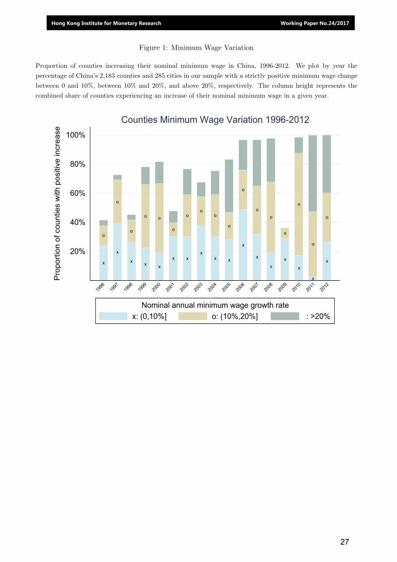
Figure 1: Minimum Wage Variation

Proportion of counties increasing their nominal minimum wage in China, 1996-2012. We plot by year the

percentage of China’s 2,183 counties and 285 cities in our sample with a strictly positive minimum wage change

between 0 and 10%, between 10% and 20%, and above 20%, respectively. The column height represents the

combined share of counties experiencing an increase of their nominal minimum wage in a given year.

x

o

x

o

x

o

x

o

x

o

x

o

x

o

x

o

x

o

x

o

x

o

x

o

x

o

x

o

x

o

x

o

x

o

20%

40%

60%

80%

100%

Pro

porti

on o

f cou

ntie

s w

ith p

ositi

ve in

crea

se

1996

1997

1998

1999

2000

2001

2002

2003

2004

2005

2006

2007

2008

2009

2010

2011

2012

Counties Minimum Wage Variation 1996-2012

x: (0,10%] o: (10%,20%] : >20%Nominal annual minimum wage growth rate

27


Figure 2: Household Consumption and County Minimum Wages I

Average real consumption changes are plotted for minimum wage dependent households (S > 0.5, red crosses)

and those without minimum wage income (S = 0, blue dots). We sort all households into 40 bins according to

the magnitude of the local real minimum wage increase relative to province-level average minimum wages. The

dashed line represents the fitted linear relationship for minimum wage dependent households and the solid line

for households without minimum wage income. The source regression has 32,355 household-level observations.

A standard t-test for the statistical difference of the two slopes produces a t-statistic of 1.56

Corr.: 1.420(0.871)

Corr.: -0.028(0.577)

-100

010

0030

0050

00H

H A

nnua

l Cha

nge

in R

eal C

onsu

mpt

ion

(RM

B)

-500 0 500 1000Real Minimum Wage Residual Change (RMB)

S=0 S>0.5

All Counties

28


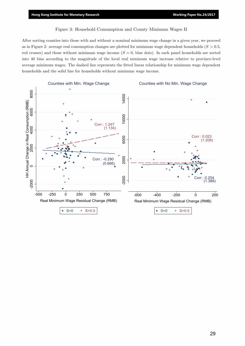
Figure 3: Household Consumption and County Minimum Wages II

After sorting counties into those with and without a nominal minimum wage change in a given year, we proceed

as in Figure 2: average real consumption changes are plotted for minimum wage dependent households (S > 0.5,

red crosses) and those without minimum wage income (S = 0, blue dots). In each panel households are sorted

into 40 bins according to the magnitude of the local real minimum wage increase relative to province-level

average minimum wages. The dashed line represents the fitted linear relationship for minimum wage dependent

households and the solid line for households without minimum wage income.

Corr.: 1.247(1.134)

Corr.: -0.290(0.666)

-200

00

2000

4000

6000

8000

HH

Ann

ual C

hang

e in

Rea

l Con

sum

ptio

n (R

MB)

-500 -250 0 250 500 750

Real Minimum Wage Residual Change (RMB)

S=0 S>0.5

Counties with Min. Wage Change

Corr.: 0.023(1.206)

Corr.: 0.254(1.388)

-200

020

0060

0010

000

1400

0

-600 -400 -200 0 200

Real Minimum Wage Residual Change (RMB)

S=0 S>0.5

Counties with No Min. Wage Change

29


Table 1: Minimum Wage Relative to Median Wage and Minimum Wage Growth

Reported are the average minimum wage bite by year and the annual growth rate of the real minimum wage.

The minimum wage bite is computed as the ratio of the minimum wage (MW) to the median wage in each

county and then averaged across counties. Standard deviations are provided in parentheses below.

Year 2002 2003 2004 2005 2006 2007 2008 2009

MW relative to median wage 0.202 0.201 0.197 0.198 0.201 0.185 0.189 0.176

(0.042) (0.043) (0.046) (0.045) (0.045) (0.045) (0.053) (0.045)

Real MW growth 12.99 7.97 8.71 12.32 7.53 8.74 8.92 8.04

(7.71) (6.24) (8.17) (6.96) (6.83) (8.07) (6.11) (2.61)

Table 2: Persistence of Real Minimum Wage Shock

We regress changes in the real minimum wage (∆MWct) on the lagged real minimum wages (MWct−1)

controlling for trend growth. The regressions add county or province-year fixed effects as specified in Equation

(1) to limit the influence of cross-county spatial dependence. A significant negative coefficient implies

reversion of the minimum wage shocks to trend growth. Standard errors clustered at county level are shown

in parentheses. Stars ∗∗∗, ∗∗, and ∗ indicate statistical significance at the 1, 5, and 10 percent levels, respectively.

Dep. variable: Real minimum wage change, ∆MWc,t

1992-2012 2002-2009

(1) (2) (3) (4) (5) (6) (7) (8)

MWc,t−1 -0.005 0.022 -0.118 -0.119 -0.031 0.023 -0.259 -0.260(0.003) (0.003)*** (0.008)*** (0.009)*** (0.005)*** (0.003)*** (0.011)*** (0.012)***

Trend Yes Yes Yes Yes Yes Yes Yes YesProvince-year FE Yes Yes Yes Yes Yes YesCounty FE Yes YesCounty Trend Yes YesObs. 37320 37320 37320 37320 17464 17464 17464 17464N. clusters 2183 2183 2183 2183 2183 2183 2183 2183R2 0.310 0.862 0.871 0.876 0.011 0.810 0.842 0.852

30


Table 3: Household Income Sources and the Real Minimum Wage

We regress the levels of household real annual labor income in Columns (1)-(3), transfer income in Columns

(4)-(6), and their sum in Column (7)-(9), on the local effective real minimum wage level. The samples consist

of all households for which the labor income share S from wages near the minimum wage represents more than

25% (S > 0.25), or more than 50% (S > 0.5), or more than 75% (S > 0.75) of household labor income. All

regressions include household, county and interacted province-year fixed effects, city level controls and county

time-trends as specified in Equation (7). We report standard errors clustered at county level in parentheses,

two-way clustered at county and city-year level in brackets and two-way clustered at county and province-year

level in curly brackets. Stars ∗∗∗, ∗∗, and ∗ indicate statistical significance at the 1, 5, and 10 percent levels,

respectively

Dep. variables: Household Labor Income Household Transfer Income HH Labor and Transfer Income

MW dependency: S > 0.25 S > 0.5 S > 0.75 S > 0.25 S > 0.5 S > 0.75 S > 0.25 S > 0.5 S > 0.75

(1) (2) (3) (4) (5) (6) (7) (8) (9)

Minimum wage 0.710 1.378 1.563 0.308 0.767 1.091 0.965 2.017 2.475

(0.522) (0.636)∗∗ (0.743)∗∗ (0.209) (0.567) (0.577)∗ (0.581)∗ (0.729)∗∗∗ (0.758)∗∗∗

[0.540) [0.675)∗∗ [0.772]∗∗ [0.217] [0.575] [0.581]∗ [0.600] [0.754]∗∗∗ [0.934]∗∗∗

{0.592} {0.754}∗ {0.895}∗ {0.242} {0.605} {0.683} {0.614} {0.799}∗∗ {0.850}∗∗∗

City level controls Yes Yes Yes Yes Yes Yes Yes Yes Yes

Household FE Yes Yes Yes Yes Yes Yes Yes Yes Yes

County trend Yes Yes Yes Yes Yes Yes Yes Yes Yes

Province × year FE Yes Yes Yes Yes Yes Yes Yes Yes Yes

Observations 14,031 4,267 3,899 14,031 4,267 3,899 14,031 4,267 3,899

Number of clusters 474 336 328 474 336 328 474 336 328

Adjusted R2 0.864 0.889 0.889 0.614 0.606 0.583 0.848 0.870 0.872

31


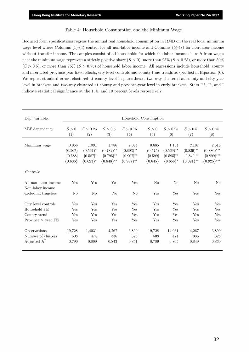
Table 4: Household Consumption and the Minimum Wage

Reduced form specifications regress the annual real household consumption in RMB on the real local minimum

wage level where Columns (1)-(4) control for all non-labor income and Columns (5)-(8) for non-labor income

without transfer income. The samples consist of all households for which the labor income share S from wages

near the minimum wage represent a strictly positive share (S > 0), more than 25% (S > 0.25), or more than 50%

(S > 0.5), or more than 75% (S > 0.75) of household labor income. All regressions include household, county

and interacted province-year fixed effects, city level controls and county time-trends as specified in Equation (6).

We report standard errors clustered at county level in parentheses, two-way clustered at county and city-year

level in brackets and two-way clustered at county and province-year level in curly brackets. Stars ∗∗∗, ∗∗, and ∗

indicate statistical significance at the 1, 5, and 10 percent levels respectively.

Dep. variable: Household Consumption

MW dependency: S > 0 S > 0.25 S > 0.5 S > 0.75 S > 0 S > 0.25 S > 0.5 S > 0.75

(1) (2) (3) (4) (5) (6) (7) (8)

Minimum wage 0.856 1.091 1.786 2.054 0.885 1.184 2.107 2.515

(0.567) (0.561)∗ (0.782)∗∗ (0.893)∗∗ (0.575) (0.569)∗∗ (0.829)∗∗ (0.880)∗∗∗

[0.588] [0.587]∗ [0.795]∗∗ [0.907]∗∗ [0.599] [0.595]∗∗ [0.840]∗∗ [0.899]∗∗∗

{0.636} {0.623}∗ {0.848}∗∗ {0.987}∗∗ {0.645} {0.656}∗ {0.891}∗∗ {0.925}∗∗∗

Controls:

All non-labor income Yes Yes Yes Yes No No No No

Non-labor income

excluding transfers No No No No Yes Yes Yes Yes

City level controls Yes Yes Yes Yes Yes Yes Yes Yes

Household FE Yes Yes Yes Yes Yes Yes Yes Yes

County trend Yes Yes Yes Yes Yes Yes Yes Yes

Province × year FE Yes Yes Yes Yes Yes Yes Yes Yes

Observations 19,728 1,4031 4,267 3,899 19,728 14,031 4,267 3,899

Number of clusters 508 474 336 328 508 474 336 328

Adjusted R2 0.790 0.809 0.843 0.851 0.789 0.805 0.849 0.860

32


Table 5: Household Consumption under Labor Income Shocks

We report 2SLS level regressions in which real annual household consumption in RMB is alternatively regressed

on the household’s fitted annual real labor income level in Columns (1)-(4), or the fitted annual real labor

income plus transfers level in Columns (5)-(8). The first-stage regressions are reported in Table 2. The samples

consist of all households for which the labor income share S from wages near the minimum wage represent

a strictly positive share (S > 0), more than 25% (S > 0.25), or more than 50% (S > 0.5), or more than

75% (S > 0.75) of household labor income. All regressions include city level controls, household fixed effects,

interacted province-year fixed effects, and county time-trends as specified in Equation (8). We report standard

errors clustered at county level in parentheses, two-way clustered at county and city-year level in brackets and

two-way clustered at county and province-year level in curly brackets. The p-values in the last line refer to a

test under the null hypothesis of weak instruments (Kleibergen and Paap, 2006). Stars ∗∗∗, ∗∗, and ∗ indicate

statistical significance at the 1, 5, and 10 percent levels, respectively.

Dep. variable: Household Consumption

MW dependency: S > 0 S > 0.25 S > 0.5 S > 0.75 S > 0 S > 0.25 S > 0.5 S > 0.75

(1) (2) (3) (4) (5) (6) (7) (8)

Fitted labor income 1.687 1.538 1.296 1.314

(1.415) (0.865)∗ (0.609)∗∗ (0.651)∗∗

[1.417] [0.838]∗ [0.603]∗∗ [0.644]∗∗

{1.375} {0.863}∗ {0.572}∗∗ {0.609}∗∗

Fitted labor and

transfer income 1.117 1.227 1.045 1.016

(0.712) (0.555)∗∗ (0.375)∗∗∗ (0.363)∗∗∗

[0.707] [0.539]∗∗ [0.363]∗∗∗ [0.354]∗∗∗

{0.693} {0.522}∗∗ {0.370}∗∗∗ {0.341}∗∗∗

City-level controls Yes Yes Yes Yes Yes Yes Yes Yes

Household FE Yes Yes Yes Yes Yes Yes Yes Yes



Observations 19, 728 14, 031 4, 270 3, 903 19, 728 14, 031 4, 270 3, 903


H0: Weak instruments

(p-value) 0.325 0.209 0.038 0.040 0.182 0.134 0.005 0.002

33


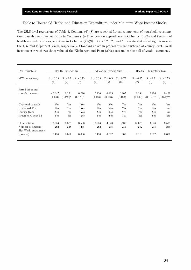
Table 6: Household Health and Education Expenditure under Minimum Wage Income Shocks

The 2SLS level regressions of Table 5, Columns (6)-(8) are repeated for subcomponents of household consump-

tion, namely health expenditure in Columns (1)-(3), education expenditure in Columns (4)-(6) and the sum of

health and education expenditure in Columns (7)-(9). Stars ∗∗∗, ∗∗, and ∗ indicate statistical significance at

the 1, 5, and 10 percent levels, respectively. Standard errors in parenthesis are clustered at county level. Weak

instrument row shows the p-value of the Kleibergen and Paap (2006) test under the null of weak instrument.

Dep. variables: Health Expenditure Education Expenditure Health + Education Exp.

MW dependency S > 0.25 S > 0.5 S > 0.75 S > 0.25 S > 0.5 S > 0.75 S > 0.25 S > 0.5 S > 0.75

(1) (2) (3) (4) (5) (6) (7) (8) (9)

Fitted labor and

transfer income −0.047 0.224 0.226 0.230 0.183 0.205 0.184 0.406 0.431

(0.143) (0.128)∗ (0.120)∗ (0.196) (0.146) (0.133) (0.209) (0.164)∗∗ (0.151)∗∗∗

City-level controls Yes Yes Yes Yes Yes Yes Yes Yes Yes




Observations 12,676 3,876 3,538 12,676 3,876 3,538 12,676 3,876 3,538



(p-value) 0.118 0.017 0.006 0.118 0.017 0.006 0.118 0.017 0.006

34


Table 7: Household Consumption, Minimum Wage Income Shock and Liquidity Constraints

We report 2SLS level regressions in which real annual household consumption is regressed on the household’s

fitted annual real labor and transfer income and on additional interaction terms identifying liquidity constrained

households. The interaction terms are property income dummy in Columns (1)-(3), a capital income dummy

for interest, dividends and insurance income in Columns (4)-(6), and a dummy for (debt-free) house ownership

in Columns (7)-(9). The samples consist of all households for which the labor income share S from wages near

the minimum wage represent a strictly positive share (S > 0), more than 25% (S > 0.25), or more than 50%

(S > 0.5), or more than 75% (S > 0.75) of household labor income. All regressions include city level controls,

household fixed effects, interacted province-year fixed effects, and county time-trends as specified in Equation

(8). We report standard errors clustered at county level in parentheses. The p-values in the last line refer to a

test under the null of weak instruments (Kleibergen and Paap, 2006). Stars ∗∗∗, ∗∗, and ∗ indicate statistical

significance at the 1, 5, and 10 percent levels, respectively.

Dep. variables: Household Consumption

MW dependency S > 0.25 S > 0.5 S > 0.75 S > 0.25 S > 0.5 S > 0.75 S > 0.25 S > 0.5 S > 0.75

(1) (2) (3) (4) (5) (6) (7) (8) (9)

Fitted labor and

transfer income 1.273 1.042 1.012 1.161 0.876 0.921 1.242 1.137 1.135

(0.658)∗ (0.345)∗∗∗ (0.337)∗∗∗ (0.545)∗∗ (0.398)∗∗ (0.380)∗∗ (0.566)∗∗ (0.444)∗∗ (0.428)∗∗∗

Fitted labor and

transfer income −0.062 −0.325 −0.301

× Property income dummy (0.134) (0.164)∗∗ (0.177)∗

Fitted labor and

transfer income −0.042 −0.091 −0.100

× Capital income dummy (0.040) (0.065) (0.070)

Fitted laboe and

transfer income −0.014 −0.075 −0.121

× House owner dummy (0.081) (0.149) (0.148)

City-level controls Yes Yes Yes Yes Yes Yes Yes Yes Yes




Observations 14,031 4,270 3,903 14,031 4,270 3,903 14,031 4,270 3,903



(p-value) 0.176 0.005 0.002 0.147 0.008 0.004 0.139 0.009 0.004

35


Table 8: Household Consumption and Family Structure

We report 2SLS level regressions in which real annual household consumption is regressed on the household’s

fitted annual real labor and transfer income and on additional interaction terms identifying family structure.

The interaction terms are a dummy for one or more children in the household in Columns (1)-(3), an additional

dummy for one or more male children in the household in Columns (4)-(6), or an additional dummy for one or

more male children older than 24 years in Columns (7)-(9). The samples consist of all households for which the

labor income share S from wages near the minimum wage represent a strictly positive share (S > 0), more than

25% (S > 0.25), or more than 50% (S > 0.5), or more than 75% (S > 0.75) of household labor income. All

regressions include city level controls, household fixed effects, interacted province-year fixed effects, and county

time-trends as specified in Equation (8). We report standard errors clustered at county level in parentheses, two-

way clustered at county and city-year level in brackets and two-way clustered at county and province-year level

in curly brackets. The p-values in the last line refer to a test under the null of weak instruments (Kleibergen and

Paap, 2006). Stars ∗∗∗, ∗∗, and ∗ indicate statistical significance at the 1, 5, and 10 percent levels, respectively.

Dep. variables: Household Consumption

MW dependency: S > 0.25 S > 0.5 S > 0.75 S > 0.25 S > 0.5 S > 0.75 S > 0.25 S > 0.5 S > 0.75

(1) (2) (3) (4) (5) (6) (7) (8) (9)

Fitted labor and

transfer income 0.997 0.391 0.313 0.960 0.414 0.340 0.998 0.357 0.269

(0.472)∗∗ (0.448) (0.420) (0.433)∗∗ (0.447) (0.425) (0.473)∗∗ (0.439) (0.408)

Fitted labor and

transfer income 0.258 0.702 0.756 0.219 0.728 0.792 0.260 0.664 0.723

× Dummy children (0.181) (0.307)∗∗ (0.277)∗∗∗ (0.183) (0.353)∗∗ (0.321)∗∗ (0.184) (0.300)∗∗ (0.266)∗∗∗

Fitted labor and

transfer income 0.054 −0.044 −0.057

× Dummy male child (0.101) (0.123) (0.130)

Fitted labor and

transfer income −0.006 0.106 0.107

× Dummy adult male child (0.102) (0.133) (0.144)

City level controls Yes Yes Yes Yes Yes Yes Yes Yes Yes




Observations 14,031 4,270 3,903 14,031 4,270 3,903 14,031 4,270 3,903



(p-value) 0.144 0.005 0.002 0.137 0.004 0.001 0.142 0.006 0.002

36


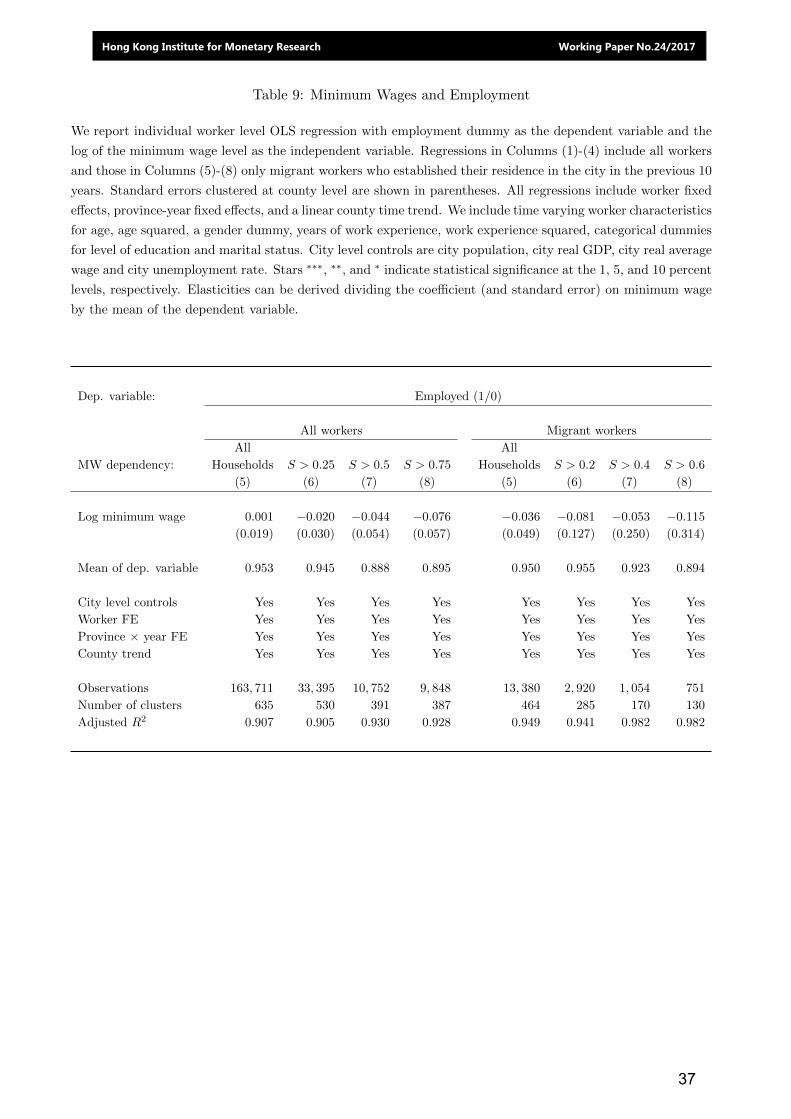
Table 9: Minimum Wages and Employment

We report individual worker level OLS regression with employment dummy as the dependent variable and the

log of the minimum wage level as the independent variable. Regressions in Columns (1)-(4) include all workers

and those in Columns (5)-(8) only migrant workers who established their residence in the city in the previous 10

years. Standard errors clustered at county level are shown in parentheses. All regressions include worker fixed

effects, province-year fixed effects, and a linear county time trend. We include time varying worker characteristics

for age, age squared, a gender dummy, years of work experience, work experience squared, categorical dummies

for level of education and marital status. City level controls are city population, city real GDP, city real average

wage and city unemployment rate. Stars ∗∗∗, ∗∗, and ∗ indicate statistical significance at the 1, 5, and 10 percent

levels, respectively. Elasticities can be derived dividing the coefficient (and standard error) on minimum wage

by the mean of the dependent variable.

Dep. variable: Employed (1/0)

All workers Migrant workers

All All

MW dependency: Households S > 0.25 S > 0.5 S > 0.75 Households S > 0.2 S > 0.4 S > 0.6

(5) (6) (7) (8) (5) (6) (7) (8)

Log minimum wage 0.001 −0.020 −0.044 −0.076 −0.036 −0.081 −0.053 −0.115

(0.019) (0.030) (0.054) (0.057) (0.049) (0.127) (0.250) (0.314)

Mean of dep. variable 0.953 0.945 0.888 0.895 0.950 0.955 0.923 0.894


Worker FE Yes Yes Yes Yes Yes Yes Yes Yes



Observations 163, 711 33, 395 10, 752 9, 848 13, 380 2, 920 1, 054 751


Adjusted R2 0.907 0.905 0.930 0.928 0.949 0.941 0.982 0.982

37


Table 10: Minimum Wages and Occupation Change

We report individual worker level OLS regression where the dependent variable is a dummy for occupation

switching from the previous year (=1 if switch). The exogenous variable is the log of the minimum wage

level. Regressions in Columns (1)-(4) include all workers and those in Columns (5)-(8) only migrant workers.

To increase the number of observations and the power of the estimates we do not restrict the regressions to

recent immigrants. Standard errors clustered at county level are shown in parentheses. All regressions include

worker fixed effects, province-year fixed effects and a linear county time trend. We include time varying worker

characteristics for age, age squared, a gender dummy, years of work experience, work experience squared,

categorical dummies for level of education and marital status. City level controls are city population, city real

GDP, city real average wage and city unemployment rate. Stars ∗∗∗, ∗∗, and ∗ indicate statistical significance

at the 1, 5, and 10 percent levels, respectively. Elasticities can be derived dividing the coefficient (and standard

error) on minimum wage by the mean of the dependent variable.

Dep. variable: Occupation switch (1/0)

All workers Migrant workers

All All

MW dependency: Households S > 0.25 S > 0.5 S > 0.75 Households S > 0.2 S > 0.4 S > 0.6

(5) (6) (7) (8) (5) (6) (7) (8)

Log minimum wage 0.067 0.069 0.066 0.208 0.059 0.125 0.357 0.656

(0.120) (0.196) (0.283) (0.270) (0.109) (0.334) (0.459) (0.633)

Mean of dependent variable 0.079 0.089 0.092 0.088 0.080 0.092 0.095 0.094


Worker FE Yes Yes Yes Yes Yes Yes Yes Yes



Observations 50, 184 9, 714 2, 746 2, 514 20, 811 4, 110 1, 359 862


Adjusted R2 0.603 0.621 0.671 0.683 0.652 0.700 0.780 0.820

38


Appendix A: Predicting the Minimum Wage

For the correct interpretation of econometric estimates, it is important that minimum wage changes in China are

non-predictable and can be considered as a random income shocks from the perspective of households. In this

section we show that wage changes are indeed non-unpredictable even when using rich information sets with

socio-economic and political data typically beyond the reach of individual households.

First, we use county-level socio-economic data to explore the predictability of minimum wage

changes. Second, we aggregate the Urban Household Survey (UHS) data and examine whether these

alternative county-level aggregates show any predictability for the minimum wage change. Third, we use

biographical data on the two most important political decision makers in Chinese counties, namely the

mayor and party secretary, to predict minimum wage changes. Throughout this exercise, we code any

nominal minimum wage change in a county as a binary (0/1) decision. But the results are robust if the

(level) change of the minimum wage becomes the dependent variable.

A.1. Predictability Based on County-Level Data

Table A1 presents OLS regression based on country-level socio-economic data to examine the pre-

dictability of minimum wage changes codes as binary outcomes (0/1). The socio-economic data are sourced

from the Prefecture Statistical Annual Yearbooks, the Fiscal Statistics for Prefectures, Mu-nicipalities and

Counties and the National Demographic Yearbook. We note that these county level data have an imperfect

overlap with the sample of counties in our main data and so we do not use them in the analysis on

household consumption. Yet they are still a useful data source for a test of predictability of the minimum

wage change.

Columns (1)-(3) include the listed covariates as contemporaneous changes and Columns (4)-(6) as lagged changes.

All variables are expressed in real terms using a province-level consumer price deflator. We find that none of the

county variables robustly predicts (either as contemporaneous or lagged changes) minimum wage across

specifications. In Column (3) only the average salary in the county shows weak negative relation with the decision

to change the minimum wage. But this marginal significance disappears when we use two-way clustering at the

county and province-year levels (not shown). Overall, we conclude that the results indicate no systematic

relationship between county-level socio-economic variables and minimum wage changes.

A.2. Predictability Based on Aggregates of Household Survey Data

Table A2 explores the predictability of minimum wage changes based on county-level aggregates of the Urban

Household Survey (UHS) used throughout the paper. The set of counties covered differs from Table A1 and the

time span is restricted to the period 2002-2009. The county-level aggregates of the UHS data are complimented by

city-level variables drawn from the China City Statistical Yearbooks in the Chinese Statistical Yearbook Database

(CNKI). Again, no statistically significant relationship appears between the various covariates and the minimum

wage change. The results also holds if we consider level change in minimum wages as an alternative dependent

variable.

A.3. Predictability Based on Biographical Data of Local Political Leaders

In democratic societies, important political decisions like minimum wage changes are subject to open political

debate and depend on the parliamentary strength of competing political parties. Chinese

39


politics represents an entirely different political setting, important policy issues can be contingent on the

preferences of the key local decision makers, Yao and Zhang (2015). Minimum wage changes in China originate inan administrative and political process that is not subject to a open debate that involves the public at large. This

implies that little public information is generated that would allow households to anticipate minimum wage

changes. Moreover, the timing of minimum wage changes is highly discretionary across regions and the law only

stipulates the requirement of regular review, not a mandatory change. While individual policy preferences are

hard to observe, such preferences and policy outcomes could nevertheless be related to personal political career

paths and curricula or to demographic characteristics of local leaders.

The two main political actors in Chinese local politics are the mayor, appointed by the local communist party

assembly, and the local party secretary, appointed by personal office of the cen-tral party administration. Their

biographical data are available in the Chinese Bureaucracies and Leaders Database, which is constructed and

maintained by the National Chengchi University.28 We use biographical information about their respective tenure, their first year in office, the their year of promotion and retirement, as well as their age and experience.

Table A3 presents the regression re-sults with seven biographical variables for the local party secretary and an

equal number for the local mayor. Yet none of these biographical variables has any predictive value for minimum

wage change. Similar results are obtained if we define the dependent variable as first difference in minimum wage

levels.

Overall, we conclude from Tables A1, A2 and A3 that minimum wage changes in China are not

predictable based on county-level socio-economic data or even biographical data on the two most powerful

local politicians.

28 See http://ics.nccu.edu.tw/chinaleaders/. The data are documented in Shih et al. (2010), Yao and Zhang (2015) and Zhou (2016).

40


Table A1: County-Level Determinants of Minimum Wage Changes, 1997-2010

The minimum wage change as the dependent variable is coded as a binary decision outcome (1/0)with 1 representing a change and regressed on various county-level socio-economic variables. Columns(1)-(3) use covariates in first differences contemporaneous with the minimum wage change; Columns(4)-(6) use covariates in first differences lagged by one year relative to the minimum wage change.Standard errors are clustered at county level are shown in parentheses. Stars indicate significancelevels at p-values: * p < 0.1, ** p < 0.05, *** p < 0.01.

Dep. variable: Minimum wage change dummy (1/0)

Covariates in ∆t Covariates in ∆t−1

(1) (2) (3) (4) (5) (6)

Ln(County Real GDP) -0.042 -0.191*** -0.005 -0.076*** -0.097** -0.012(0.035) (0.045) (0.010) (0.028) (0.049) (0.009)

Ln(County Population) -0.077 -0.240* 0.005 0.165 0.176 0.012(0.103) (0.128) (0.009) (0.101) (0.153) (0.010)

Ln(County Total Employment) -0.014 -0.011 -0.001 0.004 0.007 -0.000(0.014) (0.016) (0.001) (0.016) (0.023) (0.001)

County Government Balance/GDP -0.001** -0.001 -0.000 -0.000 -0.000 0.000(0.001) (0.001) (0.000) (0.001) (0.001) (0.000)

Ln(County Salary per capita) 0.016 0.002 -0.020* 0.021*** 0.006 0.002(0.013) (0.013) (0.011) (0.007) (0.007) (0.001)

Ln(County Employment in Agriculture) -0.021** -0.016 0.000 0.026*** 0.030** 0.001(0.009) (0.010) (0.001) (0.009) (0.012) (0.001)

Ln(Real County Savings) -0.002 -0.007 -0.002 0.014 0.005 0.001(0.015) (0.016) (0.002) (0.013) (0.019) (0.001)

County FE Yes Yes Yes Yes Yes YesYear FE Yes YesCounty Trend Yes Yes Yes YesProvince-year FE Yes YesObservations 8716 8716 8714 7139 7139 7137Number of clusters 1651 1651 1651 1647 1647 1647Adjusted R-square 0.591 0.697 0.990 0.625 0.686 0.992

41


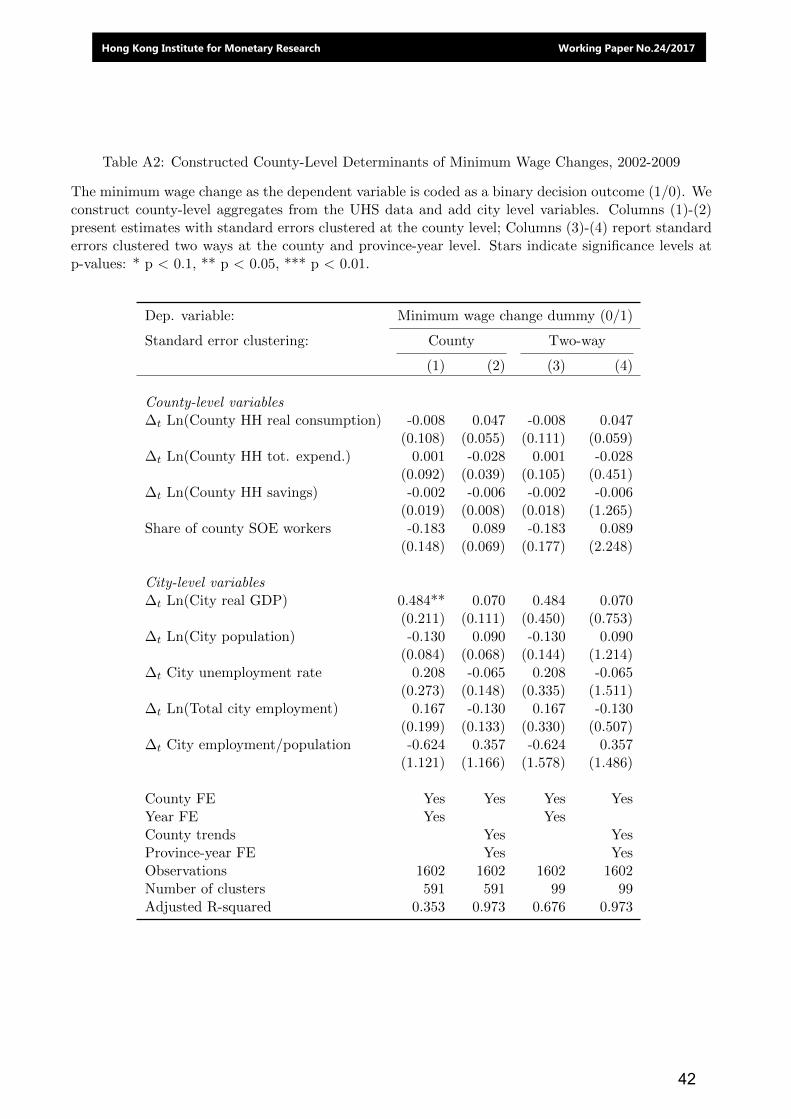
Table A2: Constructed County-Level Determinants of Minimum Wage Changes, 2002-2009

The minimum wage change as the dependent variable is coded as a binary decision outcome (1/0). Weconstruct county-level aggregates from the UHS data and add city level variables. Columns (1)-(2)present estimates with standard errors clustered at the county level; Columns (3)-(4) report standarderrors clustered two ways at the county and province-year level. Stars indicate significance levels atp-values: * p < 0.1, ** p < 0.05, *** p < 0.01.


Standard error clustering: County Two-way

(1) (2) (3) (4)

County-level variables∆t Ln(County HH real consumption) -0.008 0.047 -0.008 0.047

(0.108) (0.055) (0.111) (0.059)∆t Ln(County HH tot. expend.) 0.001 -0.028 0.001 -0.028

(0.092) (0.039) (0.105) (0.451)∆t Ln(County HH savings) -0.002 -0.006 -0.002 -0.006

(0.019) (0.008) (0.018) (1.265)Share of county SOE workers -0.183 0.089 -0.183 0.089

(0.148) (0.069) (0.177) (2.248)

City-level variables∆t Ln(City real GDP) 0.484** 0.070 0.484 0.070

(0.211) (0.111) (0.450) (0.753)∆t Ln(City population) -0.130 0.090 -0.130 0.090

(0.084) (0.068) (0.144) (1.214)∆t City unemployment rate 0.208 -0.065 0.208 -0.065

(0.273) (0.148) (0.335) (1.511)∆t Ln(Total city employment) 0.167 -0.130 0.167 -0.130

(0.199) (0.133) (0.330) (0.507)∆t City employment/population -0.624 0.357 -0.624 0.357

(1.121) (1.166) (1.578) (1.486)

County FE Yes Yes Yes YesYear FE Yes YesCounty trends Yes YesProvince-year FE Yes YesObservations 1602 1602 1602 1602Number of clusters 591 591 99 99Adjusted R-squared 0.353 0.973 0.676 0.973

42


Table A3: Political Characteristics and Minimum Wage Changes, 1997-2010

The minimum wage change as the dependent variable is coded as a binary decision outcome (1/0)with 1 representing a change and regressed on the characteristics of thr local party secretary andthe mayor. Columns (1)-(2) present estimates with standard errors clustered at the county level;Columns (3)-(4) report standard errors clustered two ways at the county and province-year level.Stars indicate significance levels at p-values: * p < 0.1, ** p < 0.05, *** p < 0.01.


Standard error clustering County Two–way

(1) (2) (3) (4)

Party secretary characteristics:First year in office dummy 0.018* 0.004 0.018* 0.004

(0.009) (0.004) (0.009) (0.004)Promotion year dummy 0.049* -0.005 0.049* -0.005

(0.026) (0.007) (0.026) (0.010)Retirement year dummy 0.079** 0.028** 0.079** 0.028

(0.034) (0.013) (0.034) (0.017)Age 0.047 0.018 0.047 0.018

(0.057) (0.016) (0.055) (0.028)Age2 -0.000 -0.000 -0.000 -0.000

(0.001) (0.000) (0.001) (0.000)Province experience dummy -0.016 0.005 -0.016 0.005

(0.030) (0.009) (0.030) (0.009)City tenure length (years) 0.007 0.004 0.007 0.004

(0.007) (0.003) (0.007) (0.003)Mayor characteristics:First year in office dummy 0.090 -0.008 0.090 -0.008

(0.091) (0.026) (0.085) (0.026)Promotion year dummy 0.030 -0.001 0.030 -0.001

(0.023) (0.005) (0.025) (0.007)Retirement year dummy -0.016 -0.001 -0.016 -0.001

(0.043) (0.013) (0.043) (0.018)Age -0.003 0.006 -0.003 0.006

(0.052) (0.017) (0.063) (0.018)Age2 0.000 -0.000 0.000 -0.000

(0.001) (0.000) (0.001) (0.000)Province experience dummy 0.024 0.003 0.024 0.003

(0.023) (0.006) (0.026) (0.008)City tenure length (years) 0.090 -0.007 0.090 -0.007

(0.091) (0.025) (0.084) (0.025)

County FE Yes Yes Yes YesYear FE Yes YesCounty Trend Yes YesProvince-year FE Yes YesObservations 14548 14544 14548 14544Number of clusters 258 257 232 228Adjusted R-square 0.383 0.964 0.383 0.964

43


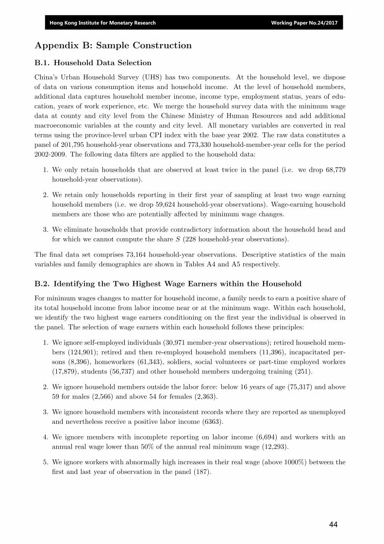
Appendix B: Sample Construction

B.1. Household Data Selection

China’s Urban Household Survey (UHS) has two components. At the household level, we dispose

of data on various consumption items and household income. At the level of household members,

additional data captures household member income, income type, employment status, years of edu-

cation, years of work experience, etc. We merge the household survey data with the minimum wage

data at county and city level from the Chinese Ministry of Human Resources and add additional

macroeconomic variables at the county and city level. All monetary variables are converted in real

terms using the province-level urban CPI index with the base year 2002. The raw data constitutes a

panel of 201,795 household-year observations and 773,330 household-member-year cells for the period

2002-2009. The following data filters are applied to the household data:

1. We only retain households that are observed at least twice in the panel (i.e. we drop 68,779

household-year observations).

2. We retain only households reporting in their first year of sampling at least two wage earning

household members (i.e. we drop 59,624 household-year observations). Wage-earning household

members are those who are potentially affected by minimum wage changes.

3. We eliminate households that provide contradictory information about the household head and

for which we cannot compute the share S (228 household-year observations).

The final data set comprises 73,164 household-year observations. Descriptive statistics of the main

variables and family demographics are shown in Tables A4 and A5 respectively.

B.2. Identifying the Two Highest Wage Earners within the Household

For minimum wages changes to matter for household income, a family needs to earn a positive share of

its total household income from labor income near or at the minimum wage. Within each household,

we identify the two highest wage earners conditioning on the first year the individual is observed in

the panel. The selection of wage earners within each household follows these principles:

1. We ignore self-employed individuals (30,971 member-year observations); retired household mem-

bers (124,901); retired and then re-employed household members (11,396), incapacitated per-

sons (8,396), homeworkers (61,343), soldiers, social volunteers or part-time employed workers

(17,879), students (56,737) and other household members undergoing training (251).

2. We ignore household members outside the labor force: below 16 years of age (75,317) and above

59 for males (2,566) and above 54 for females (2,363).

3. We ignore household members with inconsistent records where they are reported as unemployed

and nevertheless receive a positive labor income (6363).

4. We ignore members with incomplete reporting on labor income (6,694) and workers with an

annual real wage lower than 50% of the annual real minimum wage (12,293).

5. We ignore workers with abnormally high increases in their real wage (above 1000%) between the

first and last year of observation in the panel (187).

44


6. We ignore household members with inconsistent age records that increase by more than one from

one year to another or decrease (6,553) and household members who are not relatives (210).

The two highest wage earners within the household are in most cases (80.5%) the head of the

household and the spouse. We retain for the household-level regressions their wage income, age,

gender, level of education and years of work experience, years since migration to the city, marital

status, industry and occupation.

B.3. Minimum Wage Dependency of a Household

Finally, we define the share S of household income coming from the wage income (of the two highest

wage earners) at or near the minimum wage. We consider a wage earner to earn a minimum wage

if her salary ranges between 50% and 150% of the real minimum wage of their county of residence

in the first year the individual is observed in the panel. Conditioning on the first year of household

observation assures that the treated household group remains unchanged over time.

Among the two highest wage earners of all retained households, we identify 32,580 (18.72%) treated

(minimum wage) and 141,442 (81.28 percent) non-treated worker-year observations. We also under-

take extensive robustness checks with respect to a narrower salary range from 50% to 120% of the

local minimum wage, which results in 18,721 (10.76%) and 155,301 (89.24%) non-treated worker-year

observations, respectively.

Table A4 reports summary statistics on the households income and expenditure components for

household groups sorted by their minimum wage income share S. Column (1) includes all households,

Column (2) with S = 0 all households without wage income at or near the minimum wage, whereas

Columns (3)-(5) feature household groups of increasing minimum wage dependency.

45


Table A4: Incomes and Expenditures Share of Disposable Income

The table summarize the household income and expenditure components as a share of disposableincome by different household types sorted by their share S of minimum wage income in total householdincome. Data are from the Urban Household Survey (UHS) and cover the period from 2002 to 2009.Reported are average values for the entire period and standard errors are in parentheses below.

MW dependency: All S=0 S>0 S>0.5 S>0.75Households

Income components:Labor income 0.902 0.917 0.862 0.779 0.792

(0.158) (0.140) (0.192) (0.243) (0.242)Transfer income 0.083 0.069 0.120 0.195 0.185

(0.146) (0.128) (0.181) (0.234) (0.233)Transfer income net of pension 0.041 0.035 0.055 0.082 0.068

(0.081) (0.071) (0.100) (0.124) (0.106)

Expenditure components:Consumption 0.724 0.705 0.773 0.820 0.817

(0.311) (0.310) (0.308) (0.359) (0.364)Housing expenditure 0.055 0.060 0.040 0.035 0.031

(0.491) (0.502) (0.458) (0.441) (0.420)Education expenditure 0.112 0.112 0.111 0.103 0.102

(0.125) (0.119) (0.139) (0.154) (0.155)Health expenditure 0.043 0.041 0.048 0.054 0.053

(0.084) (0.075) (0.105) (0.116) (0.117)Durables expenditure 0.039 0.041 0.036 0.032 0.032

(0.060) (0.063) (0.051) (0.042) (0.042)Savings 0.240 0.264 0.179 0.143 0.146

(0.309) (0.324) (0.254) (0.228) (0.232)

Observations 73164 53054 20110 4365 3990Share of observations in sample 0.72 0.27 0.06 0.05Share of total labor income 0.819 0.181 0.026 0.024

46


Table A5: Household Demographics

The table summarize the household demographics by household type sorted on the share S of minimumwage earnings in total household income. Data are from the Urban Household Survey (UHS) and coverthe period 2002-2009. Reported are average values for the entire period and standard errors are inparentheses below. Family head refers to the household member with the highest labor income; SOEstands for State Owned Enterprise; education is a categorical variable with a total of nine categories:no schooling, basic literacy classes, primary school, junior high school, senior middle school, secondary,college enrollment, bachelor completed, graduated.

MW dependency: All S=0 S>0 S>0.5 S>0.75Households

Family size 3.145 3.118 3.215 3.345 3.355(0.724) (0.703) (0.773) (0.862) (0.869)

House ownership 0.870 0.890 0.818 0.778 0.776(0.336) (0.313) (0.386) (0.415) (0.417)

Years since migrating 8.047 8.429 7.040 6.047 6.149(11.10) (11.15) (10.91) (10.63) (10.69)

SOE employee share 0.735 0.778 0.620 0.436 0.441(0.441) (0.415) (0.485) (0.496) (0.497)

Female Head 0.270 0.292 0.211 0.318 0.316(0.444) (0.455) (0.408) (0.466) (0.465)

Age of the family head 41.38 41.29 41.62 40.58 40.47(7.842) (7.742) (8.095) (8.686) (8.754)

Family head education 5.914 6.127 5.351 4.929 4.941(1.441) (1.419) (1.345) (1.172) (1.174)

Head work experience (years) 20.87 20.84 20.95 19.35 19.23(8.703) (8.590) (8.995) (9.804) (9.859)

Observations 73164 53054 20110 4365 3990

47


Appendix C: Specification Issues

Table A6: Alternative First-Stage Regressions

Household annual real labor income is regressed on the annual real minimum wage for households sorted by

the share S of household minimum wage income in total income under two alternative specifications. Columns

(1)-(4) do not include linear county time trends and province-year fixed effects in the specification, while

Columns (5)-(8) control for linear county time trends and province-year fixed effects. We report standard

errors clustered at county level in parentheses, two way clustered errors at county and city-year level in

brackets and two-way clustered errors at county and province-year level in curly brackets. Stars indicate

significance levels at the following p-values: * p < 0.1, ** p < 0.05, *** p < 0.01. All regressions include

controls for the two highest labor income earners in the household, namely age and age squared, a gender

dummy, years of work experience and work experience squared, years since migration to the city and squared,

family size as measured by the number of family members and a house ownership dummy. Additional categor-

ical control variables characterize the level of education, marital status, industry and occupation. City-level

variation is accounted for by city population, city real GDP, city real average wage and city unemployment rate.

Dep. variable: Household Real Labor Income

Household FE and year FE County trends and province-year FE

MW dependency: S = 0 S > 0 S > 0.5 S > 0.75 S = 0 S > 0 S > 0.5 S > 0.75(1) (2) (3) (4) (5) (6) (7) (8)

Real MinimumWage (in RMB) 1.222 1.832 2.161 1.976 0.012 0.507 1.378 1.563

(0.296)*** (0.388)*** (0.562)*** (0.568)*** (0.524) (0.473) (0.636)** (0.743)**[0.316]*** [0.547]*** [0.618]*** [0.639]*** [0.521] [0.497] [0.660]** [0.771]**{0.386}*** {0.526}*** {0.829}** {0.833}** {0.570} {0.496} {0.750}* {0.878}*

Observations 51,330 19,728 4,270 3,903 51,330 19,728 4,267 3899Number of clusters 600 508 336 328 600 508 336 328Adjusted R-square 0.925 0.861 0.820 0.821 0.930 0.883 0.889 0.889

Household FE Yes Yes Yes Yes Yes Yes Yes YesYear FE Yes Yes Yes YesCounty trends Yes Yes Yes YesProvince-year FE Yes Yes Yes Yes

48


Appendix D: OLS Estimates of the Income Elasticity of Consumption

Table A7: OLS Estimates of the Income Elasticity of Consumption

We report OLS regressions, where Columns (1)-(4) estimate the income elasticity of consumption using house-

hold real labor income as the main regressor of interest, whereas Columns (5)-(6) use the sum of labor and

transfer incomes as the main regressor of interest. We report standard errors clustered at county level in

parentheses, two-way clustered errors at the county and city-year level in brackets, and two way clustered

errors at the county and province-year level in curly brackets. Stars indicate significance levels at the fol-

lowing p-values: * p < 0.1, ** p < 0.05, *** p < 0.01. All regressions include controls for the two high-

est labor income earners in the household, namely age and age squared, a gender dummy, years of work

experience and work experience squared, years since migration to the city and squared, family size as mea-

sured by the number of family members and a house ownership dummy. Additional categorical control

variables characterize the level of education, marital status, industry and occupation. City-level variation

is accounted for by city population, city real GDP, city real average wage and city unemployment rate.

Dep. variable: Annual Real Household Consumption


Household reallabor income 0.398 0.439 0.405 0.387

(0.039)*** (0.020)*** (0.082)*** (0.081)***[0.040]*** [0.020]*** [0.083]*** [0.081]***{0.041}*** {0.025}*** {0.089}*** {0.088}***

Household reallabor and transfer 0.388 0.437 0.359 0.334income (0.031)*** (0.023)*** (0.076)*** (0.079)***

[0.031]*** [0.024]*** [0.077]*** [0.080]***{0.032}*** {0.025}*** {0.077}*** {0.081}***

Observations 19,728 14,031 4,267 3,899 19,728 14,031 4,267 3,899Number of clusters 508 474 336 328 508 474 336 328Adjusted R-square 0.809 0.836 0.862 0.868 0.812 0.838 0.868 0.876

Household FE Yes Yes Yes Yes Yes Yes Yes YesCounty trends Yes Yes Yes Yes Yes Yes Yes YesProvince-year FE Yes Yes Yes Yes Yes Yes Yes Yes

49


Appendix E: Parallel Trends and Anticipation Effects

Table A8: Reduced Form Estimates for Augmented Specification

Reduced form specifications regress the annual real household consumption in RMB on the contempora-

neous real local minimum wage level and alternatively lags of one and two years in Columns (1)-(4) and

leads of one and two years in Columns (5)-(8). The samples consist of all households for which the la-

bor income share S from wages near the minimum wage represent a strictly positive share (S > 0), more

than 25% (S > 0.25), or more than 50% (S > 0.5), or more than 75% (S > 0.75) of household labor in-

come. All regressions include household, county and interacted province-year fixed effects. We control for

all other type of income including transfers, we add city level controls, and county time trends as speci-

fied in Equation (9). We report standard errors clustered at county level in parentheses, two-way clustered

at county and city-year level in brackets and two-way clustered at county and province-year level in curly

brackets. Stars ∗∗∗, ∗∗, and ∗ indicate statistical significance at the 1, 5, and 10 percent levels respectively.

Dep. variable: Annual Real Household Consumption

Delayed Income Effects Anticipated Income Effects


Minimum wage 0.989 1.459 2.349 2.523 1.002 0.991 1.398 1.663(0.628) (0.619)** (0.935)** (1.071)** (0.675) (0.684) (0.722)* (0.812)**

Minimum waget−1 -0.619 -0.458 -1.245 -1.212(0.524) (0.597) (1.018) (1.076)

Minimum waget−2 -0.136 0.704 0.802 0.616(0.686) (0.689) (1.391) (1.443)

Minimum waget+1 0.218 -0.098 -0.743 -0.785(0.527) (0.461) (0.801) (0.849)

Minimum waget+2 0.034 -0.100 0.065 0.056(0.549) (0.322) (0.460) (0.585)

HH FE Yes Yes Yes Yes Yes Yes Yes YesCounty Trend Yes Yes Yes Yes Yes Yes Yes YesProvince-year FE Yes Yes Yes Yes Yes Yes Yes Yes

Observations 19,728 14,031 4,265 3,897 19,728 14,031 4,265 3,897Number of clusters 508 474 335 327 508 474 335 327Adjusted R-square 0.790 0.809 0.843 0.851 0.790 0.809 0.843 0.851

50


Documents

HONG KONG INSTITUTE FOR MONETARY … Hong Kong Institute for Monetary Research, its Council of Advisers, or the Board of Directors. Acknowledgments: We thank Jean-Louis Arcand, Marius