Hop-distance based addressing and routing for dense sensor

Ad Hoc Networks 5 (2007) 486–503

www.elsevier.com/locate/adhoc

Hop-distance based addressing and routing for densesensor networks without location information

Serdar Vural *, Eylem Ekici

Department of Electrical and Computer Engineering, The Ohio State University, 2015 Neil Avenue,

205 Dreese Lab., Columbus, OH 43210, United States

Received 1 October 2005; accepted 30 January 2006Available online 6 April 2006

Abstract

One of the most challenging problems in wireless sensor networks is the design of scalable and efficient routing algo-rithms without location information. The use of specialized hardware and/or infrastructure support for localization iscostly and in many deployment scenarios infeasible. In this study, the wave mapping coordinate (WMC) system to addressthe localization problem is introduced for dense sensor networks and a highly efficient routing algorithm applicable toWMC systems is proposed. The performance of the WMC system is evaluated through simulations and compared withthe performance of geographic routing without location information (GWL). The WMC system is found to be highly scal-able and efficient with a simple system set-up procedure. Simulation studies confirm the high routing performance of WMCsystems which is comparable to the performance of greedy geographic routing with the availability of location information.� 2006 Elsevier B.V. All rights reserved.

Keywords: Sensor networks; Routing; Localization

1. Introduction

Wireless sensor networks (WSN), with the avail-ability of small and inexpensive sensing devices thatcan be produced in large numbers, have a wide rangeof application areas. These applications include, butare not limited to, environmental monitoring, real-time data collection in diverse environments, moni-toring complex machinery and processes, querybased applications, distributed surveillance applica-

1570-8705/$ - see front matter � 2006 Elsevier B.V. All rights reserved

doi:10.1016/j.adhoc.2006.01.004

* Corresponding author. Tel.: +1 614 487 9567.E-mail addresses: [email protected] (S. Vural), ekici@ece.

osu.edu (E. Ekici).

tions, habitat monitoring, and intelligent transporta-tion systems. Due to the wide range of applicationareas of WSNs, research efforts to enhance the com-munication capability and quality of sensor networkshas been growing over the last five years.

One of the major research topics for WSNs is thedesign of simple, efficient, and scalable routing algo-rithms. One such approach is the geographic routing

[1–3] where geographic locations of sensors are usedfor making routing decisions. In greedy geographic

routing [4], a node forwards packets to a neighbor-ing node whose distance metric to the destinationis the smallest. The distance metric is usually chosenas the geographic distance which is computed using

.

mailto:[email protected]

mailto:ekici@ece. osu.edu

mailto:ekici@ece. osu.edu

S. Vural, E. Ekici / Ad Hoc Networks 5 (2007) 486–503 487

node coordinates. In addition to the distinct advan-tages like simplicity and topology independence,geographic routing algorithms have also disadvan-tages: Geographic routing requires location infor-mation in every sensor node, which poses a rigidrestriction on its usage since such information maynot be available in many deployment scenarios.

Highly accurate localization can be achievedthrough the availability of a GPS device in each sen-sor node [5]. However, fast depletion of sensorenergy sources and increased sensor costs arise astwo major problems. Therefore, many schemes suchas [6–8] propose to compute sensor locations with-out the use of GPS. Nonetheless, these solutionsare based on reference infrastructures and the com-plexity of sensor nodes is increased with therequired additional hardware. Due to these reasons,accurate location information is costly to obtain.

Routing in sensor networks without the avail-ability of location information of sensors is a chal-lenging task. Some recent methods aim to adaptgeographic routing to environments without thelocation information of sensor nodes [9,10]. In [9],only a group of sensors do not know their coordi-nates while most others do. Hence, the problem of‘‘lack of location information’’ is not fully takeninto account in [9]. The geographic routing withoutlocation information (GWL) scheme in [10] usesneighborhood information to achieve localizationwithout any reference infrastructure. GWL createsvirtual coordinates of the sensors according to theirneighborhood information. Then, routing is per-formed greedily using these virtual sensor coordi-nates. However, a large number of packetexchanges required by this solution incurs a highoverhead. Furthermore, each sensor node needs torun complex optimization algorithms, increasingthe sensor hardware complexity. Hence, althoughvirtual coordinates of sensors represent a reason-ably useful location information, the GWL schemeremains a complex solution, which is not desirablefor WSNs.

In this study, the wave mapping coordinate

(WMC) system and a highly efficient routing schemespecifically designed for WMC systems is proposed.WMC systems provide approximate localizationwhen no location information is available in densesensor networks. Furthermore, neither special hard-ware nor infrastructure support is required. It isfound that WMC system makes it possible to effi-ciently and easily perform routing of packets. Theperformance of routing in WMC systems is tested

for various node density and sensor field size values.The results are compared with those obtained bygreedy geographic routing (GGR) with the avail-ability of location information. It is observed thatour new routing scheme is highly efficient in termsof packet delivery and path length. The perfor-mance of routing in WMC systems is also comparedwith the GWL method proposed in [10]. It is foundthat the routing scheme in WMC is superior toGWL both in terms of packet delivery performanceand simplicity.

2. Wave mapping coordinate (WMC) system

2.1. Properties of sensors and assumptions

The sensing applications in this study areassumed to require dense and spatially random sen-sor network deployments. Neither complex hard-ware nor signal processing capability is envisionedfor sensors. Sensors have very limited, if any, mobil-ity and they do not necessarily have time synchroni-zation. Furthermore, nodes have identical wirelesscommunication capabilities.

One of the major aspects of the WMC system isthat there are no specific nodes in the network thatcarry special properties. For instance, high-capacitysensors or beacons that have GPS hardware are notutilized. Due to the simplicity of sensor nodes andas the node functionality is kept at a minimum, suchsystems can be deployed densely at low costs. Thehigh number of sensors in turn helps to gain moreaccurate sensing, higher robustness, and better cov-erage of the sensing area.

2.2. The WMC system

The WMC system was initially introduced in [11].The construction of the sensor network coordinatesystem is based on the hop distances of sensor nodesto two designated sensors called wave sources. Thenodes with the same pair of hop distances to thewave sources form groups as explained in Section2.2.1. Hence, a pair of hop distances, one to the firstsource and the other to the second source, is suffi-cient to define a particular group. A third hop dis-tance, hence a third wave source, can be used butis not necessary since an address ambiguity can beeliminated easily by the use of these two wavesources, as explained in Section 2.2.1. Therefore,the use of more than two wave sources in a twodimensional sensor network is unnecessary.

488 S. Vural, E. Ekici / Ad Hoc Networks 5 (2007) 486–503

The system set-up of WMC systems is performedin two stages:

• Network-wide broadcasting stage.• Group-wide broadcasting stage.

WS1 WS2

G5,8

G5,8

Fig. 1. A WMC group.

2.2.1. Network-wide broadcasting stage

The WMC system is based on grouping of sensornodes according to their hop distances to two wavesources.

Definition. Hop distance to WS: The least numberof hops that a packet sent by a WS traverses toreach a particular node.

The Network-wide broadcasting stage, which isthe first stage of the set-up of a WMC system, is per-formed for this grouping purpose. Since there are twowave sources, every sensor node has two hop distancevalues, one for each of the two wave sources. Thesehop distances are regarded as the identification num-bers for sensors. Hence, the pair of hop distances of anode is called the ID-pair of the node. Sensors havingidentical ID-pairs are in the same WMC group.

Definition. WMC group Gi, j: Group of sensorswhose hop distances to the first and second wavesources are i and j, respectively. These nodes allhave the ID-pair ij.

To determine the hop distances of network sen-sor nodes to the wave sources, each of the wavesources broadcast a packet to the network.

Definition. The hop counter: The hop counter field ina broadcast packet is used to keep track of thenumber of hops that the packet has traveled so far.This field is incremented every time the packet isrebroadcast by a node.

Every node in the network keeps track of the hopcounters of the packets they receive. Upon receivinga packet originating from a particular wave source, anode checks the packet’s hop counter to determinewhether its value is less than those of the previouslyreceived packets from the same wave source. As aresult of such updates of hop counters at nodes, allnodes determine the hop distances to the wavesources, and hence their ID-pairs, at the end of thenetwork-wide broadcasting stage.

Definition. Region: The locality where a group ofsensors with identical ID-pairs are found. Forinstance, the area where the sensor nodes of thegroup Gi, j are located is a region.

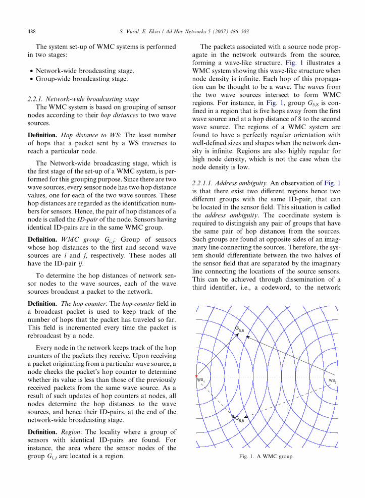
The packets associated with a source node prop-agate in the network outwards from the source,forming a wave-like structure. Fig. 1 illustrates aWMC system showing this wave-like structure whennode density is infinite. Each hop of this propaga-tion can be thought to be a wave. The waves fromthe two wave sources intersect to form WMCregions. For instance, in Fig. 1, group G5,8 is con-fined in a region that is five hops away from the firstwave source and at a hop distance of 8 to the secondwave source. The regions of a WMC system arefound to have a perfectly regular orientation withwell-defined sizes and shapes when the network den-sity is infinite. Regions are also highly regular forhigh node density, which is not the case when thenode density is low.

2.2.1.1. Address ambiguity. An observation of Fig. 1is that there exist two different regions hence twodifferent groups with the same ID-pair, that canbe located in the sensor field. This situation is calledthe address ambiguity. The coordinate system isrequired to distinguish any pair of groups that havethe same pair of hop distances from the sources.Such groups are found at opposite sides of an imag-inary line connecting the sources. Therefore, the sys-tem should differentiate between the two halves ofthe sensor field that are separated by the imaginaryline connecting the locations of the source sensors.This can be achieved through dissemination of athird identifier, i.e., a codeword, to the network


such that the identifiers of the two halves are differ-ent. This identifier can be sent by the groups wherethe wave sources are located. A codeword sent toone side should be blocked so that it is not diffusedto the other side. This is achieved by the groups thatare located on the imaginary line connecting thewave sources. Such groups are called borderline

groups. The details of address ambiguity elimina-tion can be found in [11].

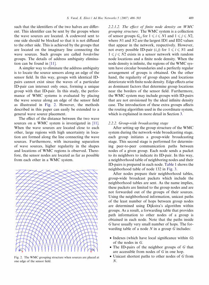
A simpler way to eliminate the address ambiguityis to locate the source sensors along an edge of thesensor field. In this way, groups with identical ID-pairs cannot exist since the waves of a particularID-pair can intersect only once, forming a uniquegroup with that ID-pair. In this study, the perfor-mance of WMC systems is evaluated by placingthe wave source along an edge of the sensor fieldas illustrated in Fig. 2. However, the methodsdescribed in this paper can easily be extended to ageneral wave source placement.

The effect of the distance between the two wavesources on a WMC system is investigated in [11].When the wave sources are located close to eachother, large regions with high uncertainty in loca-tion are formed along the line connecting the wavesources. Furthermore, with increasing separationof wave sources, higher regularity in the shapesand locations of WMC regions is observed. There-fore, the sensor nodes are located as far as possiblefrom each other in a WMC system.

WS1 WS2

Fig. 2. The WMC grouping structure when sources are placed atone edge of the sensor field.

2.2.1.2. The effect of finite node density on WMC

grouping structure. The WMC system is a collectionof sensor groups Gi,j for 1 6 i 6 N1 and 1 6 j 6 N2,where N1 and N2 are the largest ID1 and ID2 valuesthat appear in the network, respectively. However,not every possible ID-pair (i, j) for 1 6 i 6 N1 and1 6 j 6 N2 exists in a sensor network with randomnode locations and a finite node density. When thenode density is infinite, the regions of the WMC sys-tem have circular boundaries and a perfectly regulararrangement of groups is obtained. On the otherhand, the regularity of group shapes and locationsdeteriorate with finite node density. Edge effects ariseas dominant factors that determine group locationsnear the borders of the sensor field. Furthermore,the WMC system may include groups with ID-pairsthat are not envisioned by the ideal infinite densitycase. The introduction of these extra groups affectsthe routing algorithm used in the coordinate system,which is explained in more detail in Section 3.

2.2.2. Group-wide broadcasting stage

After setting up the group structure of the WMCsystem during the network-wide broadcasting stage,each group initiates a group-wide broadcastingstage. This second stage is performed for determin-ing peer-to-peer communication paths betweennodes of a given group. Each node sends a packetto its neighbors to indicate its ID-pair. In this way,a neighborhood table of neighboring nodes and theirID-pairs is prepared in each node. Table 1 shows theneighborhood table of node 132 in Fig. 3.

After nodes prepare their neighborhood tables,group-wide broadcast packets which include theneighborhood tables are sent. As the name implies,these packets are limited to the group nodes and arenot forwarded out of the groups of their sources.Using the neighborhood information, unicast pathsof the least number of hops between group nodesare determined using Dijkstra’s algorithm withingroups. As a result, a forwarding table that providespath information to other nodes of a group isobtained in each node. Note that the paths insideG have usually very small number of hops. The for-warding table of a node N in a group G includes:

• Indexes (which have local significance within G)of the nodes in G.

• The ID-pairs of the neighbor groups of G thatare accessible from nodes of G in one hop.

• Unicast shortest paths to other nodes of G fromN.

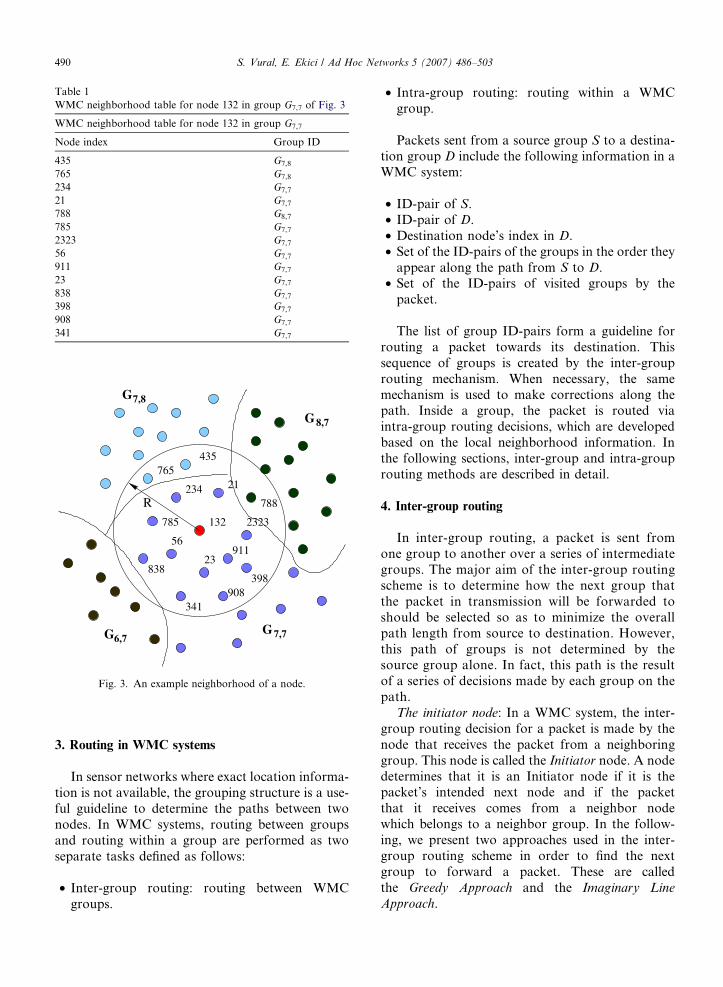
Table 1WMC neighborhood table for node 132 in group G7,7 of Fig. 3

WMC neighborhood table for node 132 in group G7,7

Node index Group ID

435 G7,8

765 G7,8

234 G7,7

21 G7,7

788 G8,7

785 G7,7

2323 G7,7

56 G7,7

911 G7,7

23 G7,7

838 G7,7

398 G7,7

908 G7,7

341 G7,7

234

785

83823

2323

21765

435

908398

341

56

132

788

911

G

G

GG

7,8

8,7

7,76,7

R

Fig. 3. An example neighborhood of a node.


3. Routing in WMC systems

In sensor networks where exact location informa-tion is not available, the grouping structure is a use-ful guideline to determine the paths between twonodes. In WMC systems, routing between groupsand routing within a group are performed as twoseparate tasks defined as follows:

• Inter-group routing: routing between WMCgroups.

• Intra-group routing: routing within a WMCgroup.

Packets sent from a source group S to a destina-tion group D include the following information in aWMC system:

• ID-pair of S.• ID-pair of D.• Destination node’s index in D.• Set of the ID-pairs of the groups in the order they

appear along the path from S to D.• Set of the ID-pairs of visited groups by the

packet.

The list of group ID-pairs form a guideline forrouting a packet towards its destination. Thissequence of groups is created by the inter-grouprouting mechanism. When necessary, the samemechanism is used to make corrections along thepath. Inside a group, the packet is routed viaintra-group routing decisions, which are developedbased on the local neighborhood information. Inthe following sections, inter-group and intra-grouprouting methods are described in detail.

4. Inter-group routing

In inter-group routing, a packet is sent fromone group to another over a series of intermediategroups. The major aim of the inter-group routingscheme is to determine how the next group thatthe packet in transmission will be forwarded toshould be selected so as to minimize the overallpath length from source to destination. However,this path of groups is not determined by thesource group alone. In fact, this path is the resultof a series of decisions made by each group on thepath.

The initiator node: In a WMC system, the inter-group routing decision for a packet is made by thenode that receives the packet from a neighboringgroup. This node is called the Initiator node. A nodedetermines that it is an Initiator node if it is thepacket’s intended next node and if the packetthat it receives comes from a neighbor nodewhich belongs to a neighbor group. In the follow-ing, we present two approaches used in the inter-group routing scheme in order to find the nextgroup to forward a packet. These are calledthe Greedy Approach and the Imaginary Line

Approach.

WS1WS2

G7,7

G13,9

G8,8

G8,7G7,8

G9,9 G10,8

G10,9

G11,9

G12,9

G12,10G11,10

G10,7G9,7

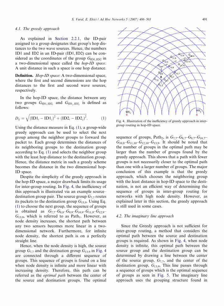
Fig. 4. Illustration of the inefficiency of greedy approach in inter-group routing in hop-ID space.


4.1. The greedy approach

As explained in Section 2.2.1, the ID-pairassigned to a group designates that group’s hop dis-tances to the two wave sources. Hence, the numbersID1 and ID2 in an ID-pair (ID1, ID2) can be con-sidered as the coordinates of the group GID1,ID2 ina two-dimensional space called the hop-ID space.A unit distance in such a space is one hop distance.

Definition. Hop-ID space: A two-dimensional space,where the first and second dimensions are the hopdistances to the first and second wave sources,respectively.

In the hop-ID space, the distance between anytwo groups GID1i;ID2i and GID1j;ID2j is defined asfollows:

Dij ¼ffiffiffiffiffiffiffiffiffiffiffiffiffiffiffiffiffiffiffiffiffiffiffiffiffiffiffiffiffiffiffiffiffiffiffiffiffiffiffiffiffiffiffiffiffiffiffiffiffiffiffiffiffiffiffiffiffiffiffiffiffiffiffiffiffiffiffiðID1i � ID1jÞ2 þ ðID2i � ID2jÞ2

q. ð1Þ

Using the distance measure in Eq. (1), a group-widegreedy approach can be used to select the nextgroup among the neighbor groups to forward thepacket to. Each group determines the distances ofits neighboring groups to the destination groupaccording to Eq. (1) and selects the neighbor groupwith the least hop distance to the destination group.Hence, the distance metric in such a greedy schemebecomes the distance in the two dimensional hop-ID space.

Despite the simplicity of the greedy approach inthe hop-ID space, a major drawback limits its usagefor inter-group routing. In Fig. 4, the inefficiency ofthis approach is illustrated via an example source–destination group pair. The source group G7,7 routesits packets to the destination group G13,9. Using Eq.(1) to choose the next group, the sequence of groupsis obtained as G7,7–G8,8–G9,9–G10,9–G11,9–G12,9–G13,9, which is referred to as Path1. However, asnode density increases, the shortest path betweenany two sensors becomes more linear in a two-dimensional network. Furthermore, for infinitenode density, the shortest path is on a perfectlystraight line.

Hence, when the node density is high, the sourcegroup G7,7 and the destination group G13,9 in Fig. 4are connected through a different sequence ofgroups. This sequence of groups is found on a linewhen node density is infinite and more linear withincreasing density. Therefore, this path can bereferred as the optimal path between the center ofthe source and destination groups. The optimal

sequence of groups, Path2, is G7,7–G8,7–G9,7–G10,7–G10,8–G11,10–G12,10–G13,9. It should be noted thatthe number of groups in the optimal path may belarger than the number of groups found by thegreedy approach. This shows that a path with fewergroups is not necessarily closer to the optimal paththan one with a larger number of groups. The majorconclusion of this example is that the greedyapproach, which chooses the neighboring groupwith the least distance in hop-ID space to the desti-nation, is not an efficient way of determining thesequence of groups in inter-group routing fornetworks with high node density. However, asexplained later in this section, the greedy approachis still used in some cases.

4.2. The imaginary line approach

Since the Greedy approach is not sufficient forinter-group routing, a method that considers theoptimal path between the source and destinationgroups is required. As shown in Fig. 4, when nodedensity is infinite, this optimal path between thesource group and the destination group can bedetermined by drawing a line between the centerof the source group, G7,7, and the center of thedestination group, G13,9. This line passes througha sequence of groups which is the optimal sequenceof groups as seen in Fig. 5. The imaginary lineapproach uses the grouping structure found in

G13,11

G6,8

WS1WS2

G12,10G11,10

G10,9G9,9

G8,8

G7,8

G12,11

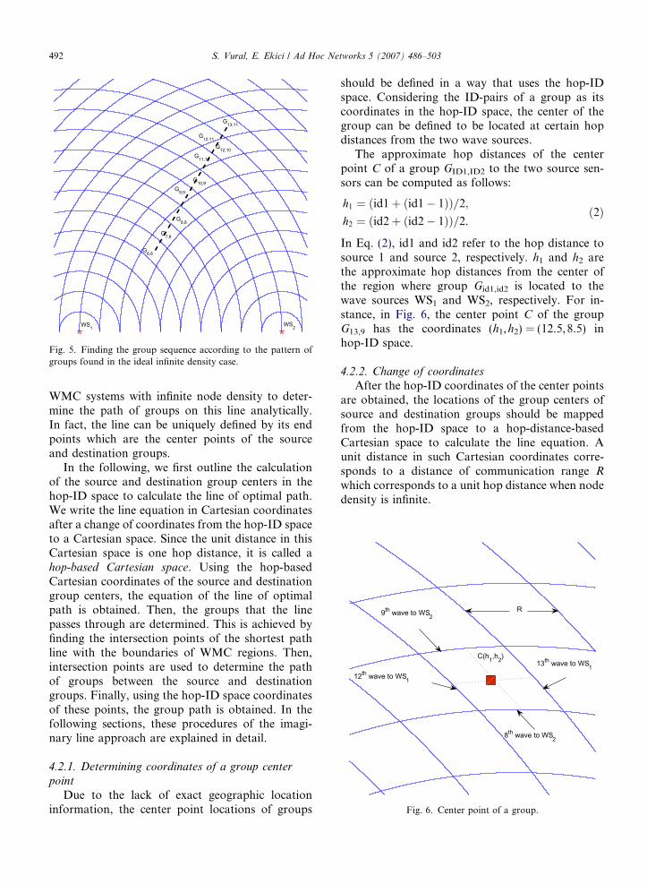
Fig. 5. Finding the group sequence according to the pattern ofgroups found in the ideal infinite density case.

13th wave to WS112th wave to WS1

9th wave to WS2

8th wave to WS2

C(h1,h2)

R

Fig. 6. Center point of a group.


WMC systems with infinite node density to deter-mine the path of groups on this line analytically.In fact, the line can be uniquely defined by its endpoints which are the center points of the sourceand destination groups.

In the following, we first outline the calculationof the source and destination group centers in thehop-ID space to calculate the line of optimal path.We write the line equation in Cartesian coordinatesafter a change of coordinates from the hop-ID spaceto a Cartesian space. Since the unit distance in thisCartesian space is one hop distance, it is called ahop-based Cartesian space. Using the hop-basedCartesian coordinates of the source and destinationgroup centers, the equation of the line of optimalpath is obtained. Then, the groups that the linepasses through are determined. This is achieved byfinding the intersection points of the shortest pathline with the boundaries of WMC regions. Then,intersection points are used to determine the pathof groups between the source and destinationgroups. Finally, using the hop-ID space coordinatesof these points, the group path is obtained. In thefollowing sections, these procedures of the imagi-nary line approach are explained in detail.

4.2.1. Determining coordinates of a group center

point

Due to the lack of exact geographic locationinformation, the center point locations of groups

should be defined in a way that uses the hop-IDspace. Considering the ID-pairs of a group as itscoordinates in the hop-ID space, the center of thegroup can be defined to be located at certain hopdistances from the two wave sources.

The approximate hop distances of the centerpoint C of a group GID1,ID2 to the two source sen-sors can be computed as follows:

h1 ¼ ðid1þ ðid1� 1ÞÞ=2;

h2 ¼ ðid2þ ðid2� 1ÞÞ=2.ð2Þ

In Eq. (2), id1 and id2 refer to the hop distance tosource 1 and source 2, respectively. h1 and h2 arethe approximate hop distances from the center ofthe region where group Gid1,id2 is located to thewave sources WS1 and WS2, respectively. For in-stance, in Fig. 6, the center point C of the groupG13,9 has the coordinates (h1,h2) = (12.5,8.5) inhop-ID space.

4.2.2. Change of coordinates

After the hop-ID coordinates of the center pointsare obtained, the locations of the group centers ofsource and destination groups should be mappedfrom the hop-ID space to a hop-distance-basedCartesian space to calculate the line equation. Aunit distance in such Cartesian coordinates corre-sponds to a distance of communication range R

which corresponds to a unit hop distance when nodedensity is infinite.

WS1(x1,y1) WS2(x2,y2)

C(x,y)

Inter—Source Hop Distancex

y

h2 hopsh1 hops

id2id1

Fig. 7. The illustration of the variables for finding the approx-imate coordinates of the center point of a sample group.


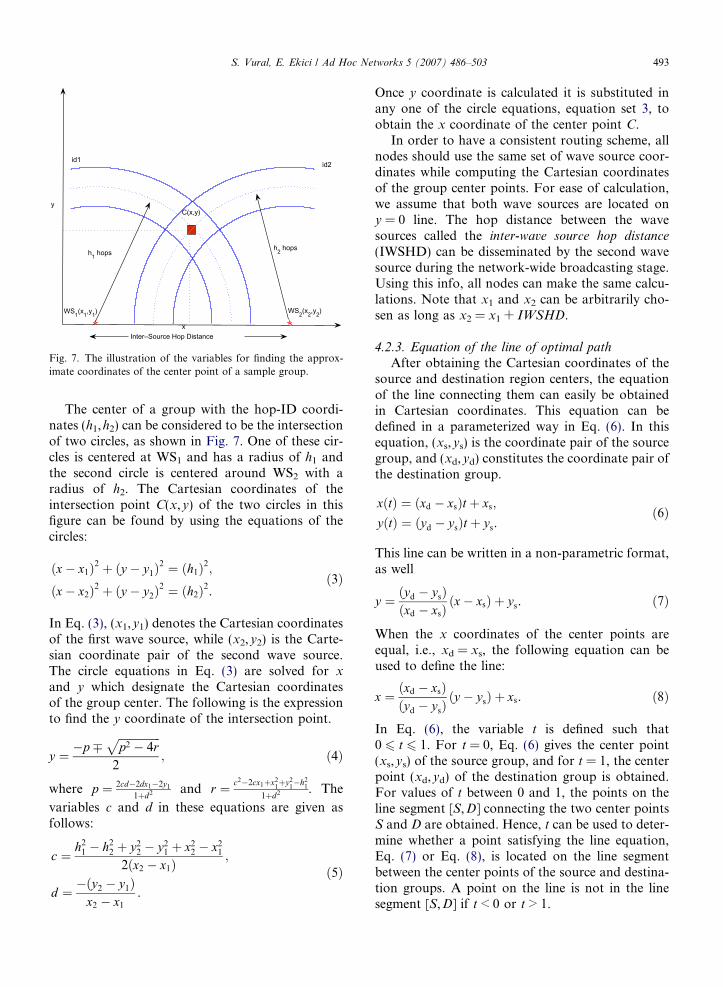
The center of a group with the hop-ID coordi-nates (h1,h2) can be considered to be the intersectionof two circles, as shown in Fig. 7. One of these cir-cles is centered at WS1 and has a radius of h1 andthe second circle is centered around WS2 with aradius of h2. The Cartesian coordinates of theintersection point C(x,y) of the two circles in thisfigure can be found by using the equations of thecircles:

ðx� x1Þ2 þ ðy � y1Þ2 ¼ ðh1Þ2;

ðx� x2Þ2 þ ðy � y2Þ2 ¼ ðh2Þ2.

ð3Þ

In Eq. (3), (x1,y1) denotes the Cartesian coordinatesof the first wave source, while (x2,y2) is the Carte-sian coordinate pair of the second wave source.The circle equations in Eq. (3) are solved for x

and y which designate the Cartesian coordinatesof the group center. The following is the expressionto find the y coordinate of the intersection point.

y ¼ �p �ffiffiffiffiffiffiffiffiffiffiffiffiffiffiffip2 � 4r

p2

; ð4Þ

where p ¼ 2cd�2dx1�2y1

1þd2 and r ¼ c2�2cx1þx21þy2

1�h2

1

1þd2 . The

variables c and d in these equations are given asfollows:

c ¼ h21 � h2

2 þ y22 � y2

1 þ x22 � x2

1

2ðx2 � x1Þ;

d ¼ �ðy2 � y1Þx2 � x1

.

ð5Þ

Once y coordinate is calculated it is substituted inany one of the circle equations, equation set 3, toobtain the x coordinate of the center point C.

In order to have a consistent routing scheme, allnodes should use the same set of wave source coor-dinates while computing the Cartesian coordinatesof the group center points. For ease of calculation,we assume that both wave sources are located ony = 0 line. The hop distance between the wavesources called the inter-wave source hop distance

(IWSHD) can be disseminated by the second wavesource during the network-wide broadcasting stage.Using this info, all nodes can make the same calcu-lations. Note that x1 and x2 can be arbitrarily cho-sen as long as x2 = x1 + IWSHD.

4.2.3. Equation of the line of optimal path

After obtaining the Cartesian coordinates of thesource and destination region centers, the equationof the line connecting them can easily be obtainedin Cartesian coordinates. This equation can bedefined in a parameterized way in Eq. (6). In thisequation, (xs,ys) is the coordinate pair of the sourcegroup, and (xd,yd) constitutes the coordinate pair ofthe destination group.

xðtÞ ¼ ðxd � xsÞt þ xs;

yðtÞ ¼ ðyd � ysÞt þ ys.ð6Þ

This line can be written in a non-parametric format,as well

y ¼ ðyd � ysÞðxd � xsÞ

ðx� xsÞ þ ys. ð7Þ

When the x coordinates of the center points areequal, i.e., xd = xs, the following equation can beused to define the line:

x ¼ ðxd � xsÞðyd � ysÞ

ðy � ysÞ þ xs. ð8Þ

In Eq. (6), the variable t is defined such that0 6 t 6 1. For t = 0, Eq. (6) gives the center point(xs,ys) of the source group, and for t = 1, the centerpoint (xd,yd) of the destination group is obtained.For values of t between 0 and 1, the points on theline segment [S,D] connecting the two center pointsS and D are obtained. Hence, t can be used to deter-mine whether a point satisfying the line equation,Eq. (7) or Eq. (8), is located on the line segmentbetween the center points of the source and destina-tion groups. A point on the line is not in the linesegment [S,D] if t < 0 or t > 1.


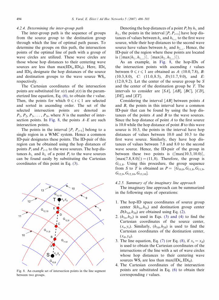
4.2.4. Determining the inter-group path

The inter-group path is the sequence of groupsfrom the source group to the destination groupthrough which the line of optimal path passes. Todetermine the groups on this path, the intersectionpoints of the optimal line of path with a group ofwave circles are utilized. These wave circles arethose whose hop distances to their centering wavesources are less than max(IDis, IDid). Here, IDisand IDid designate the hop distances of the sourceand destination groups to the wave source WSi,respectively.

The Cartesian coordinates of the intersectionpoints are substituted for x(t) and y(t) in the param-eterized line equation, Eq. (6), to obtain the t value.Then, the points for which 0 6 t 6 1 are selectedand sorted in ascending order. The set of theselected intersection points are denoted asP1, P2, P3, . . . , PN, where N is the number of inter-section points. In Fig. 8, the points A–E are suchintersection points.

The points in the interval [Pi Pi+1] belong to asingle region in a WMC system. Hence a commonID-pair designates these points. The ID-pair of thisregion can be obtained using the hop distances ofpoints Pi and Pi+1 to the wave sources. The hop dis-tances h1i and h2i of a point Pi to the wave sourcescan be found easily by substituting the Cartesiancoordinates of this point in Eq. (3).

G13,10

G10,8

13

9

8

10

10

11

12

A

C

B

D

E

xd,yd

xs,ys

G11,8

G12,10

G12,9

G11,9

T

S

Fig. 8. An example set of intersection points in the line segmentbetween two groups.

Denoting the hop distances of a point Pi by h1i andh2i , the points in the interval [Pi Pi+1] have hop dis-tances of values between h1i and h1iþ1

to the first wavesource, while their hop distances to the second wavesource have values between h2i and h2iþ1

. Hence, theID-pair of the region where these points are locatedis ðdmaxðh1i ; h1iþ1

Þe; dmaxðh2i ; h2iþ1ÞeÞ.

As an example, in Fig. 8, the hop-IDs ofthe intersection points with ascending t valuesbetween 0 6 t 6 1 are obtained as A: (10.0,7.8), B:(10.3,8.0), C: (11.0,8.5), D:(11.7, 9.0), and E:(12.0,9.2). Let the center of the source group be Sand the center of the destination group be T. Theintervals to consider are [SA], [AB], [BC], [CD],[DE], and [ET].

Considering the interval [AB] between points A

and B, the points in this interval have a commonID-pair that can be found by using the hop dis-tances of the points A and B to the wave sources.Since the hop distance of point A to the first sourceis 10.0 while the hop distance of point B to this wavesource is 10.3, the points in the interval have hopdistances of values between 10.0 and 10.3 to thefirst wave source. Similarly, they have hop dis-tances of values between 7.8 and 8.0 to the secondwave source. Hence, the ID-pair of the group inbetween these two points is (dmax(10.3,10.0)e,dmax(7.8, 8.0)e) = (11, 8). Therefore, the group isG11,8. Using this procedure, the group sequencefrom S to T is obtained as P = [G10,8,G11,8,G11,9,G12,9,G12,10,G13,10].

4.2.5. Summary of the imaginary line approach

The imaginary line approach can be summarizedin the following steps of operations:

1. The hop-ID space coordinates of source groupcenter S(h1s,h2s) and destination group centerD(h1d,h2d) are obtained using Eq. (2).

2. (h1s,h2s) is used in Eqs. (3) and (4) to find theCartesian coordinates of the source center,(xs,ys). Similarly, (h1d,h2d) is used to find theCartesian coordinates of the destination center,(xd,yd).

3. The line equation, Eq. (7) (or Eq. (8), if xs = xd)is used to obtain the Cartesian coordinates of theintersections of the line with a set of wave circleswhose hop distances to their centering wavesources WSi are less than max(IDis, IDid).

4. The Cartesian coordinates of the intersectionpoints are substituted in Eq. (6) to obtain theircorresponding t values.

WS

h 1

h2

IWSHD1 WS2

C(h1, h2)

Fig. 9. Triangularity condition for the group Gh1 ;h2.


5. All intersection points with 0 6 t 6 1 areretrieved to form a set of intersection pointsfound on the line segment connecting S and D.These points along with S and D are sorted inincreasing order of t values. Hence, the set{S,P1,P2, . . . , PN,D} is obtained, where ti < ti+1,ts = 0 and td = 1, for 1 6 i 6 N � 1.

6. The hop-ID space coordinates of Pi, for1 6 i 6 N, are obtained by substituting their cor-responding Cartesian coordinates in Eq. (3).

7. The hop-ID space coordinates of consecutivepairs of points in the set {S,P1,P2, . . . , PN,D}are used to determine the ID-pair of the groupsthrough which the line segment passes.

4.3. Combining the greedy and imaginary line

approaches: inter-group routing

The grouping structure of the WMC system isdesigned for the case when node density is assumedto be infinite. Hence, the imaginary line approachoutlined in Section 4.2 is derived using an ideal

group pattern. However, when the node density isfinite, group locations and shapes are not as regularas they are in the ideal infinite density case.Furthermore, some of the groups that are envi-sioned in Fig. 5 may not exist in the WMC system.For instance, if group G3,4 has a neighbor groupG4,5 in the ideal infinite density case, there is noguarantee that these two groups are neighboringgroups in case of finite node density. Moreover,either or both of the groups may not exist at all.Due to these reasons, the routing scheme of theWMC systems should be able to handle the irregu-larities that emerge as a result of finite nodedensity.

4.3.1. Two types of WMC groups

When node density is finite, some extra groupsmay emerge other than the ones that are found inthe infinite node density case. Since the inter-grouprouting scheme makes use of the regularity of thegroup pattern of WMC systems when node densityis infinite, there should be mechanisms to deal withthe irregularity induced by the existence of theseextra groups. As a first step, the system should differ-entiate between two types of groups, namely,regular groups and irregular groups.

The following are the definitions of these two dif-ferent group types that can be found in a finite den-sity WMC system:

• Regular group: A group that exists in the WMCsystem in case of infinite node density.

• Irregular group: A group that cannot normallyexist in the WMC system in case of infinite nodedensity.

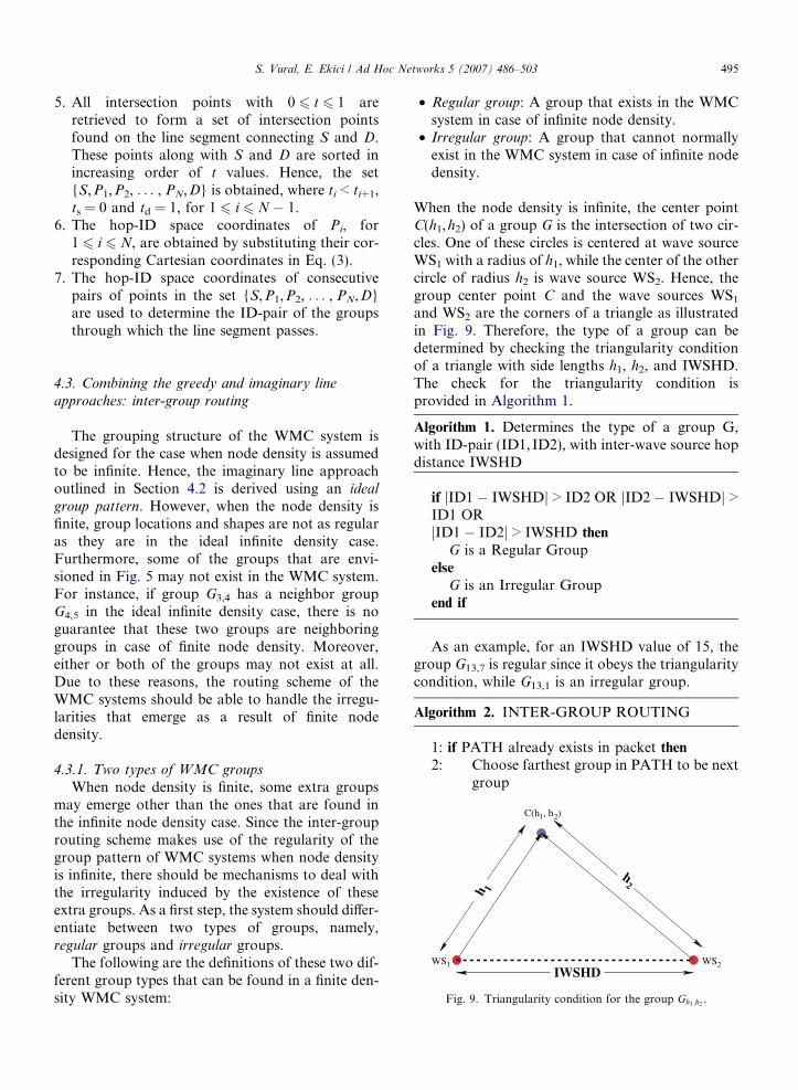
When the node density is infinite, the center pointC(h1,h2) of a group G is the intersection of two cir-cles. One of these circles is centered at wave sourceWS1 with a radius of h1, while the center of the othercircle of radius h2 is wave source WS2. Hence, thegroup center point C and the wave sources WS1

and WS2 are the corners of a triangle as illustratedin Fig. 9. Therefore, the type of a group can bedetermined by checking the triangularity conditionof a triangle with side lengths h1, h2, and IWSHD.The check for the triangularity condition isprovided in Algorithm 1.

Algorithm 1. Determines the type of a group G,with ID-pair (ID1, ID2), with inter-wave source hopdistance IWSHD

if jID1 � IWSHDj > ID2 OR jID2 � IWSHDj >ID1 ORjID1 � ID2j > IWSHD then

G is a Regular Groupelse

G is an Irregular Groupend if

As an example, for an IWSHD value of 15, thegroup G13,7 is regular since it obeys the triangularitycondition, while G13,1 is an irregular group.

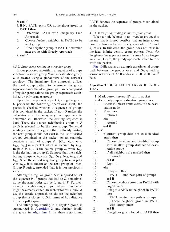
Algorithm 2. INTER-GROUP ROUTING

1: if PATH already exists in packet then

2: Choose farthest group in PATH to be nextgroup


3: end if

4: if No PATH exists OR no neighbor group inPATH then

5: Determine PATH with Imaginary LineApproach

6: Choose farthest neighbor in PATH to benext group

7: If no neighbor group in PATH, determinenext group with Greedy Approach

8: end if

4.3.2. Inter-group routing in a regular group

In our proposed algorithm, a sequence of groupsP between a source group S and a destination groupD is created using a global view of the networktopology. The imaginary line approach utilizesthe ideal group pattern to determine this groupsequence. Since the ideal group pattern is composedof regular groups alone, the group sequence is estab-lished by only regular groups.

Upon the reception of a packet, a regular groupG performs the following operations: First, thepacket is checked whether a sequence of groupsP is contained in the packet. If not, G makes thecalculations of the imaginary line approach todetermine P. Otherwise, the existing sequence iskept. Then, the nearest neighboring group in P

to D is selected to be the next group. To avoidsending a packet to a group that is already visited,the next group should not exist in the list of visitedgroups contained in the packet. As an example,consider a path of groups P= [G3,4, G4,5, G5,5,G5,4, G5,6] in a packet which is received by G4,5.In path P, G3,4 is the source group S, while G5,6

is the destination group D. Suppose that the neigh-boring groups of G4,5 are G4,4, G3,5, G5,5, G5,4, andG5,3. Since the closest neighbor group to D in pathP is G5,4, it is chosen as the next group of Inter-Group Routing, provided that it is not previouslyvisited.

Although a regular group G is supposed to setthe sequence P of groups that lead to D, sometimesno neighboring nodes can be found in P. Further-more, all neighboring groups that are found in P

might be already visited. In such instances, G shoulduse the greedy approach to choose the neighborgroup that is closest to D in terms of hop distancein the hop-ID space.

The inter-group routing in a regular group issummarized in Algorithm 2, and further detailsare given in Algorithm 3. In these algorithms,

PATH denotes the sequence of groups P containedin the packet.

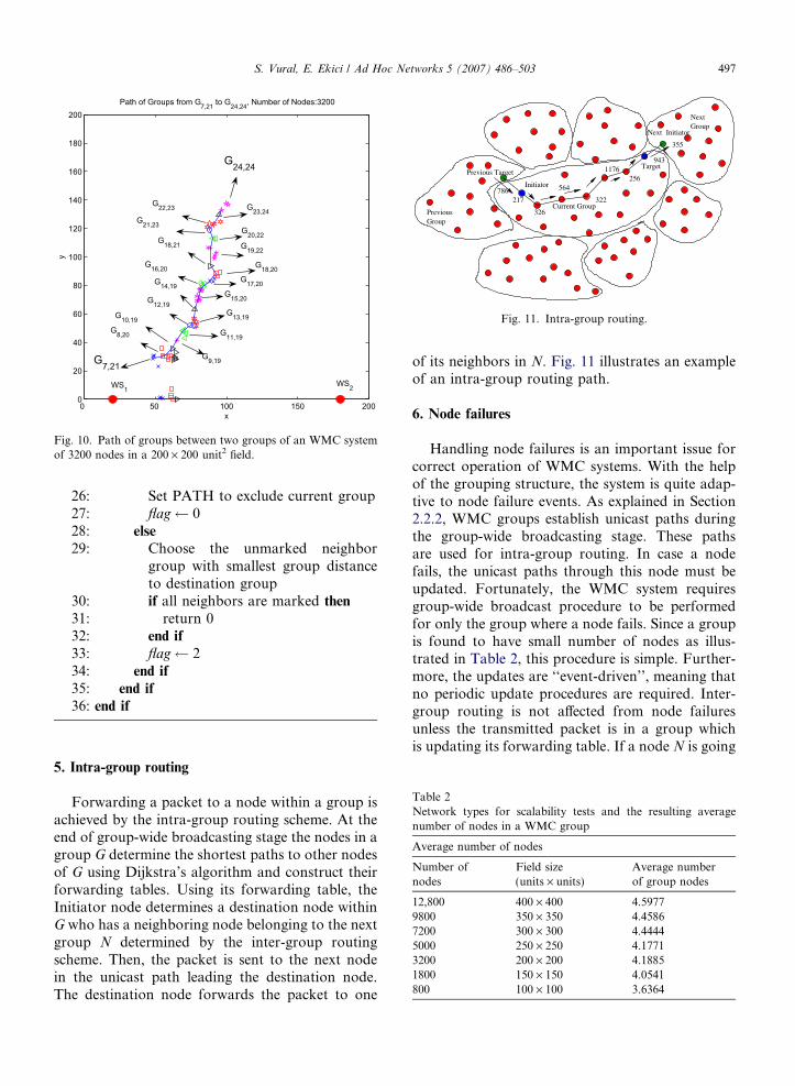
4.3.3. Inter-group routing in an irregular groupWhen a node belongs to an irregular group, this

means that it is not possible that an intersectionpoint of two circles with the given radii of h1 andh2 exists. In this case, the group does not exist inthe ideal infinite density group pattern. Thus, the

imaginary line approach cannot be used by an irregu-

lar group. Hence, the greedy approach is used to for-ward the packet.

Fig. 10 illustrates an example experimental grouppath between the groups G7,21 and G24,24 with asensor network of 3200 nodes in a 200 · 200 unit2

field.

Algorithm 3. DETAILED INTER-GROUP ROU-TING

1: Mark current group ID-pair in packet2: if currentgroup = destination group then

3: Check if unicast route exists to the desti-nation node

4: if yes then5: return 16: else

7: return 08: end if

9: else

10: if current group does not exist in idealgraph then

11: Choose the unmarked neighbor groupwith smallest group distance to desti-nation group

12: if all neighbors are marked then


15: flag 116: else

17: if flag = 1 then18: PATH find new path of groups19: end if

20: Choose neighbor group in PATH withlargest index

21: if flag = 2 AND no neighbor in PATHthen

22: PATH find new path of groups23: Choose neighbor group in PATH

with largest index24: end if

25: if neighbor group found in PATH then

Initiator

Target

Group

PreviousGroup

Next

Target

Next

Previous

Current Group

Initiator

326

564

322

1176256

943

217

355

786

Fig. 11. Intra-group routing.

0 50 100 150 2000

20

40

60

80

100

120

140

160

180

200Path of Groups from G7,21 to G24,24, Number of Nodes:3200

x

y

G7,21

G8,20

G15,20

G16,20

G13,19

G14,19

G11,19

G9,19

G12,19

G10,19

G24,24

G23,24G22,23

G21,23G20,22

G19,22G18,21

G18,20G17,20

WS1WS2

Fig. 10. Path of groups between two groups of an WMC systemof 3200 nodes in a 200 · 200 unit2 field.


26: Set PATH to exclude current group27: flag 028: else

29: Choose the unmarked neighborgroup with smallest group distanceto destination group

30: if all neighbors are marked then


33: flag 234: end if

35: end if

36: end if

Table 2Network types for scalability tests and the resulting averagenumber of nodes in a WMC group

Average number of nodes

Number ofnodes

Field size(units · units)

Average numberof group nodes

12,800 400 · 400 4.59779800 350 · 350 4.45867200 300 · 300 4.44445000 250 · 250 4.17713200 200 · 200 4.18851800 150 · 150 4.0541800 100 · 100 3.6364

5. Intra-group routing

Forwarding a packet to a node within a group isachieved by the intra-group routing scheme. At theend of group-wide broadcasting stage the nodes in agroup G determine the shortest paths to other nodesof G using Dijkstra’s algorithm and construct theirforwarding tables. Using its forwarding table, theInitiator node determines a destination node withinG who has a neighboring node belonging to the nextgroup N determined by the inter-group routingscheme. Then, the packet is sent to the next nodein the unicast path leading the destination node.The destination node forwards the packet to one

of its neighbors in N. Fig. 11 illustrates an exampleof an intra-group routing path.

6. Node failures

Handling node failures is an important issue forcorrect operation of WMC systems. With the helpof the grouping structure, the system is quite adap-tive to node failure events. As explained in Section2.2.2, WMC groups establish unicast paths duringthe group-wide broadcasting stage. These pathsare used for intra-group routing. In case a nodefails, the unicast paths through this node must beupdated. Fortunately, the WMC system requiresgroup-wide broadcast procedure to be performedfor only the group where a node fails. Since a groupis found to have small number of nodes as illus-trated in Table 2, this procedure is simple. Further-more, the updates are ‘‘event-driven’’, meaning thatno periodic update procedures are required. Inter-group routing is not affected from node failuresunless the transmitted packet is in a group whichis updating its forwarding table. If a node N is going


to send a packet to a group, say G, and G is updat-ing its forwarding table because of a node failure,then N stores the packet temporarily and sends itto G when the update procedure is over.

7. Comparative performance evaluation

In this section, the performance of the WMC sys-tem is evaluated in terms of the packet transmissionsuccess rate and the average path length. The per-formance results of WMC system are comparedwith those of greedy geographic routing (GGR)and the virtual coordinate scheme (GWL, geo-graphic routing without location information)introduced in [10]. The comparisons are based oncommunication overhead, complexity, and routingperformance. The effects of node density and thesize of the sensor network field (scalability) on rout-ing performance are investigated by changing thenumber nodes and/or the field size. Table 2 showsdifferent types of networks used in scalability tests.The change of node density is studied using the setof networks as shown in Table 3.

The sensor nodes in the simulations have identi-cal circular communication ranges with radiusR = 8 units and symmetric communication links.The effects of fading, interference, and asymmetriclinks are not included in this study and can be inves-tigated as a future research. Nodes can transmit/receive packets without error to/from within acommunication range of radius R. Furthermore,sensor locations are random with a two dimensionalPoisson distribution.

7.1. The geographic routing without location

information scheme (GWL)

The GWL scheme [10] makes use of the neigh-borhood information of sensors to create a virtual

Table 3Network types for tests of the effect of node density

Network types for density tests

Number of nodes Network size (unit2)

3200 125 · 1253200 150 · 1503200 175 · 1753200 200 · 2003200 225 · 2253200 250 · 250

coordinate space. In this way, although the sensorslack location information, greedy geographic rout-ing can be performed over these new virtual coordi-nates. These coordinates are determined using thenodes in the perimeter of the network, called theperimeter nodes.

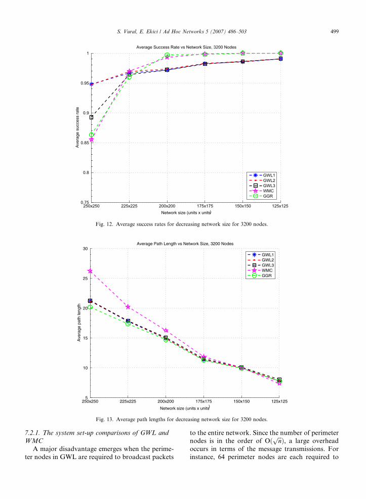
GWL proposes three schemes based on the infor-mation available in the nodes. In the first schemeperimeter nodes know that they are perimeter nodesand are aware of their true geographic coordinates.In the second scheme, perimeter nodes know thatthey are perimeter nodes but they do not know theirlocations. Finally, in the third scheme, perimeternodes neither know their coordinates nor the factthat they are perimeter nodes. The results of thesethree different GWL schemes are labeled asGWL1, GWL2, and GWL3 in Figs. 12–15.

The procedure of GWL3, which is the GWLmethod with the least available location informa-tion, can be outlined as follows [10]:

1. Two designated bootstrap beacon nodes broad-cast to the entire network. Nodes use their dis-tances to one of these bootstrap nodes todetermine whether they are perimeter nodes.

2. Every perimeter node sends a broadcast messageto the entire network to enable every other nodeto compute its perimeter vector, i.e., the distancesfrom that node to all perimeter nodes.

3. Perimeter and bootstrap nodes broadcast theirperimeter vectors to the entire network.

4. Each node uses these inter-perimeter distances tocompute the coordinates for both itself and theperimeter nodes.

5. Locations of the perimeter nodes are not changedwhile all non-perimeter nodes run a relaxationalgorithm to determine their virtual coordinates.At each step of this algorithm, a non-perimeternode calculates the average of the x coordinatesof its neighboring nodes and assigns this valueto its x coordinate. The same averaging is per-formed for the y coordinate.

7.2. The comparison of the system set-up

complexities of GWL and WMC

The GWL scheme is found to have lower successrates and comparable average path lengths when theresults of GGR are considered. However, the GWLscheme has also the following drawbacks during itssystem set-up phase.

250x250 225x225 200x200 175x175 150x150 125x1250.75

0.8

0.85

0.9

0.95

1

Network size (units x units)

Aver

age

succ

ess

rate

Average Success Rate vs Network Size, 3200 Nodes

GWL1GWL2GWL3WMCGGR

Fig. 12. Average success rates for decreasing network size for 3200 nodes.

250x250 225x225 200x200 175x175 150x150 125x1255

10

15

20

25

30

Network size (units x units)

Ave

rage

pat

h le

ngth

Average Path Length vs Network Size, 3200 Nodes

GWL1GWL2GWL3WMCGGR

Fig. 13. Average path lengths for decreasing network size for 3200 nodes.


7.2.1. The system set-up comparisons of GWL and

WMC

A major disadvantage emerges when the perime-ter nodes in GWL are required to broadcast packets

to the entire network. Since the number of perimeternodes is in the order of Oð ffiffiffinp Þ, a large overheadoccurs in terms of the message transmissions. Forinstance, 64 perimeter nodes are each required to

800 1800 3200 5000 7200 9800 128000.85

0.9

0.95

1

Number of nodes

Aver

age

rate

Average Success Rate vs. Number of Nodes, Node Density = 0.08 nodes / m2

GWL1GWL2GWL3WMCGGR

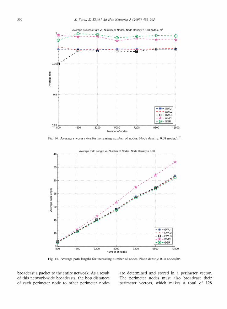
Fig. 14. Average success rates for increasing number of nodes. Node density: 0.08 nodes/m2.

800 1800 3200 5000 7200 9800 128005

10

15

20

25

30

35

40

Number of nodes

Aver

age

path

leng

th

Average Path Length vs. Number of Nodes, Node Density = 0.08

GWL1GWL2GWL3WMCGGR

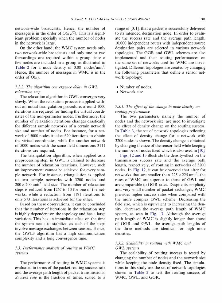
Fig. 15. Average path lengths for increasing number of nodes. Node density: 0.08 nodes/m2.


broadcast a packet to the entire network. As a resultof this network-wide broadcasts, the hop distancesof each perimeter node to other perimeter nodes

are determined and stored in a perimeter vector.The perimeter nodes must also broadcast theirperimeter vectors, which makes a total of 128


network-wide broadcasts. Hence, the number ofmessages is in the order of Oðn

ffiffiffinpÞ. This is a signif-

icant problem especially when the number of nodesin the network is large.

On the other hand, the WMC system needs onlytwo network-wide broadcasts and only one or twoforwardings are required within a group since afew nodes are included in a group as illustrated inTable 2 for a node density of 0.08 nodes/unit2.Hence, the number of messages in WMC is in theorder of O(n).

7.2.2. The algorithm convergence delay in GWL

relaxation step

The relaxation algorithm in GWL converges veryslowly. When the relaxation process is applied with-out an initial triangulation procedure, around 1000iterations are required for finding the virtual coordi-nates of the non-perimeter nodes. Furthermore, thenumber of relaxation iterations changes drasticallyfor different sample networks of a certain networksize and number of nodes. For instance, for a net-work of 5000 nodes it takes 620 iterations to obtainthe virtual coordinates, while for another networkof 5000 nodes with the same field dimensions 3111iterations are required.

The triangulation algorithm, when applied as apreprocessing step, in GWL is claimed to decreasethe number of relaxation iterations. However, suchan improvement cannot be achieved for every sam-ple network. For instance, triangulation is appliedto two sample networks with 3200 nodes and200 · 200 unit2 field size. The number of relaxationsteps is reduced from 1267 to 13 for one of the net-works, while a reduction from 1191 iterations toonly 573 iterations is achieved for the other.

Based on these observations, it can be concludedthat the number of iterations in the relaxation stepis highly dependent on the topology and has a largevariation. This has an immediate effect on the timethe system needs to stabilize, as each of the stepsinvolve message exchanges between sensors. Hence,the GWL3 algorithm has a high communicationcomplexity and a long convergence time.

7.3. Performance analysis of routing in WMC

systems

The performance of routing in WMC systems isevaluated in terms of the packet routing success rateand the average path length of packet transmissions.Success rate is the fraction of times, scaled to a

range of [0, 1], that a packet is successfully deliveredto its intended destination node. In order to evalu-ate the success rate and the average path length,10,000 independent routes with independent sourcedestination pairs are selected in various networktopologies. The GGR and GWL schemes are alsoimplemented and their routing performances onthe same set of networks used for WMC are inves-tigated. Different topologies are created by changingthe following parameters that define a sensor net-work topology:

• Number of nodes.• Network size.

7.3.1. The effect of the change in node density on

routing performance

The two parameters, namely the number ofnodes and the network size, are used to investigatethe effect of density change on the routing success.In Table 3, the set of network topologies reflectingthe effect of density change for a network with3200 nodes is shown. The density change is obtainedby changing the size of the sensor field while keepingthe number of nodes fixed which is also used in [10].

Figs. 12 and 13 illustrate the density-effect on thetransmission success rate and the average pathlength, respectively, of routing in networks of 3200nodes. In Fig. 12, it can be observed that after fornetworks that are smaller than 225 · 225 unit2, therates of WMC are superior to those of GWL andare comparable to GGR rates. Despite its simplicityand very small number of packet exchanges, WMCprovides higher success rates when compared withthe more complex GWL scheme. Decreasing thefield size, which is equivalent to increasing the den-sity, decreases the average path length of WMCsystem, as seen in Fig. 13. Although the averagepath length of WMC is slightly longer than thoseof GGR and GWL, the average path lengths ofthe three methods are identical for high nodedensities.

7.3.2. Scalability in routing with WMC and

GWL systems

The scalability of routing success is tested bychanging the number of nodes and the network sizewhile keeping the node density fixed. The simula-tions in this study use the set of network topologiesshown in Table 2 to test the routing success ofWMC, GWL, and GGR.


Results for the effect of network size (scalability)are similar to the results of the density effect onrouting when the WMC and the GWL systems arecompared. Despite the fact that increasing networksize causes an increase in average path length, therouting success rates of WMC are much better thanGWL and comparable to GGR. Figs. 14 and 15illustrate these findings of average success rate andpath length, respectively.

8. Conclusion

In this study, a simple and efficient coordinatesystem for dense sensor networks, the wavemapping coordinate system (WMC), is introduced.Furthermore, a highly successful and simple routingmechanism over WMC systems is designed. WMCsystem is aimed to provide approximate locationinformation and is a scalable coordinate systemfor sensor networks without location information,any infrastructure support or complex and expen-sive hardware availability. The performance of rout-ing over WMC systems is evaluated according tochanging node density and sensor field size. Theperformance results are compared with the geo-graphic routing without location information(GWL) scheme outlined in [10], and the geographicgreedy routing scheme (GGR) which uses real coor-dinate information of sensors.

The GWL scheme requires a large number ofpacket exchanges, along with the need for solvingcomplex optimization problems in each sensor node.The number of messages is in the order of Oðn ffiffiffi

np Þ in

the initial stage of virtual coordinate construction,which creates a broadcast storm in WSNs. On theother hand, the WMC system needs only two net-work-wide broadcasts with a complexity of O(n).Furthermore, group-wide broadcasts in WMCinvolve only the nodes of individual groups, whichleads to a very small number of packet forwardings.

Another problem encountered in GWL Systemsis the slow convergence of the relaxation algorithm,especially for networks with large number ofnodes. Hundreds or even thousands of relaxationiterations occur and each sensor nodes is requiredto send a packet to its neighbors in each relaxationiteration. Hence, GWL needs hundreds of packettransmissions for each node during the systemstart-up, which is a high overhead for a sensornetwork.

From the perspective of system simplicity, mes-sage complexity, and routing success rate, the

WMC system is found to be superior to the GWLscheme. The routing success rate of WMC is muchbetter than GWL and comparable to GGR. Despiteits simplicity and very small number of packetexchanges, WMC provides higher success rates whencompared with the more complex GWL scheme.

References

[1] P. Bose, P. Morin, I. Stojmenovic, J. Urrutia, Routing withguaranteed delivery in ad hoc wireless networks, WirelessNetworks 7 (2001) 609–616.

[2] J. Gao, L. Guibas, J. Hershburger, L. Zhang, A. Zhu,Geometric spanner for routing in mobile networks, in:Proceedings of the 2nd ACM Symposium on Mobile Ad HocNetworking and Computing (MobiHoc 2001), October,2001, pp. 45–55.

[3] W.-H. Liao, J.-P. Sheu, Y.-C. Tseng, Grid: a fully location-aware routing protocol for mobile ad hoc networks, Tele-communication Systems 18 (2001) 37–60.

[4] B. Karp, H. Kung, Greedy perimeter stateless routing forwireless networks, in: Proceedings of IEEE/ACM Mobicom2000, 2000, pp. 243–254.

[5] B. Hoffman-Wellendorf, H. Lichtennegger, J. Collins,Global Positioning System: Theory and Practice, fourthed., Springer Verlag, 1997.

[6] N. Bulusu, J. Heidemann, D. Estrin, Gps-less low-costoutdoor localization for very small devices, IEEE PersonalCommunications 7 (October) (2000) 28–34.

[7] S. Capkun, M. Hamdi, J. Hubbaux, Gps-free positioning inmobile ad hoc networks, in: The 34th IEEE HawaiiInternational Conference on System Sciences, 2001, pp.3481–3490.

[8] D. Niculescu, B. Nath, Localized positioning in ad hocnetworks, in: First IEEE International Workshop on SensorNetwork Protocols and Applications, October, 2003, pp. 42–50.

[9] D.S.J. De Couto, R. Morris, Location proxies and interme-diate node forwarding for practical geographic forwarding,mit-lcs-tr, MIT Laboratory for Computer Science, 2001.

[10] A. Rao, C. Papadimitriou, S. Ratnasamy, S. Shenker, I.Stoica, Geographic routing without location information, in:MobiCom, 2003.

[11] S. Vural, E. Ekici, Wave addressing for dense sensornetworks, in: Second International Workshop on Sensorand Actor Network Protocols and Applications (SANPA2004), August, 2004, pp. 56–66.

Serdar Vural is currently a Ph.D. studentat the Electrical and Computer Engi-neering Department, at The Ohio StateUniversity, Columbus, Ohio, USA. Hereceived his BS degree at the ElectricalEngineering Department, at the BogaziciUniversity, Istanbul, Turkey and his MSdegree at the Electrical and ComputerEngineering Department, at The OhioState University. His research interest isin sensor networks.


Eylem Ekici has received his BS and MSdegrees in Computer Engineering fromBogazici University, Istanbul, Turkey, in1997 and 1998, respectively. He receivedhis Ph.D. degree in Electrical and Com-puter Engineering from Georgia Insti-tute of Technology, Atlanta, GA, in2002. Currently, he is an AssistantProfessor in the Department of Electricaland Computer Engineering of The OhioState University, Columbus, OH. His

current research interests include wireless sensor networks, next

generation wireless systems, space-based networks, and vehicularcommunication systems, with a focus on routing and mediumaccess control protocols, resource management, and analysis ofnetwork architectures and protocols. He also conducts researchon interfacing of dissimilar networks.

Documents

Hop-distance based addressing and routing for dense sensor