Embed Size (px)
Citation preview

Hospital Staffing and Inpatient Mortality
Carlos Dobkin* University of California, Berkeley
This version: June 21, 2003
Abstract
Staff-to-patient ratios are a current policy concern in hospitals nationwide. Legislators in California and New York have imposed staffing requirements on hospitals that are estimated to cost hundreds of millions of dollars per year. These reforms were motivated by the presumption of a causal link between lower hospital staffing levels and adverse patient outcomes. However, the cited empirical evidence is based almost entirely on across-hospital comparisons, which is problematic if the nonrandom selection of patients into hospitals leads to unobservable differences across hospitals in patient characteristics and illness severity. By contrast, this paper uses the significant reduction in the number of doctors on staff on the weekend to estimate the effects of staffing on mortality rates. Within-hospital comparisons in outcome differences between weekday and weekend admissions have two advantages over previous research. First, the observable differences in patient characteristics are much smaller within hospitals than across hospitals. More importantly, it is possible to construct an index that corrects for biases due to unobservable selection into staffing regimes that is based on the excess share of admissions that occur on weekdays. Consistent with previous research, there is a robust association between excess mortality and weekend admission even after regression-adjustment. However, correcting for nonrandom selection in favor of weekday admissions leads to a finding of no excess mortality among patients admitted on the weekend. This suggests that despite a significant reduction in the number of doctors and services provided on the weekend, hospitals are effective in triaging patients with less severe conditions.
Keywords: Public Health, Hospital Staffing, Selection Correction JEL classification: I12, I18
* Dept. of Economics, University of California, Berkeley. Contact: [email protected]. 549
Evans Hall #3880, UC Berkeley, Berkeley, CA 94720-3880, USA. I would like to thank my thesis advisor Kenneth Chay and David Card, Jeffrey Gould M.D., Russell Green, David Lee, Nancy Nicossia, Emmanuel Saez, Paul Ware M.D. Jeffrey Weinstein

1. Introduction
Medical errors are currently a major concern to medical professionals and the public
at large. A 1999 Institute of Medicine Report, To Err is Human: Building a Safer Health System,
estimated that 44,000 to 98,000 hospital patients in the US are killed by medical errors each
year. The reaction to this study was rapid. Within two weeks Congress held hearings to
explore the feasibility of implementing the study’s suggestions.
The California legislature has also taken up this issue by passing legislation that
mandates minimum nurse-to-patient ratios. These rules, which go into effect in July 2003,
make California the first state to set hospital-wide minimum nurse-to-patient ratios. The
California Healthcare Association estimates that these changes will cost at least $400 million
to implement. A similar reform in New York State mandated changes in staffing rates and
work hours for doctors, with one goal being to increase both the number and seniority of
doctors on site at hospitals on the weekend. The estimated cost of implementing these
changes was $358 million per year in 1989 dollars (Thorpe 1990).
These reforms mandating increased staff-to-patient ratios have been motivated by
the presumption of a causal link between hospital staffing levels and adverse patient
outcomes. Although there have been several recent papers on this question, the existing
empirical evidence is somewhat limited. Most research has examined the across-hospital
association between staffing levels and inpatient mortality and morbidity – for example,
Aiken, et al. (JAMA 2002), Needelman, et al. (N England J Med 2002), and Pronovost, et al.
(JAMA 1999). However, these comparisons will lead to biased estimates if nonrandom
selection of patients into hospitals leads to unobservable differences across hospitals in
patient characteristics and illness severity. For example, patients with planned admissions
tend to be lower risk than patients admitted through the emergency room. Thus, hospitals
with established reputations and higher staffing levels will have a disproportionate share of
low risk admissions if patients with planned admissions sort to better-known hospitals. In
this case, the cross-sectional correlation between staffing levels and patient outcomes may be
spurious.
By contrast, Bell and Redelmeier (N England J Med, 2001) provide evidence on the
effects of reduced staffing within the same hospital over the weekly cycle. In particular, they
find that patients admitted to hospitals during the weekend have significantly higher
1

mortality rates than patients admitted on weekdays in Canada, even after adjustment for
observable patient characteristics. Since staffing levels within a hospital are lower during the
weekend, they conclude that the reduced staffing has negative effects. However, if patients
admitted on the weekend have more severe conditions than those admitted during the week,
then these estimates will be biased due to the unobservable sorting of patients across the
days of the week. This type of selection bias is plausible as the Canadian data show that a
disproportionate number of patients are admitted to hospitals on weekdays relative to the
weekend.
I use microdata on the universe of discharges from California hospitals between
1995 and 1999 to examine two questions: 1) “Is there a direct relationship between the
number of doctors on staff in a hospital and the probability that an error will occur that
results in a patient’s death?”; and 2) “Does a temporary reduction in the services hospitals
provide result in worse outcomes for patients admitted on the weekend?” In response to the
higher social cost of working on the weekend, California hospitals significantly reduce both
their staffing and available procedures on the weekend. This study examines whether this
reduction in staffing results in excess mortality among patients admitted to hospitals on the
weekend relative to those admitted on weekdays.
The data include detailed information on patient characteristics, the patient’s medical
condition, the reported severity of the condition, and the procedures performed on the
patient. I document that the observable differences in patient characteristics are much
smaller within hospitals than across hospitals. This suggests that within-hospital comparisons
in patient outcome differences between weekday and weekend admissions may suffer from
less omitted variables bias than between-hospital comparisons. Even so, and in contrast to
previous research, I also derive and implement a method that attempts to correct for
unobservable selection biases in hospital admissions over the days of the week. In particular,
focusing on the top 100 causes of death, I use the weekend-to-weekday admissions ratios for
each cause to correct for the potential selection of patients with less severe conditions in
favor of a weekday admission.
My selection correction method is based on the following insight: as long as the
incidence of (non-accidental) health conditions is uniform over the week, one should see a
weekend-weekday ratio of hospital admissions of 0.4 (2/5) for each condition. In the
California data, however, almost all patient conditions have weekend-weekday admission
2
ratios well below 0.4 – that is, a disproportionate share of hospital admissions in California
occur on weekdays, Monday in particular. Further, it is likely that in response to reduced
staffing on weekends hospitals will “triage” those patients presenting less severe conditions
on the weekend to a weekday admission. In this situation, the association between weekend
admission and excess mortality, even conditional on observed patient characteristics, may be
severely biased by this nonrandom sorting on the severity of the condition.
To address this issue, I derive a model in which the condition-specific weekday-
weekend admissions ratios provide an index that corrects for this unobservable selection bias
into staffing regimes under fairly plausible assumptions. The selection model allows for two
groups of patients with medical conditions that develop on the weekend: those with a
serious form of the condition that requires immediate medical attention and those with a less
severe form of the condition. Patients with the serious form of the condition present
themselves at the Emergency Department and get admitted to the hospital immediately,
while patients with the less serious form choose between coming to the Emergency
Department on the weekend and facing a long wait or deferring admission until a weekday.1
This selection rule by the patient (or the hospital) implies that weekday admissions
will be disproportionately composed of lower risk patients. In addition, the excess share of
weekday admissions for a condition provides a measure of the excess fraction of weekday
admissions that are for the low mortality risk patients. For identification, the model also
assumes that the mortality risk for patients who defer entering the hospital on a weekend
relative to the risk for those who cannot defer admission is constant across conditions. Here,
the coefficient on the selection correction term measures the relative mortality rate of those
patients presenting less severe conditions on the weekend who were moved to a weekday
admission – that is, the hospital (patient) triage effect.
I use two different approaches that incorporate this “admissions ratio” selection
index. First, I identify a subsample of California patients who have weekend-weekday
hospital admissions ratios close to 0.4 – that is, they appear to enter the hospital at random.
The subsample addresses three types of nonrandom selection: 1) doctors schedule
admissions on weekdays, 2) individuals engage in high risk behavior on the weekend, and 3)
hospitals are more likely to engage in triage on the weekend. This analysis examines patients
1 Emergency Departments typically have more patients with traumatic injuries and more patients seeking primary care on the weekend. Waits of up to 8 hours are not uncommon.
3

that are admitted to the hospital through the Emergency Department and eliminates patients
admitted for accidental causes of death from the sample.2 This results in a sample with daily
admissions proportions that are close to the 1/7 one would expect in the absence of
selection.
In the second approach, I include a selection index, based on the weekend-weekday
admissions ratio for each condition, as a control variable in regressions using the entire
population of patients admitted to California hospitals. This provides a direct estimate of the
amount of selection on unobservable illness severity that occurs on the weekend. If the
excess patients who enter the hospital on weekdays are no different from the patients
admitted on the weekend, then the estimated coefficient on the selection variable will be
small and statistically insignificant. However, I find that this selection index is a highly
significant predictor of the inpatient mortality rate.
Consistent with previous research, there is a large and robust association between
excess mortality and weekend admission even after regression-adjustment for patient
characteristics. However, both methods that correct for nonrandom selection in favor of
weekday admissions lead to a finding of no excess mortality among patients admitted on the
weekend. Including the single selection-index control variable has a striking effect on the
estimated excess mortality rate on the weekend. This suggests that despite a significant
reduction in the number of doctors and services provided on the weekend, hospitals are
effective in triaging patients with less severe conditions.
These findings contradict those of Bell and Redelmeier (N Engl J Med 2001), who
found evidence of excess mortality among weekend admissions in Canada for 23 of the top
100 causes of death. To reconcile these differences, I apply my selection model to the
condition-specific data available in their published paper. I find that emergency room
admissions in Canada for the top 100 causes of death are heavily selected in favor of a
weekday admission, much more than in California. Also, the conditions with the greatest
excess mortality on the weekend also have the greatest excess share of admissions on a
weekday. I use three different methods to adjust for selection bias based on the condition-
specific weekend-weekday admission ratios. All three lead to a finding of no excess mortality
among weekend admissions in Canadian hospitals.
2 These are all conditions due to traumatic injury. They include head injuries and damage to internal organs their ICD-9 codes are 800, 801, 803, 808, 820, 851, 852, 853, 854, 861, 863, and 864.
4

The results appear to be both internally and externally consistent, and the selection
model provides a good fit to the diverse data patterns in both California and Canada. The
finding of no excess mortality among patients admitted on the weekend suggests that
hospitals are reducing their staffing levels and the numbers of procedures preformed on the
weekend without negatively impacting patient care. This successful short-term reduction in
staffing to minimize social costs cannot be applied to weekday scheduling. It would not be
possible to catch up on procedures for the patients admitted on the weekend and provide
the current level of service to the patients admitted on weekdays if staffing levels were
permanently reduced. Further, the research design used in this paper does not reveal what
would happen to inpatient mortality rates if there were a permanent reduction in the number
of doctors and the services they provide. However these results do suggest that the rate of
medical errors is not directly connected to the doctor-to-patient ratio since during a period
when the ratio is significantly reduced I am finding no evidence of elevated mortality rates.
The next section describes the recent literature on the relationship between hospital
staffing and patient outcomes. The third section of the paper develops a simple model that
motivates the bias correction term that I include in my regressions. The fourth section
describes the California hospital discharge data used in the analysis. The fifth section
presents the empirical results on excess mortality during the weekend correcting for selection
bias. In the sixth and final section of the paper I interpret my findings.
2. Background and Previous Literature
The ideal way to measure the relationship between staffing levels and patient
outcomes would be to run an experiment where patients are randomly assigned to hospitals
with different staff-to-patient ratios. This experiment would probably be unethical and
would certainly be almost impossible to implement due to the enormous number of subjects
that would be needed. An alternative is to use the changes in staffing levels induced by
legislation. The direct impact of the legislated changes in California is an area for future
research as the new legislation takes effect and outcome data become available.
In the absence of experimental or legislatively-induced variation in the staffing levels
of doctors, there are two non-experimental ways to compare mortality rates under different
staffing regimes. The across-hospital approach compares patient outcomes across hospitals
5

with different staffing levels. The within-hospital approach compares mortality rates under
different staffing levels within a hospital or hospitals. Almost all of the studies of the
relationship between staffing and mortality use the across-hospital approach.
2.1 Across-hospital studies
The studies that use the across-hospital approach are all fairly similar. They typically
measure the staff-to-patient ratio at the hospital level and then compare mortality rates or
some measure of morbidity across hospitals. These studies use observable measures of
patient characteristics to adjust for differences in the populations of patients entering the
different hospitals. The design and findings of the three following studies are typical of the
literature. Aiken et al (JAMA 2002) examine the outcomes of patients admitted to 168
Pennsylvania hospitals. They adjust for patient and hospital characteristics and find that
hospitals with higher nurse to patient ratios have higher thirty day mortality rates among
surgical patients and higher nurse burn out rates. Needleman et al (N England J Med 2002)
look across 799 hospitals and find a significant negative association between the proportion
of total nursing hours provided by RNs and complications suffered by patients. Pronovost et
al (JAMA 1999) examine 46 hospitals and focus on a single condition: abdominal aortic
surgery. They find that hospitals with daily rounds by an ICU physician have lower mortality
rates.
There are a number of problems with the across-hospital methodology that should
temper our belief in these results. The main problems are that staffing is not easy to
measure, the fixed differences in technology at the hospitals are difficult to take into account
and the severity of patient illness is hard to adjust for.
With regard to staffing measurement, in most of the across-hospital comparisons,
the only measure of staffing is the total hospital staffing for the year. It is often impossible to
determine how much patient contact the nurses and doctors have. Their levels of training are
also often unmeasured and likely to differ systematically by hospital type. Measuring staffing
levels is further complicated by the fact that the adequacy of staffing is determined by the
difference between the number of nurses and doctors on staff and how severely ill the
patients in their care are. In addition a study that focuses on nurses without adjusting for the
number of doctors and other staff members may be picking up the contributions of the
other staff members.
6
Fixed differences in the technology available at the hospital are another potential
source of bias in estimating the effect of staffing on mortality. It is likely that hospitals that
have expended resources to increase the staff-to-patient ratio have also taken other
measures, such as purchasing additional diagnostic and therapeutic technology, to improve
the quality of the care that they provide patients. The regressions in the studies described
above at best include a few variables intended to measure the differences in the technology
available at different hospitals. Differences in mortality rates that are due to differences in
available technology will confound the analysis if they are unadjusted for.
The difficulty in accurately measuring the severity of a patient’s illness is probably the
most severe of the three problems. Patient characteristics including severity of illness are
much better predictors of patient’s outcomes than variables measurable at the hospital level.
Silber et al find that for simple surgeries “patient characteristics were 315 times more
important than hospital characteristics in predicting mortality.” (Silber et al 1997) Patients
entering different hospitals are very different in their observable characteristics. Table 1a
shows just how different patients are across hospitals even when the hospitals are of the
same type. The first two columns show the demographics for patients admitted through the
Emergency Department for the two largest private proprietary hospitals in California. There
are large differences in the racial composition and the insurance coverage of the populations
these hospitals serve. Comparing across hospital types, such as comparing the private with
the county hospitals, reveals even more pronounced differences in patient characteristics.
These differences in the observable characteristics indirectly suggest that selection is
occurring. There is also direct evidence patients are selecting into hospitals. Patients are
much more likely to travel past the hospital nearest their house for non-emergency
admissions than for emergency admissions. For all California hospital admissions from
home 31% of emergency admissions occur at the hospital nearest the persons residence but
only 22% of non-emergency admissions occur at the nearest hospital. This pattern persists
across race and insurance type as can be seen in table 1c.
If non-emergency patients are seeking out hospitals that they feel are superior it can
create significant problems for across hospital comparisons. Since non-emergency
admissions are much lower risk then emergency admissions any failure of risk adjustment
will produce the spurious result that the hospitals patients are seeking out have lower
mortality rates. Risk adjustment is likely to be difficult if the unobservable characteristics of
7

patients are as dissimilar across hospital types as their observable characteristics. These three
significant problems with across hospital comparisons argue in favor of seeking out alternate
ways of estimating the relationship between staffing and patient outcomes.
2.2 Within hospital studies
There are a couple of studies that implicitly use a within-hospital approach by taking
advantage of the variation in staffing levels within a hospital over time. A recent study of
within-hospital mortality analyzes the death rate in a single Intensive Care Unit (ICU) over a
four year period (Tarnow-Mordi et al 2000). They find that patients are significantly more
likely to die during periods when the ICU has a higher than average number of patients.
Another recent study (Bell and Redelmeier 2001) examines the relationship between the day
of admission and adult mortality. Their study takes advantage of the variation in hospital
staffing on the weekly cycle. Bell and Redelmeier look at data on Canadian Emergency
Department admissions and compare the mortality rates for people admitted on weekdays
with the mortality rates for people admitted on the weekend. Bell and Redelmeier show that
there is statistically significant excess mortality for people admitted on the weekend for 23 of
the 100 most common causes of death and no evidence of excess mortality among weekday
admissions for any cause of death.
The studies that look within hospitals suffer from fewer problems than the cross-
sectional studies. Though staffing is still hard to measure correctly, fixed differences in the
technology available at different hospitals is implicitly differenced out. Even more important
the patients entering one hospital at different times have much more similar observable
characteristics than patients entering different hospitals. It is likely that patients with more
similar observable characteristics also have more similar unobservable characteristics. Since
the initial differences in the populations being compared are small this research design is
much less prone to confounding due to selection than the across-hospital comparisons.
3. Methodology
The first question to answer is “What health outcomes should researchers be
focusing on when making comparisons across staffing regimes?” The obvious endpoint to
focus on is mortality. It is an outcome of intrinsic interest, it has an agreed upon definition
8
and it is very unlikely to be miscoded. Many researchers, particularly in studies involving
smaller samples of patients, focus on intermediate outcomes such as infections, falls or
length of hospital stay.
Intermediate outcomes such as the ones above are not as clearly defined as mortality
and there may be systematic differences in how they are recorded across hospitals. There are
several studies that document intentionally and unintentionally that the complication rate
and the mortality rate are often uncorrelated or inversely correlated (Silber 1995, Pronovost
1999). In cases where there is an inverse correlation between mortality and the complication
rate it appears to be because certain hospitals more completely document their patient’s
complications (Silber 1995). The positive correlation between complications and mortality
rates disappears almost completely when the outcomes are adjusted for patient risk (Silber
1997). For the reasons given above the outcome I will focus on is inpatient mortality. I focus
on deaths in the first day after admission because if I look at deaths over a longer period the
patients will have been exposed to both the weekday and the weekend staffing regimes. For
the conditions that I analyze, 23% of the deaths occur in the first day.
I am making the comparison of different staffing regimes within hospital because it
avoids many of the problems with comparing staffing across hospitals. Comparing mortality
rates within hospital on a weekly cycle is motivated by three observations: there is a
pronounced weekly cycle in hospital staffing, there is very little difference in the observable
characteristics of patients coming into the hospital on different days of the week, and if there
is any selection in favor of either weekend or weekday admissions it will be reflected in the
admissions ratios. These three facts make this a better research design on which to base
causal inferences about the relationship between staffing and inpatient mortality than the
across-hospital research design.
There are many different medical conditions with very different biological causes. I
want to focus on a limited number of medical conditions because this will let me examine
them individually to determine if they are occurring at random. Because it is not practical to
examine all of the five digit International Classification of Disease-9 (ICD-9) codes
separately, I am focusing on a reduced number of ICD-9 codes. Following Bell and
Redelmeier (2001) I have selected the 100 three digit ICD-9 codes that were the leading
causes of death. These 100 top causes of death account for 63% of the 5,556,301 hospital
9

admissions through the ER between 1995 and 1999, and 91% of the 259,595 within-hospital
deaths that occur to people admitted through the ER.
For the within-hospital comparison to be reasonable the patients examined under the
different staffing regimes need to have the same risk characteristics. This will be the case if
the conditions strike at random and people don’t selectively delay when they come into the
hospital. As I will document below, I find evidence that both of these assumptions are
incorrect. One approach to dealing with this problem is to find a subsample of patients for
which these assumptions hold. This is one method that I implement. To do this I measure
the amount of selection that is occurring by using the admissions rate for each day. Any
deviation of daily admissions from a ratio of 1/7 is evidence of sorting. I identify a number
of different factors that are likely to result in sorting and search for routes into the hospital
and conditions for which there is very little evidence of sorting. I then focus on the
subsample of patients that meet the above criteria in my analysis.
An alternative to searching for a subsample with little evidence of selection is to
work with the entire population of admissions and correct for the bias introduced by non-
random admissions. I develop a model below that shows how even a relatively small
numbers of patients with nonrandom admissions can create significant bias in estimates of
the weekend mortality effect. The model is consistent with the empirical facts and motivates
the structure of the bias correction term I will include in my regressions.
I make a few simplifying assumptions to make the model tractable. First I assume
that for each condition there are two types of patients: those with the serious form of the
condition that requires immediate treatment and those with a milder form of the condition
for which treatment can be delayed. Clearly some conditions will have no mild form and for
these conditions admissions occur in even proportions on each day of the week. I also make
the assumption that the serious form of the condition has a higher mortality rate than the
milder form of the condition.
When a patient feels ill they present themselves at the Emergency Department.
Based on the patient’s signs and symptoms, the triage nurse successfully identifies the
patients with the serious form of the condition and admits them. The patients with the
milder form of the condition are faced with a long wait and may choose to return the next
day. This triage effect is most pronounced on the weekend due to the increased demand on
10

the Emergency Department staff due to accidents and non-urgent visits3. The patients that
have a weekend onset of the condition and defer coming in until a weekday are crossing over
to the weekday. The definitions of the symbols I will use in the model are included below.
τ = This is the treatment effect of a weekend admission for all conditions
= Ιs the percent of patients with the mild form of condition c
M = Ιs the mortality rate for people with the serious form ofec
cα
condition c
Mnec = Is the mortality rate for people with the mild form of condition c
Is the mortality rate among weekend admissions for condition c,
Is the mortality rate among weekday ad,
Mwe c
Mwd c
=
=
missions for condition c
This is equal to 1 if person i with condition c dies
= The number of people admitted for a given condition
The number of people admitted on weekdays
The numb
WD
WE
dci
n
nc
nc
=
=
= er of people admitted on weekends
D = Is an indicator function that takes on a value of 0 if patients admitted
on the weekend with the mild form of the condition are defering coming to
the hospital until a weekday.
The mortality rate among weekday admissions is the weighted sum of the mortality rate
among patients that have a weekday onset of their illness and the patients that have a
weekend onset of the mild form of the condition and are not admitted until a weekday.
,
,
, 257 7
1
1[ ] [ ] [( ) D ( )
[ ]
[
wd c
wd c ci ci ciSerious Mild MildcWDWeekdday Weekday WeekendOnset Onset Onset
wd c ci ciSe Mildc Weekday
Onset
M Mortality rate among weekday admissions for condition c
M d d dn
E M E d E dn nα
=
= + +
= ++
∑ ∑ ∑
∑
2, ec nec2
ec nec,
5 57 7 75
7 7
] [ ]
1[ ] (1 )( ) (M ) ( )( ) (M ) (1 D) ( ) (M( ) (1 D) ( )5(1 )(M ) (5 2(1 D) )(M )
[ ] 5 2(1 D)
]
[ ]
cirious Mild
Weekdday WeekendOnse Onset
wd c c c cc
c c cwd c
c
E d
E M n n nn n
E M
α α αα
α α αα
+
= − + + −+ −
− + + −=
+ −
∑ ∑
nec )
3 The empirical evidence in favor of this triage effect is presented in the results section
11

With no crossover D = 1 and only the patients that have the onset of their illness on a
weekday come to the hospital on a weekday. The mortality rate is the weighted sum of the
mortality rates for the serious and the mild form of the condition.
[ | no crossover] (1 )(M ) M, eE Mwd c c cα α= − +c nec
With crossover D=0 and the patients with the weekend onset of the mild form of the
condition defer entering the hospital until a weekday and only the patients with the serious
form of the condition are admitted on the weekend. The weekday mortality rate is a
weighted sum of the mortality rate of patients with the serious form of the condition with a
weekday onset, the patients with the mild form of the condition with a weekday onset and
the patients with the mild form of the condition of the condition that defer coming in until a
weekday.
5(1 )(M ) (7 )(M )ec nec [ | crossover] , 5 2c cE Mwd c
c
α α
α
− +=
+
The mortality rate on the weekend for condition c is the weighted sum of the mortality rate
of the patients with the serious form of the condition and of the patients with the mild form
of the condition.
,
,
, 2
,
7
1
1[ ] [ ] [ ]
[ ]
[ ]
[ ]
we c
we c ci ciSerious MildcWEWeekend WeekendOnset Onset
we c ci ciSerious MildWeekend WeekendOnset Onset
we c
M Mortality rate among weekend admissions for condition c
M d dn
E M E d E dn
E M
=
= +
= +
∑ ∑
∑ ∑
2 2ec nec2
, ec nec
7 77
1 (1 D ) (M ) D (M )
[ ] (1 D )(M ) D (M )
[ ]c c
we c c c
n nn
E M
α τ α τ
α τ α τ
= − + + +
= − + + +
With no crossover D = 1 and both the patients with the serious form of the condition and
the patients with the mild form of the condition are admitted on the weekend. The mortality
rate on the weekend is the weighted average of the mortality rate for the two forms of the
condition
, ec [ | no crossover] (1 )(M ) (M )we c c cE M α τ α= − + + +nec τ
12

With crossover D = 0 and the patients with the mild form of the condition defer entering
the hospital until a weekday and only the patients with the serious form of the condition are
admitted on the weekend. The weekend mortality rate is the mortality rate for the serious
form of the condition.
, e [ | crossover] Mwe cE M τ= +c
When I estimate τ by comparing mortality rates on the weekend with mortality rates during
the week:
, ,
7 M 7 Mec nec5 2 5 2
[ ] [ ]
- [ ] -
[ | no crossover]
[ | crossover]
c we c wd c
c
c
cc cc c
T E M E M
T
T Weekend Weekday mortality condition cE
E
E T α αα α
τ
τ −+ +
==
=
= +
If some of the patients are crossing over from the weekends to the weekday then my
estimate of τ will be biased. Since the mortality rate for patients with the serious version of
the condition is greater than the mortality rate for patients with the less severe form of the
condition, if there is any crossover then even a partial failure of risk adjustment will result in
estimates of τ that are biased upwards.
I can estimate most of the terms in this equation. I can estimate α by measuring the
cross over rate and by calculating the weekend mortality rate but I do not observe M .
If I want to run the regression above to correct for the bias I need to make additional
assumptions about the form of . The simplest assumption is that the mortality rate for
patients with mild conditions, M , is a fraction of that is constant across all conditions.
This last assumption is necessary because without it or a similar assumption I would need to
estimate more parameters than I have degrees of freedom.
c
Mec nec
Mnec
nec Mec
4. Data
The dataset that I am working with is built from the California hospital discharge
records. I am working with a subset that contains a record for every person discharged from
a hospital in California between 1995 and 1999. The dataset contains demographic
information on the patient including age, race, gender and insurance provider. It also
13

contains information on comorbid conditions, a measure of the severity of illness and a list
of procedures preformed during the hospital stay. The ICD-9 code for the disease or
condition that is primarily responsible for the patient’s admission to the hospital is also
included. One nice feature of the dataset is that it includes the route through which the
patient entered the hospital, where they came from and an indicator of if the visit was
planned. This makes it possible to look for a subset of the patients who are entering nearly at
random. The dataset also includes a scrambled Social Security Number. This turns out to be
important as patients are sometimes discharged from the unit of the hospital they were
admitted to and transferred to another hospital or another department of the same hospital.
The scrambled social security number makes it possible to track them through there entire
hospital stay.
5. Results
In the first part of the results section I document the reduction in hospital staffing
on the weekend. I then document that this reduction in staffing results in a reduction in the
number of procedures performed on patients who enter the hospital on the weekend. I then
make a series of comparisons of the mortality rates for patients admitted on the weekend
with the mortality rates for patients admitted on weekdays to determine if this reduction in
service is adversely affecting the patients admitted on the weekend.
I start by making the naïve comparison of mortality rates for all patients admitted on
the weekend with all patients admitted on weekdays. There are three reasons that this is not
a fair comparison. The first is that there are many more planned admissions during the week.
Including lower-risk planned admissions in the comparisons biases the results in favor of
finding a weekend mortality effect because planned admissions are a much larger fraction of
weekday admissions. The second is that people behave differently on different days of the
week. In particular there are more accidents on Friday and Saturday nights than on other
nights. If these accidents are not only more prevalent but also more severe on the weekend
this will create the false impression that the reduction in service on the weekend is resulting
in excess mortality. The third problem is that hospitals appear to be engaging in triage on the
weekend. If only the most ill patients are able to enter the hospital on the weekend and my
14

regression does not completely correct for the differences in the severity of illness this will
create the appearance of excess mortality on the weekend.
There are several ways to assess how serious these three problems are. One approach
is to compare the observable characteristics of the weekday and weekend admissions. This
turns out not to be very effective because though the demographics are very similar there
appear to be significant differences in unobservable characteristics between weekend and
weekday admissions. An alternative approach is to compare the number of weekday
admissions to the number of weekend admissions. I can use the ratio of weekend to
weekday admissions to determine if a particular subsample of patients are coming to the
hospital at random.
I will try two different ways of dealing with the three forms of selection described
above. One is to carefully select a subsample of patients that shows very little evidence of
selection. For this approach I measure the amount of selection by using the admissions
ratios. The other method is to measure the amount of selection that I observe for each
condition and correct for it directly in my regressions. For each of the 100 medical
conditions that I am including in my sample I determine how much higher or lower the
admissions during the week are than I would expect if patients were coming in at random. I
use this measure to create a variable that I will include in my regression that is intended to
remove the bias introduced by patients selectively deferring when they enter the hospital. If
the excess patients with a given condition who come in during the week are not
systematically different then adding this variable to the regression will have no impact on my
estimate of the difference between weekday and weekend mortality. If even after correcting
for observable differences the additional patients admitted during the week are systematically
less ill this variable will reduced the bias in my estimates. I use methods similar to the ones
described above to reconcile my findings with the contradictory findings from the literature.
5.1 Documenting the reduction in staffing and service on the weekend
There is a large reduction in the number of personnel at a hospital on the weekend.
However, some of this reduction in staffing levels is due to a reduction in administrative
personnel. Daily staffing levels of essential personnel are not readily available. Gathering this
information is difficult because it varies both across hospitals and across different services of
a single hospital. Given the difficulty in gathering accurate information on staffing I am
15

focusing on personnel that are essential for the preservation of life and the delivery of urgent
and emergent medical care. Rather than trying to measure staffing levels for a large number
of hospitals and doing so inaccurately I am focusing on four representative hospitals.
The staff that I am defining as essential and collecting staffing numbers on are
doctors, nurses, and respiratory therapists. The doctors, nurses and respiratory therapists are
clearly an essential part of the hospital staff because they provide lifesaving therapies. I am
also measuring how long it takes to get diagnostic tests run because they facilitate medical
decision making. I will focus on the Internal medicine departments, the Intensive Care Unit
(ICU) and the Rehabilitation Service. Because I am focusing on adults with serious medical
conditions the majority of patients I am examining will be in one of these units.
There are significant differences in how different hospitals arrange the staffing of
physicians, nurses, and X-ray technicians. There are also differences in how different services
within a single hospital handle the weekend. I will focus on four different hospitals
representing different hospital types and measure staffing levels department-by-department.
The four hospital types are Staff Model HMOs, County Hospitals, Church Hospitals and
Private Nonprofit Hospitals. These hospital types treat 12%, 7%, 15% and 38% of the
sample I am examining, respectively.
The number of nurses – including RNs LVNs and CNAs – does not change on the
weekend in the four hospitals that I examined. However the seniority and source of the
nurses does change. On the weekend nurses provided by temporary services cover more
shifts. There are also reductions in the number of respiratory technicians in two of the four
hospitals. There is also an increase in how long it takes to get tests run. CAT scans and MRIs
take much longer to run on the weekend and in some cases require a transfer to another
hospital. Physicians attest that it is much more difficult to get even urgent X rays or CAT
scans done quickly on the weekend. “Any physician who has been on call at a busy hospital
on the weekend can attest to the aggravation of obtaining even the most obviously emergent
study.” 4 Estimates of the number of respiratory technicians, X-ray technicians and the time
it takes to get different tests run by hospital are presented in table 2.
The drop on the weekend in the number of doctors on site varies by hospital and
unit. In the Staff Model HMO Hospital I examined the reduction in the number of doctors
at the hospital on the weekend is smaller than at the other hospitals because the doctors are 4 Personal communication Paul Ware M.D.
16

working in shifts. The main difference between the weekday and the weekend in this
hospital is that on the weekend the doctors tend to leave early. Since on the weekend the
doctors may stay at the hospital only half of a day this can represent a significant reduction
in the total services provided.
In the County Hospitals, Church Hospitals and Private Nonprofit Hospitals
physicians typically do not work in shifts; they work until all their patients have been seen
and cared for. They have other physicians cover their patients when they are not either at the
hospital or on call. For these three hospitals on the weekend I am finding a reduction in the
number of doctors in the Intensive Care Unit and the General Medical and Rehabilitation
units. The reduction is the result of both fewer doctors coming in on the weekend and many
of them leaving early. In some units there are 30% fewer doctors in the hospital on the
weekend. All hospitals and all units show a significant reduction in the number of doctors.
The exact size of the drops is presented in table 2. This reduction in the number of doctors
is not a response to a reduction in the number of patients. There are only 7% fewer patients
in the hospital on the weekend. In the ICU and the Medicine ward the patient’s needs are
fairly constant across the week so the large reduction in the number of doctors represents a
significant reduction in the doctor-to-patient ratio.
This reduction in staffing results in a measurable reduction in the intensity of
treatment that patients receive immediately upon entering the hospital. When I compare
patients admitted through the Emergency Department on the weekend with those admitted
during the week there is a significant difference in the number of both diagnostic and
medical procedures preformed. Patients admitted on weekdays on average undergo 6.7%
more diagnostic tests and 8.6% more procedures in the first day after admission than
patients admitted on the weekend. When tests and procedures preformed in the first two
days after admissions are considered the reduction in service on the weekend is even more
pronounced. Patients admitted on weekdays receive on average 9.7% more diagnostic
procedures and 12.3% more total procedures in their first two days after admissions than
patients admitted on the weekend. The number of procedures preformed in the first day, the
first two days and the entire hospitalization are broken out by hospital type in table 3. It is
worth noting that the reduction in the number of diagnostic procedures and total procedures
is very similar across hospital types.
17

Most of this reduction in service is not permanent. When the total number of
procedures is compared for the entire length of stay the differences between patients
admitted on weekdays and patients admitted on weekends are much smaller. There is only a
0.3% difference in the number of diagnostic procedures and a 1.31% reduction in the total
number of procedures. The total reduction in service for patients admitted on the weekend
is much smaller than the temporary reduction in service. Hospitals are deferring diagnostic
work and treatment for patients admitted on the weekend until the rest of the staff returns
to the hospital during the week. In the next section I will determine if deferring treatment
results in higher mortality for patients admitted on the weekend.
5.2 Comparing mortality rates for patients admitted on the week and the weekend
Does the temporary reduction in staff on the weekend and the delay in service to
patients admitted on the weekend result in higher mortality? One possible approach to
answering this question is to compare patients admitted on the weekend with patients
admitted on weekdays. When I make this naïve comparison I find an enormous difference in
mortality rates between the weekday and the weekend admissions. For patients admitted on
weekdays there are 1,111 deaths in the first day after admission per 100,000 admissions. For
patients admitted on the weekend there are 1,563 deaths per 100,000 admissions5. This large
statistically significant difference in mortality rates between weekday and weekend
admissions persists even when the comparison is made using a logistic regression that
includes both demographic information about the patient and a measure of the severity of
their illness (Table 4).
This difference is implausibly large and is due in part at least to the large number of
patients with planned admissions to the hospital on weekdays. As can be seen in the first two
columns of table 1b the characteristics of the patients being compared are very similar other
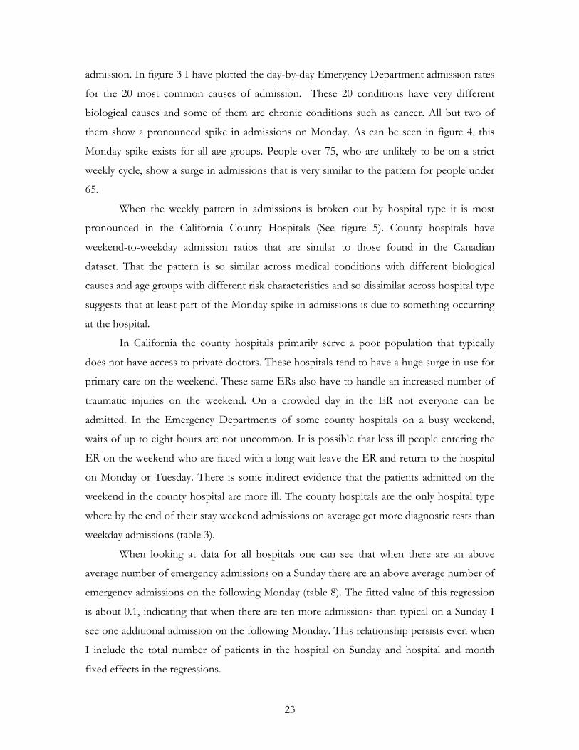
than their route into the hospital. A comparison of the proportion of patients admitted on
each day reveals that there are a disproportionate number of patients being admitted on
weekdays. In figure 1 I have plotted the proportion of the total admissions occurring on
different days of the week. It is immediately clear that there are a disproportionate number
5 If death during hospitalization is the outcome there are 6,676 deaths per 100,000 admissions on the weekend and 5,381 deaths per 100,000 admissions on weekdays. This difference is robust to the inclusion of covariates.
18

of admissions on weekdays. This pattern of disproportionate admissions during the week is
not caused by a few peculiar conditions. To examine this, I plot the weekend-to-weekday
admissions ratios for each of the top 100 causes of death. If there were no selection, for
every two patients entering the hospital on the weekend on average there would be five
patients entering the hospital on weekdays and we would expect the distributions should be
centered at 0.4. The admissions ratios for the top 100 causes of death are plotted in Figure 2.
The dotted line on the left of figure 2 is a kernel density estimate of the admissions ratios for
each of these causes of death. In examining the plots, it is immediately clear that all
conditions are showing a disproportionate number of weekday admissions.
Removing the voluntary hospital admissions by restricting the sample to patients
with unplanned admissions through the Emergency Department is the simplest way of
dealing with this problem. Dropping patients with voluntary admissions reduces my sample
size by 37.3%. Dropping these patients yields patients that have more similar demographics
as can be seen by comparing the first and second columns of table 1b with the third and
fourth. It also improves the admissions ratios. In figure 2 the kernel density estimate for
patients admitted through the Emergency Department is the solid line on the right. It is
centered just a little below the ratio 2:5 that we would expect if patients were entering the
hospital at random, showing that there are still slightly more weekday admissions for most
medical conditions. The improvement in the admissions ratios can also be seen by
comparing the proportions of patients admitted on different days. As can be seen in figure 1
the Emergency Department admissions are occurring much more randomly than the non-
emergency admissions.
When I make the weekday to weekend comparison using only patients with
unplanned admissions through the Emergency Department I find a small but statistically
significant difference in mortality rates between weekday and weekend admissions. The
mortality rate in the first day for weekday admissions is 1,611 per 100,000 patient days. The
mortality rate for weekend admissions is 1,650 per 100,000 patients days6. This difference of
39 deaths per 100,000 admissions is robust to the inclusion of covariates. As can be seen in
table 5 the inclusion of covariates in a logistic regression has almost no impact on the
estimate of the mortality differential between weekday and weekend admissions.
6 For all deaths within hospital there are 6,833 deaths per 100,000 admissions on the weekend and 6,766 deaths per 100,000 admissions on the weekend. This difference is robust to the inclusion of covariates.
19
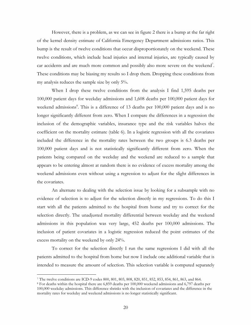
However, there is a problem, as we can see in figure 2 there is a bump at the far right
of the kernel density estimate of California Emergency Department admissions ratios. This
bump is the result of twelve conditions that occur disproportionately on the weekend. These
twelve conditions, which include head injuries and internal injuries, are typically caused by
car accidents and are much more common and possibly also more severe on the weekend7.
These conditions may be biasing my results so I drop them. Dropping these conditions from
my analysis reduces the sample size by only 5%.
When I drop these twelve conditions from the analysis I find 1,595 deaths per
100,000 patient days for weekday admissions and 1,608 deaths per 100,000 patient days for
weekend admissions8. This is a difference of 13 deaths per 100,000 patient days and is no
longer significantly different from zero. When I compare the differences in a regression the
inclusion of the demographic variables, insurance type and the risk variables halves the
coefficient on the mortality estimate (table 6). In a logistic regression with all the covariates
included the difference in the mortality rates between the two groups is 6.3 deaths per
100,000 patient days and is not statistically significantly different from zero. When the
patients being compared on the weekday and the weekend are reduced to a sample that
appears to be entering almost at random there is no evidence of excess mortality among the
weekend admissions even without using a regression to adjust for the slight differences in
the covariates.
An alternate to dealing with the selection issue by looking for a subsample with no
evidence of selection is to adjust for the selection directly in my regressions. To do this I
start with all the patients admitted to the hospital from home and try to correct for the
selection directly. The unadjusted mortality differential between weekday and the weekend
admissions in this population was very large, 452 deaths per 100,000 admissions. The
inclusion of patient covariates in a logistic regression reduced the point estimates of the
excess mortality on the weekend by only 24%.
To correct for the selection directly I run the same regressions I did with all the
patients admitted to the hospital from home but now I include one additional variable that is
intended to measure the amount of selection. This selection variable is computed separately
7 The twelve conditions are ICD-9 codes 800, 801, 803, 808, 820, 851, 852, 853, 854, 861, 863, and 864. 8 For deaths within the hospital there are 6,859 deaths per 100,000 weekend admissions and 6,797 deaths per 100,000 weekday admissions. This difference shrinks with the inclusion of covariates and the difference in the mortality rates for weekday and weekend admissions is no longer statistically significant.
20

for each condition. For each condition I calculate how far above 5/7 the proportion of
weekday admissions is. I do the same thing for weekend admissions. This gives me a variable
that characterizes the selection that takes on 200 different values, one for the weekend and
one for the weekdays for each of the 100 conditions included in the analysis. If the excess
patients admitted during the week are no different from the patients admitted on the
weekend then this variable should be orthogonal to the mortality rate and be
indistinguishable from zero.
When I run regressions with this selection variable included the strong evidence in
favor of excess mortality on the weekend disappears. Though the inclusion of all the
demographic variables has very little impact on the estimate of the mortality differential, the
inclusion of the selection variable in the regressions reduces the estimate of the mortality
differential by a factor of more than ten. As can be seen in last three columns of table 7,
when the selection variable is included in the regressions the large mortality difference on the
weekend shrinks to a number that is not distinguishable from zero. This is particularly
striking because as can be seen by looking at the first three columns of table 7 including
patient level covariates has very little impact on these estimates.
5.3 Reconciling my results with contradictory results from the literature
The two very different approaches to dealing with the selection problem – working
with a reduced subsample with little evidence of selection and correcting for the selection
directly – give us the same finding of no difference in mortality between the weekday and
the weekend. This finding is in contradiction with the findings of Bell and Redelmeier’s
paper from the New England Journal of Medicine (2001). They look at a Canadian dataset
and find that for 23 of the top 100 causes of death there is excess mortality for patients
admitted through the Emergency Department on the weekend and there are no conditions
for which they find excess mortality for patients admitted on weekdays. There are a number
of reasons to be skeptical about their findings. Thirteen of the conditions for which they are
finding evidence of excess mortality are cancers; it is surprising that outcomes for these
conditions are so sensitive to short term variation in the quality of care. Their data also
shows significant evidence of selection. As can be seen in figure 2 the kernel density estimate
of the admissions ratios for the Canadian dataset (denoted by the long dashed line) shows
21

that for almost every condition there are far more admissions occurring on weekdays than
we would expect if people were entering the hospital at random. In the Canadian dataset all
but one of the conditions has a disproportionate share of admissions during the week. This
bias in favor of weekday admissions needs to be examined closely. If there are systematic
differences between patients entering the hospital on different days Bell and Redelmeier’s
results may reflect selection rather than a reduction in the quality of care people are receiving
on the weekend.
Since the Canadian study is focused on just Emergency Department admissions and
none of the conditions with excess mortality are accidental admissions, neither of the two
types of selection I discussed above could be driving the result. This leads me to look for
evidence of the third kind of selection mentioned above: hospital triage. Though I cannot
examine the Canadian data directly, I can look for evidence of hospital triage in California.
When we examine the kernel density estimates of hospital admissions in figure 2 it is
clear that the estimate for California Emergency Department admissions lies a little to the
left of the 0.4 ratio, indicating that most conditions have a disproportionate number of
admissions on weekdays. The excess admissions on weekdays in California for patients
admitted through the Emergency Department are due almost entirely to a surge in
admissions on Monday. As can be seen in figure 1 there are 7.3% more admissions on
Monday than we would expect if people were coming in at random.
5.4 The evidence of hospital triage in California
The surge in heart attacks reported on Mondays is well documented in the medical
literature but the mechanism is unclear. A recent study by Evans et al (British Medical
Journal 2000) suggests that increased alcohol consumption on the weekend is a possible
cause. Chenet et al observe that the surge in Monday heart attacks does not occur for
people with a previous admission for coronary heart disease and suggest that it is possible
that either they are protected by their existing therapy plan or they are more likely to seek
treatment on the weekend. Peters et al (Circulation 1996) find a pattern in heart attacks for
all population subtypes except patients on Beta-Blockers.
There is little evidence on septadian patterns for medical conditions other than heart
attacks. In California there is a surge in Monday admissions for almost every cause of
22
admission. In figure 3 I have plotted the day-by-day Emergency Department admission rates
for the 20 most common causes of admission. These 20 conditions have very different
biological causes and some of them are chronic conditions such as cancer. All but two of
them show a pronounced spike in admissions on Monday. As can be seen in figure 4, this
Monday spike exists for all age groups. People over 75, who are unlikely to be on a strict
weekly cycle, show a surge in admissions that is very similar to the pattern for people under
65.
When the weekly pattern in admissions is broken out by hospital type it is most
pronounced in the California County Hospitals (See figure 5). County hospitals have
weekend-to-weekday admission ratios that are similar to those found in the Canadian
dataset. That the pattern is so similar across medical conditions with different biological
causes and age groups with different risk characteristics and so dissimilar across hospital type
suggests that at least part of the Monday spike in admissions is due to something occurring
at the hospital.
In California the county hospitals primarily serve a poor population that typically
does not have access to private doctors. These hospitals tend to have a huge surge in use for
primary care on the weekend. These same ERs also have to handle an increased number of
traumatic injuries on the weekend. On a crowded day in the ER not everyone can be
admitted. In the Emergency Departments of some county hospitals on a busy weekend,
waits of up to eight hours are not uncommon. It is possible that less ill people entering the
ER on the weekend who are faced with a long wait leave the ER and return to the hospital
on Monday or Tuesday. There is some indirect evidence that the patients admitted on the
weekend in the county hospital are more ill. The county hospitals are the only hospital type
where by the end of their stay weekend admissions on average get more diagnostic tests than
weekday admissions (table 3).
When looking at data for all hospitals one can see that when there are an above
average number of emergency admissions on a Sunday there are an above average number of
emergency admissions on the following Monday (table 8). The fitted value of this regression
is about 0.1, indicating that when there are ten more admissions than typical on a Sunday I
see one additional admission on the following Monday. This relationship persists even when
I include the total number of patients in the hospital on Sunday and hospital and month
fixed effects in the regressions.
23

5.5 The relationship between triage and excess mortality on the weekend
It is important to determine if the amount of triage evident for a given condition is
related to the mortality rate for that condition. When the conditions are broken out into
three groups based on the mortality differential between the weekday and weekend
admissions there is a clear pattern. Figure 6 shows the weekly pattern in admissions for
conditions by how much evidence of excess mortality there is for the condition. The more
evidence of excess mortality there is for the condition the more pronounced the spike in
Monday admissions. For the 30 conditions with the least evidence of excess mortality there
are a 6.3% more admissions than we would expect on Monday than if the admissions were
occurring at random. For the 30 conditions with the most evidence of excess mortality on
the weekend there are 11.8% more admissions on Monday than we would expect if they
were occurring at random. This clear association between the Monday spike and the amount
of excess mortality on the weekend is probably driving the slight and statistically insignificant
difference in the mortality rates between the weekday and the weekend that I am finding in
the California hospitals.
The patients entering the Emergency Department in Canada are more ill and are in
general more likely to enter the hospital on a weekday than the patients entering California
Emergency Departments. Canadian Emergency Departments have higher mortality rates for
every condition. In figure 7 I have plotted the mortality rate for Emergency Department
admissions in Canada against the mortality rate in California condition by condition. The
patients entering the hospital through the Emergency Department in Canada are clearly
higher risk than the patients entering the hospital through the Emergency Department in
California. Figure 8 plots the admissions ratios in California against the admissions ratios in
Canada. Conditions that have more weekday admissions than we would expect in California
also have more weekday admissions than we would expect in Canada. The mechanism that is
causing the excess weekday admissions in Canada appears to be operating in a fashion
similar to the mechanism in California. However in Canada for most conditions the selection
is much more pronounced.
When I examine the relationship between the admissions ratios and the evidence of
excess mortality on the weekend in the Canadian dataset the results are striking. Figure 9
24

plots the ratio of weekend to weekday admissions against the differences the mortality rates
for the Canadian dataset. The solid circles denote individual conditions for which Bell and
Redelmeier found significant evidence of excess mortality on the weekend. The relationship
between the amount of sorting and the amount of mortality on the weekend is striking.
Conditions with the most excess admissions on weekdays have the most evidence of excess
mortality on the weekend. This significant relationship between the amount of sorting and
the mortality rates probably reflects triage in the Emergency Department. If only the sickest
patients are admitted to the hospital on the weekend the patients admitted on the weekend
will have a higher mortality rate than the patient population in general. For a given condition
the more triage there is the greater the difference in mortality rates between the weekday and
the weekend admissions. In the next section I will try three ways of dealing with the bias
introduced by the disproportionate number of weekday admissions in the Canadian dataset.
Since the patient level data is unavailable I will work with the data at the level of the
condition.
5.6 Three ways of correcting for the selection in the Canadian data
In this section I implement three different ways of correcting for the association
between the admissions rate and the mortality rate documented above. I do not have access
to the patient level data so I am unable to estimate models with covariates. Instead I take
advantage of the admissions ratios which provide me with a direct measure of the amount of
selection that is occurring.
The most conservative way to proceed is to assume that all the additional people
appearing during the week are surviving and to re-estimate the odds ratios under this
assumption. From an estimation perspective this is the worst case scenario and would create
a large bias in estimates of the excess mortality on the weekend in Canada. I can put a lower
bound on the mortality estimates by assuming none of the people who deferred coming in
until a weekday died and reassign them back to the weekend. When I do this not one of the
23 conditions that showed evidence of excess mortality on the weekend in the Canadian
dataset still does. This is probably overly pessimistic as some of the people that defer
entering the hospital probably die.
25

An alternative is to estimate the mortality rate for conditions that show no evidence
of selection. There are nine conditions that have weekend-to-weekday admissions ratios that
are not statistically different from 2/7. These nine conditions account for 267,775
admissions. The weekday mortality rate in this group is 4.83%. The weekend mortality rate
is 4.63%. This approach reveals no evidence in favor of excess mortality on the weekend but
is limited in power due to the reduced sample size.
An alternate approach that works with the entire sample and corrects for the bias
instead of estimating a lower bound is to run a regression that corrects for the bias using the
method developed above. I start with an estimate of the difference in the mortality rate
between the weekend and weekdays.
- Weekend Weekday mortality condition c τ=
This gives me an estimateτ of .00534 which is statistically significantly different from
zero (Column 1 of table 9). This is equivalent to an additional 524 deaths per 100,000
admissions. If there were no selection this would be an unbiased estimate of the weekend
treatment effect.
Since I am finding clear evidence of selection in figure 9 I need to take steps to
correct for it. I implement two different strategies. In the first approach I assume that the
patients who defer coming in until a weekday are dying at a constant fraction of the
mortality rate for people admitted on the weekend. This makes it possible to estimate τ
while adjusting for the bias. In this equation α is the percent of patients that defer coming in
and is the weekend mortality rate for condition c.
B
c
Mec9
7 Mec5 2
- (1 ) cc
Weekend Weekday mortality condition c B αα
τ+
= + −
When I run this regression I get an estimate of and of and .59 and -0.00121
respectively. The estimate of τ is not statistically different from zero (Column 2 of table 9).
This suggests that even if the patients who deferred coming in were dying at only 60% of the
rate of patients that came in on the weekend it would explain away the entire difference in
mortality between the weekend and the weekdays. An alternative way of correcting for the
selection that makes no assumptions about the mortality rate of the additional patients that
are deferring entering the hospital would be to compare the mortality rate of weekend
admissions with the mortality rate of weekday admissions, adjusting for the cross over rate,
B τ
9 The motivation for this equation was presented in the methods section
26

cα , and the square of the cross over rate α . If the mortality difference between the
weekend and weekdays is not being driven by some characteristic of the patients who are
deferring entering the hospital then it should be unaffected by including a measure of the
number of patients crossing over for each condition. The equation that I estimate is.
2c
ort 2 - c cWeekend Weekday m ality condition c τ α α= + +
This regression reveals a mortality differential between the weekday and the weekend
of –0.00015 which is not significantly different from zero (Column 3 of table 9).
Though the patients admitted during the weekday and the weekend in the Canadian
dataset have very similar observable characteristics and Bell and Redelmeier’s results were
robust to the inclusion of covariates, there is a serious problem with selection on
unobservable characteristics. The four different approaches above all found no evidence in
support of excess mortality on the weekend. There appears to be a significantly less ill
subpopulation that is deferring entering the hospital until a weekday. This subpopulation
appears to be driving the differences in the mortality rate documented in the paper by Bell
and Redelmeier.10
6. Conclusions
I find no evidence of excess mortality on the weekend in the California hospital
system for people admitted through the Emergency Department. This is despite a significant
delay in diagnostic and treatment procedures for patients admitted on the weekend. The
research design I implemented above has the rare property that the selection is observable.
This makes it possible to examine the impact of relatively small amounts of selection on the
results. I find that even a small amount of selection can generate statistically significant
spurious results that are robust to the inclusion of covariates that are typically available in
hospital discharge datasets. The one published study that found evidence of excess mortality
10 Bell and Redelmeier also find evidence of excess mortality for three conditions they expect to be particularly vulnerable to a reduction in care. These conditions are abdominal aortic aneurysm, acute epiglottitis and pulmonary embolism. There is no evidence of excess mortality on the weekend for these conditions in California even without adjusting for covariates. The admissions ratios for these three conditions in the Canadian dataset are .322, .462 and .292 respectively. The ratios in California are much closer to .4 they are .365, .439 and .365 respectively. (Table available on request)
27

among patients admitted through the Emergency Department on the weekend appears to be
documenting a spurious result due to selection caused by hospital triage.
This study reveals that, even when the covariates of the patients being compared are
much closer than in the across-hospital comparisons typical in the literature, selection can
still be a serious problem. Even when the comparison is being made within-hospital so that
fixed differences between hospitals are not a problem, doctor’s and patient’s responses to
scarce resources can have a confounding effect. The patients who have the scarce resources
available on the weekend allocated to them are more ill on average than the patients entering
the hospital on other days of the week. In a setting where the allocation of scarce resources
results in a significant amount of selection and the selection is unrecognized, it can create the
appearance of a positive relationship between the resources available and patient’s outcomes.
Hospitals have rational motives to reduce staffing on the weekend. The social cost of
maintaining a constant staffing level is higher on the weekend. Hospital staff that is required
to work on the weekend is forced to give up time they could spend with their families. The
hospitals have responded by reducing the staffing and services provided on the weekend.
This reduction in staffing has two effects. Some patients, particularly at county hospitals, are
unable to enter the hospital on the weekend and have to defer coming in until Monday. The
patients who are admitted to the hospital on the weekend are receiving fewer services in the
first few days after they enter the hospital. The hospital staff appears to be doing a good job
of allocating the relatively scarce resources on the weekend because there is no evidence that
the temporary reduction in services is resulting in a higher probability of dying for patients
admitted on the weekend.
What this study tells us about the relationship between staffing and mortality is more
limited. That a short term reduction in the ratio of doctors to patients is not resulting in a
higher mortality rate among patients suggests that there is no strong relationship between
the number of doctors on site and the probability that an error that will results in a patients
dying will occur. However this does not tell us what would occur if staffing levels were
permanently reduced. A permanent reduction in staff to the weekend level would be unable
to handle the influx of additional patients that occurs on Monday and also would not be able
to provide all the additional procedures that were deferred for patients that entered the
hospital on the weekend.
28

Bibliography Daily Variation in USA Morality. Am J Epidemiol 1976, 103:198-211 Aiken L., Clarke S., Sloane D., Sochalski J., and Silber J. Hospital Nurse Staffing and Patient Mortality, Nurse Burnout, and Job Dissatisfaction. JAMA 2002;288:161987-1993 Asch D., Parker R. Sounding Board: The Libby Zion Case. N England J Med, March 24, 1988 Vol. 318 No.12 Bell C. M., Redelmeier D. A. Mortality Among Patients Admitted to Hospitals on Weekends as Compared With Weekdays. N England J Med, Vol. 345, no. 9 August 30 2001 Blegen M., Goode C., Reed L. Nurse Staffing and Patient Outcomes. Nursing Research January/February 1998 Vol 47, No Chenet L., Britton A., Kalediene R., and Petrauskiene J. Daily Variations in Deaths in Lithuania: The Possible Contribution of Binge Drinking, Int. J. Epidemiol. 30: 743-748 Czaplinski C, Diers D. The Effect of Staff Nursing on Length of Stay and Mortality. Medical Care Vol. 36, No. 12 pp 1626-1683 Dowding V., Duignan N., Henry G., MacDonald. Induction of Labour, Birthweight and Perinatal mortality by day of the week. British Journal of Obstetrics and Gynecology Evans C., Chalmers J., Capewell S. et al "I don't like Mondays"--Day of the Week of Coronary Disease Deaths in Scotland: Study of Routinely Collected Data. BMJ Vol 320 22 January 2000 Fielding L. P., Stewart-Brown S. and Blesovsky. Large Bowel Obstruction Caused by Cancer: A Prospective Study. British Medical Journal 2, 515, 1979 Fogelholm R, Murros K, Rissanen A, Ilmavirta M. Factors Delaying Hospital Admission After Acute Stroke. Stroke 1996 Mar;27(3):398-400 Gottlieb DJ, Parenti CM, Peterson CA, Lofgren RP. Effect of a Change in House Staff Work Schedule on Resource Utilization and Patient Care. Arch Intern Med. 1991 Oct;151(10):2065-70. Hartz AJ, Krakauer H, Kuhn Em, et al. Hospital characteristics and mortality rates. N Engl J Med 1989;321-1720-5 Hendry R. A. The Weekend-- A Dangerous Time to be Born?. Br. J. Obstet Gynaecol. 88, 1200 1981 Kohn L.T., Corrigan J.M., Donaldson M., eds. To Err is Human: Building a Safer Health System. Washington, DC: Institute of Medicine; 1999 Lamn H. The Lost Weekend in Hospitals. N Engl J Med, 1973; 289:923 Leape L. Institute of Medicine Medical Error Figures are Not Exaggerated. JAMA, Vol. 284, no. 1 July 5 2000 Mathers C. Births and perinatal deaths in Australia: Variations by Day of week. Journal of Epidemiology and Community Health, 1983, 37, 57-62 McDonald C., Weiner M., and Hui S. P. Deaths Due to Medical Errors are Exaggerated in Institute of Medicine Report. JAMA, Vol. 284, no. 1 July 5 2000 McFarlane A. Variations in the Number of Births and Perinatal Mortality by Day of the Week in England and Wales. Br. Med J. 2, 1970, 1978
29

McKee M, Black N. Does the Current Use of Junior Doctors in the United Kingdom Affect the Quality of Medical Care?. Soc Sci Med. 1992 Mar;34(5):549-58 Needleman J, Buerhaus P, Mattke S, Stewart M, Zelevinsky. Nurse-Staffing Levels and the Quality of Care in Hospitals. N Engl J Med, Vol. 346, No. 22 May 30 2002 Peters RW, McQuillan S, Resnick SK, Gold M. Increased Monday Incidence of Life-Threatening Ventricular Arrhythmias. Circulation 1996;94:1346-1349 Pronovost PJ, Jenkes MW, Dorman T, et al. Organization Characteristics of Intensive Care Units Related to Outcomes of Abdominal Aortic Surgery. JAMA 1999;281:1310-7 Silber JH, Rosenbaum PR, Schwartz JS, Ross RN, Williams SV. Evaluation of the Complication Rate as a Measure of Quality of Care in Coronary Artery Bypass Graft Surgery. JAMA 1995:274:317-23 Silber JH, Rosenbaum PR. A Spurious Correlation Between Hospital Mortality and Complication Rates: The Importance of Severity Adjustment.. Med Care 1997:35:Suppl:OS77-OS92 Spence M. T., Redmond A.D. and Edwards J. D. Trauma Audit -- The use of TRISS. Hlth Trends 3, 94, 1988 Tarnow-Mordi WO, Hau C, Warden A, Shearer AJ. Hospital Mortality in Relation to Staff Workload: A 4-Year Study in an Adult Intensive-Care Unit. Lancet. 2000 Jul 15;356(9225):185-9. Thorpe KE. House Staff Supervision and Working Hours. Implications of Regulatory Change in New York State. JAMA. 1990 Jun 20;263(23):3177-81
30
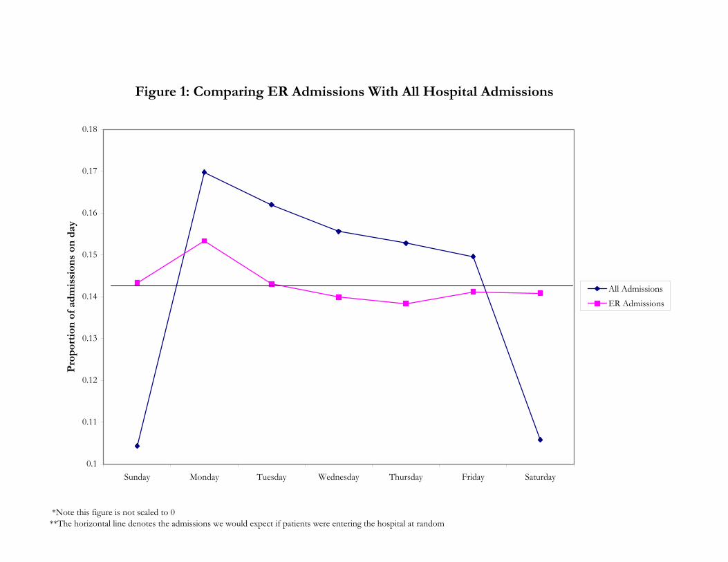
*Note this figure is not scaled to 0 **The horizontal line denotes the admissions we would expect if patients were entering the hospital at random
Figure 1: Comparing ER Admissions With All Hospital Admissions
0.1
0.11
0.12
0.13
0.14
0.15
0.16
0.17
0.18
Sunday Monday Tuesday Wednesday Thursday Friday Saturday
Pro
por
tion
of
adm
issi
ons
on d
ay
All AdmissionsER Admissions

0.0 0.1 0.2 0.3 0.4 0.5 0.6 0.7Weekend admissions / Weekday admissions
0.00
5.00
10.00
15.00
20.00
f(x)
Figure 2: Hospital Admission Ratios California vs Canada (Top 100 Causes of Death)
Dots: All admissions from home CaliforniaDashed: All admissions through ER CanadaSolid: All admissions through ER California

*Note this figure is not scaled to 0 **Most other causes of admissions show a similar spike on Mondays with the exception of external causes which peak on the weekend.
Figure 3: Weekly Patterns for the Top 20 Causes of Hospital Admission
0.1
0.11
0.12
0.13
0.14
0.15
0.16
0.17
0.18
Sunday Monday Tuesday Wednesday Thursday Friday Saturday
Pro
por
tion
of
adm
issi
ons
on d
ay
*Note this figure is not scaled to 0 **These admission patterns are for the emergency room admissions that are the 100 top causes of death
Figure 4: Daily Admission Cycle by Age
0.1
0.11
0.12
0.13
0.14
0.15
0.16
0.17
0.18
Sunday Monday Tuesday Wednesday Thursday Friday Saturday
Pro
por
tion
of
adm
issi
ons
on d
ay
Age to 26-35Age 36 to 45Age 46 to 55Age 56 to 65Age 66 to 75Age 76 to 85Age 86 to 95

*Note the chart is not scaled to 0**These charts are generated using all California Emergency Room admissions for each hospital type
Figure 5: Hospital Admissions by Hospital Type
0.1
0.11
0.12
0.13
0.14
0.15
0.16
0.17
0.18
Sunday Monday Tuesday Wednesday Thursday Friday Saturday
Prop
ortio
n of
adm
issio
ns o
n a
day
County HospitalNonprofit HospitalStaff Model HMOChurch HospitalFor Profit Hospital

*The top 100 Causes of death are broken up into three even groups based on how much evidence of excess mortality there is among weekend admissions.
Figure 6: California ER Daily Admission Rates by Excess Mortality Rate
0.1
0.11
0.12
0.13
0.14
0.15
0.16
0.17
0.18
Sunday Monday Tuesday Wednesday Thursday Friday Saturday
Pro
por
tion
of
adm
issi
ons
on d
ay
No excess mortality on theweekendSome excess mortality onthe weekendMost excess mortality onthe weekend

*Mortality rates are for the entire hospitalization **The mortality rates are for the 73 conditions that are among the top 100 causes of death in both datasets
Figure 7: Mortality Rates for Californian vs Canadian ER Admissions
0%
10%
20%
30%
40%
50%
60%
0% 10% 20% 30% 40% 50% 60%
California: Mortality rate entire hospitalization
Can
ada:
Mor
talit
y ra
te e
nti
re h
osp
ital
izat
ion

0.20 0.25 0.30 0.35 0.40 0.45 0.50California: Weekend admissions/ Weekday admissions
0.20
0.25
0.30
0.35
0.40
0.45
0.50
Cana
da: W
eeke
nd a
dmiss
ions
/ W
eekd
ay a
dmiss
ions
Figure 8: Differences in Admission Ratios

0.20 0.25 0.30 0.35 0.40 0.45 0.50Weekend admissions/Weekday admissions
-0.05
0.00
0.05
0.10
Wee
kend
- W
eekd
ay m
orta
lity
rate
sFigure 9: Bell and Redelmeier Results Top 95 Non-Trauma Conditions
Squares = Not Statistically Significant
Circles = Statistically Signficant Excess Mortality on the Weekend

LargestSecond Largest Largest
Second Largest Largest
Second Largest Largest
Second Largest
Length of Stay (first admission) 5.50 4.37 6.14 4.54 3.96 4.40 5.73 5.35Age of Patient 58.70 61.40 61.79 65.58 66.69 60.88 39.80 41.39Percent male 49.19% 49.24% 48.15% 44.16% 44.12% 44.50% 52.57% 46.42%Percent White 88.24% 95.01% 75.20% 90.90% 89.84% 91.77% 35.11% 26.39%Percent Black 3.26% 1.11% 16.27% 4.12% 1.47% 4.39% 15.28% 22.11%Percent Asian 1.63% 3.05% 2.97% 3.06% 0.31% 2.12% 5.70% 7.95%Percent Hispanic 13.67% 7.86% 6.25% 12.47% 7.39% 6.10% 66.76% 57.05%Description of condition Counts of diagnosis 5.69 4.86 4.83 5.76 4.04 5.46 2.55 2.50 Counts of procedures 1.69 1.79 0.71 0.93 1.25 0.66 0.67 0.57 Injury due to external causes 23.34% 23.41% 17.20% 15.42% 13.16% 17.97% 25.06% 13.06%Insurance type Medicare 45.90% 38.34% 49.12% 64.83% 72.07% 51.36% 4.90% 8.24% HMO 12.61% 31.75% 13.11% 7.42% 5.83% 11.14% 0.53% 0.20% Medi-Cal 17.03% 4.21% 11.07% 10.07% 11.76% 16.38% 48.29% 44.87% PPO 12.52% 15.31% 13.68% 11.55% 2.01% 4.56% 0.01% 0.11% Private 4.36% 2.68% 3.19% 3.36% 3.20% 6.31% 1.28% 2.87% Self Pay 2.69% 2.91% 7.97% 2.13% 2.94% 4.29% 17.66% 0.18% County Indigent 3.73% 3.81% 0.01% 0.03% 1.19% 4.86% 19.22% 38.74% Other Government 0.20% 0.38% 1.21% 0.03% 0.11% 0.55% 7.49% 4.33% Workers comp 0.91% 0.53% 0.43% 0.59% 0.89% 0.53% 0.59% 0.43% Other payer 0.05% 0.06% 0.16% 0.00% 0.00% 0.00% 0.02% 0.02% Unknown 0.00% 0.00% 0.04% 0.00% 0.01% 0.01% 0.00% 0.00%Total admissions 26,445 26,662 58,675 41,238 42,593 37,366 176,133 78,771*The demographics are for all admissions for the top 100 causes of death between 1995 and 1999
Table 1a: Patient Demographics for the Two Largest Hospitals of Each Type in California
Private Proprietary Private Nonprofit District County
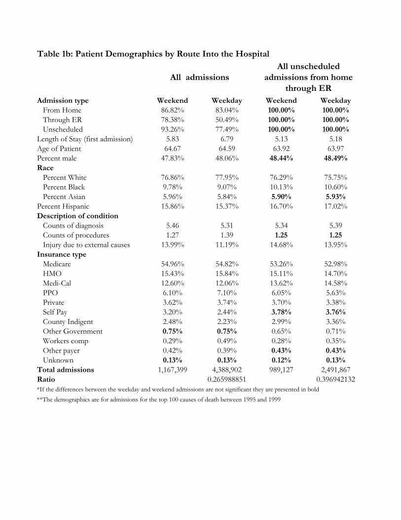
Admission type Weekend Weekday Weekend Weekday From Home 86.82% 83.04% 100.00% 100.00% Through ER 78.38% 50.49% 100.00% 100.00% Unscheduled 93.26% 77.49% 100.00% 100.00%Length of Stay (first admission) 5.83 6.79 5.13 5.18Age of Patient 64.67 64.59 63.92 63.97Percent male 47.83% 48.06% 48.44% 48.49%Race Percent White 76.86% 77.95% 76.29% 75.75% Percent Black 9.78% 9.07% 10.13% 10.60% Percent Asian 5.96% 5.84% 5.90% 5.93%Percent Hispanic 15.86% 15.37% 16.70% 17.02%Description of condition Counts of diagnosis 5.46 5.31 5.34 5.39 Counts of procedures 1.27 1.39 1.25 1.25 Injury due to external causes 13.99% 11.19% 14.68% 13.95%Insurance type Medicare 54.96% 54.82% 53.26% 52.98% HMO 15.43% 15.84% 15.11% 14.70% Medi-Cal 12.60% 12.06% 13.62% 14.58% PPO 6.10% 7.10% 6.05% 5.63% Private 3.62% 3.74% 3.70% 3.38% Self Pay 3.20% 2.44% 3.78% 3.76% County Indigent 2.48% 2.23% 2.99% 3.36% Other Government 0.75% 0.75% 0.65% 0.71% Workers comp 0.29% 0.49% 0.28% 0.35% Other payer 0.42% 0.39% 0.43% 0.43% Unknown 0.13% 0.13% 0.12% 0.13%Total admissions 1,167,399 4,388,902 989,127 2,491,867Ratio 0.265988851 0.396942132
**The demographics are for admissions for the top 100 causes of death between 1995 and 1999
Table 1b: Patient Demographics by Route Into the Hospital
All admissionsAll unscheduled
admissions from home through ER
*If the differences between the weekday and weekend admissions are not significant they are presented in bold

Table 1c: Percent of Patients Admitted to Nearest Hospital
Planned Admissions
Emergency Room
AdmissionsAll Admissions 21.95% 31.35%Race Black 14.45% 21.31% White 23.39% 33.88%Insurance type Medi-Cal 19.07% 27.62% Medicare 25.35% 35.49% HMO 16.80% 24.13% PPO 19.25% 30.93% Private 21.10% 33.38%
*Distance from residence to hospital to is calculated using the population centroid of the residential zip code and the exact location of the hospital. It was not possible to calculate a distance for 2% of the admissions due to missing residential zip code. The numbers presented above are for all admissions from home between 1995-1999
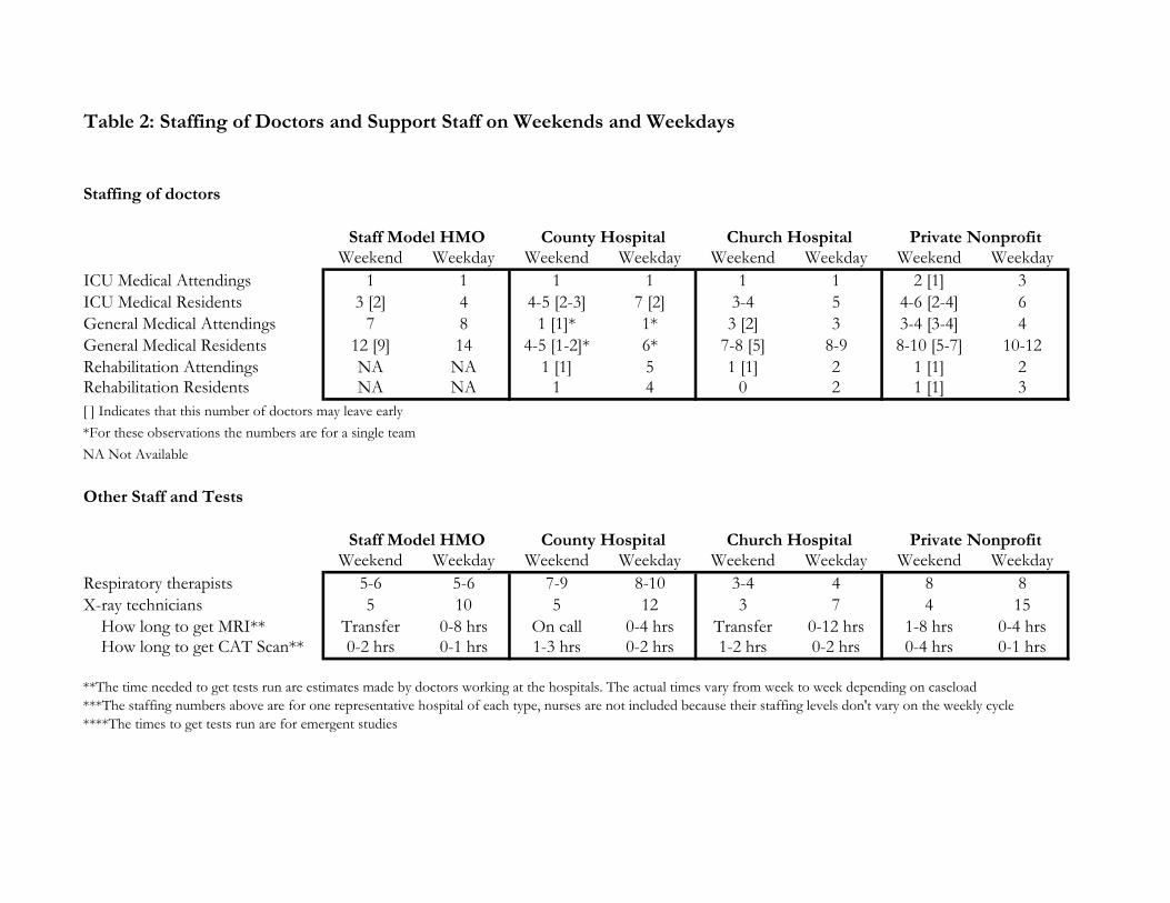
Table 2: Staffing of Doctors and Support Staff on Weekends and Weekdays
Staffing of doctors
Weekend Weekday Weekend Weekday Weekend Weekday Weekend WeekdayICU Medical Attendings 1 1 1 1 1 1 2 [1] 3ICU Medical Residents 3 [2] 4 4-5 [2-3] 7 [2] 3-4 5 4-6 [2-4] 6General Medical Attendings 7 8 1 [1]* 1* 3 [2] 3 3-4 [3-4] 4General Medical Residents 12 [9] 14 4-5 [1-2]* 6* 7-8 [5] 8-9 8-10 [5-7] 10-12Rehabilitation Attendings NA NA 1 [1] 5 1 [1] 2 1 [1] 2Rehabilitation Residents NA NA 1 4 0 2 1 [1] 3[ ] Indicates that this number of doctors may leave early*For these observations the numbers are for a single teamNA Not Available
Other Staff and Tests
Weekend Weekday Weekend Weekday Weekend Weekday Weekend WeekdayRespiratory therapists 5-6 5-6 7-9 8-10 3-4 4 8 8X-ray technicians 5 10 5 12 3 7 4 15 How long to get MRI** Transfer 0-8 hrs On call 0-4 hrs Transfer 0-12 hrs 1-8 hrs 0-4 hrs How long to get CAT Scan** 0-2 hrs 0-1 hrs 1-3 hrs 0-2 hrs 1-2 hrs 0-2 hrs 0-4 hrs 0-1 hrs
**The time needed to get tests run are estimates made by doctors working at the hospitals. The actual times vary from week to week depending on caseload***The staffing numbers above are for one representative hospital of each type, nurses are not included because their staffing levels don't vary on the weekly cycle****The times to get tests run are for emergent studies
Private Nonprofit
Staff Model HMO County Hospital Private NonprofitChurch Hospital
Staff Model HMO County Hospital Church Hospital

Table 3: Procedures Performed After Admission Through the ER
Weekend Weekday DifferenceDiagnostic Procedures
First Day 0.513 0.547 6.68%First Two days 0.723 0.793 9.70%During admission 1.183 1.188 0.39%
All ProceduresFirst Day 0.664 0.721 8.62%First Two days 0.996 1.119 12.37%During admission 1.838 1.862 1.32%
Observations 967,034 2,450,087*This is for inpatient admissions for internal causes in California 1995-1999
Weekend Weekday Difference Weekend Weekday DifferenceDiagnostic Procedures
First Day 0.504 0.546 8.33% 0.544 0.550 0.97%First Two days 0.722 0.816 13.06% 0.696 0.725 4.26%During admission 1.221 1.224 0.28% 1.100 1.080 -1.82%
All ProceduresFirst Day 0.637 0.699 9.81% 0.702 0.726 3.34%First Two days 0.961 1.103 14.77% 0.949 1.019 7.40%During admission 1.725 1.749 1.38% 1.716 1.720 0.25%
Observations 109,401 288,956 64,590 185,518
Weekend Weekday Difference Weekend Weekday DifferenceDiagnostic Procedures
First Day 0.409 0.447 9.20% 0.506 0.542 7.27%First Two days 0.608 0.686 12.70% 0.725 0.798 10.09%During admission 1.073 1.079 0.56% 1.195 1.205 0.82%
All ProceduresFirst Day 0.556 0.620 11.65% 0.653 0.714 9.33%First Two days 0.890 1.027 15.38% 0.999 1.131 13.17%During admission 1.792 1.818 1.46% 1.876 1.908 1.67%
Observations 142,434 353,742 374,825 930,233**These are for admissions due to internal causes for all hospitals each type
Church Hospitals** Private Nonprofit**
County Hospitals**
All Hospitals*
Staff Model HMO**

Table 4: All Patients Admitted From Home*
(1) (2) (3)Weekend Admission 0.346 0.269 0.262
[0.009] [0.009] [0.009]Male 0.173 0.165
[0.008] [0.008]Age 18-40 0.167 0.144
[0.042] [0.042]Age 40-50 0.122 0.127
[0.042] [0.042]Age 50-60 0.154 0.173
[0.041] [0.041]Age 60-70 0.265 0.345
[0.040] [0.041]Age 70-80 0.421 0.552
[0.040] [0.041]Age > 80 0.863 0.998
[0.040] [0.040]Black -0.195 -0.187
[0.016] [0.016]Asian 0.062 0.047
[0.016] [0.017]Hispanic -0.074 -0.087
[0.012] [0.012]External -0.261 -0.273
[0.013] [0.013]1996 0.193 0.196
[0.013] [0.013]1997 0.093 0.096
[0.013] [0.013]1998 0.053 0.055
[0.013] [0.013]1999 0.023 0.029
[0.013] [0.013]Severity 1.76 1.759
[0.006] [0.006]Constant -4.489 -5.87 -6.023
[0.005] [0.040] [0.041]Dummies for Insurance type No No YesObservations 5,556,301 5,556,301 5,556,301Robust standard errors in brackets, the dependent variable is mortality in the first day after admission*These are logistic regression run on all patients who arrived from home including 2,075,307 planned admissions

Table 5: Emergency Room Admissions*
(1) (2) (3)Weekend Admission 0.024 0.025 0.022
[0.009] [0.010] [0.010]Male 0.171 0.161
[0.009] [0.009]Age 18-40 0.046 0.030
[0.047] [0.047]Age 40-50 -0.016 -0.010
[0.047] [0.047]Age 50-60 0.010 0.020
[0.046] [0.046]Age 60-70 0.118 0.179
[0.045] [0.045]Age 70-80 0.268 0.376
[0.045] [0.045]Age > 80 0.655 0.769
[0.044] [0.045]Black -0.266 -0.244
[0.017] [0.017]Asian 0.067 0.069
[0.018] [0.018]Hispanic -0.095 -0.091
[0.013] [0.013]External -0.300 -0.313
[0.014] [0.014]1996 0.167 0.169
[0.014] [0.014]1997 0.055 0.056
[0.014] [0.014]1998 0.007 0.009
[0.014] [0.014]1999 -0.032 -0.026
[0.014] [0.014]Severity 1.681 1.681
[0.007] [0.007]Constant -4.111 -5.317 -5.450
[0.005] [0.045] [0.046]Dummies for Insurance type No No YesObservations 3,480,994 3,480,994 3,480,994Robust standard errors in brackets, the dependent variable is mortality in the first day after admission*These are logistic regression run on all patients who are admitted through the ER and arrived from home

Table 6: All Admissions Through the Emergency Room (Internal Causes)
(1) (2) (3)Weekend Admission 0.008 0.007 0.004
[0.010] [0.010] [0.010]Male 0.115 0.108
[0.009] [0.009]Age 18-40 0.795 0.796
[0.089] [0.089]Age 40-50 1.102 1.107
[0.088] [0.088]Age 50-60 1.164 1.163
[0.088] [0.088]Age 60-70 1.294 1.328
[0.087] [0.088]Age 70-80 1.455 1.524
[0.087] [0.088]Age > 80 1.852 1.925
[0.087] [0.087]Black -0.283 -0.262
[0.018] [0.018]Asian 0.033 0.043
[0.019] [0.019]Hispanic -0.143 -0.127
[0.014] [0.014]External -0.762 -0.762
[0.020] [0.020]1996 0.171 0.172
[0.015] [0.015]1997 0.059 0.060
[0.015] [0.015]1998 0.010 0.010
[0.015] [0.015]1999 -0.027 -0.023
[0.015] [0.015]Severity 1.677 1.676
[0.007] [0.007]Constant -4.122 -6.425 -6.516
[0.005] [0.087] [0.088]Dummies for Insurance type No No YesObservations 3,302,360 3,302,360 3,302,360Robust standard errors in brackets, the dependent variable is mortality in the first day after admission*These are logistic regression run on ER admissions due to causes identified as internal based on ICD-9

Table 7: All Patients Admitted From Home
(1) (2) (3) (4) (5) (6)Weekend Admission 0.346 0.269 0.262 -0.057 -0.021 -0.025
[0.009] [0.009] [0.009] [0.019] [0.019] [0.019]Male 0.173 0.165 0.174 0.165
[0.008] [0.008] [0.008] [0.008]Age 18-40 0.167 0.144 0.168 0.146
[0.042] [0.042] [0.042] [0.042]Age 40-50 0.122 0.127 0.122 0.127
[0.042] [0.042] [0.042] [0.042]Age 50-60 0.154 0.173 0.156 0.174
[0.041] [0.041] [0.041] [0.041]Age 60-70 0.265 0.345 0.267 0.347
[0.040] [0.041] [0.040] [0.041]Age 70-80 0.421 0.552 0.422 0.553
[0.040] [0.041] [0.040] [0.041]Age > 80 0.863 0.998 0.859 0.994
[0.040] [0.040] [0.040] [0.041]Black -0.195 -0.187 -0.200 -0.191
[0.016] [0.016] [0.016] [0.016]Asian 0.062 0.047 0.059 0.045
[0.016] [0.017] [0.016] [0.017]Hispanic -0.074 -0.087 -0.076 -0.088
[0.012] [0.012] [0.012] [0.012]External -0.261 -0.273 -0.262 -0.273
[0.013] [0.013] [0.013] [0.013]1996 0.193 0.196 0.191 0.194
[0.013] [0.013] [0.013] [0.013]1997 0.093 0.096 0.090 0.093
[0.013] [0.013] [0.013] [0.013]1998 0.053 0.055 0.050 0.053
[0.013] [0.013] [0.013] [0.013]1999 0.023 0.029 0.020 0.026
[0.013] [0.013] [0.013] [0.013]Severity 1.760 1.759 1.755 1.754
[0.006] [0.006] [0.006] [0.006]Selection 1.188 0.916 0.911
[0.039] [0.043] [0.042]Constant -4.489 -5.870 -6.023 -4.361 -5.772 -5.926
[0.005] [0.040] [0.041] [0.007] [0.040] [0.042]Dummies for Insurance type No No Yes No No YesObservations 5,556,301 5,556,301 5,556,301 5,556,301 5,556,301 5,556,301Robust standard errors in brackets, the dependent variable is mortality in the first day after admission *These are logistic regression run on all patients who arrived from home including 2,075,307 planned admissions

Table 8: Monday Admissions Through the Emergency Room 1995-1996
(1) (2) (3) (4) (5) (6) (7)Sunday Admissions 0.14 0.115 0.125 0.122 0.104 0.089 0.096
[0.006] [0.006] [0.006] [0.006] [0.006] [0.006] [0.006]Sunday Inpatient Load 0.018 0.005 0.004 0.012 0.004
[0.001] [0.002] [0.002] [0.001] [0.002]Saturday Inpatient Load 0.014 0.013 0.009
[0.002] [0.002] [0.002]Constant 8.28 6.161 5.635 6.323 8.612 7.112 6.697
[0.054] [0.148] [0.160] [0.179] [0.058] [0.171] [0.187]Month Dummies No No No Yes No No NoFixed effects Hospital Hospital Hospital Hospital Observations 34,953 34,953 34,946 34,946 34,953 34,953 34,946Number of Groups 406 406 406 406 4,636 4,636 4,635R-squared 0.02 0.02 0.03 0.03 0.01 0.01 0.01Standard errors in brackets*For all models the dependant variable is Monday admissions*These are OLS regressions on admissions counts at the hospital level
Hospital/Month

Table 9: Excess Mortality on the Weekend in Canada
(1) (2) (3)0.00534 -0.00121** -0.00015**
[0.00246] [0.00282] [0.00701] 1 - B 0.41148
[0.00024]-0.01247[0.00041]0.60592
[0.00197]Weight Admissions Admissions AdmissionsObservations 95 95 95R-squared 0 0.63 0.3Standard errors in brackets
**When the selection is adjusted for in two different ways the mortality difference is reduced to 121 additional deaths on weekdays per 100,000 by one method and 15 additional deaths per 100,000 admissions on the weekdays by the other method.
The dependent variable in all three regressions is percent mortality for weekend admissions minus percent mortality for weekday admissions.*This is the estimate of the excess mortality on the weekend.
cα
2cα
*τ