Embed Size (px)
Citation preview

Hot Money and Serial Financial Crises∗
Anton KorinekUniversity of Maryland
May 2011
Abstract
When one region of the world economy experiences a financial crisis,the world-wide availability of investment opportunities declines. As globalinvestors search for new destinations for their capital, other regions willexperience inflows of hot money. However, large capital inflows make therecipient countries more vulnerable to future adverse shocks, creating therisk of serial financial crises. This paper develops a formal model of suchflows of hot money and the vulnerability to serial financial crises. Weanalyze the role for macro-prudential policies to lean against the windof such capital flows so as to offset the externalities that occur duringfinancial crises. Summarizing the results of our model in a simple policyrule, we find that a 1 percentage point increase in a country’s capital in-flows/GDP ratio warrants a 0.87 percentage point increase in the optimallevel of capital inflow taxation.
JEL Codes: F34, E44, G38Keywords: hot money, financial fragility, serial financial crises,
macro-prudential regulation, capital controls, currency wars
1 Introduction
In recent decades, the world economy has experienced serial financial crises thatseemed to be linked by a recurrent pattern: one country or sector in the worldeconomy experiences a financial crisis; capital flows out in a panic; investorsseek a more attractive destination for their money. In the next destination,capital inflows create a boom that is accompanied by rising indebtedness, rising
∗This paper was prepared for the IMF’s Eleventh Jacques Polak Annual Research Con-ference and the IMF Economic Review. I would like to thank the editors Pierre-OlivierGourinchas and Ayhan Kose for very thoughtful comments on earlier versions of the paper.Rudolfs Bems, Julien Bengui, Gianluca Benigno, Javier Bianchi, Carmen Reinhart and CarlosVégh as well as two anonymous referees have kindly provided a number of helpful commentsand suggestions. I am grateful to Rocio Gondo Mori and Elif Ture for excellent researchassistance.
1

asset prices and booming consumption — for a time. But all too often, thesecapital inflows are followed by another crisis. Some commentators describe thesepatterns of capital flows as “hot money”that flows from one sector or countryto the next and leaves behind a trail of destruction.The goal of this paper is to develop a model that captures these phenomena
and that analyzes optimal policy responses. In the model, there are multipleborrowing countries that access finance from a group of international investors.Financial relationships are subject to collateral constraints that depend on thevalue of the asset holdings of borrowers. When a given borrowing country expe-riences an adverse shock, its financial constraints become binding and borrowersneed to cut back on consumption, which leads to financial amplification effects,i.e. an episode of falling asset prices, tightening borrowing constraints andfurther declining consumption. However, if there is less loan demand, lendersface a shortage of investment opportunities and bid the interest rate below itssteady state level. This in turn increases the incentives for other, unconstrainedcountries to raise their debt burden and expose themselves to greater risk offuture financial constraints. This is the sense in which money becomes “hot”—each time one borrower faces a crisis, money flows to the next and increasesthat borrower’s financial fragility, making them vulnerable to “serial financialcrises.”It is well-known that individual countries that are prone to financial am-
plification effects borrow excessively because borrowers do not internalize thattheir actions increase aggregate financial instability (see e.g. Jeanne and Ko-rinek, 2010). This paper adds a general equilibrium analysis and investigatesthe externalities of financial crises across countries. We find that excessive bor-rowing in a given country is particularly prevalent when other countries in theworld economy have just experienced a financial crisis so that interest rates arelow and the remaining countries experience inflows of “hot money.”Under suchcircumstances, we find that macro-prudential policy measures are especially im-portant.Specifically, our numerical analysis shows that an adverse shock of a given
size that normally leads to a 12% decline in domestic absorption will cause a14.6% decline in domestic absorption if a country has just experienced inflows ofhot money. By imposing a macroprudential tax on capital inflows of close to 2%,these magnitudes can be reduced to 8.8% and 10% respectively. This magnitudeof inflow taxation is within the range of policy measures that have recently beenenacted by a number of emerging economies. Summarizing the optimal responseof macroprudential taxation to flows of hot money in a simple linear policy rule,we find that a 1 percentage point increase in a country’s capital inflows/GDPratio in our model warrants a 0.87 percentage point increase in the optimal levelof capital inflow taxation.
1.1 Empirical Motivation
In the following, we document the empirical relationships between movementsin world interest rates, capital flows, and the risk of financial crises.
2

0%
5%
10%
15%
20%
25%
30%
35%
40%
45%
50%
0%
1%
2%
3%
4%
5%
6%
1987
1988
1989
1990
1991
1992
1993
1994
1995
1996
1997
1998
1999
2000
2001
2002
2003
2004
2005
2006
2007
2008
2009
US 10y (real)
% Bonanzas
Figure 1: World interest rate and capital flowsNotes: This figure depicts the correlation between world interest rates, as captured by the real
yield of ten year US Treasury securities, and the fraction of countries in the world economy
that experienced capital flow bonanzas as defined by Reinhart and Reinhart (2008).
Figure 1 illustrates the relationship between world interest rates and theincidence of capital flow bonanzas over the past quarter decade, i.e. the periodwhen most developed countries had abolished their controls on internationalcapital flows. World interest rates are captured by the yield of ten year USTreasury securities deflated by the three-year moving average of US consumerprice inflation. The indicator for capital flows reflects the fraction of countriesin the world economy which experienced a capital flow bonanza as defined byReinhart and Reinhart (2008), i.e. a current account in the lowest quintile ofrealizations.It can be seen that declining interest rates were generally associated with
an increase in the incidence of such bonanzas, most notably in the aftermathof the recession of 1990/91 and in the aftermath of the dot.com bust and theensuing recession of 2001. The correlation between the two variables is a sta-tistically significant —0.69. On the left side of table 1, we report the results ofa Granger causality test between low US interest rates and capital inflow bo-nanzas in a panel of 176 countries. (Details on the data sources and estimationstrategy are provided in appendix A.) It can be seen that lagged US real inter-est rates significantly Granger-cause capital inflow bonanzas to countries aroundthe world.1 Reinhart and Reinhart (2008) emphasize that such bonanzas are
1We also performed Granger causality tests using alternative measures of interest rates andthe results were consistent with those reported in table 1.
3

strongly associated with booms in asset prices, real estate prices and exchangerates.
bonanzat crisistbonanzat−1 .380*** crisist−1 .043**
(26.2) (3.0)US10yt−1 -.016*** bonanzat−1 .035***
(-5.17) (3.5)c .152*** c .071***
(12.9) (16.5)
Table 1. Granger causality tests
Notes: The table reports Granger causality tests between world interest rates and capital
inflow bonanzas (left side) as well as between capital inflow bonanzas and crises (right side).
** and *** indicate significance at the 1% and .1% levels. t-values are reported
in parentheses.
Figure 2 illustrates the link from capital flows to crises. We report thepercentage of countries that experience capital flow bonanzas as in the previousfigure but lag it by two years. The second line captures the fraction of countriesin the world economy that experienced a banking crisis, as defined by Reinhartand Reinhart (2008). The two indicators are significantly positively correlateduntil 2001, with a coeffi cient of correlation of 0.53. After this period, a “super-bonanza” takes off in which the lag between capital flow bonanzas and crisesseems to have lengthened —but the large bonanzas between 2001 and 2007 havecertainly played an instrumental role in the ensuing global financial crisis of2008.The next figure 3 depicts the probability of a country suffering a crisis condi-
tional on having experienced a capital inflow bonanza t years ago. The dashedlines represent a 95% confidence interval. For comparison, the horizontal lineillustrates the unconditional probability of a country in the sample to experiencea crisis, which is 5.8%. It can be seen that if a country experiences a capitalinflow bonanza, the probability that it suffers a crisis in the ensuing years issignificantly elevated, with a maximum of 8.3% two years after the bonanzatook place.On the right side of table 1, we report a Granger causality test for the
relationship between capital flow bonanzas and crises. Capital flow bonanzasGranger-cause financial crises at the .1% significance level.2
2 In the reported test, the crisis variable is the union of banking crises as defined by Rein-hart and Rogoff (2009) and currency crises as defined by Frankel and Rose (1996). We alsoperformed the tests for each crisis indicator separately and the results were consistent withthose reported in the table, though at slightly lower significance levels.
4

0%
5%
10%
15%
20%
25%
30%
35%
40%
1985
1986
1987
1988
1989
1990
1991
1992
1993
1994
1995
1996
1997
1998
1999
2000
2001
2002
2003
2004
2005
2006
2007
2008
2009
% Banking crises (3y MA)
% Bonanzas (3y MA, Lag 2)
Figure 2: Capital flow bonanzas and crisesNotes: The figure shows the correlation between a lagged indicator of capital flow bonanzas
and the percentage of countries suffering banking crises as defined by Reinhart and Reinhart
(2008).
0%
2%
4%
6%
8%
10%
12%
1 2 3 4 5 6 7 8 9
Figure 3: Conditional probability of crisis after capital flow bonanzaNotes: This figure depicts the probability of a crisis in a country that has experienced a
capital inflow bonanza t years ago, together with a 95% confidence interval. For comparison,
the straight horizontal line indicates the unconditional probability of a crisis.
5

1.2 Literature
Our paper is related to the positive literature on financial amplification, such asBernanke and Gertler (1989) and Kiyotaki and Moore (1997), who have studiedthe positive aspects of financial amplification in a single sector. Mendoza (2001,2010) and Aoki, Benigno and Kiyotaki (2008) apply this analysis to the case ofa small open economy. By contrast, we develop a multi-country model in whichdifferent countries may suffer from financial amplification and crisis at differenttimes, allowing us to study the spillover effects of such episodes of financialamplification among countries.Devereux and Yetman (2010) and Nguyen (2010) also develop multi-country
models of financial amplification, but they do so in a framework in which finan-cial constraints are always binding so amplification effects always at work. Inour setup, financial amplification occurs infrequently — it arises endogenouslywhen an economy is hit by an adverse shock of suffi cient magnitude. This al-lows us to study what macroprudential measures a country can take in normaltimes when financial constraints are loose as a precaution against future bindingconstraints.Our paper is also related to Caballero, Farhi and Gourinchas (2008) who
describe “moving bubbles”as instances in which one sector in the world econ-omy becomes financially more constrained and capital moves on to other lessconstrained sectors. In our work, binding financial constraints in one part ofthe world economy also lead to higher capital flows to other parts. However, wefocus on how such flows make the recipient countries more vulnerable to finan-cial crises in subsequent periods. Martin and Ventura (2010) examine rationalbubbles in an environment with financial amplification effects.Our paper also investigates the normative aspects of multi-country financial
amplification dynamics. This is related to a growing literature on financial am-plification and externalities, as studied e.g. by Caballero and Krishnamurthy(2003), Korinek (2007, 2009, 2010, 2011b), Lorenzoni (2008), Jeanne and Ko-rinek (2010, 2011ab) and Bianchi (2011). The insight in these papers is thatdecentralized agents do not internalize that their privately optimal financing de-cisions make the economy in aggregate more vulnerable to episodes of financialamplification. For example, borrowers take on an excessive amount of finance,creating a role for macroprudential regulation. While the existing literature hasstudied such regulation exclusively from a single-country perspective, the con-tribution of this paper is to develop a general equilibrium model of the worldeconomy in order to study the optimal response of macroprudential measuresto events external to a given country. We show that external factors such ascrises in other parts of the world economy lead to increased capital flows (“hotmoney”). This magnifies the incentives for borrowers to take on larger debtsand larger exposure to financial fragility, leading to higher externalities and,in turn, a greater need for macroprudential regulation. In addition, our papersheds light on the general equilibrium effects that arise when multiple countriesin the world economy impose macroprudential regulations.Tobin (1978) argues that real factors such as labor and capital adjust more
6

slowly than prices in international financial markets, and that untamed move-ments in international financial markets may therefore have painful real conse-quences. He famously concludes that it may be desirable “to throw some sandin the wheels of our excessively effi cient international money markets.”Tobin’sargument is based on broad but unspecific concerns about the undesirability ofsharp movements in financial markets, but he does not provide a welfare analysisof why such movements may be socially ineffi cient and merit policy interven-tion. By contrast, our paper analyzes a specific externality that arises wheneconomies experience binding financial constraints and are subject to financialamplification effects. This provides a clear welfare rationale for capital controls.Tobin proposes a general tax on all foreign exchange transactions in order toavoid sharp exchange rate movements. We instead propose a tax on debt in-flows, since we view the buildup of leverage as the main factor that creates therisk of sharp financial adjustments.Although this paper focuses exclusively on ex-ante measures to deal with
financial crises, Benigno et al. (2010) and Jeanne and Korinek (2011b) alsostudy the role of ex-post stimulus interventions to address financial crises. Thegeneral result in these papers is that policymakers would always want to engagein a mix of ex-ante prudential and ex-post stimulus measures when faced withthe risk of financial crises that involve financial amplification.The sectoral structure of our model is related to Korinek, Roitman and
Végh (2010) who capture the phenomenon of “decoupling” and “recoupling”during the 2008/09 financial crisis. They describe decoupling as a situationwhen one part of the world economy is financially constrained and can no longerdemand capital or other factors, which lowers world factor prices and benefitsthe remaining unconstrained sectors. The same role is played by “hot money”in this paper: financial crisis and financial constraints in one country lead tocapital flows to other countries, which benefits them by lowering the interestrates at which they borrow. However, this paper adds an important dimensionto the debate by showing that the capital flows that accompany an episodeof decoupling are a mixed blessing: they not only provide a benefit to therecipient countries by lowering their cost of borrowing, but they also lead togreater future financial instability. Decoupling therefore strengthens the casefor macroprudential policy action.
2 Model Setup
We describe a model of the world economy in infinite discrete time t = 0, 1, ...The world economy consists of two types of agents: (i) international investorswho represent “hot money” and who hold savings that they move where re-turn opportunities are greatest; (ii) different countries who borrow and who aresubject to an endogenous collateral constraint. We describe each in detail.
7

2.1 International Investors
We assume that international investors come in overlapping generations:3 eachperiod, a continuum of mass one of investors are born who live for two periods.We denote the variables of investors with the superscript h (as in “hot money”or“households”). Investors value consumption according to a neoclassical periodutility function v (c) that satisfies v′ (c) > 0 > v′′ (c), with time discount factorβ, resulting in a total level of utility
v(cht)
+ βv(cht+1
)In our applications below, we will focus on the special case v (c) = log (c) so as toobtain analytical solutions. Investors obtain the constant endowments e1 and e2in the first and second period of their lives. In the first period, they choose howmuch to consume cht and how much to save in zero coupon bonds at the gross
world interest rate Rt+1, wherebht+1Rt+1
denotes the amount saved. In the second
period of their lives, they obtain the repayment bht+1 on their bond holdings,consume all their remaining wealth and perish. The optimization problem ofgeneration t investors (in short notation) is
maxcht ,c
ht+1,b
ht+1
v(cht)
+ βv(cht+1
)s.t. cht +
bht+1Rt+1
= e1
cht+1 = e2 + bht+1
which yields the standard Euler equation
v′(cht)
= βRt+1v′ (cht+1) (1)
For arbitrary utility functions, the response of bht+1 to changes in the interestrate is
∂bht+1∂Rt+1
=
bht+1Rt+1
v′′(cht)− βRt+1v′
(cht+1
)v′′(cht)
+ βR2t+1v′′(cht+1
) > 0
If bht+1 > 0, the repayment to investors rises with the market interest rate.Note that the decision problems of different generations of investors are not
directly linked. This greatly simplifies our analysis — equation (1) defines atime-invariant supply of funds function bh (R) that satisfies ∂bh/∂R > 0.In the case of log-utility, the Euler equation can be solved explicitly for a
supply of funds function. We obtain the following expressions for the amountof net savings and bond holdings
bh (R)
R=βe1 − e2/R
1 + β, bh (R) =
βRe1 − e21 + β
(2)
3As we will see below, this formulation leads to a time-invariant supply of funds functionthat greatly simplifies our numerical analysis and therefore allows us to effi ciently simulate asetup with multiple borrowing countries.
8

Both expressions are increasing in R, i.e. investors save more and receive greaterrepayments when the interest rate is high. Furthermore, the supply of “hotmoney” is higher the larger the initial endowment e1 compared to the second-period endowment e2. The inverse demand function is
R(bh)
=(1 + β) bh + e2
βe1
2.2 Borrowing Countries
We assume that borrowers in the world economy consist of two symmetric re-gions of identical atomistic countries of mass 1 each. For simplicity, we callthe two regions “North” and “South,” denoted by the superscripts N and Srespectively. Each country in turn consists of a unit mass of identical atomisticagents who are infinitely lived. In each country, there is one unit of a Lucas treewith a stochastic payoff process that is i.i.d. We denote the payoff processes ofthe trees in the “North” and “South” region as
{yNt}and
{ySt}respectively.
We assume that within a given region, the endowment processes are identicalacross countries, and within a given country they are identical across agents.Agents value consumption according to the period utility function u (c),
which they discount at factor β. We denote the variables of a representativeborrower in a representative country within region i ∈ {N,S} by the superscripti. They maximize the expectation of their lifetime utility
Et
{ ∞∑s=t
βs−tu(cis)}
(3)
A representative borrower in region i holds ait units of the Lucas tree of hiscountry. We assume that the tree can only be owned by local agents in thecountry, otherwise it becomes worthless. This captures in a simplified mannerthat real assets cannot be transferred costlessly, because of technological reasonsor incentive reasons.Each period, the representative agent i chooses how much to consume cit and
how much to borrow in world capital markets, denoted by his bond holdingsbit+1, which will typically be negative to capture borrowing. The agent alsochooses the holdings ait+1 of the tree in his country that he wishes to carry intothe next period, where the prevailing market price of the tree is denoted by pit.The budget constraint of type i agents is
cit +bit+1Rt+1
+ ait+1pit = ait
(yit + pit
)+ bit (4)
Since the tree can only be held by type i agents, we will find that market clearingand symmetry imply that ait ≡ 1 in equilibrium for all agents for all countriesin region i.
One of the crucial assumptions about borrowers is that their access to financeis limited by an incentive problem. We assume that they have an opportunity
9

to move their assets into a fraudulent scam after borrowing in period t, andthat international investors can detect this and take legal action, but only ifthey do so in the period that the fraud is committed. Because of imperfect legalenforcement, international investors can seize at most an amount φ of the assetholdings of borrowers, which they can re-sell to other agents on the domesticmarket in country i at the prevailing asset price pit. This implies that abstainingfrom fraud is incentive-compatible for domestic agents in country i as long as4
bit+1Rt+1
≥ −φpit (5)
This requirement imposes a collateral constraint that limits debt to a fractionφ of the current value of equity holdings of agents in country i. The optimizationproblem of a representative type i borrower can be expressed as maximizing (3)subject to (4) and (5). Assigning the shadow price λit to the collateral constraint,the first-order conditions to the problem are
u′(cit)
= βRt+1Et[u′(cit+1
)]+ λit (6)
pitu′ (cit) = βEt
[u′(cit+1
) (yit+1 + pit+1
)](7)
The second condition iterated forward yields the standard asset pricing equa-tion
pit = Et
[ ∞∑s=t+1
βs−tu′(cis)yis
]/u′(cit)
3 Decentralized Equilibrium
The decentralized equilibrium in the economy is a set of allocations and pricesthat simultaneously solve the optimization problems of international investorsand representative borrowers in all countries in the two regions of the worldeconomy, subject to market clearing in international bond markets,
bht + bNt + bSt = 0 ∀t
Using this condition allows us to denote the vector of state variables in theeconomy as s =
(bN , bS , yN , yS
), of which the first two are endogenous and the
last two are exogenous and i.i.d. By combining the optimality conditions ofinternational investors and representative borrowers in each region, we describethe decentralized equilibrium as recursive functions of the vector of the state
4An alternative specification would be to assume that international investors can seize upto a fraction φ of the asset holdings of borrowers, which would entail the term −φait+1piton the right hand side of the incentive-compatibility constraint. As discussed in Jeanne andKorinek (2010), the implications of the two setups are largely identical.
10

variables s for i, j ∈ {N,S} and i 6= j,
ci (s) = min{bi + yi + φpi (s) ; (u′)
−1 (βR′ (s)E
[u′(ci (s′)
)])}pi (s) =
βE[u′(ci (s′)
)·(yi′ + pi (s′)
)]u′ (ci (s))
(8)
R′ (s) =e2 − (1 + β)
(bi′ (s) + bj′ (s)
)βe1
and bi′ (s) = R′ (s) ·[bi + yi − ci (s)
]where the last equation captures the evolution of the endogenous state variables.Appendix B describes how to numerically solve for these recursive functions.
3.1 Deterministic Equilibrium
To develop some intuition about the workings of the economy, we first solve forthe equilibrium in a deterministic world economy that satisfies yNt = ySt = yfor all agents in all countries and that starts out with common initial bondholdings in the two regions bN0 = bS0 = b0. For notational convenience we dropthe superscripts N and S for all region-specific variables in this subsection.
Steady State A deterministic steady state in the world economy is charac-terized by a constant level of bond holdings b = bSS of the representative agentsin the two regions and of bonds holdings bh = −2bSS of international investors.Given a steady-state interest rate of RSS , the resulting steady state levels ofconsumption and of asset prices in all countries are
cSS = y +RSS − 1
RSSbSS and pSS =
βy
1− β
Unconstrained Steady State If the steady state bond holdings satisfy bSS >−φpSS/β, then the equilibrium in the world economy is strictly unconstrainedand the steady-state interest rate satisfies RSS = 1/β. This interest rate is con-sistent with the optimization problem of international investors if the amountborrowed lies on their supply schedule (2), implying
bh = −2bSS =e1 − e21 + β
(9)
This is the amount of saving that allows international investors to have a smoothconsumption profile. In such an equilibrium, the intertemporal marginal ratesof substitution of international investors and of borrowing countries all equalthe market-clearing world interest rate.An unconstrained long-run steady state is indeed feasible if the fundamental
parameters of the world economy satisfy
bSS = buncSS =e2 − e1
2 (1 + β)≥ − φy
1− β (10)
11

b
b’ 45°
RSS
b
R
bSS
Figure 4: Unconstrained DynamicsNotes: The solid line in top panel of the figure illustrates the next-period wealth function b′(b)
in the absence of binding constraints as well as the dashed 45 degree line. The steady state
is where the two lines intersect and is indicated by the vertical dashed line bSS . The bottom
panel reports the world interest rate under the given allocations.
Unconstrained Dynamics If this condition is satisfied, then the world econ-omy will converge to the unconstrained steady-state in the absence of shocks.Starting from an unconstrained initial debt level of b0, we employ the Eulerequation of domestic agents in conjunction with the equilibrium interest raterelationship of investors (2) to describe the evolution of the economy as
u′ (ct) = βR (bt+1)u′ (ct+1)
The phase diagram of a world economy with an unconstrained steady state isdepicted in figure 4. If borrowers start out with less debt than in steady state,i.e. bt > bSS , then the world economy is located to the right of the dashedvertical line in the figure. Investors reduce the interest rate Rt+1 < RSS toentice borrowers to increase their debt. Given the price signal provided by thelow interest rate, borrowers find that βRt+1 < 1 and it is optimal for them tochoose a declining consumption path and accumulate more debt, as depicted bythe zigzag line in the figure. Asymptotically, borrowers dissave until the worldinterest rate satisfies βRt+1 = 1. As this situation is reached, all agents (i.e.
12

borrowers as well as international lenders) have a smooth consumption profile.The opposite dynamics arise when the initial debt level is more than steadystate bt < bSS .It is of particular interest for our analysis of the stochastic model below to
focus on the behavior of the world interest rate as the economy converges to itssteady state: as depicted in the bottom part of figure 4, the interest rate startsout at a low level when unconstrained representative agents borrow little andgradually increases as debt rises and the world economy converges to its steadystate.
Constrained Steady State If condition (10) is not satisfied, then the de-terministic steady-state in the world economy is constrained. In that case, thedebt holdings of borrowers are determined by the constraint, i.e. they borrowas much as possible without violating incentive compatibility,
bSSRSS
= −φpSS = − φβy
1− β
The equilibrium interest rate of investors at that debt level satisfies βRSS =e2−2(1+β)bSS
e1< 1, i.e. borrowers in the economy permanently have incentives to
dissave, but the constraint prevents them from doing so. This illustrates thatbinding financial constraints depress the world interest rate because they reducethe availability of investment opportunities for international lenders.We solve the two equations to obtain
bconSS = − φye2(1− β) e1 − 2 (1 + β)φy
> buncSS
Constrained Dynamics Assume that the world economy enters period twith a wealth level of borrowers bt < bconSS . Then borrowing that period isdetermined by the level of the constraint
bt+1 = −φRt+1pt (11)
However, note that the variable pt in this equation is endogenous. In par-ticular, if bt < bconSS , then borrowing agents have lower wealth than in steadystate. Given that they are financially constrained, they cannot engage in opti-mal consumption smoothing. Therefore u′ (ct) > u′ (ct+1) and the period t assetprice pt declines below its steady-state value. The declining asset price impliesthat the borrowing limit in equation (11) is reduced further and borrowers areforced to cut back even more on domestic consumption than if the asset pricehad remained at its fundamental level. The equilibrating process in period t canbe viewed as a feedback loop of falling borrowing, falling asset prices and fallingconsumption, as is typical in models of financial amplification. The process isalso commonly referred to as “deleveraging.”
13

constrained unconstrained b
b’ 45°
b
R
bSS
Figure 5: Constrained DynamicsNotes: The top panel shows the next-period wealth function b′(b) as well as the 45 degree line
in an economy that is constrained in steady state. When the constraint b′(b) is binding the
function is strictly declining; for loose constraints it is strictly increasing. The bottom panel
indicates how the resulting credit demand affects the world interest rate.
14

As illustrated in figure 5, the next-period wealth function b′ is therefore non-monotonic. If the equilibrium is characerized by binding constraints, then lowerb (i.e. higher debt) implies more severe financial amplification effects in thecurrent period and a higher b′ (i.e. less debt) in the next period. On the otherhand, if the equilibrium is unconstrained, then lower b in the current periodimplies lower b′ in the next period as the optimal unconstrained consumptionpath of borrowers implies that they decumulate assets.The lower panel of the figure illustrates the effects on the world interest
rate: if financial constraints are binding, then lower wealth b implies tighterconstraints, a lower effective demand for credit from constrained borrowers, anda lower world interest rate. By contrast, if financial constraints are loose, thenlower wealth b implies greater demand for borrowing and a higher interest rate.The equilibrium world interest rate is therefore a non-monotonic function of thewealth level of borrowers in the world economy.
3.2 Comparative Statics
In this subsection, we investigate analytically how individual borrowing coun-tries are affected by changes in some of the model parameters. In order toobtain analytic results, we make several simplifying assumptions. Suppose thatthe world economy is in its unconstrained steady state so that βRSS = 1 forall time periods t ≥ 1. In period t = 0, assume that the prevailing world inter-est rate is given by R1. The steady state level of consumption from period 1onwards is cjSS = y+ RSS−1
RSSbj1 = y+(1− β) bj1, i.e. borrowers consume their en-
dowment minus the interest payments on their debt, which keeps their principalconstant at bj1.
3.2.1 Interest Rates and Unconstrained Borrowing
Let us first assume an initial wealth level that is suffi ciently high so that theeconomy is unconstrained, i.e. bj1 ≥ −φR1p
j0. Then the Euler equation of de-
centralized agents determines borrowing in period 0,
u′
(y + bj0 −
bj1R1
)− βR1u′
(y + (1− β) bj1
)= 0
The variable that links the borrowing and lending decisions of all agents inall countries is the world interest rate. Let us therefore analyze the effects ofchanges in the world interest rate R1 in our simplified framework:
Lemma 1 If borrowing in period 0 is unconstrained, a lower interest rate R1increases the debt level bj1 carried into the future, as long as the debt level is nottoo large compared to the degree of relative risk aversion of borrowers.
Applying the implicit function theorem to the Euler equation above yields
∂bj1∂R1
=βu′
(cjSS
)− b1/ (R1)
2u′′ (c0)
−β (1− β)R1u′′(cjSS
)− u′′ (c0) /R1
15

The denominator of this equation is always positive, and the numerator is posi-tive as long as b1
R1
u′′(c0)
u′(cjSS)< βR1 or, for βR1 ≈ 1, approximately − b1
R1D (c0) < c0
, i.e. borrowing times the degree of relative risk aversion D (c0) is less than con-sumption. This is always the case in our calibrations below.
3.2.2 Financial Amplification
Next we assume that the initial debt level bj0 in the economy is so large thatthe borrowing constraint in period 0 is binding and agents cannot carry theirpreferred level of debt into the future. A binding financial constraint impliesthat the economy experiences financial amplification and deleveraging in period0.Analytically, we substitute the binding constraint bj1 = −φR1pj0 and write
the period 0 budget constraint as cj0 = bj0 + y + φpj0. Substituting this as wellas cj1 = cjSS = y − RSS−1
RSSφR1p
j0 into the period 0 asset pricing equation yields
pj0 =u′(y − (RSS − 1) R1
RSSφpj0
)u′(y + bj0 + φpj0
) pSS (12)
Both the left-hand side and the right-hand side of this equation are increasingin p0. However, it can easily be seen that the slope of the right-hand side ∂rhs
∂p0
is lower than 1 for suffi ciently low values of φ ≤ φ, guaranteeing a uniqueequilibrium in the small open economy.5 This allows us to find the followingcomparative static result:
Lemma 2 The lower the economy’s initial level of liquid net worth bj0 + yj0, thestronger financial amplification effects in country j, i.e. the lower is the locallevel of asset prices pj0, the tigher is the financial constraint and the less theeconomy can borrow. Financial amplification magnifies the impact of changesin liquid net worth on consumption ∂cj0/∂b
j0 > 1.
Applying the implicit function theorem to equation (12) and employing theassumption ∂rhs
∂pj0< 1, it can be readily seen that ∂pj0/∂b
j0 > 0 and by implication
∂cj0/∂bj0 > 1, i.e. changes to the initial liquid net worth of borrowers lead to
amplified changes in consumption. Since the borrowing limit in period 0 is givenby φpj0, a lower asset price also implies a tighter borrowing limit.
3.2.3 Interest Rates and Financial Amplification
We next investigate how exogenous changes in the world interest rate affect theextent of financial amplification if an economy experiences binding constraints:
5A detailed derivation of the uniqueness of equilibrium is given in the appendix of Jeanneand Korinek (2010). They find the threshold that guarantees uniqueness to be φ ≈ 0.09 fortypical parameter values.
16

Lemma 3 The lower the world interest rate R1 in period 0, the stronger finan-cial amplification effects in country j, i.e. the lower is the local level of assetprices pj0, the tigher is the financial constraint, the less the economy borrows,and the lower consumption in period 0.
Again, the result can be obtained by applying the implicit function theoremto equation (12) and observing that ∂pj0/∂R1 > 0. A lower world interestrate lowers the asset price in the small open economy j in period 0. Since theborrowing limit in period 0 is given by φpj0, a lower asset price also implies atighter borrowing limit and lower period 0 consumption. Furthermore, observethat the welfare effects of higher interest rates are negative since country j is anet borrower.
Discussion We found in section 3.1 that binding constraints in the worldeconomy lead to lower interest rates. The heuristic result described in lemma1 of this subsection suggests that these lower interest rates induce countries totake on a higher debt burden, which by lemma 2 makes them more vulnerable tofinancial amplification effects. Furthermore, the financial amplification effectswill be stronger if world interest rates are low. These effects are the basicbuilding blocks of our argument. In section 5, we will demonstrate these findingsin a calibrated version of the full model.
4 Planning Problem
This section analyzes how a constrained planner who internalizes the feedback ef-fects that arise during financial amplification can improve welfare in an economy.In general, the decentralized allocations in an economy subject to amplificationeffects are not constrained effi cient, because each borrower i takes the futurevalue of collateral assets in his country as given, even though asset prices aredriven by the joint behavior of all agents in the economy. Since the level of assetprices determines the tightness of collateral constraints, a pecuniary externalityamong borrowers within a given country arises: an individual borrower doesnot internalize that his borrowing decisions will affect the level of asset pricesand by extension the tightness of collateral constraints of other borrowers whenamplification effects arise. We will show below that a planner who internalizesthis externality can offset the distortion by imposing a Pigouvian tax on capitalinflows. The contribution of this paper to the literature is to analyze how thelevel of externalities and the optimal policy response in one country is affectedby events in other parts of the world economy, and to study the global generalequilibrium effects of macroprudential regulation.6
Analytically, we describe the behavior of a time-consistent policymaker lo-cated in a representative small country in region i of the world economy. Since
6For an analysis of such pecuniary externalities in a small open economy setup see e.g. Ko-rinek (2010).
17

the country under observation is small, the policymaker in the country takesequilibrium in international financial markets and the world interest rate asgiven. However, in contrast to decentralized agents, the policymaker inter-nalizes the general equilibrium effects of her actions in the domestic economy,including the effects on the level of the asset price pi. We assume that sherecognizes that ai ≡ 1 in any symmetric equilibrium.
The objective of the planner is then to determine the amount of consumptionci and borrowing bit+1 of domestic agents so as to maximize welfare in hercountry, as given by equation (3), subject to the budget constraint (4) and theborrowing constraint (5). The borrowing constraint depends on the level of theasset price in the economy. We assume that the planner does not set the assetprice directly, but instead internalizes that her allocations affect the net worthand the marginal utilities of private domestic agents, which in turn determineasset prices through the equilibrium condition (8). One interpretation for thisis that private domestic agents are allowed to trade the asset after the plannerhas determined their consumption and borrowing allocations. A reason why theplanner may not want to directly interfere in asset markets is that private agentsenjoy an informational advantage in determining asset prices. From equation(7), we find that private agents price the asset such that
pit =βEt
[u′(cit+1
) (yit+1 + pit+1
)]u′(cit)
In a time-consistent equilibrium in period t, the planner in a small countryof the world economy observes bit and y
it and chooses today’s consumption c
it
and borrowing bit+1 of domestic agents while taking the equilibrium in worldcapital markets, as summarized by the vector of state variables st, and theallocations chosen by the planner in future periods as given. In the equationabove, a planner internalizes that her choice of bit+1 affects the values of c
it+1
and pit+1 that will be chosen by the time-consistent planner next period. Wetherefore denote the asset price as a function of the beginning-of-period bit, thevariables cit and b
it+1 over which the planner has control, and the exogenous
state variables that include yit and all information determining Rt+1 as
pit = p(bit, c
it, b
it+1; st
)If the planner chooses to borrow and consume the maximum amount possible
given the constraint, then her borrowing would be
bit+1 = −φRt+1p(bit, c
it, b
it+1; st
)This equation defines a unique level of bit+1 for suffi ciently low φ ≤ φ, as wehad assumed earlier, which in turn results in a unique level of consumptioncit = yit + bit − bit+1/Rt+1. We denote the level of the asset price that prevailsunder this allocation as the function p
(bit; st
), which depends only on bit and st
since the two variables bit+1 and cit are set to their maximum level. This function
is strictly increasing and continuously differentiable in bit and reflects the level
18

of the asset price that is relevant for the planner whenever the constraint inthe economy is binding.7 The fact that the function depends only on bit reflectsthat the planner has effectively no choice variables left when the constraint isbinding —all she can do is to borrow and consume the maximum possible. Onthe other hand, when the borrowing constraint is loose in a given period, theequilibrium asset price is greater than p
(bit; st
). Therefore the planner therefore
recognizes that she can view the borrowing constraint relevant to her problemas
−bit+1Rt+1
≤ φp(bit; st
)(13)
The optimization problem of a planner in a representative country i is to maxi-mize (3) subject to the budget constraint (4) and the borrowing constraint (13).Using the budget constraint to substitute for cit and assigning the shadow priceλit to the borrowing constraint, the planner has a single choice variable b
it+1.
Taking the first order condition yields an Euler equation of
u′(cit) = λit + βRt+1Et[u′(cit+1) + λit+1φp
′(bit+1; st+1)]
(14)
Compared to the decentralized Euler equation (6) there is an additional termλit+1φp
′ (·), which reflects that saving more today increases the asset price bythe derivative p′ (·) next period. Doing so relaxes the collateral constraint byφp′ (·) units, which increases utility at rate λit+1 if the constraint is binding.
If the economy is in a position where there is no risk of a crisis next period,then Et
[λit+1
]= 0 and the planner’s Euler equation coincides with that of
decentralized agents. The absence of crisis risk in the following period impliesthat the planner will not intervene. On the other hand, when the world interestrate is low, e.g. because other parts of the world economy have just suffered acrisis, then the incentive to borrow for unconstrained borrowers is particularlystrong . Under such circumstances, the tightness of constraints λit+1 in case ofa future crisis will be higher and macro-prudential regulations that lean againstthe wind of capital inflows are particularly desirable.
4.1 Implementation
We assume that the policymaker can levy a state-contingent tax τ t on collater-alized borrowing from abroad by residents of the domestic economy and rebatethe tax receipts in lump sum fashion. By comparing the Euler equations ofdecentralized agents (6) and the planner (14), it can be seen that the optimaltax on international borrowing that implements the constrained social optimumsatisfies
τ (bt; st) =φβRt+1Et [λt+1p
′(bt+1; st+1)]
u′ (ct)
This expression corresponds to the externality term from equation (14)above, normalized by the marginal utility of current consumption. Since we
7See Jeanne and Korinek (2010) for a more detailed derivation.
19

assumed the domestic economy is small, taxing borrowing does not affect theworld interest rate and the allocations of international investors. The tax isfully borne by domestic agents. However, since the tax alleviates an existingineffi ciency, it improves welfare.
Naturally, there are a number of equivalent ways in which the policy ob-jective can be achieved. Instead of imposing direct taxes on capital inflows,policymakers frequently impose unremunerated reserve requirements. Specifi-cally, market participants who bring money into the domestic economy have topark a fraction of the amount in a reserve account with the central bank thatdoes not accrue interest. The opportunity cost of holding money in an unre-munerated account, i.e. the lost interest, can be seen as the equivalent of a tax.The level of such an unremunerated reserve requirement urr would thereforehave to be set to
urr (bt; st) =τ (bt; st)
Rt+1 − 1 + πt+1 + τ (bt; st)(15)
where πt+1 represents the expected inflation rate. One limitation to this in-strument is the following: if world interest rates and inflation rates are low, theopportunity cost of tying up capital in a reserve account is low, implying thathigh levels of reserve requirements have to be chosen to impose a tax of a givenmagnitude. Analytically, this is captured by.the terms in the denominator —for low Rt+1 and πt+1 the reserve requirement approaches 100%. Furthermore,when the level of world interest rates is low, small fluctuations in interest ratesmay require large movements in the optimal level of unremunerated reserverequirements.Quantity measures are equivalent to price measures in our simple model,
but in practice it is more diffi cult to calibrate their correct magnitude, and theyprovide larger incentives for evasion when the quota on inflows is binding. SeeKorinek (2010) for further discussion.
In practice, policymakers often express concerns not only about rising assetprices but also about appreciating exchange rates when they impose controlson capital inflows. While the model presented in this paper does not explicitlymodel the exchange rate, a broader interpretation of the mechanism we describeapplies. In particular, the exchange rate can be viewed as one of several assetprices in the economy that experiences booms during episodes of inflows andbusts when capital flows reverse. In many instances, the reason why policymak-ers are averse to strong appreciations of the exchange rate is that they are awarethat these may be followed by depreciations. Korinek (2007, 2010) illustratesthat exchange rate depreciations may lead to financial amplification effects thatare similar to those arising from asset price declines in this paper, with similarexternalities. In the context of emerging market economies, exchange rate de-preciations are of particular concern when borrowers have taken on dollar debts(see also Korinek, 2011a).8
8A separate and important concern is that the costs of an overvalued exchange rate fall
20

5 Quantitative Results
5.1 Calibration of Parameters
We calibrate our model at annual frequency since asset price busts typicallyoccur over several quarters. Given this time frame, we choose a value of β =0.96 to correspond to the typical annual discount rate in the literature. Thecoeffi cient of relative risk aversion of borrowing agents is taken as γ = 2. Forinternational investors, we maintain a log-utility function.
Under the parameter values chosen so far, the steady-state asset price tooutput ratio of borrowers is pSS = 24. We set the parameter φ in the borrowingconstraint to φ = .015 to target a steady-state external debt to output ratioof bSS = −.36, which corresponds to the average external indebtedness of thecountries included in the World Bank’s Global Development Finance database.We assume that the output process in both regions of the world economy
is i.i.d. and follows a binominal distribution yit ∈ {yH , yL}, where yH and yLcapture booms and busts, with busts occuring with a probability of π = .03,i.e. on average three times a century, reflecting the incidence of crises over thepast century. We normalize yH = 1 and calibrate yL = .94 so as to match theaverage decline in detrended output in G-7 countries during the most recentcrises.9
We calibrate the parameters of international investors such that there is asmall shortage of investment opportunities in steady-state. In a marginally un-constrained deterministic steady state, total savings of international investorswould be bhSS = −2bSS = −2φpSS . They would enjoy a smooth consumptionprofile with cht = c and the world interest rate would satisfy βRt+1 = 1 if theirendowments were e1 = c+βθbSS and e2 = c− θbSS with θ = 2. However, giventhe precautionary motive of borrowers, their credit demand in the stochasticequilibrium is less than pSS . We therefore set θ = 1.9 so that borrowers aremarginally unconstrained in steady state. The parameter c determines the elas-ticity of the interest rate with respect to credit demand. We set c = 3 to targeta decline in the interest rate to zero if one of the two regions experiences a bust.The parameter values are summarized in table 2.
disproportionately on exporters, who may have disproportionate lobbying power.9An alternative approach would be to approximate the output process {yt} by a discrete
random variable with a larger number of states so as to resemble a continuous random variable.This would allow us to endogenize the threshold yt of the endowment shock below whichthe economy experiences binding constraints and crises, and to make statements about thisthreshold. However, this would come at the expense of clarity in our analysis. Furthermore,given that financial crises are rare events, it is diffi cult to calibrate the precise probabilitydistribution of the left tail of the process {yt}. More generally, all of our results below thatrelate to the intensive margin of financial crises given yt = yL (i.e. how severe they willbe) apply equally to the extensive margin, as captured by the probability of a crisis and thethreshold yt.
21
0.2 0.4 0.6 0.8 1−0.5
0
0.5
1
1.5
c
φp
b’
m
0.2 0.4 0.6 0.8 10%
2%
4%
m
R’
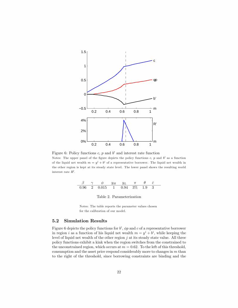
Figure 6: Policy functions c, p and b′ and interest rate functionNotes: The upper panel of the figure depicts the policy functions c, p and b′ as a function
of the liquid net wealth m = yi + bi of a representative borrower. The liquid net wealth in
the other region is kept at its steady state level. The lower panel shows the resulting world
interest rate R′.
β γ φ yH yL π θ c0.96 2 0.015 1 0.94 3% 1.9 3
Table 2. Parameterization
Notes: The table reports the parameter values chosen
for the calibration of our model.
5.2 Simulation Results
Figure 6 depicts the policy functions for b′, φp and c of a representative borrowerin region i as a function of his liquid net wealth m = yi + bi, while keeping thelevel of liquid net wealth of the other region j at its steady state value. All threepolicy functions exhibit a kink when the region switches from the constrained tothe unconstrained region, which occurs atm = 0.62. To the left of this threshold,consumption and the asset price respond considerably more to changes inm thanto the right of the threshold, since borrowing constraints are binding and the
22
economy experiences financial amplification. The policy function b′ is decliningfor constrained values of m since greater liquid net wealth implies a higherasset price and a higher borrowing limit. For unconstrained values of m, thepolicy function b′ is increasing as the agent optimally smoothes consumptionand carries more wealth into the future the more liquid wealth he possesses.The dashed vertical line indicates the level of net wealth that is reached if
the economy has been in the boom state for a long number of periods. Forsimplicity, we call this wealth level the high steady state.The bottom panel of the figure shows the world interest rate R′ as a function
of liquid net wealth m, while keeping the liquid net worth in the other region atits steady state level. The interest rate is a mirror image of the policy functionb′ —the more the agent borrows, the higher the interest rate that internationalinvestors demand.When a region is in its high steady state and experiences a bust shock
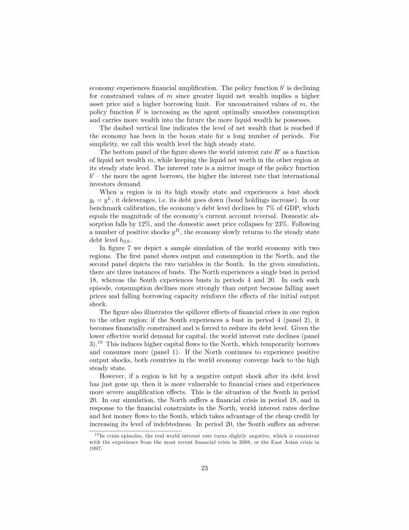
yt = yL, it deleverages, i.e. its debt goes down (bond holdings increase). In ourbenchmark calibration, the economy’s debt level declines by 7% of GDP, whichequals the magnitude of the economy’s current account reversal. Domestic ab-sorption falls by 12%, and the domestic asset price collapses by 23%. Followinga number of positive shocks yH , the economy slowly returns to the steady statedebt level bSS .In figure 7 we depict a sample simulation of the world economy with two
regions. The first panel shows output and consumption in the North, and thesecond panel depicts the two variables in the South. In the given simulation,there are three instances of busts. The North experiences a single bust in period18, whereas the South experiences busts in periods 4 and 20. In each suchepisode, consumption declines more strongly than output because falling assetprices and falling borrowing capacity reinforce the effects of the initial outputshock.The figure also illustrates the spillover effects of financial crises in one region
to the other region: if the South experiences a bust in period 4 (panel 2), itbecomes financially constrained and is forced to reduce its debt level. Given thelower effective world demand for capital, the world interest rate declines (panel3).10 This induces higher capital flows to the North, which temporarily borrowsand consumes more (panel 1). If the North continues to experience positiveoutput shocks, both countries in the world economy converge back to the highsteady state.However, if a region is hit by a negative output shock after its debt level
has just gone up, then it is more vulnerable to financial crises and experiencesmore severe amplification effects. This is the situation of the South in period20. In our simulation, the North suffers a financial crisis in period 18, and inresponse to the financial constraints in the North, world interest rates declineand hot money flows to the South, which takes advantage of the cheap credit byincreasing its level of indebtedness. In period 20, the South suffers an adverse10 In crisis episodes, the real world interest rate turns slightly negative, which is consistent
with the experience from the most recent financial crisis in 2008, or the East Asian crisis in1997.
23

0 10 20 300.85
0.90.95
11.05
yN
cN
0 10 20 300.85
0.90.95
11.05
yS
cS
0 10 20 30−2%
0%
2%
4%R
T
Figure 7: Simulated sample path of world economyNotes: This figure illustrates a simulation of the world economy over 32 periods. Panel 1
shows the time path of output and consumption in the North. Panel 2 depicts the same two
variables in the South. Panel 3 reports the path of the world interest rate.
24

0 5 10−10%
−9%
−8%
−7%
−6%
−∆b
t
0 5 10−15%
−14%
−13%
−12%
−11%
−10%
∆c
t
Figure 8: Impact of output shock on b and cNotes: Panel 1 of the figure shows the impact of adverse output shocks on debt in one region t
periods after the other region has experienced a financial crisis. Panel 2 illustrates the impact
of such shocks on consumption.
shock and experiences a crisis that is significantly larger than the one in period4 —absorption declines by 13.7% instead of 12%.Figure 8 shows the impact of an adverse output shock yL on the level of
debt (panel 1) as well as on consumption (panel 2) t periods after a financialcrisis in the other region. The decline in borrowing −∆b can be interpreted asthe extent of deleveraging in the economy and will materialize in the form of acurrent account reversal. The baseline —an adverse shock without a precedingcrisis in the other region —is depicted for t < 0 and consists of a 7.3% decline inborrowing capacity and a 12% decline in consumption. If the shock hits in theaftermath of crises in other parts of the world economy, the decline in borrowingcapacity is up to 9%, and the decline in consumption up to 14.6%.
5.3 Policy Measures
Given the risk of financial amplification effects and the associated externalities,policymakers in the described economies find it optimal to impose Pigouviantaxes on foreign borrowing in good times so as to mitigate the crises that occurin response to adverse shocks.In our benchmark calibration, a planner finds it optimal to impose a tax on
25

foreign borrowing in the amount of 1.89% in the high steady state. For example,if a borrower took on $100 in foreign credit, the planner would impose a Pigou-vian tax of $1.89 per year. According to equation (15), in an economy with2% inflation, the same effect could be achieved by imposing an unremuneratedreserve requirement in the amount of 35%, i.e. if a borrower took on $100 inforeign credit, he would be required to hold $35 of that amount in an unremu-nerated reserve account. These magnitudes of inflow taxation or unremuneratedreserve requirements are within the range of policy measures that have recentlybeen enacted by a number of emerging economies.11
If a financial crises occurs somewhere else in the world economy, it is desirableto raise the tax to lean against the resulting flows of hot money. The top panelof figure 9 depicts the optimal macroprudential tax t periods after a crisis hasoccurred in the other region of the world economy. In the period the crisisoccurs, the optimal level of the tax is 1.97%, and the corresponding reserverequirement would be 53%. Over the ensuing periods, it falls progressively backto the steady state level.Panels 2 and 3 of the figure replicate the results of figure 8 given the optimal
level of macroprudential taxation. The figures show the impact of an adverseshock in one region t periods after an adverse shock has occurred in the otherregion. The dashed line represents the impact in the decentralized equilibriumand the solid line under a planner’s optimal intervention. The tax on foreignborrowing mitigates the effects of an adverse shock on consumption from 12%to 8.8% in the high steady state of the world economy. When the country hasexperienced inflows of hot money in the aftermath of a crisis in another region,the tax reduces the impact of an adverse shock on consumption from 13.7%to 10%. Similarly, optimal taxation reduces the current account reversal from7.3% to 3.4% in the high steady state of the world economy, and from 9% to4.4% when a country has experienced inflows of hot money in the aftermath ofa financial crisis somewhere else.We simulated the evolution of the world economy and the optimal macro-
prudential tax over a period of 200 time periods and depict the relationshipbetween the optimal tax on the level of debt in a given region in figure 10. Itcan be seen that there is a very close relationship between the two variablesthat is almost linear. Regressing the optimal tax rate on a constant and theeconomy’s level of debt yields that
τ t = −.27− .87bt
with an R2 of .97.Interpreting this relationship as a simple policy rule, an increase in capital
inflows/GDP by 1 percentage point warrants an increase in the optimal level ofcapital inflow taxation by .87 percentage points in our sample economy. If networth rises above b = −.31 in our example, the optimal level of the tax becomeszero as there is no risk of financial crisis in the following period.11For example, Brazil imposed a 2% tax on capital inflows in Oct. 2009, which was later
raised to 6%. Thailand implemented a 30% URR from 2006 to 2008, and Colombia a 40%URR in 2007, which was later increased to 50%. See Ostry et al. (2011).
26

0 5 10
1.6%
1.8%
2%
2.2%
τ
t
0 5 10−10%
−5%
0%
−∆b
t
0 5 10
−10%
−5%
0%
∆c
t
Figure 9: Optimal macroprudential taxation and impact of output shocksNotes: Panel 1 of this figure reports the optimal level of macroprudential taxation in one
region t periods after the other region has experienced a financial crisis. Panels 2 and 3 report
the impact of adverse output shocks on borrowing and consumption: the solid lines represents
the impact given the optimal policy intervention. For comparison, the dashed lines show the
impact in the decentralized equilibrium.
27

0.0%
0.5%
1.0%
1.5%
2.0%
2.5%
3.0%
3.5%
‐0.35 ‐0.34 ‐0.33 ‐0.32 ‐0.31
Wealth level b
Figure 10: Response of macroprudential tax to changes in debtNotes: The figure shows the relationship between the optimal macroprudential tax and the
level of debt in a simulation of the world economy over 200 time periods.
It is also interesting to observe the effects of optimal capital flow taxationon the level of world interest rates. In the decentralized equilibrium withoutintervention, the world interest rate is 3.3% in the high steady state. If oneregion experiences a financial crisis, the resulting current account reversal pushesdown the world real interest rate to —.5%. On the other hand, when all countriesimpose the optimal level of macroprudential regulation, the world real interestrate is 1.6% in steady state, and it declines to only —.2% in the event of a crisis.In welfare terms, we find that optimal capital inflow taxation increases a
country’s welfare in our model by the equivalent of a permanent increase inconsumption by .4%, which is higher than most estimates of the welfare cost ofbusiness cycles.
6 Conclusions
This paper has developed a simple model of hot money and serial financial crises.Money is “hot”in the sense that countries that borrow and later suffer adverseshocks become subject to financial amplification effects that lead to a coordi-nated decline in consumption, borrowing, and asset prices. Individual marketparticipants do not internalize that they expose their country to such amplifica-tion effects when they make their privately optimal borrowing decisions. As aresult, they create an externality on other borrowers. A policymaker can inducemarket participants to internalize these effects by imposing macroprudentialpolicies such as prudential controls on capital inflows. Such measures reducemacroeconomic volatility and improve welfare in the domestic economy.The main focus of the paper was to show that crises in one region of the
world economy lead to higher flows of hot money to other regions, which become
28

in turn more vulnerable to future financial crises. For example, we showed thatan adverse shock of a given size that normally leads to a 12% decline in domesticabsorption will cause a 14.6% decline in domestic absorption if a country hasjust experienced inflows of hot money. By imposing a macroprudential tax oncapital inflows of close to 2%, these magnitudes can be reduced to 8.8% and10% respectively.
The admissibility of capital controls as a tool of macroeconomic managementhas recently been endorsed by researchers at the IMF (see e.g. Ostry et al., 2010,2011), who propose that controls on capital inflows may indeed be desirablefor countries who experience overvalued exchange rates and who have suffi centreserves and adequate fiscal and monetary policy. Our paper highlights oneparticular mechanism that provides a welfare rationale for such controls. We findthat capital controls may also be desirable in case a country experiences assetprice booms that are fuelled by capital inflows, not only in case of appreciationsin the exchange rate, since the reversal of the credit flows that led to booms inasset prices may trigger financial amplification effects in which declining assetprices entail pecuniary externalities.12
The empirical literature, as summarized e.g. by Magud et al. (2011), findsthat capital controls are generally effective in altering the composition of inflows,to some extent effective in reducing exchange rate pressures, but not necessarilyeffective in curbing the total volume of inflows. If the composition of inflowsis successfully altered in favor of contingent financial instruments such as FDIor local currency debt, the externalities discussed in this paper will be reducedand the vulnerability to crisis will be diminished, as shown e.g. in Korinek(2009, 2010). In general, empirically identifying the effects of capital controlson the volume of inflows is diffi cult because of endogeneity problems —controlsare most likely to be imposed when capital inflows are large, but this does notimply that capital controls cause larger inflows.Forbes (2005) argues that capital controls may be undesirable since they
increase the cost of finance. However, increasing the cost of borrowing fromabroad so as to raise the private cost to the social cost is precisely the goal ofsuch controls —the higher prices provide a market signal to borrowers to reducethe activity that imposes negative externalities on the rest of their economy.
There are a number of directions in which our research could be extended.One set of issues that deserves further analysis are the links between financialstability and growth. We analyzed the problem of hot money and serial financialcrises in a model of an endowment economy, but our findings are likely to bevery relevant for production economies. In such economies, private marketparticipants expand the stock of capital during booms and the price of capitalrises, enabling them to take on more credit. During busts, the stock of capitalbecomes less valuable and the collateral value declines. This may lead to afeedback spiral of declining borrowing capacity, falling asset prices, and fire12However, declining exchange rates play a similar role and also entail pecuniary externali-
ties during financial crises. See Korinek (2010).
29

sales. A policymaker who leans against the wind when credit flows into theeconomy may reduce excessive capital creation in booms, which mitigates theneed for fire sales and the decline in asset prices plus the associated credit crunchin case of a bust, thereby increasing social welfare.The problem is even further aggravated if investment has long-term effects
on economic growth. Recent evidence (see e.g. IMF, 2009) suggests that creditcrunches may have long-lasting detrimental effects on output because the in-vestment lost during the crunch cannot be fully made up for during the ensuingrecovery. Under such circumstances the welfare costs of financial crises are sig-nificantly greater than what we found in our numerical results because theystretch over many periods. See Jeanne and Korinek (2011a) for an investigationalong these lines.
7 References
Aoki, Kosuke, Gianluca Benigno and Nobhuiro Kiyotaki (2008), “Capital Flowsand Asset Prices,”in Clarida, Richard H. and Francesco Giavazzi (eds.), NBERInternational Seminar on Macroeconomics 2007, University of Chicago Press.
Bianchi, Javier (2011), “Overborrowing and Systemic Externalities in theBusiness Cycle,”forthcoming, American Economic Review.
Bernanke, Ben S. and Mark Gertler (1989), “Agency Costs, Net Worth, andBusiness Fluctuations,”American Economic Review 79, pp. 14-31.
Caballero, Ricardo J., Emmanuel Farhi and Pierre-Olivier Gourinchas (2008),“Financial Crash, Commodity Prices and Global Imbalances,”Brookings Paperson Economic Activity, Fall 2008, pp. 1-55.
Caballero, Ricardo and Arvind Krishnamurthy (2003), “Excessive DollarDebt: Financial Development and Underinsurance,”Journal of Finance 58(2),pp. 867-894.
Devereux, Michael B. and James Yetman (2010), “Financial Deleveragingand the International Transmission of Shocks,”manuscript, University of BritishColumbia.
Forbes, Kristin J. (2005), “The Microeconomic Evidence on Capital Con-trols: No Free Lunch,”NBER Working Paper 11372.
Frankel, Jeffrey A. and Andrew K. Rose (1996): “Currency Crashes inEmerging Markets: an Empirical Treament,” Journal of International Eco-nomics 41, p. 351-366.
International Monetary Fund (2009), “What’s the Damage? Medium-termOutput Dynamics After Banking Crises,”Chapter 4 in World Economic Out-look, October 2009.
30

Jeanne, Olivier and Anton Korinek (2010), “Managing Credit Booms andBusts: A Pigouvian Taxation Perspective,”NBER Working Paper 16377.
Jeanne, Olivier and Anton Korinek (2011a), “Booms, Busts and Growth,”manuscript, University of Maryland.
Jeanne, Olivier and Anton Korinek (2011b), “Macroprudential RegulationVersus Mopping Up After the Crash,”manuscript, University of Maryland.
Kiyotaki, Nobuhiro and John H. Moore (1997), “Credit Cycles,”Journal ofPolitical Economy 105(2), 211-248.
Korinek, Anton (2007), “Dollar Borrowing in Emerging Markets,”Disserta-tion, Columbia University.
Korinek, Anton (2009), “Excessive Dollar Borrowing in Emerging Markets:Amplification Effects and Macroeconomic Externalities,”manuscript, Univer-sity of Maryland.
Korinek, Anton (2010), “Regulating Capital Flows to Emerging Markets:An Externality View," manuscript, University of Maryland.
Korinek, Anton (2011a), “Foreign Currency Debt, Risk Premia and Macro-economic Volatility,”European Economic Review 55, pp. 371-385.
Korinek, Anton (2011b), “Systemic Risk-Taking: Amplification Effects, Ex-ternalities, and Regulatory Responses,”manuscript, Department of Economics,University of Maryland.
Korinek, Anton, Agustin Roitman and Carlos A. Végh (2010), “Decouplingand Recoupling,”American Economic Review P&P 100(2), pp. 393-397.
Lorenzoni, Guido (2008), “Ineffi cient Credit Booms,”Review of EconomicStudies 75(3), 809-833.
Magud, Nicolas E., Carmen M. Reinhart and Kenneth S. Rogoff (2011),“Capital Controls: Myth and Reality —A Portfolio Balance Approach,”NBERWorking Paper 16805.
Martin, Alberto and Jaume Ventura (2011), “Theoretical Notes on Bubblesand the Current Crisis,”IMF Economic Review 59(1), 6-40.
Mendoza, Enrique G. (2001), “The Benefits of Dollarization when Stabiliza-tion Policy Lacks Credibility and Financial Markets are Imperfect,”Journal ofMoney, Credit and Banking 33.
31

Mendoza, Enrique G. (2010), “Sudden Stops, Financial Crises and Lever-age,”American Economic Review 100(5), pp. 1941-1966.
Nguyen, Ha M. (2010), “Credit Constraints and the North-South Transmis-sion of Crises,”manuscript, World Bank.
Ostry, Jonathan D., Atish R. Ghosh, Karl Habermeier, Marcos Chamon,Mahvash S. Qureshi, and Dennis B.S. Reinhardt (2010), “Capital Inflows: TheRole of Controls,”IMF Staff Position Note 10/04.
Ostry, Jonathan D., Atish R. Ghosh, Karl Habermeier, Luc Laeven, MarcosChamon, Mahvash S. Qureshi, and Annamaria Kokenyne (2011), “ManagingCapital Inflows: What Tools to Use?”Staff Discussion Note 11/06.
Reinhart, Carmen M. and Vincent R. Reinhart (2008), “Capital Flow Bonan-zas: An Encompassing View of the Past and Present,”NBER Working Paperw14321.
Reinhart, Carmen M. and Kenneth S. Rogoff (2009), This Time is Different:Eight Centuries of Financial Folly, Princeton University Press.
Tobin, James (1978), “A Proposal for International Monetary Reform,”Eastern Economic Journal 4(3-4), July/October, pp. 153-159.
32

A Data Sources
The stylized facts reported in the introductory part of the paper are based onfour sets of variables that we obtained at annual frequency for 176 countriesover the period of 1980-2009: As an indicator for the world interest rate, weuse 10-year US Treasury bond yields deflated by the US consumer price index,which is smoothed by taking a three year moving average so as to remove sud-den unexpected changes in inflation. Both variables are taken from the IMF’sInternational Financial Statistics (IFS) database.The dummy variable for capital flow bonanzas is calculated using IFS data
according to the procedure of Reinhart and Reinhart (2008), i.e. a bonanzaoccurs when a country’s current account balance as a percentage of GDP is inits top quintile. Dummy variable for banking crises are obtained from Reinhartand Rogoff (2009), Table A.3.1170. Dummy variables for currency crises arecalculated using IFS data according to the procedure of Frankel and Rose (1996),i.e. a currency crisis occurs if a country’s exchange rate depreciates by morethan 25%, and if this depreciation in turns is at least 10% more than in thepreceding period. Finally dummies for all crises are constucted by combiningbanking and currency crisis dummies.The Granger causality tests in table 1 were performed using fixed effects
panel regressions. We first included lags of the dependent variable and foundthat the only the first lag was significant. Then we augmented the regressionwith lagged values of the independent variable. In table 1 we report the resultingparameters and the associated t-values in parentheses. In both tests that arereported we can reject the hypothesis that the independet variables does notGranger-cause the dependent variable at the .1% level.We also investigated a potential causal link between US banking crises and
US 10-year bond yields by constructing an indicator of US bank failures fromthe FDIC list of failed banks as a proxy for banking sector problems in theUS. However, we could not establish Granger-causality since FDIC assistanceseemed to occur with a significant lag to the actual occurance of banking sectorproblems.
B Numerical Solution Method
Our numerical solution method is an extension of the endogenous gridpointbifurcation method of Jeanne and Korinek (2010). Denote the beginning ofperiod bond holdings for a representative agent in region i as b and for an agentin region j as d. The interest rate is a function of aggregate worldwide borrowingR = R (b+ d) as given by (2). Denote the total beginning of period liquidwealth holdings of agents in the two regions as m = b + y and n = d + z. Ourproblem is to obtain policy functions c (m,n), p (m,n), λ (m,n) and b′ (m,n).By symmetry this latter function is identical to d′ (n,m).Taking advantage of the effi ciency gains provided by the endogenous grid-
point bifurcation method requires setting up the problem in two nested loops.
33

B.1 Outer Loop
At the beginning of iteration k in the outer loop, we start with the policyfunctions ck (m,n), pk (m,n), λk (m,n) and b′k (m,n), which is symmetric tod′k (m,n). (The initial policy functions can be set arbitrarily.)
B.2 Inner Loop
Each inner loop iteration starts with a given set of policy functions cl (m, d′),pl (m, d
′) and λl (m, d′). (The initial functions can be set arbitrarily.) Takingd′k (m,n) from the outer loop as given, we calculate c (m,n) = cl (m, d
′k (m,n))
and similarly for p and λ. In order to take advantage of the endogenous grid-points method, it is useful to perform our iterations over the grid (b′, d′) ofend-of-period wealth levels. For any pair (b′, d′), we calculate the world interestrate R (b′, d′) = R (b′ + d′), which is obtained from lenders’optimality condition(2). Then we define
C (b′, d′) = E[c (m′;n′)
−γ]
P (b′, d′) = E{c (m′;n′)
−γ · [y′ + p (m′;n′)]}
Then we solve the system of optimality conditions first under the assumptionthat the borrowing constraint is loose.
cunc (b′; d′) = {βR (b′ + d′)C (b′, d′)}−1γ ,
punc (b′; d′) =βP (b′, d′)
cunc(b′; d′)−γ,
λunc = 0,
munc (b′, d′) = cunc(b′, d′) +b′
R (b′ + d′).
In the same way, we can solve for the constrained branch of the system forb′ ≤ 0 under the assumption that the borrowing constraint is binding in thecurrent period as
pcon (b′, d′) =−b′/R (b′ + d′)
φ,
ccon (b′, d′) =
[βP (b′, d′)
pcon(b′, d′)
]− 1γ
,
λcon (b′, d′) = ccon (b′, d′)−γ − βR (b′ + d′)C (b′, d′) ,
mcon (b′, d′) = ccon(b′, d′) +b′
R (b′ + d′).
Concatenating constrained and unconstrained results as in Jeanne and Ko-rinek (2010) allows us to obtain policy functions cl+1 (m, d′), pl+1 (m, d′) and
34

λl+1 (m, d′) as well as w′l+1 (m, d′). The steps are iterated until convergence isreached. By employing the endogenous gridpoint bifurcation method, this loopconverges very quickly.
Once the inner loop is completed, we observe that the two functions b′l+1 (m, d′)
and the symmetric d′l+1 (n, b′) can be combined to
b′ = b′l+1
(m, d′l+1 (n, b′)
)Finding the root of this equation yields a function b′k+1 (m,n) and the sym-
metric function d′k+1 (n,m). This step is computationally more costly. How-ever, by alternating iterating on the (effi cient) inner loop with iterating on the(computationally costly) outer loop, the problem can be solved in an effi cientmanner. We substitute d′k+1 (m,n) into cl (m, d′), pl (m, d′) and λl (m, d′) toobtain ck+1 (m,n), pk+1 (m,n), λk+1 (m,n) and iterate until convergence.
35