Household Debt and Business Cycles Worldwide

Atif Mian

Princeton University and NBER

Amir Sufi

University of Chicago Booth School of Business and NBER

Emil Verner

Princeton University

January 2016

Abstract

A rise in the household debt to GDP ratio predicts lower output growth and a higher unemploymentrate over the medium-run, contrary to standard open economy macroeconomic models in which anincrease in debt is driven by news of better future income prospects. GDP forecasts by the IMFand OECD underestimate the importance of a rise in household debt to GDP, giving the change inthe household debt to GDP ratio of a country the ability to predict growth forecasting errors. Thepredictive power of a rise in household debt to GDP ratios is significantly stronger in countries witha fixed exchange rate and countries with a floating exchange rate but against the zero lower boundon nominal interest rates. A rise in household debt to GDP is associated contemporaneously witha rising consumption share of output, a worsening of the current account balance, and a rise inthe share of consumption goods within imports. Taken together, these results are consistent withdemand externality models where credit supply shocks result in households borrowing more than issocially optimal given the presence of nominal rigidities and monetary policy constraints.. We alsodocument a global household debt cycle with an increase in household debt to GDP at the globallevel predicting lower global output growth.

∗This research was supported by funding from the Initiative on Global Markets at Chicago Booth, the Fama-

Miller Center at Chicago Booth, and Princeton University. We thank Giovanni Dell’Ariccia, Andy Haldane, Oscar

Jorda, Anil Kashyap, Guido Lorenzoni, Virgiliu Midrigan, Emi Nakamura, Jonathan Parker, Chris Sims, Alan

Taylor, and seminar participants at Princeton University, Northwestern University, the Swedish Riksbank confer-

ence on macro-prudential regulation, Danmarks Nationalbank, the NBER Monetary Economics meeting, and the

NBER Lessons from the Crisis for Macroeconomics meeting for helpful comments. Elessar Chen and Seongjin

Park provided excellent research assistance. Mian: (609) 258 6718, atif@princeton.edu; Sufi: (773) 702 6148,

amir.sufi@chicagobooth.edu; Verner: verner@princeton.edu. Link to the online appendix.

The Great Recession has sparked new questions about the relation between household debt and

the macroeconomy. Recent theoretical and empirical reseach recognizes that a sudden and large

increase in household debt can lower subsequent output growth in the presence of monetary and

fiscal policy constraints. Moreover, households may not internalize the effect of their individual

borrowing decision, making the economy at times susceptible to “excessive” credit growth.1

However, empirical evidence on increases in household debt and subsequent economic perfor-

mance is largely limited to the United States and the most recent global recession. A more system-

atic evaluation of the empirical relation between household debt and business cycles worldwide is

needed in order to understand if recent events have broader implications. This is especially impor-

tant given the dramatic rise in household credit to GDP ratios over the last 50 years documented

by Jorda et al. (2014a).

In this study, we compile data for 30 (mostly advanced) countries from 1960 to 2012 and

document several new results that have important implications for modeling the relation between

changes in household debt and business cycles. We begin by showing that an increase in the

household debt to GDP ratio over a three year period in a given country predicts subsequently

lower output growth.2 The magnitude of the predictive relation is large – a one standard deviation

increase in the household debt to GDP ratio over the last 3 years (6.2 percentage points) is associated

with a 2.1 percentage point decline in GDP over the next three years. This relation is robust across

time and space. Moreover, an increase in the household debt to GDP ratio predicts an increase in

the future unemployment rate, suggesting that the decline in output growth reflects an increase in

economic slack.

What economic model best explains the negative relation between household debt changes and

subsequent output growth? One potential explanation is that the relation is driven by underly-

ing productivity or permanent income shocks in a standard open economy, representative-agent

macroeconomic model. However, the most basic version of such a model is inconsistent with the

facts. As we show, in the most basic version of this type of model, a change in household debt

1See, e.g., Mian and Sufi (2014) and IMF (2012) for empirical evidence and Eggertsson and Krugman (2012), Guerrieriand Lorenzoni (2015), Farhi and Werning (2015), Korinek and Simsek (2014), Schmitt-Grohe and Uribe (forthcom-ing) and Martin and Philippon (2014) for theoretical analysis.

2We follow standard time-series econometrics semantics and use the term “predict” to refer to the predicted value ofan outcome using the entire sample used to estimate the regression. This is in contrast to the term “forecast” thatrefers to the estimated value of the outcome variable for an observation that is not in the sample used to estimatethe regression coefficients. See Stock and Watson (2011), chapter 14.

1

is driven by a corresponding change in expected future income, which yields a positive relation

between increases in household debt and subsequent output growth. We find a negative relation.

Could a more nuanced version of a productivity or permanent income-based macroeconomic

model explain our results? Perhaps, but it would have to be consistent with the following facts

that we show. First, over the medium-run horizon we examine, an increase in the household debt

to GDP ratio robustly predicts a decline in subsequent GDP, whereas an increase in the non-

financial firm debt to GDP ratio has little predictive power after controlling for a rise in household

debt. Second, a rise in household debt is not associated with increased investment growth as

would be predicted by a productivity shock-based model. Instead, when household debt rises, the

consumption share of output increases, as well as the share of imports that are consumption goods.

Further, while an increase in the household debt to GDP ratio predicts lower subsequent output

growth, we show that the slowdown is not anticipated by professional forecasters at the IMF and

OECD. Forecasters continue to ignore the predictive information in increases in household debt,

despite household debt predicting slower output growth in the pre-1990 sample. As a result, an

increase in the household debt to GDP ratio predicts negative forecasting errors by the IMF and

OECD. It is important to note that the forecasts by the IMF and OECD contain useful forecasting

power, but they miss the household debt effect shown here.

It is difficult to reconcile the predictive power of household debt changes on forecasting errors

with an alternative explanation for our results based on news or productivity shocks seen by fore-

casters but not by us. Professional forecasters should adjust their forecasts to take into account

mean reversion or any other information about productivity shocks associated with an increase in

household debt.3 More generally, this result suggests professional forecasters do not appreciate the

predictive power of household debt changes on subsequent output growth.

So what alternative class of models best explains the robust negative relation between household

debt changes and subsequent output growth? Recent theoretical work, highlighted above, suggests

that an expansion in credit supply may lead households to borrow and consume more than is socially

desirable. Households borrow excessively because of aggregate demand externalities associated with

nominal rigidities and constraints on monetary policy. In theory, the combination of credit supply

3Of course, it could be that professional forecasters systematically miss some news shocks or mean reversion inproductivity shocks, but that would call into question the assumption of rational expectations over future innovationsto productivity.

2

shocks, excessive household borrowing, and aggregate demand externalities results in a negative

relation between changes in household debt and subsequent output growth.

We find a number of results that are broadly supportive of this alternative class of models.

First, household debt growth is indeed correlated with consumption booms. We find that a rise in

the household debt to GDP ratio is contemporaneously correlated with a rise in the consumption

share of output and a decline in the net export to output ratio. As mentioned above, the decline

in net exports is driven by an increase in the share of imports that are consumption goods.

Second, monetary policy frictions are closely related to the severity of the slowdown in the

aftermath of a credit boom. We explore heterogeneity in the predictive relation between changes in

household debt and subsequent output growth, and we show that the negative relation is strongest

in fixed exchange rate regimes versus more flexible exchange rate regimes. Similarly, the relation is

stronger during zero lower bound episodes within flexible exchange rate regimes, and stronger when

the increase in household debt is financed externally. These results suggest that nominal rigidities

and monetary policy constraints matter.

Third, we attempt to isolate the rise in the household debt to GDP ratio driven by credit supply

shocks. We argue that time-series variation in the sovereign yield spread of a country relative to

U.S. Treasuries can be useful in testing the impact of an expansion in credit supply on private

debt growth and subsequent output growth. Prior research shows that variation in sovereign yield

spreads can be driven by non-country specific fundamentals such as changes in the risk premium

required by financiers (Remolona et al. (2007), Longstaff et al. (2011), and Bofondi et al. (2013)).

Further, to the extent that country fundamentals are driving variation in the sovereign yield spread,

it would lead to the opposite prediction to what we find in the data. In particular, a fall in the

sovereign yield spread should be reflective of better economic fundamentals going forward.

We use the lagged sovereign yield spread as an instrument for changes in household debt to

GDP, and we show that a fall in the sovereign spread leads to an increase in the country’s household

debt to GDP ratio. The second-stage shows that the sovereign spread-induced increase in household

debt predicts lower subsequent GDP growth. An example is the experience of peripheral European

countries when they joined the Eurozone. They experienced a drop in sovereign yields and a

dramatic rise in household debt, which was followed by a severe decline in output. The same result

holds for the United States when we use the high yield share of firm debt issuances as a proxy for

3

an increase in credit supply, as suggested by Greenwood and Hanson (2013). Taken together, the

facts are more consistent with models in which credit supply varies over time and nominal rigidities

matter; they are less consistent with models where fluctuations are driven by productivity shocks.

In the last section of the study, we explore the global implications of the relation between changes

in household debt and output growth at the country level. We show that when an economy slows

down in the aftermath of a rise in household debt, net exports increase due to a contraction in

imports. There are therefore spillover effects from one country to another, suggesting that the

global economy relation between household debt changes and subsequent output growth may be

even stronger than what we estimate at the country level. Moreover, if many countries experience

a post-debt hangover at the same time, the net export margin will be less able to stabilize the

economy of any given country.

We find support for both of these hypotheses. First, countries with a household debt to GDP

cycle that is more strongly correlated with the global debt cycle see a stronger decline in future

output growth after a rise in the household debt to GDP ratio. Second, there is a much stronger

negative relation between the rise in global household debt to GDP and subsequent global growth.

As before, this negative relation is only associated with the household debt to GDP ratio. A rise

in the global non-financial firm debt to GDP ratio has no predictive power for global GDP growth

over the medium term horizon.

The relation between a rise in global household debt and subsequent slowdown in GDP growth

is not driven by the post-2000 period alone. In fact, using estimates from only pre-2000 data, we

show that our regression model forecasts (out-of-sample) quite accurately the slowdown in global

growth during the late 2000s given the dramatic rise in global household debt during the mid-2000s.

Our paper follows the recent influential work by Jorda et al. (2014a), Schularick and Taylor

(2012), Jorda et al. (2013), and Jorda et al. (2014b) on the role of private debt in the macroe-

conomy. The authors put together long-run historical data for advanced economies to show that

credit growth, especially mortgage credit growth, predicts financial crises (also see Dell’Ariccia

et al. (2012)). Moreover, conditional on having a recession, stronger credit growth predicts deeper

recessions.4

4There is also cross-sectional evidence from the recent recession in the United States and Europe (see, e.g., Mianand Sufi (2014), Glick and Lansing (2010), and IMF (2012)) showing that areas with the largest rise in householddebt during the boom saw the biggest decline in economic activity during the bust. Baron and Xiong (2014) show

4

Our methodological point of departure from the above literature is that we focus on estimating

the unconditional relation between changes in household debt and subsequent GDP growth, while

earlier work focuses on the effect of increases in credit on recession severity conditional on having

a recession. Further, our analysis provides a number of new results that should guide the nascent

theoretical literature on private credit and business cycles. For example, our results on the asym-

metry between household debt and non-financial firm debt, predictability of labor market slackness,

as well as predictability of GDP forecast errors help rule out spurious factors that could produce a

relation between changes in household debt and subsequent GDP growth. Our findings regarding

the consumption boom, heterogeneity with respect to monetary regimes, and the influence of credit

shocks on household debt changes are important for understanding the mechanisms that generate

the negative relation between household debt changes and subsequent GDP growth. Finally, our

results on the external margin spillovers highlight the importance of the “global household credit

cycle,” which was also an important precursor to the most recent global recession.

While the existing literature in macro-finance has made important contributions in understand-

ing the “investment” channel for business cycle dynamics (see e.g., Bernanke and Gertler (1989),

Kiyotaki and Moore (1997), Caballero and Krishnamurthy (2003), Brunnermeier and Sannikov

(2014) and Lorenzoni (2008)), our results highlight the importance of a debt-driven “consumption”

channel for business cycle dynamics. We hope our results will help guide the burgeoning theoret-

ical literature in this area, such as Eggertsson and Krugman (2012), Farhi and Werning (2015),

Guerrieri and Lorenzoni (2015), Korinek and Simsek (2014), Martin and Philippon (2014), and

Schmitt-Grohe and Uribe (forthcoming).5

The remainder of the paper is structured as follows. The next section presents the data and sum-

mary statistics. Section 2 presents the empirical specification. Sections 3 and 4 provide empirical

estimates of the relation between household debt changes, output growth, changes in unemploy-

that a large increase in bank credit to GDP predicts lower equity returns, and Cecchetti and Kharroubi (2015)find that the growth in the financial sector is correlated with lower productivity growth. Cecchetti et al. (2011)estimate country-level panel regressions relating economic growth from t to t + 5 to the level of government, firm,and household debt in year t. They do not find strong evidence that the level of private debt predicts growth.Reinhart and Rogoff (2009) provides an excellent overview of the patterns of financial crises throughout history.

5While we have restricted our attention here to models where over-borrowing is driven by an externality, we donot argue that behavioral biases are unimportant. For example, households may overborrow due to hyperbolicpreferences as in Laibson (1997) or a“neglected risk” as in Gennaioli et al. (2012). Such excessive borrowing canthen lead to a slowdown in output growth, as in Barro (1999). Further, we do not take a stand on what drives thevariation in credit supply, which could be driven by behavioral biases such as sentiment shifts. We do, however,believe that debt is an important part of the story. We discuss this point further in the conclusion.

5

ment, and GDP forecasts. Section 5 presents evidence on the consumption boom, heterogeneity

with respect to monetary policy frictions, and credit shocks. Section 6 presents evidence on the

global household debt cycle, and section 7 concludes.

1 Data and Summary Statistics

1.1 Data

We build a country-level unbalanced panel dataset that includes information on household and

non-financial firm debt to GDP, national accounts, unemployment, professional GDP forecasts,

and international trade. The countries in the sample and the years covered are summarized in

Table 1. The data are annual and range from 1960 to 2012, providing over 900 country-years

before taking differences. Details on variable definitions and data sources are provided in the online

data appendix. Here we briefly describe the key variables measuring expansions in household and

non-financial firm debt.

We measure household and non-financial firm debt expansions as the change in the household

debt to GDP ratio and the change in the non-financial firm debt to GDP ratio, respectively. We

justify this decision in the next section. We denote the change in household and firm debt to

GDP ratio from year t − k to year t by ∆k(HHD/Y )t and ∆k(FD/Y )t, where HHD and FD

are the outstanding levels of credit to households and non-financial corporations, respectively,

at the end of year t. Credit is defined as loans and debt securities financed by domestic and

foreign banks, as well as non-bank financial institutions. Outstanding credit to households and

non-financial corporations are from the BIS’s “Long series on credit to the private non-financial

sector” database. This database has quarterly information on total credit to the private non-

financial sector and decomposes total credit into credit to households and credit to non-financial

firms.6

6The series on credit to households and non-financial firms are available for 34 countries. We exclude China, India,and South Africa, as the decomposed credit series are only available from 2006 for China and South Africa and 2007for India. We also exclude Luxembourg, as the data on non-financial firm credit for Luxembourg is highly volatile,with changes of similar magnitude as annual GDP in some years.

6

1.2 Summary Statistics

Table 2 displays summary statistics for the change in total private, household, and non-financial

firm debt to GDP, as well as the other variables.7 Our empirical analysis uses both annual changes

in panel Vector Autoregressions (VARs) and changes over three years in a single equation estimation

framework. Table 2 shows that total private sector debt to GDP, PD/Y , has been increasing by

3.11 percentage points per year on average, with household debt to GDP increasing slightly more

quickly than non-financial firm debt. The change in non-financial firm debt is about two times as

volatile as household debt, and both series are reasonably persistent. Other patterns documented

in Table 2 are consistent with the small open economy business cycle literature. Total consumption

expenditure is approximately as volatile as output, while durable consumption and investment are

about 2.8 and 3.6 times as volatile as output, respectively. Imports and exports are roughly four

times more volatile than output.

2 Conceptual Framework and Empirical Specification

We adopt the local projections method introduced by Jorda (2005) to analyze the predictive rela-

tionship between changes in debt and subsequent macroeconomic variables. The general specifica-

tion we utilize is as follows. For a given country, let yt be the natural logarithm of GDP in year t,

and ∆yt+h = yt+h−yt. Let dHHt be a measure of household debt in year t and ∆kdHHt = dHHt −dHHt−k

be the change in household debt from t−k to t. Then, in its most simple form, the impulse response

function (IRF) of output to a change in household debt, ∆kdHHt , can be written as:

∆yt+h = αh + βhHH∆kdHHt + εt, (1)

where βhHH traces out the IRF for a change in household debt from t− k to t for increasing values

of h.

The IRF estimated in equation (1) does not necessarily represent a causal response of output

7With the exception of the serial correlation, all statistics are computed by pooling observations from all countries.The serial correlation is a weighted average of the serial correlations for each country, with the underlying numberof observations for each country as weights.

7

to a change in debt. In order to interpret the IRF properly, we need to put more structure on the

economic relationship between debt and the macroeconomy. In the following two sub-sections, we

describe two classes of models which have the opposite implications for the expected sign of βhHH

from the IRF estimation in equation 1. The standard open-economy representative agent model in

which fluctuations are driven by permanent income shocks implies a positive βhHH , whereas models

with credit supply shocks and aggregate demand externalities predict a negative βhHH .

2.1 Household Debt and Ouput Growth in Standard Open Economy Models

Consider a small open economy with a continuum of infinitely lived households with utility function,

E0

∞∑t=0

βtu(ct).

Households face no borrowing constraints, and there is a risk-free one period bond that can be

traded internationally. Output yt is given exogenously by a stochastic process, and each household

faces a sequential budget tradeoff of the form,

ct + (1 + r)dt−1 = yt + dt. (2)

Optimal allocation of consumption across periods requires that a no-Ponzi game constraint hold

with strict equality,

limj→∞

Etdt+j

(1 + r)j= 0. (3)

Maximizing utility subject to the stochastic income process and the inter-temporal budget con-

straint gives us the traditional Euler equation,

u′(ct) = β(1 + r)Etu′(ct+1).

We assume β(1 + r) = 1, which gives us constant consumption in steady state and simplifies the

exposition. Furthermore, we assume quadratic utility with U(c) = −12(c − c)2 with c ≤ c, which

makes marginal utility linear and hence consumption a random walk with ct = Etct+1. Iterating

8

forward (2) and using (3) and ct = Etct+1, we get that consumption equals expected permanent

income Etypt minus interest payments on outstanding debt rdt−1 in equilibrium,

ct = Etypt − rdt−1 =

r

(1 + r)Et

∞∑j=0

yt+j(1 + r)j

− rdt−1. (4)

Plugging ct = Etypt − rdt−1 into equation (2) we can see that debt evolves according to, dt−dt−1 =

Etypt − yt. Let ∆dt = dt − dt−1 and ψt+jt = Et∆yt+j represent the expected change in income

j periods forward. We can equivalently write down the change in debt at time t in terms of the

present value of expected changes in future income:

∆dt =

∞∑j=1

ψt+jt

(1 + r)j(5)

Equation (5) summarizes the key intuition coming from the standard open economy model.

Growth in household debt is driven by expected future income growth. Expectation of higher

income growth at time t results in consumers increasing their net borrowing in an effort to smooth

consumption over time.

Hypothesis 1: If demand for debt is driven by future income shocks, as in standard open

economy models, the relation between household debt and subsequent growth will be positive. The

coefficient on the increase in household debt, βhHH , in equation (1) will therefore be positive.

In this setting, the estimate of βhHH represents the equilibrium relation between debt and growth,

and should not be interpreted in any causal sense. While the prediction above is derived under

the assumptions of a representative agent, quadratic utility, and an exogenous income process, the

positive predictive relationship between lagged debt growth and output growth is robust to more

generic utility functions and the introduction of capital and endogenous output.8

In estimating βhHH we focus on the qualitative prediction that household borrowing is due to

anticipation of higher future income growth, and we do not attempt to statistically test the restric-

tions implied by the specific quadratic utility model applied to household debt. Prior research has

showed that the present-value quadratic utility model is statistically rejected in the data when ap-

plied to saving and the current account (Campbell (1987) and Nason and Rogers (2006)). Cochrane

8See Uribe and Schmitt-Grohe (2015) for an excellent exposition of the broader open economy macro literature.

9

(1994), however, argues that the qualitative predictions of the permanent income model are valid

for consumption and income for the United States time series, and we therefore ask whether the

same holds for household debt.

Finally, strictly speaking, the debt in this small open economy model represents net foreign

debt. This is due to the assumption of a representative agent. More broadly, one could introduce

heterogeneity where some agents within a country receive a positive productivity shock and borrow

from other agents in the same economy. Our empirical section uses total gross private debt, whether

borrowed domestically or from abroad. But we also show results for net foreign debt.

2.2 Household Debt and Output Growth with Aggregate Demand Externalities

Debt plays a passive role in the standard open economy model highlighted above. It reflects agents’

expectations of future income growth, implying that higher debt growth should be a harbinger of

better economic times. The fact that some famous credit booms have ended badly for the economy

– at least in hindsight – has led to a recent growing literature in macro-finance showing that

in the presence of nominal rigidities and constraints on monetary policy, an economy can have

“excessive” household debt growth that translates into lower output growth going forward. We

derive the empirical implications of these “aggregate demand externality” theories through the

following highly stylized example.9

Consider the same representative agent set up as above, except that there are only two periods,

t and t+ 1. The output capacity of the economy is fixed at y, with yt = y. The first key ingredient

of our stylized model is the presence of nominal rigidities and monetary policy frictions that make

output at t + 1 potentially contingent on the total amount of debt that households borrowed in

period t, Dt, and macroeconomic frictions, Φ. In particular,

yt+1 =

y if Dt ≤ D

y − f(DtD,Φ) with f(1, .) = 0, f1 > 0 and f12 > 0, otherwise

(6)

Equation (6) implies that if households choose to take on “excessive” debt (Dt > D) in period t,

9There are additional models based on pecuniary or fire sales externalities that focus on the potential for excessiveleverage among non-financial firms. Examples include Shleifer and Vishny (1992), Kiyotaki and Moore (1997),Lorenzoni (2008), and Davila (2015). Pecuniary externalities can also amplify the effect of household debt, especiallyfor collateralized borrowing such as mortgages.

10

then the economy cannot operate at full capacity in period t+1. The output shortfall will be larger

with higher levels of household debt and more severe macroeconomic frictions Φ.

We take the relation in equation (6) as given in order to derive empirical implications. But

this relation is formally derived in the models by Eggertsson and Krugman (2012) and Korinek

and Simsek (2014). In both of these models, the authors assume a closed economy with impatient

consumers facing a borrowing constraint. If debt levels are sufficiently high and there exists a

friction on monetary policy such as a zero lower bound, a sudden tightening of the borrowing

constraint pushes the economy into a recession.

Schmitt-Grohe and Uribe (forthcoming) also derive a relation similar to equation (6) in a

representative-agent open-economy model. In their model, a temporary fall in the interest rate, rt,

motivates consumers to borrow at time t and expand their consumption of tradable goods. Since

the maximum output is fixed at y, the shock translates into higher wages. When the interest rate

shock reverses at t + 1, the economy is forced to adjust. However, wage rigidity on the downside

prevents the economy from adjusting fully, resulting in unemployment and decline in output. Notice

that the fall in output at t+1 is driven by a fully anticipated tightening of the borrowing constraint

in Korinek and Simsek (2014), and an upward reversal in interest rates in Schmitt-Grohe and Uribe

(forthcoming). The output dynamics summarized in (6) assume such a shock, which we refer to as

a credit supply shock.10

With next period output defined by equation (6), we can now close the model and solve for the

level of debt chosen by consumers in period t. For simplicity, assume that the economy enters t

with no debt at all, and that there are a continuum of identical households of measure one. Each

household chooses consumption ct, ct+1, and debt dt to maximize utility u(ct) + βu(ct+1), subject

to budget constraints yt = ct − dt1+rt

and yt+1(Dt) = ct+1 + dt.

Since there is measure one of total households, dt = Dt in equilibrium. However, each household

will choose dt, taking as given their equilibrium expectation of Dt. This observation gives rise to

an important “demand” externality in the model: households do not internalize the fact that their

10There are other papers in the macro-finance literature that share some of the features detailed here, includingJustiniano et al. (2015), Favilukis et al. (2015)), Martin and Philippon (2014), and Guerrieri and Lorenzoni (2015).While we have restricted our attention here to models where over-borrowing is driven by an aggregate demandexternality, households may overborrow for behavioral reasons as in models with hyperbolic preferences (Laibson(1997)) or “neglected risks” (Gennaioli et al. (2012)). Such excessive borrowing can then lead to slowdown inoutput growth, as in Barro (1999).

11

choice of debt could lead to lower output next period, leading to excessive borrowing relative to

the social optimum.

The demand externality becomes transparent by comparing the private Euler equation of each

household, in which a household takes Dt as given, with the social planner’s Euler equation who

internalizes the effect of her choice of dt on Dt. The private Euler equation is u′(ct)u′(ct+1) = β(1 + rt),

while the social Euler equation is u′(ct)u′(ct+1) = β(1+rt)(1+f1D

−1). Thus private consumption ct (and

hence borrowing dt) is too high in the decentralized equilibrium relative to the social optimum.

We can now consider the response of a household in period t to a credit shock, which following

Schmitt-Grohe and Uribe (forthcoming) we model as a fall in rt. Assuming log utility, households

take on debt dt = 11+β (yt+1(Dt) − β(1 + rt)y).11 This leads us to the following hypothesis:

Hypothesis 2: In a model with aggregate demand externalities, we derive the following empir-

ical implications: (i) A strong enough positive credit supply shock can lead to excessive growth in

debt, and a decline in subsequent output when the credit supply shock reverses. The coefficient on

lagged increases in debt, βhHH , in equation (1) will be negative, and the relation is non-linear. (ii)

Growth in household debt generates a contemporaneous “consumption boom” and an increase in

net imports, followed by a reversal. (iii) The negative relation between changes in household debt

and subsequent output growth is stronger when macroeconomic frictions such as nominal rigidities

(Φ) are more restrictive.

To reiterate, we develop Hypothesis 2 to give us qualitative implications for the empirical

analysis below. These implications follow from the aggregate demand externality models discussed

above.

2.3 Full Empirical Specification

We augment equation (1) to allow for multiple countries in our sample and a richer set of variables

as is typical in the local projection method. Let yit be the dependent variable of interest, such as

log GDP, for country i in year t. We estimate the IRF for an innovation in debt using:

∆hyi,t+h = αhi + βhHH∆3dHHi,t−1 + βhF∆3d

Fi,t−1 +X ′i,t−1Γh + εit, (7)

11With log utility, we assume D < y(1−β)1+β

, which guarantees that there exists a large enough fall in rt that generatesan output slump in period t+ 1.

12

where αi are country fixed effects, ∆3 refers to the difference over 3 years, i.e., ∆3dHHit = (dHHit −

dHHit−3), dHHit and dFit correspond to the household debt to GDP ratio and the non-financial firm

debt to GDP ratio, respectively, and h = 1, 2, ... is the forecast horizon. The matrix X ′it includes

additional control variables such as higher order lagged polynominals for the dependent variable in

the spirit of the local projections method. As we explain below, we choose to difference the right

hand side debt to GDP ratios over 3 years based on information from auto-regressive specifications.

We lag the right hand side variables by one year to leave some gap before we start estimating the

IRF. Table A1 in the online appendix shows robustness to this particular choice. The coefficients

βhHH and βhF trace out the IRF of y for a change in household debt and a change in non-financial

firm debt, respectively, for increasing values of h.

The debt variables dHHit and dFit refer to debt normalized by the size of the economy. In models

such as Eggertsson and Krugman (2012), it is the size of the change in gross debt relative to the size

of the overall economy that determines whether the economy can fall into a liquidity trap at some

point. For example, if we do not scale debt by GDP, episodes of large real debt growth from a small

base can appear large without being economically meaningful. We use two different normalization

methods. The first method normalizes debt by GDP, with dHHit = HHDitYit

and dFit = FDitYit

, where

HHD and FD refer to nominal household debt and non-financial firm debt respectively, and Y

refers to nominal GDP. A potential drawback of this normalization is that the change in debt to

GDP variable also captures innovations to GDP, and not just debt. We therefore also adopt a second

normalization method, where the change in debt is computed relative to a fixed base year GDP,

i.e., ∆3dHHit = HHDit−HHDit−3

Yit−3. Our empirical results are similar regardless of the normalization

methodology used.

We choose to follow the local projections (LP) method as our default specification due to certain

advantages it offers. First, the LP method is flexible in that it does not constrain the shape of the

IRF between horizons h and h + 1 (unlike a structural vector auto regression, or SVAR). Second,

it does not necessarily require that all variables enter all equations simultaneously and therefore

can provide a more parsimonius specification. Third, the LP approach is flexible and allows for the

estimation of state-dependent βhHH . For example, we can easily test if the coefficient is stronger

in fixed exchange rate regimes where monetary frictions are more likely to bind, or when debt is

borrowed externally (see Ramey and Zubairy (2014) as another example). While we use LP as our

13

default specification, we show robustness of our main results in a more traditional structural SVAR

as well.

Why do we choose a 3-year period when differencing the debt variable? We let the data

tell us the appropriate window over which debt should be differenced. Specifically, for each of

the two components of private debt, household debt and non-financial firm debt, we estimate an

autoregressive(AR) model:

∆HHDit

Yit= µHH +

5∑j=1

ϕHHj ∆HHDit−jYit−j

+ εHHit

∆FDit

Yit= µF +

5∑j=1

ϕFj ∆FDit−1

Yit−j+ εFit .

The AR models include five lags and are estimated on the pooled sample.12

Figure 1 plots the cumulative impulse responses for household and firm debt to GDP from these

autoregressive models. The figure shows that an initial unit impulse to ∆HHDY is amplified for three

to four years before dying out. The cumulative effect is about 2.3 units by the fourth year after

the increase. A shock to ∆FDY also leads to a persistent increase, although the effect of the shock

on firm debt expansion fades more quickly. The cumulative effect on firm debt to GDP is about

1.6 percentage points after 4 years.

The flexible AR therefore points to a three to four year period over which a shock to household

debt persists. This is consistent with studies that have examined particular episodes such as the

growth in household debt in the United States, where Mian and Sufi (2010) use years from 2002

to 2006, or the growth in household debt in Europe, where King (1994) uses years from 1984 to

1988. In the analysis that follows, we set k = 3, and present robustness in Table A1 in the online

appendix to alternative window lengths.

One advantage of our study relative to most of the existing research is that it tests the predictive

power of both household debt and non-financial firm debt on growth in the same specification. In

particular, some economic models feature fundamental shocks that should in principle lead to a

similar correlation of subsequent GDP growth with both household debt and firm debt. Examining

12We choose a lag length of five to be consistent with our VAR results presented below, which use five lags chosenby the Akaike Information Criterion. Schularick and Taylor (2012) also use five lags of credit growth, noting thatcredit booms are typically persistent events.

14

whether there are different correlations of household debt changes and non-financial firm debt

changes with subsequent growth can help us explore which models are most accurate.

In all specifications, standard errors are clustered at the country level to allow for arbitrary

correlation between errors within countries. In particular, this accounts for residual autocorrelation

induced by the overlapping observations. In a robustness check, we use only every third year to

construct a sample of non-overlapping observations, and we show the results are similar. In our

initial set of results, we do not include year fixed effects. We believe that the global time series of

household debt is of independent importance. Consequently, we explore year fixed effects and the

global credit cycle in more detail in Section 6.

Finally, we generally include lagged output growth along with country fixed effects in our main

specification (7). Including lagged output growth controls for any persistence in output growth

that may be correlated with changes in debt to GDP, and country fixed effects capture any omitted

time-invariant factors that affect a country’s growth rate. It is well known, however, that the

fixed effects estimator is biased in the presence of a lagged dependent variable and that this bias

decreases as the time dimension increases to infinity. Although we do not believe that this Nickell

bias is a serious concern in our long panel (the average sample length is 23 years), we report similar

results for the sample of non-overlapping observations using the Arellano and Bond (1991) GMM

estimator that addresses this bias.

3 Household Debt Expansions and Output Growth

3.1 Basic Result, Non-linearities, and Robustness

Table 3 presents estimates of equation (7) with output growth measured at a 3 year horizon, i.e.

h = 3. Column 1 sums household debt and non-financial firm debt and uses the overall change in

private debt to GDP on the right hand side. Columns 2 though 4 separate out the two components

of total private debt. There is a significant negative correlation between changes in private debt

and future output growth. Moreover, this negative correlation is entirely driven by the growth in

household debt (column 4). The magnitude of the negative correlation is large, with a one standard

deviation increase in the change in household debt to GDP ratio (6.2 percentage points) associated

with a 2.1 percentage point lower output three years out.

15

Figure 2 plots the coefficients from equation (7) to trace out the entire impulse response func-

tion. The negative relation between changes in private debt and subsequent output growth comes

exclusively from the rise in household debt. Moreover, the magnitude of the relation increases over

time. Expansions in household debt are associated with a protracted period of low output growth.

Column 5 of Table 3 includes lagged one-year GDP growth variables over the same period as

the change in debt, ∆yi,t−1, ∆yi,t−2 and ∆yi,t−3. The estimate of βhHH is robust to the inclusion

of lagged GDP growth controls, which shows that this result is not driven by some spurious mean

reversion in the output growth process.

Column 6 adds the change in government debt to GDP over the same period on the right hand

side. A rise in government debt to GDP is associated with moderately stronger growth over the

following three years, but the coefficient is small and not statistically significant.13 The negative

relation between future output growth over the medium run and past changes in debt to GDP

ratios is unique to household debt.

So far we have employed a linear regression to estimate the relation between changes in house-

hold debt and future output. As we discussed in the previous section, theories predicting a negative

relation between these variables suggest the relation should be non-linear. We investigate any po-

tential non-linearity by looking at the non-parametric relation between a change in household debt

to GDP ratio and subsequent GDP growth in Figure 3.

Panel a shows that the non-parametric relation between an increase in household debt to GDP

and subsequent growth is non-linear, with larger increases in household debt predicting increasingly

lower growth.14 Ireland and Greece during the Great Recession show up in the bottom right part

of the scatter plot, but several other episodes including Finland from 1989 to 1990 and Thailand

during the East Asian financial crisis also help explain the robust correlation. In particular, while

the overall relationship is negative and non-linear, it is not driven by outliers: the relation is

negative even toward the middle of the distribution. Panels b and c show the partial correlation

between future output growth and the change in household debt to GDP and non-financial firm

debt to GDP ratios, respectively. As already shown in column 4 of Table 3, the partial correlation

is negative for household debt, but flat for non-financial firm debt.

13In Figure A1 in the online appendix we show that this result holds at all horizons between one and five years.14Alternatively, including a quadratic term for the increase in household debt to GDP yields a negative estimate that

is significant at the 6% level in a fixed effects regression.

16

Is the negative overall estimate of β3HH representative of a broad set of countries, or only driven

by a select few? Figure 4 answers this question by providing country-by-country estimates of the

coefficient from estimating equation (7) separately for each country at the three year horizon and

with lagged output growth variables as controls. The coefficient on the household debt to GDP

ratio is negative for twenty-four of the thirty countries in our sample, and none of the country

coefficients are significantly positive with the exception of Turkey.15 The cross-country average of

the estimates is -0.36 and the precision weighted average is -0.40. The average estimates are similar

to the panel data regression estimate in Table 3, which suggests that potential bias arising from

heterogeneous coefficients is not likely to be an important concern.16

Table 4 provides some additional robustness checks on sample selection, standard errors, and

functional form of our debt variables. Columns 1 and 2 show that the βhHH estimate is larger in

absolute value for developed economies (-0.37), but the relation is also strong for emerging market

economies (-0.24). Columns 3 and 4 exclude the post-1990 period and the post-2000 period, showing

that the boom and bust cycle of the Great Recession of 2008 is not uniquely responsible for our

results. Column 5 focuses only on the last 30 years, and finds a similar result. While we adjust

all our standard errors to account for the overlapping nature of our differenced data, columns

6 performs another robustness check by only using non-overlapping years for the left-hand-side

variable to ensure that our findings are not driven by repeat observations. The estimate and

standard errors are similar for this sample.

As discussed in Section 3.3, the combination of country fixed effects and lagged GDP growth

controls introduces a potential bias for the OLS estimate of equation (7). In column 7 we there-

fore apply the Arellano and Bond (1991) GMM estimator to the same sample of non-overlapping

observations as in column 6. This Arellano-Bond estimator uses all the lags of three-year GDP

growth as instruments for ∆3yit−1. In this framework we also instrument ∆3(HHD/Y )it−1 and

∆3(FD/Y )it−1 with their lag, namely ∆3(HHD/Y )it−4 and ∆3(FD/Y )it−4. The resulting es-

15The coefficient for Turkey is significantly positive at the 10% level. Japan represents an interesting case and helpsreveal the difficulty in specifying a “timing” of the recessionary effects of a household debt boom. As we show inFigure A2 in the online appendix, the relation between the change in household debt to GDP ratio and subsequentgrowth for Japan is negative and strong if we use a sample period of 1964 to 1995, which includes the beginning ofthe lost decades period. But after 1995, the Japanese economy continued to exhibit very low growth, and householddebt was shrinking during this period of anemic growth, inducing a positive relation. Related to this observation,controlling for lagged GDP growth mitigates the positive coefficient for Japan when using the full sample period.

16The raw and precision-weighted averages for the 15 countries with at least 26 observations in the time seriesregressions are -0.366 and -0.335, respectively.

17

timates on household (-0.32) and non-financial debt (-0.06) are similar to the fixed effects OLS

estimates. Any Nickell bias in the estimate on the lagged dependent variable is therefore not likely

to be contaminating the estimates of β3HH and β3

F . As a final check, in column 8 we estimate

equation (7) without country fixed effects. The coefficient estimate on the change in the household

debt to GDP ratio is similar.

Finally, column 9 uses the alternative definition of growth in household debt by scaling the

change in household debt and non-financial firm debt from four years ago to last year with GDP from

four years ago (i.e., for household debt, ∆3dHHi,t−1 =

HHDi,t−1−HHDit−4

Yit−4). The coefficient estimate is

unchanged, showing that our results are not driven by any spurious movement in the denominator

of the debt to GDP variable.

3.2 Panel VAR Evidence

We have so far relied upon a single equation estimation to estimate the relation between a change

in debt and subsequent output growth. This section analyzes the relation using a panel VAR

approach. We estimate a three variable recursive model with 5 lags where the three variables are

the change in the household debt to GDP ratio in a year (∆(HHD/Y )it), the change in the non-

financial firm debt to GDP ratio in a year (∆(FD/Y )it), and the change in the natural logarithm

of output in a year (∆yit).17

The ordering of the variables in the recursive VAR is ∆yit, ∆(FD/Y )it, and ∆(HHD/Y )it.

There is no strong theoretical justification for ordering ∆(FD/Y )it before ∆(HHD/Y )it, and the

impulse responses are very similar if we reverse the order of these variables. The VAR is estimated

on the pooled 30 country sample.

The right panel of Figure 5 shows a short-run negative effect of non-financial firm debt on

GDP. In contrast, an increase in household debt initially increases GDP growth. But the long-run

response of GDP to the initial increase in household debt is negative and very strong. From the

third year after the initial increase in household debt to the eigth year after, the cumulative decline

in GDP is 0.8 log points. The medium-term impact of an increase in household debt on GDP

growth is about twice as large as the shorter run impact of an increase in firm debt on GDP.

The VAR analysis shows that growth may contemporaneously increase while household debt is

17We choose 5 lags based on minimizing the AIC over 6 lags in our three variable VAR discussed below.

18

expanding, but that pattern reverses once the increase in household debt stalls. The timing does

not match perfectly: growth appears to initially decline one to two years earlier than the reversal

of the debt boom. But the decline in GDP accelerates once debt stops increasing.

3.3 Unemployment

A rise in the household debt to GDP ratio robustly predicts a decline in subsequent GDP growth,

both in VAR and single equation estimations. Table 5 replaces GDP growth over the next three

years with the change in the unemployment rate over the same time horizon. The results show that

a rise in private debt to GDP ratios predicts higher unemployment, and the correlation is stronger

using the change in the household debt to GDP ratio. However, there is also a positive correlation

with the change in non-financial firm debt. The magnitude of the coefficient on ∆3HHDit−1

Yit−1is

large. A one standard deviation increase in ∆3HHDit−1

Yit−1(6.2%) predicts 0.82 percentage point

higher unemployment rate, which is one third a standard deviation of the left hand side variable.

Column 3 shows that the results are robust to adding lagged annual changes in the unemploy-

ment rate to control for any dynamic structure in the change in unemployment rate. Column 4

excludes the post-2000 Great Recession period to again confirm that the result is not driven by

the most recent global recession. Finally, column 5 only uses the subsample of OECD harmonized

unemployment rate observations, which are more internationally comparable than the series col-

lected using different methodologies. The estimates are similar to the overall sample. Overall, these

results show that a rise in household debt predicts an increase in slack in a country’s economy.

4 Addressing Alternative Hypotheses

The strong and robust negative relation between the change in household debt and subsequent

output growth rejects the implications of the most basic standard open economy model developed

in section 2.1 in which fluctuations are driven by productivity or permanent income shocks. Instead,

the results are more consistent with models including nominal rigidities and externalities discussed

in section 2.2. In this section, we explore alternative hypotheses for our results.

19

4.1 A More Nuanced Productivity Shock Explanation?

Could our results be consistent with a more nuanced version of a model where productivity shocks

explain the negative predictive power of household debt changes on output? As we show in section

2.1, in a standard model expected productivity shocks generate a positive correlation between

changes in household debt and subsequent output growth. One would therefore have to assume a

very specific structure for productivity shocks to be able to generate a negative correlation. One

possible candidate is mean reverting productivity shocks. Perhaps positive shocks to output are

naturally followed by a reversal. If borrowing constraints faced by households are temporarily

relaxed when the positive shock is realized, then such productivity shocks may generate a negative

correlation between household debt changes and subsequent output growth.

However, a number of results are inconsistent with a mean reverting productivity shock expla-

nation. First, Table 3 shows that including distributed lagged output growth on the right hand

side does not change our coefficient of interest. If mean reversion were the main explanation, then

the coefficient on lagged changes in the household debt to GDP ratio would move toward zero

when including these controls. Second, GDP growth is actually positively serially correlated in our

sample, which calls into question the view that productivity shocks are strongly mean-reverting.

Third, mean reversion in productivity has difficulty explaining the asymmetry in our results be-

tween household debt and non-financial firm debt: why should household debt changes be more

sensitive to positive productivity shocks relative to firm debt? Fourth, it is difficult for mean re-

version in productivity to generate a rise in house prices along with household debt. As we discuss

later, increases in household debt to GDP are positively correlated with an increase in house prices.

4.2 Unobserved News Shocks or General Optimism? Forecast Error Analysis

The general version of the concerns mentioned above is the existence of some fundamental news

shock, unobservable to us, that is positively correlated with household debt changes, but negatively

correlated with future output growth. For example, households may increase borrowing as precau-

tionary hoarding of liquidity in anticipation of slowdown in economic activity. In equation (7), such

a news shock would be included in the error term εit. Can we rule out this kind of spurious news

shock that is not observable to us? The answer is yes as long as real time forecasters also observe

20

this shock and incorporate it in their forecasting model. We can then include GDP forecasts as an

additional control to eliminate any spurious negative relation between output growth and lagged

debt changes due to a news shock.

We perform this test using GDP forecast data from the IMF World Economic Outlook (WEO)

and the OECD Economic Outlook publications. The IMF forecasts growth five years out since 1990

for all countries in our sample, and also has one-year ahead forecasts for the G7 countries from

1972 onward. The OECD has one year growth forecasts since 1973 and two year forecasts since

1987 for OECD countries.

Figure 6 tests if IMF forecasts are able to predict the negative relation between household debt

changes and future output growth. The left panel reveals that an increase in household debt to

GDP ratio from four years ago to the end of last year is uncorrelated with the forecast of growth

over the next one to five years. Column 2 of Table 6 shows that the same holds for OECD forecasts

of growth over the next two years. There is some evidence that firm debt to GDP increases are

associated with lower growth forecasts.

IMF and OECD forecasts made at time t are uncorrelated with a rise in household debt from

t− 4 to t− 1, even though the rise in household debt predicts lower GDP growth from t to t+ 3.

This suggests that GDP forecast errors of the IMF and OECD should be predictable, and a rise in

household debt should predict negative forecasting errors, or over-optimistic growth expectations

of forecasters as of time t. The right panel of Figure 6 confirms this result by replacing the IMF

growth forecast with the forecast error at the one to five year horizon. The forecast error is defined

as the difference between realized and forecasted growth. The figure shows that larger increases in

the household debt to GDP ratio are associated with overoptimistic growth expectations and hence

negative forecast errors at the one to five year horizon.

Table 6 columns 3 through 5 report coefficient estimates corresponding to the first three years

of the right panel of Figure 6. Columns 6 and 7 shows that this relationship also holds at different

forecasting horizons for OECD forecasts. Columns 8 and 9 interact the increase in household debt

with a dummy for the post 2000 period. The interaction term is not significant, showing that the

results are not driven by the post-2000 sample alone. Focusing on a fixed horizon, the top panel of

Figure 7 plots the IMF growth forecast error over the next three years against ∆3(HHD/Y )it−1.

The bottom panel of Figure 7 shows the same negative relationship for OECD forecast errors.

21

Column 10 of Table 6 shows the same regression where the dependent variable is the revision

of the OECD t+ 2 GDP growth forecast made between t and t+ 1. If forecasts are optimal, then

forecast revisions should not be predictable with information available at the time of the original

forecast. But column 10 shows that lagged increases in the household debt to GDP ratio known

at time t predict downward revisions in growth forecasts between t and t + 1. An implication is

that time t forecasts can be improved by adjusting them downward in response to higher household

debt growth from t− 4 to t− 1. We have confirmed that this result also holds for the IMF forecast

revisions. Firm credit expansions also predict downward forecast revisions.

The fact that lagged changes in household debt predict forecasting errors of the IMF and

OECD casts doubt on many alternative explanations for our central finding. It is unlikely that a

news shock seen by these forecasters and not by us can explain the negative correlation between

lagged household debt changes and subsequent growth. Further, this result also casts doubt on

many alternative productivity shock explanations, as we would expect professional forecasters to

understand the nature of productivity shocks.18 More generally, these findings suggest that the

role of household debt in business cycles is not properly incorporated by professional forecasters.

Professional forecasts can also help us assess another hypothesis: that the rise in household debt

is associated with optimism about growth prospects that end up being incorrect ex post. Figure 8

relates t− 5 forecasts of growth from t− 5 to t to the increase in household and firm debt to GDP

from t− 4 to t− 1. These are forecasts of growth made prior to the increase in private debt. The

left panel of Figure 8 shows that the rise in household and non-financial firm debt is not preceded

by expectations of relatively higher growth by the IMF. The right panel of Figure 8 shows that

∆3(HHD/Y )it−1 is also uncorrelated with forecast errors associated with t− 5 forecasts.19 On the

other hand, ∆3(FD/Y )it−1 is positively correlated with t − 5 forecast errors, which suggests that

firm debt expands when growth is stronger than anticipated.

The results in Figure 8 show that the rise in household debt is not associated with ex ante

optimistic views on GDP growth of professional forecasters. However, in our view, these results do

18We are not arguing that the IMF and OECD forecasts are bad forecasts in an absolute sense. For example, theIMF and OECD forecasts do better than the random walk forecast, and they do a marginally better job forecastingfuture growth than a forecast based on the panel VAR using GDP growth, the change in household debt to GDP,and the change in the firm debt to GDP (see online appendix Table A2). Our central point is that these forecastscould be improved by taking into account the change in private debt to GDP ratios.

19The correlation is significantly positive at the 10% level at the one-year horizon.

22

not rule out behavioral biases such as over-optimism on behalf of households that borrow during

these booms. Over-optimism about future income or wealth based on flawed expectations formation

may be a reason households borrow aggressively during the boom, but professional forecasters do

not have overly optimistic beliefs prior to the boom.

4.3 Robustness to Other Predictors of GDP Growth?

We also provide some additional robustness checks to controls that are known to influence future

GDP growth. First, we check if our predictability result is driven by real exchange rate appreciation.

Existing research shows that real exchange rate appreciation is a robust predictor of financial crises

(Gourinchas and Obstfeld (2012)). However, column (1) in Table A3 in the appendix shows that

controlling for the 3-year change in the real exchange rate change does not change the coefficient

on change in household debt to GDP. Moreover, the coefficient on the change in real exchange rate

is insignificant.

Second, we check if the change in household debt is only being driven by net foreign borrowing

from abroad. In representative agent open economy models, it is only net foreign debt that matters.

However, more recent models with heterogenous agents (e.g. Korinek and Simsek (2014)) show that

gross household debt, and not just net foreign debt, that matters. Column (2) in Table A3 shows

that the coefficient on the change in household debt to GDP does not change after controlling for

the change in net foreign debt over the same period. Net foreign borrowing, on the other hand,

contains little information about future growth in our sample.

Third, Krishnamurthy and Muir (2015) show that a heightened corporate spread predicts lower

GDP growth the following year. We replicate their finding in our sample (column 4 in Table A3),

and then show that controlling for the corporate spread variable in our specification does not change

the coefficient on the change in household debt to GDP (columns 5 in Table A3).

4.4 A Housing Market Explanation?

Large increases in household debt in a country are often associated with an increase in house prices.

As column 6 in Table A4 of the online appendix shows, we see this pattern in our data. Identifying

the independent effects of house prices and household debt on subsequent outcomes is a challenge,

given that house prices could drive household debt or a shift in credit supply could simultaneously

23

drive household debt and house price growth.20 Our approach is to explore the relation between

house prices and household debt without taking a strong stand on causation.

In appendix Figure A3 we explore the relation between house prices and household debt in a

bivariate recursive VAR. Interestingly, while house prices and household debt are strongly positively

correlated, the data show an asymmetry between the effect of house price shocks and household debt

shocks. House price shocks are associated with a gradual rise in household debt to a permanently

higher level that begins roughly four quarters after the shock to house prices. Household debt

shocks, in contrast, lead to sharp increases in house prices in the short run, followed by substantial

mean reversion starting roughly 4 years after the shock to household debt.

Do housing booms or household debt booms do a better job of predicting subsequently lower

growth? Column 1 of Table A4 of the online appendix shows that house price growth from t − 4

to t− 1 also predicts lower subsequent output growth over the next three years. If we include both

lagged house price growth and lagged changes in the household debt to GDP ratio, both predict

lower subsequent output growth. Further, the coefficient estimate on the increase in household

debt to GDP ratio declines slightly (by just less than one third). However, the inclusion of time

fixed effects or a focus on the pre-2000 data reveals that the rise in household debt to GDP ratios

is a more robust predictor of lower subsequent output growth than house prices.

It is clear that the housing market is an important consideration when exploring the effect of

household debt on subsequent growth. More work is needed to separately identify the effect of

household debt and house price movements, but the results presented in Table A4 suggest that

household debt robustly predicts lower subsequent growth even taking house prices into account.

5 Further Support for Credit Supply and Demand Externalities

A number of results already shown are consistent with the class of models discussed in section

2.2 where the relation between household debt changes and subsequent output growth are related

to credit supply shocks and aggregate demand externalities. For example, the relation between

household debt changes and subsequent output growth is negative and non-linear, and household

debt changes are also predictive of labor market slack. We show a number of additional results in

20See Mian and Sufi (2009) for an attempt to separate out the effect of house prices and credit supply shifts on debtgrowth.

24

this section which lend support to these models.

5.1 Household Debt and Consumption Booms

In the class of models discussed in section 2.2, an increase in household debt is closely tied to

consumption and less related to business investment. Moreover, the boom in consumption puts

downward pressure on a country’s trade balance (see also Martin and Philippon (2014)). Table 7

shows that changes in the household debt to GDP ratio are positively correlated with contempora-

neous changes in consumption to GDP ratio (column 1).21 In contrast, a change in the household

debt to GDP ratio is negatively correlated with changes in both the net export or current account

to GDP ratio (columns 2 and 3). What types of goods are imported during times of increasing

household debt? Column 4 shows that the share of total imports that are consumption goods

increases.

The result that household debt expansion is associated with a deterioration of the current

account and a consumption boom (but not an investment boom) is reminiscent of the empirical

regularities described in the literature on emerging market boom-recession cycles and exchange

rate based stabilizations (see e.g. Calvo and Vegh (1999)). A central feature of these episodes

is the strong real exchange rate appreciation during the boom. Column 6 of Table 7 uses the

real effective exchange rate from the Bank of International Settlements to test whether household

debt expansions are correlated with real currency appreciations. Increases in household debt to

GDP in our sample of mostly advanced economies are positively correlated with real exchange rate

appreciations, but the correlation is not significant.22

The results in Table 7 are also remarkable for what they do not show. Changes in non-financial

firm debt are not strongly correlated with any outcome in Table 7 except for the real exchange

rate. If productivity shocks were the primary driver of debt changes, we would likely see rising

non-financial firm debt used to import capital goods. We do not see this in the data. In short, a

rise in household debt to GDP is associated with a significant increase in the consumption to GDP

ratio, a fall in trade balance, and an increase in the consumption good share of total imports.

21The same is not true for the investment to GDP ratio. Specifically, replacing the change in consumption to GDPwith the change in the investment to GDP ratio as the dependent variable yields a much smaller estimate on thechange in household debt to GDP that is not significantly different from zero.

22The correlation is significant at the 10% level when considering changes over three years.

25

5.2 Heterogeneity across Exchange Rate Regimes

A key prediction of the class of models discussed in 2.2 is that negative relation between household

debt growth and subsequent output growth is driven by nominal rigidities and monetary policy

frictions that prevent the real interest rate from falling in order to stimulate spending from uncon-

strained households and the foreign sector. In practice, the monetary policy friction can manifest

itself in at least two ways. The first is through the adoption of monetary policy goals that target

other outcomes, notably stabilizing the exchange rate. The second, which is familiar from the recent

experience in the United States and other advanced economies, is the zero lower bound constraint

on nominal interest rates, which can prevent otherwise optimal monetary policy from achieving a

sufficiently low real interest rate to stabilize output.

In Figure 9 we explore whether the predictive relationship between household debt and sub-

sequent growth is stronger in fixed exchange rate regimes relative to other arrangements where

monetary policy has more flexibility. We divide the sample into fixed, intermediate, and freely-

floating exchange rate regimes using the de facto classification from Reinhart and Rogoff (2004)

and updated by Ilzetzki et al. (2010). We then re-estimate our main specification across these

subsamples.23 Figure 9 shows that a rise in household debt to GDP predicts the largest growth

slowdown in fixed regimes, followed by intermediate regimes, and the predicted decline in growth is

smallest for floating regimes. This result is consistent with models arguing that the fall in output

is driven by a fall in demand that is not offset by looser monetary policy.

Table 8 shows the regression version of Figure 9 for the three-year horizon. The difference

between the coefficient estimate on changes in the household debt to GDP ratio for the fixed and

freely floating sample is significant at the 5% level.24 In column 4 we interact household debt with

an indicator for whether the economy is at the zero lower bound in any year between t and t+ 3.

While a rise in household debt does not predict significantly lower growth in floating regimes, when

the rise in household debt happens prior to a period when the country finds itself at the zero lower

bound, the estimate is negative, significant, and economically large. Of course, we cannot rule out

23Fixed regimes cover arrangements with no separate legal tender, currency boards, pegs, and narrow horizontalbands (coarse code 1 from Ilzetzki et al. (2010)). Intermediate regimes include crawling pegs, crawling bands,moving bands, and managed floats (coarse codes 2 and 3). We exclude 11 country-years in which the de factoarrangement is classified as freely falling (cases where 12-month inflation is greater than 40%).

24The difference is not significant when we exclude Japan from the floating category. See footnote 15 for a discussionof the case of Japan.

26

that this estimate is partly driven by other adverse shocks that send the economy to the zero lower

bound, but it is consistent with idea that the zero lower bound limits the ability to cushion the fall

in demand following a rise in household debt.

These results are consistent with the presence of nominal rigidities and monetary policy frictions

that lead movements in aggregate demand driven by household debt cycles to affect output. How-

ever, one potential concern with comparing the relation between household debt and subsequent

growth across exchange rate regimes is that the nature of the household debt booms may differ

across regimes. For example, countries with fixed exchange rate regimes may experience larger

credit booms in the first place. In our sample the volatility of ∆3(HHD/Y ) is higher in fixed ex-

change rate regimes.25 If the relation between household debt and subsequent growth is non-linear

for reasons not related to monetary policy frictions (e.g., costs in reallocating production from the

non-tradable to the tradable sector), then the estimate will be larger (in absolute value) for fixed

regimes with more volatile household debt cycles without this being explained by monetary policy

frictions.

Column 7 tests if the negative predictive effect of household debt on output is stronger when a

country accumulates net foreign debt. In particular, we include an indicator variable for whether

a given country has accumulated additional net foreign debt from t − 4 to t − 1, and we interact

the indicator variable with the change in the household debt to GDP ratio from t − 4 to t − 1.

As the coefficient estimates show, an increase in household debt leads to lower subsequent growth

even if the country has not increased net foreign debt during the household debt boom. However,

the negative association of household debt on subsequent growth is larger if the rise in household

debt is partly funded by borrowing from abroad. This result is consistent with the notion that

household borrowing funded from abroad is associated with lower subsequent growth.

5.3 Isolating Credit Supply Shocks

The models discussed in section 2.2 start with a shock to credit availability. For example, in

Schmitt-Grohe and Uribe (forthcoming), the shock is a decline in the world interest rate faced by a

25The standard deviation of the right-hand-side variable ∆3(HHD/Y )it−1 is 7.5, 5.3, and 5.0 in fixed, intermediate,and floating country-years, respectively.

27

small open economy that generates the initial credit boom.26 In general, one needs a credit supply

instrument, zit, that leads to an increase in household debt. One can then test for the impact of a

credit shock on future output growth using a two stage least squares (2SLS) estimation,

∆dit = αfi + βf ∗ zit + ufit (8)

∆yi,t+h = αsi + βs ∗ ∆dit + usit (9)

It is hard to come up with a single measure of credit supply shocks that applies uniformly across

countries. However, we consider two variables that have been suggested by recent empirical studies:

the sovereign yield spread relative to U.S. Treasuries for non-U.S. economies and the share of debt

issuance by risky firms for the United States.

Table 9 uses the spread between a country’s 10 year government bond and that of the United

States, which we label sprit, as the credit supply shock zit in equation (8). Changes in the sovereign

yield spread are often due to changes in the risk premia (Remolona et al. (2007) and Longstaff

et al. (2011)), and some recent evidence from the European Union suggests that changes in the

sovereign spread have an independent effect on domestic credit supply to firms and households (e.g.,

Bofondi et al. (2013)). For example, the introduction of the euro led to a covergence of sovereign

spreads between Eurozone core and peripheral countries because of decreased currency and other

risk premia. This in turn translated into an increase in credit supply in peripheral countries, who

disproportionately benefited from converging sovereign spreads.

Columns 1 and 2 of Table 9 and Figure 10 confirm this narrative. Countries that saw the largest

decline in their real sovereign yield spread from 1996 to 1999 also saw the strongest expansion in

household debt to GDP over 2002-2007 (column 1).27 This first stage is strong, with a change in

the country’s real sovereign spread relative to U.S. Treasuries explaining 52.6% of the variation

in change in household debt to GDP ratios over the subsequent period through 2007. The rise

in household leverage predicted by the interest rate convergence, in turn, predicts a more severe

recession from 2007 to 2010 (column 2).

26See also Justiniano et al. (2015) for an alternative approach. They model the credit supply shock as a loosening ofa constraint on the total credit lenders are willing to supply.

27The result is similar if we consider the rise in household debt to GDP from 1999 to 2007. The fall in spreads doesnot, however, predict stronger growth in government debt to GDP ratios in this sample of 12 economies.

28

Columns 3 through 8 of Table 9 explore this relation for the full sample.28 Columns 3 and 4

utilize the nominal sovereign spread relative to U.S. Treasuries as an instrument for household debt

expansion, whereas columns 6 and 7 utilize the real sovereign spread relative to U.S. Treasuries. In

all specifications, we control for the inflation rate in country i, as the real sovereign spread relative

to U.S. Treasuries may become depressed because of high inflation in country i, and high inflation

is likely unattractive for international investors.29

The first stage estimation of equation (8) is strong using either the nominal (column 3) or

the real (column 6) spread relative to U.S. Treasuries. In terms of magnitudes, a one standard

deviation decrease in the country nominal sovereign spread leads to a 1.8 percentage point increase

in the household debt to GDP ratio over the subsequent three years, which is almost a 1/3 standard

deviation. The results are consistent with models discussed above in which changes in credit supply

or risk tolerance explain movements in household debt.

The second stage equation (9) estimates are presented in columns 4 and 7. The second stage

estimates are negative implying that a credit-supply driven increase in the household debt to GDP

ratio is associated with a decline in subsequent GDP growth. The 2SLS estimates are slightly

larger (in absolute value) than the OLS estimates. The larger 2SLS estimate suggests that credit-

supply driven increases in household debt are worse for subsequent output relative to increases in

household debt driven by other factors.30

One concern with using the sovereign yield spread as an instrument for the rise in household

debt is that the yield spread is related to future output growth through other channels. That is,

the instrument fails the exclusion restriction test. However, to the extent that the sovereign spread

enters the output growth equation, a lower spread should be good news for future output growth.

If foreign investors are viewing a country’s sovereign debt as safer, then such views should reflect

good news for future output growth. Yet we find that a lower sovereign spread at t−4 is associated

with lower future output growth from t to t+3 through an increase in household debt from t−4 to

t− 1. An explanation based on the sovereign spread entering the output growth equation directly

28Since the sovereign spread measure uses the United States as a benchmark, we exclude the United States from theestimation in Table 9.

29The results using the nominal spread as an instrument are similar if we do not control for country i’s inflation.30We also add year fixed effects to the regression with qualitatively similar results (see Table A5 in the online

appendix). We prefer to exclude time fixed effects since global risk premia could be one component driving thechange in sovereign spreads. We discuss time fixed effects in more detail in Section 6.

29

is unlikely to rationalize the negative coefficients in columns 4 and 7.

We also provide evidence on the exclusion restriction by analyzing IMF forecasts. Columns 5

and 8 relate the nominal and real sovereign yield spread, respectively, at t − 4 to the t − 4 IMF

forecast of growth from t − 4 to t − 1 for the subsample for which these forecasts are available.

While a lower spread predicts an increase in the household debt to GDP ratio, it is not associated

with more optimistic or pessimistic forecasts of GDP growth over the same period by the IMF.

In Table A6 of the online appendix we explore another instrument for an increase in the house-

hold debt to GDP ratio focusing on the United States. We use the high yield corporate bond

issuance share from Greenwood and Hanson (2013) averaged over t − 3 to t − 1. As argued in

Greenwood and Hanson (2013) and Lopez-Salido et al. (2015), a high fraction of high yield issuance

in total corporate bond issuance may reflect “elevated” credit market sentiment and therefore an

outward shift in the supply of credit. As Table A6 shows, an elevated high yield corporate bond

share is associated with an increase in the household debt to GDP ratio, and subsequently lower

GDP growth.

There is an important caveat to the 2SLS results shown in Table 9 and Table A6. While we

use the sovereign spread and the high yield corporate bond issuance share as an instrument for a

rise in household debt, the credit supply shock captured by these instruments is also likely to affect

corporate debt levels. For example, Lopez-Salido et al. (2015) argue that elevated credit market

sentiment predicts a credit market correction, and it is the credit market correction that reduces

GDP. We view the estimates in Table 9 as descriptive evidence broadly consistent with the view

that credit supply shocks matter. But we cannot distinguish whether the effect of the credit supply

shocks shown in Table 9 and Table A6 affect output growth through household or firm debt.

6 The Global Household Debt Cycle

The analysis above focuses on the relation between household debt and GDP growth within a

given country. In this section, we explore the global dimension of household debt changes and

GDP growth for two reasons. First, it is well known that credit cycles are often correlated across

countries. In other words, there is an important global component in cross-country credit cycles

(e.g., Rey (2015) and Miranda-Agrippino and Rey (2014)). Second, to the extent a country is

30

adversely affected by its own credit cycle, it may rely on the global economy to export its way out

of trouble. However, whether a country can use the external adjustment mechanism to cushion

negative domestic shocks depends on the extent to which its own credit cycle is correlated with the

global cycle.

6.1 Household Debt and External Adjustment

We begin by comparing the predictive effect of household debt changes on various components of

GDP and the net export margin. Panel A of Table 10 shows that changes in the household debt to

GDP ratio predict subsequent consumption growth strongly, and in particular the consumption of

durables. The share of durables in overall consumption drops sharply after a rise in the household

debt to GDP ratio. Investment also reacts. Perhaps most interestingly, changes in household debt

predict investment better than changes in non-financial firm debt. There is also evidence that a

rise in non-firm financial debt predicts lower government spending.

Panel B of Table 10 explores how changes in debt to GDP ratios are related to external adjust-

ment. The key result is that an increase in household debt to GDP predicts an improvement in the

net exports. Column 1 shows that net exports relative to initial GDP rise in the three years after

a rise in household debt.31 Column 2 shows that growth in exports relative to imports increases

as well. Columns 3 and 4 separately look at the two components of the net export margin and

show that the increase in net exports is driven by a decline in imports rather than an increase in

exports. Column 5 shows that the consumption share of imports falls as well. This evidence of a

reversal in the external balance driven by a fall in imports is consistent with an increase in house-

hold debt leading to a demand driven growth slowdown as outlined in Hypothesis 2. Consistent

with results above, the change in non-financial firm debt continues to have no predictive power for

the net-export margin in columns 1 through 5 of panel B.

Household debt positively predicts a change in the net export margin, while it negatively predicts

overall GDP growth and all other components of GDP in panel A. This suggests that the external

margin is useful in “cushioning” some of the negative consequences associated with a large increase

in the household debt to GDP ratio. One would expect that the ability to cushion the decline in

31We present results for the change in net exports relative to initial GDP,∆3NXit+3

Yit, instead of the change in the net

exports to GDP ratio in order to highlight the reversal of net exports. The pattern also holds using the change inthe net export to GDP ratio.

31

GDP through net exports is stronger for countries that are more open in terms of their reliance

on external trade. Columns 6 and 7 of panel B test this hypothesis by interacting the change in

household debt to GDP with “openness.” Openness is defined as the sample period average of

total exports plus imports scaled by GDP for a given country. The interaction term is positive and

significant, suggesting that countries that rely more on trade adjust more on the external margin.

6.2 Predicting Global Growth

The fact that imports contract along with the fall in GDP suggests that household debt may have

negative spillover effects on other countries. Moreover, if the external margin is useful in cushioning

the fall in GDP growth through a boost to exports, then household debt may have even stronger

power if many countries increase household debt at the same time. That is, if there is a global

cycle in household debt to GDP, the global cycle might prove to be even more destructive because

the cutback in imports following a rise in debt will lower the demand for other countries’ exports

and a given country will be less able to expand exports to sustain output at its potential.

In Table 11, we explore whether there is a global household debt cycle that predicts subsequent

global growth. We constuct a single time series by calculating the sample average of all variables

for all countries for each year, and estimate the following global time series regression:

∆yt+3 = α+ β ∗ ∆3HHDt−1

Yt−1+ γ ∗ ∆3

FDt−1

Yt−1+ εt.

Table 11 presents the estimates. As column 1 shows, there is a very strong global household

debt cycle. An increase in global household debt from four years ago to last year predicts a decline

in world GDP growth from this year to three years into the future. In terms of magnitudes, the

coefficient estimate implies that a one standard deviation increase in global household debt to GDP

ratio (2.0) predicts a 2.2% decline in GDP growth over the next three years. Similar to the results

above, the global debt cycle is driven by changes in household debt; non-financial firm debt has no

predictive power at the medium-run horizon we examine.

Figure 11 plots each year in a scatter-plot of global changes in household debt to GDP (∆3HHDt−1

Yt−1)

against subsequent global GDP growth (yt+3 − yt). The top panel shows the univariate relation

between changes in global household debt to GDP and subsequent GDP growth, whereas the bot-

32

tom two panels show the partial correlations of increases in household debt and non-financial firm

debt after controlling for the other. As the figure shows, changes in household debt to GDP are

strongly related to subsequent GDP growth.

One important pattern that emerges from both Table 11 and Figure 11 is that the relation

between global GDP growth and changes in household debt is not driven exclusively by the Great

Recession. Column 4 of Table 11 shows that a regression of subsequent GDP growth on changes

in household debt to GDP using only pre-2000 data produces a coefficient estimate that is almost

identical to the full sample estimate. Figure 11 confirms that excluding the post 2000 years at the

bottom right would not significantly alter the slope of the regression line. Taken together, these

results suggest that the regression model relating changes in household debt to subsequent GDP

forecasted accurately the collapse in global GDP growth during the 2007 to 2012 period. The

Great Recession was not an extreme outlier; instead, it followed a pattern we would expect given

the tremendous rise in global household debt that preceded it.

One other pattern that emerges from analysis of the global household debt cycle is that the

coefficient estimate on changes in household debt is much larger than in the country-level analysis.

In other words, a given global increase in household debt predicts a larger decline in subsequent

global GDP growth relative to how the same increase in household debt in a given country predicts

the country’s subsequent GDP growth. The magnitude is three times as large. One explanation

of the larger magnitude is the net export channel mentioned above. When one country sees a

rise in household debt, the subsequent GDP decline is cushioned by the ability to export to other

countries. However, this channel is no longer as strong if many countries simultaneously see a large

rise in household debt.

6.3 Time Fixed Effects and Loading on the Global Debt Cycle

In the country-level regressions reported in section 3, we include country fixed effects but not year

fixed effects. The reasoning behind this decision is evident in Table 11 and Figure 11: there is a

global household debt cycle that may be important for considering how household debt in a given

country affects GDP growth. Using year fixed effects isolates the variation in changes in household

debt to within-country, within-year effects, therefore partialling out the global debt cycle that is of

independent interest.

33

To explore further how the global household debt cycle is related to the effect of household debt

on GDP growth in a given country, we first estimate the loading of a given country on the global

household debt cycle. More specifically, for every country, we estimate the following correlation:

corr

(∆3HHD

Y

)it

,1

N − 1

∑j 6=i

(∆3

HHD

Y

)jt

(10)

Where HHD is household debt, and ∆3 is the change over the past three years. The correlation

tells us how much a change in household debt in country i is correlated with the contemporaneous

global change in household debt, where the latter variable excludes country i. Figure 12 presents

the correlation for each country in the sample. Countries that load more on the global household

debt cycle are those that are likely to have a downturn when global GDP growth is weak. As a

result, these countries have a hard time using net exports to escape a domestic downturn.

The first column of Table 12 shows this result. We run the standard regression at the country-

year level without year fixed effects, but we include an additional variable which is the interaction

of changes in the household debt to GDP ratio with a country’s loading on the global debt cycle. As

column 1 shows, increases in household debt predict lower GDP growth more strongly for countries

that load more heavily on the global debt cycle.

Column 5 helps us understand why: the ability of a country to use net exports to boost economic

activity after a rise in household debt is substantially weaker for countries that load more heavily

on the global household debt cycle. The magnitudes are easy to interpret: for a country with

zero loading on the global debt cycle (ρGlobali = 0), column 5 shows that net exports increase

substantially after a rise in the country’s household debt to GDP ratio. However, for a country

that moves exactly with the global debt cycle (ρGlobali = 1), this channel is eliminated almost

completely.

In column 2, we include both year and country fixed effects, and the coefficient estimate on the

change in the household debt to GDP ratio is weakened by from -0.34 to -0.22 compared to the

specification in Table 3 column 4.32 This is not surprising. Year fixed effects remove the global

debt cycle component, which we know from the results above play an important role in explaining

32In Table A1 column 3 of online appendix we show that this estimate is -0.21 when adding country specific timetrends, which pick up secular changes in growth within countries over time. Hence, this result is not driven by aspurious correlation between an expansion in credit markets and a secular decline in growth.

34

why changes in household debt predict GDP growth at the country level. More formally, let

X = ∆3HHDY . Then the inclusion of year fixed effects means the variation in changes in household

debt being used to estimate the coefficient is Xit− Xt, where the latter term is the average increase

in household debt to GDP across the countries in the sample for year t. But when we partial

out the average increase in household debt in year t, Xt, we are partialling out variation that is

important in describing why household debt at the country level predicts lower GDP growth.

In column 3, we include both year fixed effects and the interaction term from column 1, and we

find the coefficient estimate on the interaction term falls to zero. Once we take out the global effect,

the effect of a rise in household debt in a given country on its own subsequent GDP growth is no

longer stronger for countries that load more heavily on the global debt cycle. In other words, the

coefficient estimate on the interaction term in column 1 is only statistically significantly negative

because countries that load more heavily on the global debt cycle have recessions when global

household debt is high. Once we account for year fixed effects, they no longer see differentially

worse recessions based on their own household debt level during times of high global household

debt.

Taken together, these results motivate the specification in column 4. More specifically, we

estimate:

yit+3 − yit = αi + βHH∆3HHDit−1

Yit−1+ βF∆3

FDit−1

Yit−1+ βGGlobal−i∆3

HHDt−1

Yt−1+ εit

where the third term is the global change in the household debt to GDP ratio excluding country

i. The specification does not include year fixed effects, and we are interpreting the global change

in the household debt to GDP ratio as the time series variable that matters most for GDP growth

in a given country i. In other words, we are putting an economic interpretation on the year fixed

effects. As column 4 shows, the global household debt variable has strong predictive power for

GDP growth in country i. But the increase in the household debt to GDP ratio for country i also

has predictive power in addition to the global factor.

35

7 Conclusion

An increase in the household debt to GDP ratio over a three to four year period predicts lower

subsequent GDP growth and a higher unemployment rate in a panel of 30 countries from 1960

to 2012. This finding is contrary to the standard open economy macroeconomic model where

fluctuations are driven by productivity or permanent income shocks. Such a model yields an

equilibrium positive relation between changes in debt and subsequent GDP growth, which is soundly

rejected in the data. Economic forecasters appear to underweight the importance of household debt

when forecasting GDP.

The baseline relation between increases in household debt and subsequent output growth is

non-linear, with larger increases in the household debt to GDP ratio leading to increasingly larger

declines in subsequent output growth. The negative association between household debt changes

and subsequent output growth is stronger in countries with a fixed exchange rate and in countries

with a floating exchange rate but against the zero lower bound on nominal interest rates. Debt

booms associated with an increase in measures of credit supply or risk tolerance are correlated

with lower future GDP growth. Further, household debt growth episodes are associated with a

consumption boom and a deterioration in the net foreign asset position of a country. We argue

that all of these results are more consistent with a class of models that emphasizes credit supply

shocks over productivity shocks, and the possibility of too much leverage given aggregate demand

externalities associated with debt.

We also show a strong global household debt cycle that we believe is new to the literature. A

rise in the global household debt to GDP ratio predicts lower global GDP growth. Using pre-2000

data, we are able to predict the severity of the global recession from 2007 to 2012 given the large

increase in household debt in the mid-2000s. Countries with a household debt cycle more correlated

with the global household debt cycle see lower GDP growth after a rise in household debt, and this

is in part due to the inability to soften the blow through net exports.

There are three qualifications we want to emphasize. First, our estimation period is focused

on a period in which there has been “an unprecedented surge in the scale and scope of financial

activities in advanced economies – a process that is sometimes referred to as financialization”

(Jorda et al. (2014a)). We do not know whether the findings we present here are applicable to

36

other time periods in which the financial sector was smaller relative to the rest of the economy.

Second, on a related point, we focus on a short- to medium-run expansion in household debt and

its effect on subsequent output growth. Our results are not meant to contradict the positive long

run relation between financial development (often proxied for with the level of non-financial private

debt to GDP) and GDP per capita across countries. Third, we do not find that larger reductions in

the household debt to GDP ratio in a country are associated with increases in subsequent output

growth. Recall that our core finding is non-linear with large increases in the household debt to

GDP ratio associated with a bigger decline in subsequent output. The relation is flat for reductions

in the household debt to GDP ratio.

Our findings point to several avenues for future research. First, more research is needed on the

relation between house prices and household debt. We show in the appendix that household debt

changes and house price movements are closely related, and that the predictive power of household

debt on subsequent GDP growth is stronger than the predictive power of house prices on subsequent

GDP growth. The aggregate demand externality models we highlighted do not explicitly model

housing and house prices. A promising avenue for further research is to explore this relation in

more detail. Housing is clearly an important part of the story.

Second, while we use variation in credit supply shocks as an instrument for household debt

growth, we do not take a stand on why credit supply (or the risk premium) varies over time.

Other scholars have pointed to monetary policy in core countries such as the United States as a

potential fundamental driver (Bruno and Shin (2015), Miranda-Agrippino and Rey (2014), and Rey

(2015)). Finally, on a related point, we need more research on the exact behavioral biases that may

help explain our results. For example, shifts in credit supply may be due to dramatic changes in

market sentiment that are difficult to reconcile with a rational time-varying risk premium. Further,

households that borrow aggressively during booms may do so because of flawed expectations about

income or house prices, or dynamically inconsistent behavior such as hyperbolic discounting. Our

results are not meant to rule out such possibilities. However, whatever behavioral biases are present,

we believe that household debt plays a crucial role in explaining why credit supply shifts are related

to subsequent output growth.

37

References

Arellano, Manuel and Stephen Bond (1991), “Some tests of specification for panel data: MonteCarlo evidence and an application to employment equations.” Review of Economic Studies, 58,277–297.

Baron, Matthew and Wei Xiong (2014), “Credit expansion and financial instability: Evidence fromstock prices.” Working Paper.

Barro, Robert J. (1999), “Ramsey meets laibson in the neoclassical growth model.” The QuarterlyJournal of Economics, 114, 1125–1152.

Bernanke, Ben and Mark Gertler (1989), “Agency costs, net worth, and business fluctuations.”American Economic Review, 79, 14–31.

Bofondi, Marcello, Luisa Carpinelli, and Enrico Sette (2013), “Credit supply during a sovereigndebt crisis.” Working Paper.

Brunnermeier, Markus K. and Yuliy Sannikov (2014), “A macroeconomic model with a financialsector.” American Economic Review, 104, 379–421.

Bruno, Valentina and Hyun Song Shin (2015), “Capital flows and the risk-taking channel of mon-etary policy.” Journal of Monetary Economics, 71, 119 – 132.

Caballero, Ricardo J. and Arvind Krishnamurthy (2003), “Excessive dollar debt: Financial devel-opment and underinsurance.” The Journal of Finance, 58, 867–893.

Calvo, Guillermo A. and Carlos A. Vegh (1999), “Inflation stabilization and BOP crises in devel-oping countries.” volume 1, Part C of Handbook of Macroeconomics, 1531–1614, Elsevier.

Campbell, John Y. (1987), “Does saving anticipate declining labor income? An alternative test ofthe permanent income hypothesis.” Econometrica, 55, 1249–1273.

Cecchetti, Stephen G. and Enisse Kharroubi (2015), “Why does financial sector growth crowd outreal economic growth?” BIS Working Paper.

Cecchetti, Stephen G., M S Mohanty, and Fabrizio Zampolli (2011), “The real effects of debt.” BISWorking Paper.

Cochrane, John H. (1994), “Permanent and transitory components of gnp and stock prices.” Quar-terly Journal of Economics, 109, 241–265.

Davila, Eduardo (2015), “Dissecting fire sales externalities.” Working Paper.

Dell’Ariccia, Giovanni, Luc Laeven, Deniz Igan, and Hui Tong (2012), “Policies for macrofinancialstability: How to deal with credit booms.” IMF Staff Discussion Note.

Eggertsson, Gauti B. and Paul Krugman (2012), “Debt, deleveraging, and the liquidity trap: AFisher-Minsky-Koo approach.” Quarterly Journal of Economics, 127, 1469–1513.

Farhi, Emmanuel and Ivan Werning (2015), “A theory of macroprudential policies in the presenceof nominal rigidities.” Working Paper.

38

Favilukis, Jack, Sydney C. Ludvigsson, and Stijn Van Nieuwerburgh (2015), “The macroeconomiceffects of housing wealth, housing finance, and limited risk-sharing in general equilibrium.” Work-ing Paper.

Gennaioli, Nicola, Andrei Shleifer, and Robert Vishny (2012), “Neglected risks, financial innovation,and financial fragility.” Journal of Financial Economics, 104, 452–468.

Glick, Reuven and Kevin J. Lansing (2010), “Global household leverage, house prices, and con-sumption.” FRBSF Economic Letter.

Gourinchas, Pierre-Olivier and Maurice Obstfeld (2012), “Stories of the twentieth century for thetwenty-first.” American Economic Journal: Macroeconomics, 4, 226–65.

Greenwood, Robin and Samuel G. Hanson (2013), “Issuer quality and corporate bond returns.”Review of Financial Studies, 26, 1483–1525.

Guerrieri, Veronica and Guido Lorenzoni (2015), “Credit crises, precautionary savings and theliquidity trap.” Working Paper.

Ilzetzki, Ethan, Carmen M. Reinhart, and Kenneth S. Rogoff (2010), “Exchange rate arrangementsentering the 21st century: Which anchor will hold?” Working Paper.

IMF (2012), “Dealing with household debt.” In World Economic Outlook, April.

Jorda, Oscar (2005), “Estimation and inference of impulse responses by local projections.” Ameri-can Economic Review, 95, 161–182.

Jorda, Oscar, Moritz Schularick, and Alan M. Taylor (2013), “When credit bites back.” Journal ofMoney, Credit and Banking, 45, 3–28.

Jorda, Oscar, Moritz Schularick, and Alan M. Taylor (2014a), “Betting the house.” Federal ReserveBank of San Francisco Working Paper.

Jorda, Oscar, Moritz Schularick, and Alan M. Taylor (2014b), “The great mortgaging: Housingfinance, crises, and business cycles.” Working Paper 20501, National Bureau of Economic Re-search.

Justiniano, Alejandro, Giorgio E. Primiceri, and Andrea Tambalotti (2015), “Credit supply andthe housing boom.” Working Paper 20874, National Bureau of Economic Research.

King, Mervyn (1994), “Debt deflation: Theory and evidence.” European Economic Review, 38,419–445.

Kiyotaki, Nobuhiro and John Moore (1997), “Credit cycles.” The Journal of Political Economy,105, 211–248.

Korinek, Anton and Alp Simsek (2014), “Liquidity trap and excessive leverage.” Working Paper.

Krishnamurthy, Arvind and Tyler Muir (2015), “Credit spreads and the severity of financial crises.”Working Paper.

Laibson, David (1997), “Golden eggs and hyperbolic discounting.” The Quarterly Journal of Eco-nomics, 112, 443–478.

39

Longstaff, Francis A., Jun Pan, Lasse H. Pedersen, and Kenneth J. Singleton (2011), “How sovereignis sovereign credit risk?” American Economic Journal: Macroeconomics, 3, 75–103.

Lopez-Salido, David, Jeremy C. Stein, and Egon Zakrajsek (2015), “Credit-market sentiment andthe business cycle.” Working Paper.

Lorenzoni, Guido (2008), “Inefficient credit booms.” The Review of Economic Studies, 75, 809–833.

Martin, Philippe and Thomas Philippon (2014), “Inspecting the mechanism: Leverage and theGreat Recession in the Eurozone.” Working Paper.

Mian, Atif and Amir Sufi (2009), “The consequences of mortgage credit expansion: Evidence fromthe U.S. mortgage default crisis.” The Quarterly Journal of Economics, 124, pp. 1449–1496.

Mian, Atif and Amir Sufi (2010), “Household leverage and the recession of 2007-09.” IMF EconomicReview, 58, 74–117.

Mian, Atif and Amir Sufi (2014), House of Debt: How They (and You) Caused the Great Recessionand How We Can Prevent It From Happening Again. University of Chicago Press: Chicago.

Miranda-Agrippino, Silvia and Helene Rey (2014), “World asset markets and the global financialcycle.” Technical report, Technical Report, Working Paper, London Business School.

Nason, James M. and John H. Rogers (2006), “The present-value model of the current account hasbeen rejected: Round up the usual suspects.” Journal of International Economics, 68, 159–187.

Ramey, Valerie A. and Sarah Zubairy (2014), “Government spending multipliers in good times andin bad: Evidence from U.S. historical data.” NBER Working Paper 20719.

Reinhart, Carmen M. and Kenneth S. Rogoff (2004), “The modern history of exchange rate ar-rangements: A reinterpretation.” Quarterly Journal of Economics, 119, 1–48.

Reinhart, Carmen M. and Kenneth S. Rogoff (2009), This Time is Different: Eight Centuries ofFinancial Folly. Princeton University Press.

Remolona, Eli M., Michela Scatigna, and Eliza Wu (2007), “Interpreting sovereign spreads.” BISQuarterly Review, 27–39.

Rey, Helene (2015), “Dilemma not trilemma: The global financial cycle and monetary policy inde-pendence.” Working Paper 21162, National Bureau of Economic Research.

Schmitt-Grohe, Stephanie and Martın Uribe (forthcoming), “Downward nominal wage rigidity,currency pegs, and involuntary unemployment.” Journal of Political Economy.

Schularick, Moritz and Alan M. Taylor (2012), “Credit booms gone bust: Monetary policy, leveragecycles, and financial crises, 1870-2008.” American Economic Review, 102, 1029–1061.

Shleifer, Andrei and Robert W. Vishny (1992), “Liquidation values and debt capacity: A marketequilibrium approach.” The Journal of Finance, 47, 1343–1366.

Stock, James H. and Mark W. Watson (2011), Introduction to Econometrics, 3 edition. Pearson.

Uribe, Martın and Stephanie Schmitt-Grohe (2015), “Open economy macroeconomics.” BookManuscript.

40

Table 1: Summary of Countries in the Sample and Key Statistics

Country Years Average∆(HHD/Y )

Average∆(FD/Y )

Std. dev.∆(HHD/Y )

Std. dev.∆(FD/Y )

Australia 1977-2012 2.23 1.00 2.55 4.40Austria 1995-2012 0.71 1.98 1.26 2.91Belgium 1980-2012 0.82 3.09 1.13 6.47Canada 1969-2012 1.42 1.00 2.37 3.54Czech Republic 1995-2012 1.24 -0.85 1.71 5.46Denmark 1994-2012 3.72 2.52 3.96 5.96Finland 1970-2012 1.12 0.87 3.04 7.55France 1977-2012 1.08 1.10 1.20 2.41Germany 1970-2012 0.51 0.23 1.79 1.65Greece 1994-2012 3.22 1.98 2.25 2.43Hong Kong 1990-2012 1.21 1.88 2.68 10.40Hungary 1989-2012 0.52 2.06 3.41 5.34Indonesia 2001-2012 0.96 -0.22 0.77 1.83Ireland 2002-2012 5.02 14.11 7.97 15.63Italy 1960-2012 0.70 0.52 1.55 2.98Japan 1964-2012 0.92 0.14 1.77 4.39Korea, Rep. 1962-2012 1.71 1.74 2.22 5.83Mexico 1994-2012 0.20 -1.07 0.86 2.12Netherlands 1990-2012 3.62 0.95 2.75 4.10Norway 1975-2012 1.17 1.37 3.42 5.89Poland 1995-2012 1.91 1.37 2.03 2.59Portugal 1979-2012 2.57 1.18 2.51 7.22Singapore 1991-2012 1.78 -0.21 2.88 5.28Spain 1980-2012 1.78 1.64 2.64 5.01Sweden 1980-2012 1.11 3.66 2.66 8.47Switzerland 1999-2012 0.95 0.76 3.27 4.01Thailand 1991-2012 1.99 -0.85 3.32 7.86Turkey 1986-2012 0.72 0.66 1.19 3.51United Kingdom 1976-2012 1.38 1.66 2.43 4.27United States 1960-2012 0.75 0.54 2.14 1.76

41

Table 2: Summary Statistics

N Mean Median SD SDSD(∆y) Ser. Cor.

∆y 695 2.90 3.08 2.98 1.00 0.29∆3y 695 8.40 8.65 6.56 2.21 0.71∆(PD/Y ) 695 3.11 2.52 6.96 2.34 0.39∆3(PD/Y ) 695 8.52 7.28 16.04 5.39 0.74∆(HHD/Y ) 695 1.62 1.33 2.56 0.86 0.43∆3(HHD/Y ) 695 4.58 3.68 6.24 2.10 0.79∆(FD/Y ) 695 1.48 1.04 5.66 1.90 0.30∆3(FD/Y ) 695 3.89 3.11 12.21 4.10 0.69∆c 678 2.81 2.90 2.84 0.95 0.33∆cdur 405 4.17 4.66 8.20 2.76 0.23∆cnondur 405 1.18 1.39 1.79 0.60 0.29∆C/Y 688 -0.06 0.00 1.18 0.40 0.05∆i 678 2.66 3.67 10.79 3.63 0.15∆g 688 2.84 2.60 2.79 0.94 0.26∆x 695 8.64 9.30 12.29 4.13 0.15∆m 695 8.08 9.55 13.87 4.66 0.12∆NX/Y 695 0.14 -0.01 2.11 0.71 0.03∆CA/Y 648 0.08 -0.02 2.29 0.77 -0.01∆sXC 695 -0.15 -0.07 1.80 0.61 0.04∆sMC 695 0.16 0.15 1.67 0.56 0.00∆reer 614 -0.03 0.59 6.75 2.27 0.05∆u 669 0.08 -0.01 1.08 0.36 0.34∆3u 662 0.19 -0.01 2.43 0.82 0.67∆3y

WEOt+3|t 484 9.41 8.60 3.76 1.26 0.50

∆3(yt+3 − yWEOt+3|t ) 484 -2.53 -1.79 5.35 1.80 0.54

∆3hpi 514 6.56 7.16 17.42 5.85 0.72∆3(GD/Y ) 627 1.73 1.16 9.92 3.33 0.71spr 547 1.14 0.66 2.43 0.82 0.66Avg HYS, t-3 to t-1 46 22.18 20.78 13.47 4.53 0.89

Notes: Log changes and ratios are multiplied by 100 to report changes in percentages or percent-

age points. ∆ and ∆3 denote to one-year and three-year changes, respectively. The variables

y, PD/Y,HHD/Y, FD/Y, c, cdur, cnondur, C/Y, i, g, x,m,NX/Y,CA/Y, sXC , sMC , reer, u, yWEOt+3|t , hpi,GD/Y, spr,

and HYS denote log real GDP, private non-financial debt to GDP, household debt to GDP, non-financial firm debt

to GDP, log real consumption, log real durable consumption, log real nondurable consumption, consumption to

GDP, log real investment, log real government consumption, log nominal exports, log nominal imports, net exports

to GDP, current account to GDP, the share of consumption exports to total exports, the share of consumption

imports to total imports, log real effective exchange rate, the unemployment rate, the IMF Fall World Economic

Outlook time t forecast of growth from t to t+3, the log house price index, government debt to GDP, the 10 year

government bond yield spread with respect to the United States, and the US corporate bond issuance high yield

share from Greenwood and Hanson (2013), respectively.

42

Table 3: Household Debt Expansions Predict Lower Subsequent Growth

Dependent variable: ∆3yit+3

(1) (2) (3) (4) (5) (6)

∆3(PD/Y )it−1 -0.119∗∗

(0.0297)

∆3(HHD/Y )it−1 -0.366∗∗ -0.337∗∗ -0.333∗∗ -0.340∗∗

(0.0691) (0.0675) (0.0641) (0.0722)

∆3(FD/Y )it−1 -0.0978∗ -0.0411 -0.0464 -0.0235(0.0363) (0.0328) (0.0332) (0.0387)

∆3(GD/Y )it−1 0.0534(0.0441)

R2 0.087 0.123 0.036 0.128 0.131 0.126Country Fixed Effects X X X X X XDistributed lag in ∆y X XObservations 695 695 695 695 695 627

Notes: This table reports regression estimates of real GDP growth from t to t+ 3 on the change in household and non-financial firmdebt to GDP from the end of t− 4 to the end of t− 1. Columns 5 and 6 control for three lags of GDP growth over the same periodas the increase in debt, ∆yit−1,∆yit−2, and ∆yit−3. Column 6 includes the increase in government debt to GDP over the sameperiod. All specifications include country fixed effects. Standard errors in parentheses are clustered at the country level. +,*,**indicates significance at the 0.1, 0.05, 0.01 level, respectively.

43

Table 4: Household Debt Expansions Predict Lower Growth: Subsamples and Robustness

Dependent variable: ∆3yit+3

(1) (2) (3) (4) (5) (6) (7) (8) (9)FE

OLSFE

OLSFE

OLSFE

OLSFE

OLSFE

OLSArellano-

Bond GMM OLSFE

OLS

∆3(HHD/Y )it−1 -0.371∗∗ -0.236∗ -0.355∗∗ -0.211∗∗ -0.325∗∗ -0.319∗∗ -0.324∗∗ -0.312∗∗

(0.0796) (0.0891) (0.105) (0.0644) (0.0650) (0.0709) (0.0721) (0.0668)

∆3(FD/Y )it−1 -0.0275 -0.0693 0.000131 -0.0571 -0.0500 -0.0573 -0.0686 -0.0629(0.0373) (0.0698) (0.0645) (0.0339) (0.0343) (0.0392) (0.0460) (0.0409)

(∆3HHDit−1)/Yit−4 -0.298∗∗

(0.0640)

(∆3FDit−1)/Yit−4 0.0202(0.0320)

R2 0.165 0.106 0.127 0.080 0.179 0.154 0.182 0.152Country Fixed Effects X X X X X X XLagged ∆y controls X X X X X X X X XSample Developed Emerging Pre 1990 Pre 2000 Post 1980 Non-overl. Non-overl. Full FullObservations 529 166 227 436 617 233 203 695 695

Notes: Columns 1-5 report regression estimates on different subsamples of real GDP growth from t to t + 3 on the change in household and non-financial firmdebt to GDP from t− 4 to t− 1, controlling for ∆yit−1,∆it−2, and ∆yit−3. Emerging market economies are the Czech Republic, Hong Kong, Hungary, Indonesia,Korea, Mexico, Poland, Singapore, Thailand, and Turkey. Developed economies are the remaining countries. The Pre 1990, Pre 2000, and Post 1980 samples referto the observations for which t ≤ 1990, t ≤ 2000, and t ≥ 1980, respectively. In column 6 we estimate our specification using the non-overlapping sample thatonly includes every third year. In this specification we control for ∆3yit−1. Column 7 uses the Arellano-Bond GMM estimator for the equation in differences onthe same non-overlapping sample. We instrument for ∆3(HHD/Y )it−1 and ∆3(FD/Y )it−1 with a double lag, ∆3(HHD/Y )it−4 and ∆3(FD/Y )it−4. Column8 omits country fixed effects from our main specification estimated using the full sample, and column 9 estimates our main specification on the full sample usingthe change in household and non-financial firm debt normalized by initial GDP, controlling for ∆yit−1,∆it−2, and ∆yit−3. Standard errors in parentheses areclustered at the country level. +,*,** indicates significance at the 0.1, 0.05, 0.01 level, respectively.

44

Table 5: Household Debt Expansion Predicts Increasing Unemployment Rate

Full Sample Subsamples

(1) (2) (3) (4) (5)∆3uit+3 ∆3uit+3 ∆3uit+3 ∆3uit+3 ∆3uit+3

∆3(PD/Y )it−1 0.0605∗∗

(0.0138)

∆3(HHD/Y )it−1 0.132∗∗ 0.105∗∗ 0.133∗∗ 0.150∗∗

(0.0320) (0.0313) (0.0460) (0.0409)

∆3(FD/Y )it−1 0.0363∗∗ 0.0373∗∗ 0.0377+ 0.0491∗∗

(0.0129) (0.0121) (0.0190) (0.0170)

∆uit−1 -0.343∗∗

(0.114)

∆uit−2 -0.236∗∗

(0.0806)

∆uit−3 -0.292∗

(0.117)

R2 0.119 0.145 0.207 0.121 0.183Country Fixed Effects X X X X XSample Full Full Full Pre 2000 OECD Harm.Observations 662 662 638 410 527

Notes: This table reports regression estimates of the change in the unemployment rate from t to t+ 3 on the changein household and non-financial firm debt to GDP from t− 4 to t− 1. All columns include country fixed effects. TheOECD Harm. sample refers to the sub-sample of country-years where the unemployment rate measure is the OECDHarmonized unemployment rate. Standard errors in parentheses are clustered at the country level. +,*,** indicatessignificance at the 0.1, 0.05, 0.01 level, respectively.

45

Table 6: Rise in Household Debt Predicts Overoptimistic IMF and OECD Growth Forecasts

Growth Forecast Forecast Error et+h|t and Forecast Revision revt+2|t,t+1

(1) (2) (3) (4) (5) (6) (7) (8) (9) (10)∆2y

IMFt+2|t ∆2y

OECDt+2|t eIMF

t+1|t eIMFt+2|t eIMF

t+3|t eOECDt+1|t eOECDt+2|t eIMFt+1|t eOECDt+1|t revOECDt+2|t,t+1

∆3(HHD/Y )it−1 0.0016 0.0013 -0.060∗∗ -0.17∗∗ -0.31∗∗ -0.070∗∗ -0.17∗∗ -0.068+ -0.060∗∗ -0.031∗∗

(0.025) (0.022) (0.018) (0.043) (0.073) (0.013) (0.038) (0.033) (0.018) (0.0090)

∆3(FD/Y )it−1 -0.029∗ -0.041∗ -0.019+ -0.026 -0.031 -0.013 -0.0084 -0.018 -0.013 -0.014∗∗

(0.013) (0.015) (0.010) (0.025) (0.037) (0.0090) (0.020) (0.011) (0.0092) (0.0041)

∆3(HHD/Y )it−1 × 1t>2000 0.00080 -0.019(0.035) (0.029)

1t>2000 0.27 0.073(0.24) (0.34)

R2 0.034 0.064 0.026 0.063 0.132 0.040 0.073 0.029 0.041 0.049Country Fixed Effects X X X X X X X X X XObservations 484 471 590 484 484 594 471 590 594 462

Notes: This table reports regression estimates of GDP growth forecasts, forecast errors, and forecast revisions on the change in household and non-financial firmdebt to GDP from t − 4 to t − 1. The forecasts are from the fall issues of the IMF World Economic Outlook and the OECD Economic Outlook. ∆hy

ft+h|t is

the forecasted change in log GDP from t to t + h made in the Fall of year t. The IMF and OECD forecast errors are constructed using the realized log GDPchange reported in the IMF’s Historical WEO Forecasts Database and the OECD Economic Outlook reports, respectively. The forecast revisions are the differencebetween the forecast of year t + 2 growth made in year t + 1 and the forecast of year t + 2 growth from year t: revt+2|t,t+1 = ∆yt+2|t+1 −∆yt+2|t. The WorldEconomic Outlook forecast sample includes all 30 countries in our the sample and covers the years 1990-2012, with one-year ahead forecasts extending back to1972 for the G7. One- and two-year ahead OECD Economic Outlook forecasts are from years 1973-2012 and 1987-2012, respectively. We exclude Hong Kong,Indonesia, Singapore, and Thailand from the OECD sample because of gaps in the forecast series. 1t>2000 is an indicator variable that equals one in all yearsafter 2000. All columns include country fixed effects. Standard errors in parentheses are clustered at the country level. +,*,** indicates significance at the 0.1,0.05, 0.01 level, respectively.

46

Table 7: Household Debt Increases Finance Consumption Booms

(1) (2) (3) (4) (5) (6)

∆1CY it

∆1NXY it

∆1CAY it

∆1sMCit ∆1s

XCit ∆1reerit

∆1(HHD/Y )it 0.120∗∗ -0.173∗ -0.185∗ 0.152∗∗ 0.0371 0.153(0.0402) (0.0665) (0.0843) (0.0361) (0.0326) (0.130)

∆1(FD/Y )it 0.0249+ -0.0167 -0.0125 -0.0261 -0.0400+ -0.235∗

(0.0126) (0.0205) (0.0186) (0.0167) (0.0204) (0.100)

R2 0.082 0.041 0.037 0.042 0.013 0.030Country Fixed Effects X X X X X XObservations 688 695 648 695 695 614

Notes: This table shows the contemporaneous correlation between the change in household and firm debt to GDPand the change in consumption to GDP, net exports to GDP, the current account to GDP, the share of consumptionimports in total imports, the share of consumption exports in total exports, and the log real effective exchange rate.An increase in reer is an appreciation of the real effective exchange rate. All specifications include country fixedeffects. Standard errors in parentheses are clustered at the country level. +,*,** indicates significance at the 0.1,0.05, 0.01 level, respectively.

47

Table 8: Heterogeneity across Exchange Rate Regimes and Net Foreign Asset Changes

Fixed Intermediate Freely floatingFreely floating

excl. JapanNet foreignborrower

(1) (2) (3) (4) (5) (6) (7)∆3yit+3 ∆3yit+3 ∆3yit+3 ∆3yit+3 ∆3yit+3 ∆3yit+3 ∆3yit+3

∆3(HHD/Y )it−1 -0.53∗∗ -0.31∗∗ -0.067 0.016 -0.24 -0.16 -0.19+

(0.14) (0.062) (0.16) (0.10) (0.21) (0.15) (0.098)

∆3(FD/Y )it−1 -0.11∗ -0.012 0.052 0.074 -0.15∗ -0.13+ -0.050(0.054) (0.040) (0.13) (0.13) (0.026) (0.045) (0.036)

∆3(HHD/Y )it−1 × ZLB -0.59∗ -0.72∗∗

(0.21) (0.080)

∆3(HHD/Y )it−1 × 1∆3NFDit−1>0 -0.23(0.14)

R2 0.281 0.114 0.032 0.088 0.367 0.487 0.181Country Fixed Effects X X X X X X XDistributed lag in ∆y X X X X X X XObservations 222 342 120 120 88 88 636

Notes: Columns 1-6 presents separate regressions by de facto exchange rate arrangement in year t from Ilzetzki et al. (2010). Fixed regimes cover arrangementswith no separate legal tender, currency boards, pegs, and narrow horizontal bands (coarse ERA code 1 from Ilzetzki et al. (2010)). Intermediate regimes includecrawling pegs, crawling bands, moving bands, and managed floats (coarse ERA codes 2 and 3). We exclude 11 country-years in which the de facto arrangementis classified as “freely falling” (cases where 12-month inflation is greater than 40%). Columns 4 and 6 interact the expansion in household debt with a dummyvariable, ZLB, that equals 1 if the three month T-bill yield is below 1% in year t, t+ 1, t+ 2, or t+ 3. Column 7 includes a dummy variable that equals one whenthe sum of current account deficits over t− 3 to t− 1 is positive and interacts this dummy with the rise in household debt to GDP. All columns include countryfixed effects and three lags in GDP growth. Standard errors in parentheses are clustered at the country level. +,*,** indicates a significance at the 0.1, 0.05, 0.01level, respectively.

48

Table 9: Credit Supply, Debt, and Output Growth

Eurozone Case Full Sample: Nominal Spread Full Sample: Real Spread

(1) (2) (3) (4) (5) (6) (7) (8)

∆02−07HHDY i

∆07−10yi ∆3HHDY it−1

∆3yit+3 ∆3yIMFt−1|t−4 ∆3

HHDY it−1

∆3yit+3 ∆3yIMFt−1|t−4

∆96−99spri -11.66∗∗

(3.428)

∆02−07(HHD/Y )i -0.222∗∗

(0.0479)

∆3(HHD/Y )it−1 -0.475∗ -0.577∗

(0.225) (0.279)

sprnominalit−4 -0.731∗∗ 0.0794(0.167) (0.149)

sprit−4 -0.669∗ 0.0584(0.246) (0.109)

πit−4 -0.108 0.250∗ -0.506∗∗ 0.221∗∗

(0.109) (0.0983) (0.176) (0.0839)

R2 0.526 0.480 0.119 0.335 0.006 0.120 0.303 0.002Country Fixed Effects X X X X X XDistributed Lag in ∆y X X X XFirst Stage F-statistic 11.6 19.2 7.4Observations 12 12 546 546 334 546 546 334

Notes: This table reports instrumental variables regressions using the spread on 10 year government bond yields with respect to the yield on the U.S. 10 yearTreasury note, sprit−4, as an instrument for the expansion in household debt to GDP. Columns 1 and 2 use the change in the real spread during 1996-1999 as aninstrument for the 2002-2007 expansion in household debt to GDP for 11 Eurozone economies and Denmark. Columns 3-8 consider the full sample. Columns 3-5use the t−4 nominal spread, and columns 6-8 use the real spread, defined as the nominal spread minus inflation. Columns 3 and 6 report the first stage estimatesfrom the IV regression, and columns 4 and 7 report the second stage estimates. The first stage and second stage regressions control for ∆yit−1,∆yit−2,∆yit−3,and the rate of inflation in t − 4, πit−4. Column 5 and 8 show the correlation between the t − 4 sovereign spread and the IMF’s t − 4 forecast of GDP growthfrom t− 4 to t− 1. Standard errors in parentheses are clustered at the country level. +,*,** indicates significance at the 0.1, 0.05, 0.01 level, respectively.

49

Table 10: Predicting Components of GDP

Panel A: Domestic components

(1) (2) (3) (4) (5) (6) (7)

∆3cit+3 ∆3CY it+3

∆3sCdurit+3 ∆3c

durit+3 ∆3c

nondurit+3 ∆3iit+3 ∆3git+3

∆3(HHD/Y )it−1 -0.33∗∗ 0.032 -0.11∗∗ -1.38∗∗ -0.17+ -1.21∗∗ -0.018(0.061) (0.028) (0.017) (0.27) (0.086) (0.23) (0.058)

∆3(FD/Y )it−1 -0.030 0.011 0.0039 -0.087 -0.032 -0.13 -0.056∗

(0.032) (0.013) (0.0081) (0.12) (0.025) (0.099) (0.023)

R2 0.106 0.015 0.232 0.217 0.057 0.154 0.018Country Fixed Effects X X X X X X XObservations 679 690 405 405 405 679 687

Panel B: External components

(1) (2) (3) (4) (5) (6) (7)∆3NXit+3

Yit∆3 ln Xit+3

Mit+3

∆3Xit+3

Yit

∆3Mit+3

Yit∆3s

MCt+3

∆3NXit+3

Yit

∆3NXit+3

Yit

∆3(HHD/Y )it−1 0.17∗∗ 0.43∗∗ -0.097 -0.27∗ -0.064∗ 0.060 0.12∗

(0.045) (0.14) (0.092) (0.11) (0.027) (0.048) (0.052)

∆3(FD/Y )it−1 0.018 0.088 -0.028 -0.046 0.0045 0.025+ 0.017(0.015) (0.053) (0.060) (0.058) (0.014) (0.012) (0.018)

∆3(HHD/Y )it−1 × opennessi 0.16∗∗ 0.13∗∗

(0.030) (0.033)

R2 0.060 0.048 0.004 0.021 0.014 0.076 0.189Country Fixed Effects X X X X X X XYear Fixed Effects XObservations 695 695 695 695 695 695 695

Notes: This table reports regressions of a variety of outcomes from t to t + 3 on the expansion in household and non-financial firm debt to GDP from t − 4 tot− 1. sCdur is the share of durable consumption in total consumption expenditure. opennessi is the average imports plus exports to GDP ratio during the sampleperiod. See table 2 for definitions of other variables. Standard errors in parentheses are clustered at the country level. +,*,** indicates significance at the 0.1,0.05, 0.01 level, respectively.

50

Table 11: Global Household and Firm Debt and Global Growth

Dependent variable: global average ∆3yt+3

(1) (2) (3) (4) (5) (6)

Global ∆3HHDY t−1

-1.094∗∗ -1.097∗∗ -0.971∗ -0.797∗∗ -0.966∗∗

(0.300) (0.311) (0.366) (0.239) (0.252)

Global ∆3FDY t−1

-0.103 0.00896 0.213 -0.201 -0.0756

(0.192) (0.177) (0.231) (0.122) (0.149)

Global ∆yt−1 0.341(0.244)

Global ∆yt−2 0.390+

(0.224)

Global ∆yt−3 0.477+

(0.258)

Sample Full Full Full Pre 2000 Post 1980 FullR2 .295 .007 .295 .146 .437 .471Observations 46 46 46 37 30 46

Notes: This table reports time series regressions of the sample average real GDP growth from t to t+3 on the sampleaverage change in household and firm debt to GDP from t− 4 to t− 1. Newey-West standard errors in parentheseswith 6 lags. +,*,** indicates significance at the 0.1, 0.05, 0.01 level, respectively.

51

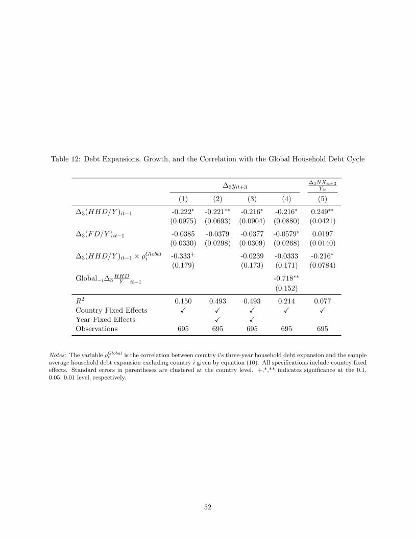
Table 12: Debt Expansions, Growth, and the Correlation with the Global Household Debt Cycle

∆3yit+3∆3NXit+3

Yit

(1) (2) (3) (4) (5)

∆3(HHD/Y )it−1 -0.222∗ -0.221∗∗ -0.216∗ -0.216∗ 0.249∗∗

(0.0975) (0.0693) (0.0904) (0.0880) (0.0421)

∆3(FD/Y )it−1 -0.0385 -0.0379 -0.0377 -0.0579∗ 0.0197(0.0330) (0.0298) (0.0309) (0.0268) (0.0140)

∆3(HHD/Y )it−1 × ρGlobali -0.333+ -0.0239 -0.0333 -0.216∗

(0.179) (0.173) (0.171) (0.0784)

Global−i∆3HHDY it−1

-0.718∗∗

(0.152)

R2 0.150 0.493 0.493 0.214 0.077Country Fixed Effects X X X X XYear Fixed Effects X XObservations 695 695 695 695 695

Notes: The variable ρGlobali is the correlation between country i’s three-year household debt expansion and the sampleaverage household debt expansion excluding country i given by equation (10). All specifications include country fixedeffects. Standard errors in parentheses are clustered at the country level. +,*,** indicates significance at the 0.1,0.05, 0.01 level, respectively.

52

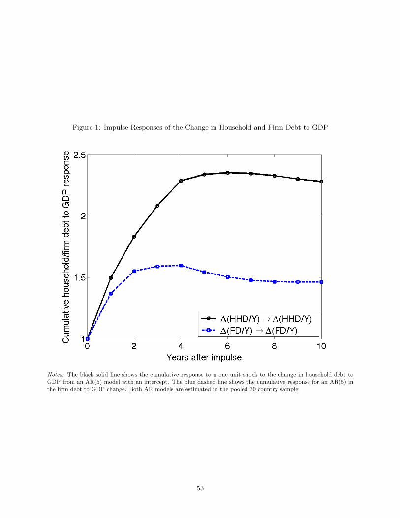
Figure 1: Impulse Responses of the Change in Household and Firm Debt to GDP

Notes: The black solid line shows the cumulative response to a one unit shock to the change in household debt toGDP from an AR(5) model with an intercept. The blue dashed line shows the cumulative response for an AR(5) inthe firm debt to GDP change. Both AR models are estimated in the pooled 30 country sample.

53

Figure 2: Three-Year Increase in Household and Firm Debt to GDP and Subsequent Growth

Notes: The figure plots {βhHH , βhF } from the following specification estimated at each horizon h: yit+h − yit =

αhi +βhHH∆3HHDit−1

Yit−1+βhF∆3

FDit−1

Yit−1+ εit. Each regression includes country fixed effects. The solid circle and square

lines plot the estimates {βhHH , βhNF }. Dashed lines represent 95% confidence intervals, computed using standard errorsclustered at the country level.

54

Figure 3: Household Debt to GDP Expansion and Growth

(a) Household Debt

(b) Household Debt, Partial Correlation (c) NF Firm Debt, Partial Correlation

Notes: This figure plots the relationship between GDP growth from t to t + 3 and the expansion in household andfirm debt to GDP from t − 4 to t − 1. Each point refers to year t. The dashed line is the non-parametric plot ofGDP growth from t to t+ 3 against the increase in household or firm debt to GDP from t− 4 to t− 1. In panels (b)household debt is partialed out with the expansion in non-financial firm debt to GDP, while in panel (c) non-financialfirm debt is partialed out with the expansion in household debt to GDP.

55

Figure 4: Estimates of βHH,i for Each Country Individually

Notes: This figure plots βHH,i from the time series regression, yit+3−yit = β0 +βHH,i∆3HHDit−1

Yit−1+∑3j=1 γj∆yit−j+

εit, estimated separately for each country i in the sample. Regressions for Ireland (IRL) and Indonesia (IDN) controlfor ∆3yit−1 instead of a distributed lag in GDP growth as a consequence of the limited degrees of freedom. Theunweighted average of the estimates refers to the raw average of the coefficients in the figure, and the precisionweighted average is the average weighted by the inverse of the squared standard error.

56

Figure 5: Responses to Household and Firm Debt to GDP Increases in a Three-Variable VAR

(a) Debt to GDP response (b) Real GDP response

Notes: This figure shows cumulative impulse responses to household and firm debt to GDP shocks from a threevariable recursive VAR in real GDP growth, the change in firm debt to GDP, and the change in household debtto GDP ,(∆ lnYit,∆(FD/Y )it,∆(HHD/Y )it). The impulse responses are from a VAR estimated on the pooled 30country sample. Dashed lines represent 68% and 95% confidence bands.

57

Figure 6: Debt Expansions and Subsequent IMF Forecasts and Forecast Errors

Notes: The left panel plots coefficient estimates from estimating: ∆hyIMFt+h|t = αhi +βhHH∆3

HHDit−1

Yit−1+βhF∆3

FDit−1

Yit−1+

εit, where ∆hyIMFt+h|t is the IMF forecast of growth from t to t + h made in year t. The right panel shows estimates

from the same equation where the dependent variable is the forecast error. Dashed lines represent 95% confidenceintervals, computed using standard errors clustered at the country level. See Table 6 for details on the IMF WorldEconomic Outlook forecasts.

58

Figure 7: Household Debt Expansion Predicts Negative GDP Growth Forecast Errors

(a) IMF World Economic Outlook Forecast Errors

(b) OECD Economic Outlook Forecast Errors

Notes: Panel (a) plots the three-year GDP forecast error from the Fall issue of the IMF World Economic Outlookagainst the change in household debt to GDP from t − 4 to t − 1. The sample includes years 1990-2012. Panel (b)plots the two-year GDP forecast error from the Fall OECD Economic Outlook against the change in household debtto GDP from t − 4 to t − 1. The sample includes years 1987-2012. We exclude Hong Kong, Indonesia, Singapore,and Thailand from the OECD sample because of gaps in the forecast series. Each point refers to year t.

59

Figure 8: Debt Expansions and Preceding IMF Forecasts

Notes: The left panel plots coefficient estimates from estimating: ∆hyIMFit−5+h|t−5 = αhi + βhHH∆3

HHDit−1

Yit−1+

βhF∆3FDit−1

Yit−1+ εit, where ∆hy

IMFt+h−5|t−5 is the IMF forecast of growth from t− 5 to t− 5 + h made in year t− 5. The

right panel shows estimates from the same equation where the dependent variable is the forecast error. Dashed linesrepresent 95% confidence intervals, computed using standard errors clustered at the country level. See Table 6 fordetails on the IMF World Economic Outlook forecasts.

60

Figure 9: Debt Expansions and Subsequent Growth Across Exchange Rate Regimes

Notes: This figure reports results from estimating the following specification separately for fixed, intermediate, and floating exchangerate regimes: ∆hyit+h = αhi + βhHH∆

HHDit−1

Yit−1+ βhF∆

FDit−1

Yit−1+∑3j=1 γ

hj ∆yit−j + εit. The left and right panels show the estimates of

βhHH and βhF , respectively, for h = 1, ...5. See Table 8 for details on classifying observations by exchange rate regime.

61

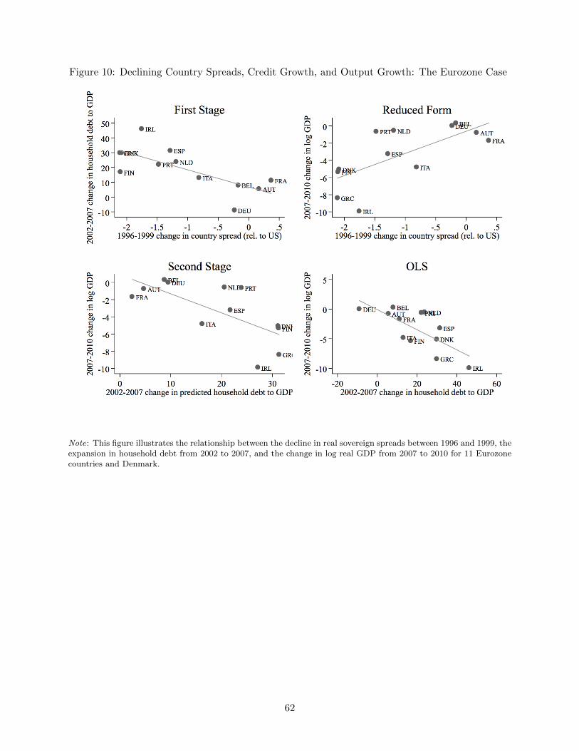
Figure 10: Declining Country Spreads, Credit Growth, and Output Growth: The Eurozone Case

Note: This figure illustrates the relationship between the decline in real sovereign spreads between 1996 and 1999, theexpansion in household debt from 2002 to 2007, and the change in log real GDP from 2007 to 2010 for 11 Eurozonecountries and Denmark.

62

Figure 11: Global Household Debt Expansions and Global Growth

(a) Household Debt

(b) Household Debt, Partial Correlation (c) NF Firm Debt, Partial Correlation

Note: This figure illustrates the relationship between the sample average of real GDP growth from t to t + 3 andthe sample average of the change in household and firm debt to GDP from t − 4 to t − 1. Each point refers toyear t. In panel (b) household debt is partialed out with the expansion in non-financial firm debt, while in panel(c)non-financial firm debt is partialed out with the expansion in household debt.

63

Figure 12: Correlation with World Household Debt Cycle

Note: This figure shows the correlation between the three-year household debt to change for country i and the average

change for all countries excluding i: corr((

∆3HHDY

)it, 1N−1

∑j 6=i(∆3

HHDY

)jt

).

64