Household Leverage and Labor Market OutcomesEvidence from a Macroprudential Mortgage Restriction

Gazi Kabaş

University of Zurich

Swiss Finance Institute

Kasper Roszbach

Norges Bank

University of Groningen

November 2021

Click here for the latest versionAbstract

Does household leverage matter for worker job search, matching in the labor market,and wages? Theoretically, household leverage can have opposing effects on the labormarket through debt-overhang and liquidity constraint channels. To test which channeldominates empirically, we exploit the introduction of a loan-to-value ratio restriction inNorway that exogenously reduces household leverage. Focusing on a sample of displacedworkers who bought a house before losing their jobs due to mass layoffs, we find thata reduction in leverage raises the subsequent wages of these workers. Lower leverageenables workers to search longer, find jobs in higher-paying firms, and switch intonew occupations and industries. The positive effect on wages is persistent and morepronounced for young and highly-educated workers who are more likely to benefit fromthe effects of a reduction in leverage on job search. Our results indicate that in additionto reducing financial stability risks, policies limiting household leverage can improveworkers’ labor market outcomes.

JEL classification: E21, G21, G51, J21.

Keywords: Household Leverage, Household Debt, Job Displacement, Job Search, Macro-prudential Policy.

Kabaş is at the University of Zurich, Institute for Banking, and Finance and Swiss Finance Institute (gazi.kabas@bf.uzh.ch).Roszbach is at Norges Bank and the University of Groningen (kasper.roszbach@norges-bank.no). The authors would like tothank Knut Are Aastveit, Konrad Adler, Yavuz Arslan, Marlon Azinovic, Scott Baker, Christoph Basten, Tobias Berg, BrunoBiais, Marco Ceccarelli, Piotr Danisewicz, Anthony DeFusco, Ahmet Degerli, Sebastian Doerr, Işıl Erel, Egemen Eren, AndreasFuster, Marc Gabarro, Thomas Geelen, Ella Getz Wold, Paul Goldsmith-Pinkham, Itay Goldstein, Knut Hakon Grini, RagnarJuelsrud, Sasha Indarte, Ankit Kalda, Andreas Kostol, Yueran Ma, David Matsa, Charles Nathanson, Dirk Niepelt, StevenOngena, Michaela Pagel, Pascal Paul, José-Luis Peydró, Ricardo Reis, Francesc Rodriguez Tous, Ahmet Ali Taskin, JoachimVoth, Toni Whited, and Jiri Woschitz, as well as participants at the CBID Central Banker’s Forum, EFiC Conference in Bankingand Corporate Finance, IBEFA Young Economist Seminar Series, Cleveland Fed, Norges Bank, University of Groningen andUniversity of Zurich for their helpful conversations and comments. Kabaş gratefully acknowledges financial support from theEuropean Research Council (ERC) under the European Union’s Horizon 2020 research and innovation programme ERC ADG2016 (No. 740272: lending). This paper should not be reported as representing the views of Norges Bank. The views expressedare those of the authors and do not necessarily reflect those of Norges Bank.

1 Introduction

Household leverage can pose a challenge for the economy through several channels. An

increase in household leverage can fuel a housing boom, predict lower GDP growth and higher

unemployment, or weaken financial stability.1 In the wake of the global financial crisis, many

countries have thus adopted policies to restrict household leverage. These policies face the

challenge of properly trading off the costs of restricting borrowing in good times against the

benefits of a less pronounced decline in bad times. Such trade-offs have sparked a debate

about the effectiveness and side effects of measures to restrict household borrowing.2 While

existing research has primarily examined the effects of household leverage restrictions on

the housing market, we instead focus on the interaction of these restrictions with the labor

market. Specifically, we study how a loan-to-value (LTV) ratio restriction policy affects the

job search and wages of displaced workers who bought a house before losing their jobs.

Theoretically, household leverage can affect the starting wages of displaced workers

through multiple channels.3 On the one hand, household leverage might increase the start-

ing wages through a debt-overhang channel. Specifically, higher household leverage directs

a larger share of wages to debt-related payments. This may reduce workers’ willingness

to work as it lowers the benefits they get from wages, leading workers to require higher

wages (Donaldson et al., 2019). On the other hand, higher household leverage may reduce

starting wages through a liquidity constraint channel. Workers with higher leverage have

larger mortgage amortization due to larger debt payments. Thus, for such workers, liquidity

constraints are more binding, which can change their preferences regarding job offers. For

1For housing booms, see Mian and Sufi (2011); Adelino et al. (2016) and Favilukis et al. (2017). Forfinancial instability, see Schularick and Taylor (2012) and Reinhart and Rogoff (2008). For economic growth,see Mian et al. (2017).

2Research has shown that these policies can improve financial stability yet create some negative side ef-fects for affected households (Farhi and Werning, 2016; Acharya et al., 2019; Araujo et al., 2019; Van Bekkumet al., 2019; Peydró et al., 2020). Tzur-Ilan (2020) and Aastveit et al. (2020) point out certain negative sideeffects that these policies may bring about. Galati and Moessner (2013) and Claessens (2015) provide athorough discussion on macroprudential policies.

3Throughout the paper, we focus on the starting wages of displaced workers in their new jobs and referto them as starting wages.

1

instance, to avoid costly defaults or keep housing consumption unchanged, workers with high

leverage may prefer earlier but certain job offers to later offers with possibly higher wages

(Chetty and Szeidl, 2007; Ji, 2021). Which of these opposing theoretical channels dominates

is ultimately an empirical question.

We estimate the effect of household leverage on job search and starting wages by exploit-

ing the introduction of an LTV restriction in Norway, which creates an exogenous variation

in household leverage. Our main finding is that a reduction in household leverage improves

the starting wages of displaced workers in their new jobs. Specifically, we show that a de-

cline in a worker’s debt-to-income (DTI) ratio by 25 percent leads to a relative increase in

starting wages by 3.3 percentage points.4 We explain our main result by documenting that

the policy-induced reduction in leverage affects workers’ job search behavior in three ways.

First, following the mandated reduction in their leverage, workers prolong their unemploy-

ment duration by approximately 2.5 months. Second, workers with lower leverage find jobs

in firms with a higher wage premium. Third, workers with lower leverage are relatively more

likely to switch to other occupations and industries, which implies that their job search reach

is broader. Furthermore, we show that the improvement in wages does not diminish over

time. Overall, our results imply that household leverage creates constraints on the job search

behavior, and a policy that restricts leverage relaxes these constraints and enables workers

to attain higher wages in their new jobs.

Studying how household leverage affects job search behavior and wages entails two em-

pirical hurdles. The first is an econometric one. Decisions on debt, job search, and job

acceptance are likely to be made jointly and may reflect heterogeneity in preferences or be-

liefs. Studying the role of workers’ household leverage in their labor market behavior thus

requires exogenous variation in their leverage that affects their job search. The second hur-

dle is the steep data requirement. Gaining a thorough understanding of how leverage affects

4We measure the household leverage by the DTI ratio. This ratio is households’ total debt divided byhouseholds’ total income before job displacement. Wages are measured at the individual (worker) level.Section 3 explains the construction of these variables.

2

workers’ labor market choices requires access to worker-level balance sheet data and granular

labor market information.

We overcome these two challenges and take a step forward in identifying the role of house-

hold leverage for labor market outcomes. We tackle the econometric challenge in two steps.

First, we make use of the introduction of a macroprudential policy that requires Norwegian

banks to put a cap on the maximum LTV ratio for home purchases, which effectively restricts

household leverage. This restriction creates exogenous variation in the DTI ratio of home

buyer workers because some of the workers would obtain a larger mortgage if this restriction

were not implemented. One feature of this restriction is that it is applied to all homebuy-

ers after 2012, when it was introduced.5 Therefore, there is no variable distinguishing the

affected workers who obtain smaller mortgages due to the restriction from the unaffected

workers who would obtain the same mortgage if the restriction were not implemented. To

make this distinction, we use the characteristics and LTV ratio decisions of workers before

the restriction. Before the restriction, mortgages could have LTV ratios above or below the

cap. This enables us to classify observations before the restriction into treatment and control

groups correctly for this period. We use these correctly classified observations and their char-

acteristics to classify our entire regression sample into treatment and control groups based

on a random forest (RF) prediction model, a machine learning method (Abadie, 2005).6,7

Therefore, our treated workers are those who are predicted to prefer high LTV ratios, before

and after the restriction, but cannot do so after the restriction; the control workers are those

who are predicted to prefer low LTV ratios whether or not the restriction is in place.

Second, we restrict the worker sample to displaced workers to limit the effect of individual

characteristics on job search. The displaced workers lost their jobs due to a mass layoff–a

5A small number of mortgages are exempted; see Section 2.26Van Bekkum et al. (2019); Aastveit et al. (2020) have a similar strategy in an LTV ratio restriction

setting.7We train and validate the RF model with all first-time homebuyers before the implementation except

for those in the regression sample. Then, we use this trained RF classifier for the entire regression sample.Section 4.1 explains the implementation of RF prediction model in detail.

3

case in which a firm reduces its workforce by at least 30 percent in a given year. Therefore,

the job search of these workers is not triggered by individual characteristics. Furthermore to

reduce heterogeneity in accumulated home equity prior to the layoff, we restrict our sample

to those displaced workers who bought a house within 12 months prior to their displacement.

We tackle the steep data requirement with the help of several population registers avail-

able in Norway. First, we obtain debt, income, and other balance sheet data from the official

tax filings for the entire adult population of Norway. Then, we merge these tax data with

information from the national Register of Employers and Employees, to which all employers

and contractors are obliged to report their workers and freelancers, as well as the details of

the employment relationship. Finally, we complement this with home purchases collected

by the Norwegian Mapping Authority. This unique data set includes information about

individuals’ assets and liabilities, wages, unemployment duration, job choice, and other in-

dividual characteristics such as education and immigration status. We use this data set

to conduct a difference-in-differences analysis, comparing those displaced workers who had

recently bought a house and are likely affected by the LTV restriction (treatment group) to

those who are not affected by the restriction (control group). We obtain three main results.

First, upon introduction of the LTV ratio restriction, the treated workers experience a

drop in their household leverage. More specifically, the restriction reduces these treated

workers’ DTI ratios by 25 percent. This decline in the DTI ratio is realized by means of a

reduction in the mortgage size and a downward adjustment in the price of acquired homes.

Thus, these findings indicate that the LTV restriction was highly effective in constraining

borrowing by households, and therefore provides an excellent experimental setting to investi-

gate the implications of household leverage on job search behavior and related labor market

outcomes.

Second, using the decline in household leverage caused by the LTV ratio restriction,

we identify the effect of leverage on the labor market outcomes of displaced workers who

4

recently bought a house before their displacement. We show that affected workers with

reduced leverage manage to realize higher wage growth between the job from which they

are displaced and the next job they find. In particular, we find that a 25 percent decline in

workers’ DTI ratio leads to a 3.3 percentage point smaller decline in wages compared to the

7.4 percentage point average reduction after a displacement. The improvement in starting

wages is robust to controlling for individual, location, and industry-specific characteristics,

refining the worker sample by removing workers with a possibly different attachment to the

labor market, narrowing down the sample by gradually excluding observations below the

restriction threshold, and controlling for macroeconomic conditions.

More importantly, we show that the effect of leverage on starting wages is not driven by

endogenous selection into the housing market. The LTV restriction can directly affect house

purchase decisions. Households that cannot afford the down payment can try to buy their

houses before implementation of the LTV restriction. Alternatively, such households can

delay their purchase until they can afford the down payment. Due to endogenous selection

into the housing market, the treated workers may have different characteristics before and

after the restriction, which can partially drive our results. We mitigate this selection concern

in two ways. First, we show that the LTV restriction does not change the observable char-

acteristics of the treated workers. Second, we restrict our sample to those who are able to

afford the down payment, both before and after the restriction. Because the main reason for

endogenous selection is the ability to afford the down payment, this restricted sample does

not suffer from the selection concern. Our estimates obtained from this restricted sample

are remarkably close to our main results, which strongly suggest that our results are not

confounded by selection effects.

Third, we document that the improvement in starting wages stems from a reduction in

constraints in the job search that higher leverage creates. This relaxation in the constraints

influences starting wages positively through several channels. After the reduction in their

leverage, workers are able to stay as unemployed for 2.5 months longer, which suggests that

5

lower debt reduces the pressure on displaced workers to quickly find and accept a new job.

Moreover, the reduction in leverage enables displaced workers to search for job matches with

firms that pay higher wages. Following Abowd et al. (1999), we estimate firm wage premiums

using the whole Norwegian population and establish that treated displaced workers find jobs

at firms that pay higher wage premiums, which explains 20 percent of the gain in starting

wages. A reduction in leverage also enables workers to broaden the scope of their job search.

Workers with lower leverage are around 20 percent more likely to change their occupation

at a new employer and/or find a new employer in another industry. Our results show that

changes in geographical labor mobility or investment in additional education are not a drivers

of our results.

We support the mechanism by documenting how heterogeneity across the sample affects

the positive effect of reducing household leverage. If a reduction in leverage improves work-

ers’ starting wages through improved job search, we may expect to find greater gains for

subsamples who have more potential to benefit from a better job search. We find that work-

ers younger than the median age, having a shorter job tenure with the previous employer or

with higher education, drive the improvement in starting wages. This is consistent with the

notion that it is easier for younger workers or workers with higher education to invest in the

human capital required for a different occupation or industry. Longer previous job tenure

with the same firm also tends to make human capital more firm-specific and limit the value

of a better job search. In addition, further heterogeneity tests indicate that the improvement

in starting wages is particularly larger for female and low-income workers. These findings

imply that a reduction in household leverage and related improvements in the job search

may be important for disadvantaged workers in the labor market.

Finally, we find that the positive impact of lower leverage on starting wages is persistent.

Four years after their displacement, workers with reduced leverage are able to maintain a

significant wage advantage thanks to the LTV restriction. More specifically, these workers

have a 4.7 percentage point higher wages at the end of the four-year post displacement period

6

that we observe. These same workers also enjoyed lower wage volatility during the four years

after their displacement, indicating that the rise in wages is not attributed to these workers

taking jobs with greater hour volatility or a greater risk for discontinuation.

In sum, our paper documents the constraints that household leverage creates in the job

search of displaced workers and a reduction in these constraints improves these workers’ start-

ing wages. Our results thus imply that macroprudential policies aiming to limit household

leverage can have positive side effects for the labor market. One concern of such macropru-

dential policies is that, due to the down payment requirement they introduce, these policies

can delay households’ house purchases, thereby imposing utility costs on affected households.

We show that owing to macroprudential policies, these households may have better prospects

in the labor market. In addition, our results provide new insights on how household lever-

age interacts with the economy. These new insights on the labor market implications of

household leverage might be particularly important for policymakers. Considering that high

household leverage is one of the common characteristics of recent recessions, policymakers

may find themselves coping with the negative consequences of household leverage during

these recessions.

The findings in our paper speak to at least four strands of the literature. First, our paper

adds to the literature showing that household debt and credit access affect labor markets

through a demand channel. This channel starts with the negative effect of household leverage

on credit availability. This negative effect can occur due to the detrimental effect of leverage

on financial stability (Reinhart and Rogoff, 2008; Schularick and Taylor, 2012; Corbae and

Quintin, 2015), or on collateral values (Adelino et al., 2016). The decline in credit availability

may entail deleveraging by households. Due to the required deleveraging, households may

need to cut their spending (Eggertsson and Krugman, 2012; Mian et al., 2013; Guerrieri

and Lorenzoni, 2017), which in turn puts pressure on the aggregate demand and increases

unemployment (Mian and Sufi, 2014; Mian et al., 2017). Our findings complement these

analyses by documenting the direct effect of household leverage on the labor markets. In

7

addition to the indirect demand channel, household leverage affects workers’ job search and

labor market outcomes by introducing constraints that reduce the matching quality in the

labor market.

Second, our paper is related to the literature studying the determinants of the labor

supply and job search. Unemployment insurance and severance pay are considered to be the

main determinants of the labor supply of the unemployed.8 Bernstein and Struyven (2017);

Brown and Matsa (2019); Bernstein (2020) and Gopalan et al. (2020) document how negative

home equity following from a decline in house prices hurts labor mobility and labor supply.

Liquidity constraints (He and le Maire, 2020; Kumar and Liang, 2018), credit access during

unemployment (Herkenhoff, 2019), mortgage payments (Zator, 2019), and wealth shocks

(Cesarini et al., 2017; Bernstein and Koudijs, 2021) also influence individual labor supply

decisions.9 We contribute to this growing literature in three ways. First, we document that,

in addition to the aforementioned variables, household leverage is an important determinant

of the job search.10 This contribution complements existing work by providing new insights

in the following way. The positive effect of access to credit and mortgage payments on wages

documented by earlier papers suggests a positive effect of household leverage on wages as

well, given that household leverage is positively correlated with access to credit and mortgage

payments. However, contrary to this suggestion, we find a negative effect of leverage on

wages, which improves our understanding on how household leverage interacts with the

economy in general. Our second contribution is that we focus on displaced workers who

lost their jobs due to mass layoffs, instead of the whole population or all home buyers. Our

sample design allows us to cleanly estimate changes in the wages and job search as the job

8The relation among unemployment insurance, severance payments, and the labor supply has beenstudied extensively. See Lalive et al. (2006); Chetty (2008); Rothstein (2011); Card et al. (2007) and Bastenet al. (2014).

9See also Mulligan (2009, 2010); Li et al. (2020) and Cespedes et al. (2020). Rothstein and Rouse (2011)find that student debt affects students’ academic decisions, causes graduates to choose higher-salary jobs atthe cost of taking fewer lower-paid “public interest” jobs. Sharing negative information about households’past credit market behavior has also been shown to reduce employment and mobility (Bos et al., 2018).

10Bednarzik et al. (2017); Meekes and Hassink (2019); and Fontaine et al. (2020) document correlationsbetween household balance sheets and labor market outcomes.

8

search behavior of the displaced workers is not triggered by any individual characteristics.

Third, using detailed individual labor market data, we can lay bare the exact mechanisms

through which changes in the job search affect wages. This allows us to measure the influence

of job search on the starting wages.

Third, our paper contributes to discussions on how macroprudential policy tools are

affecting the economy by investigating the influence of an LTV ratio restriction, one of the

most popular macroprudential tools, on the labor markets. On the one hand, these policy

tools can curb credit booms and improve financial stability (Borio, 2003; Igan and Kang,

2011; Claessens et al., 2013; Cerutti et al., 2017; Van Bekkum et al., 2019; Defusco et al.,

2019; Araujo et al., 2019; Peydró et al., 2020).11 On the other hand, these tools can generate

some negative unintended side effects (Acharya et al., 2019; Aastveit et al., 2020; Tzur-Ilan,

2020). We document an additional but positive unintended effect for an LTV ratio restriction

on the labor markets. Having a similar research question to ours, Pizzinelli (2018) develops a

life-cycle model with LTV and LTI restrictions to study second earners’ labor supply. While

Pizzinelli (2018) does not find any effect of an LTV restriction on female employment in his

model, we empirically document that, by reducing household leverage, the LTV restriction

increases displaced workers’ starting wages.

Fourth, our paper adds to the research investigating the consequences of job displacement.

This literature has found that the decline in earnings after being displaced can be large

and long-lasting (Jacobson et al., 1993; Couch and Placzek, 2010; Davis and Von Wachter,

2011; Lachowska et al., 2020) and depend on the business cycle and employer characteristics

(Schmieder et al., 2018; Moore and Scott-Clayton, 2019).12 We contribute to this literature

by demonstrating that policy-induced reductions in household leverage can mitigate the loss

11See Farhi and Werning (2016) and Dávila and Korinek (2018) for theoretical justifications for macro-prudential policies.

12The decline in earnings after a mass layoff is not age-dependent (Ichino et al., 2017). Halla et al. (2020)show that intra-household insurance may not be sufficient to cover this income loss. Losing one’s work ina mass layoff also affects the private sphere through increased mortality and divorce rates (Charles andStephens, 2004; Sullivan and von Wachter, 2009).

9

of income following a job loss.

The rest of the paper is organized as follows: Section 2 provides information about

economic conditions in Norway, Section 3 describes the data and variables constructed,

Section 4 explains the empirical strategy, Section 5 presents the impact of LTV constraint

on household finances and labor market outcomes, and Section 6 concludes.

2 Institutional background

2.1 The Norwegian economy

Norway’s economy has displayed stable economic growth, with both inflation and average

unemployment below four percent during the past 30 years. During the Global Financial

Crisis (GFC) GDP fell by only 1.7 percent. During the full sample period, Norges Bank’s

policy rate varied between 5.75 and 1.25 percent (Figure A1). As shown in Figure 1a house

prices have nearly tripled since 2000. Norwegian households’ debt to GDP ratio has simul-

taneously increased from 50 percent to 105 percent (Figure 1b). The home ownership rate

in Norway is above 80 percent and among the highest in advanced countries. Nine out of

ten mortgages have a floating interest rate. Mortgages are full-recourse.

2.2 Macroprudential policy

Norway is not a member of the EU but has committed to implementing the relevant EU

financial sector directives through the EEA-agreement. The main legal basis for regulating

financial institutions and credit markets is the Financial Institutions Act (Lov om Finans-

foretak og Finanskonsern, henceforth FIA) which has been in effect since 1 January 2016. In

Norway, the main responsibility for financial stability lies with the government, and the Min-

istry of Finance has been the designated macroprudential authority since 2016. The financial

10

stability instruments are shared among the Ministry of Finance (MoF), the Finanstilsynet

(Financial Supervisory Authority–FSA) and Norges Bank (Central Bank of Norway). While

the FSA advises the MoF on desirable regulations under the FIA, decisions on new regula-

tions are made by the Ministry.

The steep rise in house prices and household indebtedness and possible spillover effects

on financial stability raised concerns with the Norwegian policymakers already before 2010.

To reduce households’ vulnerability and banks’ exposure to housing markets, the FSA issued

"Guidelines for prudent lending standards for new residential mortgage loans" in both 2010

and 2011. The March 2010 guidelines established a maximum permissible LTV ratio of

90 percent. Compliance with the new guidelines was expected by fall 2010. Through the

December 2011 update, the FSA reduced the LTV to 85 percent and specified that mortgages

granted on the same property by other lenders shall also be included in the LTV ratio.13

Interest-only mortgages and collateralized lines of credit were restricted by an LTV ratio of

70 percent. The guidelines permitted banks to deviate from the target ratios if borrowers

could pledge additional collateral or the bank performed a special prudential assessment.

The guidelines further specified that each lender’s board of directors was responsible for

establishing criteria for the special prudential assessments and taking action on any deviation

from the guidelines. Financial institutions were instructed to immediately start incorporating

the guidelines in their internal guidelines.14 In our analysis, we focus on the joint effect of

the two LTV restrictions and consider 2012 the first year in the post-period, while excluding

2010 from the pre-period.

13The motivation for the update was that "the proportion of residential mortgages with a high loan-to-value ratio is on the increase, and a round of inspections of mortgage lending practice at a selection of banksshows that credit assessments need to improve." See Finanstilsynet (2011)

14In July 2015, after adoption of the FIA, the MoF converted the guidelines into a regulation (Ministryof Finance, 2021).

11

2.3 Labor market regulation

The labor market in Norway is governed by the Working Environment Act and the Labor

Market Act, both of 2005.15,16 The Working Environment Act sets standards for working

conditions and process rules that need to be followed when an employer wishes to termi-

nate an employment relationship. Norwegian law recognizes a special status for collective

redundancies, i.e., situations where notice of dismissal is given (a) to at least 10 employees

within a 30 day period (b) without grounds related to the individual employees. An employer

contemplating collective redundancies needs to start consultations with employees’ elected

representatives at the earliest possible opportunity. The notification period for job termi-

nation depends on the employee’s job tenure and age and can range from a minimum of 30

days up to six months.17

Unemployment benefit coverage in Norway approximately equals the OECD average of

60 percent. Displaced workers can receive 62.4 percent of their previous income up to six

times the National Insurance Scheme’s basic amount for a period of 52 or 104 weeks. In

2010 the annual basic amount was NOK 75,641 (USD 12,712), compared to NOK 101,351

(USD 11,852) in 2021. Employees needed to earn at least 1.5 times the basic amount over

the previous 12 months or on average more than three times the basic amount over the

past 36 months to be eligible for unemployment benefits.18 To be entitled to the maximum

of 104 weeks of unemployment benefits a person had to earn income of at least twice the

basic amount during the previous 12 months or twice the basic amount on average during

the previous 36 months. In 2010, an employee thus had to earn at least NOK 151,282

(USD 25,425) to be eligible for two years of unemployment benefits. No person could receive

15Act relating to working environment, working hours and employment protection.16Lov om arbeidsmarkedstjenester.17The shipping, hunting and fishing, military aviation and public service sectors are excluded from the

Working Environment legislation.18The Norwegian Labour and Welfare Administration (NAV), disregards any income above six basic

amounts per period of 12 months

12

annual unemployment benefits in excess of NOK 238,199.19 The law requires people to be an

active job seeker and to inform the Norwegian Labour and Welfare Administration (NAV)

office about ongoing job search activity every fortnight. If a person cannot search for a job

search due to illness or other circumstances, benefits can be reduced or discontinued. Most

importantly for our purposes, the unemployment benefits scheme did not change during our

sample period.

3 Data and sample construction

We combine several official Norwegian population registers. Each data set covers the entire

adult population of Norway and we link the data sets with a unique, anonymized, personal

identifier. We introduce the data sets below and describe how we construct our sample and

variables.

3.1 Data sets

We obtain the labor market data for our study from the official employer-employee register

(Aa registeret) administered by NAV. All employers and contractors are obliged by law to

report their employees and freelancers as well as details on the employment relationship. In

this register, we can track for which employer an employee works, what occupation she held,

what wages were paid, the job start and termination dates, as well as the geographic location

of the workplace. We complement this labor market information with administrative data

from the population register as well as official tax records. The population register includes

background variables such as gender, age, parent identifiers, marriage status, residential

municipality, immigration status, and education. The tax records enable us to isolate labor

income and business income, capital gains, interest expenses, government transfers, debt,

1962.4 percent of six times the National Insurance Scheme basic amount (NOK 75,641)

13

bank deposits, and total wealth. The last data set is collected by the Norwegian Mapping

Authority and contains information on all real estate and housing transactions, including

both the seller and the buyer, the transaction value, and a location identifier.

3.2 Sample construction

Our main sample period starts in 2006 and ends in 2013.20 We analyze workers who have

experienced both an exogenous change in their leverage and who were displaced during the

sample period due to a mass layoff. From the full Norwegian population, we therefore draw

workers who satisfies two criteria: (a) job loss due to a mass layoff, (b) bought a house

before the job loss. To avoid a bias that an unobserved ability to building up home equity,

we restrict our sample to workers who bought their homes no more than 12 months before

their displacement.

Mass layoffs provide an appropriate setting for our research because they trigger job

displacement exogenously, i.e., job displacement that is not caused by worker-specific char-

acteristics (Flaaen et al., 2019). We define a mass layoff as a situation where a firm parts

with at least 30 percent of its workers in a year or ceases its operation entirely. We follow

the literature (Lachowska et al., 2020; Von Wachter et al., 2009; Sullivan and Von Wachter,

2009) and use only firms with at least 50 employees to limit the risk that we mistake laying

off smaller numbers of workers for idiosyncratic reasons for a mass layoff. Applying the

above two criteria yields us 1880 workers who are displaced between 2006 and 2013 from 564

different firms.

20Because of a change in the enforcement of data reporting standards, we have excluded employment datafrom 2014 and onward. Before 2014 reporting workers and labor contract data at the branch or head officewas performed by NAV. The 20014 reporting change generates noise in the data because of large numbersof "intra-group" job changes.

14

3.3 Variable construction

In this project, we use variables on two levels. Since the LTV ratio restriction applies to debt

at household level, we use the household as the unit of observation for variables that matter

for the policy, i.e., household leverage. We also measure deposits, income, and interest costs

at household level. When considering labor market outcomes and job search behavior, we

switch to the individual (worker) level. In this part of the paper, we introduce the main

variables we use and provide summary statistics in Table 1.

Due to Norway’s lack of a credit registry during our sample period, we cannot disentangle

mortgage credit from other loans using a credit type identifier. We therefore infer the LTV

ratios by using official tax register data. All Norwegian banks report individual data on

debt, deposits and interest received and paid to the Norwegian Tax Administration for the

purpose of producing pre-filled personal tax filings. By checking the Mapping Authority’s

register, we can identify people who did not own (part of a) house in the previous year. To

reduce the influence of the existing debt on LTV ratio calculation, we define mortgage credit

as the increase in the households’ total debt in the year of the home purchase. We divide the

imputed mortgage debt by the house transaction value observed in the Mapping Authority’s

housing transaction register. This means we will slightly overestimate the LTV ratio if a

household takes an additional unsecured loan or increases its utilization of an existing line

of credit in the year of the home purchase. The average of LTV ratio is 92% in our sample.

Unlike the LTV ratio, we can measure the DTI ratio exactly as the tax filings provide exact

information about the total debt and total income. We calculate the DTI ratio by dividing

household’s total debt to household’s total income before the mass layoff. The average value

of this ratio is 4.24 in our sample with a standard deviation of 2.10.

To assess the impact of the LTV ratio restriction on the starting wages of the displaced

workers, we use the wage growth between the job that workers are displaced from and the

next job that they find as the wage variable. We follow the literature and use the symmetric

15

growth rate to allow for labor market exit and limit the role of outliers.21 In line with the

job displacement literature, the average wage growth for displaced workers is negative in

our sample. Our data set allows us observe the job start and job end dates. Using these

dates, we measure the unemployment spell as the number of days between the two jobs. On

average, the displaced workers experience an unemployment spell of 132 days in our sample.

To measure education, we use the Norwegian Standard Classification of Education at the

3-digit level. Our education variable captures both the level and the broad field of education.

The level indicates if a person has compulsory, intermediate, or higher education. The broad

field refers to a general classification of the academic content. There are 142 unique education

levels in our sample.22 To capture changes in profession, we use Statistics Norway’s seven-

digit occupational information that builds on the EU’s ISCO-88 (COM) (Statistics Norway,

1998) four-level classification system. The first digit defines 10 major groups that combine

broad professions and inform about the level of competence.23 The remaining digits break

down each main occupational category into further subgroups.

Of the workers in our sample, 15 percent reside in Oslo, close to the city’s population

weighting in Norway. Roughly half of our sample was displaced from firms in the services

industry, while the remaining half is evenly distributed among the other industries.

21We follow Davis et al. (1998) and compute the symmetric growth rates as

wit =(wit − wit−1)

0.5× (wit + wit−1)(1)

22The levels are primary, lower secondary, upper secondary, post-secondary, first stage of higher education,and second stage of higher education. The broad fields are humanities and arts, teacher training andpedagogy, social sciences and law, business administration, natural sciences, health, primary industries, andtransport and communications. As an example, with 3-digit detail, we can differentiate whether a personwith social sciences and law background studies in sociology or psychology.

23The upper ten classes are (1) legislators, senior officials and managers, (2) professionals, (3) techniciansand associate professionals, (4) clerks, (5) service workers and shop and market sales workers, (6) skilledagricultural and fishery workers, (7) craft and related trades workers, (8) plant and machine operators andassemblers, (9) elementary occupations, and (10) armed forces and unspecified

16

4 Empirical strategy

Our objective is to causally identify the effect of household leverage on households’ job

search behavior and labor market outcomes. Because debt and labor choices are likely to be

made jointly, merely regressing labor market outcomes on household leverage will potentially

yield a biased estimate of the coefficient on leverage. For instance, an employee with low

labor skills that are not observed by the econometrician might assume higher debt since

due to lower skills she relies on debt to sustain consumption. In addition, these lower labor

skills could decrease the starting wage of this employee, which creates a spurious correlation

between indebtedness and wages. We address this endogeneity challenge by exploiting the

legally imposed LTV restriction as a source of exogenous variation in household leverage.

4.1 Using macroprudential policy as an experiment

The FSA issued its first mortgage guidelines in 2010 and shortly afterward updated them in

2011. In our analysis, we use the date of the 2011 guidelines as the timing of the policy exper-

iment. The initial 2010 guidelines proved to be ambiguous about the precise implementation

period, and the FSA reported low compliance with the policy (Finanstilsynet, 2011). The

updated guidelines are stricter and cover loans with collateral claims on a particular prop-

erty from all lenders. In our main regressions, we therefore remove all observations between

the two guidelines and let the post-treatment period start in 2012. Thanks to the absence

of other regulations or policy changes that could affect labor markets, the LTV restriction

policy provides a clean experimental setting in which we can study the impact of household

leverage on labor markets.

One important feature of this LTV restriction policy is that it covers the whole population.

Therefore, all observed LTV ratios are below the threshold after the policy.24 However, this

24There are few households whose LTV ratios are larger than the threshold after the policy. The reasonis that lenders could grant loans with LTVs in excess of 85 percent if additional collateral was pledged or aspecial prudential assessment was performed. Anecdotal evidence indicates that collateral pledged by parents

17

does not mean that every household is treated by the policy. The reason is that 35 percent

of the population obtains mortgages with LTV ratios lower than the threshold before the

policy, which implies that without the policy, approximately one-thirds of the households

would obtain mortgages with LTV ratios lower than the threshold. These households are

natural candidates for the control group. However, there is not a single variable that allows

us to separate these households from the treated ones.

The common solution the literature applies to similar cases where the treatment status is

missing after the policy is proxies the treatment status with one variable which is positively

correlated with the treatment.25 Facing a similar problem, recent papers on the effects

of LTV restrictions follow Abadie (2005) and use linear probability prediction models to

construct the treatment groups (Van Bekkum et al., 2019; Aastveit et al., 2020). In our

paper, we take a step forward and use machine learning (ML) methods. More specifically,

we use random forest (RF) method to classify households into treated and control groups.

Using an RF to proxy the treatment status comes with three main advantages. The

first advantage is that by using many variables instead of a single variable, RF improves

the accuracy of the treatment classification. This advantage is intuitive since a rich set of

variables has more information compared with a single variable. Athey and Imbens (2019);

Calvi et al. (2021) discuss how beneficial ML methods can be for the cases similar to ours.

The second advantage is that unlike linear probability models, RF does not impose any

functional form to the classification. Therefore, RF is capable of capturing the true data

generating process better. Third, given that RF is designed to maximize out-of-sample

forecast power with enough power to avoid overfitting, RF’s classification is more robust for

post-treatment period and inclusion of many variables.

is the most common justification for a higher LTV. Since these households do not experience a change in theirleverage and thus untreated, we remove these few observations from our estimation sample. The placebotest in Section 5.2 show that this removal does not create a bias in the wage growth regressions.

25For instance, He and le Maire (2020) use previous liquidity to construct the treated and the controlgroups.

18

We use RF to classify the households as treated and control units in three steps.26 In

the first step, we collect a rich set of household-level data from the period between 2002 and

2010. The variables in this data set include household-level income, wage, deposits, DTI,

business income, education, age, location, and immigration status. Moreover, we add par-

ents’ deposits, debt, wealth, education, and immigration status to the data.27 To incorporate

the influence of the macroeconomic conditions and house prices, we use GDP, inflation, un-

employment, monetary policy rate, and regional and national house prices. Since there is no

restriction for LTV ratios in this time period, we label the households with LTV ratio above

the threshold as treated and the others as control.28 In the second step, we use unconstrained

treatment status and the variables from the first step to estimate the model’s parameters.29.

In the last step, we classify the households in the regression sample into treated and control

groups using the trained RF model.

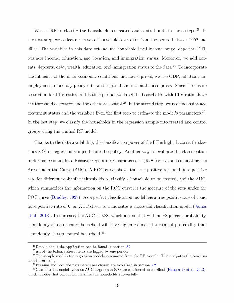
Thanks to the data availability, the classification power of the RF is high. It correctly clas-

sifies 82% of regression sample before the policy. Another way to evaluate the classification

performance is to plot a Receiver Operating Characteristics (ROC) curve and calculating the

Area Under the Curve (AUC). A ROC curve shows the true positive rate and false positive

rate for different probability thresholds to classify a household to be treated, and the AUC,

which summarizes the information on the ROC curve, is the measure of the area under the

ROC curve (Bradley, 1997). As a perfect classification model has a true positive rate of 1 and

false positive rate of 0, an AUC closer to 1 indicates a successful classification model (James

et al., 2013). In our case, the AUC is 0.88, which means that with an 88 percent probability,

a randomly chosen treated household will have higher estimated treatment probability than

a randomly chosen control household.30

26Details about the application can be found in section A2.27All of the balance sheet items are lagged by one period.28The sample used in the regression models is removed from the RF sample. This mitigates the concerns

about overfitting.29Pruning and how the parameters are chosen are explained in section A2.30Classification models with an AUC larger than 0.90 are considered as excellent (Hosmer Jr et al., 2013),

which implies that our model classifies the households successfully.

19

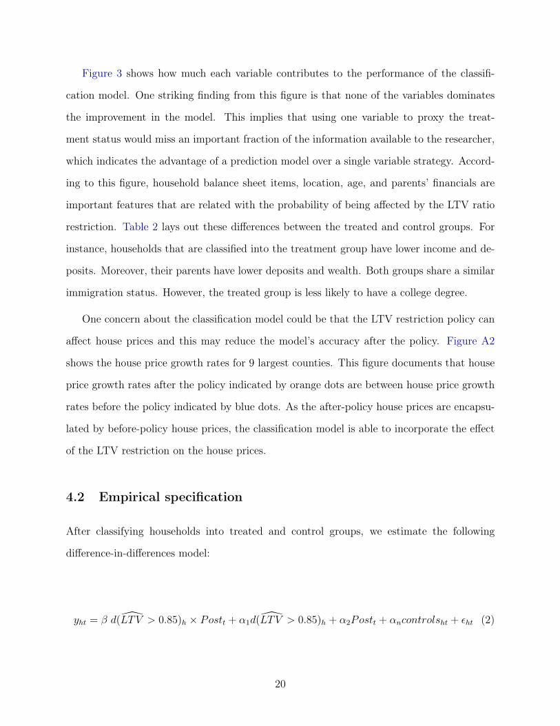
Figure 3 shows how much each variable contributes to the performance of the classifi-

cation model. One striking finding from this figure is that none of the variables dominates

the improvement in the model. This implies that using one variable to proxy the treat-

ment status would miss an important fraction of the information available to the researcher,

which indicates the advantage of a prediction model over a single variable strategy. Accord-

ing to this figure, household balance sheet items, location, age, and parents’ financials are

important features that are related with the probability of being affected by the LTV ratio

restriction. Table 2 lays out these differences between the treated and control groups. For

instance, households that are classified into the treatment group have lower income and de-

posits. Moreover, their parents have lower deposits and wealth. Both groups share a similar

immigration status. However, the treated group is less likely to have a college degree.

One concern about the classification model could be that the LTV restriction policy can

affect house prices and this may reduce the model’s accuracy after the policy. Figure A2

shows the house price growth rates for 9 largest counties. This figure documents that house

price growth rates after the policy indicated by orange dots are between house price growth

rates before the policy indicated by blue dots. As the after-policy house prices are encapsu-

lated by before-policy house prices, the classification model is able to incorporate the effect

of the LTV restriction on the house prices.

4.2 Empirical specification

After classifying households into treated and control groups, we estimate the following

difference-in-differences model:

yht = β d(LTV > 0.85)h × Postt + α1d(LTV > 0.85)h + α2Postt + αncontrolsht + εht (2)

20

where yit is either household balance sheet variables such as debt-to-income ratio or labor

market variables such as wage growth. d(LTV > 0.85)h is a dummy variable that takes the

value of 1 if a household is predicted to have an LTV ratio larger above the threshold. We

saturate the difference-in-differences model with year, education, location, and industry fixed

effects. Given that our sample consists of people who are displaced in mass layoffs, which

may be driven by developments at the industry and/or location level, we double cluster the

standard errors at the industry and location level (Abadie et al., 2017). Moreover, we use

Murphy-Topel standards errors as we use predicted regressors (Murphy and Topel, 1985).

The main identifying assumption underlying the model in Equation 2 is that the outcome

variables of treated and control groups would have parallel trends if the policy weren’t

implemented. The standard way to test this identifying assumption is to look the trends

of the treated and control groups before the treatment. A confirmation that the trends

are parallel provides strong support for the assumption that, absent treatment, treated and

control groups would have experienced similar paths in their outcomes. We investigate the

trend differences in the pre-treatment period by estimating the following model:

yht =2∑

k=−4

γk Dk × d(LTV > 0.85)h + d(LTV > 0.85)h + αncontrolsht + εht (3)

where we replace postt with period dummies. Since we omit period = −1 in Equation 3,

the estimated γk coefficients document the difference between treated and control groups at

period = k relative to that of at period = −1.

Our construction of the treated and control groups has two implications. First, we may

incorrectly classify the treatment status. Lewbel (2007) documents that misclassification

of a binary regressor creates an attenuation bias, akin to standard measurement error bias.

This implies that our parameter estimates, if misclassification were an issue, will provide

a lower bound for the effect of household leverage on labor market outcomes. The out-

of-sample predictive power of our RF model being above 80 percent provides additional

21

reassurance about the risk of misclassification. Moreover, as depicted in Figure A3, majority

of the misclassified households are clustered around the threshold.31 The impact of the LTV

policy on household leverage is smaller for the households whose LTV ratios are closer to the

thresholds since the policy reduces the leverage with a smaller amount. Therefore, having

majority of the misclassified households clustered around the threshold suggests that the

magnitude of the attenuation bias is limited. Second, since we use several proxy variables

to assign households to the treated or control group, the groups are likely to differ along

these variables. These differences can lead to different labor market outcomes without an

exogenous change in household leverage.32 While the proxy variables are allowed to affect

the levels of the labor market outcomes, the above procedure rests on the assumption that

the proxy variables do not affect the change in labor market outcomes. This rules out the

possibility that the influence of these proxy variables on labor market outcomes changes at

the same time as the LTV restriction is introduced. Parallel trends graphs in Section 5 make

it clear that the difference in labor market outcomes between the treated and control groups

are stable before the introduction of the LTV restriction, which confirms that there is no

change in levels of labor market outcomes in this time period.

5 Impact of the LTV restriction

Our analysis builds on the fact that a macroprudential policy aimed at reducing households’

ability to borrow against collateral creates an exogenous reduction in affected households’

indebtedness. The immediate effect of the macroprudential policy was to limit households

LTV ratios. In Section A1 we document that the LTV restriction is well-behaved and affects

the LTV, balance sheet components, interest payments and the value of purchased houses

in line with expectations. In this section we start by detailing the direct effect of the policy

31Note that before the implementation of the restriction, we observe both the realized and predictedtreatment status.

32Our regression results in Section 5 indicate that treated households have lower starting wages beforethe LTV restriction.

22

on households leverage, measured as the DTI ratio, in Section 5.1. Section 5.2 describes the

impact of the policy on wages while section 5.3 lays out the mechanism through which lower

leverage affects wages and other labor market outcomes. Section 5.4 contains estimates of

the longer term effects of the policy.

5.1 Impact of LTV restriction on household leverage

We expect the LTV restriction to limit affected households indebtedness. To provide visual

evidence of how the LTV restriction reduces household DTI ratio, we estimate Equation 3

with the DTI ratio as the dependent variable. Figure 5 depicts the estimated coefficients.

The difference between the DTI ratios of treated and control groups is essentially constant

during the pre-treatment period, which lends support to the underlying assumption that the

DTI ratios of the two groups would follow parallel trends in the absence of the restriction.

After the restriction, the treated group has substantially lower leverage. Table 3 displays

the parameter estimates from the corresponding difference-in-differences model (Equation 2)

of Section 4 and confirms the implications of Figure 5. In the baseline regression without

any fixed effects, the LTV restriction reduces treated households’ DTI by 109 percentage

points. In column (2), we include year fixed effects to control for time effects, and we further

saturate the model with education fixed effects in column (3).

A potential concern about our model specification could be that mass layoffs may not

occur randomly, which could bias our parameter estimates. To tackle the concern that layoffs

may occur due to location or industry specific shocks, we also include location, industry, and

location×industry fixed effects in Columns (4)-(6) to control for the selection problem that

unobservables might generate. In all specifications, d(LTV > 0.85)h × Postt has a highly

significant and negative coefficient that is quantitatively close to the estimate from the model

without any fixed effects. The LTV restriction thus reduces treated households’ leverage by

on average 105 to 115 percentage points, which is 25 percent decline at the mean value.

23

In Section A1, we further document how the restriction reduces household leverage.

Treated households take on smaller mortgages, which they use to buy cheaper houses. We

find that they, after introduction of the policy, take on mortgages that are on average NOK

603,000 smaller to pay for homes that are NOK 503,000 cheaper. According to our esti-

mations, the restriction reduces households’ liquidity, however, the estimated effect is not

statistically significant. We complement these findings by showing that the LTV restric-

tion also eases the interest expenses of treated households. This decline in interest expense

and lower principal repayment expenses, thanks to smaller mortgages, together cut the cash

outflow by approximately 10 percent of the household’s wages before displacement.

5.2 Impact of household leverage on starting wages

After establishing the negative impact of the LTV restriction on household leverage, we next

investigate how household leverage affects displaced workers’ starting wages from their new

employers. In principle, household leverage can have opposing effects on starting wages. On

the one hand, it can create a debt overhang problem that lowers displaced workers’ appetite

to work since a larger fraction of earnings will go to their lenders. To attract workers, firms

then have to post vacancies with higher wages (Donaldson et al., 2019). Therefore, this

mechanism predicts that displaced workers with high household leverage find jobs with higher

wages. On the other hand, household leverage can reduce the starting wages of the displaced

workers. For instance, in one channel, household leverage creates pressure on displaced

workers because they need to service their debt (Ji, 2021). The reason is that defaulting on

loans has been shown to be associated with substantial costs such as deteriorated credit scores

or worsened labor market prospects.33 Or, workers may not be willing to make adjustments

to their housing consumption due to consumption commitments(Chetty and Szeidl, 2007).

They may therefore decide to accept early job offers and forego later offers that are potentially

33Deteriorated credit scores after a default can make it harder to regain access to credit (Dobbie et al.,2020; Gross et al., 2020) and worsen labor market prospects (Bos et al., 2018; Dobbie and Song, 2015; Maggioet al., 2019).Diamond et al. (2020) documents the non-pecuniary costs of foreclosures.

24

better paid. Moreover, household leverage may have influence on the workers’ ability to make

optimal job search decisions, similar to its influence on financial decisions (Gathergood et al.,

2019; Martinez-Marquina and Shi, 2021). Due to this influence, workers may neglect some

of the options instead of exercising them, if household leverage directs workers’ attention

towards debt repayment. Hence, workers with reduced leverage may have an advantage in

detecting the job options that may require directed job search. Unlike the first mechanism,

these alternative mechanisms predict that displaced workers with high leverage will match

with low-paying jobs.

Figure 4 provides some stylized evidence from Norway and plots household leverage

and starting wages of all displaced workers. This figure illustrates that household leverage

is negatively correlated with starting wages of displaced workers. Albeit suggestive, due

to confounding factors, this correlation does not answer the empirical question that these

opposing effects of household leverage on displaced workers’ starting wages raise.

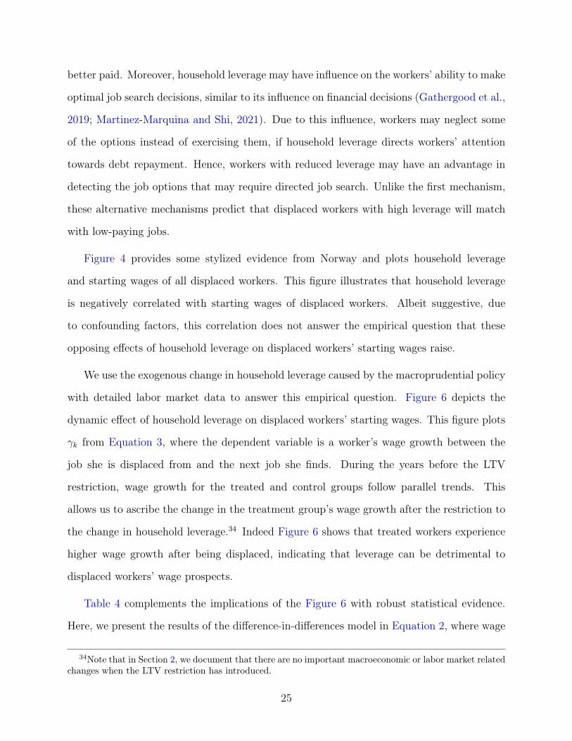
We use the exogenous change in household leverage caused by the macroprudential policy

with detailed labor market data to answer this empirical question. Figure 6 depicts the

dynamic effect of household leverage on displaced workers’ starting wages. This figure plots

γk from Equation 3, where the dependent variable is a worker’s wage growth between the

job she is displaced from and the next job she finds. During the years before the LTV

restriction, wage growth for the treated and control groups follow parallel trends. This

allows us to ascribe the change in the treatment group’s wage growth after the restriction to

the change in household leverage.34 Indeed Figure 6 shows that treated workers experience

higher wage growth after being displaced, indicating that leverage can be detrimental to

displaced workers’ wage prospects.

Table 4 complements the implications of the Figure 6 with robust statistical evidence.

Here, we present the results of the difference-in-differences model in Equation 2, where wage

34Note that in Section 2, we document that there are no important macroeconomic or labor market relatedchanges when the LTV restriction has introduced.

25

growth between job switches is the dependent variable. In Column (1), without any controls,

d(LTV > 0.85)h × Postt has a positive and statistically significant coefficient. In Column

(2), we include year fixed effects to control for time effects. A concern may be that treated

displaced workers have different education levels and that education can influence both labor

market outcomes and household leverage. If so, failing to control for education will create a

bias in the coefficient of interest. To mitigate this concern, we include education fixed effects

in Column (3). Another concern may be related to the construction of our sample. As

explained in Section 3.2, we restrict ourselves to workers who lost their jobs in mass layoffs.

Such layoffs could reasonably occur due to location or industry specific shocks. If these

shocks also affect labor market prospects, ignoring location and industry characteristics can

also generate a bias in our regressions. We therefore further saturate the model with location

and industry fixed effects in Columns (4) and (5).

Ideally, one would like to compare two workers who are displaced from the same firm.

However, in our sample, there are no firms with a mass layoff in both the pre- and post-

treatment period. As a consequence, d(LTV > 0.85)h × Postt would not be identified if we

were to include firm fixed effects. We therefore saturate the model with Location×Industry

fixed effects on Column (6). In this tight specification, d(LTV > 0.85)h × Postt has a

positive and statistically significant coefficient. The magnitude of the coefficient implies that

treated displaced workers experience a 45 percent higher wage growth rate after the policy

implementation. Since the mean wage growth rate for the treated workers is -7.4 percentage

points, the 45 percent higher growth implies that thanks to lower leverage, treated workers

achieve a relative gain in wages of 3.3 percentage points.

One concern about the causal interpretation of our results is endogenous selection. House-

holds that can buy a house before the policy may not be able to do so after the LTV restriction

due to the down payment that the restriction requires. Therefore, the treated households

before the restriction can be different than the treated households after the restriction in

terms of their ability to come up with enough savings for the down payment. If this is the

26

case, then the observed difference in the starting wages before and after the restriction can

be partially driven by the difference between the treated groups generated by the restriction.

This endogenous selection of the households is expected to be strongest around the pol-

icy implementation. After the announcement of the restriction, the households that think

that they cannot afford the down payment would try to purchase a house before the im-

plementation. Also, households with insufficient savings for the down payment but cannot

purchase before the implementation have to accumulate enough savings, which can delay

their purchase for some time. These two effects indicate that one way to tackle the selection

problem is excluding a time period right before and right after the policy from the sample.

As explained in Section 3, this is exactly what we do. By removing the six months before

the first LTV restriction implementation, we effectively exclude the households that can time

their purchase from the sample. Also, removing 18 months after the first implementation

gives an opportunity for the affected households to accumulate enough savings for the down

payment. Thanks to this "doughnut design", we expect to see that the endogenous selection

is minimal in our setting.

We document that this is indeed the case in two ways. First, we check whether the

LTV restriction alters the characteristics of the treated households in our sample.35 To this

end, we use log changes in income, wage, business income, transfers, unemployment benefits,

and education level one period before the layoff as the dependent variable for difference-in-

differences model in Equation 2. Confirming the effectiveness of our empirical design, the

restriction does not have statistically or economically significant effects on these characteris-

tics as shown in Table 5. In addition, incentives that property taxes create can be important

for this ineffectiveness. In Norway, households enjoy lower tax rates for their primary houses

when wealth tax is assessed.36 Therefore, due to the tax advantages, households have incen-

tives to increase the size of their real estate purchase as much as possible. This implies that

35Bernstein and Koudijs (2021) use a similar strategy for mortgage amortization policy in the Netherlands.36For primary houses, the tax value is 25 percent of the housing value with a tax rate of 0.7 percent.

27

when a restriction is introduced, the households still prefer purchasing a house but with a

lower price, which allows the characteristics of the home buyers stay the same.37 Moreover,

the first two columns of Table 5 mitigates another concern. One argument can be that

when workers observe that down payment requirements increase, they might start to look

for ways to increase their earnings. This may generate a momentum that can help them

in the job searching process once they are displaced. In this line of argument, our result

that low-leverage job seekers find better-paid jobs could partially reflect a momentum effect.

Finding that the restriction does not have an influence on previous income or wage growths

mitigates this concern effectively.

Second, we homogenize the treated households across the both periods in terms of their

ability to afford the down payment. As explained before, the main reason for the endogenous

selection is the changes in the treated households’ ability to afford the down payment. Thus,

refining the treated groups in terms of this ability mitigates the concerns regarding the

selection. First, we calculate the down payment for each home purchase using the policy

threshold. Then, we remove the households that do not have enough deposits for the down

payment from the pre-treatment period. Therefore, all households in this refined sample have

enough savings for the down payment. Table 6 documents that the estimated coefficients in

the refined sample are similar to the ones in Table 4, which indicates that our results does

not suffer from selection problems.

In Table 7, we provide several robustness checks for the impact of household leverage

on starting wages. First, to show that our results do not hinge on the sample period, we

change the sample starting period in the first two columns. Columns (1) and (2) reports the

results where we start the sample one year earlier or later. Doing so does not change our

results. Second, we remove all people who receive cash transfers greater than NOK 100,000

or have business income between 2000 and 2017, since their job search behavior may be

37We find that the LTV restriction decreases the house prices (Table A2).

28

different.38 Columns (3) and (4) document that removing such workers does not affect our

results. One concern might be that treated workers can react differently to macroeconomic

conditions. If a change in the macroeconomic conditions occurs around the time the LTV

restriction is implemented, the coefficient of d(LTV > 0.85)h × Postt could pick up this

differential response to these conditions. Although macroeconomic conditions were stable

(see Section 2), we take one step further in Column (5) and interact inflation, unemployment

rate, GDP growth, and the monetary policy rate with d(LTV > 0.85)h. Doing so increases

the positive impact of leverage on displaced workers’ wage growth. In Table A13, we show

that all interaction terms of d(LTV > 0.85)h with the four macro variables are insignificant,

indicating that wage growth for treated employees is not differentially affected by the macro

conditions. Finally, we saturate the model with d(LTV > 0.85)h×Education fixed effects to

verify if education affects the treated employees differently than the control group. Column

(6) shows that this does not change our results either.

The main selection criterion in the construction of the treated and control groups is the

cut-off value of the LTV ratio. Before the introduction of the policy, these two groups have

different LTV ratios. After adoption of the mortgage restriction, treated households have

lower LTV ratios than they would have chosen in an unconstrained market. This suggests

that treated households, in the post-treatment period, should be expected to have LTV ratios

just below the policy threshold. If true, then observations from the treatment and control

groups with LTVs just below the policy threshold would make a better comparison, since

they are more similar in terms of the main selection criterion. In our baseline regressions,

the lower bound for the LTV ratio is 50 percent. If this value is reasonable, then narrowing

the sample selection criteria from 50 percent towards to policy threshold (i.e. 85 percent)

should not affect the estimated treatment effect. We demonstrate that this is the case.

Figure 7 plots the coefficient of d(LTV > 0.85)h × Post from Equation 2, where we include

year, education, location, and industry fixed effects. The y-axis shows the coefficient of

38The cash transfers can be an inheritance or a gift by parents.

29

d(LTV > 0.85)h × Postt and the bars reflect the confidence 95 percent bands. Moving

rightward along the x-axis, each step raises the sample’s lower bound for the LTV ratio by 5

percent. Since the coefficient on d(LTV > 0.85)h × Postt remains virtually unchanged, we

can alleviate any concerns that observed wage growth differences between the treated and

control workers are a result of inherent differences due to the selection criterion.

Figure 6 clearly depicts that the treated and control groups have parallel trends in the out-

come variable before the treatment. However, fundamental differences between the treated

and control job seekers could be driving our results. We tackle this concern with a placebo

test. First, we remove the observations that occurred after the LTV ratio restriction. Then,

we create a dummy variable, Placebot that takes the value of one for the two periods before

the restriction and zero for the earlier periods. Moreover, we also remove the households

whose LTV ratios above the threshold from the placebo post sample. This helps us to

mimic exactly sample construction of the main sample.39 After these sample adjustments,

we interact Placebot with d(LTV > 0.85)h as if there exists a shock at the beginning of the

placebo period. If the results are driven by the differences between the treated and control

groups, d(LTV > 0.85)h × Placebot should have a significant coefficient. Table 8 shows

this is not the case. Analogous to Table 4, we run regressions without controls and then

add year, education, location, industry, and location×industry fixed effects consecutively.

In none of the models d(LTV > 0.85)h × Placebot has a significant and/or economically

sizeable coefficients, allaying any concerns about the parallel trends assumption.

5.3 Through what mechanism does leverage affect wages?

After establishing that displaced workers with low leverage have higher wage growth, we turn

to investigating through what mechanism leverage affects these workers’ starting salaries.

To better understand this, we start by inspecting job search behavior. First, we look at

39In Section A3 we use a simulation exercise and show that this removal does not create a bias in ourestimations.

30

the extent to which the time that displaced workers spend unemployed depends on their

leverage. Next, we investigate displaced workers’ debt utilization after the displacement.

Then, we analyze whether household leverage has an impact on employer and occupation

characteristics. Finally, we provide several heterogeneity tests that support the mechanism

that we reveal.

High leverage increases the probability of default. Following a negative income shock,

such as a job loss, workers with higher leverage may find it harder to avoid the default.

Hence, they may be willing to accept early job offers to avoid the default. To test this

hypothesis that leverage shortens the unemployment spells of high-leverage workers, we use

the employee-employer register and calculate the unemployment spells. Then, we enlist

the difference-in-differences model in Equation 2, now with the log of displaced workers’

unemployment spells, measured in days, as the dependent variable. First two columns of

Table 9 provides the results. Column (1) indicates that job seekers with lower leverage have

60 percent longer unemployment spells, an increase of 79 days. In Column (2), we saturate

the model with year, education, location, and industry fixed effects to control for time effects,

individual characteristics, and firms’ labor demand. These fixed effects do not change our

results qualitatively and in fact marginally increases the size of the measured effect.

One channel through which household leverage affects the job search behavior could be its

influence on debt usage during the unemployment spell. Literature has documented that ac-

cess to credit during the unemployment spell affects the job search behavior and labor market

outcomes (Herkenhoff et al., 2016; Herkenhoff, 2019). If leverage before the job displacement

affects the debt utilization during the unemployment spell, then this ex-post debt utilization

can be important for the findings we document. Our data set allows us to calculate the log

change in ex-post debt using the household balance sheet information. Columns (3) and (4)

of Table 9 use this variable as the dependent variable. These columns indicate that the LTV

ratio restriction does not affect the ex-post debt utilization as d(LTV > 0.85)h × Postt has

insignificant coefficients in both columns.

31

After documenting that household leverage before the displacement is important for

having longer unemployment spells, now we ask whether lower leverage helps displaced

workers find better employers? To address this question, we follow Abowd et al. (1999)

(AKM) and estimate the firm wage premium, i.e., the wages that firms pay after controlling

for employee characteristics, for all firms in our sample. To this end, we regress the log of

wages on employer, employee, and year fixed effects as well as employee characteristics.40

Then, we use the estimated firm fixed effects as firm wage premia. To understand whether

having lower leverage helps displaced workers find a better match, we take the difference

between wage premiums of new and old employers of workers, ∆Firm Wage Premium, and

use it as the dependent variable in our difference-in-differences setting. The last two columns

of Table 9 establish that treated workers experience a statistically significant increase in their

new employers’ wage premiums. Even though the effect is not significant without any fixed

effects, once we include year, education, location, and industry fixed effects, the coefficient

becomes highly statistically significant. The size of the coefficient in Column (6) implies that

about 20 percent of the increase in workers’ wage growth is driven by their finding jobs in

higher-paying firms.

A reduction in household leverage caused by the LTV restriction might alter the scope

of job search. To appreciate the impact that leverage has, we analyze three measures of

job search scope: occupation, industry, and location. Specifically, we use our difference-in-

differences model to test whether workers with low leverage are more likely to make a change

along any of these three dimensions. The results in Table 10 indicate that lower leverage

induces workers to broaden their job search along some margins. In Table 10, the odd-

numbered columns do not include any fixed effects and the even-numbered columns include

year, education, location, and industry fixed effects. In the first two columns, the dependent

variable is a dummy, which is 1 if a worker has a different occupation in her new firm. Switch-

ing to other occupations and/or industries can be helpful for displaced workers to reduce

40We remove the firms with fewer than 5 movers to reduce the labor mobility bias. In the AKM samplewe also discard job seekers from our estimation sample.

32

the scarring effect of job displacements (Ruhm, 1991; Stevens, 1997; Arulampalam, 2001).

Columns (1) and (2) show that displaced workers with lower leverage are 20 percent more

likely to take a different occupation when starting at their new employer. Columns (3) and

(4) demonstrate that lower leverage displaced workers also have a 15 percent higher probabil-

ity of finding their new jobs in other industries than before their displacement.Geographical

labor mobility, an important determinant of labor supply, has been shown to be adversely

affected when a household has negative home equity. We find that leverage, when isolated

from a household’s home equity position, does not affect displaced workers’ geographic labor

mobility. This complements the findings of Bernstein (2020) and Gopalan et al. (2020).

Together, our findings provide a clear picture of the mechanism through which a reduction

in leverage increases workers’ starting wages. Thanks to lower leverage, displaced workers

can afford to stay unemployed for longer duration. Also, they are able to find jobs in

firms with a higher wage premium. Moreover, they can broaden their job search reach by

switching to other occupations and/or other industries. Intuitively, we expect this mechanism

to be stronger and the observed effect on starting wages larger for job seekers who are in

a position to benefit more from improved matching. To verify this, we again run wage

growth regressions for displaced workers while splitting up our sample using three different

criteria. First, we assign households to either a lower or higher age half. Younger people

are expected to exploit the opportunity of a better job search more, since they can use

the longer spells to make investments to their skills and it is easier for them to switch

to other occupations and industries. The first two columns of Table 11 confirm that the

increase in wage growth is around 70 percent for workers younger than 33, substantially

higher than in the full sample. For the older job seekers the effect is insignificant. Next,

we split up job seekers by the duration of their tenure at their previous employer. Working

for the same firm for a long time may diminish a worker’s job search skills and lead to

the development of firm-specific human capital that is of limited value to new employers.

For such workers, it may be challenging to exploit the opportunity of a better job search.

33

Columns (3) and (4) support this intuition. The effect of having low leverage is stronger

for workers with a below median tenure. Finally, we break down our sample into workers

whose highest educational attainment is upper secondary school or lower, and those who

have an undergraduate degree. Higher education can facilitate the process of switching to

other occupations and industries. Moreover, Eriksson and Rooth (2014) have documented for

Sweden that longer unemployment spells diminish employers’ return rates to job applications

for medium and low skill jobs, suggestive of a negative correlation between unemployment

spells and starting wages for workers with low education. In line with Eriksson and Rooth

(2014) and our intuition, we report that the rise in wage growth is larger for higher educated

workers.

Discussions about LTV restriction policies point out that they affect the households

with lower income more strongly, since affording the down payment is more demanding for

such households (Van Bekkum et al., 2019). Due to the down payments that the LTV

restrictions introduce, low-income households can change their consumption patterns, which

may not be optimal from a welfare point of view. However, for workers from low-income

households, a reduction in leverage can generate higher improvements in their starting wages

since a reduction in deb-related payments creates a relatively larger cash release. To this

end, we divide our sample into three groups with respect to the income levels. The first

three columns of Table 12 document that the improvement in starting wages is significantly

stronger for workers from low-income households. This finding indicates that even though

an LTV ratio restriction can affect the low-income household negatively during the home-

purchasing process, it allows them to improve their wages.

One robust finding on wages is that female workers earn less than their male counter-

parts. In addition to the other factors, differences in risk-aversion or in salary demands

can contribute to the gender pay gap (Blau and Kahn, 2017; Roussille, 2020; Cortés et al.,

2021). These findings imply that the impact of a reduction in leverage on starting wages

can be affected by the worker’s gender. For instance, a worker with higher risk-aversion can

34

reduce her job search duration by accepting an earlier job offer, even though she may receive

an offer with a higher salary if she was on the labor market. Or, due to higher leverage a

worker can reduce her ask salary to increase the chances of getting a job offer. To test how

worker’s gender differentiates the impact of a reduction in leverage on starting wages, we

split our sample into two with respect to worker’s gender. The last two columns of Table 12

clearly show that the positive effect of the reduction in leverage on starting wages is stronger

for female workers, which complements the findings of (Roussille, 2020; Cortés et al., 2021).

Overall, our results suggest that a reduction in leverage particularly improves the starting

wages of disadvantaged workers.

5.4 Longer-term effects

The effect of leverage on starting wages that we identified in section 5.2 could be temporary.

If previously displaced workers whose starting wage is lower continue to search for better

paying jobs after accepting an initial job offer, then the effect of leverage on wages would

be attenuated over time. If however, search intensity falls after job acceptance, or when

human capital quickly becomes firm-specific, the effect could be long-lasting. To document

the persistence of the effect we estimate, we track workers’ annual wages for four years after

their displacement. Then, we calculate the growth rates of wages during these four years

and use this variable as the dependent variable in the difference-in-differences model. We

report the results in Table 13. The policy-induced reduction in leverage raises the four-year

wage growth by 28 percent. This number indicates a 4.7 percentage points improvement

in the annual wages during this 4-year period. The magnitude of the effect is robust to

saturating the model with year, education, location, industry, and location×industry fixed

effects. Together, these findings establish that the increase in wage growth is robust and not

short-lived.

Finally, we consider the treated workers’ wage volatility. Section 5.3 established that

35

lower leverage facilitated employees switching to other occupations and industries. Shifting

to other occupations and/or other industries may increase wage volatility, for example due

to a lack of appropriate experience in these new occupations or industries. If, however,

matching quality improves thanks to lower leverage, then we would expect to observe that

lower-leverage job seekers have lower wage volatility after the LTV restriction. To test how

the wage volatility is affected by the reduction in leverage, we calculate the standard deviation

of annual wages for four years post-displacement and use it as the dependent variable in

Equation 2. Table 14 makes clear that lower-leverage households have significantly lower

wage volatility. In addition to the increase in wage growth, lower leverage thus further

improves labor market outcomes by making the wages more stable. One interpretation of

this finding can be that thanks to the lower leverage, workers have a better match in the

labor market, which reduces their wage volatility.

6 Discussion

Household leverage is an extensively studied driver of the economy. Spurred by the effects

of the 2008-2009 financial crisis, academics and policymakers have since attempted to design

and evaluate policies to mitigate the undesirable consequences of household leverage for the

economy. Labor market outcomes and job search are both key variables for the economy as

well. Empirical evidence on the relationship between households’ leverage and Labor market

outcomes and job search is limited, however.

Difficulties in obtaining high-quality register data and the fact that decisions on jobs and

debt are taken simultaneously are explanations for our incomplete understanding of the in-

terrelationship between labor market outcomes and debt. Our research strategy attempts to

overcome these challenges and make an advance in the identification of household leverage’s

importance for labor market outcomes. We exploit the introduction of a macroprudential

policy in Norway that exogenously reduces households’ leverage through a maximum LTV

36

ratio restriction for home purchases. Using data for the entire adult population of Norway

and information on mass layoffs, the policy change permits us to causally identify the impact

of household leverage on labor market outcomes.

Our work is closely related to the literature that studies the determinants of labor supply

and job search. We show that limiting household leverage generates persistent and positive

effects on displaced workers’ wages. We make several specific contributions. First, we confirm

that an LTV ratio restriction is highly effective in constraining borrowing by households.

Second, we causally identify the effect of leverage on starting wages of displaced workers and

find that displaced workers have a 3.3 percentage points higher wage following a 25 percent

decline in their debt-to-income ratio. Third, displaced workers, following a reduction in debt

engage in a longer job search and find jobs at firms that pay higher wages, switches into new

occupations and different industry also become more likely. We argue this is made possible

when lower debt service reduces the pressure on displaced workers to quickly accept job

offers. Firm-specific wage premia explain 20 percent of the gain in starting wages. Moreover,

younger, more highly educated workers with shorter job tenure experience stronger effects

on their wages. Finally, the identified effects are not short-lived and rather appear to be

reinforced over time.

Our results also relate to studies of the effects of credit access and household leverage

on the economy, and inform the debate on the effectiveness of macroprudential policies.

Research has mainly focused on the effectiveness of macroprudential policies in restraining

credit and housing markets. These policies are often most binding for young households

without equity and can lead to postponement of households’ home purchasing (Fuster and

Zafar, 2016; Van Bekkum et al., 2019) or reductions in housing market access (Tzur-Ilan,

2020). Our results indicate that macroprudential policies also bring about economically

significant and sustained benefits for low income, highly indebted, young, and female workers.

This suggests that policymakers should internalize a broader range of beneficial effects when

designing macroprudential policies.

37

The findings in this paper potentially have bearing on other policy choices that affect

what leverage levels are efficient in an economy. When household leverage influences the

career and income path of workers, policies to alter debt may have knock-on effects on

wealth, health, family conditions, offspring or even political choice. The existence and size of

such downstream effects would in turn affect the social value of household leverage-reducing

policies.

38

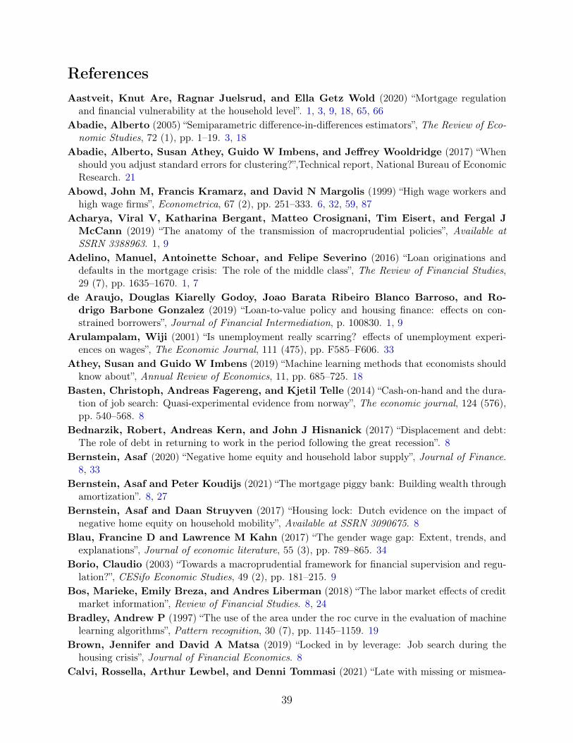
ReferencesAastveit, Knut Are, Ragnar Juelsrud, and Ella Getz Wold (2020) “Mortgage regulation

and financial vulnerability at the household level”. 1, 3, 9, 18, 65, 66Abadie, Alberto (2005) “Semiparametric difference-in-differences estimators”, The Review of Eco-

nomic Studies, 72 (1), pp. 1–19. 3, 18Abadie, Alberto, Susan Athey, Guido W Imbens, and Jeffrey Wooldridge (2017) “When

should you adjust standard errors for clustering?”,Technical report, National Bureau of EconomicResearch. 21

Abowd, John M, Francis Kramarz, and David N Margolis (1999) “High wage workers andhigh wage firms”, Econometrica, 67 (2), pp. 251–333. 6, 32, 59, 87

Acharya, Viral V, Katharina Bergant, Matteo Crosignani, Tim Eisert, and Fergal JMcCann (2019) “The anatomy of the transmission of macroprudential policies”, Available atSSRN 3388963. 1, 9

Adelino, Manuel, Antoinette Schoar, and Felipe Severino (2016) “Loan originations anddefaults in the mortgage crisis: The role of the middle class”, The Review of Financial Studies,29 (7), pp. 1635–1670. 1, 7

de Araujo, Douglas Kiarelly Godoy, Joao Barata Ribeiro Blanco Barroso, and Ro-drigo Barbone Gonzalez (2019) “Loan-to-value policy and housing finance: effects on con-strained borrowers”, Journal of Financial Intermediation, p. 100830. 1, 9

Arulampalam, Wiji (2001) “Is unemployment really scarring? effects of unemployment experi-ences on wages”, The Economic Journal, 111 (475), pp. F585–F606. 33

Athey, Susan and Guido W Imbens (2019) “Machine learning methods that economists shouldknow about”, Annual Review of Economics, 11, pp. 685–725. 18

Basten, Christoph, Andreas Fagereng, and Kjetil Telle (2014) “Cash-on-hand and the dura-tion of job search: Quasi-experimental evidence from norway”, The economic journal, 124 (576),pp. 540–568. 8

Bednarzik, Robert, Andreas Kern, and John J Hisnanick (2017) “Displacement and debt:The role of debt in returning to work in the period following the great recession”. 8

Bernstein, Asaf (2020) “Negative home equity and household labor supply”, Journal of Finance.8, 33

Bernstein, Asaf and Peter Koudijs (2021) “The mortgage piggy bank: Building wealth throughamortization”. 8, 27

Bernstein, Asaf and Daan Struyven (2017) “Housing lock: Dutch evidence on the impact ofnegative home equity on household mobility”, Available at SSRN 3090675. 8

Blau, Francine D and Lawrence M Kahn (2017) “The gender wage gap: Extent, trends, andexplanations”, Journal of economic literature, 55 (3), pp. 789–865. 34

Borio, Claudio (2003) “Towards a macroprudential framework for financial supervision and regu-lation?”, CESifo Economic Studies, 49 (2), pp. 181–215. 9

Bos, Marieke, Emily Breza, and Andres Liberman (2018) “The labor market effects of creditmarket information”, Review of Financial Studies. 8, 24

Bradley, Andrew P (1997) “The use of the area under the roc curve in the evaluation of machinelearning algorithms”, Pattern recognition, 30 (7), pp. 1145–1159. 19

Brown, Jennifer and David A Matsa (2019) “Locked in by leverage: Job search during thehousing crisis”, Journal of Financial Economics. 8

Calvi, Rossella, Arthur Lewbel, and Denni Tommasi (2021) “Late with missing or mismea-

39

sured treatment”. 18Card, David, Raj Chetty, and Andrea Weber (2007) “Cash-on-hand and competing mod-

els of intertemporal behavior: New evidence from the labor market”, The Quarterly journal ofeconomics, 122 (4), pp. 1511–1560. 8

Cerutti, Eugenio, Stijn Claessens, and Luc Laeven (2017) “The use and effectiveness ofmacroprudential policies: New evidence”, Journal of Financial Stability, 28, pp. 203–224. 9

Cesarini, David, Erik Lindqvist, Matthew J Notowidigdo, and Robert Östling (2017)“The effect of wealth on individual and household labor supply: evidence from swedish lotteries”,American Economic Review, 107 (12), pp. 3917–46. 8

Cespedes, Jacelly, Zack Liu, and Carlos Parra (2020) “Almost famous: How wealth shocksimpact career choices”, Available at SSRN 3491426. 8

Charles, Kerwin Kofi and Melvin Stephens, Jr (2004) “Job displacement, disability, anddivorce”, Journal of Labor Economics, 22 (2), pp. 489–522. 9

Chetty, Raj (2008) “Moral hazard versus liquidity and optimal unemployment insurance”, Journalof political Economy, 116 (2), pp. 173–234. 8

Chetty, Raj and Adam Szeidl (2007) “Consumption commitments and risk preferences”, TheQuarterly Journal of Economics, 122 (2), pp. 831–877. 2, 24

Claessens, Stijn (2015) “An overview of macroprudential policy tools”. 1Claessens, Stijn, Swati R Ghosh, and Roxana Mihet (2013) “Macro-prudential policies to

mitigate financial system vulnerabilities”, Journal of International Money and Finance, 39, pp.153–185. 9

Corbae, Dean and Erwan Quintin (2015) “Leverage and the foreclosure crisis”, Journal ofPolitical Economy, 123 (1), pp. 1–65. 7

Cortés, Patricia, Jessica Pan, Laura Pilossoph, and Basit Zafar (2021) “Gender differencesin job search and the earnings gap: Evidence from business majors”,Technical report, NationalBureau of Economic Research. 34, 35

Couch, Kenneth A and DanaW Placzek (2010) “Earnings losses of displaced workers revisited”,American Economic Review, 100 (1), pp. 572–89. 9

Dávila, Eduardo and Anton Korinek (2018) “Pecuniary externalities in economies with financialfrictions”, The Review of Economic Studies, 85 (1), pp. 352–395. 9

Davis, Steven J, John C Haltiwanger, Scott Schuh et al. (1998) “Job creation and destruc-tion”, MIT Press Books, 1. 16

Davis, Steven J and Till M Von Wachter (2011) “Recessions and the cost of job loss”,Technicalreport, National Bureau of Economic Research. 9

Defusco, Anthony A, Stephanie Johnson, and John Mondragon (2019) “Regulating House-hold Leverage”, The Review of Economic Studies, rdz040. 9

Diamond, Rebecca, Adam Guren, and Rose Tan (2020) “The effect of foreclosures on home-owners, tenants, and landlords”,Technical report, National Bureau of Economic Research. 24

Dobbie, Will, Paul Goldsmith-Pinkham, Neale Mahoney, and Jae Song (2020) “Badcredit, no problem? credit and labor market consequences of bad credit reports”, The Journal ofFinance, 75 (5), pp. 2377–2419. 24

Dobbie, Will and Jae Song (2015) “Debt relief and debtor outcomes: Measuring the effects ofconsumer bankruptcy protection”, American Economic Review, 105 (3), pp. 1272–1311. 24

Donaldson, Jason Roderick, Giorgia Piacentino, and Anjan Thakor (2019) “Householddebt overhang and unemployment”, The Journal of Finance, 74 (3), pp. 1473–1502. 1, 24

40

Eggertsson, Gauti B and Paul Krugman (2012) “Debt, deleveraging, and the liquidity trap:A fisher-minsky-koo approach”, The Quarterly Journal of Economics, 127 (3), pp. 1469–1513. 7

Elul, Ronel, Nicholas S Souleles, Souphala Chomsisengphet, Dennis Glennon, andRobert Hunt (2010) “What" triggers" mortgage default?”, American Economic Review, 100(2), pp. 490–94. 66

Eriksson, Stefan and Dan-Olof Rooth (2014) “Do employers use unemployment as a sortingcriterion when hiring? evidence from a field experiment”, American economic review, 104 (3), pp.1014–39. 34

Farhi, Emmanuel and Iván Werning (2016) “A theory of macroprudential policies in the pres-ence of nominal rigidities”, Econometrica, 84 (5), pp. 1645–1704. 1, 9

Favilukis, Jack, Sydney C Ludvigson, and Stijn Van Nieuwerburgh (2017) “The macroeco-nomic effects of housing wealth, housing finance, and limited risk sharing in general equilibrium”,Journal of Political Economy, 125 (1), pp. 140–223. 1

Finanstilsynet (2011) “Finanstilsynet considers tightening the guidelines for prudent residentialmortgage lending practice”, Press Release, 38. 11, 17

Flaaen, Aaron, Matthew D Shapiro, and Isaac Sorkin (2019) “Reconsidering the conse-quences of worker displacements: Firm versus worker perspective”, American Economic Journal:Macroeconomics, 11 (2), pp. 193–227. 14

Fontaine, François, Janne Nyborg Jensen, and Rune Majlund Vejlin (2020) “Wealth,portfolios, and unemployment duration”. 8

Fuster, Andreas and Paul S Willen (2017) “Payment size, negative equity, and mortgagedefault”, American Economic Journal: Economic Policy, 9 (4), pp. 167–91. 66

Fuster, Andreas and Basit Zafar (2016) “To buy or not to buy: Consumer constraints in thehousing market”, American Economic Review, 106 (5), pp. 636–40. 37

Galati, Gabriele and Richhild Moessner (2013) “Macroprudential policy–a literature review”,Journal of Economic Surveys, 27 (5), pp. 846–878. 1

Ganong, Peter and Pascal J Noel (2020) “Why do borrowers default on mortgages? a newmethod for causal attribution”,Technical report, National Bureau of Economic Research. 66

Gathergood, John, Neale Mahoney, Neil Stewart, and Jörg Weber (2019) “How do indi-viduals repay their debt? the balance-matching heuristic”, American Economic Review, 109 (3),pp. 844–75. 25

Gopalan, Radhakrishnan, Barton H Hamilton, Ankit Kalda, and David Sovich (2020)“Home equity and labor income: The role of constrained mobility”, The Review of FinancialStudies. 8, 33

Gross, Tal, Matthew J Notowidigdo, and Jialan Wang (2020) “The marginal propensityto consume over the business cycle”, American Economic Journal: Macroeconomics, 12 (2), pp.351–84. 24

Guerrieri, Veronica and Guido Lorenzoni (2017) “Credit crises, precautionary savings, andthe liquidity trap”, The Quarterly Journal of Economics, 132 (3), pp. 1427–1467. 7

Gupta, Arpit and Christopher Hansman (2020) “Selection, leverage, and default in the mort-gage market”, Available at SSRN 3315896. 66

Halla, Martin, Julia Schmieder, and Andrea Weber (2020) “Job displacement, family dy-namics, and spousal labor supply”, American Economic Journal: Applied Economics, 12 (4), pp.253–87. 9

He, Alex Xi and Daniel le Maire (2020) “How does liquidity constraint affect employment and

41

wages? evidence from danish mortgage reform”. 8, 18Herkenhoff, Kyle F (2019) “The impact of consumer credit access on unemployment”, The Review

of Economic Studies, 86 (6), pp. 2605–2642. 8, 31Herkenhoff, Kyle, Gordon Phillips, and Ethan Cohen-Cole (2016) “How credit constraints

impact job finding rates, sorting & aggregate output”,Technical report, National Bureau of Eco-nomic Research. 31

Hosmer Jr, David W, Stanley Lemeshow, and Rodney X Sturdivant (2013) Applied logisticregression, 398, John Wiley & Sons. 19

Ichino, Andrea, Guido Schwerdt, Rudolf Winter-Ebmer, and Josef Zweimüller (2017)“Too old to work, too young to retire?”, The Journal of the Economics of Ageing, 9, pp. 14–29. 9

Igan, Deniz and Heedon Kang (2011) “Do loan-to-value and debt-to-income limits work? evi-dence from korea”, IMF Working Papers, pp. 1–34. 9

Jacobson, Louis S, Robert J LaLonde, and Daniel G Sullivan (1993) “Earnings losses ofdisplaced workers”, The American Economic Review, pp. 685–709. 9

James, Gareth, Daniela Witten, Trevor Hastie, and Robert Tibshirani (2013) An intro-duction to statistical learning, 112, Springer. 19

Ji, Yan (2021) “Job search under debt: Aggregate implications of student loans”, Journal of Mon-etary Economics, 117, pp. 741–759. 2, 24

Kumar, Anil and Che-Yuan Liang (2018) “Labor market effects of credit constraints: Evidencefrom a natural experiment”. 8

Lachowska, Marta, Alexandre Mas, and Stephen A. Woodbury (2020) “Sources of displacedworkers’ long-term earnings losses”, American Economic Review, 110 (10), pp. 3231–66. 9, 14

Lalive, Rafael, Jan Van Ours, and Josef Zweimüller (2006) “How changes in financial in-centives affect the duration of unemployment”, The Review of Economic Studies, 73 (4), pp.1009–1038. 8

Lewbel, Arthur (2007) “Estimation of average treatment effects with misclassification”, Econo-metrica, 75 (2), pp. 537–551. 21

Li, Han, Jiangyi Li, Yi Lu, and Huihua Xie (2020) “Housing wealth and labor supply: Evidencefrom a regression discontinuity design”, Journal of Public Economics, 183, p. 104139. 8

Maggio, Marco Di, Ankit Kalda, and Vincent Yao (2019) “Second chance: Life withoutstudent debt”,Technical report, National Bureau of Economic Research. 24

Martinez-Marquina, Alejandro and Mike Shi (2021) “The burden of household debt”. 25Meekes, Jordy and Wolter HJ Hassink (2019) “Endogenous local labour markets, regional

aggregation and agglomeration economies”. 8Mian, Atif, Kamalesh Rao, and Amir Sufi (2013) “Household balance sheets, consumption,

and the economic slump”, The Quarterly Journal of Economics, 128 (4), pp. 1687–1726. 7Mian, Atif and Amir Sufi (2011) “House prices, home equity-based borrowing, and the us

household leverage crisis”, American Economic Review, 101 (5), pp. 2132–56. 1Mian, Atif and Amir Sufi (2014) “What explains the 2007–2009 drop in employment?”, Econo-

metrica, 82 (6), pp. 2197–2223. 7Mian, Atif, Amir Sufi, and Emil Verner (2017) “Household debt and business cycles worldwide”,

The Quarterly Journal of Economics, 132 (4), pp. 1755–1817. 1, 7Ministry of Finance (2021) “The mortgage regulations 1 january 2020–31. december 2020”. 11Moore, Brendan and Judith Scott-Clayton (2019) “The firm’s role in displaced workers’ earn-

ings losses”,Technical report, National Bureau of Economic Research. 9

42

Mulligan, Casey B (2009) “Means-tested mortgage modification: Homes saved or income de-stroyed?”,Technical report, National Bureau of Economic Research. 8

Mulligan, Casey B (2010) “Foreclosures, enforcement, and collections under the federal mortgagemodification guidelines”,Technical report, National Bureau of Economic Research. 8

Murphy, Kevin M and Robert H Topel (1985) “Estimation and inference in two-step econo-metric models”, Journal of Business & Economic Statistics, 3 (4), pp. 88–97. 21

Peydró, José-Luis, Francesc Rodriguez Tous, Jagdish Tripathy, and Arzu Uluc (2020)“Macroprudential policy, mortgage cycles and distributional effects: Evidence from the uk”. 1, 9

Pizzinelli, Carlo (2018) “Housing, borrowing constraints, and labor supply over the life cy-cle”,Technical report, Working paper. 9

Reinhart, Carmen M and Kenneth S Rogoff (2008) “This time is different: A panoramic viewof eight centuries of financial crises”,Technical report, National Bureau of Economic Research. 1,7

Rothstein, Jesse (2011) “Unemployment insurance and job search in the great recession”,Technicalreport, National Bureau of Economic Research. 8

Rothstein, Jesse and Cecilia Elena Rouse (2011) “Constrained after college: Student loansand early-career occupational choices”, Journal of Public Economics, 95 (1), pp. 149–163. 8

Roussille, Nina (2020) “The central role of the ask gap in gender pay inequality”, URL:https://ninaroussille. github. io/files/Roussille_ askgap. pdf. 34, 35

Ruhm, Christopher J (1991) “Are workers permanently scarred by job displacements?”, TheAmerican economic review, 81 (1), pp. 319–324. 33

Schmieder, J, Till von Wachter, and Jörg Heining (2018) “The costs of job displacement overthe business cycle and its sources: evidence from germany”,Technical report, UCLA, Mimeo. 9

Schularick, Moritz and Alan M Taylor (2012) “Credit booms gone bust: Monetary policy,leverage cycles, and financial crises, 1870-2008”, American Economic Review, 102 (2), pp. 1029–61. 1, 7

Statistics Norway (1998) “Standard classification of occupations”. 16Stevens, Ann Huff (1997) “Persistent effects of job displacement: The importance of multiple job

losses”, Journal of Labor Economics, 15 (1, Part 1), pp. 165–188. 33Sullivan, Daniel and Till Von Wachter (2009) “Job displacement and mortality: an analysis

using administrative data”, The Quarterly Journal of Economics, 124 (3), pp. 1265–1306. 14Sullivan, Daniel and Till von Wachter (2009) “Job Displacement and Mortality: An Analysis

Using Administrative Data*”, The Quarterly Journal of Economics, 124 (3), pp. 1265–1306. 9Tzur-Ilan, Nitzan (2020) “The real consequences of ltv limits on housing choices”,Technical report,

mimeo. 1, 9, 37, 66Van Bekkum, Sjoerd, Rustom M Irani, Marc Gabarro, and José Luis Peydró (2019)

“Macroprudential policy and household leverage: evidence from administrative household-leveldata”. 1, 3, 9, 18, 34, 37, 65, 66

Von Wachter, Till, Jae Song, and Joyce Manchester (2009) “Long-term earnings losses dueto mass layoffs during the 1982 recession: An analysis using us administrative data from 1974 to2004”, unpublished paper, Columbia University. 14

Zator, Michal (2019) “Working more to pay the mortgage: Household debt, consumption com-mitments and labor supply”. 8

43

Figure 1: Household debt and house prices

This figure shows the house price index (Figure 1a) and household credit to GDP ratio (Figure 1b) in Norway between 2000and 2019. The orange line indicates the implementation date of LTV ratio restriction.

(a)

5070

9011

013

015

017

0

2000 2002 2004 2006 2008 2010 2012 2014 2016 2018 2020Year

House Price Index

(b)

5060

7080

9010

0%

2000 2002 2004 2006 2008 2010 2012 2014 2016 2018 2020Year

Household Credit to GDP

44

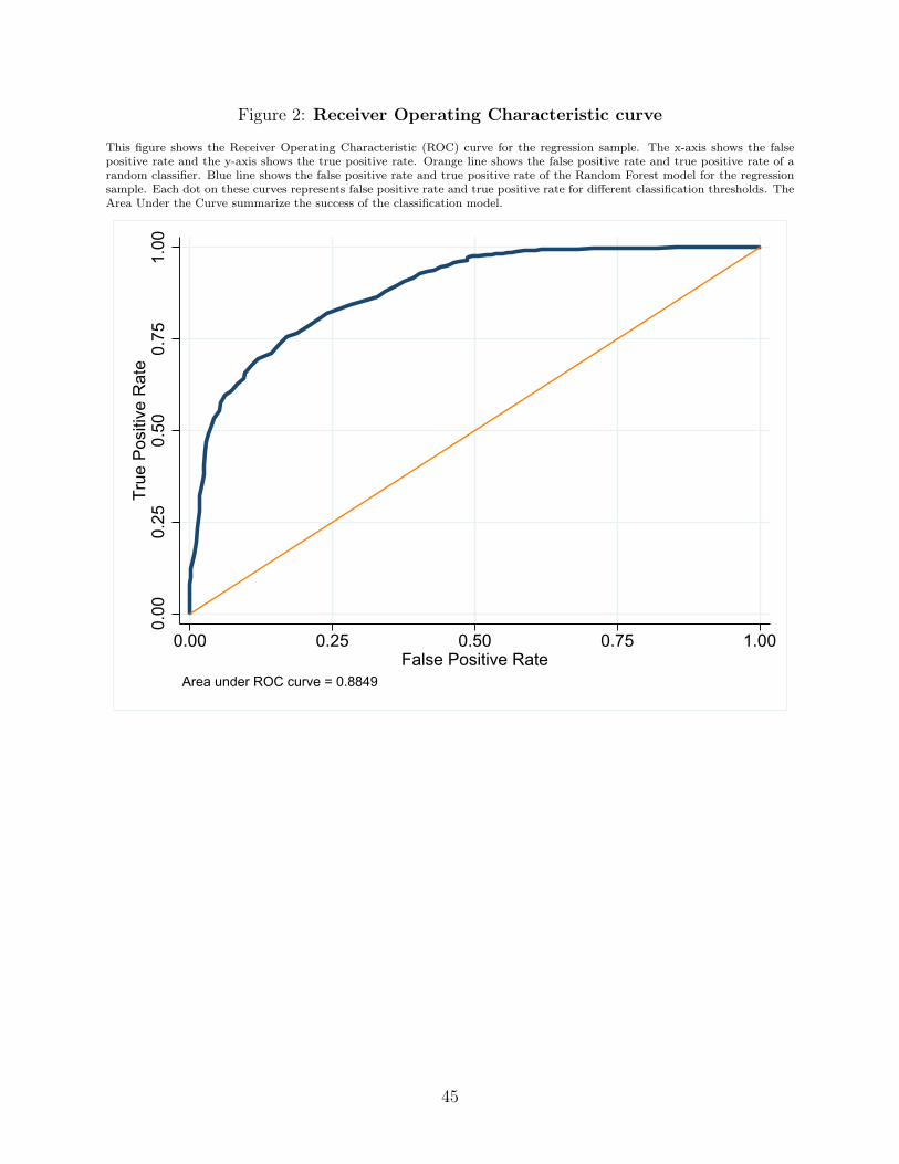
Figure 2: Receiver Operating Characteristic curve

This figure shows the Receiver Operating Characteristic (ROC) curve for the regression sample. The x-axis shows the falsepositive rate and the y-axis shows the true positive rate. Orange line shows the false positive rate and true positive rate of arandom classifier. Blue line shows the false positive rate and true positive rate of the Random Forest model for the regressionsample. Each dot on these curves represents false positive rate and true positive rate for different classification thresholds. TheArea Under the Curve summarize the success of the classification model.

0.00

0.25

0.50

0.75

1.00

True

Pos

itive

Rat

e

0.00 0.25 0.50 0.75 1.00False Positive Rate

Area under ROC curve = 0.8849

45

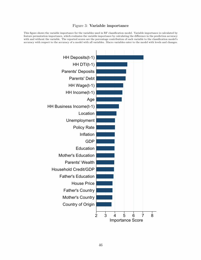
Figure 3: Variable importance

This figure shows the variable importance for the variables used in RF classification model. Variable importance is calculated byfeature permutation importance, which evaluates the variable importance by calculating the difference in the prediction accuracywith and without the variable. The reported scores are the percentage contribution of each variable to the classification model’saccuracy with respect to the accuracy of a model with all variables. Macro variables enter to the model with levels and changes.

2 3 4 5 6 7 8Importance Score

Country of OriginMother's CountryFather's Country

House PriceFather's Education

Household Credit/GDPParents' Wealth

Mother's EducationEducation

GDPInflation

Policy RateUnemployment

LocationHH Business Income(t-1)

AgeHH Income(t-1)

HH Wage(t-1)Parents' Debt

Parents' DepositsHH DTI(t-1)

HH Deposits(t-1)

46

Figure 4: Household debt and labor market outcomes

This figure shows that debt-to-income (DTI) ratio is negatively correlated with starting wages of displaced workers. The sampleconsists of workers who lost their jobs due to mass layoffs.

6.7

6.75

6.8

6.85

ln(S

tarti

ng W

age)

0 2 4 6 8Debt-to-Income

47

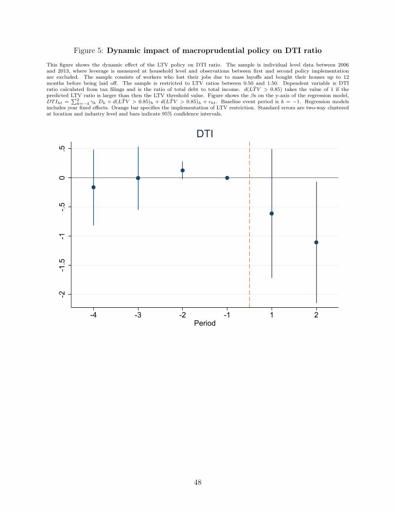
Figure 5: Dynamic impact of macroprudential policy on DTI ratio

This figure shows the dynamic effect of the LTV policy on DTI ratio. The sample is individual level data between 2006and 2013, where leverage is measured at household level and observations between first and second policy implementationare excluded. The sample consists of workers who lost their jobs due to mass layoffs and bought their houses up to 12months before being laid off. The sample is restricted to LTV ratios between 0.50 and 1.50. Dependent variable is DTIratio calculated from tax filings and is the ratio of total debt to total income. d( ˆLTV > 0.85) takes the value of 1 if thepredicted LTV ratio is larger than then the LTV threshold value. Figure shows the βs on the y-axis of the regression model,DTIht =

∑2k=−4 γk Dk × d( ˆLTV > 0.85)h + d( ˆLTV > 0.85)h + εht. Baseline event period is k = −1. Regression models

includes year fixed effects. Orange bar specifies the implementation of LTV restriction. Standard errors are two-way clusteredat location and industry level and bars indicate 95% confidence intervals.

-2-1

.5-1

-.50

.5

-4 -3 -2 -1 1 2Period

DTI

48

Figure 6: Dynamic impact of policy on wage growth

This figure shows the dynamic effect of the LTV policy on wage growth for displaced workers. The sample is individual leveldata between 2006 and 2013, where leverage is measured at household level and observations between first and second policyimplementation are excluded. The sample consists of workers who lost their jobs due to mass layoffs and bought their housesup to 12 months before being laid off. The sample is restricted to LTV ratios between 0.50 and 1.50. Dependent variable iswage growth between the wage in the previous job and the wage in the new job. d( ˆLTV > 0.85) takes the value of 1 if thepredicted LTV ratio is larger than then the LTV threshold value. Figure shows the βs on the y-axis of the regression modelwage growthht =

∑2k=−4 γk Dk × d( ˆLTV > 0.85)h + d( ˆLTV > 0.85)h + εht. Baseline event period is k = −1. Regression

models includes year fixed effects. Orange bar specifies the implementation of LTV restriction. Standard errors are two-wayclustered at location and industry level and bars indicate 95% confidence intervals.

-.50

.51

-4 -3 -2 -1 1 2Period

Wage Growth

49

Figure 7: Different thresholds for the LTV lower bound

This figure provides a robustness check for the effect of LTV policy on wage growth for displaced workers. The sample isindividual level data between 2006 and 2013, where leverage is measured at household level and observations between first andsecond policy implementation are excluded. The sample consists of workers who lost their jobs due to mass layoffs and boughttheir houses up to 12 months before being laid off. Dependent variable is wage growth between the wage in the previous joband the wage in the new job. d( ˆLTV > 0.85) takes the value of 1 if the predicted LTV ratio is larger than then the LTVthreshold value. Post equals to 1 for the years 2012 and 2013 and equals to 0 for earlier years. x-axis indicates the value of thelower bound for the LTV ratio to be included in the estimation sample. y-axis shows β from the Equation 2. Regression modelsinclude year, education, location, and industry fixed effects. Standard errors are two-way clustered at location and industrylevel and bars indicate 95% confidence intervals.

0.2

.4.6

.81

d(LT

V>0.

85) x

Pos

t

LTV>.55 LTV>.6 LTV>.65 LTV>.70 LTV>.75 LTV>.8LTV Thresholds

Different LTV Thresholds

50

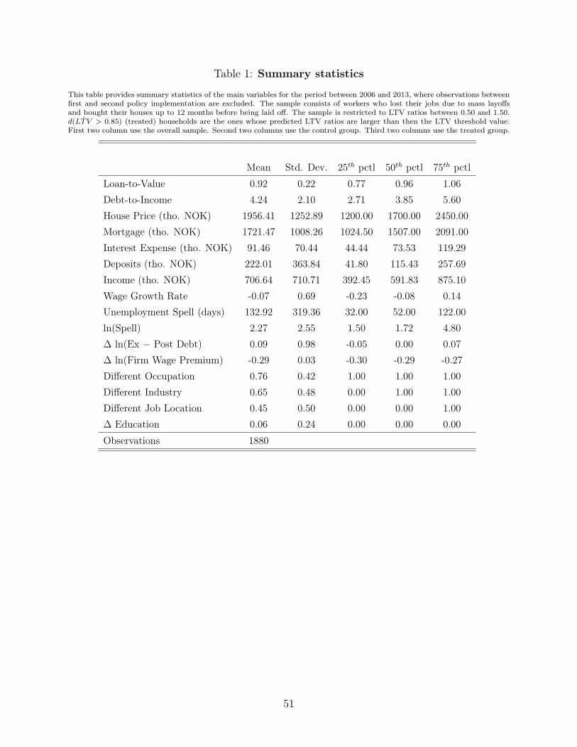
Table 1: Summary statistics

This table provides summary statistics of the main variables for the period between 2006 and 2013, where observations betweenfirst and second policy implementation are excluded. The sample consists of workers who lost their jobs due to mass layoffsand bought their houses up to 12 months before being laid off. The sample is restricted to LTV ratios between 0.50 and 1.50.d( ˆLTV > 0.85) (treated) households are the ones whose predicted LTV ratios are larger than then the LTV threshold value.First two column use the overall sample. Second two columns use the control group. Third two columns use the treated group.

Mean Std. Dev. 25th pctl 50th pctl 75th pctl

Loan-to-Value 0.92 0.22 0.77 0.96 1.06Debt-to-Income 4.24 2.10 2.71 3.85 5.60House Price (tho. NOK) 1956.41 1252.89 1200.00 1700.00 2450.00Mortgage (tho. NOK) 1721.47 1008.26 1024.50 1507.00 2091.00Interest Expense (tho. NOK) 91.46 70.44 44.44 73.53 119.29Deposits (tho. NOK) 222.01 363.84 41.80 115.43 257.69Income (tho. NOK) 706.64 710.71 392.45 591.83 875.10Wage Growth Rate -0.07 0.69 -0.23 -0.08 0.14Unemployment Spell (days) 132.92 319.36 32.00 52.00 122.00ln(Spell) 2.27 2.55 1.50 1.72 4.80∆ ln(Ex − Post Debt) 0.09 0.98 -0.05 0.00 0.07∆ ln(Firm Wage Premium) -0.29 0.03 -0.30 -0.29 -0.27Different Occupation 0.76 0.42 1.00 1.00 1.00Different Industry 0.65 0.48 0.00 1.00 1.00Different Job Location 0.45 0.50 0.00 0.00 1.00∆ Education 0.06 0.24 0.00 0.00 0.00

Observations 1880

51

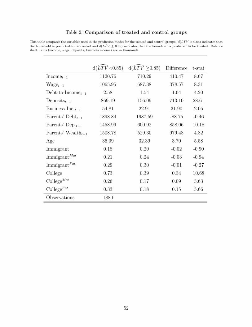
Table 2: Comparison of treated and control groups

This table compares the variables used in the prediction model for the treated and control groups. d( ˆLTV < 0.85) indicates thatthe household is predicted to be control and d( ˆLTV ≥ 0.85) indicates that the household is predicted to be treated. Balancesheet items (income, wage, deposits, business income) are in thousands.

d(LTV<0.85) d(LTV ≥0.85) Difference t-stat

Incomet−1 1120.76 710.29 410.47 8.67Waget−1 1065.95 687.38 378.57 8.31Debt-to-Incomet−1 2.58 1.54 1.04 4.20Depositst−1 869.19 156.09 713.10 28.61Business Inc.t−1 54.81 22.91 31.90 2.05Parents’ Debtt−1 1898.84 1987.59 -88.75 -0.46Parents’ Dep.t−1 1458.99 600.92 858.06 10.18Parents’ Wealtht−1 1508.78 529.30 979.48 4.82Age 36.09 32.39 3.70 5.58Immigrant 0.18 0.20 -0.02 -0.90ImmigrantMot 0.21 0.24 -0.03 -0.94ImmigrantFat 0.29 0.30 -0.01 -0.27College 0.73 0.39 0.34 10.68CollegeMot 0.26 0.17 0.09 3.63CollegeFat 0.33 0.18 0.15 5.66

Observations 1880

52

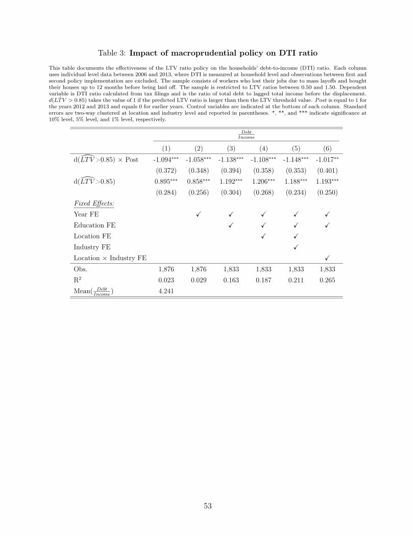
Table 3: Impact of macroprudential policy on DTI ratio

This table documents the effectiveness of the LTV ratio policy on the households’ debt-to-income (DTI) ratio. Each columnuses individual level data between 2006 and 2013, where DTI is measured at household level and observations between first andsecond policy implementation are excluded. The sample consists of workers who lost their jobs due to mass layoffs and boughttheir houses up to 12 months before being laid off. The sample is restricted to LTV ratios between 0.50 and 1.50. Dependentvariable is DTI ratio calculated from tax filings and is the ratio of total debt to lagged total income before the displacement.d( ˆLTV > 0.85) takes the value of 1 if the predicted LTV ratio is larger than then the LTV threshold value. Post is equal to 1 forthe years 2012 and 2013 and equals 0 for earlier years. Control variables are indicated at the bottom of each column. Standarderrors are two-way clustered at location and industry level and reported in parentheses. *, **, and *** indicate significance at10% level, 5% level, and 1% level, respectively.

DebtIncome

(1) (2) (3) (4) (5) (6)

d(LTV>0.85) × Post -1.094∗∗∗ -1.058∗∗∗ -1.138∗∗∗ -1.108∗∗∗ -1.148∗∗∗ -1.017∗∗

(0.372) (0.348) (0.394) (0.358) (0.353) (0.401)d(LTV>0.85) 0.895∗∗∗ 0.858∗∗∗ 1.192∗∗∗ 1.206∗∗∗ 1.188∗∗∗ 1.193∗∗∗

(0.284) (0.256) (0.304) (0.268) (0.234) (0.250)Fixed Effects:Year FE X X X X X

Education FE X X X X

Location FE X X

Industry FE X

Location × Industry FE X

Obs. 1,876 1,876 1,833 1,833 1,833 1,833R2 0.023 0.029 0.163 0.187 0.211 0.265Mean( Debt

Income) 4.241

53

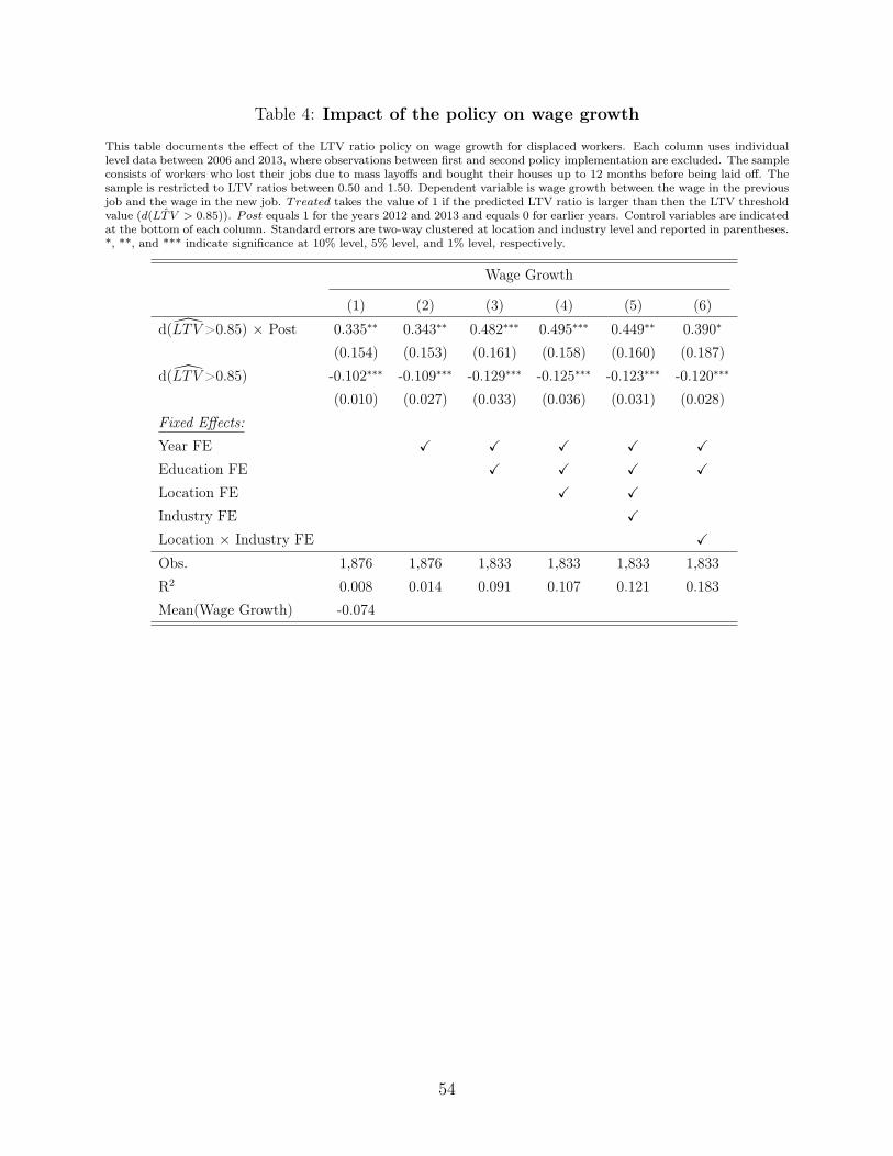
Table 4: Impact of the policy on wage growth

This table documents the effect of the LTV ratio policy on wage growth for displaced workers. Each column uses individuallevel data between 2006 and 2013, where observations between first and second policy implementation are excluded. The sampleconsists of workers who lost their jobs due to mass layoffs and bought their houses up to 12 months before being laid off. Thesample is restricted to LTV ratios between 0.50 and 1.50. Dependent variable is wage growth between the wage in the previousjob and the wage in the new job. Treated takes the value of 1 if the predicted LTV ratio is larger than then the LTV thresholdvalue (d( ˆLTV > 0.85)). Post equals 1 for the years 2012 and 2013 and equals 0 for earlier years. Control variables are indicatedat the bottom of each column. Standard errors are two-way clustered at location and industry level and reported in parentheses.*, **, and *** indicate significance at 10% level, 5% level, and 1% level, respectively.

Wage Growth

(1) (2) (3) (4) (5) (6)

d(LTV>0.85) × Post 0.335∗∗ 0.343∗∗ 0.482∗∗∗ 0.495∗∗∗ 0.449∗∗ 0.390∗

(0.154) (0.153) (0.161) (0.158) (0.160) (0.187)d(LTV>0.85) -0.102∗∗∗ -0.109∗∗∗ -0.129∗∗∗ -0.125∗∗∗ -0.123∗∗∗ -0.120∗∗∗

(0.010) (0.027) (0.033) (0.036) (0.031) (0.028)Fixed Effects:Year FE X X X X X

Education FE X X X X

Location FE X X

Industry FE X

Location × Industry FE X

Obs. 1,876 1,876 1,833 1,833 1,833 1,833R2 0.008 0.014 0.091 0.107 0.121 0.183Mean(Wage Growth) -0.074

54

Table 5: Impact of the policy on characteristics of the treated group

This table documents that the LTV ratio policy does not change the characteristics of the treated group. Each column usesindividual level data between 2006 and 2013, where observations between first and second policy implementation are excluded.The sample consists of workers who lost their jobs due to mass layoffs and bought their houses up to 12 months before being laidoff. The sample is restricted to LTV ratios between 0.50 and 1.50. Dependent variables are indicated at the column headings.All dependent variables are lagged by one period (i.e. one period before the layoff). d( ˆLTV > 0.85) takes the value of 1 ifthe predicted LTV ratio is larger than then the LTV threshold value. Post equals 1 for the years 2012 and 2013 and equals0 for earlier years. Control variables are indicated at the bottom of each column. Standard errors are two-way clustered atlocation and industry level and reported in parentheses. *, **, and *** indicate significance at 10% level, 5% level, and 1%level, respectively.

Previous Inc. Wage Buss. Inc. Trans. Unemp. Ben. Educ.

(1) (2) (3) (4) (5) (6)

d(LTV>0.85) × Post 0.042 0.061 0.183 -0.311 -0.043 0.031(0.191) (0.195) (0.141) (0.426) (0.243) (0.071)

d(LTV>0.85) 0.064 0.060 -0.050 0.022 0.105∗∗ 0.004(0.055) (0.055) (0.055) (0.085) (0.047) (0.019)

Fixed Effects:Year FE X X X X X X

Education FE X X X X X

Location FE X X X X X X

Industry FE X X X X X X

Obs. 1,833 1,833 1,833 1,833 1,833 1,876R2 0.110 0.109 0.080 0.120 0.093 0.083Mean(Dependent Var.) 0.361 0.369 0.092 0.333 0.050 0.777

55

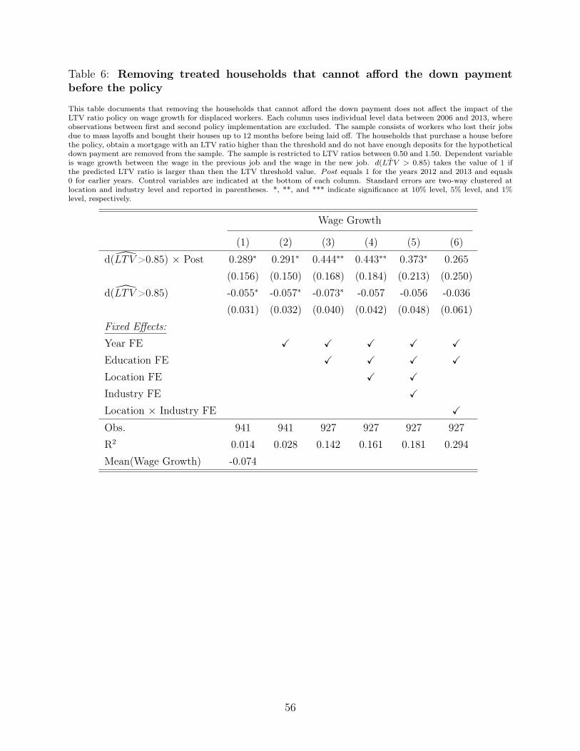
Table 6: Removing treated households that cannot afford the down paymentbefore the policy

This table documents that removing the households that cannot afford the down payment does not affect the impact of theLTV ratio policy on wage growth for displaced workers. Each column uses individual level data between 2006 and 2013, whereobservations between first and second policy implementation are excluded. The sample consists of workers who lost their jobsdue to mass layoffs and bought their houses up to 12 months before being laid off. The households that purchase a house beforethe policy, obtain a mortgage with an LTV ratio higher than the threshold and do not have enough deposits for the hypotheticaldown payment are removed from the sample. The sample is restricted to LTV ratios between 0.50 and 1.50. Dependent variableis wage growth between the wage in the previous job and the wage in the new job. d( ˆLTV > 0.85) takes the value of 1 ifthe predicted LTV ratio is larger than then the LTV threshold value. Post equals 1 for the years 2012 and 2013 and equals0 for earlier years. Control variables are indicated at the bottom of each column. Standard errors are two-way clustered atlocation and industry level and reported in parentheses. *, **, and *** indicate significance at 10% level, 5% level, and 1%level, respectively.

Wage Growth

(1) (2) (3) (4) (5) (6)

d(LTV>0.85) × Post 0.289∗ 0.291∗ 0.444∗∗ 0.443∗∗ 0.373∗ 0.265(0.156) (0.150) (0.168) (0.184) (0.213) (0.250)

d(LTV>0.85) -0.055∗ -0.057∗ -0.073∗ -0.057 -0.056 -0.036(0.031) (0.032) (0.040) (0.042) (0.048) (0.061)

Fixed Effects:Year FE X X X X X

Education FE X X X X

Location FE X X

Industry FE X

Location × Industry FE X

Obs. 941 941 927 927 927 927R2 0.014 0.028 0.142 0.161 0.181 0.294Mean(Wage Growth) -0.074

56

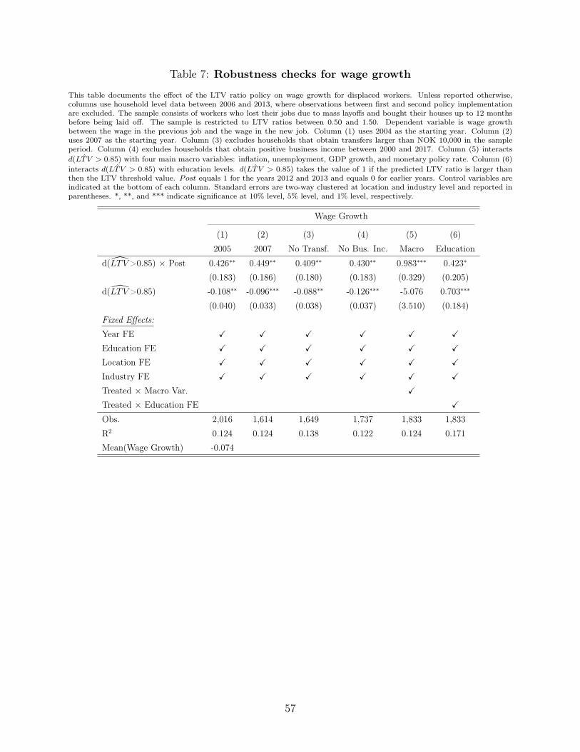
Table 7: Robustness checks for wage growth

This table documents the effect of the LTV ratio policy on wage growth for displaced workers. Unless reported otherwise,columns use household level data between 2006 and 2013, where observations between first and second policy implementationare excluded. The sample consists of workers who lost their jobs due to mass layoffs and bought their houses up to 12 monthsbefore being laid off. The sample is restricted to LTV ratios between 0.50 and 1.50. Dependent variable is wage growthbetween the wage in the previous job and the wage in the new job. Column (1) uses 2004 as the starting year. Column (2)uses 2007 as the starting year. Column (3) excludes households that obtain transfers larger than NOK 10,000 in the sampleperiod. Column (4) excludes households that obtain positive business income between 2000 and 2017. Column (5) interactsd( ˆLTV > 0.85) with four main macro variables: inflation, unemployment, GDP growth, and monetary policy rate. Column (6)interacts d( ˆLTV > 0.85) with education levels. d( ˆLTV > 0.85) takes the value of 1 if the predicted LTV ratio is larger thanthen the LTV threshold value. Post equals 1 for the years 2012 and 2013 and equals 0 for earlier years. Control variables areindicated at the bottom of each column. Standard errors are two-way clustered at location and industry level and reported inparentheses. *, **, and *** indicate significance at 10% level, 5% level, and 1% level, respectively.

Wage Growth

(1) (2) (3) (4) (5) (6)2005 2007 No Transf. No Bus. Inc. Macro Education

d(LTV>0.85) × Post 0.426∗∗ 0.449∗∗ 0.409∗∗ 0.430∗∗ 0.983∗∗∗ 0.423∗

(0.183) (0.186) (0.180) (0.183) (0.329) (0.205)d(LTV>0.85) -0.108∗∗ -0.096∗∗∗ -0.088∗∗ -0.126∗∗∗ -5.076 0.703∗∗∗

(0.040) (0.033) (0.038) (0.037) (3.510) (0.184)Fixed Effects:Year FE X X X X X X

Education FE X X X X X X

Location FE X X X X X X

Industry FE X X X X X X

Treated × Macro Var. X

Treated × Education FE X

Obs. 2,016 1,614 1,649 1,737 1,833 1,833R2 0.124 0.124 0.138 0.122 0.124 0.171Mean(Wage Growth) -0.074

57

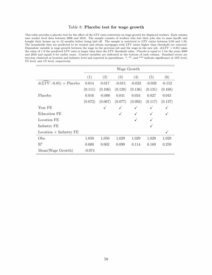
Table 8: Placebo test for wage growth

This table provides a placebo test for the effect of the LTV ratio restriction on wage growth for displaced workers. Each columnuses worker level data between 2006 and 2010. The sample consists of workers who lost their jobs due to mass layoffs andbought their houses up to 12 months before being laid off. The sample is restricted to LTV ratios between 0.50 and 1.50.The households that are predicted to be treated and obtain mortgages with LTV ratios higher than threshold are removed.Dependent variable is wage growth between the wage in the previous job and the wage in the new job. d( ˆLTV > 0.85) takesthe value of 1 if the predicted LTV ratio is larger than then the LTV threshold value. Placebo is equal to 1 for the years 2009and 2010 and equals 0 for earlier years. Control variables are indicated at the bottom of each column. Standard errors aretwo-way clustered at location and industry level and reported in parentheses. *, **, and *** indicate significance at 10% level,5% level, and 1% level, respectively.

Wage Growth

(1) (2) (3) (4) (5) (6)

d(LTV>0.85) × Placebo 0.014 0.017 -0.015 -0.033 -0.039 -0.152(0.111) (0.106) (0.128) (0.136) (0.131) (0.168)

Placebo 0.016 -0.000 0.041 0.034 0.027 0.045(0.072) (0.067) (0.077) (0.092) (0.117) (0.137)

Year FE X X X X X

Education FE X X X X

Location FE X X

Industry FE X

Location × Industry FE X

Obs. 1,050 1,050 1,029 1,029 1,029 1,029R2 0.000 0.002 0.099 0.114 0.169 0.259Mean(Wage Growth) -0.074

58

Table 9: Through what mechanism does leverage affect starting wages?

This table documents that LTV ratio restriction increases the displaced workers’ unemployment spells and firm wage premiumsof their new employers, but does not affect debt utilization during the unemployment spell. Columns (1)-(2) and (5)-(6) useindividual level and Columns (3) and (4) use household level data between 2006 and 2013, where observations between firstand second policy implementation are excluded. The sample consists of workers who lost their jobs due to mass layoffs andbought their houses up to 12 months before being laid off. The sample is restricted to LTV ratios between 0.50 and 1.50.Columns (1) and (2) use ln(Unemployment Spell) as the dependent variable. Columns (3) and (4) use ∆ln(Ex− Post Debt)(i.e. log change in household level debt after the year of displacement) as the dependent variable. Columns (5) and (6) use∆Firm Wage Premium (i.e. the difference of firm wage premiums between the old and new employer) as the dependentvariable. Firm wage premium is estimated using the AKM method (Abowd et al., 1999). d( ˆLTV > 0.85) takes the value of 1if the predicted LTV ratio is larger than then the LTV threshold value. Post equals 1 for the years 2012 and 2013 and equals0 for earlier years. Control variables are indicated at the bottom of each column. Standard errors are two-way clustered atlocation and industry level and reported in parentheses. *, **, and *** indicate significance at 10% level, 5% level, and 1%level, respectively.

ln(Unemp. Spell) ∆ ln(Ex-Post Debt) ∆ ln(Firm Wage Pre.)

(1) (2) (3) (4) (5) (6)

d(LTV>0.85) × Post 0.608∗∗∗ 0.567∗ -0.067 -0.114 0.004 0.058∗∗

(0.205) (0.281) (0.244) (0.313) (0.023) (0.027)d(LTV>0.85) 0.019 0.017 -0.023 -0.063 0.029∗∗∗ 0.009

(0.091) (0.110) (0.024) (0.057) (0.007) (0.008)Fixed Effects:Year FE X X X

Education FE X X X

Location FE X X X

Industry FE X X X

Obs. 1,876 1,833 1,876 1,833 1,672 1,637R2 0.006 0.160 0.000 0.096 0.002 0.386Mean(Dependent Var.) 2.270 0.085 -0.286

59

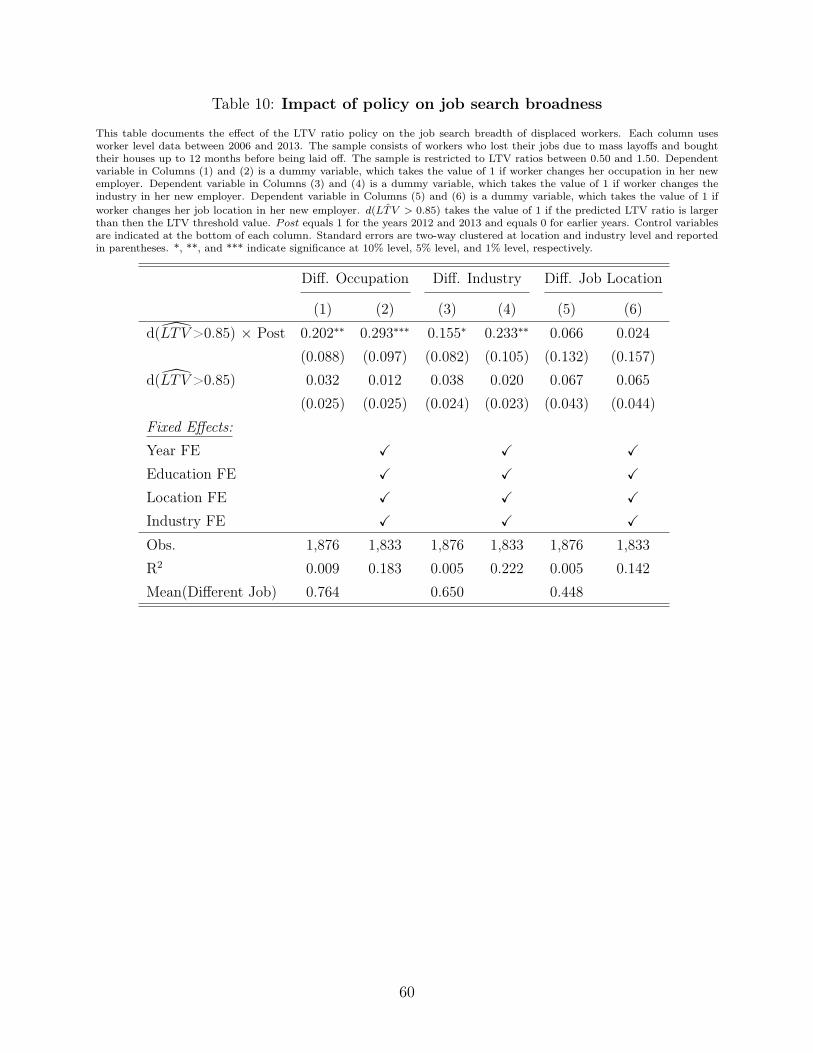
Table 10: Impact of policy on job search broadness

This table documents the effect of the LTV ratio policy on the job search breadth of displaced workers. Each column usesworker level data between 2006 and 2013. The sample consists of workers who lost their jobs due to mass layoffs and boughttheir houses up to 12 months before being laid off. The sample is restricted to LTV ratios between 0.50 and 1.50. Dependentvariable in Columns (1) and (2) is a dummy variable, which takes the value of 1 if worker changes her occupation in her newemployer. Dependent variable in Columns (3) and (4) is a dummy variable, which takes the value of 1 if worker changes theindustry in her new employer. Dependent variable in Columns (5) and (6) is a dummy variable, which takes the value of 1 ifworker changes her job location in her new employer. d( ˆLTV > 0.85) takes the value of 1 if the predicted LTV ratio is largerthan then the LTV threshold value. Post equals 1 for the years 2012 and 2013 and equals 0 for earlier years. Control variablesare indicated at the bottom of each column. Standard errors are two-way clustered at location and industry level and reportedin parentheses. *, **, and *** indicate significance at 10% level, 5% level, and 1% level, respectively.

Diff. Occupation Diff. Industry Diff. Job Location

(1) (2) (3) (4) (5) (6)

d(LTV>0.85) × Post 0.202∗∗ 0.293∗∗∗ 0.155∗ 0.233∗∗ 0.066 0.024(0.088) (0.097) (0.082) (0.105) (0.132) (0.157)

d(LTV>0.85) 0.032 0.012 0.038 0.020 0.067 0.065(0.025) (0.025) (0.024) (0.023) (0.043) (0.044)

Fixed Effects:Year FE X X X

Education FE X X X

Location FE X X X

Industry FE X X X

Obs. 1,876 1,833 1,876 1,833 1,876 1,833R2 0.009 0.183 0.005 0.222 0.005 0.142Mean(Different Job) 0.764 0.650 0.448

60

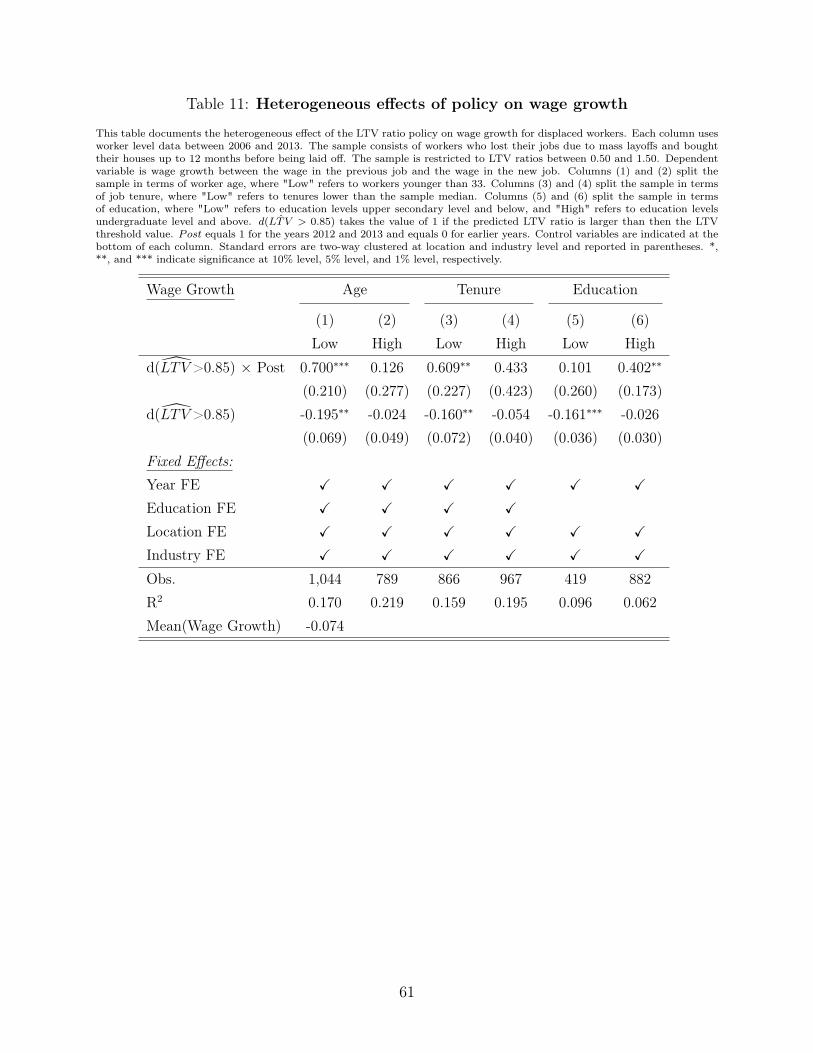
Table 11: Heterogeneous effects of policy on wage growth

This table documents the heterogeneous effect of the LTV ratio policy on wage growth for displaced workers. Each column usesworker level data between 2006 and 2013. The sample consists of workers who lost their jobs due to mass layoffs and boughttheir houses up to 12 months before being laid off. The sample is restricted to LTV ratios between 0.50 and 1.50. Dependentvariable is wage growth between the wage in the previous job and the wage in the new job. Columns (1) and (2) split thesample in terms of worker age, where "Low" refers to workers younger than 33. Columns (3) and (4) split the sample in termsof job tenure, where "Low" refers to tenures lower than the sample median. Columns (5) and (6) split the sample in termsof education, where "Low" refers to education levels upper secondary level and below, and "High" refers to education levelsundergraduate level and above. d( ˆLTV > 0.85) takes the value of 1 if the predicted LTV ratio is larger than then the LTVthreshold value. Post equals 1 for the years 2012 and 2013 and equals 0 for earlier years. Control variables are indicated at thebottom of each column. Standard errors are two-way clustered at location and industry level and reported in parentheses. *,**, and *** indicate significance at 10% level, 5% level, and 1% level, respectively.

Wage Growth Age Tenure Education

(1) (2) (3) (4) (5) (6)Low High Low High Low High

d(LTV>0.85) × Post 0.700∗∗∗ 0.126 0.609∗∗ 0.433 0.101 0.402∗∗

(0.210) (0.277) (0.227) (0.423) (0.260) (0.173)d(LTV>0.85) -0.195∗∗ -0.024 -0.160∗∗ -0.054 -0.161∗∗∗ -0.026

(0.069) (0.049) (0.072) (0.040) (0.036) (0.030)Fixed Effects:Year FE X X X X X X

Education FE X X X X

Location FE X X X X X X

Industry FE X X X X X X

Obs. 1,044 789 866 967 419 882R2 0.170 0.219 0.159 0.195 0.096 0.062Mean(Wage Growth) -0.074

61

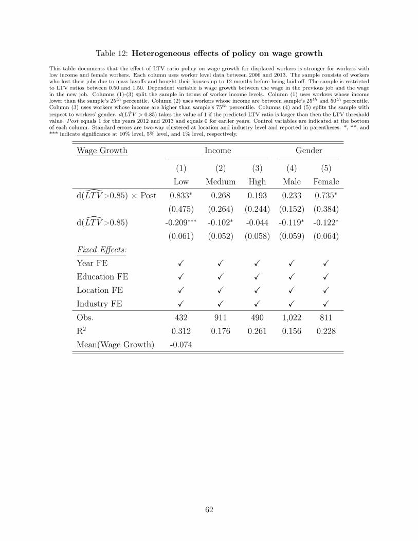
Table 12: Heterogeneous effects of policy on wage growth

This table documents that the effect of LTV ratio policy on wage growth for displaced workers is stronger for workers withlow income and female workers. Each column uses worker level data between 2006 and 2013. The sample consists of workerswho lost their jobs due to mass layoffs and bought their houses up to 12 months before being laid off. The sample is restrictedto LTV ratios between 0.50 and 1.50. Dependent variable is wage growth between the wage in the previous job and the wagein the new job. Columns (1)-(3) split the sample in terms of worker income levels. Column (1) uses workers whose incomelower than the sample’s 25th percentile. Column (2) uses workers whose income are between sample’s 25th and 50th percentile.Column (3) uses workers whose income are higher than sample’s 75th percentile. Columns (4) and (5) splits the sample withrespect to workers’ gender. d( ˆLTV > 0.85) takes the value of 1 if the predicted LTV ratio is larger than then the LTV thresholdvalue. Post equals 1 for the years 2012 and 2013 and equals 0 for earlier years. Control variables are indicated at the bottomof each column. Standard errors are two-way clustered at location and industry level and reported in parentheses. *, **, and*** indicate significance at 10% level, 5% level, and 1% level, respectively.

Wage Growth Income Gender

(1) (2) (3) (4) (5)Low Medium High Male Female

d(LTV>0.85) × Post 0.833∗ 0.268 0.193 0.233 0.735∗

(0.475) (0.264) (0.244) (0.152) (0.384)d(LTV>0.85) -0.209∗∗∗ -0.102∗ -0.044 -0.119∗ -0.122∗

(0.061) (0.052) (0.058) (0.059) (0.064)Fixed Effects:Year FE X X X X X

Education FE X X X X X

Location FE X X X X X

Industry FE X X X X X

Obs. 432 911 490 1,022 811R2 0.312 0.176 0.261 0.156 0.228Mean(Wage Growth) -0.074

62

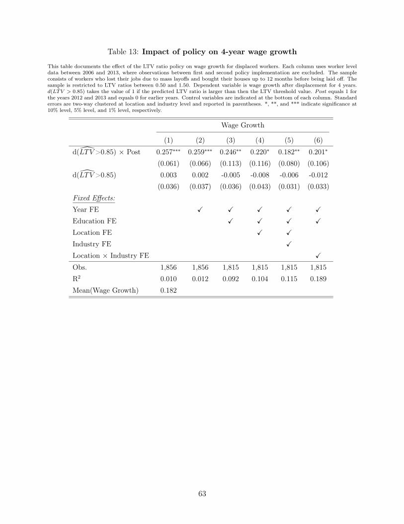
Table 13: Impact of policy on 4-year wage growth

This table documents the effect of the LTV ratio policy on wage growth for displaced workers. Each column uses worker leveldata between 2006 and 2013, where observations between first and second policy implementation are excluded. The sampleconsists of workers who lost their jobs due to mass layoffs and bought their houses up to 12 months before being laid off. Thesample is restricted to LTV ratios between 0.50 and 1.50. Dependent variable is wage growth after displacement for 4 years.d( ˆLTV > 0.85) takes the value of 1 if the predicted LTV ratio is larger than then the LTV threshold value. Post equals 1 forthe years 2012 and 2013 and equals 0 for earlier years. Control variables are indicated at the bottom of each column. Standarderrors are two-way clustered at location and industry level and reported in parentheses. *, **, and *** indicate significance at10% level, 5% level, and 1% level, respectively.

Wage Growth

(1) (2) (3) (4) (5) (6)

d(LTV>0.85) × Post 0.257∗∗∗ 0.259∗∗∗ 0.246∗∗ 0.220∗ 0.182∗∗ 0.201∗

(0.061) (0.066) (0.113) (0.116) (0.080) (0.106)d(LTV>0.85) 0.003 0.002 -0.005 -0.008 -0.006 -0.012

(0.036) (0.037) (0.036) (0.043) (0.031) (0.033)Fixed Effects:Year FE X X X X X

Education FE X X X X

Location FE X X

Industry FE X

Location × Industry FE X

Obs. 1,856 1,856 1,815 1,815 1,815 1,815R2 0.010 0.012 0.092 0.104 0.115 0.189Mean(Wage Growth) 0.182

63

Table 14: Impact of policy on households’ wage volatility

This table documents the effect of the LTV ratio policy on the displaced workers’ wage volatility. Each column uses worker leveldata between 2006 and 2013. The sample consists of workers who lost their jobs due to mass layoffs and bought their housesup to 12 months before being laid off. The sample is restricted to LTV ratios between 0.50 and 1.50. Dependent variable is thewage volatility of workers. Wage volatility is calculated by taking the standard deviation of annual wages for four years afterthe job displacement. d( ˆLTV > 0.85) takes the value of 1 if the predicted LTV ratio is larger than then the LTV thresholdvalue. Post equals 1 for the years 2012 and 2013 and equals 0 for earlier years. Control variables are indicated at the bottomof each column. Standard errors are two-way clustered at location and industry level and reported in parentheses. *, **, and*** indicate significance at 10% level, 5% level, and 1% level, respectively.

Wage Volatility

(1) (2) (3) (4) (5) (6)

d(LTV>0.85) × Post -26.274∗∗∗ -26.846∗∗∗ -32.215∗∗ -28.707∗ -24.719∗ -30.496∗∗

(5.917) (7.609) (15.242) (15.901) (12.988) (13.655)d(LTV>0.85) 1.033 1.294 4.282 5.332 5.183∗ 4.138

(3.270) (3.301) (3.211) (3.697) (2.635) (2.951)Fixed Effects:Year FE X X X X X

Education FE X X X X

Location FE X X

Industry FE X

Location × Industry FE X

Obs. 1,869 1,869 1,828 1,828 1,828 1,828R2 0.008 0.009 0.154 0.165 0.178 0.222Mean(Wage Volatility) 82.757

64

Appendix

A1 Impact of the LTV constraint on household leverage

In this section we detail the direct effect of the policy on households’ LTV, interest expenses,

and home purchases. Figure A5 shows γk from Equation 3 where we use the LTV ratio as the

dependent variable and provides visual evidence on the validity of the parallel trends assumptions

and the effectiveness of the policy. Relative to the pre-policy baseline year of 2009, the LTV

ratio of the treated and control groups evolves similarly in the pre-treatment period, supporting

the parallel trends assumption. After implementation of the macroprudential policy, the LTV

ratios of treated households’ fall significantly relative to the control group. Table A1, presents the

estimation results from the corresponding difference-in-differences model in Equation 2 and confirms

the visual intuition from Figure A5. Column (1) of Table A1 contains the parameter estimates

from a regression without any controls. The estimated treatment effect is highly significant and

negative treatment effect. The coefficient on the term d(LTV > 0.85)h×Postt implies that treated

households have a 23 percentage points lower LTV ratio after the policy. When we include, in

columns (2)-(6), year, education, location, industry, and location×industry fixed effects respectively

to control for unobservables, the estimated remains virtually unchanged. The d(LTV > 0.85)h

coefficient reflects that treated households had a 23 percentage points higher LTV ratios before the

introduction of the policy. Post treatment the treated and control groups have equal LTV ratios on

average.

The treatment effect we find is larger than what other studies, like Van Bekkum et al. (2019)

and Aastveit et al. (2020) find. Two circumstances account for this difference. First, we removed

households that obtain mortgages above the LTV threshold from the post-treatment period, because

they must be part of the exemption quota and therefore aren’t affected by the treatment. Second,

our baseline sample selection we allowed for a wider LTV ratio distribution. Both effects work in

the direction of increasing the relative decline in the LTV ratio of treated households.

Next we examine how the macroprudential policy achieves this debt-reducing effect. We there-

65

fore inspect how mortgage size, the price of purchased homes, and deposits change and again start

by considering the year-by-year effects in Figure A6. The visual evidence again supports the pres-

ence of parallel trends, for all three variables. We re-confirm the finding in the literature (Tzur-Ilan,

2020; Van Bekkum et al., 2019; Aastveit et al., 2020) that LTV constraints reduce mortgage size

(Figure A6a) and the cost of homes treated households buy (Figure A6b). A tighter borrowing

constraint does not reduce treated households’ liquidity by draining deposits Figure A6c. Table A2

indicates that treated household take on mortgages that are NOK 603,000 smaller mortgages to

pay for homes that are NOK 503,000 cheaper.41 In line with the lack of decline in deposits, we find

that the LTV restriction has a similar negative impact on household leverage when it is calculated

as (Total Debt - Deposits)/Income (Table A4).

Finally, we look into the policy’s influence on households’ cash flow. With smaller mortgages,

we expect interest payments to decrease mechanically. A reduction in risk may also induce banks

to charge a lower risk premium (Elul et al., 2010; Fuster and Willen, 2017; Ganong and Noel,

2020; Gupta and Hansman, 2020). Figure A7 confirms that treated and control groups behave

similarly before the treatment and that the treated group significantly reduces interest expenses

after the restriction. Table A3 indicates that interest payments fall by NOK 45,000 due to the policy.

Including principal repayments, we estimate that households’ annual cash outflow improves by NOK

65,000. This is economically sizable and equivalent to about 10 percent of treated households’ wages

before displacement and 65 percent of the median households’ deposits.

A2 Random Forest Algorithm

This section explains how we implement RF classification model. First, we describe data collecting

process. Then, we explain how we select the model parameters and hyperparameter tuning.

As explained in Section 3, we use several population registers. Merging these registers, we obtain

the following variables: income, wage, deposits, debt, unemployment benefits, business income,

age, education, location, and immigration status. Our data set allows us to observe the parents

41Households may be borrow less for the renovation of purchased homes, or reduce consumption to financehome related expenditures.

66

identifiers. Thus, we include parents’ income, wealth, deposits, debt, education, and immigration

status. Finally, to allow the model to consider macroeconomic conditions, we include GDP, inflation,

monetary policy rate, unemployment rate, and regional and national house prices. For balance

sheet variables (i.e. income, wage, deposits, unemployment benefits, business income, debt-to-

income ratio), we use household level information, which means that we use the total values of

these variables within the same household. For age, education, and immigration status, we use

information pertaining to the household’s main earner. Categorical variables (location, education,

and immigration status) are used as dummy variables for each category. Macro variables enter the

model both in levels and changes. We use national house price index to capture general housing

conditions. Moreover, using transactions data, we calculate the mean and median house prices for

each county and include both the levels and log changes of these values into the classification model.

The data period for the classification model is between 2002 and 2010. In this data period,

households can obtain mortgages without any restriction on LTV ratios. This allows us to label the

households as treated and control correctly (i.e. a household that obtains a mortgage with an LTV

ratio above 85 percent is classified as treated, vice versa). Moreover, we keep the first-time home

buyers whose LTV ratios are between 50 percent and 150 percent. Lastly, to reduce the overfitting

problem, we remove the regression sample from the classification sample. Overall, there are 261,151

observations used in the RF classification estimation.

The RF model is estimated by scikit − learn machine learning library for the Python pro-

gramming language. To select the model parameters, we use RandomizedSearchCV method for

hyperparameter tuning. In a nutshell, this method tries random values from a specified value set

and assigns score to these random values. Then, as a output, this method gives the parameters

that produce best out-of-sample results. In our case, the best parameters are n_estimators=200,

max_features=sqrt, min_samples_split=2, min_samples_leaf=8. After fitting the model,

the trained RF model is used to classify the regression sample.

ROC curve plot is a popular method to evaluate the performance of classification models for

binary labels. This plot has a true positive rate (proportion of treated units that are correctly

identified) on the y-axis, and a false positive rate (ratio of false treated to total control units). Each

67

dot represents the true and false positive rates for different probability threshold for treatment

assignment. For instance, if this threshold is set to 0, then every unit is classified as treated. This

means that the false positive rate is 1 since all negative events are classified as treated. Also, the

true positive rate is 1 since all true treated units are classified as treated. A successful classification

model has a lower decline in the true positive rate than the false positive rate as we lower the

probability threshold. In other words, closer a ROC curve is to the northwest of the plot, the more

successful it is. AUC is used to measure this success. Higher AUC values indicate that the model

is better in classifying the units, and a perfect model has AUC value of 1.

The scikit − learn library has a built in variable importance feature, which calculates the

importance by looking at the decrease in the mean impurity. However, this method can overstate

the importance of categorical variables with higher cardinality.42 Thus, we use permutation based

variable importance. The basic idea of this method is that a variable is more important if the

absence of this variable worsens the model’s performance more. First, we calculate the accuracy

of the classification model with all variables. Then, we remove each variable and calculate the

new accuracy. The reported scores are the percent decline in model’s accuracy when the variable is

removed (i. e. the model’s accuracy is 7 percent lower when household deposits variable is removed).

Macro variables enter to the model with levels and changes. House price variable includes national

house price index, mean and median of the regional house prices and their log changes of these

variables. The scores of the categorical variables are calculated by removing all the dummy variables

for that categorical variable.

A3 Placebo test

As explained in Section 4, we remove the households that are able to obtain mortgages with LTV

ratios above the threshold after the LTV restriction. The reason is that these households do not ex-

perience a reduction in their leverage, and they should thus not experience a change in their starting

wages. Even though this argument is reasonable, it might introduce bias into our estimations. We

42We plot the variable importance that uses built in function in Figure A8.

68

are able to observe and remove these households that are not affected by the restriction. However,

we cannot observe such households before the LTV restriction. Therefore, this removal can change

the composition of the treated group before and after the restriction. In Table 5, we show that the

characteristics of the treated group is not affected by the LTV restriction. However, there can still

be concerns about how this removal affects our estimations for starting wages.

To mitigate these concerns, we adopt a conservative strategy in our placebo test reported in

Table 8. That is, we remove the households that obtain mortgages with LTV ratio above the

threshold from the placebo post period. Doing this effectively removes the households that would not

be affected by the policy and obtain a mortgage with an LTV ratio above the threshold. However, the

removed part also includes the households whose LTV ratio would be lowered below the threshold.

Thus, there can be still concerns about how this removal affects the estimated coefficients.

We further mitigate the remaining concerns with a simulation-alike exercise. The ratio of house-

holds whose LTV ratios above the threshold after the policy is 20%. It is reasonable to assume that

the such households occur in the pre-treatment period with a similar ratio. To mimic the actual

sample in a more refined way, we randomly drop 20% of households whose LTV ratio above the

threshold from the placebo post period and repeat this for 10,000 times. If this removal creates a

bias in the starting wages regressions, then we should observe that a fraction of the estimations in

the simulation exercise has positive and significant. On the other hand, finding small and insignifi-

cant coefficients in this simulation exercise strongly support that this removal does not create a bias

in our results.

Figure A9 plots the distribution of the coefficients of d( ˆLTV > 0.85) × Placebo from this

simulation exercise. First observation is that the coefficients are centered around -0.03, which clearly

indicates that this removal does not create a bias. If anything, this exercise suggests a small and

negative bias that can attenuate our results. This finding holds for both a difference-in-differences

model without any controls (plain model) and a model with year, education, location, and industry

fixed effects (saturated model). Second, out of 10,000 estimations, none of them are significant at

10 percent for the plain model and only 4 of them are significant for the saturated model. Thus,

we conclude that this removal does not pose a threat for our estimations.

69

Figure A1: Macroeconomic conditions

This figure shows the macroeconomic conditions in Norway between 2000 and 2020. Figure A1a plots GDP growth, Figure A1bplots unemployment rate, Figure A1c plots inflation, and Figure A1d plots monetary policy rate. The orange line indicates thedate of the LTV ratio restriction.

-20

24

%

2000 2002 2004 2006 2008 2010 2012 2014 2016 2018 2020Year

GDP Growth

(a)

2.5

33.

54

4.5

%

2000 2002 2004 2006 2008 2010 2012 2014 2016 2018 2020Year

Unemployment Rate

(b)

01

23

4%

2000 2002 2004 2006 2008 2010 2012 2014 2016 2018 2020Year

Inflation

(c)

0.00

2.00

4.00

6.00

8.00

%

2000 2002 2004 2006 2008 2010 2012 2014 2016 2018 2020Year

Monetary Policy Rate

(d)

70

Figure A2: Regional house prices

This figure plots the regional house price growth rates for 9 largest counties. Blue dots show the house price growths ratesbefore the LTV restriction for 4 years. Orange dots show the house price growths rates after the LTV restriction for 2 years.

0.1

.20

.1.2

0.1

.2

Østfold Akershus Oslo

Buskerud Vestfold Rogaland

Hordaland Møre og Romsdal Trøndelag

Before LTV Restriction After LTV Restriction

Cha

nge

in H

ouse

Pric

es

71

Figure A3: Classification performance before the LTV ratio restriction

This figure plots the distribution of correctly and incorrectly classified households with respect to LTV ratios. Plot uses thesample before the LTV ratio restriction in which the correct treatment status is observed. Orange bars indicate the correctlyclassified households. Blue bars indicate the incorrectly classified households

Threshold

050

100

150

200

Freq

uenc

y

.5 1 1.5LTV

Correct Incorrect

72

Figure A4: Introduction of the macroprudential policy and house transactionvolume

This figure plots the house transaction volume over time. Vertical black dashed line indicates the announcement of the LTVrestriction. Vertical orange dashed line indicates the implementation of the LTV restriction.

Announcement Implementation

300

400

500

600

700

# of

Tra

nsac

tions

7/1/10 1/1/11 7/1/11 1/1/12 7/1/12 1/1/13Date

73

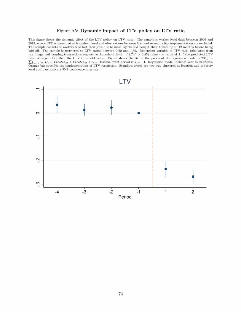
Figure A5: Dynamic impact of LTV policy on LTV ratio

This figure shows the dynamic effect of the LTV policy on LTV ratio. The sample is worker level data between 2006 and2013, where LTV is measured at household level and observations between first and second policy implementation are excluded.The sample consists of workers who lost their jobs due to mass layoffs and bought their houses up to 12 months before beinglaid off. The sample is restricted to LTV ratios between 0.50 and 1.50. Dependent variable is LTV ratio calculated fromtax filings and housing transactions register at household level. d( ˆLTV > 0.85) takes the value of 1 if the predicted LTVratio is larger than then the LTV threshold value. Figure shows the βs on the y-axis of the regression model, LTVht =∑2

k=−4 γk Dk × Treatedht + Treatedht + εht. Baseline event period is k = −1. Regression model includes year fixed effects.Orange bar specifies the implementation of LTV restriction. Standard errors are two-way clustered at location and industrylevel and bars indicate 95% confidence intervals.

-.3-.2

-.10

.1

-4 -3 -2 -1 1 2Period

LTV

74

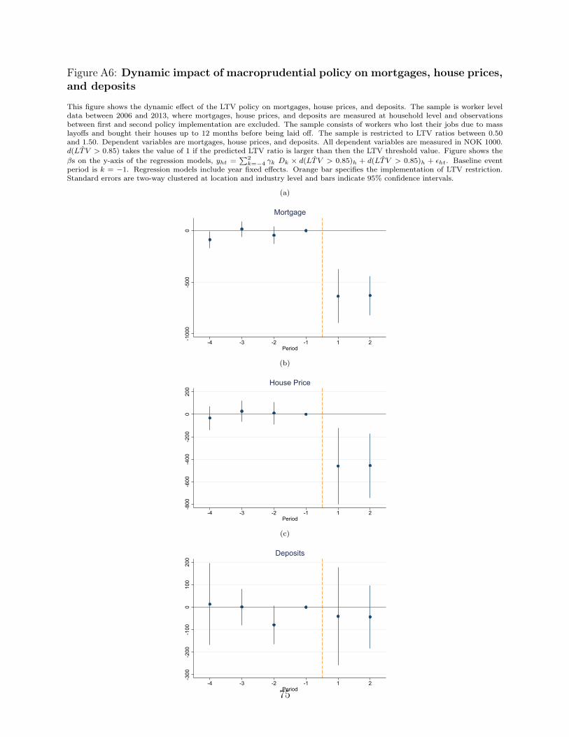
Figure A6: Dynamic impact of macroprudential policy on mortgages, house prices,and deposits

This figure shows the dynamic effect of the LTV policy on mortgages, house prices, and deposits. The sample is worker leveldata between 2006 and 2013, where mortgages, house prices, and deposits are measured at household level and observationsbetween first and second policy implementation are excluded. The sample consists of workers who lost their jobs due to masslayoffs and bought their houses up to 12 months before being laid off. The sample is restricted to LTV ratios between 0.50and 1.50. Dependent variables are mortgages, house prices, and deposits. All dependent variables are measured in NOK 1000.d( ˆLTV > 0.85) takes the value of 1 if the predicted LTV ratio is larger than then the LTV threshold value. Figure shows theβs on the y-axis of the regression models, yht =

∑2k=−4 γk Dk × d( ˆLTV > 0.85)h + d( ˆLTV > 0.85)h + εht. Baseline event

period is k = −1. Regression models include year fixed effects. Orange bar specifies the implementation of LTV restriction.Standard errors are two-way clustered at location and industry level and bars indicate 95% confidence intervals.

(a)-1

000

-500

0

-4 -3 -2 -1 1 2Period

Mortgage

(b)

-800

-600

-400

-200

020

0

-4 -3 -2 -1 1 2Period

House Price

(c)

-300

-200

-100

010

020

0

-4 -3 -2 -1 1 2Period

Deposits

75

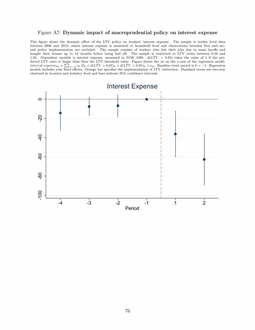
Figure A7: Dynamic impact of macroprudential policy on interest expense

This figure shows the dynamic effect of the LTV policy on workers’ interest expense. The sample is worker level databetween 2006 and 2013, where interest expense is measured at household level and observations between first and sec-ond policy implementation are excluded. The sample consists of workers who lost their jobs due to mass layoffs andbought their houses up to 12 months before being laid off. The sample is restricted to LTV ratios between 0.50 and1.50. Dependent variable is interest expense, measured in NOK 1000. d( ˆLTV > 0.85) takes the value of 1 if the pre-dicted LTV ratio is larger than then the LTV threshold value. Figure shows the βs on the y-axis of the regression model,interest expenseht =

∑2k=−4 γk Dk × d( ˆLTV > 0.85)h + d( ˆLTV > 0.85)h + εht. Baseline event period is k = −1. Regression

models includes year fixed effects. Orange bar specifies the implementation of LTV restriction. Standard errors are two-wayclustered at location and industry level and bars indicate 95% confidence intervals.

-100

-80

-60

-40

-20

0

-4 -3 -2 -1 1 2Period

Interest Expense

76

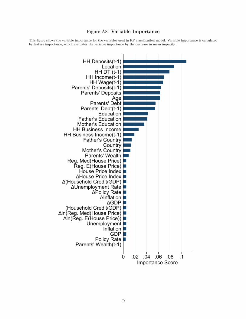
Figure A8: Variable Importance

This figure shows the variable importance for the variables used in RF classification model. Variable importance is calculatedby feature importance, which evaluates the variable importance by the decrease in mean impurity.

0 .02 .04 .06 .08 .1Importance Score

Parents' Wealth(t-1)Policy Rate

GDPInflation

Unemployment∆ln(Reg. E(House Price))

∆ln(Reg. Med(House Price)(Household Credit/GDP)

∆GDP∆Inflation

∆Policy Rate∆Unemployment Rate

∆(Household Credit/GDP)∆House Price Index

House Price IndexReg. E(House Price)

Reg. Med(House Price)Parents' Wealth

Mother's CountryCountry

Father's CountryHH Business Income(t-1)

HH Business IncomeMother's EducationFather's Education

EducationParents' Debt(t-1)

Parents' DebtAge

Parents' DepositsParents' Deposits(t-1)

HH Wage(t-1)HH Income(t-1)

HH DTI(t-1)Location

HH Deposits(t-1)

77

Figure A9: Simulation exercise for placebo test

This figure plots the coefficient distribution of d( ˆLTV > 0.85) × Placebo. In the placebo-post period, 20% of the householdsare removed randomly to mimic the design the main sample. Each histogram uses 10,000 draws. Orange bars use a plainmodel without any fixed effects. Blue bars use a model with year, education, location, and industry fixed effects. None of theestimated coefficients is significant in the plain model. Only four estimated coefficients are significant in the saturated model.

05

1015

Den

sity

-.15 -.1 -.05 0 .05

Plain Saturated

78

Table A1: Impact of macroprudential policy on LTV ratio

This table documents the effectiveness of the LTV ratio policy on the LTV ratios. Each column uses worker level data between2006 and 2013, where LTV is measured at household level and observations between first and second policy implementationare excluded. The sample consists of workers who lost their jobs due to mass layoffs and bought their houses up to 12 monthsbefore being laid off. The sample is restricted to LTV ratios between 0.50 and 1.50. Dependent variable is LTV ratio calculatedfrom tax filings and housing transactions register at household level.d( ˆLTV > 0.85) takes the value of 1 if the predicted LTVratio is larger than then the LTV threshold value. Post equals 1 for the years 2012 and 2013 and equals 0 for earlier years.Control variables are indicated at the bottom of each column. Standard errors are two-way clustered at location and industrylevel and reported in parentheses. *, **, and *** indicate significance at 10% level, 5% level, and 1% level, respectively.

LTV

(1) (2) (3) (4) (5) (6)

d(LTV>0.85) × Post -0.235∗∗∗ -0.234∗∗∗ -0.229∗∗∗ -0.225∗∗∗ -0.226∗∗∗ -0.218∗∗∗

(0.021) (0.021) (0.021) (0.017) (0.018) (0.030)d(LTV>0.85) 0.234∗∗∗ 0.233∗∗∗ 0.221∗∗∗ 0.216∗∗∗ 0.216∗∗∗ 0.212∗∗∗

(0.014) (0.014) (0.015) (0.015) (0.014) (0.019)Fixed Effects:Year FE X X X X X

Education FE X X X X

Location FE X X

Industry FE X

Location × Industry FE X

Obs. 1,876 1,876 1,833 1,833 1,833 1,833R2 0.211 0.213 0.278 0.290 0.291 0.343Mean(LTV) 0.924

79

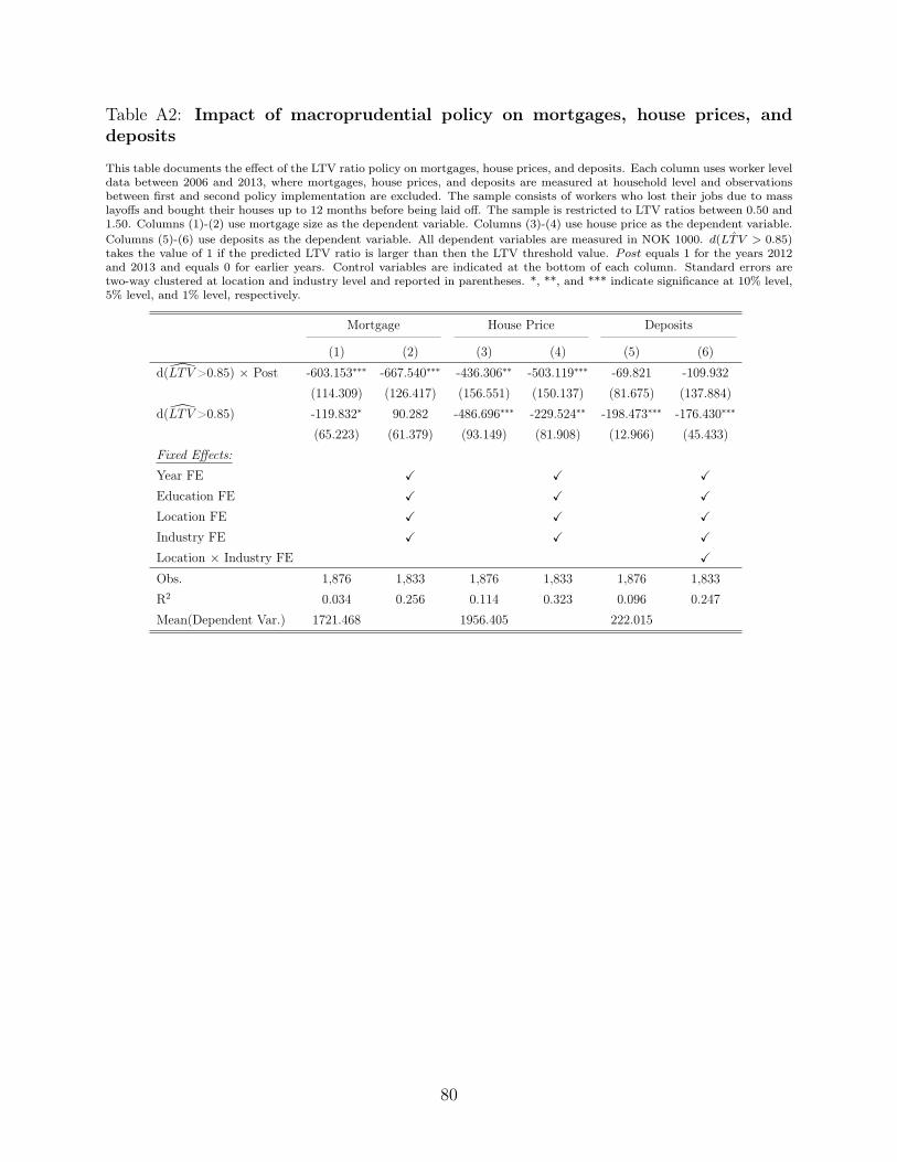
Table A2: Impact of macroprudential policy on mortgages, house prices, anddeposits

This table documents the effect of the LTV ratio policy on mortgages, house prices, and deposits. Each column uses worker leveldata between 2006 and 2013, where mortgages, house prices, and deposits are measured at household level and observationsbetween first and second policy implementation are excluded. The sample consists of workers who lost their jobs due to masslayoffs and bought their houses up to 12 months before being laid off. The sample is restricted to LTV ratios between 0.50 and1.50. Columns (1)-(2) use mortgage size as the dependent variable. Columns (3)-(4) use house price as the dependent variable.Columns (5)-(6) use deposits as the dependent variable. All dependent variables are measured in NOK 1000. d( ˆLTV > 0.85)takes the value of 1 if the predicted LTV ratio is larger than then the LTV threshold value. Post equals 1 for the years 2012and 2013 and equals 0 for earlier years. Control variables are indicated at the bottom of each column. Standard errors aretwo-way clustered at location and industry level and reported in parentheses. *, **, and *** indicate significance at 10% level,5% level, and 1% level, respectively.

Mortgage House Price Deposits

(1) (2) (3) (4) (5) (6)

d(LTV>0.85) × Post -603.153∗∗∗ -667.540∗∗∗ -436.306∗∗ -503.119∗∗∗ -69.821 -109.932(114.309) (126.417) (156.551) (150.137) (81.675) (137.884)

d(LTV>0.85) -119.832∗ 90.282 -486.696∗∗∗ -229.524∗∗ -198.473∗∗∗ -176.430∗∗∗

(65.223) (61.379) (93.149) (81.908) (12.966) (45.433)Fixed Effects:Year FE X X X

Education FE X X X

Location FE X X X

Industry FE X X X

Location × Industry FE X

Obs. 1,876 1,833 1,876 1,833 1,876 1,833R2 0.034 0.256 0.114 0.323 0.096 0.247Mean(Dependent Var.) 1721.468 1956.405 222.015

80

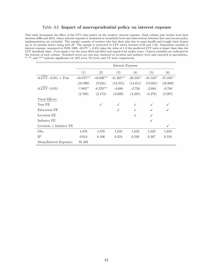
Table A3: Impact of macroprudential policy on interest expense

This table documents the effect of the LTV ratio policy on the workers’ interest expense. Each column uses worker level databetween 2006 and 2013, where interest expense is measured at household level and observations between first and second policyimplementation are excluded. The sample consists of workers who lost their jobs due to mass layoffs and bought their housesup to 12 months before being laid off. The sample is restricted to LTV ratios between 0.50 and 1.50. Dependent variable isinterest expense, measured in NOK 1000. d( ˆLTV > 0.85) takes the value of 1 if the predicted LTV ratio is larger than then theLTV threshold value. Post equals 1 for the years 2012 and 2013 and equals 0 for earlier years. Control variables are indicated atthe bottom of each column. Standard errors are two-way clustered at location and industry level and reported in parentheses.*, **, and *** indicate significance at 10% level, 5% level, and 1% level, respectively.

Interest Expense

(1) (2) (3) (4) (5) (6)

d(LTV>0.85) × Post -45.875∗∗∗ -44.626∗∗∗ -41.265∗∗∗ -36.504∗∗ -31.523∗∗ -37.456∗∗

(10.390) (9.821) (13.315) (14.011) (13.681) (16.988)d(LTV>0.85) -7.803∗∗ -8.570∗∗∗ -4.688 -2.726 -2.684 -0.780

(2.769) (2.173) (3.609) (4.285) (4.278) (5.007)Fixed Effects:Year FE X X X X X

Education FE X X X X

Location FE X X

Industry FE X

Location × Industry FE X

Obs. 1,876 1,876 1,833 1,833 1,833 1,833R2 0.014 0.106 0.224 0.249 0.267 0.316Mean(Interest Expense) 91.489

81

Table A4: Impact of policy on DTI ratio

This table documents the effectiveness of the LTV ratio policy on debt (net of deposits)-to-income (DTI) ratios. Each columnuses household level data between 2006 and 2013, where observations between first and second policy implementation areexcluded. The sample consists of workers who lost their jobs due to mass layoffs and bought their houses up to 12 monthsbefore being laid off. The sample is restricted to LTV ratios between 0.50 and 1.50. Dependent variable is DTI ratio calculatedfrom tax filings and is the ratio of total debt minus deposits to total income. d( ˆLTV > 0.85) takes the value of 1 if the predictedLTV ratio is larger than then the LTV threshold value. Post equals 1 for the years 2012 and 2013 and equals 0 for earlier years.Control variables are indicated at the bottom of each column. Standard errors are two-way clustered at location and industrylevel and reported in parentheses. *, **, and *** indicate significance at 10% level, 5% level, and 1% level, respectively.

Debt−Dep.Income

(1) (2) (3) (4) (5) (6)

d(LTV>0.85) × Post -1.035∗∗∗ -1.023∗∗∗ -0.986∗∗∗ -0.788∗∗ -0.934∗∗ -0.796(0.323) (0.339) (0.320) (0.337) (0.380) (0.480)

d(LTV>0.85) 0.793∗∗∗ 0.778∗∗∗ 0.866∗∗∗ 0.890∗∗∗ 0.884∗∗∗ 0.883∗∗∗

(0.119) (0.115) (0.127) (0.147) (0.143) (0.159)Fixed Effects:Year FE X X X X X

Education FE X X X X

Location FE X X

Industry FE X

Location × Industry FE X

Obs. 1,876 1,876 1,833 1,833 1,833 1,833R2 0.030 0.035 0.152 0.177 0.200 0.253Mean(Debt−Dep.

Income) 3.911

82

Table A5: Removing treated households that cannot afford the down paymentbefore the policy

This table documents that removing the households that cannot afford the down payment does not affect the impact of theLTV ratio policy on wage growth for displaced workers, after controlling for the available liquidity by including a cubic functionof the available liquidity. Each column uses individual level data between 2006 and 2013, where observations between first andsecond policy implementation are excluded. The sample consists of workers who lost their jobs due to mass layoffs and boughttheir houses up to 12 months before being laid off. The households that purchase a house before the policy, obtain a mortgagewith an LTV ratio higher than the threshold and do not have enough deposits for the hypothetical down payment are removedfrom the sample. The sample is restricted to LTV ratios between 0.50 and 1.50. Dependent variable is wage growth betweenthe wage in the previous job and the wage in the new job. d( ˆLTV > 0.85) takes the value of 1 if the predicted LTV ratio islarger than then the LTV threshold value. Post equals 1 for the years 2012 and 2013 and equals 0 for earlier years. Liquidity iscalculated as the deposits after taking out the down payment required by the LTV ratio restriction for pre- and post-treatmentperiods. Control variables are indicated at the bottom of each column. Standard errors are two-way clustered at location andindustry level and reported in parentheses. *, **, and *** indicate significance at 10% level, 5% level, and 1% level, respectively.

Wage Growth

(1) (2) (3) (4) (5) (6)

d(LTV>0.85) × Post 0.265∗ 0.274∗ 0.403∗∗ 0.397∗∗ 0.327∗ 0.193(0.142) (0.135) (0.160) (0.164) (0.183) (0.219)

d(LTV>0.85) -0.033 -0.041 -0.030 -0.013 -0.013 0.033(0.053) (0.052) (0.048) (0.050) (0.047) (0.062)

ln(liq.)t−1 0.248 0.204 0.287∗ 0.278∗ 0.345∗∗ 0.124(0.163) (0.161) (0.158) (0.151) (0.152) (0.144)

ln(liq.)t−1 × ln(liq.)t−1 -0.044 -0.037 -0.051∗ -0.049∗ -0.060∗∗ -0.025(0.026) (0.026) (0.026) (0.024) (0.025) (0.023)

ln(liq.)t−1 × ln(liq.)t−1 × ln(liq.)t−1 0.002∗ 0.002 0.002∗∗ 0.002∗∗ 0.003∗∗ 0.001(0.001) (0.001) (0.001) (0.001) (0.001) (0.001)

Fixed Effects:Year FE X X X X X

Education FE X X X X

Location FE X X

Industry FE X

Location × Industry FE X

Obs. 941 941 927 927 927 927R2 0.018 0.032 0.147 0.165 0.187 0.298Mean(Wage Growth) -0.074

83

Table A6: Impact of policy on wage growth

This table documents that wage growth of treated and control groups do not react to macroeconomic variables differently. Eachcolumn uses worker level data between 2006 and 2013, where observations between first and second policy implementation areexcluded. The sample consists of workers who lost their jobs due to mass layoffs and bought their houses up to 12 monthsbefore being laid off. The sample is restricted to LTV ratios between 0.50 and 1.50. Dependent variable is wage growth betweenthe wage in the previous job and the wage in the new job. d( ˆLTV > 0.85) takes the value of 1 if the predicted LTV ratio islarger than then the LTV threshold value. Post equals 1 for the years 2012 and 2013 and equals 0 for earlier years. Controlvariables are indicated at the bottom of each column. Standard errors are two-way clustered at location and industry level andreported in parentheses. *, **, and *** indicate significance at 10% level, 5% level, and 1% level, respectively.

Wage Growth

(1) (2) (3) (4) (5) (6)

d(LTV>0.85) × Post 0.744∗∗∗ 0.744∗∗∗ 1.030∗∗∗ 1.053∗∗∗ 0.983∗∗∗ 1.025∗

(0.154) (0.154) (0.325) (0.284) (0.329) (0.555)d(LTV>0.85) × Inflation -0.300∗∗ -0.300∗∗ -0.462 -0.476∗ -0.478∗ -0.589

(0.142) (0.142) (0.272) (0.249) (0.269) (0.522)d(LTV>0.85) × Unemployment 0.833 0.833 1.421 1.419 1.429 1.808

(0.541) (0.541) (1.032) (0.931) (1.018) (1.975)d(LTV>0.85) × GDP -0.185∗∗ -0.185∗∗ -0.278∗ -0.287∗ -0.280∗ -0.343

(0.081) (0.081) (0.159) (0.144) (0.160) (0.294)d(LTV>0.85) × Policy Rate 0.395∗ 0.395∗ 0.611 0.616∗ 0.610 0.754

(0.193) (0.193) (0.378) (0.335) (0.372) (0.692)d(LTV>0.85) -3.074 -3.074 -5.102 -5.073 -5.076 -6.370

(1.855) (1.855) (3.560) (3.182) (3.510) (6.698)Fixed Effects:Year FE X X X X X

Education FE X X X X

Location FE X X

Industry FE X

Location × Industry FE X

Obs. 1,876 1,876 1,833 1,833 1,833 1,833R2 0.017 0.017 0.095 0.111 0.124 0.186Mean(Wage Growth) -0.074

84

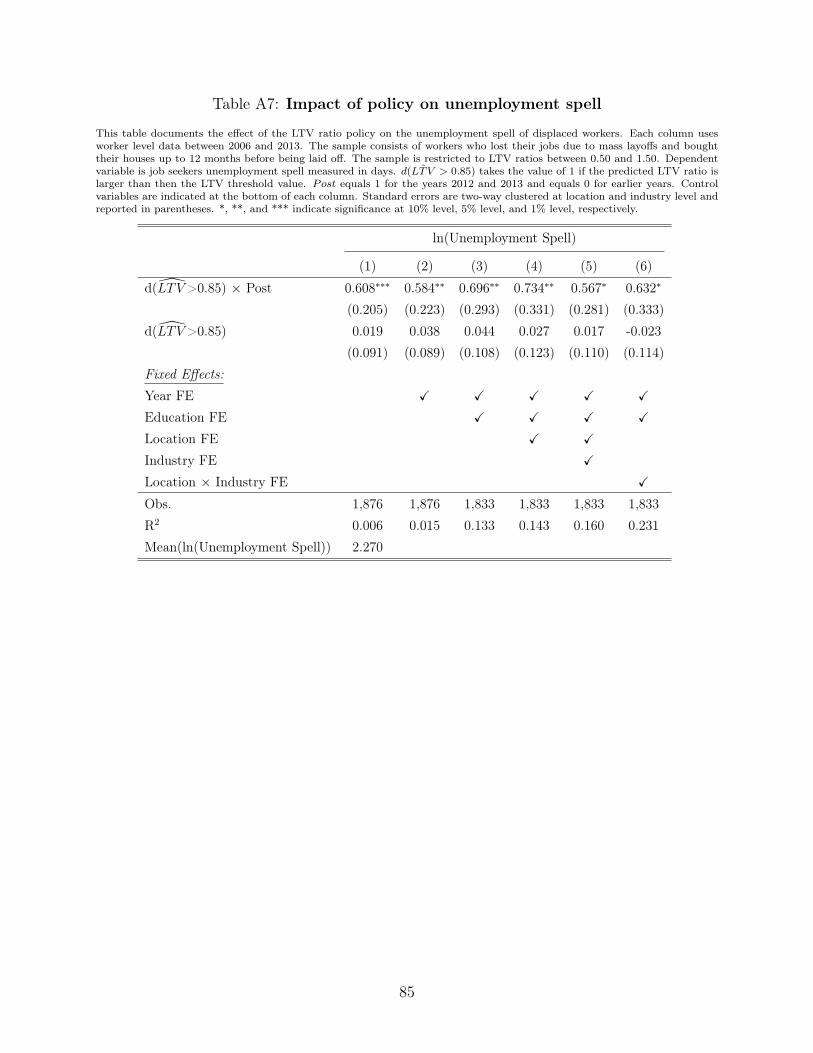
Table A7: Impact of policy on unemployment spell

This table documents the effect of the LTV ratio policy on the unemployment spell of displaced workers. Each column usesworker level data between 2006 and 2013. The sample consists of workers who lost their jobs due to mass layoffs and boughttheir houses up to 12 months before being laid off. The sample is restricted to LTV ratios between 0.50 and 1.50. Dependentvariable is job seekers unemployment spell measured in days. d( ˆLTV > 0.85) takes the value of 1 if the predicted LTV ratio islarger than then the LTV threshold value. Post equals 1 for the years 2012 and 2013 and equals 0 for earlier years. Controlvariables are indicated at the bottom of each column. Standard errors are two-way clustered at location and industry level andreported in parentheses. *, **, and *** indicate significance at 10% level, 5% level, and 1% level, respectively.

ln(Unemployment Spell)

(1) (2) (3) (4) (5) (6)

d(LTV>0.85) × Post 0.608∗∗∗ 0.584∗∗ 0.696∗∗ 0.734∗∗ 0.567∗ 0.632∗

(0.205) (0.223) (0.293) (0.331) (0.281) (0.333)d(LTV>0.85) 0.019 0.038 0.044 0.027 0.017 -0.023

(0.091) (0.089) (0.108) (0.123) (0.110) (0.114)Fixed Effects:Year FE X X X X X

Education FE X X X X

Location FE X X

Industry FE X

Location × Industry FE X

Obs. 1,876 1,876 1,833 1,833 1,833 1,833R2 0.006 0.015 0.133 0.143 0.160 0.231Mean(ln(Unemployment Spell)) 2.270

85

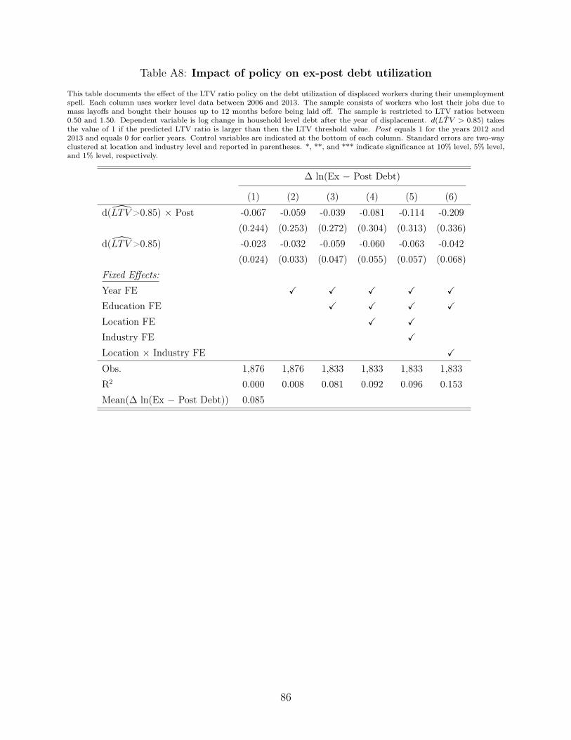
Table A8: Impact of policy on ex-post debt utilization

This table documents the effect of the LTV ratio policy on the debt utilization of displaced workers during their unemploymentspell. Each column uses worker level data between 2006 and 2013. The sample consists of workers who lost their jobs due tomass layoffs and bought their houses up to 12 months before being laid off. The sample is restricted to LTV ratios between0.50 and 1.50. Dependent variable is log change in household level debt after the year of displacement. d( ˆLTV > 0.85) takesthe value of 1 if the predicted LTV ratio is larger than then the LTV threshold value. Post equals 1 for the years 2012 and2013 and equals 0 for earlier years. Control variables are indicated at the bottom of each column. Standard errors are two-wayclustered at location and industry level and reported in parentheses. *, **, and *** indicate significance at 10% level, 5% level,and 1% level, respectively.

∆ ln(Ex − Post Debt)

(1) (2) (3) (4) (5) (6)

d(LTV>0.85) × Post -0.067 -0.059 -0.039 -0.081 -0.114 -0.209(0.244) (0.253) (0.272) (0.304) (0.313) (0.336)

d(LTV>0.85) -0.023 -0.032 -0.059 -0.060 -0.063 -0.042(0.024) (0.033) (0.047) (0.055) (0.057) (0.068)

Fixed Effects:Year FE X X X X X

Education FE X X X X

Location FE X X

Industry FE X

Location × Industry FE X

Obs. 1,876 1,876 1,833 1,833 1,833 1,833R2 0.000 0.008 0.081 0.092 0.096 0.153Mean(∆ ln(Ex − Post Debt)) 0.085

86

Table A9: Impact of policy on firm wage premium

This table documents the effect of the LTV ratio policy on the displaced workers’ employer’s firm wage premium. Each columnuses worker level data between 2006 and 2013. The sample consists of workers who lost their jobs due to mass layoffs and boughttheir houses up to 12 months before being laid off. The sample is restricted to LTV ratios between 0.50 and 1.50. Dependentvariable is the difference of firm wage premiums between the old and new employer. Firm wage premium is estimated usingAKM method (Abowd et al., 1999).d( ˆLTV > 0.85) takes the value of 1 if the predicted LTV ratio is larger than then the LTVthreshold value. Post equals 1 for the years 2012 and 2013 and equals 0 for earlier years. Control variables are indicated at thebottom of each column. Standard errors are two-way clustered at location and industry level and reported in parentheses. *,**, and *** indicate significance at 10% level, 5% level, and 1% level, respectively.

∆ ln(Firm Wage Premium)

(1) (2) (3) (4) (5) (6)

d(LTV>0.85) × Post 0.004 0.010 0.062 0.082∗∗∗ 0.058∗∗ 0.081∗∗

(0.023) (0.024) (0.000) (0.021) (0.027) (0.031)d(LTV>0.85) 0.029∗∗∗ 0.022∗∗ 0.012 0.008 0.009 0.010

(0.007) (0.009) (0.000) (0.009) (0.008) (0.009)Fixed Effects:Year FE X X X X X

Education FE X X X X

Location FE X X

Industry FE X

Location × Industry FE X

Obs. 1,672 1,672 1,637 1,637 1,637 1,637R2 0.002 0.042 0.193 0.228 0.386 0.472Mean(∆ ln(Firm Wage Premium)) -0.286

87

Table A10: Impact of policy on job types

This table documents that treated displaced workers switch to other occupations. Each column uses worker level data between2006 and 2013. The sample consists of workers who lost their jobs due to mass layoffs and bought their houses up to 12 monthsbefore being laid off. The sample is restricted to LTV ratios between 0.50 and 1.50. Dependent variable is a dummy variable,which takes the value of 1 if worker changes her occupation in her new employer. d( ˆLTV > 0.85) takes the value of 1 if thepredicted LTV ratio is larger than then the LTV threshold value. Post equals 1 for the years 2012 and 2013 and equals 0 forearlier years. Control variables are indicated at the bottom of each column. Standard errors are two-way clustered at locationand industry level and reported in parentheses. *, **, and *** indicate significance at 10% level, 5% level, and 1% level,respectively.

Different Occupation

(1) (2) (3) (4) (5) (6)

d(LTV>0.85) × Post 0.202∗∗ 0.206∗∗ 0.281∗∗∗ 0.316∗∗∗ 0.293∗∗∗ 0.253∗∗

(0.088) (0.093) (0.091) (0.094) (0.097) (0.118)d(LTV>0.85) 0.032 0.026 0.016 0.012 0.012 0.012

(0.025) (0.020) (0.018) (0.023) (0.025) (0.030)Fixed Effects:Year FE X X X X X

Education FE X X X X

Location FE X X

Industry FE X

Location × Industry FE X

Obs. 1,876 1,876 1,833 1,833 1,833 1,833R2 0.009 0.028 0.137 0.153 0.183 0.261Mean(Different Job) 0.764

88

Table A11: Impact of policy on industry switch

This table documents that treated displaced workers switch to other industries. Each column uses worker level data between2006 and 2013, where observations between first and second policy implementation are excluded. The sample consists of workerswho lost their jobs due to mass layoffs and bought their houses up to 12 months before being laid off. The sample is restrictedto LTV ratios between 0.50 and 1.50. Dependent variable is a dummy variable which takes the value of 1 if the household staysin the same industry. Industry is measured at 2-digit NAICS code level. d( ˆLTV > 0.85) takes the value of 1 if the predictedLTV ratio is larger than then the LTV threshold value. Post equals 1 for the years 2012 and 2013 and equals 0 for earlier years.Control variables are indicated at the bottom of each column. Standard errors are two-way clustered at location and industrylevel and reported in parentheses. *, **, and *** indicate significance at 10% level, 5% level, and 1% level, respectively.

Different Industry

(1) (2) (3) (4) (5) (6)

d(LTV>0.85) × Post 0.155∗ 0.166∗ 0.184∗ 0.211∗ 0.233∗∗ 0.178∗

(0.082) (0.082) (0.093) (0.103) (0.105) (0.103)d(LTV>0.85) 0.038 0.026 0.021 0.023 0.020 0.015

(0.024) (0.021) (0.020) (0.023) (0.023) (0.022)Fixed Effects:Year FE X X X X X

Education FE X X X X

Location FE X X

Industry FE X

Location × Industry FE X

Obs. 1,876 1,876 1,833 1,833 1,833 1,833R2 0.005 0.053 0.173 0.183 0.222 0.301Mean(Different Industry) 0.650

89

Table A12: Impact of policy on labor mobility

This table documents that treated displaced workers do not switch to other working places. Each column uses worker level databetween 2006 and 2013, where observations between first and second policy implementation are excluded. The sample consistsof workers who lost their jobs due to mass layoffs and bought their houses up to 12 months before being laid off. The sampleis restricted to LTV ratios between 0.50 and 1.50. Dependent variable is a dummy variable which takes the value of 1 if thehousehold stays in the same working place measured at municipality level. d( ˆLTV > 0.85) takes the value of 1 if the predictedLTV ratio is larger than then the LTV threshold value. Post equals 1 for the years 2012 and 2013 and equals 0 for earlier years.Control variables are indicated at the bottom of each column. Standard errors are two-way clustered at location and industrylevel and reported in parentheses. *, **, and *** indicate significance at 10% level, 5% level, and 1% level, respectively.

Different Job Location

(1) (2) (3) (4) (5) (6)

d(LTV>0.85) × Post 0.066 0.063 0.026 0.052 0.024 0.046(0.132) (0.133) (0.137) (0.151) (0.157) (0.170)

d(LTV>0.85) 0.067 0.066 0.064 0.065 0.065 0.062(0.043) (0.040) (0.051) (0.045) (0.044) (0.049)

Fixed Effects:Year FE X X X X X

Education FE X X X X

Location FE X X

Industry FE X

Location × Industry FE X

Obs. 1,876 1,876 1,833 1,833 1,833 1,833R2 0.005 0.016 0.097 0.136 0.142 0.214Mean(Labor Mobility) 0.448

90

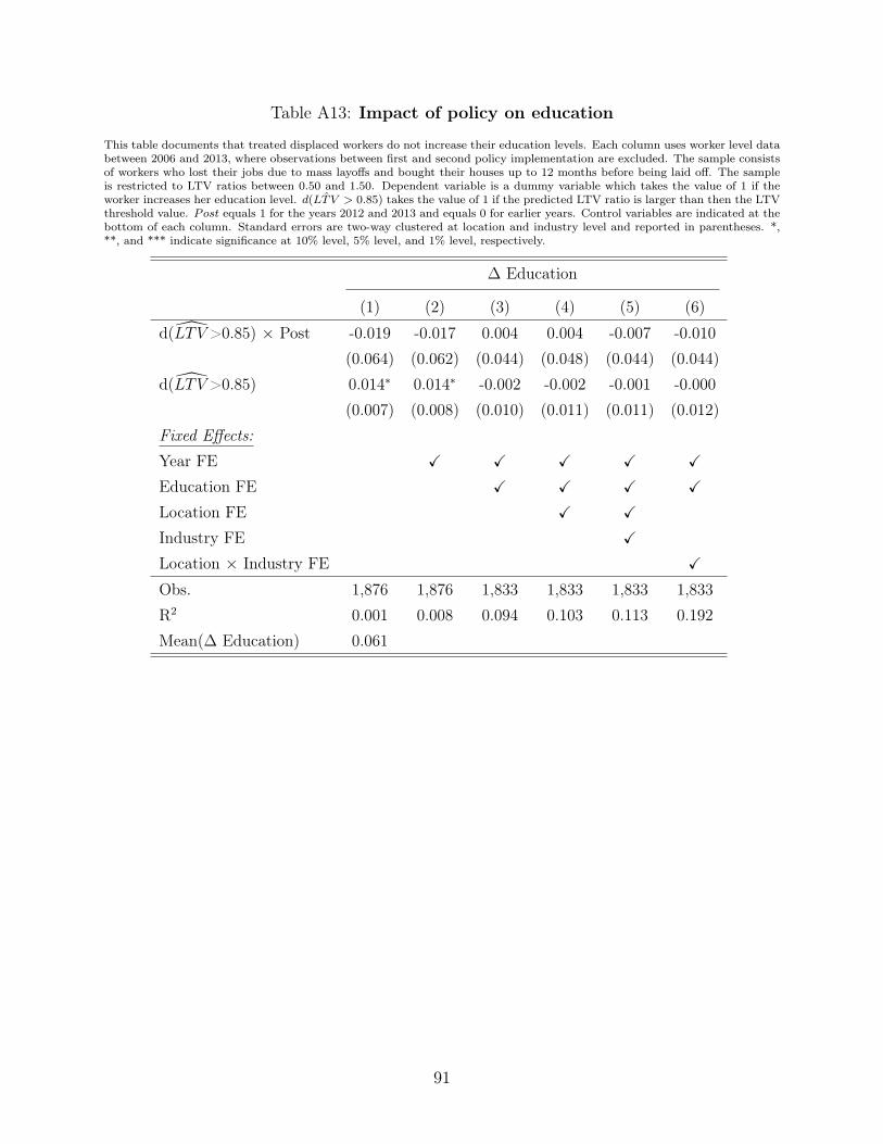
Table A13: Impact of policy on education

This table documents that treated displaced workers do not increase their education levels. Each column uses worker level databetween 2006 and 2013, where observations between first and second policy implementation are excluded. The sample consistsof workers who lost their jobs due to mass layoffs and bought their houses up to 12 months before being laid off. The sampleis restricted to LTV ratios between 0.50 and 1.50. Dependent variable is a dummy variable which takes the value of 1 if theworker increases her education level. d( ˆLTV > 0.85) takes the value of 1 if the predicted LTV ratio is larger than then the LTVthreshold value. Post equals 1 for the years 2012 and 2013 and equals 0 for earlier years. Control variables are indicated at thebottom of each column. Standard errors are two-way clustered at location and industry level and reported in parentheses. *,**, and *** indicate significance at 10% level, 5% level, and 1% level, respectively.

∆ Education

(1) (2) (3) (4) (5) (6)

d(LTV>0.85) × Post -0.019 -0.017 0.004 0.004 -0.007 -0.010(0.064) (0.062) (0.044) (0.048) (0.044) (0.044)

d(LTV>0.85) 0.014∗ 0.014∗ -0.002 -0.002 -0.001 -0.000(0.007) (0.008) (0.010) (0.011) (0.011) (0.012)

Fixed Effects:Year FE X X X X X

Education FE X X X X

Location FE X X

Industry FE X

Location × Industry FE X

Obs. 1,876 1,876 1,833 1,833 1,833 1,833R2 0.001 0.008 0.094 0.103 0.113 0.192Mean(∆ Education) 0.061

91