HOUSING INEQUALITY …davidalbouy.net/housinginequality.pdf · 1 Introduction In this paper, we examine a dimension of inequality that has received surprisingly scant attention {

NBER WORKING PAPER SERIES

HOUSING INEQUALITY

David AlbouyMike Zabek

Working Paper 21916http://www.nber.org/papers/w21916

NATIONAL BUREAU OF ECONOMIC RESEARCH1050 Massachusetts Avenue

Cambridge, MA 02138January 2016

We want to thank John Bound, Charles Brown, Gabriel Ehrlich, Enrico Moretti, Matthew Shapiro,Jeff Smith, and Bryan Stuart for valuable comments and suggestions. This research was supportedby a grant to Zabek via the Population Studies Center at the University of Michigan (R24 HD041028)and in part through computational resources and services provided by Advanced Research Computingat the University of Michigan, Ann Arbor. The views expressed herein are those of the authors anddo not necessarily reflect the views of the National Bureau of Economic Research.

NBER working papers are circulated for discussion and comment purposes. They have not been peer-reviewed or been subject to the review by the NBER Board of Directors that accompanies officialNBER publications.

© 2016 by David Albouy and Mike Zabek. All rights reserved. Short sections of text, not to exceedtwo paragraphs, may be quoted without explicit permission provided that full credit, including © notice,is given to the source.

Housing InequalityDavid Albouy and Mike ZabekNBER Working Paper No. 21916January 2016JEL No. D63

ABSTRACT

Inequality in U.S. housing prices and rents both declined in the mid-20th century, even as home-ownershiprates rose. Subsequently, housing-price inequality has risen to pre-War levels, while rent inequalityhas risen less. Combining both measures, we see inequality in housing consumption equivalents mirroringpatterns in income across both space and time, according to an income elasticity of housing demandjust below one. These patterns occur mainly within cities, and are not explained by observed changesin dwelling characteristics or locations. Instead, recent increases in housing inequality are driven mostby changes in the relative value of locations, seen especially through land.

David AlbouyDepartment of EconomicsUniversity of Illinois at Urbana-Champaign214 David Kinley HallUrbana, IL 61801-3606and [email protected]

Mike ZabekDepartment of EconomicsUniversity of Michigan611 Tappan St,Ann Arbor, MI [email protected]

1 Introduction

In this paper, we examine a dimension of inequality that has received surprisingly scant attention

– inequality in housing outcomes. We find that measures of inequality in housing prices and

rents in the United States exhibit a U-shaped pattern over the last 85 years, resembling patterns

of income and wealth inequality, often referred to as a “great compression” followed by a “great

divergence” (Piketty and Saez (2003), Saez and Zucman (2014)). Housing-value inequality fell

from 1930 to 1970 as home ownership expanded, but has subsequently risen. Rent inequality

also fell, but it has risen only slightly since. Combining both measures into a rental equivalent,

we again see a U-shape.

To understand the fall and subsequent rise of housing inequality, we use decomposition

techniques to quantify the impacts of key variables. Changes in housing inequality have occurred

primarily within cities and are not explained by observable changes in dwelling characteristics.

Thus, changes in the desirability of particular neighborhoods, reflected in land values, appear to

be the main contributor to changes in housing inequality, although we cannot rule out changes

in unobserved housing quality. Using a series of simple regressions, we also find that local

housing inequality is related with local income inequality at magnitudes implied by reasonable

values for the income elasticity of housing consumption.

Knowledge of housing inequality sheds light on larger issues concerning consumption and

wealth inequality. It informs debate over whether consumption inequality has grown as much as

income inequality over the last few decades.1 Housing accounts for a large share of consumption,

and has done so more stably than other items, such as food or health care.2 Housing may

represent permanent income particularly well as it is durable (Friedman (1957), p 208). The

great compression and great divergence in housing inequality are of roughly similar magnitude,

commensurate with income changes. However, housing inequality has less to do with tangible

dwelling characteristics — such as living space — and more to do with what people pay to live

1Krueger and Perri (2006) and Meyer and Sullivan (2010) argue that consumption inequality has increasedmuch less than income inequality using the Consumer Expenditure Survey. Aguiar and Bils (2011) propose acorrection for measurement error that results in a consumption inequality measure that mirrors income. Workusing PSID consumption measures by Attanasio and Pistaferri (2014) and earlier evidence by Cutler and Katz(1992) also suggest that consumption inequality has increased in line with income inequality.

2As a fraction of Personal Consumption Expenditures (PCE), “Housing and utilities” rose from 16.6 to18.1 percent between 1959 and 2014. Similar fractions for “Food and beverages purchases for off-premisesconsumption” are 19.4 to 7.5 percent; “Clothing and footwear,” 8.0 to 3.1 percent, ”Motor vehicles and parts,”5.9 to 3.7 percent; “Health care,” 4.7 to 16.5 percent. Depending on the survey, the budget share of housingroughly one-sixth, in the PCE, to one-third, in the Consumer Expenditure Survey (CEX), of average consumerexpenditures (Albouy and Lue (2015).)

1

in different locations. These locations offer different “intangibles” such as access to employment

and local amenities, such as schools, safety, and natural features.

There has also been recent debate over whether wealth inequality has increased as much as

income inequality.3 Housing informs this debate as it accounts for much of the overall capital

stock and is the principal asset for most Americans with savings.4 Our evidence that housing

values have diverged indirectly supports the view that wealth inequality has increased, albeit

to levels lower than before World War II, due to increases in home-ownership.5

To our knowledge, our paper is the first to document inequality in housing prices and rents

over such a long period and to relate them to measures of income inequality over space and time.

Our analysis of housing expenditures sheds light on consumption inequality prior to World War

II – before widely available household-level consumption data – providing direct evidence of a

great compression in consumption inequality contemporaneous with similar changes in income

and wealth.6 While several studies (e.g. Van Nieuwerburgh and Weill (2010), Moretti (2013),

and Gyourko, Mayer and Sinai (2013)) have examined recent changes in housing-price inequality

across cities, our analysis extends for longer, covers rents, and examines dwelling characteristics

and variation in prices within cities.

2 Data, Inequality Measures, and Empirical Techniques

2.1 Housing Data and Sample Selection

Our data are drawn from the full 1930 and 1940 Census, the long form of the 1960 through 2000

Censuses, and the American Community Survey (ACS) for 2009-12. These surveys ask owners

to report the current value of their home and renters to report their monthly rent. Renters from

1970 onward and home owners from 1980 onward also report their utility costs. Home values

3Kopczuk (2004) find a great compression of wealth inequality but little divergence afterwards. Using capi-talization methods, Saez and Zucman (2014) find greater divergence, although Kopczuk (2015) disputes this.

4Housing accounts for roughly one third of total household wealth and roughly 40 percent of the capital stock.Housing is almost two thirds of wealth for the middle three quintiles (Wolff, 2014). In 2004, 62 percent of housingwealth was held by the bottom 90 percent, and only 9.8 percent by the top 1 percent; for stocks and mutualfunds, the comparable numbers are 14.6 and 44.8 percent (Wolff 2009, p. 160).

5Differences in wealth due to inequality in housing values have more complex implications than differences dueto other types of capital. An appreciation in home prices will only increase a home-owner’s permanent wealth ifthey have a less expensive alternative to living in their now more expensive house. Rognlie (2014) and Bonnetet al. (2014) have emphasized this point in critiquing Piketty and Zucman (2014). One interesting feature of ourpaper is our finding that home owners have alternatives that are observably quite similar but much less expensive.This suggests that the distinction is less important.

6Goldin and Margo (1992) used methods similar to ours to highlight and examine the great compressionin incomes in the 1930’s and 1940’s. Piketty and Saez (2003) examine the great compression of top incomes,particularly from capital.

2

are recorded as intervals from 1960 through 2000 and monthly rents are reported as intervals

for 1960, 1980, and 1990. In all other years the questions record a continuous measure with

relatively little top coding.7

We restrict our sample to focus on residential homes and to maximize consistency across

years. This involves three restrictions. First, we restrict the sample to the continental United

States. Second, we eliminate all farms and homes used for commercial activities, such as

dental and medical offices. Fourth, we remove owner-occupied units in multi-family structures.

Appendix table A.1 lists the number of houses in each category. We remove farms in all years,

which is our most important sample restriction. The 1930 and 1940 data do not include dwelling

characteristics, nor do they indicate the presence of businesses, so we cannot remove businesses

and multi-family structures in these years. These two categories account for only 6 percent of

owner-occupied houses in 1960.8

2.2 Interpolation and Extrapolation Procedures

The Census often asks questions about home values and rents in terms of intervals. Even when

questions are asked in terms of continuous dollars, the data are top coded, and respondents

often round. To account for these issues, we use a Pareto interpolation procedure to allocate

responses within intervals. Where y are values distributed according to F (y), this procedure

fits ln[1− F (y)] = αj [ln(kj)− ln(y)], where αj > 1, kj > 0 are parameters for an interval j. In

other words, it fits a linear spline of the “tail” function ln[1−F (y)] to ln(y). For high values of

y, the αj parameters are fairly constant, implying that the Pareto distribution provides a good

fit. To improve comparability and handle rounding problems, we also interpolate in years with

continuous data, using 25 artificial intervals, with 4 percent of the data in each.9

At the top of the distribution, we use standard Pareto extrapolation procedures (e.g. Atkin-

son, Piketty and Saez (2011)). In years that we have information about the mean of top coded

values, we use the estimate of αJ = E[y|y > k]/(E[y|y > k]−k). In other years, we extrapolate

αJ for the top coded bin from the αj from intervals in the top 10 percent of the distribution.10

7The home value is the owner’s estimate. We discuss below how question changes impact our analysis. Wetake data from the ACS from 2009 (not 2008) through 2012 to reflect conditions after the latest housing boomand bust.

8Enumerator instructions for 1940 instruct respondents to exclude the value of units rented out and to alsoexclude the area of the house that is used for business purposes if this is a “considerable portion” of the house.These instructions are re-printed in the data appendix.

9Because of rounding, these intervals can sometimes contain only one value. In these cases, we decrease thenumber of groups until each interval has a top value at least 2.5 percent higher than its bottom value.

10The one exception to this are rent values in 1930 and 1940, where we hard code the top Pareto distribution

3

For the bottom interval we extrapolate values using a uniform distribution to deal with bottom

coding and problems associated with zero values. We set the minimum of this interval as a

proportion of average household income in that year. More details are in Appendix B.

2.3 House Values, Gross Rents, and Consumption Equivalents

We present all of our results separately for housing prices and rents. To integrate the two and

account for changes in home ownership (which mainly changed from 1940 to 1960), we impute

a rental equivalent measure for home owners, based on a constant user cost of 0.0785 times

the value of the house and plus utility payments.11 We then divide these rental measures by a

household equivalence scale to provide a per-person measure of housing consumption.12

2.4 Inequality Measures

To describe inequality in housing expenditures we use three scale and population invariant mea-

sures: the variance of logs, the Gini coefficient, and the Theil entropy index.13 We decompose

the variance of logs and the Theil index to show how much overall inequality is due to variation

across versus within areas. Note that the variance of logs is particularly sensitive to the bottom

of the distribution while the Gini coefficient and Theil mainly measure changes in the middle

of the distribution (Atkinson (1970)).

parameter to be 2.5. In these years we have a continuous distribution of rents (and home values) with very fewtop codes; parameters estimated from the mean procedure lead to suspiciously high inequality statistics.

11This commonly-used value is based on Peiser and Smith (1985). User costs of home ownership are foregoneinterest, depreciation, and property taxes, minus price appreciation. User costs vary over space, time, and possiblyoccupant, but there are various empirical and conceptual challenges in calculating year-by-city user costs (e.g.those examined in Verbrugge (2008) and Poterba and Sinai (2008)). We choose a constant number so as to avoidthe data being overly influenced by our choice of methodology, recognizing that scale invariance of the inequalitymeasures will help to undo differences among owners.

12Equivalence scales are designed to take into account economies of scale in consumption, such as from thesharing of common spaces, kitchens, etc. We use the OECD equivalence scale: 1 + 0.7(A− 1) + 0.5C where A isthe total number of adults in the household and C is the number of children (14 years old or below).

13The Theil index is computed by taking a weighted average of the log of the (normalized) expenditure onhousing by each household. Where y ≡ E[yi]:

T =1

N

N∑i=1

[yiy

ln

(yiy

)]The Gini coefficient and Theil index satisfy the principle of transfers, so a transfer from a rich to a poor personalways decreases inequality. We decompose Theil entropy indices and variances of logs by calling inequality inmean levels of housing expenditures across areas the between (areas) component, and inequality within areas thewithin component. As Cowell (2011) notes, the variance of logs is only decomposable with constant means oflogged values, not levels.

4

2.5 Dwelling Characteristics and Location Measures

Dwelling characteristics are provided only from 1960 onwards. They include the age of the

building, the number of rooms, the number of bedrooms, the presence of complete plumbing,

and what heating system, if any, was installed (gas, oil, wood, electric, etc.).

Measures of location extend back to 1930. We consider the lower 48 states, and 722 com-

muting zones (CZs). CZs are defined like metropolitan areas, corresponding to local labor

markets, but include rural areas, and are constant over time.14Some locational advantages may

be permanent, such as climate and natural features. Others, such as safety or employment prox-

imity, may have changed considerably since 1930. We remain agnostic about which amenities

households value, mainly because we can measure so few of them.

2.6 Re-weighting Analysis

To account for how observable changes in housing characteristics have affected inequality, we

use the propensity-score re-weighting approach of DiNardo, Fortin and Lemieux (1996). This

approach estimates what the distribution of housing prices would be if the observed charac-

teristics of houses had remained identical to earlier years, and those characteristics had been

priced as in later years. In this way, it rules out general-equilibrium effects (such as changes

in demand) affecting prices. Nonetheless, it is a useful accounting method, as changes from

re-weighting tell us how well observable characteristics could affect inequality.

The re-weighting makes the observable characteristics of a sample of houses in a later “cur-

rent” year, t (e.g. 2010), resemble characteristics from a previous “target” year, t′ (e.g. 1970).

The weights are the odds of a house being observed in the target year relative to the current

year, which we determine using a logit regression on the pooled sample in years t and t′. Fortin,

Lemieux and Firpo (2011) provides detailed conditions for identification and implementation

details. The main requirement for identification is conditional independence – after conditioning

on all characteristics, a house’s price is independent of the year we observe it in.

14We use 1990 Commuting zones, which are more fully explained in Tolbert and Sizer (1996). They are madeup of counties and designed to be places where people both live and work. For 1930 and 1940 we are able toassign every house to one commuting zone. In 1960 they are not available in public PUMS samples. From 1970onward some houses are identified as being in PUMA’s or county groups in the IPUMS data that cut acrossmultiple commuting zones. For these years we follow Dorn (2009), Autor, Dorn and Hanson (2013), and others inprobabilistically assigning houses to commuting zones based on the proportion of responses in their most detailedgeographic category that were in one commuting zone or the other. For most of our specifications we also reportstatistics using states. We are able to match each house to a state for each year.

5

3 Empirical Results

3.1 General Trends over Time

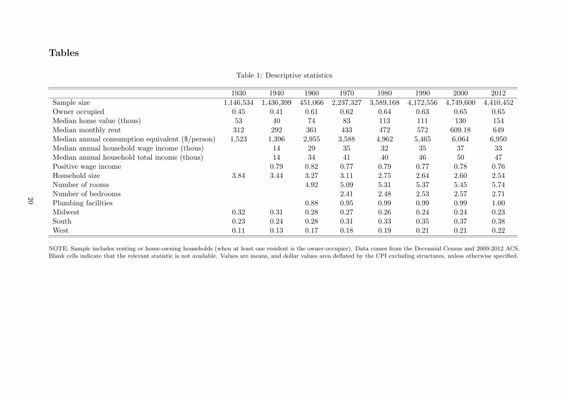
Table 1 provides basic characteristics of the sample. The first row shows how home-ownership

fell after the Great Depression and rose dramatically after World War II, hovering just above

60 percent for over fifty years. Household size consistently fell (from 3.8 in 1930, 3.3 in 1960,

to 2.5 in 2012) and the number of rooms per house rose slowly after 1960 (from 5 to 5.75)

along with the number of bedrooms. Indoor plumbing was common but not ubiquitous in 1960,

but became so by 1980. Taken together, these trends imply Americans consumed much more

housing per person. The fraction living in the South and West also ballooned from 35 to 60

percent, while the Midwest and Northeast lost its former predominance.

Figure 1 graphs Lorenz curves for various measures of housing outcomes and incomes in

1930, 1970, and 2012. We present Lorenz curves because they show how each part of the

distribution has changed over time.

Panel A shows that, among home-owners, 2012 and 1930 have almost identical levels of

inequality, with 50 percent of housing value accruing to the top 20 percent. Inequality is

uniformly lower in 1970 with 40 percent going to the top 20 percent. To better understand the

distribution of housing assets (if not equity) Panel B includes renters as zeroes. Here we see

1930 is considerably less equal, with 80 percent of owner-occupied housing wealth accruing to 20

percent of households, resembling the original “Pareto Principle,” for 19th-Century landowners.

In comparison, inequality in 2012 is much lower, although changes in the number of farms may

influence this number.

Panel C shows that rents were quite unequal in 1930, but that they were much more equal

in 1970. Since then, rent inequality has only grown slightly, primarily for costlier units. Panel

D shows consumption equivalents, which summarize much of the earlier discussion: 1930 had

the highest inequality, 1970 the least, and 2012 resembles 1930 at the top of the distribution

but 1970 at the bottom.

Panels E and F describe household wage income (not available in 1930) and total income

(not available in 1930 or 1940). Total income inequality is generally smaller, especially at the

bottom (partly due to lack of zeroes), and increased less than wage inequality between 1970

and 2012.

Figure 2 graphs our preferred inequality statistics in all years. Generally these show U-

6

shaped patterns from 1930 to 2012. Before 1970 there was a great compression in housing

consumption, similar to trends in the inequality of household income shown in Panel D.

From 1930 to 1970 the Theil entropy index and the variance of the log of home prices roughly

halved. Each statistic increases after 1970 — with a blip in 1990 that seems due to regional

housing booms — and settles in 2012 at a level slightly below its value in 1930. It is especially

remarkable that home-ownership waxed considerably during the great compression, while it did

not wane during the great divergence.

Rents exhibit a different pattern. While inequality in rents declined dramatically between

1930 and 1960, it increased less than home values in the period starting in 1980. Since inequality

changed more at the top than at the bottom, this may relate to increased levels of housing

assistance for low-income households, or rent control in major cities like New York and San

Francisco.

The consumption equivalent measure accounts for changes in demographics and home own-

ership, and exhibits a U-shaped pattern that is slightly less extreme in the latter half of the U.

This measure shows the lowest levels of inequality in 1980, while the other measures bottomed-

out closer to 1960. Inequality in consumption equivalents appears to be currently at its highest

level since World War II and seems to be increasing.

While we only have household wage income in 1940 (and nothing in 1930) it is worth noting

that inequality in our housing measures fell more between 1940 and 1960 than measures of

income. Subsequent increases in housing inequality since 1960 have been comparatively gentler.

3.2 Decomposition over Space

In Figure 3 and Table 3 we use a spatial decomposition to see how much inequality is due to

differences across areas as opposed to within them. Differences across cities are likely labor

market driven, since CZs are designed to resemble local labor markets. Differences within cities

are likely due to dwelling characteristics, local amenities, and commuting opportunities.

In all cases, within-area inequality is much larger than between-area inequality, such that

the within statistics are generally between three to ten times as large. The U-shaped patterns

observed at the national level for each measure are reflected both within and across states and

commuting zones. However, given the relative magnitudes, changes in inequality are mainly

driven by differences within metro areas. In contrast, much of the literature (examples include

Van Nieuwerburgh and Weill (2010), Diamond (2012), Gyourko, Mayer and Sinai (2013), and

7

Moretti (2013)) focuses on growing inequality between metro areas. Between-metro changes did

figure prominently in 1990 blip, which occurred in rents as well as prices, but have otherwise

been dwarfed by changes within metros.

The large increases in household wage inequality within areas in the late 20th century,

mirrors those in Baum-Snow and Pavan (2013), who find income inequality grew the most

within the largest U.S. cities. Meanwhile, inequality between metro areas declined considerably

between 1940 and 1960, and did not change considerably afterwards outside of the 1990 blip.

3.3 The Role of Observable Characteristics

Although the share of income devoted to housing appears to have stayed relatively constant

over the 20th century, patterns of housing consumption appears to have changed considerably.

As pointed out in Table 1, while households have shrunk in (human) size, their housing units

have gotten larger, and they have moved south and west.

Increases in housing price inequality since 1970 could be the result of two forces. First, some

households may have moved into ever larger units, while others moved into ever smaller units.

Second, Americans might have moved in ways that heightened inequality.

These hypotheses are examined in Figure 4 and Table 4. They show that if households lived

in housing units with dwelling characteristics, locations, and household composition observably

identical to those in 1970, housing values would be only slightly more equal. This accountable

change is very small in relation to the overall changes.15

The re-weighting results in Table 4 show that dwelling characteristics can explain at most

30 percent of the change in the two inequality statistics using the consumption equivalent

measure. The direction varies, however, with decreases in inequality among home owners and

increases for renters. Generally, changes in the location of houses and household composition

from 1970 to 2012 have tended to make households more equal in their housing outcomes. It is

also interesting, even surprising, that neither location nor dwelling characteristics do much to

explain changes in household wage inequality.

Our results on dwelling characteristics support previous reflections on this issue. For exam-

15The re-weighting specification we use allows for depreciation of housing by year at the cost of allowing for“vintage” effects of houses built in particular years. In an alternative specification we allow for these vintageeffects. Davis and Heathcote (2007) find that spending on structural improvements in the US (roughly 0.8percent) is very similar to a reasonable estimate of structural depreciation (roughly 1 percent). Our conclusionsusing vintages reinforce the idea that changes in dwelling characteristics have not driven the changes in housinginequality that we document.

8

ple, Glaeser and Gyourko (2008) find that per-capita square footage consumed by rich and poor

households has become more equal over time. Since construction costs vary little within cities,

much of the growing inequality in housing value seems to be due to growing inequality in land

values, or the right to build on such land.

3.4 The Relationship between Income and Housing Inequality

The patterns documented in section 3.2 suggest a link between local income and housing in-

equality. Studies of housing demand (e.g. Polinsky and Ellwood (1979), Hanushek and Quigley

(1980), and Mayo (1981)) have generally concluded that housing is a necessity, a regularity

sometimes known as “Schwabe’s Law.” Most estimates typically fall between 0.3 and 1.0. So

variations in income should be reflected in housing consumption. In fact, other things equal, the

variance of log housing consumption should equal the square of the income elasticity of housing

times the variance of log income.16

Patterns of income and housing inequality over time and space suggest a considerable re-

lationship between the two. For instance, between 1970 and 2012, the variance of log income

increased by 0.26, while the variance of log housing consumption increased by 0.09, consistent

with an income elasticity of 0.59.

We examine this relationship spatially in Figure 5 and Table 5 by comparing how inequality

within CZs for housing relate to income. Here we see that the two inequalities are strongly

related, and share a relationship of roughly the same magnitude. Column three of Table 5 takes

the square root of a regression of the variance of the logs of measure of housing consumption

on the variance of logs of household income. This produces estimates of the income elasticity

of housing expenditures in the range of 0.7 to 0.9, which are reasonable, if slightly higher than

values from temporal variation.

4 Conclusion

Our results provide some refinements to the debate on inequality, particularly in terms of

consumption and wealth. The similarity of housing and income inequality over space and time

according to plausible income elasticities appears to support those arguing that consumption

16This exercise carries several caveats: General equilibrium effects may interact with consumer preferences toeither dampen (Matlack and Vigdor (2008)) or amplify (Van Nieuwerburgh and Weill (2010)) the direct effects ofchanges in incomes. Additionally, since housing is so heterogeneous, it is difficult to quantify how much “housingservice” a house of a given size or in a given neighborhood provide.

9

inequality does reflect income inequality. Additionally, changes in dwelling characteristics and

differences between cities explain only a small fraction of recent increases in housing inequality.

This suggests that the value of land plays an important role, even within cities.17

Several studies — e.g., Green, Malpezzi and Mayo (2005), Gyourko, Saiz and Summers

(2008), and Saiz (2010) — have emphasized that regulatory and geographic constraints on

housing supply may play an important role in price differences across cities. Our findings suggest

constraints may play a role within cities, as new housing in the most desirable neighborhoods

may be the most constrained. These may interact with findings by Rossi-Hansberg, PierreDaniel

Sarte and Owens (2010), Guerrieri, Hartley and Hurst (2013), and Autor, Palmer and Pathak

(2014) on how local externalities that can lead to substantial income sorting within cities.

Generally, our findings suggest that researchers would do well to more closely examine differences

in land prices across neighborhoods. An interesting research project would be to determine how

much they are driven by local externalities, dwelling characteristics, and fixed neighborhood

amenities.

The growing inequality in housing prices that we document also indirectly supports findings

that wealth inequality has increased. High home-ownership levels do imply that inequality

in housing wealth is still smaller than it was in 1930. Nevertheless, the windfall gains from

unequal housing price changes, which benefited some homeowners relative to others, may help

stir once-popular Georgeist concerns about unequal land-ownership from the beginning of the

20th Century. Moreover, it appears that housing inequality will continue to grow in line with

any further increases in income inequality.

17Our result also supports findings by Watson (2009) and Reardon and Bischoff (2011) that segregation byincome has increased since 1970. This contrasts with findings by Glaeser and Vigdor (2012) and others thatblack-white segregation peaked in 1970 and has since declined.

10

References

Aguiar, Mark A, and Mark Bils. 2011. “Has Consumption Inequality Mirrored Income

Inequality?” National Bureau of Economic Research.

Albouy, David, and Bert Lue. 2015. “Driving to opportunity: Local rents, wages,

commuting, and sub-metropolitan quality of life.” Journal of Urban Economics, 89: 74–92.

Atkinson, Anthony B. 1970. “On the measurement of inequality.” Journal of Economic

Theory, 2: 244–263.

Atkinson, Anthony B, Thomas Piketty, and Emmanuel Saez. 2011. “Top Incomes

in the Long Run of History.” Journal of Economic Literature, 49(1): 3–71.

Attanasio, Orazio P., and Luigi Pistaferri. 2014. “Consumption inequality over the

last half century: Some evidence using the new PSID consumption measure.” American

Economic Review, 104(5): 122–126.

Autor, David H., Christopher J. Palmer, and Parag A. Pathak. 2014. “Housing

Market Spillovers: Evidence from the End of Rent Control in Cambridge, Massachusetts.”

Journal of Political Economy, 122(3): 661–717.

Autor, David H., David Dorn, and Gordon Hanson. 2013. “The China Syndrome:

Local Labor Market Effects of Import Competition in the United States.” American

economic Review, 103(6): 2121–2168.

Baum-Snow, Nathaniel, and Ronni Pavan. 2013. “Inequality and City Size.” Review

of Economics and Statistics, 95(5): 1535–1548.

Bonnet, Odran, Pierre-Henri Bono, Guillaume Chapelle, and Etienne Wasmer.

2014. “Does housing capital contribute to inequality? A comment on Thomas Pikettys

Capital in the 21st Century.” Sciences Po Economics Discussion Papers, 7.

Chao, Elaine L., and Kathleen P. Utgoff. 2006. “100 Years of US Consumer Spending

Data for the Nation, New York City, and Boston.” United States Department of Labor 991.

Cowell, Frank. 2011. Measuring inequality. Oxford University Press.

Cutler, David M., and L. F. Katz. 1992. “Rising inequality? Changes in the

distribution of income and consumption in the 1980’s.” American Economic Review,

82(2): 546–551.

Davis, Morris A., and Jonathan Heathcote. 2007. “The price and quantity of

residential land in the United States.” Journal of Monetary Economics, 54(8): 2595–2620.

11

Diamond, Rebecca. 2012. “The Determinants and Welfare Implications of US Workers

Diverging Location Choices by Skill: 1980-2000.” Unpublished Manuscript, Harvard

University.

DiNardo, John, Nicole M Fortin, and Thomas Lemieux. 1996. “Labor Market

Institutions and the Distribution of Wages, 1973-1992: A Semiparametric Approach.”

Econometrica, 64(5): 1001–1044.

Dorn, David. 2009. “Essays on Inequality, Spatial Interaction, and the Demand for

Skills.” PhD diss.

Firpo, Sergio. 2007. “Efficient semiparametric estimation of quantile treatment effects.”

Econometrica, 75(1): 259–276.

Fortin, Nicole, Thomas Lemieux, and Sergio Firpo. 2011. “Chapter 1

Decomposition Methods in Economics.” In Handbook of Labor Economics. Vol. 4, 1–102.

Friedman, Milton. 1957. A theory of the consumption function. Princeton:Princeton

University Press.

Glaeser, Edward, and Jacob Vigdor. 2012.

The end of the segregated century: racial separation in America’s neighborhoods, 1890-2010.

Manhattan Institute for Policy Research New York, NY.

Glaeser, E.L., and J.E. Gyourko. 2008.

Rethinking federal housing policy: how to make housing plentiful and affordable. Vol. 76.

Goldin, Claudia, and Robert A. Margo. 1992. “The Great Compression: The Wage

Structure in the United States at Mid- Century.” The Quarterly Journal of Economics,

107(1): 1–34.

Green, Richard K., Stephen Malpezzi, and Stephen K. Mayo. 2005.

“Metropolitan-specific estimates of the price elasticity of supply of housing, and their

sources.”

Guerrieri, Veronica, Daniel Hartley, and Erik Hurst. 2013. “Endogenous

gentrification and housing price dynamics.” Journal of Public Economics, 100: 45–60.

Gyourko, Joseph, Albert Saiz, and Anita Summers. 2008. “A new measure of the

local regulatory environment for housing markets: The Wharton Residential Land Use

Regulatory Index.” Urban Studies, 45(3): 693–729.

Gyourko, Joseph, Christopher Mayer, and Todd Sinai. 2013. “Superstar Cities.”

American Economic Journal: Economic Policy, 5(4): 167–199.

12

Hanushek, Eric A, and John M Quigley. 1980. “What is the Price Elasticity of

Housing Demand?” Source: The Review of Economics and Statistics, 62(3): 449–454.

Hirano, Keisuke, Guido W. Imbens, and Geert Ridder. 2003. “Efficient Estimation

of Average Treatment Effects Using the Estimated Propensity Score.”

Kopczuk, Wojciech. 2004. “Top Wealth Shares in the United States, 1916- 2000:

Evidence from Estate Tax Returns.”

Kopczuk, Wojciech. 2015. “What Do We Know about the Evolution of Top Wealth

Shares in the United States?” Journal of Economic Perspectives, 29(1): 47–66.

Krueger, Dirk, and Fabrizio Perri. 2006. “Does income inequality lead to consumption

inequality? Evidence and theory.” Review of Economic Studies, 73(1): 163–193.

Matlack, Janna L., and Jacob L. Vigdor. 2008. “Do rising tides lift all prices? Income

inequality and housing affordability.” Journal of Housing Economics, 17(3): 212–224.

Mayo, Stephen K. 1981. “Theory and estimation in the economics of housing demand.”

Journal of Urban Economics, 10(1): 95–116.

Meyer, Bruce, and James Sullivan. 2010. “Consumption and Income Inequality in the

US Since the 1960s.” University of Chicago manuscript.

Moretti, Enrico. 2013. “Real wage inequality.” American Economic Journal: Applied

Economics, 5(1): 65–103.

Peiser, Richard B., and Lawrence B. Smith. 1985. “Homeownership Returns, Tenure

Choice and Inflation.” Real Estate Economics, 13: 343–360.

Piketty, Thomas, and Emmanuel Saez. 2003. “Income Inequality in the United States,

1913–1998.” The Quarterly Journal of Economics, 118(February): 1–39.

Piketty, Thomas, and Gabriel Zucman. 2014. “Capital is back: Wealth-income ratios

in rich countries, 1700-2010.” The Quarterly Journal of Economics.

Polinsky, A Mitchell, and David T Ellwood. 1979. “An empirical reconciliation of

micro and grouped estimates of the demand for housing.” The Review of Economics and

Statistics, 199–205.

Poterba, James, and Todd Sinai. 2008. “Tax Expenditures for Owner-Occupied

Housing: Deductions for Property Taxes and Mortgage Interest and the Exclusion of

Imputed Rental Income.” American Economic Review, 98(2): 84–89.

Reardon, Sean F, and Kendra Bischoff. 2011. “Income inequality and income

segregation.” American Journal of Sociology, 116(4): 1092–1153.

13

Rognlie, Matthew. 2014. “A note on Piketty and diminishing returns to capital.”

Rossi-Hansberg, Esteban, PierreDaniel Sarte, and Raymond Owens. 2010.

“Housing Externalities.” Journal of Political Economy, 118(3): pp. 485–535.

Ruggles, Steven, J. Trent Alexander, Katie Genadek, Ronald Goeken,

Matthew B. Schroeder, and Matthew Sobek. 2010. “Integrated Public Use Microdata

Series: Version 5.0.”

Saez, Emmanuel, and Gabriel Zucman. 2014. “Wealth Inequality in the United States

since 1913: Evidence from Capitalized Income Tax Data.” National Bureau of Economic

Research Working Paper Series, No. 20625.

Saiz, A. 2010. “The geographic determinants of housing supply.” The Quarterly Journal of

Economics, 125(3).

Tolbert, Charles M., and Molly Sizer. 1996. “U.S. Commuting Zones and Labor

Market Areas: A 1990 Update.”

Van Nieuwerburgh, Stijn, and Pierre-Olivier Weill. 2010. “Why Has House Price

Dispersion Gone Up?” Review of Economic Studies, 77(4): 1567–1606.

Verbrugge, Randal. 2008. “The puzzling divergence of rents and user costs, 1980-2004.”

Review of Income and Wealth, 54(4): 671–699.

Watson, Tara. 2009. “Inequality and the measurement of residential segregation by

income in american neighborhoods.” Review of Income and Wealth, 55(3): 820–844.

14

Figures

Figure 1: Lorenz Curves for Home Values, Rents, Housing Consumption, and Household Income

0.2

.4.6

.81

Cum

ula

tive

dis

trib

uti

on

0 .2 .4 .6 .8 1Cumulative population proportion

Panel A: Home values

0.2

.4.6

.81

Cum

ula

tive

dis

trib

uti

on


Panel B: Home values (0 for renters)

0.2

.4.6

.81

Cum

ula

tive

dis

trib

uti

on


Panel C: Rents

0.2

.4.6

.81

Cum

ula

tive

dis

trib

uti

on


Panel D: Consumption equivalent

0.2

.4.6

.81

Cum

ula

tive

dis

trib

uti

on


Panel E: Household wage income

0.2

.4.6

.81

Cum

ula

tive

dis

trib

uti

on


Panel F: Household total income

1930 1970 2012

NOTE: These curves graph the cumulative percentage of housing expenditures (from lowest to highest), against the cumulative percentage of

households. Panel A, is for owning households; Panel C is for renters. All others are for the sample of home owners and renters combined. Panel B

includes renters with an implied home value of zero. Data are interpolated within intervals as described in the text. Data are from the Decennial

Census and the 2009-2012 ACS. See the text and data appendix for more detail.

15

Figure 2: Inequality over Time in Home Values, Rents, Housing Consumption, and HouseholdIncome

0.1

.2.3

.4.5

.6In

dex

(G

ini

and

Thei

l)

0.5

11

.5L

og

do

llar

s (V

ar o

f lo

gs)

1930

1940

1960

1970

1980

1990

2000

2012


0.1

.2.3

.4.5

.6In

dex

(G

ini

and

Thei

l)

0.5

11

.5L

og

do

llar

s (V

ar o

f lo

gs)

1930

1940

1960

1970

1980

1990

2000

2012

Panel B: Rents

0.1

.2.3

.4.5

.6In

dex

(G

ini

and

Th

eil)

0.5

11

.5L

og

do

llar

s (V

ar o

f lo

gs)

1930

1940

1960

1970

1980

1990

2000

2012

Panel C: Consumption equivalent

0.1

.2.3

.4.5

.6In

dex

(G

ini

and

Th

eil)

0.5

11

.5L

og

do

llar

s (V

ar o

f lo

gs)

1930

1940

1960

1970

1980

1990

2000

2012

Panel D: Household wage income

Var of Logs Theil entropy Gini

NOTE: Each presents inequality measures for separate samples. The first is for home owners and is the dollar

value of their primary residence. The second is for renters and is their cash expenditure per month on rent and

utilities. The final combines the two to compute an consumption measure per person, as explained in the text.

Farms and houses used for business are excluded. Data are interpolated within intervals. The observation for

2012 comes from ACS for 2009-2012. See text and Data Appendix for more detail.

16

Figure 3: Decomposition of Values Between and Across Geographies.

Panel A: Theil entropy

0.0

5.1

.15

.2.2

5B

etw

een v

alue

0.1

.2.3

.4W

ithin

val

ue

1930

1940

1960

1970

1980

1990

2000

2012


0.0

5.1

.15

.2.2

5B

etw

een v

alue

0.1

.2.3

.4W

ithin

val

ue

1930

1940

1960

1970

1980

1990

2000

2012

Panel B: Rents

0.0

5.1

.15

.2.2

5B

etw

een v

alue

0.1

.2.3

.4W

ithin

val

ue

1930

1940

1960

1970

1980

1990

2000

2012


0.0

5.1

.15

.2.2

5B

etw

een v

alue

0.1

.2.3

.4W

ithin

val

ue

1930

1940

1960

1970

1980

1990

2000

2012


Between CZ Between State

Within CZ Within State

Panel B: Variance of logs

0.0

5.1

.15

.2.2

5B

etw

een v

alue

0.2

5.5

.75

1W

ithin

val

ue

1930

1940

1960

1970

1980

1990

2000

2012


0.0

5.1

.15

.2.2

5B

etw

een v

alue

0.2

5.5

.75

1W

ithin

val

ue

1930

1940

1960

1970

1980

1990

2000

2012

Panel B: Rents

0.0

5.1

.15

.2.2

5B

etw

een v

alue

0.2

5.5

.75

1W

ithin

val

ue

1930

1940

1960

1970

1980

1990

2000

2012


0.0

5.1

.15

.2.2

5B

etw

een v

alue

0.2

5.5

.75

1W

ithin

val

ue

1930

1940

1960

1970

1980

1990

2000

2012


Between CZ Between State

Within CZ Within State

NOTE: Between and within decompositions of housing expenditures are shown for the Theil entropy index and

the variance of logarithms. See earlier figure nots for details about the sample.

17

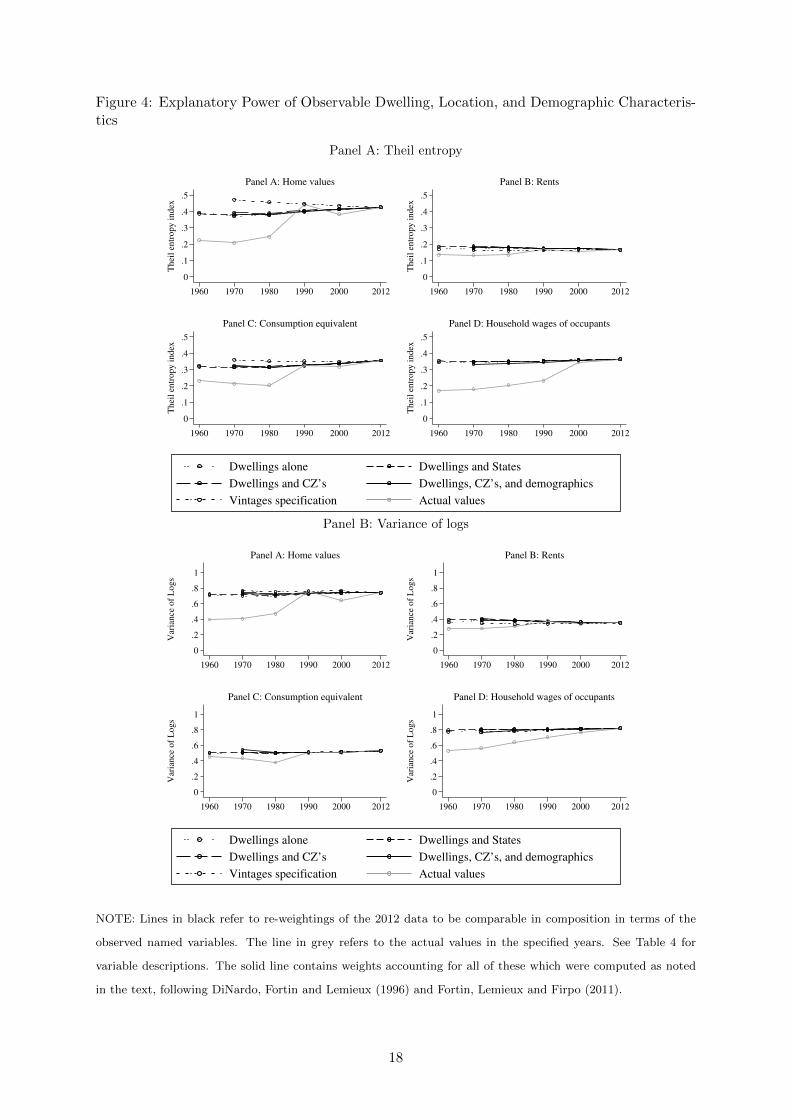
Figure 4: Explanatory Power of Observable Dwelling, Location, and Demographic Characteris-tics


0

.1

.2

.3

.4

.5

Thei

l en

tropy i

ndex

1960 1970 1980 1990 2000 2012


0

.1

.2

.3

.4

.5

Thei

l en

tropy i

ndex

1960 1970 1980 1990 2000 2012

Panel B: Rents

0

.1

.2

.3

.4

.5

Thei

l en

tropy i

ndex

1960 1970 1980 1990 2000 2012


0

.1

.2

.3

.4

.5

Thei

l en

tropy i

ndex

1960 1970 1980 1990 2000 2012

Panel D: Household wages of occupants

Dwellings alone Dwellings and States

Dwellings and CZ’s Dwellings, CZ’s, and demographics

Vintages specification Actual values


0

.2

.4

.6

.8

1

Var

iance

of

Logs

1960 1970 1980 1990 2000 2012


0

.2

.4

.6

.8

1

Var

iance

of

Logs

1960 1970 1980 1990 2000 2012

Panel B: Rents

0

.2

.4

.6

.8

1

Var

iance

of

Logs

1960 1970 1980 1990 2000 2012


0

.2

.4

.6

.8

1

Var

iance

of

Logs

1960 1970 1980 1990 2000 2012

Panel D: Household wages of occupants

Dwellings alone Dwellings and States

Dwellings and CZ’s Dwellings, CZ’s, and demographics

Vintages specification Actual values

NOTE: Lines in black refer to re-weightings of the 2012 data to be comparable in composition in terms of the

observed named variables. The line in grey refers to the actual values in the specified years. See Table 4 for

variable descriptions. The solid line contains weights accounting for all of these which were computed as noted

in the text, following DiNardo, Fortin and Lemieux (1996) and Fortin, Lemieux and Firpo (2011).

18

Figure 5: Local Inequality in Housing versus Income

Panel A: Home value inequality.2

.4.6

.81

Var

ian

ce o

f lo

gs

of

ho

me

val

ues

.5 .6 .7 .8 .9 1

Variance of logs of household total incomeLine slope: 0.019 (0.045) R−squared: 0.000

Panel B: Rent inequality

.1.2

.3.4

Var

ian

ce o

f lo

gs

of

ren

ts

.5 .6 .7 .8 .9 1

Variance of logs of household total incomeLine slope: 0.392 (0.019) R−squared: 0.383

Panel C: Consumption equivalent inequality

.2.4

.6.8

Var

iance

of

logs

of

consu

mpti

on e

quiv

alen

t

.5 .6 .7 .8 .9 1Variance of logs of household total income

Line slope: 0.743 (0.035) R−squared: 0.387

NOTE: These panels display scatter plots for commuting zones with the variance of logs of total income recorded

in the 2009-2012 ACS on the x axis and each measure of housing expenditure inequality on the y axis (with zeros

excluded). Each variable is computed for its relevant population with the variance of the logs of household total

income including both owners and renters in each graph. The size of each circle is proportionate to the number

of (weighted) households in each commuting zone. The OLS regression line plotted incorporate these weights.

19

Tables

Table 1: Descriptive statistics

1930 1940 1960 1970 1980 1990 2000 2012

Sample size 1,146,534 1,436,399 451,066 2,237,327 3,589,168 4,172,556 4,749,600 4,410,452Owner occupied 0.45 0.41 0.61 0.62 0.64 0.63 0.65 0.65Median home value (thous) 53 40 74 83 113 111 130 154Median monthly rent 312 292 361 433 472 572 609.18 649Median annual consumption equivalent ($/person) 1,523 1,396 2,955 3,588 4,962 5,465 6,064 6,950Median annual household wage income (thous) 14 29 35 32 35 37 33Median annual household total income (thous) 14 34 41 40 46 50 47Positive wage income 0.79 0.82 0.77 0.79 0.77 0.78 0.76Household size 3.84 3.44 3.27 3.11 2.75 2.64 2.60 2.54Number of rooms 4.92 5.09 5.31 5.37 5.45 5.74Number of bedrooms 2.41 2.48 2.53 2.57 2.71Plumbing facilities 0.88 0.95 0.99 0.99 0.99 1.00Midwest 0.32 0.31 0.28 0.27 0.26 0.24 0.24 0.23South 0.23 0.24 0.28 0.31 0.33 0.35 0.37 0.38West 0.11 0.13 0.17 0.18 0.19 0.21 0.21 0.22

NOTE: Sample includes renting or home-owning households (when at least one resident is the owner-occupier). Data comes from the Decennial Census and 2009-2012 ACS.Blank cells indicate that the relevant statistic is not available. Values are means, and dollar values area deflated by the CPI excluding structures, unless otherwise specified.

20

Table 2: Inequality statistics

Home Values 1930 1970 2012

Variance of logs 0.823 0.402 0.739

Theil entropy 0.443 0.210 0.426

Gini coefficient 0.468 0.341 0.462

Ratio of 90 to 10th percentiles 11.159 5.399 9.295

Rent


Theil entropy 0.319 0.132 0.167



Consumption equivalent


Theil entropy 0.434 0.213 0.355



Household wage income 1940 1970 2012


Theil entropy 0.227 0.181 0.362


Ratio of 90 to 10th percentiles

NOTE: Home values refer to owner-occupied homes. Rents are gross and include the cost of utilities. Both are

self reported. Consumption equivalents combine gross rents with imputed rents based on a percentage of the

home value plus utility costs, divided by the equivalence scale 1 + 0.7(A − 1) + 0.5C where A is the number of

adults and C is the number of children under 14. Household wage income refers is the sum of wages and salaries

from all household members. Values are interpolated within intervals using standard procedures described in the

text.

21

Table 3: Between-Within decomposition

Panel A: Home Values

1930 1970 2012

Variance Overall 0.823 0.403 0.746

Variance Between 0.215 0.097 0.208

Variance Within 0.607 0.306 0.538

Theil Overall 0.443 0.210 0.426

Theil Between 0.084 0.042 0.115

Theil Within 0.359 0.168 0.311

Panel B: Rents

1930 1970 2012




Theil Overall 0.318 0.132 0.167

Theil Between 0.076 0.026 0.044

Theil Within 0.242 0.106 0.122

Panel C: Consumption equivalents

1930 1970 2012




Theil Overall 0.434 0.213 0.355

Theil Between 0.068 0.024 0.049

Theil Within 0.366 0.189 0.306


1940 1970 2012




Theil Overall 0.227 0.179 0.362

Theil Between 0.021 0.009 0.019

Theil Within 0.205 0.170 0.343

NOTE: Between and within decompositions refer to the decomposition of each statistics to variation within states

or commuting zones (CZs) versus between them. The sum corresponds to values in table 2.

22

Table 4: Re-weighting


Consumption equiv Rents Home values HH wages

2012 0.355 0.167 0.426 0.362

Dwellings 0.315 0.176 0.371 0.344

Dwellings and state 0.312 0.182 0.378 0.347

Dwellings and CZ 0.317 0.187 0.392 0.350

Dwellings, CZ, and demographics 0.325 0.177 0.385 0.333

1970 0.213 0.132 0.210 0.181


Consumption equiv Rents Home values HH wages

2012 0.527 0.351 0.739 0.820

Dwellings 0.505 0.383 0.698 0.796

Dwellings and state 0.503 0.394 0.716 0.800

Dwellings and CZ 0.510 0.404 0.746 0.806

Dwellings, CZ, and demographics 0.541 0.388 0.733 0.768

1970 0.437 0.279 0.402 0.563

NOTE: Statistics are taken of 2012 data, re-weighted to emulate the distribution of observable dwelling and

location characteristics of previous years. The top and bottom row refers to the actual values in the specified years.

Dwellings refers to: Indicators for the number of rooms, bedrooms, the decade of construction, plumbing facilities,

and the heating system type. States and CZs include indicators for the geographic entities, and demographics is

the interactions of the household type (single, a couple, a single parent, or non-related individuals) with indicators

for the number of children and adults (separately). The solid line contains weights accounting for all of these

which were computed as noted in the text, following DiNardo, Fortin and Lemieux (1996) and Fortin, Lemieux

and Firpo (2011).

23

Table 5: Implied relationships with income inequality

Home values Rents Consumption equivalent

1970 0.720 0.629 0.755

(0.133) (0.048) (0.054)

1980 0.764 0.690 0.715

(0.157) (0.072) (0.039)

1990 0.365 0.654 0.782

(0.167) (0.031) (0.128)

2000 0.444 0.620 0.789

(0.124) (0.037) (0.074)

2012 0.138 0.626 0.862

(0.568) (0.057) (0.094)

NOTE: Each coefficient is the (re-signed) square root of the absolute value of the regression coefficient relating

the variance of the log of household wage income within each CZ with the variance of the log of the variable within

each CZ. Standard errors clustered by the state the plurality of the CZ’s population lives in are in parenthesis.

The unit of observation for each regression is a CZ year and each coefficients is from a different regression. Each

is computed using the relevant sample for that variable while income inequality is computed using the universe

of all home owners and renters. The third column represents an estimate of the income elasticity of demand for

housing services. See tables 1 and 2 and figure 5 for more detail.

24

Appendix - For Online Publication

A Data appendix

A.1 Integrated Public Use Microdata Series samples

Our Census data are provided by the Integrated Public Use Microdata Series, from usa.ipums.orgdetailed in Ruggles et al. (2010). For each year we use the following samples.

• 1930: 5 percent sample


• 1960: 1 percent

• 1970: 1 percent state and metro (depending on state or commuting zone) and format 1or 2 (depending on the questions needed).

• 1980: 5 percent state sample



• 2009-12 ACS five year 2012 sample with interviews in 2008 dropped

A.2 Sample restrictions

As mentioned in the main text, we include households in the United States with three restric-tions: We omit houses outside the continental US, we exclude houses used to generate revenue,and we similarly exclude owner occupied multiple family residences. Appendix table A.1 showsthe percentage of houses we exclude for each year due to being used to generate revenue orencompassing multiple units. We present these separately for both owners and renters.

The first row for each panel shows the number of houses in the continental US that areincluded in our sample. this is quite high for each year, and in later years it is over 90 percent.The next few rows show reasons why houses are excluded. By far the most important reason isbecause they are farms. For example, in 1930 25 percent of households lived on a farm. Multiplefamily houses and houses used for commercial purposes are also excluded in our analysis forthe years where the census identifies them. In 1960, the first year we can identify them, thesehousing categories made up roughly 6 percent of owner occupied housing.

The final few rows show categories of houses that were excluded from questions in someyears. From 1960-1980 mobile homes and trailers were excluded and in 1970 condos were aswell. In other years they are included. These categories, again, make up a small proportion ofhousing units in these years, They never reach six percent, and often are well below that mark.

i

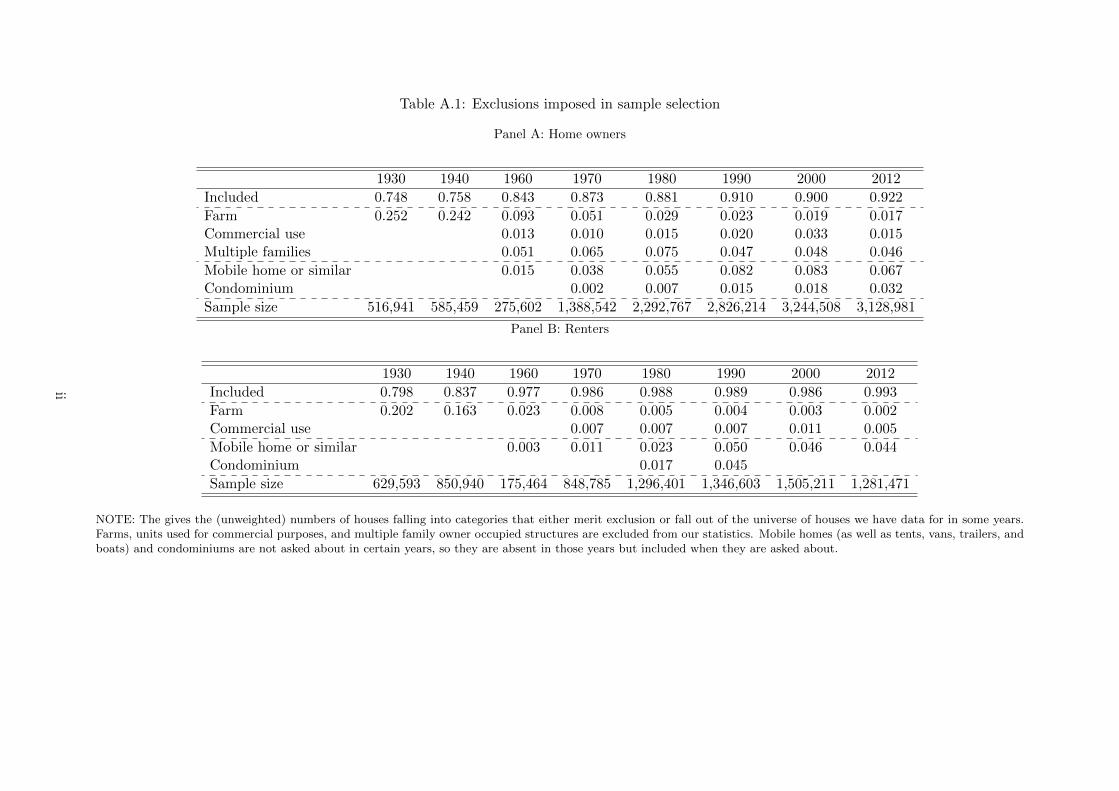
Table A.1: Exclusions imposed in sample selection

Panel A: Home owners

1930 1940 1960 1970 1980 1990 2000 2012

Included 0.748 0.758 0.843 0.873 0.881 0.910 0.900 0.922

Farm 0.252 0.242 0.093 0.051 0.029 0.023 0.019 0.017Commercial use 0.013 0.010 0.015 0.020 0.033 0.015Multiple families 0.051 0.065 0.075 0.047 0.048 0.046

Mobile home or similar 0.015 0.038 0.055 0.082 0.083 0.067Condominium 0.002 0.007 0.015 0.018 0.032

Sample size 516,941 585,459 275,602 1,388,542 2,292,767 2,826,214 3,244,508 3,128,981

Panel B: Renters

1930 1940 1960 1970 1980 1990 2000 2012

Included 0.798 0.837 0.977 0.986 0.988 0.989 0.986 0.993

Farm 0.202 0.163 0.023 0.008 0.005 0.004 0.003 0.002Commercial use 0.007 0.007 0.007 0.011 0.005

Mobile home or similar 0.003 0.011 0.023 0.050 0.046 0.044Condominium 0.017 0.045

Sample size 629,593 850,940 175,464 848,785 1,296,401 1,346,603 1,505,211 1,281,471

NOTE: The gives the (unweighted) numbers of houses falling into categories that either merit exclusion or fall out of the universe of houses we have data for in some years.Farms, units used for commercial purposes, and multiple family owner occupied structures are excluded from our statistics. Mobile homes (as well as tents, vans, trailers, andboats) and condominiums are not asked about in certain years, so they are absent in those years but included when they are asked about.

ii

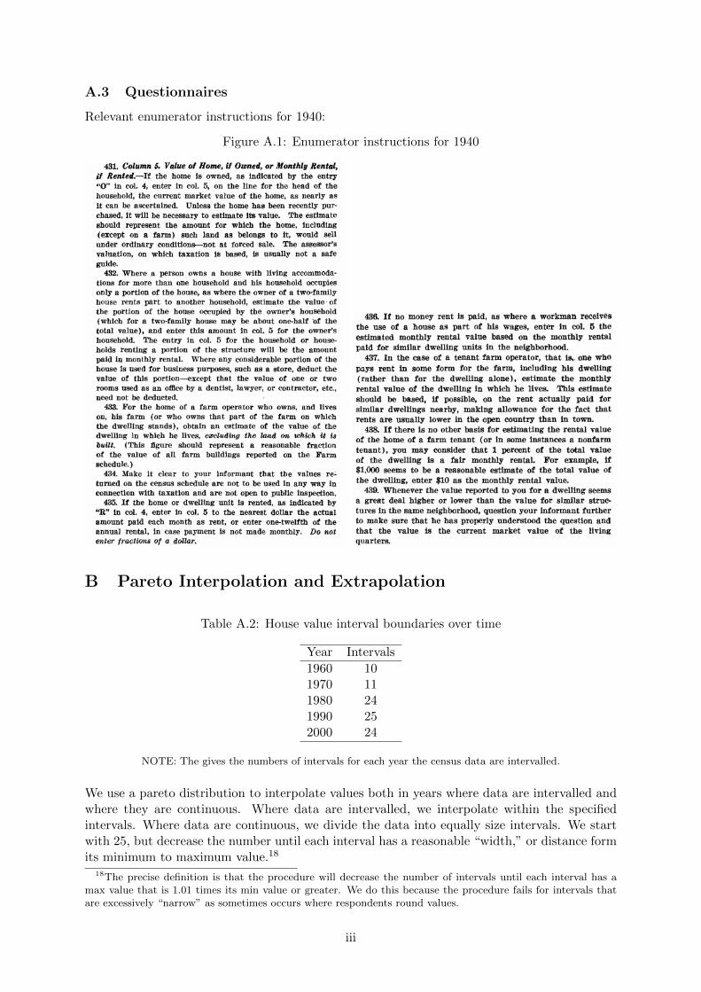
A.3 Questionnaires

Relevant enumerator instructions for 1940:

Figure A.1: Enumerator instructions for 1940

B Pareto Interpolation and Extrapolation

Table A.2: House value interval boundaries over time

Year Intervals

1960 101970 111980 241990 252000 24

NOTE: The gives the numbers of intervals for each year the census data are intervalled.

We use a pareto distribution to interpolate values both in years where data are intervalled andwhere they are continuous. Where data are intervalled, we interpolate within the specifiedintervals. Where data are continuous, we divide the data into equally size intervals. We startwith 25, but decrease the number until each interval has a reasonable “width,” or distance formits minimum to maximum value.18

18The precise definition is that the procedure will decrease the number of intervals until each interval has amax value that is 1.01 times its min value or greater. We do this because the procedure fails for intervals thatare excessively “narrow” as sometimes occurs where respondents round values.

iii

The pareto distribution’s cumulative distriubtuion function (CDF) has the from F (y) =1−(k/y)α for y ≥ k. It follows that the logarithm of the complementary CDF (or “tail” function)has a slope of −α with respect to ln(y). The greater the slope α, the faster observations “dieoff,” and the less disperse the distribution. For any value yi, define

pi ≡ ln[1− F (y)] = α ln(k)− α ln(y) (A.1)

The interpolation method (Pareto (1896)) estimates α by differencing expression A.1 at thevalues for the two endpoints of a bracket [yi, yi+1], where i = 1, ..., I indexes the intervals,namely

αi =ln(yi+1)− ln(yi)

pi − pi+1, i = 1, ..., I − 1, (A.2)

and ki = yip1/αi . Even when the distribution may not be considered Pareto globally, this

procedure fits a simple line segment to the log survivor function in terms of ln(y).Since the Pareto distribution is unbounded, determining a value of α beyond the top code,

yI in the data can be difficult. This problem is largely remedied if the mean is available, asit is for housing values in 1930, 1940, and 2012. There, the property that the mean value ofyI ≡ E[y|y ≥ yI ] = αyI/(α− 1), imples a value of

αI =yI

yI − yI(A.3)

In other situations it is impossible to obtain a mean above a given cutoff. In these cases weinfer a value of α by taking the average of values from the linear interpolation method (A.2)for the top 10 percent of the distribution that do not correspond to the top interval.19For rentvalues in 1930 and 1940, we code the top pareto parameter to be 2.5, which roughly correspondsto this.

For the bottom-most interval we employ a simple strategy of imposing a uniform distribu-tion so our choices impact our results as minimally as possible. To do this we need to establisha minimum possible value for the variable we are concerned with. The bottom value is deter-mined to be, for rents, 0.03 percent of average household incomes per year (corresponding to ahousehold that makes 10 percent of the average household income and spends 1/3 of it on rent).For home values it is the same value, but divided by 0.0785, which is the rent to value ratiowe use to convert housing values into user costs of housing. For household incomes it is the 0.1times average household income in that year. Average (national) household incomes for thispurpose across the many years in our sample come from Chao and Utgoff (2006). How we treatbottom values matters little except for in the variance of logarithms, which has undesirableproperties at the bottom of the distribution (for instance, it cannot account for zero values).

Figure A.2 shows several illustrations of our imputation procedure for different types ofsituations. We plot both the CDF and the tail function, which is linear in the pareto distribution.The second plot is especially relevant for determining the fit in the very top of the distribution.

Panel A of Figure A.2 shows both the empirical cumulative density function for home pricesin 2012 and the pareto CDF used in the paper. Note that this is a year where respondentsreported a continuous quantity, though the distribution plot shows that many did round. Thedashed lines show intervals in each bin used for rounding. As in other years, we divided thedata into 25 bins to perform the CDF interpolation. The dashed lines show the min and maxproportions for each bin, as well as its placement along the scale.

Figure Panel B, which shows a plot of the tail function, which shows how the Pareto distri-

19In the extremely rare case where all values in the top 10 percent are in the top bin, we check the top 11, 12,13, etc. percent, stopping at the first percentile where an estimate exists.

iv

bution matches the top of the distribution. Overall the fit is quite good, with the line trackingthe distribution until it encounters the state by year topcodes for the top 0.5 percent of thedistribution.

Similarly Panel C and Panel D show the same for the 1970 distribution where the variableis divided into 11 intervals. Here the distribution meets the interval boundaries exactly and theinterpolation simply smooths the area between them. The top code extrapolation has the sameslope as the one for 2012, but this slope matches the slope of the previous interval rather well,implying the extrapolation is reasonable for this year as well.

Figure A.2: Example CDF plots for the pareto interpolation

Panel A: CDF of house values for 2012

0.2

.4.6

.81

25

,06

9

40

,00

0

57

,00

0

70

,00

0

80

,00

0

90

,00

01

00

,00

0

11

5,0

00

12

5,0

00

14

0,0

00

15

0,0

00

16

0,0

00

17

5,0

00

19

0,0

00

20

0,0

00

22

5,0

00

25

0,0

00

27

0,0

00

30

0,0

00

33

0,0

00

38

0,0

00

45

0,0

00

55

0,0

00

75

0,0

00

CDF with ties Proportion below lower bound

Proportion below upper bound CDF of interpolation

Panel B: Tail function of house values for 2012

−1

5−

10

−5

0

25

,06

9

40

,00

0

57

,00

0

70

,00

0

80

,00

0

90

,00

01

00

,00

0

11

5,0

00

12

5,0

00

14

0,0

00

15

0,0

00

16

0,0

00

17

5,0

00

19

0,0

00

20

0,0

00

22

5,0

00

25

0,0

00

27

0,0

00

30

0,0

00

33

0,0

00

38

0,0

00

45

0,0

00

55

0,0

00

75

0,0

00

Log of one minus smooth CDF ln(1−Fmin)

ln(1−Fmax) Transformed CDF of Interpolation

Panel C: CDF of house values for 1970

0.2

.4.6

.81

4,0

63

5,0

00

7,5

00

10

,00

0

12

,50

0

15

,00

0

17

,50

0

20

,00

0

25

,00

0

35

,00

0

50

,00

0

CDF with ties Proportion below lower bound

Proportion below upper bound CDF of interpolation

Panel D: Tail function of house values for 1970

−1

5−

10

−5

0

4,0

63

5,0

00

7,5

00

10

,00

0

12

,50

0

15

,00

0

17

,50

0

20

,00

0

25

,00

0

35

,00

0

50

,00

0

Log of one minus smooth CDF ln(1−Fmin)

ln(1−Fmax) Transformed CDF of Interpolation

NOTE: The term “tail function” corresponds to the logarithm of one minus the the CDF.

C Geographic Assignment

We keep a consistent geographic sample across all years in the sample by primarily using 1990local labor markets, or commuting zones, as described by Tolbert and Sizer (1996). Local labormarkets are a natural geography for this analysis since housing values are closely related to localincome levels. For 1970-2011 we match geographically using the probabilistic mapping madeavailable by David Dorn via his website and used in, for example, Dorn (2009). For 2012 wereplicate the probabalistis matching using updated PUMA definitions for the 2012 census andfor 1930 and 1940 we use the direct county to commuting zone mapping in Tolbert and Sizer

v

(1996) since counties are available. Unfortunately it is not possible to match to commuing zonesin for 1960 based on the publicly available samples, so we instead use states as our geographicentity where we use data from 1960 (this is generally marked in each table).

This mapping uses the most disaggregated geography available in each census to project thisgeography onto counties and then project these counties onto commuting zones. Unfortunately,the PUMAS and county groups available often contain multiple counties and these countiessometimes fall into separate commuting zones. In these cases we compute a probability that agiven person resides in one commuting zone based on the proportion of people in her identifiedgeography that in fact live in the given commuting zone based on non-restricted census summarytables. Where these probabilistic matches occur, we create multiple observations – one for eachpossible commuting zone – and weight them by the probability the original observation is inthat commuting zone, times their initial weight if applicable. Samples for 1930 and 1940 containcounty information so the match is exact and we avoid the first projection.

D Deflating

Since the inequality measures we use are scale invariant, deflating is generally unimportant. Wedeflate values using the Consumer Price Index excluding structures published by the BLS, fromthe Federal Reserve Bank of St.Louis’ FRED system. The series mnemonic is: CUUR0000SA0L2.Before 1935, when structures were not identified separately, we combine the data series fromthe general CPI (CPIAUCNS) and the CPI for rent of primary residence (CUUR0000SEHA) by usingan OLS regression to predict the shelters excluded series for the years it is available prior to1941 based on the general CPI and the CPI for rent of primary residence. This regression hasgood out of sample prediction powers for years up to 1960, so we believe it is a reasonableapproximation for the initial five years.

E Re-weighting decomposition specifics

Formally, using notation similar to Fortin, Lemieux and Firpo (2011), we have two groups ofhouses, one group of houses observed in t and another in t′. We have prices for each groupand some houses may appear in both groups. We want to compute a statistic, ν(P), that is afunction of a distribution of house prices, P → R. With the above caveats in mind, we denotethe distribution Pt,t′ where the first subscript refers to the year we would like to apply pricesfrom and the second year is the year we would like to match in terms of observables. So were-weight observed houses in t so that they corresponded to the distribution of characteristicsof houses in t′. Note that in this notation Pt,t is simply the distribution of houses in period t.Putting this together, we are seeking to recover:

ν(Pt,t′

)(A.4)

Conditional independence, or ignorability, in this context means that once we condition onall observable characteristics (S and L), the unobservable characteristics (ε) are independent ofwhether we observe the house in t or t′. Here this would imply that once we take into accounteach observable detail about the house there is no special trait which we omitted that differssystematically between t and t′.

To actually estimate ν(Pt,t′

), we compute re weighting factors following DiNardo, Fortin and

Lemieux (1996) which Hirano, Imbens and Ridder (2003) and Firpo (2007) formally establishare efficient. Φ(S,L) with the following form:

Φ(S,L) =Pr(τ = t′|S,L)/Pr(τ = t′)

Pr(τ = t|S,L)/Pr(τ = t)(A.5)

vi

Where τ represents the year the house was observed in (either t′ or t). The intuition isthat we would like to heavily weight the observations from year t that look very much like theobservations in year t′. We do this by using the odds that an observation came from t′ givenits observables.

We compute the probabilities using logit regressions that pool houses observed in both t andt′. By regressing a dummy indicator of a house being observed in t′ on a flexible functional formof S and L In this context we mostly use dummy variables for different categories. we are able tocompute predicted probabilities Pr(τ = t′|S,L) and Pr(τ = t|S,L). To compute Pr(τ = t′) andPr(τ = t) we simply use the sample proportions (appropriately weighted). Applying equationA.5 then gives a value of Φ(S,L) that we use to re-weight each statistic.

We then multiply Φ(S,L) by the weights already applied to the houses observed in t tosimulate the density that would exist under the counter-factual that houses had identical char-acteristics to houses in t′ but were priced in terms of the prices that prevailed in t.

vii

Documents

HOUSING INEQUALITY …davidalbouy.net/housinginequality.pdf · 1 Introduction In this paper, we examine a dimension of inequality that has received surprisingly scant attention {