Embed Size (px)
Citation preview
* This research is based on a project funded by Canada Mortgage and Housing Corp oration as
part of a project managed by D avid D’Amour. The Social Sciences & Hum anities Research
Cou ncil of C anad a fun ded th e par t of the study that expanded on the technical report for
publication as a jo urn al a rticle. I w ould like to tha nk Pr ofessor C harles Beac h of Qu een’s
department of Economics, the Journals editor and referees for helpful comments. All errors
are mine.
1. The coarseness of the price indexes that can be constructed with the available data do not
perm it the more interesting ques t ion about the effect of changing the relative prices of the
different dwelling type op tions.
2. The effe ct of impac t fees on ho using pr ices is discussed in Skabu rskis (199 0, 1 991, 1994).
© Canadian Journal of Regional Science/Revue canadienne des sc iences régionales, XXIII : 3
(Autumn/automne 2000), 455-488.
ISSN: 0705-4580 Printed in Canada/Imprimé au Canada
Housing Prices And Housing Density:
Do Higher Prices Make Cities More Compact? *
Andrejs SkaburskisSchool of Urban and Regional PlanningQueen’s UniversityKingston, ON K7L 3N6
City planners in many parts of North America believe that their cities havespread out too far and are now advocates of compact cities and regional growthmanagement. A range of policy instruments have been tried out and most end upraising housing prices. Some pol icies may direct ly try to influence marketoutcomes by imposing impact fees or development cost charges that internalisethe externalities. This paper asks about the likely impact of increases in theoverall level of housing prices on the mix of building types in a city or region.1
Would impact fees make cities more compact?2 Do higher prices encouragepeople to select higher density dwelling types?
Rising housing pr ices are expected to change consumption patterns, reducethe amount of housing services people are willing to buy, affect their choice ofbuilding type and their decisions on tenure. Housing price differ ences that haveprevailed across regions over a period of time will have influenced the composi-
456 SKABU RSKIS
3. In the U nited S tates, hom eow ners hip r ates am ong hou seho lds he aded by a p erso n 44 year s old
or younger declined by over 10 percent between 1973 and 1992. Homeownership rates for
households headed by persons under 35 declined by 20 percent during the first part of the
1990s and Mayer and Engelhardt (1996) attribute the change to the rising user cost of
homeownership, the drop in family formation rates, the decrease in renter incomes, and the
dampening of expectations regarding future housing price increases. Rising housing prices and
falling rente r inco mes are k ey fac tors e xplain ing th e dec line in hom eow ners hip among young
households. In turn, the reduction in ownership rates or the postponement of the purchases
will even tually affect the mix of housing types offered in the market. In the United States the
decline has been recently reversed.
The decline in the rate of home purchase has also been observed in Australia and
it is attributed, in part, to social and economic changes (Yates 1998). In a small way, in the
case of the large st cities w ith rap idly rising hou sing p rices the m ove to renta l is explained but
the be lief that a large r pr opo rtion of yo ung er ho useh olds a re re turn ing to the cultural l ife of
the innercity, to the “coffee-society”. The impact on building mix will be smaller in Aus tralia
as half of its private rental and pub lic housing stock is in detached houses.
4. Kim (1992) studies the rental market in Korea and finds that a hierarchical model composed
of the se ts of bin ary lo gistic e quatio ns yie lds re sult s t ha t a r e similar to those of the MNL
mod el. Never theless, he prefers the hierarchical model on account of the structure of the error
terms.
tion of the housing stock. The effect may be through the tenure decisions andthrough and the choice of building types within each tenure category. Since thehome purchase is most often associated in North America with the move to asingle-family detached house, changes in access to homeownership can beexpected to change urban form.
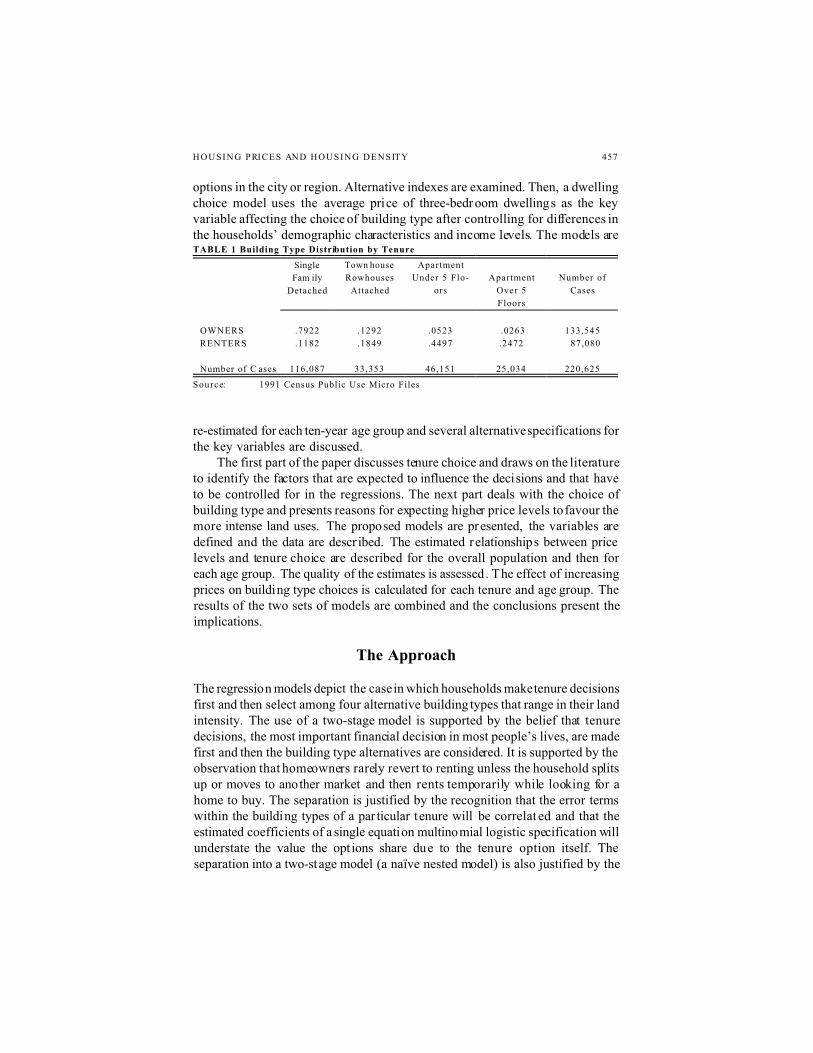
In Canada, homeownership rates declined between 1981 and 1996 forhouseholds whose primary maintainer was under 55 years of age. The largestdecline was in the 25 to 34 year-old group (51.62 to 46.06 percent) and then inthe 35 to 44 year-olds (71.67 to 66. 14 percent).3 Explanations for the changehave not yet been offered in the li terature but casual observat ion points to in-creasing housing prices in the largest cities and a reduction in the stability ofincome for many younger people. The demographic changes by themselves arenot expected to make cities more compact as the smaller family and the non-family households are still buying houses.4 In fact, non-family households haveincreased their rate of home purchase; young households with children arestaying longer in the rental sector. Systematic changes have not yet been ob-served in the mix of dwelling types offered on the market over the last ten years,but they are highly different iated across tenure categor ies as illustrated in Table1. Changes in tenure proportions can be expected to affect the mix of dwellingtypes and eventually the profiles of cit ies.
This study uses the 1991 Canadian Census Public Use Micro Data File tolook at the relationship between housing prices, tenure and the mix of dwellingtypes. Multinomial logistic models are estimated to describe the relationshipbetween price levels and the mix of building types within each tenure category.First, a tenure choice model is specified that focuses on the difference betweenthe price a household can reasonably afford and the average price of ownership
HOUSING PRICES AND HOUSING DENSITY 457
options in the city or region. Alternative indexes are examined. Then, a dwellingchoice model uses the average price of three-bedroom dwellings as the keyvariable affecting the choice of building type after controlling for differences inthe households’ demographic characteristics and income levels. The models areTABLE 1 Building Type Distribution by Tenure
Single
Fam ily
Detached
Town house
Rowhouses
Attached
Apartment
Under 5 Flo-
ors
Apartment
Over 5
Floors
Number of
Cases
OWNERS
RENTERS
.7922
.1182
.1292
.1849
.0523
.4497
.0263
.2472
133,545
87,080
Number of C ases 116,087 33,353 46,151 25,034 220,625
Source: 1991 Census Public Use Micro Files
re-estimated for each ten-year age group and several alternative specifications forthe key variables are discussed.
The first part of the paper discusses tenure choice and draws on the literatureto identify the factors that are expected to influence the decisions and that haveto be controlled for in the regressions. The next part deals with the choice ofbuilding type and presents reasons for expecting higher price levels to favour themore intense land uses. The proposed models are presented, the variables aredefined and the data are descr ibed. The estimated relationships between pricelevels and tenure choice are described for the overall population and then foreach age group. The quality of the estimates is assessed. The effect of increasingprices on building type choices is calculated for each tenure and age group. Theresults of the two sets of models are combined and the conclusions present theimplications.
The Approach
The regression models depict the case in which households make tenure decisionsfirst and then select among four alternative building types that range in their landintensity. The use of a two-stage model is supported by the belief that tenuredecisions, the most important financial decision in most people’s lives, are madefirst and then the building type alternatives are considered. It is supported by theobservation that homeowners rarely revert to renting unless the household splitsup or moves to another market and then rents temporarily while looking for ahome to buy. The separation is justified by the recognition that the error termswithin the building types of a par ticular tenure will be correlat ed and that theestimated coefficients of a single equation multinomial logistic specification willunderstate the value the opt ions share due to the tenure option itself. Theseparation into a two-stage model (a naïve nested model) is also justified by the
458 SKABU RSKIS
5. Comparing the 1996 with 1991 regressions might focus on temporal change. Pooled
regressions can be attempted. Stock optio ns m ight b e ente red a s a leg ged v ariab le constructed
by using earlier census statistics. Casual experiments that included time series of price indexes
and starts did yield immediate results but are worth experimenting with.
differences in the way the economic factors are specified in the tenure and thebuilding type decisions. In the tenure case, the emphasis might be on theconstraints created by the downpayment and the difficulty in getting a mortgage.In the choice of building type, the emphasis is on the price of a standard unit ofhousing services and all the factors that correlate with it.
The statistical models are estimated with cross-sectional data and theircoefficients are then used to develop inferences as to how price changes mightaffect behaviour. The difficul ties to overcome and the qualifications neededwhen basing predictions on cross-sectional data have been described bySkaburskis (1994). Among them are the assumptions that current markets are inequilibrium and that the mix of options across which people make choices havebeen developed under past conditions that reflect, in spatially relative terms, thecurrent conditions on which data is available. Space and time are assumed to besubstitutable. Adjustment times are ignored. Clearly these are heroic andunrealistic assumptions! The problematic aspect of the assumptions is, to anextent, diffused in three ways. First , we test many models to check forconsistency and robustness of results. Second, we break the samples into agegroups and look for the reasonableness of the differences in the impact of pricedifferences across the groups. Third, we enter in the logistic equations var iablesdescribing the logarithm of the number of dwellings in each city by eachbuilding type and tenure to control for the effects of stock legacy. Thecoefficients for the other variables in the regression are expected to show howpeople differ from each other across the specified attributes after controlling forthe effects of the range of choices that are available in their city. These steps domake the paper a tedious reading venture and this approach will not entirelyovercome the problem, but to do so properly would require us to wait for severalgenerations of additional census data. Other means for dealing with the problemwill be attempted in future research.5
Tenure Choice
The opportunity to become a homeowner is perhaps the most importantdeterminant of city form in Canada because of the difference in the buildingtypes that are typically associated with the two tenure options that are illustratedin Figure 1. Tenure choice is influenced by the household’s social and financialsituation as well as by housing market conditions. Increases in the price ofalmost any goods or services will eventually reduce its consumption if all other
HOUSING PRICES AND HOUSING DENSITY 459
6. Ha urin et al (1996), using a method developed by Linneman and Wachter (1989), estimate the
e las t ic ity of tenure choice with respect to the user cost of homeownership to be -. 93 .
Henderson and Ioannides (1989b) find a statistically significant relationship be tween rent
levels and the pro bability of homeow nersh ip bu t: “ …highe r ow ners hip p rices dram atically
increase the probability of renting. A 10 percent increase in owner prices from the mean of
.24 increases the probability of renting by 7 percent” (Henderson and Ioan nides (198 9b: 2 25).
The seven percent ratio is lower than the 9.3 percent estimated by Haurin et al, but
the seven percent applies to the whole population and not just the young.
7. In the short run a p rice increase may stimulate the demand for housing as an investment which
in turn fuels the price inflation until the bubble b ursts. Incr eases in hou sing p rice c reate wea lth
for homeowners and can fuel their expectations of continued price increases. Inflation makes
some homeowners move to larger houses in the hope of larger untaxed capital gains in the
future.
FIGURE 1 Dis tr ibut ion of Bui ld ing Types by Tenure in Canada CMAs and CAs
conditions and prices remain the same. 6 Increases in housing prices are associatedwith themarket’s move toward a new equilibrium in which households wouldconsume less housing relative to other goods and services. 7 A reduction inhousing consumption may mean that it selects a smaller house on a smaller lotor chooses a higher density dwelling type. Cities with higher overall housingprices due to their size, taxes, land-use policy, growth controls or naturalconstraints may be expected to have more dense profiles. However, the observedrelationship between the mix of building types and the differences in price levelsacross cities and regions cannot dir ectly be used to suggest that similar
460 SKABU RSKIS
differences will manifest over time in any one city should its housing priceschange. Many other factors may account for the price differences and may alsobe associated with differences in the distribution of tenure and building types.The statistical modelling attempts to control for the effects of the other factorsby including variables describing household characterist ics.
Even if the models were complete, the cities may be in different states intheir progress toward a market equilibr ium. Higher housing pr ices may not yethave manifested in a raised density profile and this factor cannot be accountedfor in a cross-sectional study. The effect of this factor has to be weighed againstthe possible effects of other conditions that may move the markets in theopposite direction. F urther work that tries to address the questions raised hereshould look at changes in dwelling type mix over time and relate these to pricemovements.
Perhaps the most important factor affecting a household’s tenure is itsincome level. Most households prefer larger rather than smaller dwellings andmost will select less dense dwelling types when they can afford the option. Asa result, higher income households are more likely to obtain the prefer red lowerdensity housing opt ions which will also have a higher price. Income differencesare, therefore, correlated with housing pr ice differences which are alsoassociated with differences in tenure and building type profi les. Income,permanent and transitory, is one of the key factors that has to be accounted forand the literature shows this to be a complicated variable.
Megbolugbe and Linneman (1993) point to the spuriousness of manypublished correlations between income and tenure choice and refer to Cooper-stein’s (1989) study showing the interrelationship among income level,household stability and home purchase. Henderson and Ioannides (1989) showthat older people, in larger families, who are white or married, have a betterchance of being homeowners. Kendig (1984) suggests that life cycle changes arecorrelated with improvements in the household’s economic means and finds that“the importance of the life cycle stage as a predictor of mobility and tenure ismarkedly reduced when factors related to financial resources are taken intoaccount” (p.272). The role of liquidity needs and downpayment constraints isillustrated by Artle and Varaiya (1978) and formally examined by Brueckner(1986). These constraints affect low-income households the most. Jones (1989)suggests that all differences between tenure options ar ise out of marketimperfections and Linneman and Megbolugbe (1992) show that wealthconstraints and market imperfections, are more important than income indetermining the tenure of low-income groups. Bourassa (1995), using Linnemanand Wachter’s (1989) approach, concludes that:
“…for constrained Australian households in the 25 to 34 age group, themagnitude of the borrowing constraint gap is inversely related to theprobability of ownership. Household expected income, transitoryincome and the relative cost of owning and renting have a smaller direct
HOUSING PRICES AND HOUSING DENSITY 461
8. Canadian ren te r s were shown to have $294 less in accumulated assets for every $1000
increase in housing costs (Engelhardt 1994)
impact…” (Bourassa 1995: 1172) [emphasis mine].
Data on all the factors affecting tenure choice are not available in theCanadian census but many of the factors are correlated with income and with thehousehold’s stage in its life cycle. The income variable will control fordifferences in the income levels across the regions and it will also account, to adegree, for differences in wealth, for the difficulty of making the downpayment,for ability to access financing, and for the household’s stability. Tastedifferences may also be associated with income but so far there is no evidencepointing to which income groups have the higher preference for homeownership.Since most of the effects that correlate with income are expected to decrease intheir importance as incomes rise, income squared is also a relevant variable inthe tenure choice model. Including variables describing income, life-cycle stageand family type in the logistic regression will reduce the extent that the non-pr icefactors cloud the relationships of interest, but completely unbiased estimates arebeyond reach at this time.
Increasing housing prices relative to income forces young households to savefor longer periods of time to accumulate their downpayment. The people who dosave for a downpayment tend to reduce their rate of savings in response toincreasing housing prices. 8 Higher prices will delay home purchase and, thereby,reduce the proportion of owner occupied buildings in the city compared to whatit would otherwise be. The effect of the downpayment constraints i s, to anextent, determined by the level of housing prices and increasing prices mayincrease the importance of the constraint causing the estimated coefficients to bebiased unless the endogeneity is accounted for.
Income levels and household formation are also endogenous and areaffected, to an extent, by housing prices. Haurin et al (1996) show that husbandsand wives work longer hours at the time they buy their house. Fort in (1995)shows that the household’s commitment to a mortgage induces more wives towork outside the home while the mortgage is being paid off. Haurin et al (1996)and Kim (1992) identify the influence of housing prices on young people’stendency to form independent households, and Skaburskis (1994) illustrates theconnection using Canadian data. In addition, after leaving home, incomeprospects affect family formation and fertility (Skaburskis 1996). The extent ofthe endogeneity is expected to be small and we might be able to gauge itspossible magnitude by seeing how the sequential introduction of controlvariables change the estimated coefficients for the price variable. But there ismore.
Mayer and Engelhardt (1996) show that the role of gifts has become moreimportant to first-time buyers and half in a sample received substantial help from
462 SKABU RSKIS
relatives and friends (Engelhardt and Mayer 1994, 1998). Income, the propensityto save, the receipt of gifts, and the size of down payments are affected byhousing prices in ways that have changed over time. Not only does the recentliterature show the extent of the spurious correlations due to our lack ofknowledge of the complexity of housing markets and household decisions, butit also shows that we can have no assurance that past correlations will continueinto the future. To the extent that new factors emerge to mediate the impact ofthe trends that would prevent young people from attaining homeownership, it islikely that the changes correctly attributed to price differences in a study of pastconditions will overstate the effects of future price changes.
The Choice of Building Type
Increasing prices and rents are expected to make households within each tenuregroup reduce their housing consumption. People who are buying thei r first homeare likely to buy a smaller house, on less land, after prices increase. Singell andLillydahl (1990), for example, find that the average lot size for houses in theirColorado case study decreased by 10 percent after development impact fees wereintroduced.
The theoretical basis for the connection between prices and dwelling mix isfound in the early neoclassical location theory. As price levels rise, people cutback on their housing purchases, thereby, changing their spat ial equilibrium.After buying smaller quantities of housing services, households may find that itis worth their while to move closer to the city centre, pay a little more for eachunit of housing service but reduce commute costs by a fixed amount, by anamount that was in equilibrium with the old price structure in the case of themonocentric city (Alonso 1964). Increases in the housing price levels areexpected to increase the curl of the price/distance gradient and raise land valuesmost near the city centre (Muth 1969). Higher urban growth r ates or theexpectation of high future growth rates will also raise land prices and encouragemore dense forms of development (Arnott 1980). Higher land values induced byan overall price increase lead to higher densities directly and indirectly throughthe induced shift toward the centre in the case of monocentric cit ies. Muchsmaller effects would be expected in the case of multi-nuclear cities. The effectsof a price increase on a household’s spatial equilibrium is expected to differacross income groups with lower income household’s choices being affected themost.
The published empirical evidence confirms the connection between housingprices and density. John Quigley examines the choice of building type andestimates the coefficients for a multinomial logit (MNL) model using Pittsburghdata. He shows that “larger families with greater demands for necessities aremore responsive to relative price in the choice of housing type” (Quigley 1973:
HOUSING PRICES AND HOUSING DENSITY 463
9. For lower income households, the probability of selecting an apartment declines from .84 for
a one- pers on h ouse hold to . 06 fo r a fiv e-per son h ouse hold ; the pro bability of sele cting a unit
with a com mon w all increases fr om . 11 to . 69; an d the pro bability of c hoosing a detached
house increases from .04 to .25 (Quigley 1973). His data do not yield low variance
coeff icients for the higher income groups but they do show that hig her income households
“system atically choose less dense ho using configura tions”.
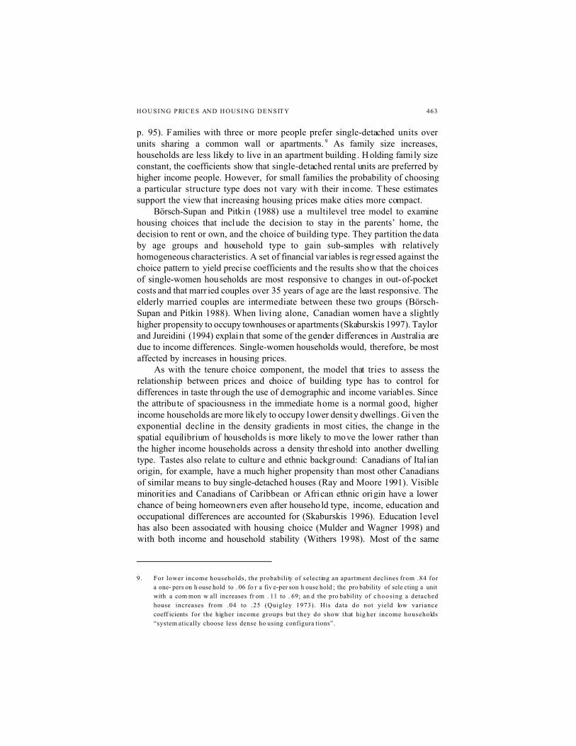
p. 95). Families with three or more people prefer single-detached units overunits sharing a common wall or apartments. 9 As family size increases,households are less likely to live in an apartment building. Holding family sizeconstant, the coefficients show that single-detached rental units are preferred byhigher income people. However, for small families the probability of choosinga particular structure type does not vary with their income. These estimatessupport the view that increasing housing prices make cities more compact.
Börsch-Supan and Pitkin (1988) use a multilevel tree model to examinehousing choices that include the decision to stay in the parents’ home, thedecision to rent or own, and the choice of building type. They partition the databy age groups and household type to gain sub-samples with relativelyhomogeneous characteristics. A set of financial var iables is regr essed against thechoice pattern to yield precise coefficients and the results show that the choicesof single-women households are most responsive to changes in out-of-pocketcosts and that marr ied couples over 35 years of age are the least responsive. Theelderly married couples are intermediate between these two groups (Börsch-Supan and Pitkin 1988). When living alone, Canadian women have a slightlyhigher propensity to occupy townhouses or apartments (Skaburskis 1997). Taylorand Jureidini (1994) explain that some of the gender differences in Australia aredue to income differences. Single-women households would, therefore, be mostaffected by increases in housing prices.
As with the tenure choice component, the model that tries to assess therelationship between prices and choice of building type has to control fordifferences in taste through the use of demographic and income variables. Sincethe attribute of spaciousness in the immediate home is a normal good, higherincome households are more likely to occupy lower density dwellings. Given theexponential decline in the density gradients in most cities, the change in thespatial equilibrium of households is more likely to move the lower rather thanthe higher income households across a density threshold into another dwellingtype. Tastes also relate to culture and ethnic background: Canadians of Ital ianorigin, for example, have a much higher propensity than most other Canadiansof similar means to buy single-detached houses (Ray and Moore 1991). Visibleminorit ies and Canadians of Caribbean or African ethnic origin have a lowerchance of being homeowners even after household type, income, education andoccupational differences are accounted for (Skaburskis 1996). Education levelhas also been associated with housing choice (Mulder and Wagner 1998) andwith both income and household stability (Withers 1998). Most of the same
464 SKABU RSKIS
10. The 10 percent interest rate is typical of the rates that were changed during the preceding five
years. In Canada, mortgage terms longer than five years were not available. The conclusions
are not sensitive to reasonable changes in the rate.
11. The variable G A P . U N D E R tells by how much the market price is above the price the
household can afford by our definition of affordability. It takes the value of zero when the
hou seho ld can afford the market price. The GAP-OVER tells by how much the hous ehold’s
income is in excess of the market price for the standardized house and take the value of zero
when the househo ld ’s income is below the market price. This variable will always have a
negative value as the GAP variables are constructed by subtracting from the market price the
affordable price.
12. The relationship between the size of the GAP and the household’s tenure status is expected
to be S-s hape d. The varia bles w ere e ntere d in q uadr atic fo rm. While these specifications
yielded estimates for all coefficients except the GAP.U NDER. SQUARED variable that were
differ ent fr om z ero a t the . 001 pro bability level and improved the fit of the model using all
cases, they did not yield good results when the models were estimated for each age group. The
coefficient for the GAP.OVE R.SQUARE D variable was positive indica ting th at incr eases in
the GAP, when the affordable price is above the mean value of dwellings in the region,
quickly led toward homeownership.
13. An alternative specification considered the difference between the a f fo rdable price and the
value of the dwellings occupied by younger households with the same size of ho useh old. This
allowed the bedrooms to vary in the index as a function of the households’ needs for space.
The magnitude of the difficulty in attaining hom eow ners hip is, in par t, a function of the size
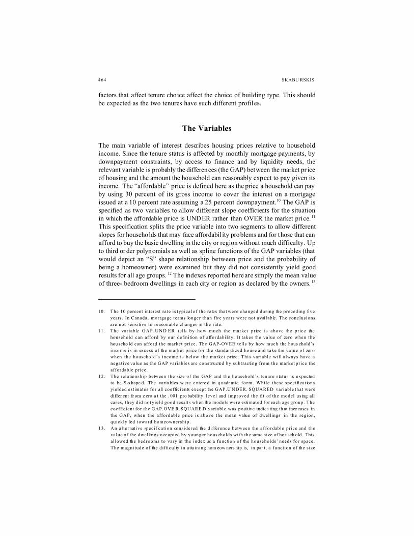
factors that affect tenure choice affect the choice of building type. This shouldbe expected as the two tenures have such different profiles.
The Variables
The main variable of interest describes housing prices relative to householdincome. Since the tenure status is affected by monthly mortgage payments, bydownpayment constraints, by access to finance and by liquidity needs, therelevant variable is probably the differences (the GAP) between the market pr iceof housing and the amount the household can reasonably expect to pay given itsincome. The “affordable” price is defined here as the price a household can payby using 30 percent of its gross income to cover the interest on a mortgageissued at a 10 percent rate assuming a 25 percent downpayment.10 The GAP isspecified as two variables to allow different slope coefficients for the situationin which the affordable pr ice is UNDER rather than OVER the market price.11
This specification splits the price variable into two segments to allow differentslopes for households that may face affordabil ity problems and for those that canafford to buy the basic dwelling in the city or region without much difficulty. Upto third or der polynomials as well as spline functions of the GAP var iables (thatwould depict an “S” shape relationship between price and the probability ofbeing a homeowner) were examined but they did not consistently yield goodresults for all age groups. 12 The indexes reported here are simply the mean valueof three- bedroom dwellings in each city or region as declared by the owners. 13
HOUSING PRICES AND HOUSING DENSITY 465
of the dwe l l ing the household hopes to buy. Since the categorical variables describing
hou seho ld sizes and age g rou ps ar e ente red in the re gres sions that de velop ed this index along
with the categorical variables identifying cities, the household size and age variables change
the level of the index faced by similar households but not the relative prices across cities and
regions. This specification did not yield quite as good results as the mean price of three-
bedr oom units a cros s all the sub-p opu lations that w ere lo oked at.
The mean price variable used here is a trimmed mean as household incomes are
truncated in the PUM F at the upper end to maintain confidentiality. Half (49.57 percent) of
all own ersh ip units have three bedrooms and the distribution across the four types is 50.41%,
5 8. 5 0% , 32.30% and 16. 07% for high rise condominiums. More than half (55.80%) of high-
rise cond omin iums have only two b edro oms . E xper imen ts with the room coun ts did n ot yield
notab le differences. The average number of bedrooms varies across the metropolitan areas of
Canada from a low of 2.94 in Montreal to a high of 3.30 in Calgary and in Edmonton.
14. Bourassa (1994) finds that imm igran ts to Au stralia, after a ccou nting for d iffere nces in endow-
men t, have the same or higher propensities to be homeowners than the Australian-born popu-
lation.
Four alternative constructions for the price variable are examined and reportedto test for the robustness of the conclusions.
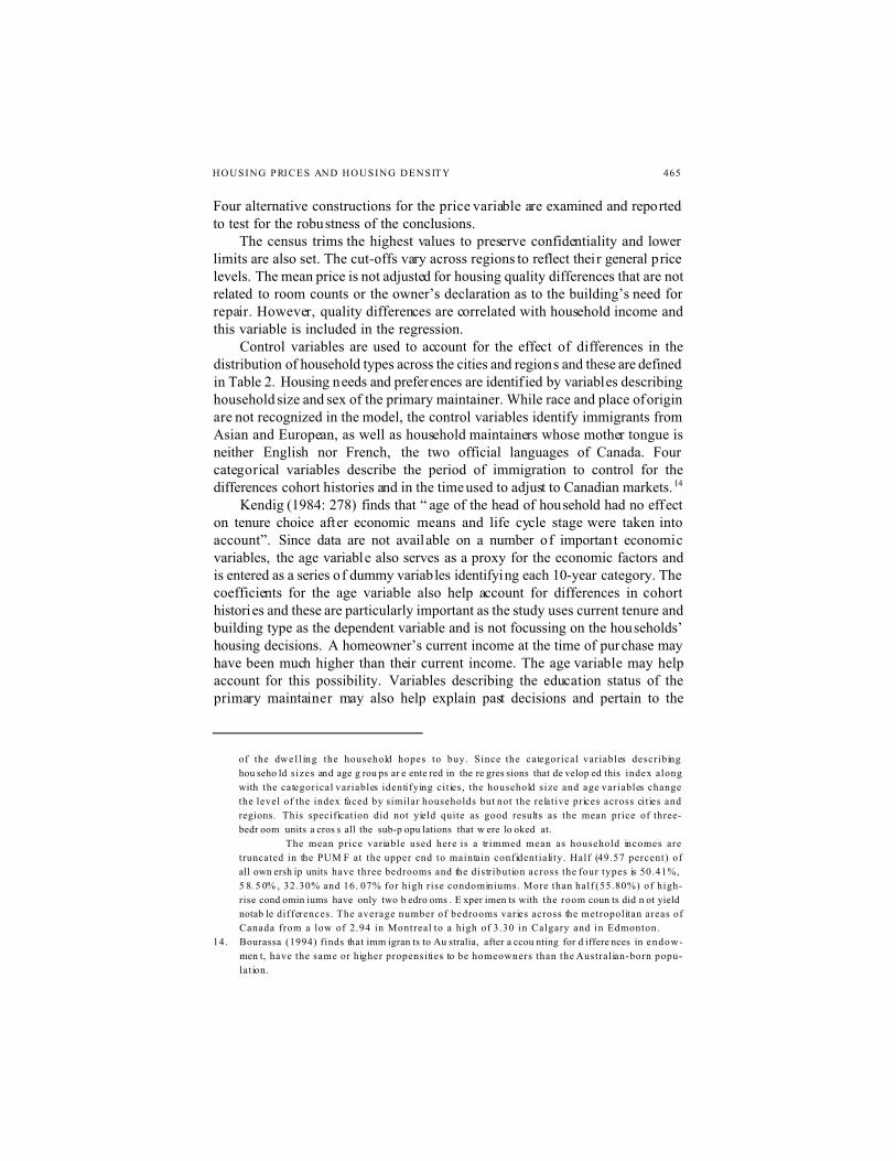
The census trims the highest values to preserve confidentiality and lowerlimits are also set. The cut-offs vary across regions to reflect their general pricelevels. The mean price is not adjusted for housing quality differences that are notrelated to room counts or the owner’s declaration as to the building’s need forrepair. However, quality differences are correlated with household income andthis variable is included in the regression.
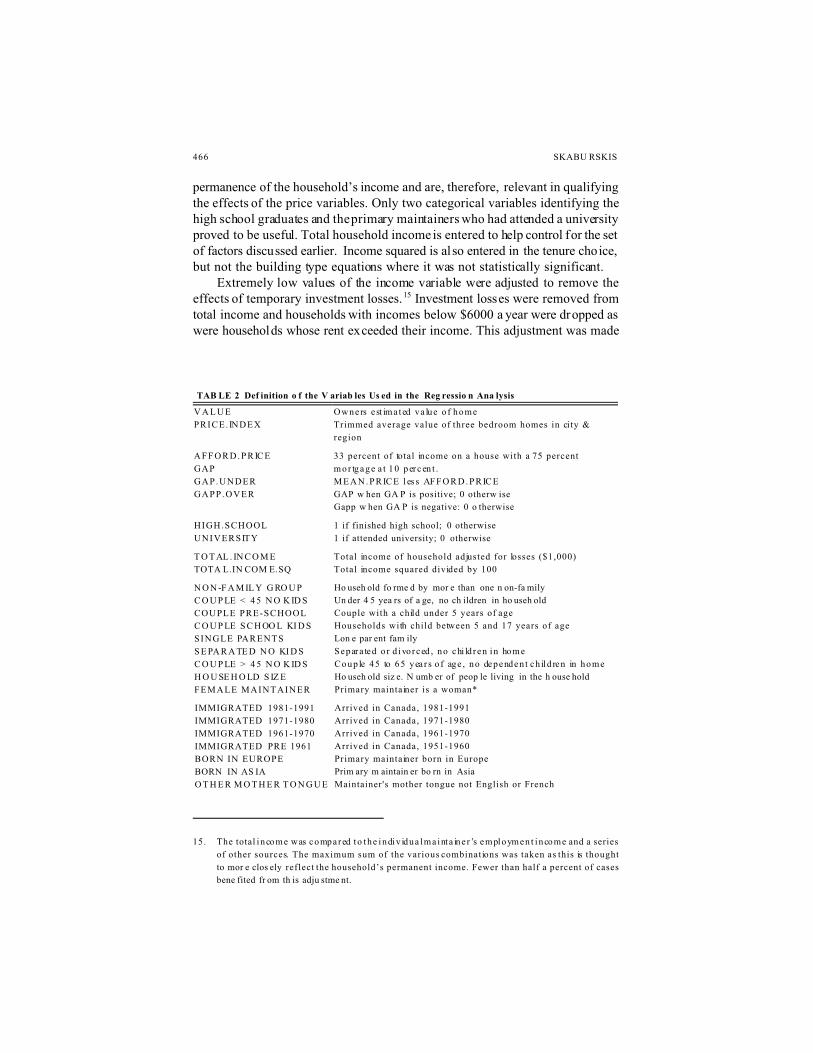
Control variables are used to account for the effect of differences in thedistribution of household types across the cities and regions and these are definedin Table 2. Housing needs and preferences are identif ied by variables describinghousehold size and sex of the primary maintainer. While race and place of originare not recognized in the model, the control variables identify immigrants fromAsian and European, as well as household maintainers whose mother tongue isneither English nor French, the two official languages of Canada. Fourcategorical variables describe the period of immigration to control for thedifferences cohort histories and in the time used to adjust to Canadian markets. 14
Kendig (1984: 278) finds that “ age of the head of household had no effecton tenure choice after economic means and life cycle stage were taken intoaccount”. Since data are not available on a number of important economicvariables, the age variable also serves as a proxy for the economic factors andis entered as a series of dummy variables identifying each 10-year category. Thecoefficients for the age variable also help account for differences in cohorthistories and these are particularly important as the study uses current tenure andbuilding type as the dependent variable and is not focussing on the households’housing decisions. A homeowner’s current income at the time of purchase mayhave been much higher than their current income. The age variable may helpaccount for this possibility. Variables describing the education status of theprimary maintainer may also help explain past decisions and pertain to the
466 SKABU RSKIS
15. The total i ncome was compared to t he indiv idua l ma int a ine r ’s employmen t i ncome and a series
of other sources. The maximum sum of the various combinations was taken as this is thought
to mor e clos ely reflect the household’s permanent income. Fewer than half a percent of cases
bene fited fr om th is adju stme nt.
permanence of the household’s income and are, therefore, relevant in qualifyingthe effects of the price variables. Only two categorical variables identifying thehigh school graduates and the primary maintainers who had attended a universityproved to be useful. Total household income is entered to help control for the setof factors discussed earlier. Income squared is also entered in the tenure choice,but not the building type equations where it was not statistically significant.
Extremely low values of the income variable were adjusted to remove theeffects of temporary investment losses.15 Investment losses were removed fromtotal income and households with incomes below $6000 a year were dropped aswere households whose rent exceeded their income. This adjustment was made
TAB LE 2 Def inition o f the V ariab les Us ed in the Reg ressio n Ana lysis
V A L U E
PRICE. INDEX
Owners e st ima ted va lue o f home
Trimmed average value of three bedroom homes in city &
region
A F F O R D . P R IC E
GAP
GAP.UNDER
GAPP.OVER
33 percent of total income on a house with a 75 percent
m o r tg a g e a t 1 0 p er c en t .
M E A N . P R IC E l es s AF F O R D . P R IC E
GAP w hen GA P is positive; 0 otherw ise
Gapp w hen GA P is negative: 0 o therwise
HIGH.SCHOOL
UNIVERSITY
1 if finished high school; 0 otherwise
1 if attended university; 0 otherwise
T O T AL . IN C O M E
TOTA L.IN COM E.SQ
Total income of household adjusted for losses ($1,000)
Total income squared divided by 100
N O N -F A M IL Y G RO U P
C O U P LE < 4 5 N O K ID S
COUPLE PRE-SCHOOL
C O U P LE S C H OO L KI D S
SINGLE PARENTS
S E PA R A TE D N O KI D S
C O U P LE > 4 5 N O K ID S
H O U SE H O LD S IZ E
FEMALE MAINTAINER
Ho useh old fo rme d by mor e than one n on-fa mily
Un der 4 5 yea rs of a ge, no ch ildren in ho useh old
Couple with a child under 5 years of age
Households with child between 5 and 17 years of age
Lon e par ent fam ily
Separa ted o r d ivo rced , no chi ld ren in home
Coup le 45 to 65 yea r s o f age , no dependen t ch ild ren in home
Ho useh old siz e. N umb er of peop le living in the h ouse hold
Primary maintainer is a woman*
IMMIGRATED 1981-1991
IMMIGRATED 1971-1980
IMMIGRATED 1961-1970
IMMIGRATED PRE 1961
BORN IN EUROPE
BORN IN AS IA
O T H E R M O T H E R T O N G U E
Arrived in Canada, 1981-1991
Arrived in Canada, 1971-1980
Arrived in Canada, 1961-1970
Arrived in Canada, 1951-1960
Primary maintainer born in Europe
Prim ary m aintain er bo rn in Asia
Maintainer's mother tongue not English or French
HOUSING PRICES AND HOUSING DENSITY 467
16. Households were excluded if they earned less than $6,000 during 1990 as such levels are too
small to allow effective participation in the housing market and are, therefore, thought of as
instances of either inaccurate reporting of income or of the r eporting of tempo rary loss es. It
is also thought that most households reporting incomes below $500 a month represent special
cases such as students and people living on the remittances that they did not include a s income
in their census questionnaire. The census does not have a “homeless category”. Households
reporting income that was lower than their rent were also excluded. The exclusion of the lower
income households d oes not particularly bias the average as the upper end of incomes are
truncated in the available census data.
In a national su rvey of condominium occupants, I traced the respondents who
reported incomes that were lower than their rents and found, in most cases, that other people,
mos tly their children, were paying their rent for them and they did not see this payment as
‘income ’. In another survey, net revenue from secondary suites in houses or sm all mu ltiple
converted dwellings appeared to us as not being thought of as “income” by man y respond ents.
Fewer than 2 perc ent of hou seho lds in the Canadian census report negative incomes and these
were excluded unless the individual or the sum of the maintainer’s wages, transfers or “other”
income was positive.
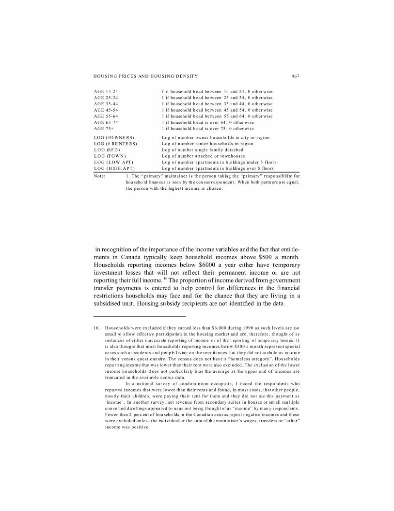
AGE 15-24
AGE 25-34
AGE 35-44
AGE 45-54
AGE 55-64
AGE 65-74
AGE 75+
1 if household h ead between 15 and 24 , 0 other wise
1 if household h ead between 25 and 34 , 0 other wise
1 if household h ead between 35 and 44 , 0 other wise
1 if household h ead between 45 and 54 , 0 other wise
1 if household h ead between 55 and 64 , 0 other wise
1 if household h ead is over 64 , 0 other wise
1 if household h ead is over 75 , 0 other wise
LOG (#O WNE RS)
LOG (# RE NTE RS)
L O G (S F D )
L O G (T O W N )
LOG (LOW.APT)
LOG (HIGH.APT)
Log of number owner households in city or region
Log of number renter households in region
Log of number single family detached
Log of number attached or townhouses
Log of number apartments in buildings under 5 floors
Log of number apartments in buildings over 5 floors
Note: 1. The “ primary” maintainer is the person taking the “primary” responsibility for
hou seho ld finan ces as seen by th e cen sus r espo nden t. When both partn ers a re eq ual,
the person with the highest income is chosen.
in recognition of the importance of the income variables and the fact that enti tle-ments in Canada typically keep household incomes above $500 a month.Households reporting incomes below $6000 a year either have temporaryinvestment losses that wil l not reflect their permanent income or are notreporting their ful l income. 16 The proportion of income derived from governmenttransfer payments is entered to help control for dif ferences in the financialrestrictions households may face and for the chance that they are living in asubsidised unit. Housing subsidy recipients are not identified in the data.
468 SKABU RSKIS
17. I am grateful to the journal’s referees for the suggestion to test fo r the robus tness o f the GAP
and the price/income ratio variables. The price and rent indexes take on only 40 different
values. The main variation in the ratio in dexe s and the G AP v ariab les ar e due to t he income
variation. The GAP spec ification in the tenure case survives the tests and yields similar resu lts
that are very similar to ones obtained by using price alone.
18. Attem pts to adju st for q uality b y con sider ing th e num ber o f bed roo ms, num ber o f roo ms, state
of repair, length of oc cupa ncy to acco unt fo r tenu re dis coun t did n ot imp rov e the e stimate
coefficients for the rent index.
19. The coeff icients for the rent in dex, after a ccou nting for in com e in the regr ession , co nsisten tly
associated higher prices with a decrea se in the pr oportion of low-rise a partme nts. In Canada,
this is the lowest cost building type that includes four-storey (three-storey, wood frame above
grade and one concr ete below) walk-up s without elevators.
The same control variables except for income squared and the proportion ofincome derived from government transfers are used when looking at the effectof price differences on the distribution of building types within each tenurecategory. The key variable that is derived from profit maximizing conditions byCho (1997) is housing price divided by household income. Experiments with theprice and the rent- to-income ratio developed low variance and apparently good-looking coefficients for the dwelling type distributions for each tenure and foreach age group until income was also entered as a separate control variable tohelp account for the dwelling quality differences that are correlated with income.The income variable swamped the estimates for the price/income ratio in bothtenure categories. 17 The index using the city’s or region’s mean rent did notdevelop interesting coefficients for the dwelling type options within the rentertenure. 18 In most cases, they were indistinguishable from zero despite the hugesample. 19 As a result, the price index is used to assess the effect of pricedifferences on the mix of residential building types in both the owner and rentercategories. Its use is justified by the fact that rents in more than a half ofCanada’s rental stock were under control in 1991 and market differences maymanifest primari ly as differences in access to suitable units. Housing pricedifferences may, therefore, be a good indication of differences in the tightnessof rental markets and it is this that may affect the household’s choice of dwellingtype.
A serious concern is created by the possible confounding of the value of thebuilding type options with the valuation of the tenure options. A household’sdecision to buy a house may be affected by the fact that there are many moredwellings available in the ownership market than in the rental market. Similarly,the number of units within each building type affect the degree of choice offeredwithin each dwelling type. One way of accounting for the effect of thesedifferences is to include variables describing the natural logarithm of the numberof dwellings available within each option. John Quigley’s(1976) inclusion ofthese variables is commented on by Daniel McFadden(1978). More sophisticatedmodels that incorporate estimates that reflect the value of the housing optionswithin each tenure category as well as the variation in that value could not be
HOUSING PRICES AND HOUSING DENSITY 469
20. Attem pts to con struc t the thr ee co mpo nents of the inclus ive ter m tha t rese mble the ones in
McF adden ’s (1978) usi ng SAS failed as they led to a complete separation of the tenure
categories. The coefficient for the log of the number of buildings is equal to 1-* , where * is
a measure of the extent that buildings in the class are seen as being similar. Ideally the log of
the number of buildings in the option is entered wi th a coefficient restricted to one. The
estima ted co efficien ts are close to on e in the case o f the ten ure c hoice mod el.
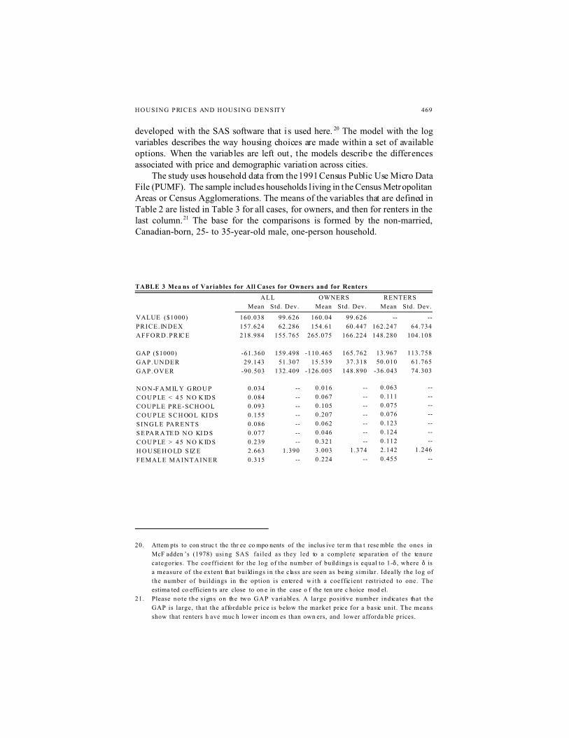
21. Please no te the s igns on the two GAP variables. A la rge positive number indicates that the
GAP is large, that the affordable price is below the market price for a basic unit . The means
show that renters h ave muc h lower incom es than own ers, and lower afforda ble prices.
developed with the SAS software that i s used here. 20 The model with the logvariables describes the way housing choices are made within a set of availableoptions. When the variables are left out , the models describe the differencesassociated with price and demographic variation across cities.
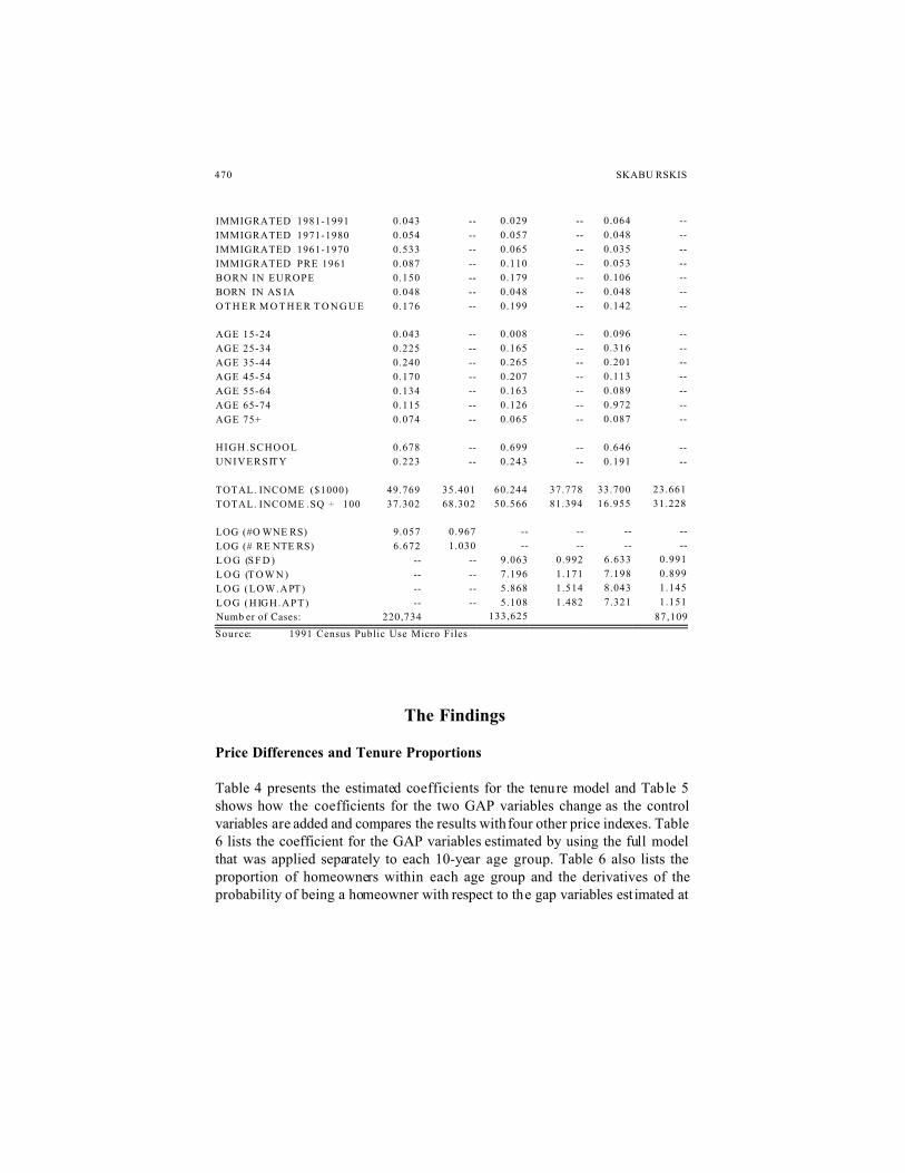
The study uses household data from the 1991 Census Public Use Micro DataFile (PUMF). The sample includes households l iving in the Census MetropolitanAreas or Census Agglomerations. The means of the variables that are defined inTable 2 are listed in Table 3 for all cases, for owners, and then for renters in thelast column.21 The base for the comparisons is formed by the non-married,Canadian-born, 25- to 35-year-old male, one-person household.
TABLE 3 Mea ns of Variables for All Cases for Owners and for Renters
ALL OWNERS RENTERS
Mean Std. Dev. Mean Std. Dev. Mean Std. Dev.
VALUE ($1000)
PRICE. INDEX
A F F O R D . P R IC E
160.038
157.624
218.984
99.626
62.286
155.765
160.04
154.61
265.075
99.626
60.447
166.224
--
162.247
148.280
--
64.734
104.108
GAP ($1000)
GAP.UNDER
GAP.OVER
-61.360
29.143
-90.503
159.498
51.307
132.409
-110.465
15.539
-126.005
165.762
37.318
148.890
13.967
50.010
-36.043
113.758
61.765
74.303
N O N -F A M IL Y G RO U P
C O U P LE < 4 5 N O K ID S
COUPLE PRE-SCHOOL
C O U P LE S C H OO L KI D S
SINGLE PARENTS
S E PA R A TE D N O KI D S
C O U P LE > 4 5 N O K ID S
H O U SE H O LD S IZ E
FEMALE MAINTAINER
0.034
0.084
0.093
0.155
0.086
0.077
0.239
2.663
0.315
--
--
--
--
--
--
--
1.390
--
0.016
0.067
0.105
0.207
0.062
0.046
0.321
3.003
0.224
--
--
--
--
--
--
--
1.374
--
0.063
0.111
0.075
0.076
0.123
0.124
0.112
2.142
0.455
--
--
--
--
--
--
--
1.246
--
470 SKABU RSKIS
IMMIGRATED 1981-1991
IMMIGRATED 1971-1980
IMMIGRATED 1961-1970
IMMIGRATED PRE 1961
BORN IN EUROPE
BORN IN AS IA
O T H E R M O T H E R T O N G U E
0.043
0.054
0.533
0.087
0.150
0.048
0.176
--
--
--
--
--
--
--
0.029
0.057
0.065
0.110
0.179
0.048
0.199
--
--
--
--
--
--
--
0.064
0.048
0.035
0.053
0.106
0.048
0.142
--
--
--
--
--
--
--
AGE 15-24
AGE 25-34
AGE 35-44
AGE 45-54
AGE 55-64
AGE 65-74
AGE 75+
0.043
0.225
0.240
0.170
0.134
0.115
0.074
--
--
--
--
--
--
--
0.008
0.165
0.265
0.207
0.163
0.126
0.065
--
--
--
--
--
--
--
0.096
0.316
0.201
0.113
0.089
0.972
0.087
--
--
--
--
--
--
--
HIGH.SCHOOL
UNIVERSITY
0.678
0.223
--
--
0.699
0.243
--
--
0.646
0.191
--
--
TOTAL. INCOME ($1000)
TOTAL. INCOME .SQ ÷ 100
49.769
37.302
35.401
68.302
60.244
50.566
37.778
81.394
33.700
16.955
23.661
31.228
LOG (#O WNE RS)
LOG (# RE NTE RS)
L O G (S F D )
L O G (T O W N )
LOG (LOW.APT)
LOG (HIGH.APT)
9.057
6.672
--
--
--
--
0.967
1.030
--
--
--
--
--
--
9.063
7.196
5.868
5.108
--
--
0.992
1.171
1.514
1.482
--
--
6.633
7.198
8.043
7.321
--
--
0.991
0.899
1.145
1.151
Numb er of Cases: 220,734133,625
87,109
Source: 1991 Census Public Use Micro Files
The Findings
Price Differences and Tenure Proportions
Table 4 presents the estimated coefficients for the tenure model and Table 5shows how the coefficients for the two GAP variables change as the controlvariables are added and compares the results with four other price indexes. Table6 lists the coefficient for the GAP variables estimated by using the full modelthat was applied separately to each 10-year age group. Table 6 also lists theproportion of homeowners within each age group and the derivatives of theprobability of being a homeowner with respect to the gap variables est imated at
HOUSING PRICES AND HOUSING DENSITY 471
22. The derivative in this case is equal to the estimated coefficient multiplied by the pro bability
the household was an owner and also multiplied by the probability the household was a renter.
the mean proportion for each age group.22
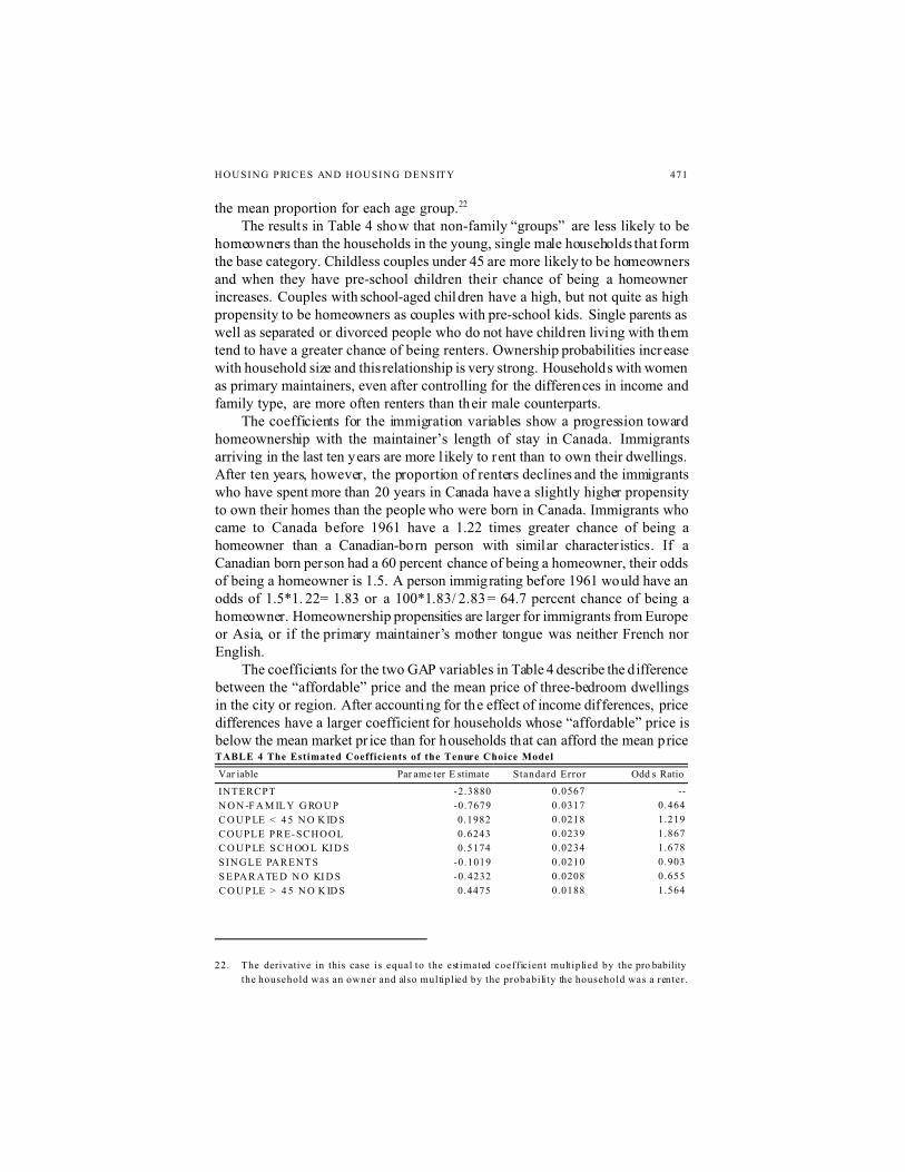
The results in Table 4 show that non-family “groups” are less likely to behomeowners than the households in the young, single male households that formthe base category. Childless couples under 45 are more likely to be homeownersand when they have pre-school children their chance of being a homeownerincreases. Couples with school-aged children have a high, but not quite as highpropensity to be homeowners as couples with pre-school kids. Single parents aswell as separated or divorced people who do not have children living with themtend to have a greater chance of being renters. Ownership probabilities increasewith household size and this relationship is very strong. Households with womenas primary maintainers, even after controlling for the differences in income andfamily type, are more often renters than their male counterparts.
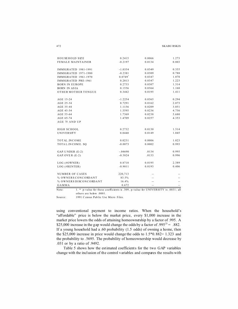
The coefficients for the immigration variables show a progression towardhomeownership with the maintainer’s length of stay in Canada. Immigrantsarriving in the last ten years are more l ikely to rent than to own their dwellings.After ten years, however, the proportion of renters declines and the immigrantswho have spent more than 20 years in Canada have a slightly higher propensityto own their homes than the people who were born in Canada. Immigrants whocame to Canada before 1961 have a 1.22 times greater chance of being ahomeowner than a Canadian-born person with similar character istics. If aCanadian born person had a 60 percent chance of being a homeowner, their oddsof being a homeowner is 1.5. A person immigrating before 1961 would have anodds of 1.5*1. 22= 1.83 or a 100*1.83/ 2.83= 64.7 percent chance of being ahomeowner. Homeownership propensities are larger for immigrants from Europeor Asia, or if the primary maintainer’s mother tongue was neither French norEnglish.
The coefficients for the two GAP variables in Table 4 describe the differencebetween the “affordable” price and the mean price of three-bedroom dwellingsin the city or region. After accounting for the effect of income differences, pricedifferences have a larger coefficient for households whose “affordable” price isbelow the mean market pr ice than for households that can afford the mean priceTABLE 4 The Estimated Coefficients of the Tenure Choice Model
Var iable Par ame ter E stimate Standard Error Odd s Ratio
INTERCPT
N O N -F A M IL Y G RO U P
C O U P LE < 4 5 N O K ID S
COUPLE PRE-SCHOOL
C O U P LE S C H OO L KI D S
SINGLE PARENTS
S E PA R A TE D N O KI D S
C O U P LE > 4 5 N O K ID S
-2.3880
-0.7679
0.1982
0.6243
0.5174
-0.1019
-0.4232
0.4475
0.0567
0.0317
0.0218
0.0239
0.0234
0.0210
0.0208
0.0188
--
0.464
1.219
1.867
1.678
0.903
0.655
1.564
472 SKABU RSKIS
H O U SE H O LD S IZ E
FEMALE MAINTAINER
0.2415
-0.2197
0.0066
0.0134
1.273
0.803
IMMIGRATED 1981-1991
IMMIGRATED 1971-1980
IMMIGRATED 1961-1970
IMMIGRATED PRE-1961
BORN IN EUROPE
BORN IN AS IA
O T H E R M O T H E R T O N G U E
-1.0354
-0.2381
0.0749 *
0.2013
0.2733
0.1556
0.3442
0.0349
0.0309
0.0347
0.0347
0.0307
0.0364
0.0195
0.355
0.788
1.078
1.223
1.314
1.168
1.411
AGE 15-24
AGE 25-34
AGE 35-44
AGE 45-54
AGE 55-64
AGE 65-74
A G E 75 A N D U P
-1.2254
0.7291
1.1156
1.5595
1.7369
1.4709
0.0365
0.0162
0.0209
0.0236
0.0238
0.0257
0.294
2.073
3.051
4.756
5.680
4.353
HIGH SCHOOL
UNIVERSITY
0.2732
0.0440
0.0130
0.0149
1.314
1.045
T O T AL . IN C O M E
TOTA L.IN COM E. SQ
0.0231
-0.0073
0.0006
0.0002
1.023
0.993
GAP.U NDER (E-2)
GAP.OVE R (E-2)
-.04690
-0.3824
.0134
.0133
0.995
0.996
LOG (#OWNER)
LOG (#RENTER)
0.8710
-0.9011
0.0195
0.0193
2.389
0.406
NUMBER OF CASES
% O W N E R S C O N C O RD A N T
% O W N E R S D I SC O N C O RD A N T
G A M M A
220,713
83.5%
16.4%
0.672
--
--
--
--
--
--
--
--
Note: 1. * p-value for these coefficients is .309, p-value for UNIVERSITY is .0031; all
others are below .0001.
Source: 1991 C ensus Pub lic Use Micro Files.
using conventional payment to income ratios. When the household’s“affordable” price is below the market price, every $1,000 increase in themarket price lowers the odds of attaining homeownership by a factor of .995. A$25,000 increase in the gap would change the odds by a factor of .99525 = .882.If a young household had a .60 probability (1.5 odds) of owning a home, thenthe $25,000 increase in price would change the odds to 1.5*0. 882= 1.323 andthe probability to .5695. The probability of homeownership would decrease by.031 or by a ratio of .9492.
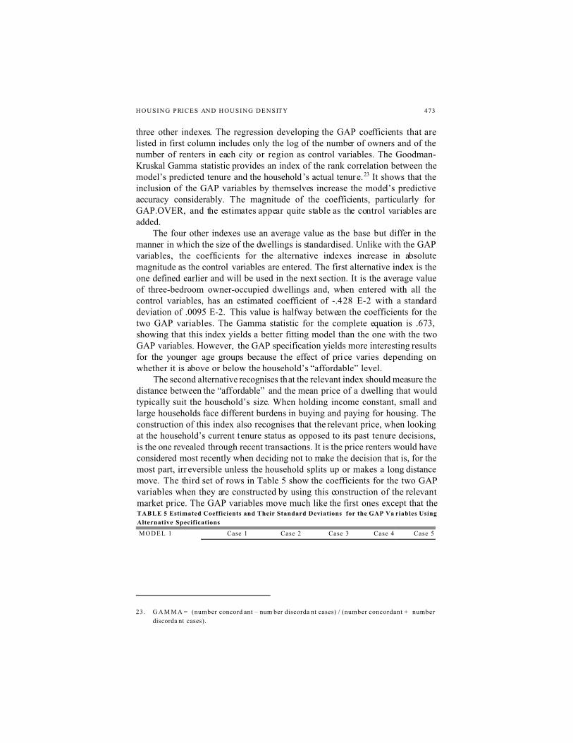
Table 5 shows how the est imated coefficients for the two GAP variableschange with the inclusion of the control variables and compares the results with
HOUSING PRICES AND HOUSING DENSITY 473
23. G A M M A = (number concord ant – num ber discorda nt cases) / (number concordant + number
discorda nt cases).
three other indexes. The regression developing the GAP coefficients that arelisted in first column includes only the log of the number of owners and of thenumber of renters in each city or region as control variables. The Goodman-Kruskal Gamma statistic provides an index of the rank correlation between themodel’s predicted tenure and the household’s actual tenure.23 It shows that theinclusion of the GAP variables by themselves increase the model’s predictiveaccuracy considerably. The magnitude of the coefficients, particularly forGAP.OVER, and the estimates appear quite stable as the control variables areadded.
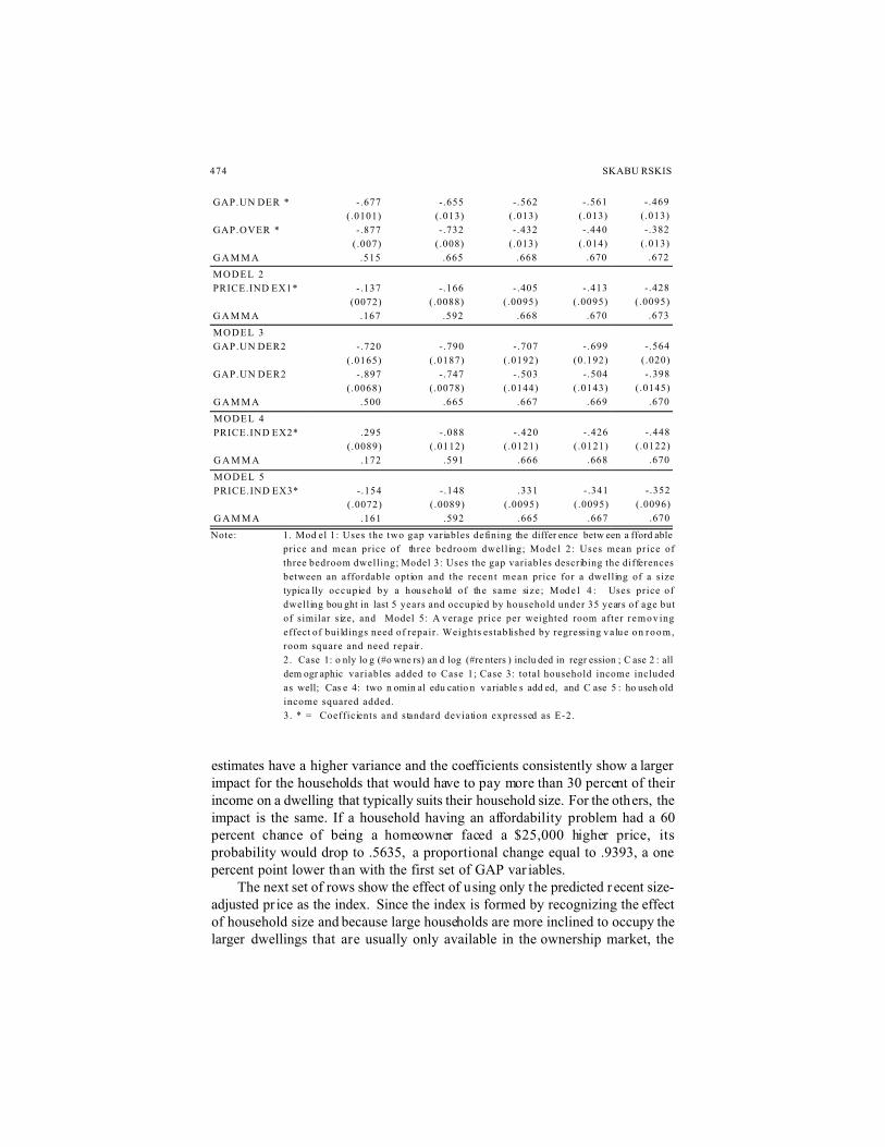
The four other indexes use an average value as the base but differ in themanner in which the size of the dwellings is standardised. Unlike with the GAPvariables, the coefficients for the alternative indexes increase in absolutemagnitude as the control variables are entered. The first alternative index is theone defined earlier and will be used in the next section. It is the average valueof three-bedroom owner-occupied dwellings and, when entered with all thecontrol variables, has an estimated coefficient of -.428 E-2 with a standarddeviation of .0095 E-2. This value is halfway between the coefficients for thetwo GAP variables. The Gamma statistic for the complete equation is .673,showing that this index yields a better fitting model than the one with the twoGAP variables. However, the GAP specification yields more interesting resultsfor the younger age groups because the effect of price varies depending onwhether it is above or below the household’s “affordable” level.
The second alternative recognises that the relevant index should measure thedistance between the “affordable” and the mean price of a dwelling that wouldtypically suit the household’s size. When holding income constant, small andlarge households face different burdens in buying and paying for housing. Theconstruction of this index also recognises that the relevant price, when lookingat the household’s current tenure status as opposed to its past tenure decisions,is the one revealed through recent transactions. It is the price renters would haveconsidered most recently when deciding not to make the decision that is, for themost part, irr eversible unless the household splits up or makes a long distancemove. The third set of rows in Table 5 show the coefficients for the two GAPvariables when they are constructed by using this construction of the relevantmarket price. The GAP variables move much like the first ones except that theTABLE 5 Estimated Coefficients and Their Standard Deviations for the GAP Va riables Using
Alternative Specifications
MODEL 1 Case 1 Case 2 Case 3 Case 4 Case 5
474 SKABU RSKIS
GAP.UN DER *
GAP.OVER *
G A M M A
-.677
(.0101)
-.877
(.007)
.515
-.655
(.013)
-.732
(.008)
.665
-.562
(.013)
-.432
(.013)
.668
-.561
(.013)
-.440
(.014)
.670
-.469
(.013)
-.382
(.013)
.672
MODEL 2
PRICE.IND EX1*
G A M M A
-.137
(0072)
.167
-.166
(.0088)
.592
-.405
(.0095)
.668
-.413
(.0095)
.670
-.428
(.0095)
.673
MODEL 3
GAP.UN DER2
GAP.UN DER2
G A M M A
-.720
(.0165)
-.897
(.0068)
.500
-.790
(.0187)
-.747
(.0078)
.665
-.707
(.0192)
-.503
(.0144)
.667
-.699
(0.192)
-.504
(.0143)
.669
-.564
(.020)
-.398
(.0145)
.670
MODEL 4
PRICE.IND EX2*
G A M M A
.295
(.0089)
.172
-.088
(.0112)
.591
-.420
(.0121)
.666
-.426
(.0121)
.668
-.448
(.0122)
.670
MODEL 5
PRICE.IND EX3*
G A M M A
-.154
(.0072)
.161
-.148
(.0089)
.592
.331
(.0095)
.665
-.341
(.0095)
.667
-.352
(.0096)
.670
Note: 1. Mod el 1: Uses the two gap variables defining the differ ence betw een a fford able
price and mean price of three bedroom dwelling; Mode l 2 : Uses mean price of
three bedroom dwelling; Model 3: Uses the gap variables describing the differences
between an affordable option and the recen t mean price for a dwelling of a size
typica lly occupied by a household of the same size; Mod e l 4 : Uses price of
dwelling bou ght in last 5 years and occupied by household under 35 years of age but
of similar size, and Model 5: A verage price per weighted room after r emov ing
effect of buildings need of repair. Weights established by regressing va lue on room,
room square and need repair.
2. Case 1: o nly lo g (#o wne rs) an d log (#re nters ) inclu ded in regr ession ; C ase 2 : all
dem ogr aphic variables added to Case 1; Case 3: total household income included
as well; Cas e 4: two n omin al edu catio n variable s add ed, and C ase 5 : ho useh old
income squared added.
3. * = Coefficients and standard deviation expressed as E-2.
estimates have a higher variance and the coefficients consistently show a largerimpact for the households that would have to pay more than 30 percent of theirincome on a dwelling that typically suits their household size. For the others, theimpact is the same. If a household having an affordability problem had a 60percent chance of being a homeowner faced a $25,000 higher price, itsprobability would drop to .5635, a proportional change equal to .9393, a onepercent point lower than with the first set of GAP var iables.
The next set of rows show the effect of using only the predicted r ecent size-adjusted pr ice as the index. Since the index is formed by recognizing the effectof household size and because large households are more inclined to occupy thelarger dwellings that are usually only available in the ownership market, the
HOUSING PRICES AND HOUSING DENSITY 475
24. Variants including categorical variables for e ach r oom and b edro om s ize did not y ield better
results.
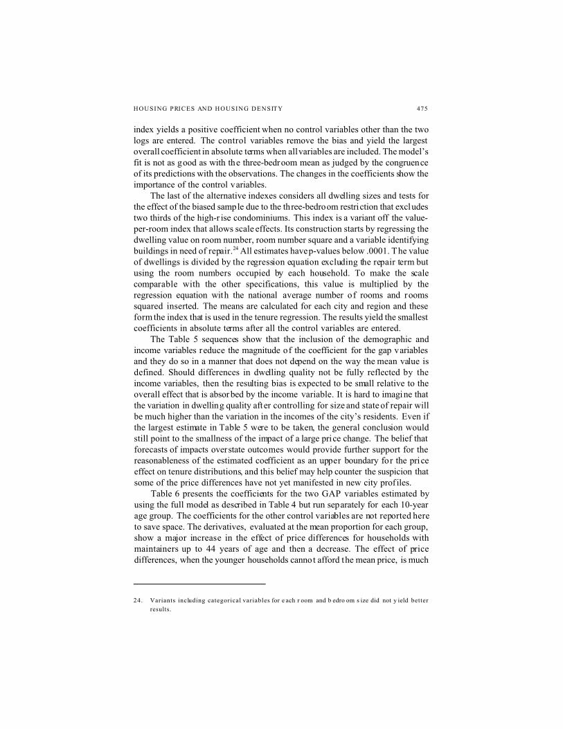
index yields a positive coefficient when no control variables other than the twologs are entered. The control variables remove the bias and yield the largestoverall coefficient in absolute terms when all variables are included. The model’sfit is not as good as with the three-bedroom mean as judged by the congruenceof its predictions with the observations. The changes in the coefficients show theimportance of the control variables.
The last of the alternative indexes considers all dwelling sizes and tests forthe effect of the biased sample due to the three-bedroom restriction that excludestwo thirds of the high-r ise condominiums. This index is a variant off the value-per-room index that allows scale effects. Its construction starts by regressing thedwelling value on room number, room number square and a variable identifyingbuildings in need of repair.24 All estimates have p-values below .0001. The valueof dwellings is divided by the regression equation excluding the repair term butusing the room numbers occupied by each household. To make the scalecomparable with the other specifications, this value is multiplied by theregression equation with the national average number of rooms and roomssquared inserted. The means are calculated for each city and region and theseform the index that is used in the tenure regression. The results yield the smallestcoefficients in absolute terms after all the control variables are entered.
The Table 5 sequences show that the inclusion of the demographic andincome variables reduce the magnitude of the coefficient for the gap variablesand they do so in a manner that does not depend on the way the mean value isdefined. Should differences in dwelling quality not be fully reflected by theincome variables, then the resulting bias is expected to be small relative to theoverall effect that is absor bed by the income variable. It is hard to imagine thatthe variation in dwelling quality after controlling for size and state of repair willbe much higher than the variation in the incomes of the city’s residents. Even ifthe largest estimate in Table 5 were to be taken, the general conclusion wouldstill point to the smallness of the impact of a large price change. The belief thatforecasts of impacts overstate outcomes would provide further support for thereasonableness of the estimated coefficient as an upper boundary for the priceeffect on tenure distributions, and this belief may help counter the suspicion thatsome of the price differences have not yet manifested in new city prof iles.
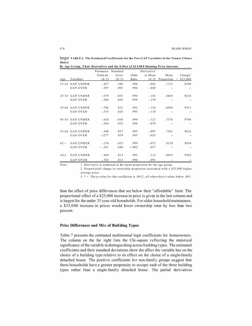
Table 6 presents the coefficients for the two GAP variables estimated byusing the full model as described in Table 4 but run separately for each 10-yearage group. The coefficients for the other control variables are not reported hereto save space. The derivatives, evaluated at the mean proportion for each group,show a major increase in the effect of price differences for households withmaintainers up to 44 years of age and then a decrease. The effect of pricedifferences, when the younger households cannot afford the mean price, is much
476 SKABU RSKIS
larger TABLE 6 The Estimated Coefficients for the Two GAP Variables in the Tenure Choice
Mod el
By Age G roup, T heir Derivatives and the E ffect of $2 5,00 0 Housing Pr ice Increase
Age Variables
Parameter
Estim ate
(E-2)
Standard
Error
(E-2)
Odds
Ratio
Derivative1
at Mean
(E-2)
Mean
Proportion
Change 2
+ $25,000
15-24 GAP.UNDER -.427 .106 .996 -.043 .1133 .9109
GAP.OVER -.397 .093 .996 -.040 -- --
25-34 GAP.UNDER -.579 .035 .994 -.143 .4445 .9216
GAP.OVER -.564 .026 .994 -.139 -- --
35-44 GAP.UNDER -.706 .033 .993 -.156 .6694 .9913
GAP.OVER -.535 .026 .995 -.118 -- --
45-54 GAP.UNDER -.626 .038 .994 -.121 .7376 .9706
GAP.OVER -.364 .032 .996 -.070 -- --
55-64 GAP.UNDER -.500 .037 .995 -.097 .7381 .9816
GAP.OVER -.127* .039 .995 -.025 -- --
65 + GAP.UNDER -.138 .023 .999 -.033 .6139 .9834
GAP.OVER + .241 .040 1.002 .057 -- --
ALL GAP.UNDER -.469 .013 .995 -.112 .6053 .9582
GAP.OVER -.382 .013 .996 -.091 -- --
Note: 1. Derivative is estimated at the mean proportion for the age group.
2. Proportional change in ownership proportion associated with a $25,000 higher
average price.
3. * = The p-value for this coefficient is .0012, all others have values below .001.
than the effect of price differ ences that are below their “affordable” limit. Thepropor tional effect of a $25,000 increase in price is given in the last column andis largest for the under 35 year-old households. For older household maintainers,a $25,000 increase in prices would lower ownership rates by less than twopercent.
Price Differences and Mix of Building Types
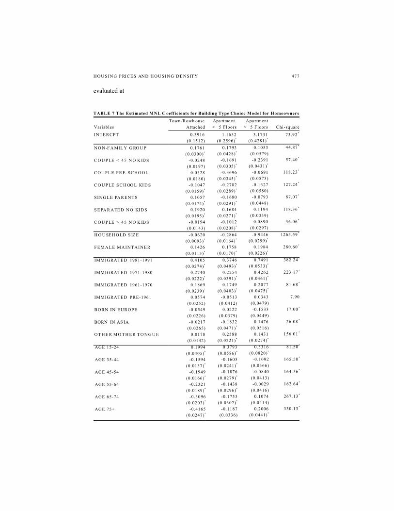
Table 7 presents the estimated multinomial logit coefficients for homeowners.The column on the far right l ists the Chi-square reflecting the statist icalsignificance of the variable in distinguishing across building types. The estimatedcoefficients and their standard deviations show the effect the variable has on thechoice of a building type relative to its effect on the choice of a single-familydetached house. The positive coefficients for non-family groups suggest thatthese households have a greater propensity to occupy each of the three buildingtypes rather than a single-family detached house. The partial derivatives
HOUSING PRICES AND HOUSING DENSITY 477
evaluated at
TABLE 7 The Estimated MNL C oefficients for Building Type Choice Model for Homeowners
Variables
Town /Rowh ouse
Attached
Apa rtme nt
< 5 Floors
Apartment
> 5 Floors Chi-square
INTERCPT 0.3916
(0.1512)
1.1632
(0.2596)*
3.1731
(0.4281)*
73.92 *
N O N -F A M IL Y G RO U P
C O U P LE < 4 5 N O K ID S
COUPLE PRE-SCHOOL
C O U P LE S C H OO L KI D S
SINGLE PARENTS
S E PA R A TE D N O KI D S
C O U P LE > 4 5 N O K ID S
0.1761
(0.0300)*
-0.0248
(0.0197)
-0.0528
(0.0180)
-0.1047
(0.0159)*
0.1057
(0.0174)*
0.1920
(0.0195)*
-0.0194
(0.0143)
0.1793
(0.0428)*
-0.1691
(0.0305)*
-0.3696
(0.0345)*
-0.2782
(0.0289)*
-0.1680
(0.0291)*
0.1684
(0.0271)*
-0.1012
(0.0208)*
0.1053
(0.0579)
-0.2391
(0.0431)*
-0.0691
(0.0573)
-0.1327
(0.0580)
-0.0793
(0.0448)
0.1194
(0.0339)
0.0890
(0.0297)
44.87 *
57.40 *
118.23 *
127.24 *
87.07 *
118.36 *
36.06 *
H O U SE H O LD S IZ E
FEMALE MAINTAINER
-0.0620
(0.0093)*
0.1426
(0.0113)*
-0.2864
(0.0164)*
0.1758
(0.0170)*
-0.9446
(0.0299)*
0.1984
(0.0226)*
1265.59 *
280.60 *
IMMIGRATED 1981-1991
IMMIGRATED 1971-1980
IMMIGRATED 1961-1970
IMMIGRATED PRE-1961
BORN IN EUROPE
BORN IN AS IA
O T H E R M O T H E R T O N G U E
0.4105
(0.0274)*
0.2740
(0.0222)*
0.1869
(0.0239)*
0.0574
(0.0252)
-0.0549
(0.0226)
-0.0217
(0.0265)
0.0178
(0.0142)
0.3746
(0.0493)*
0.2254
(0.0391)*
0.1749
(0.0403)*
-0.0513
(0.0412)
0.0222
(0.0379)
-0.1832
(0.0471)*
0.2588
(0.0221)*
0.7491
(0.0533)*
0.4262
(0.0461)*
0.2077
(0.0475)*
0.0343
(0.0479)
-0.1533
(0.0449)
0.1476
(0.0516)
0.1431
(0.0274)*
382.24 *
223.17 *
81.68 *
7.90
17.00 *
26.08 *
156.01 *
AGE 15-24
AGE 35-44
AGE 45-54
AGE 55-64
AGE 65-74
AGE 75+
0.1994
(0.0405)*
-0.1594
(0.0137)*
-0.1949
(0.0166)*
-0.2321
(0.0189)*
-0.3096
(0.0203)*
-0.4165
(0.0247)*
0.3793
(0.0586)*
-0.1603
(0.0241)*
-0.1876
(0.0279)*
-0.1438
(0.0296)*
-0.1753
(0.0307)*
-0.1187
(0.0336)
0.5316
(0.0820)*
-0.1092
(0.0366)
-0.0840
(0.0413)
-0.0029
(0.0416)
0.1074
(0.0414)
0.2006
(0.0441)*
81.50 *
165.50 *
164.56 *
162.64 *
267.13 *
330.13 *
478 SKABU RSKIS
25. The der ivat ive of the probabi li ty wi th respect to Xj is :
HIGH.SCHOOL
UNIVERSITY
-0.0310
(0.0106)
-0.0083
(0.0111)
-0.0937
(0.0164)*
0.0785
(0.0177)*
0.1606
(0.0239)*
0.0831
(0.0224)
91.57 *
33.85 *
TABLE 7 cont’d Estimated M NL Co efficients, Ho meow ners
I N C OM E
PRICE. INDEX
-0.0692
(0.0033)*
0.00144
(0.00024)*
-0.0878
(0.0055)*
0.00421
(0.00037)*
0.0274
(0.0060)*
0.00311
(0.00051)*
676.27 *
173.78 *
L O G (# S FD )
L O G (# T O WN )
LOG(#LO.APT)
LOG(#HI .APT)
-0.9161
(0.0254)*
0.9273
(0.0339)*
0.0378
(0.0096)*
-0.0225
(0.0167)
-1.3119
(0.0469)*
0.4729
(0.0647)*
1.0643
(0.0166)*
-0.2827
(0.0313)*
-1.0813
(0.0725)*
0.2429
(0.0846)
0.0575
(0.0210)
0.7929
(0.0489)*
2072.01 *
778.60 *
4114.67 *
355.90 *
Number of Cases: 133,594 80,474
Note: 1. * = p-value # .0000.
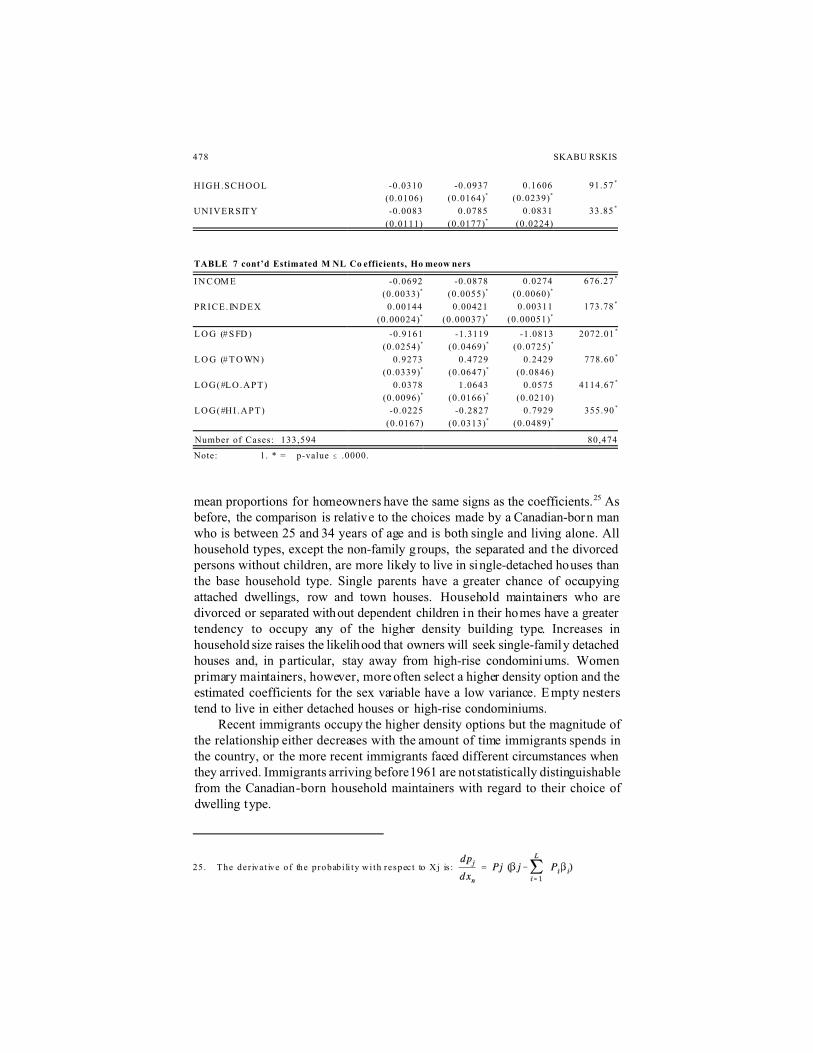
mean proportions for homeowners have the same signs as the coefficients.25 Asbefore, the comparison is relative to the choices made by a Canadian-born manwho is between 25 and 34 years of age and is both single and living alone. Allhousehold types, except the non-family groups, the separated and the divorcedpersons without children, are more likely to live in single-detached houses thanthe base household type. Single parents have a greater chance of occupyingattached dwellings, row and town houses. Household maintainers who aredivorced or separated without dependent children in their homes have a greatertendency to occupy any of the higher density building type. Increases inhousehold size raises the likelihood that owners will seek single-family detachedhouses and, in particular, stay away from high-rise condominiums. Womenprimary maintainers, however, more often select a higher density option and theestimated coefficients for the sex variable have a low variance. E mpty nesterstend to live in either detached houses or high-rise condominiums.
Recent immigrants occupy the higher density options but the magnitude ofthe relationship either decreases with the amount of time immigrants spends inthe country, or the more recent immigrants faced different circumstances whenthey arrived. Immigrants arriving before 1961 are not statistically distinguishablefrom the Canadian-born household maintainers with regard to their choice ofdwelling type.
HOUSING PRICES AND HOUSING DENSITY 479
26. This cross-sectional analysis shows the effect of price differences. The older age gro ups w ill
have gro wn u p in citie s with h igher price s and may , th erefore, have been kept out of
homeownership. Peo ple bu ying hom es in the higher priced cities may have been more inclined
to buy sma ller un its in more de nse building form s. Fo r ho meo wne rship , an incre ase in over all
price levels may make housing appear to be an even better investment than they expected. The
price increase may, therefore, stimulate the deman d for more housing, larger housing
investments and, thereby, encourag e homeo wners to seek single-family houses.
Both the youngest and oldest age group shows a tendency to live in high-r isecondominiums. The youngest, under 24, tend not to own detached houses.Households with maintainers between 25 and 55 have a greater tendency tooccupy detached houses than the base group. Maintainers over 54 years of ageare distinguished by prefer ring either houses or high-rise condominiums but notthe medium density options. 26 The income variable shows that higher incomehouseholds increase their propensity to live in ei ther detached houses or high-risecondominiums. The derivat ives evaluated at the mean proportions for the ownerpopulation, however, show that each $1000 increase in income raises theprobability of owning a house by .01160 and of owning a high-r isecondominium unit by only .00168.
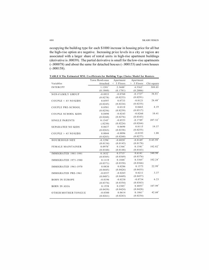
Table 8 presents the estimated coefficients for the renter’s choice of buildingtype. The general pat tern for renters is similar as that for owners in that increasesin household size are strongly related to the tendency to live in single-familydetached houses. Women primary maintainers, holding other factors constant,are more likely to choose one of the higher density options. The derivatives forthe age variables often have signs that differ from those of the est imatedcoefficients. A higher proportion of renters over 45 years of age live in high-riseapartments than the 25-34 year-olds that form the base and the older people areless frequently found in the other building types. The tendency to move to high-rise apartments in the higher priced regions starts after the age of 35!
The relationship between income and dwelling type differs in the rental andthe ownership sectors. The partial derivatives for the single family rental (.0003)and the town house (.0026) options are positive. The derivatives for low- and forhigh-rise apartments are -.0215 and . 0095 respectively when evaluated at therenters’ mean propor tion. Higher income households have a greater tendency tooccupy either high-rise apar tments or detached houses. The decrease in thechance of occupying a low-rise apartment unit may well be due to our inabilityto control for differences in building quality by using var iables other thanincome. Low-rise apartments, wood frame and without elevators, are among thelowest cost housing types in Canada. The income variable, however, does appearto help account for quality differences as a strong negative relationship wasfound for the income variable and the propensity to live in a low-rise apartment.
The price index yields positive coefficients for all building types but onlythe two for the low- and high-rise apartments are different from zero at areasonable p-level. The partial derivatives showing the change in probability of
480 SKABU RSKIS
occupying the building type for each $1000 increase in housing price for all butthe high-r ise option are negative. Increasing pr ice levels in a city or region areassociated with a larger share of rental units in high-rise apartment buildings(derivative is .00039). The partial derivative is small for the low-rise apartments(-.000078) and about the same for detached houses (-.000153) and town houses(-.000158).
TABLE 8 The Estimated MNL Co efficients for Building Type Choice Model for Renters
Variables
Town /Rowh ouse
Attached
Apartment
< 5 Floors
Apartment
> 5 Floors Chi-square
INTERCPT 1.1201 *
(0.1860)
2.3688 *
(0.1781)
4.5363 *
(0.2006)
589.05
N O N -F A M IL Y G RO U P
C O U P LE < 4 5 N O K ID S
COUPLE PRE-SCHOOL
C O U P LE S C H OO L KI D S
SINGLE PARENTS
S E PA R A TE D N O KI D S
C O U P LE > 4 5 N O K ID S
-0.0933
(0.0278)
0.0597
(0.0245)
0.0501
(0.0256)
0.0490
(0.0260)
0.1345 *
(.0230)
0.0637
(0.0263)
0.0044
(0.0283)
-0.0760
(0.0253)
0.0733
(0.0224)
0.0319
(0.0259)
-0.0243
(0.0276)
-0.0553
(0.0224)
0.0690
(0.0238)
-0.0096
(0.0260)
-0.1727 *
(0.0291)
-0.0121
(0.0255)
0.0463
(0.0317)
-0.0260
(0.0343)
-0.1749 *
(0.0264)
0.0115
(0.0255)
-0.0193
(0.0277)
36.81 *
26.48 *
4.19
10.41
207.32 *
19.37
1.08
H O U SE H O LD S IZ E
FEMALE MAINTAINER
-0.1296 *
(0.0134)
0.0970 *
(0.0160)
-0.6030 *
(0.0145)
0.1366 *
(0.0148)
-0.8149 *
(0.0178)
0.1541 *
(0.0163)
3145.99 *
102.82 *
IMMIGRATED 1981-1991
IMMIGRATED 1971-1980
IMMIGRATED 1961-1970
IMMIGRATED PRE-1961
BORN IN EUROPE
BORN IN AS IA
O T H E R M O T H E R T O N G U E
0.1832 *
(0.0385)
0.1119
(0.0371)
0.0830
(0.0445)
-0.0357
(0.0487)
-0.0196
(0.0374)
0.1558
(0.0439)
-0.0300
(0.0261)
0.3715 *
(0.0369)
0.1848 *
(0.0358)
0.0286
(0.0426)
-0.0265
(0.0449)
-0.0238
(0.0354)
0.2305 *
(0.0424)
0.0614
(0.0243)
0.6141 *
(0.0376)
0.3365 *
(0.0366)
0.1573
(0.0435)
0.0211
(0.0457)
-0.0734
(0.0363)
0.4053 *
(0.0428)
0.1061 *
(0.0254)
340.90 *
102.24 *
22.99 *
3.37
6.23
107.99 *
42.60 *
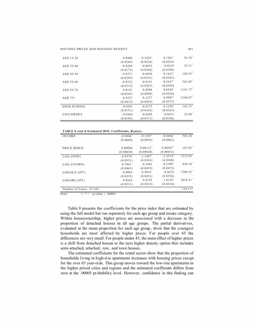
HOUSING PRICES AND HOUSING DENSITY 481
AGE 15-24
AGE 35-44
AGE 45-54
AGE 55-64
AGE 65-74
AGE 75+
0.0480
(0.0242)
-0.0208
(0.0173)
-0.0371
(0.0245)
-0.0312
(0.0312)
0.0141
(0.0342)
0.0227
(0.0413)
0.1456 *
(0.0224)
-0.0622
(0.0168)
-0.0458
(0.0233)
-0.0181
(0.0287)
0.0288
(0.0309)
0.1277
(0.0365)
0.1201 *
(0.0265)
0.0229
(0.0196)
0.1623 *
(0.0262)
0.3547 *
(0.0309)
0.6544 *
(0.0326)
0.9907 *
(0.0377)
56.76 *
35.31 *
120.53 *
362.65 *
1141.77 *
2140.67 *
HIGH.SCHOOL
UNIVERSITY
0.0243
(0.0151)
-0.0444
(0.0183)
-0.0173
(0.0143)
-0.0205
(0.0171)
0.1250 *
(0.0163)
0.0413
(0.0186)
142.33 *
32.89 *
TABLE 8 cont’d Estimated MNL Coefficients, Renters
I N C OM E
PRICE. INDEX
-0.0646 *
(0.0060)
0.00044
(0.00030)
-0.1267 *
(0.0058)
0.00112 *
(0.00028)
-0.0404 *
(0.0062)
0.00287 *
(0.00031)
562.28 *
107.02 *
L O G (# S FD )
L O G (# T O WN )
LOG(#LO.APT)
LOG(#HI .APT)
-0.8574 *
(0.0351)
0.7461 *
(0.0461)
0.0882
(0.0235)
0.0243
(0.0231)
-1.1447 *
(0.0343)
0.1062
(0.0455)
0.9916 *
(0.0221)
0.0755
(0.0215)
-1.2519 *
(0.0368)
0.2399 *
(0.0472)
-0.0272
(0.0236)
1.0129 *
(0.0234)
1312.03 *
438.18 *
7280.32 *
3618.51 *
Number of Cases: 87,102 139,177
Note: 1. * = p-value # .00001.
Table 9 presents the coefficients for the price index that are estimated byusing the full model but run separately for each age group and tenure category.Within homeownership, higher prices are associated with a decrease in theproportion of detached houses in all age groups. The partial derivatives,evaluated at the mean proportion for each age group, show that the youngesthouseholds are most affected by higher prices. For people over 65 thedifferences are very small. For people under 45, the main effect of higher pricesis a shift from detached houses to the next higher density option that includessemi-attached, attached, row, and town houses.
The estimated coefficients for the rental sector show that the proportion ofhouseholds l iving in high-rise apartments increases with housing prices exceptfor the over 65 year-olds. This group moves toward the low-rise apartments inthe higher priced cities and regions and the estimated coefficient differs fromzero at the .00005 probability level. However, confidence in this finding can
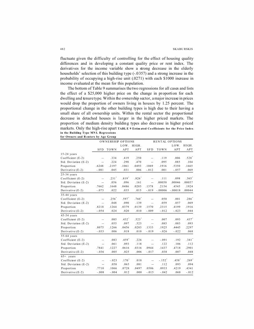
482 SKABU RSKIS
fluctuate given the difficulty of controlling for the effect of housing qualitydifferences and in developing a constant quality price or rent index. Thederivatives for the income variable show a strong decrease in the elderlyhouseholds’ selection of this building type (-.0357) and a strong increase in theprobability of occupying a high-rise unit (.0271) with each $1000 increase inincome evaluated at the mean for this population.
The bottom of Table 9 summarises the two regressions for all cases and liststhe effect of a $25,000 higher price on the change in proportion for eachdwelling and tenure type. Within the ownership sector, a major increase in priceswould drop the proportion of owners living in houses by 1.25 percent. Theproportional change in the other building types is high due to their having asmall share of all ownership units. Within the rental sector the proportionaldecrease in detached houses is larger in the higher priced markets. Theproportion of medium density building types also decrease in higher pricedmarkets. Only the high-rise apart TABL E 9 Estim ated Co efficients for the Price Index
in the Building Type MN L Regressions
for Owners and R enters by Age Group
O W N E RS H IP O P TI O NS R E N T AL O P TI O NS
S F D T O W N
L O W .
APT
H I GH .
APT S F D T O W N
L O W .
APT
H I GH .
APT
15-24 years
Coefficient (E-2) -- .334 .419 .250 -- .119 .006 .528 *
Std. Deviation (E-2) -- .224 .298 .470 -- .095 .085 .104
Proportion .6248 .2197 .1061 .0493 .1069 .1916 .5350 .1665
Derivative (E-2) -.081 .045 .031 .006 -.012 .001 -.057 .069
25-34 years
Coefficient (E-2) -- .231 * .819 * .826 * -- .111 .098 .365 *
Std. Deviation (E-2) -- .056 .096 .161 -- .00050 .00046 .00057
Proportion .7662 .1648 .0486 .0203 .1378 .2154 .4545 .1924
Derivative (E-2) -.073 .022 .035 .015 -.019 -.00006 -.00018 .00044
35-44 years
Coefficient (E-2) -- .256 * .597 * .760 * -- .050 .001 .286 *
Std. Deviation (E-2) -- .048 .090 .139 -- .059 .057 .069
Proportion .8218 .1264 .0379 .0139 .1570 .2315 .4199 .1916
Derivative (E-2) -.054 .024 .020 .010 -.009 -.012 -.023 .044
45-54 years
Coefficient (E-2) -- .085 .432 * .523 * -- .007 .093 .437 *
Std. Deviation (E-2) -- .055 .097 .523 -- .085 .083 .093
Proportion .8075 .1266 .0456 .0203 .1333 .1925 .4445 .2297
Derivative (E-2) -.033 .006 .018 .010 -.019 -.026 -.022 .068
55-64 years
Coefficient (E-2) -- .083 .459 * .226 -- -.091 .192 .341 *
Std. Deviation (E-2) -- .061 .093 .118 -- .122 .106 .112
Proportion .7841 .1227 .0616 .0316 .0944 .1437 .4718 .2901
Derivative (E-2) -.036 .005 .025 .006 -.017 .038 .007 .048
65+ years
Coefficient (E-2) -- -.023 .170 * .018 -- -.152 * .458 * .269 *
Std. Deviation (E-2) -- .058 .065 .081 -- .112 .093 .094
Proportion .7710 .1066 .0728 .0497 .0506 .0933 .4219 .4341
Derivative (E-2) -.008 -.004 .012 .000 -.015 -.042 .068 -.012
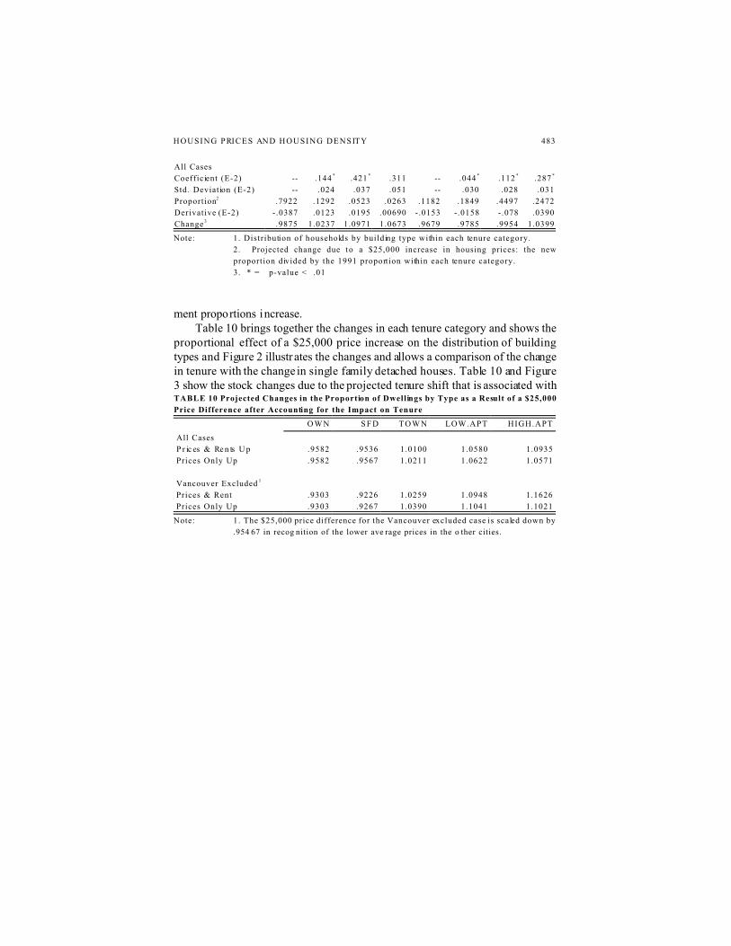
HOUSING PRICES AND HOUSING DENSITY 483
All Cases
Coefficient (E-2) -- .144 * .421 * .311 -- .044 * .112 * .287 *
Std. Deviation (E-2) -- .024 .037 .051 -- .030 .028 .031
Proportion2 .7922 .1292 .0523 .0263 .1182 .1849 .4497 .2472
Derivative (E-2) -.0387 .0123 .0195 .00690 -.0153 -.0158 -.078 .0390
Change 3 .9875 1.0237 1.0971 1.0673 .9679 .9785 .9954 1.0399
Note: 1. Distribution of households by building type within each tenure category.
2. Projected change due to a $25,000 increase in housing prices: the new
proportion divided by the 1991 proportion within each tenure category.
3. * = p-value < .01
ment proportions increase.Table 10 brings together the changes in each tenure category and shows the
proportional effect of a $25,000 price increase on the distribution of buildingtypes and Figure 2 illustr ates the changes and allows a comparison of the changein tenure with the change in single family detached houses. Table 10 and Figure3 show the stock changes due to the projected tenure shift that is associated withTABLE 10 Projected Changes in the Proportion of Dwellings by Type as a Result of a $25,000
Price Difference after Accounting for the Impact on Tenure
O W N S F D T O W N LOW.APT HIGH.APT
All Cases
P r ic es & Re n ts U p .9582 .9536 1.0100 1.0580 1.0935
Prices Only Up .9582 .9567 1.0211 1.0622 1.0571
Vancouver Excluded 1
Prices & Rent
Prices Only Up
.9303
.9303
.9226
.9267
1.0259
1.0390
1.0948
1.1041
1.1626
1.1021
Note: 1. The $25,000 price difference for the Vancouver excluded case is scaled down by
.954 67 in recog nition of the lower ave rage prices in the o ther cities.
484 SKABU RSKIS
27. Estimates using one M NL mod el with the eight categories of building and tenure type gave
the same ratio for detached houses ( . 9591) bu t lowe r ratio s for th e cha nge in own ersh ip
(.9873) and much lower for th e lo w- and h igh- r ise apar tments (1 .0201 ,1 .0175). The town
house option increased b y 1.0 817 wh en using the single eq uation mod el. Tests f or th e IIA
assumption could not be performed with the available software and the large size of the
variance/c ovariance m atrix for the coefficients. However, the low er ra tio for the ow ners hip
options is most likely due to the char acter istics tha t give c omm on v alue to each optio n with in
the set of ow ners hip options are not being identified by the coefficients. The bias is expected
to understate the effect of the shar e of value of all the hom eownersh ip options.
FIGURE 2 Proportional Change in Building Types and in Ownership as a Result of a $25,000
Increase in Housing Proce Level, 1991FIGURE 3 Changes in the Size of the Stock as a Result of the Effect of a $25,000 Price
Increase on Home-Ownership Rates
$25000 higher house prices. The first row uses the results from both regressionsand implicitly assumes that a price increase in the ownership sector has acorresponding impact in the rental market. The second row accepts that rentsmay not change at all as a result of increases in ownership prices and shows thepropor tional effects on the total stock of a change in ownership prices. Thedecline in the proportion of detached houses is less than five percent and theratio is hardly affected by changes in rent.27
Conclusions

HOUSING PRICES AND HOUSING DENSITY 485
The estimates developed in this study related price differences with differencesin tenure and building type as they were seen in 1991. Two qualifications areneeded when using the coefficients to predict the effect of future price changes.First, the structural relationships may change to mitigate some of theconsequences of rising prices. Second, the markets may not have been inequilibrium and recent price changes may have caused the estimated coefficientsto describe the short- rather than the long-run effects.
Dramatic but erroneous predictions have been made of the housing pr iceeffects of changing demographic profiles. Housing markets are complex withnew aspects being discovered after past predictions fail to be realised. Theobserved changes are often smaller than the predicted changes as the Skaburskis-Teitz (2001) conjecture suggests: “F orecasts overstate outcomes” .
Housing price increases should reduce housing consumption and keep peoplein rental tenure as standard economic theory would predict. However, somepeople will not stay as renters after a price increase but will change theirresponse patterns to put themselves into pover ty to buy a home as illustrated byBourassa (1996). The increase in the role of gifts is another example of adiscovery made after observed behaviour differed from predictions based onprevious empirical work. This is not to say that the previous models wereinadequately specified but that social systems appear homeostatic to a degreewith behavioral changes dampening the effects of changes in key var iables. Afterall, the quest for home ownership and the house with a yard is an entrenchedgoal for most North Americans and a desired state for most people in the world.
While mitigating factors may emerge to reduce the impacts of price changes,the prolonged effect of a price increase may have more of an effect on dwellingtype than indicated by the coefficients presented here. Housing markets inCanada were remarkably stable during the 1980s, except for Vancouver, andmight reasonably be thought of as being in equilibrium. However, immigrationto Vancouver and the lower mainland in British Columbia led to rapid pr iceinflation starting in 1989 and continuing through the early 1990s. Removing theVancovuer cases from the analysis leaves the stable, slow growing cities in thesample and results in considerably larger coefficients for both the tenure and thebuilding type equations. The net effect is illustrated by the bottom two rows inTable 10. The projected impact of a major price increase that persists over thelong run may be considerably larger than the one predicted by the estimatedcoefficients.
Given the two sources of errors, what then is the likely effect of a $25,000increase in housing price levels? A safe guess would be a five percent reductionin the proportion of single-family houses. If no other mechanisms emerge tomediate the impact, then a larger decline is expected, perhaps as large as eightpercent. For people in the 25-45 age group the impact may be as high as 10percent. The reduction in single-family houses is primarily due to a reduction inthe number of young households that enter homeownership. The changes withinthe homeownership sector itself are small. Moreover, the reduction in the growth
486 SKABU RSKIS
of single-family houses in response to a price increase would not occur if othergovernment programs are initiated to stimulate homeownership among youngpeople. A policy of using development exactions to reduce demand for single-family houses would counter the goals embedded in programs that promote homeownership. Policies that limit growth in cities at the expense of increasinghousing price may make cities more livable, but at the expense of making theNorth American dream of homeownership fade further into the distance foryoung people.
References
Alonso, W. 1964. Location and Land Use. Cambridge: Harvard UniversityPress.
Arnott, R.J. 1980. “ A Simple Urban Growth Model with Durable Housing”.Journal of Regional Science and Urban Economics , 10: 53-76.
Artle, R. and P. Varaiya. 1978. “ Life Cycle Consumption and Homeownership”. Journal of Economic Theory, 18: 38-58.
Börsch-Supan, A. and J. Pitkin. 1988. “ On Discrete Choice Models of HousingDemand”. Journal of Urban Economics, 24: 153-172.
Bourassa, S.C. 1994. “ Immigration and Housing Tenure Choice in Austral ia” .Journal of Housing Research, 5: 117-137.
_______. 1995. “ The Impacts of Borrowing Constraints on Home-Ownershipin Austral ia” . Urban Studies, 32: 1163-1173.
_______. 1995. “ A Model of Housing Tenure Choice in Australia” . Journal ofUrban Economics , 37: 161-175.
_______. 1996. “Measuring the Affordabil ity of Home ownership”. UrbanStudies, 33: 1867-1877.
Brueckner, J. 1986. “The Downpayment Constraint and Housing TenureChoice: A Simplified Exposition”. Journal of Regional Science and UrbanEconomics, 16: 519-525.
Cho, C. -J. 1997. “Joint Choice of Tenure and Dwelling Type: A MultinomialLogit Analysis for the City of Chongju”. Journal of Urban Studies, 34:1459-1473.
Cooperstein, R.L. 1989. “Quantifying the Decision to Become a First-TimeHome Buyer”. Urban Studies, 26: 223-233.
Engelhardt, G.V. 1994. “House Prices and the Decision to Save for Downpay-ments”. Journal of Urban Economics. 36: 209-237.
Engelhardt, G.V. and C.J. Mayer. 1994. “Gifts for Home Purchase andHousing Market Behaviour”. New England Economic Review, May/June:47-58.
_______. 1998. “ Intergenerational Transfers, Borrowing Constraints, andSaving Behaviour: Evidence from the Housing Market”. Journal of UrbanEconomics, 44: 135-157.
HOUSING PRICES AND HOUSING DENSITY 487
Fortin. N.M. 1995. “ Allocation Inflexibilities, Female Labour Supply, andHousing Assets Accumulation: Are Women Working to Pay the Mortgage?”Journal of Labour Economics , 13: 524-557.
Haurin, D.R. , P. H. Hendershott and S.M. Wachter. 1996. “ WealthAccumulation and Housing Choices of Young Households”. Journal ofHousing Research , 7: 33-58.
Henderson, J. V. and Y.M. Ioannides. 1989a. “Dynamic Aspects of ConsumerDecision in Housing Markets”. Journal of Urban Economics, 26: 212-230.
_______. 1989b. “ The Impact of Borrowing Constraints on Home Ownership”.AREUEA Journal, 17: 389-402.
Jones, L.D. 1989. “Current Wealth and Tenure Choice” . Journal of theAmerican Real Estate and Urban Economics Association, 17: 17-40.
Kendig, H.L . 1984. “Housing Careers, Life Cycle and Residential Mobility:Implications for the Housing Market”. Urban Studies,. 21: 271-283.
Kim, S.-J. 1992. “ A Model of Rental Housing Choices in the Korean Market”.Urban Studies, 29: 1247-1264.
Linneman, P.D. and S. Wachter. 1989. “The Impact of Borrowing Constraintson Homeownership”. AREUEA Journal, 17: 389-402.
Linneman, P.D . and I.F . Megbolugbe. 1992. “ Housing Affordability: Myth orReality?” . Urban Studies, 29: 369-392.
Mayer, C. and G. V. Engelhardt. 1996. “ Gifts Downpayments, and HousingAffordability”. Journal of Housing Research, 7: 59-77.
McFadden, D. 1978. “Modelling the Choice of Residential Location”, in A.Karlqvist, L. Lundqvist, F. Snickers and J.W. Weibull (eds. ). Spatial Inter-action Theory and Planning Models. Amsterdam: North Holland.
Megbolugbe, I.F. and P. D. Linneman. 1993. “Home Ownership”. Journal ofUrban Studies, 30: 659-682.
Mulder, C.H. and M. Wagner. 1998. “F irst-Time Homeownership in theFamily Life Course: A West German-Dutch Comparison”. Urban Studies,35: 687-713.
Muth, R. 1969. Cities and Housing. Chicago: University of Chicago Press.Quigley, J.M. 1973. “ Estimates of a More General Model of Consumer Choice
in the Housing Markets”, in R.E. Grierson (ed.). The Urban Economy andHousing. Lexington: Lexington Books.
_______. 1976. “ Housing Demand in the Short Run: an Analysis of PolytomousChoice” . Explorations in Economic Research , 3: 76-102.
Ray, B. and E. M oore. 1991. “Access to Homeownership Among ImmigrantGroups in Canada” . Canadian Review of Sociology and Anthropology, 28:1-29.
Singell, L.D. and J.H. Lillydahl. 1990. “An Empirical Examination of theEffect of Impact Fees on the Housing Market”. Land Economics , 66: 82-92.
Skaburskis, A. 1990. “The Burden of Development Impact Fees” . LandDevelopment Studies, 7: 173-185.
_______. 1991. “The Design of Development Cost Charges”. Journal of
488 SKABU RSKIS
Property Research, 8: 83-98._______. 1994. “The Determinants of Canadian Headship Rates”. Urban
Studies, 31: 1377-1390._______. 1996. “Race and Tenure in Toronto” . Urban Studies, 31: 1377-1389._______. 1997. “ Gender Differences in Housing Demand”. Urban Studies, 34:
274-320.Skaburskis, A and M. Teitz. 2001. “Forecasts and Outcomes”. Forthcoming.Skaburskis, A. and M. Qadeer. 1992. “ Empirical Estimation of the Price Effects
of Development Impact Fees” . Urban Studies, 29: 651-666.Taylor, J. and R. Jureidini. 1994. “ The Implicit Male Norm in Australian
Housing F inance” . Journal of Economic Issues, 28: 543-554.Withers, D.S. 1998. “Linking Household Tr ansitions and Housing Tr ansitions:
A Longitudinal Analysis of Renters” . Environment and Planning A, 30:615-630.
Yates, J. 1998. “Is Australia’s Home Ownership Rate Really Stable? AnExamination of Change Between 1975 and 1994”. Urban Studies.(forthcoming).