HOW ARE ELECTRICITY PRICES SET IN AUSTRALIA?

Electricity prices faced by Australian households and small businesses are highly regulated. In states connected to the National Electricity Market (NEM) – New South Wales, Victoria, Queensland, South Australia and Tasmania – this is achieved through a combination of state and federal regulation. Western Australia is not part of the NEM and has its own system of regulation. This note outlines the processes by which end-user prices are set in the NEM states.

Forthcoming notes will discuss recent developments in utilities prices (Brown and Rosewall, 2010) and the drivers of recent price movements (Davis, 2010).

The appendix contains an overview of how the electricity market actually works, in terms of electricity flows and the various payments involved.

Retail price regulation

Electricity retailers are those businesses that sell electricity directly to the general public. The prices they can charge households and small businesses are limited by price controls imposed by state regulators (except in Victoria, which removed its retail price controls in 2009). The prices are set so that electricity retailers can recover what the state regulator deems to be the costs an ‘efficient’ retailer would expect to incur in the period for which the cap applies. Each electricity retailer must submit an application to the state regulator outlining its expected costs for the period ahead. The regulator has the discretion to amend the proposed costs if it does not believe they accurately reflect future costs or they have not been calculated correctly. As well as recovering these costs, retailers are allowed to make a ‘reasonable’ margin – ranging from 3 to 10 per cent, depending on the state.

Retail regulations cover one-year periods in Queensland and South Australia, and a three-year period in New South Wales.

The costs faced by electricity retailers – which implicitly determine retail electricity prices – broadly fall into three categories:

• retail operation costs, such as meter reading, billing, marketing etc.

• network costs

• wholesale electricity costs

Though it varies somewhat, the retail component typically makes up around 10 per cent of total costs, while the network and wholesale electricity costs each make up around 45 per cent. The diagram below outlines some of the key features of each of these costs. The remainder of this note focuses on network and wholesale electricity costs.

Electricity retailer costs

Retail operation costs

• Reset every 1-3 years

• Includes customer acquisition and retention; billing; meter reading etc.

Wholesale electricity costs

• Determined every 5 minutes

• Set in the National Electricity Market

• Price cap exists, but is rarely binding

Network costs

• Reset every 5 years

• Network revenues capped by the Australian Energy Regulator

10% 45% 45%

Network costs

When discussing electricity markets, the ‘network’ can be broken into two distinct parts:

• The transmission network takes electricity directly from the generators on high-voltage power lines and includes linkages across state borders.

• The distribution network comprises lower-voltage power lines, providing the link from the transmission network to the end customer.1

Transmission charges make up about 10 per cent of retail prices, while distribution charges make up about 35 to 50 per cent. Both are very capital intensive and typically only one transmission and distribution network service a given area, giving rise to geographical monopolies. As such, governments impose significant regulation on these networks.

Since 2005, the transmission networks in the NEM states have been regulated by the Australian Energy Regulator (AER).2,3

Regulation of distribution networks was previously undertaken by state agencies, but has been the responsibility of the AER since 2008. Due to historical differences, the exact type of regulation varies between distribution networks, but is typically either some form of price or revenue cap. The procedures for determining the relevant 5-year cap are similar to those described for transmission networks.

The AER sets 5-year revenue caps based on expected costs during that period. The regulatory process takes around 13 months and begins with a transmission network submitting a revenue proposal to the AER, including a pricing formula to allocate where that revenue is generated. The AER publishes a draft determination within six months, on which written submissions are invited over a period of at least 1½ months. The AER must then publish its final determination at least two months before the new regulatory period begins.

The AER’s decision is based on the amount of revenue that would reasonably be required to recover a set of costs, which are outlined in the National Electricity Rules. These costs are:

• Operational and maintenance expenditure, such as wages and rents

• A return on capital (which is affected by capital expenditure)

• Asset depreciation costs

• Tax liabilities

Though it varies by network, the available evidence is that the return on capital is typically the largest component for both transmission and distribution networks.

The return on capital

There are two main steps involved in determining the revenue allowed as ‘return on capital’. The first is to calculate the ‘regulated asset base’ (RAB) for each year within the regulatory period. This is achieved by determining the stock of network assets at the

1 Transmission and distribution networks in New South Wales, Queensland and Tasmania are owned by the state governments. In South Australia there is a mix of public and private ownership, while the Victorian networks and the state interconnectors are privately owned.

2 Prior to that, regulation was carried out by the Australian Consumer and Competition Commission (ACCC).

3 The AER is a separate legal entity with a board that reports to the ACCC. One of its board members must be an ACCC commissioner. It makes decisions under the National Electricity Law and National Electricity Rules.

start of the period, and rolling this forward year by year, adjusting for depreciation (which lowers the RAB), CPI inflation and expected capital expenditure in that year (which increase the RAB). Note that this ‘rolling’ approach implicitly values assets at their inflation adjusted construction cost, less depreciation.

The second step is to apply a ‘Weighted Average Cost of Capital’ (WACC) to the asset base at the start of each year. The WACC is what the regulator considers to be a commercial return on capital. How it is determined is discussed in more detail below, but the most recent determinations use figures of 9.72 and 9.76 per cent.

As an example of how this process works, consider a network with an initial asset base of $100, and a WACC of 10 per cent. This would allow the network to have ‘return on capital’ revenues of $10 in the first year. Now assume net capital expenditure (less depreciation) of $20 in that year and zero inflation. This is added to the initial asset base to determine the asset base in year two of $120. Applying the WACC, the network could make $12 revenue for a return on capital in year two. And so on.

Capital expenditure is an important driver of a networks’ asset base, and so the AER approves a capital expenditure profile for the 5-year control period. It is important to emphasise, however, that the revenue the AER allows to offset capital costs does not cover the entire capital expenditure in that year. Instead, it covers the allowable return on capital, which is determined by applying the WACC to the asset base. So it is the return on capital, not capital expenditure itself, which is factored into networks’ prices.

The ‘Weighted Average Cost of Capital’

The WACC is calculated by the AER at the beginning of each regulatory control period. It is essentially a weighted average of the return on equity and cost of debt, as determined by the AER. It consists of five main parts:

Gearing ratio Set at 0.6. This is used as the weight given to the cost of debt in the WACC.

Nominal risk-free rate Determined by the yield on 10-year CGS calculated shortly before the regulatory control comes into force – the period over which this is taken appears variable, with examples ranging from 15 to 40 business days.

Debt risk premium Determined by the spread on 10-year BBB+ rated corporate bonds.

Market risk premium Set at 6.5 per cent in the most recent parameter review.

Equity beta Set at 0.8 in the most recent parameter review.

The WACC is determined as follows:

WACC = gearing ratio * (nominal risk-free rate + debt risk premium) + (1 - gearing ratio) * (nominal risk-free rate + market risk premium * equity beta)

= NRFR + 0.6 * debt risk premium + 0.4 * 0.065 * 0.8

Thus, excepting reviews to the parameters (the last of which was conducted in May 2009), only movements in the yield on 10-year CGS and BBB+ rated corporate bonds will change the WACC. As the regulatory control periods are for 5 years, and the WACC is not recalculated during that period, it is possible for these to have changed considerably in that time, or for the methodology to have changed. This potentially creates large

adjustments in the first year of the next regulatory period. There is some evidence that this has occurred in the latest round of distribution network determinations.4

Wholesale electricity costs

The National Energy Market is the wholesale market from which electricity is purchased by electricity retailers (except in Western Australia and the Northern Territory). Unlike other aspects of electricity provision, it is generally considered to be quite competitive and prices are mostly unregulated. A price cap exists, but it is quite high and typically binds only a few times during the year when demand is at its peak.

Prices in the NEM are determined every five minutes, and averaged over each half hour period to get a spot price. Generators bid how much electricity they are willing to provide, and at what price, for each five minute interval. The Australian Electricity Market Operator (AEMO) then accepts the bids – starting from the lowest priced bid – up to the point where supply equals demand in that interval.5

Because wholesale prices are set by the market, but retail prices are regulated for the next 12 to 36 months, state regulators must estimate the cost of wholesale electricity that will be faced. Though the approach varies by state, this is typically achieved by estimating both the long run marginal cost (LRMC) of generation, and an expected ‘market price’ for electricity. Outside consultants often seem to be commissioned to produce these estimates.

The price paid for all electricity in those five minutes is that of the highest bid accepted. Electricity retailers typically enter into a variety of futures contracts to limit their exposure to significant price swings.

The LRMC is based on the price that would be charged by a theoretical system of generators which is designed to meet the retailer’s energy requirements at the least cost. That is, the mix of generators that is selected does not necessarily reflect the actual mix of generators in the market – it will vary as relative fuel costs change and some forms of power generation become relatively cheaper. Thus, the LRMC is affected by changes in fuel costs, changes in technology, improvements in operational efficiency and changes in the cost of building new generators.

The approach to determining the ‘market price’ that retailers are expected to face varies a bit by state, but generally involves consideration of expected spot prices in the NEM and possible contract arrangements. The process is complicated, but it essentially tries to determine the total cost an ‘efficient’ retailer would face in sourcing their electricity requirements if they used an optimal combination of purchasing from the spot market and using contracts to hedge against large price movements.

In NSW, the greater of the LRMC and expected market price is used as the energy cost allowance. In QLD, they are given equal weights.

George Gardner 6 July 2010

4 The WACC used for distribution networks reportedly increased by 126 basis points from the previous control period for Queensland and by 80 basis points for South Australia. For NSW, the risk-free rate fell by 116 basis points between the issuing of a draft and final determination. Considering that the total starting asset base for NSW and QLD distribution networks is over $15 billion in each state, and around $2¾ billion in SA, these variations in the WACC are non-trivial.

5 AEMO is an amalgamation of six electricity and gas industry bodies, created by the Council of Australian Governments. Membership is split 60/40 between government and industry, with fees charged on a cost-recovery basis. AEMO manages the day-to-day operation of the NEM and has a role in longer term planning of transmission networks and other market infrastructure.

Appendix: Getting electricity from A to B There are a number of players involved in getting electricity from the power station to the end consumer. The diagram below provides a simplified illustration of how this happens and the flow of funds that pay for it.6

The generators send electricity, purchased by electricity retailers from the NEM, to distribution points via the long-distance transmission network. The electricity then travels through the poles-and-lines distribution network directly to the end customer. Note that some large, energy intensive companies purchase directly from the NEM. Generators and electricity retailers sell/buy directly into/from the NEM at the spot price, and settlement occurs through the AEMO. While all transactions are undertaken at the spot price, there is significant use of OTC and traded derivative instruments in order to hedge against spot market price fluctuations. The retailer, as well as purchasing the electricity from the NEM, also pays access fees to the networks for use of their infrastructure. Ultimately the end-user pays for it all through their regular electricity bill.

6 In reality, retailers could have customers on more than one distribution network, and more than one transmission network may be involved. There are also complications to do with electricity trading between states.

National Electricity Market

Retailer

Generators

Select large consumer (e.g. aluminium smelter)

End-users

Retailer Transmission network

Distribution network

Distribution network

End-users

Electricity bill

Hedging contract payments – both OTC and SFE traded contracts used

Network access fees

Electricity spot price

Electricity spot price

Electricity spot price

Electricity flow

Money flow

The Price of Power: Recent Drivers of Retail Electricity Prices

Electricity prices rose by 18 per cent over the year to June 2010 and recent regulatory decisions suggest a further increase of a little over 10 per cent by June 2011 (Graph 1). This note investigates the factors driving price increases this year and over the next few years. For details about longer-run developments in utilities prices see Brown, Davis and Plumb (2010, forthcoming) and for details on how electricity prices are set see Gardner (2010).

Electricity price increases are largely being driven by rising network charges, reflecting the need to expand network capacity, replace ageing assets, meet higher reliability standards and cover higher input and borrowing costs. Network charges in Queensland are also being adjusted to pass through to customer excess costs incurred in previous periods; while, in contrast, network charges may fall next year in Victoria as excess revenues are passed back to customers. Wholesale energy costs are also rising, although to a lesser extent and the picture is somewhat mixed across states.

Key drivers of recent and expected price increases

Retail electricity prices (that is, prices for households and small businesses) are highly regulated. While retail customers are free to choose their electricity provider, all states (except Victoria) provide a regulated ‘standard contract price’.1

Graph 1

This price is set to allow retailers to cover three sets of costs: the costs associated with buying electricity from the wholesale market; ‘network’ costs – the costs associated with transmitting and distributing electricity from generators to end-users; and retail costs (such as marketing and billing) and a retail margin. The weight given to each component in overall retail prices varies somewhat, but generally the wholesale and network cost components each account for around 45 per cent of the total retail price, while retail costs and margins make up the remaining 10 per cent (Table 1).

-5

0

5

10

15

1993 1996 1999 2002 2005 2008 2011-5

0

5

10

15

Electricity Price Inflation*Year ended

% %Forecasts**

* The spike in 2000/01 reflects the introduction of the GST** Based on regulatory decisionsSources: ABS; RBA

The increases in regulated retail electricity prices over the next few years are primarily driven by higher network costs. Wholesale energy costs have also risen, although more modestly (particularly in NSW). The rest of this note investigates the factors driving the increases in these two components.

Table 1: Retail Electricity Price Increase

Percentage point contribution to annual average increase, nominal

Weight Energy

Australia Integral Energy

Country Energy

Queensland Retailers

NSW, 2010/11 – 2012/13 QLD, 2010/11

Network charges ~ 45 9.4 5.1 10.5 8.2

Generation/wholesale energy costs ~ 45 0.3 0.3 1.0 3.8

Retail costs & margins ~ 10 1.0 0.7 1.0 1.3

Total price increase (per cent) 10.8 6.3 12.4 13.3 Sources: IPART; QCA; RBA

Network costs

The network charges component of retail electricity prices is set at a national level (by the Australian Energy Regulator, AER) for each electricity distributor or transmitter connected to the National Electricity Market (NEM).2

1 In addition to the standard contract price, retailers may also offer discount plans or higher priced plans for additional features (such as wind or solar power).

It is based on the amount of revenue required to cover a network provider’s costs over a five year ‘regulatory control’ period. A new regulatory control

2 Western Australia is not part of the national electricity market. While retail prices are no longer regulated in Victoria, Victorian network charges are regulated by the AER.

2 period began (or will begin) in 2009/10 for NSW, 2010/11 for Queensland and South Australia and 2011 for Victoria. The costs considered include: operational and maintenance expenditure, a return on capital, asset depreciation costs and tax liabilities. The revenue requirement in each year does not aim to cover the total cost of capital expenditure incurred in that year; network providers are expected to borrow or use internal funds to finance this investment. Rather, the revenue requirement includes a ‘return on capital’ (which takes into account borrowing costs) and ‘regulatory depreciation’ (through which firms recoup the cost of capital expenditure over the life of an asset). The return on capital is typically the largest component of the revenue requirement and is calculated as the stock of physical network assets (called the regulatory asset base or RAB) multiplied by the weighted average cost of capital (WACC). The regulatory asset base is assumed to grow from year to year by the amount of net capital expenditure (adjusted for inflation). Therefore, for a given WACC, higher capital expenditure leads to a higher return on capital and, in subsequent years, a larger value for the depreciation term – both of these increase revenue requirements. Annual revenue requirements are smoothed over the regulatory control period and combined with forecasts of demand to determine the annual increase in network charges faced by customers. For a comprehensive explanation see Gardner (2010).

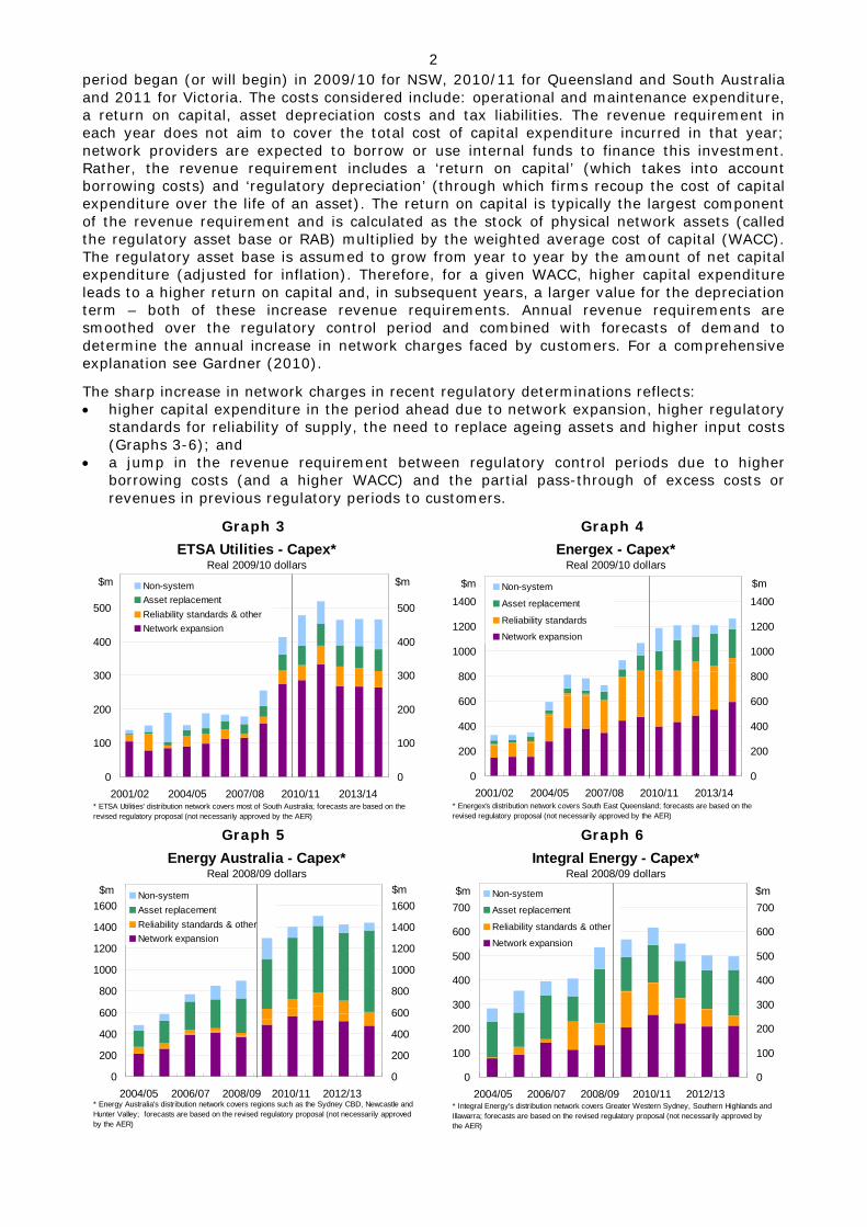
The sharp increase in network charges in recent regulatory determinations reflects: • higher capital expenditure in the period ahead due to network expansion, higher regulatory

standards for reliability of supply, the need to replace ageing assets and higher input costs (Graphs 3-6); and

• a jump in the revenue requirement between regulatory control periods due to higher borrowing costs (and a higher WACC) and the partial pass-through of excess costs or revenues in previous regulatory periods to customers.

Graph 3

ETSA Utilities - Capex*Real 2009/10 dollars

0

100

200

300

400

500

2001/02 2004/05 2007/08 2010/11 2013/14 0

100

200

300

400

500

Non-systemAsset replacementReliability standards & otherNetwork expansion

$m $m

* ETSA Utilities' distribution network covers most of South Australia; forecasts are based on the revised regulatory proposal (not necessarily approved by the AER)

Graph 4

Energex - Capex*Real 2009/10 dollars

0

200

400

600

800

1000

1200

1400

2001/02 2004/05 2007/08 2010/11 2013/140

200

400

600

800

1000

1200

1400Non-system

Asset replacement

Reliability standards

Network expansion

$m $m

* Energex's distribution network covers South East Queensland; forecasts are based on the revised regulatory proposal (not necessarily approved by the AER)

Graph 5

Energy Australia - Capex*Real 2008/09 dollars

0

200

400

600

800

1000

1200

1400

1600

2004/05 2006/07 2008/09 2010/11 2012/13 0

200

400

600

800

1000

1200

1400

1600Non-systemAsset replacementReliability standards & otherNetwork expansion

$m $m

* Energy Australia's distribution network covers regions such as the Sydney CBD, Newcastle and Hunter Valley; forecasts are based on the revised regulatory proposal (not necessarily approved by the AER)

Graph 6

Integral Energy - Capex*Real 2008/09 dollars

0

100

200

300

400

500

600

700

2004/05 2006/07 2008/09 2010/11 2012/13 0

100

200

300

400

500

600

700Non-system

Asset replacement

Reliability standards & other

Network expansion

$m $m

* Integral Energy's distribution network covers Greater Western Sydney, Southern Highlands and Illawarra; forecasts are based on the revised regulatory proposal (not necessarily approved by the AER)

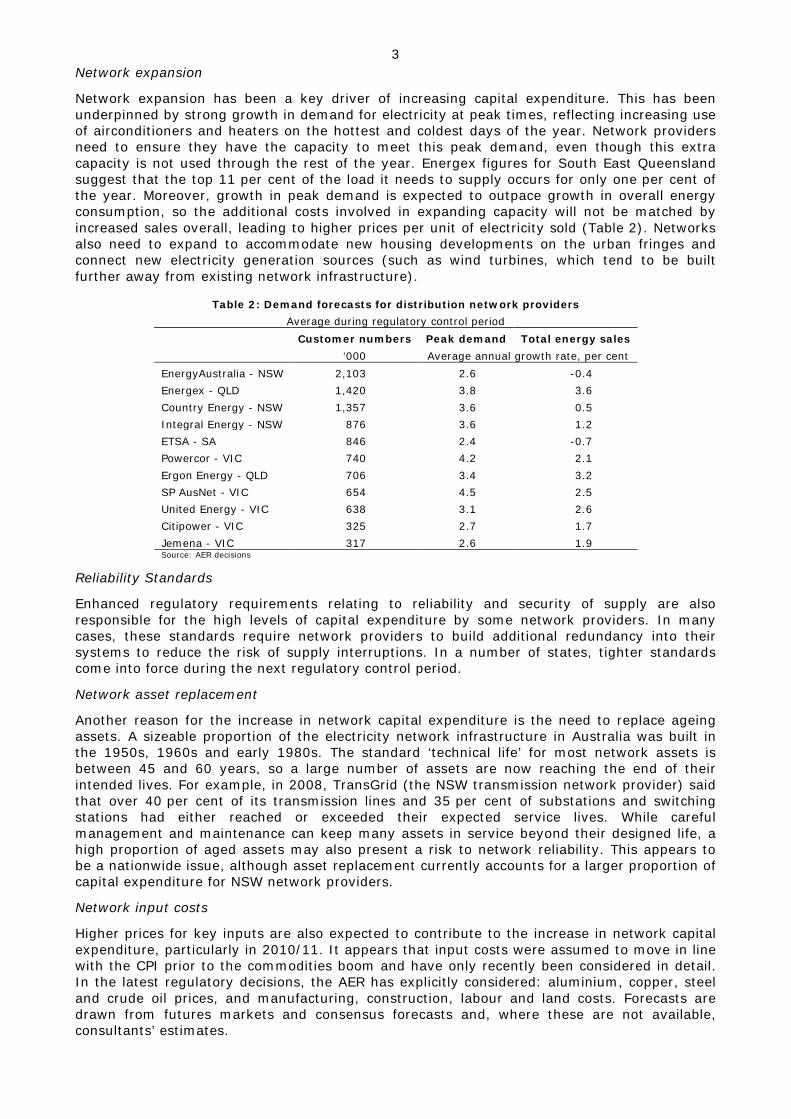
3 Network expansion

Network expansion has been a key driver of increasing capital expenditure. This has been underpinned by strong growth in demand for electricity at peak times, reflecting increasing use of airconditioners and heaters on the hottest and coldest days of the year. Network providers need to ensure they have the capacity to meet this peak demand, even though this extra capacity is not used through the rest of the year. Energex figures for South East Queensland suggest that the top 11 per cent of the load it needs to supply occurs for only one per cent of the year. Moreover, growth in peak demand is expected to outpace growth in overall energy consumption, so the additional costs involved in expanding capacity will not be matched by increased sales overall, leading to higher prices per unit of electricity sold (Table 2). Networks also need to expand to accommodate new housing developments on the urban fringes and connect new electricity generation sources (such as wind turbines, which tend to be built further away from existing network infrastructure).

Table 2: Demand forecasts for distribution network providers

Average during regulatory control period

Customer numbers Peak demand Total energy sales

‘000 Average annual growth rate, per cent

EnergyAustralia - NSW 2,103 2.6 -0.4

Energex - QLD 1,420 3.8 3.6

Country Energy - NSW 1,357 3.6 0.5

Integral Energy - NSW 876 3.6 1.2

ETSA - SA 846 2.4 -0.7

Powercor - VIC 740 4.2 2.1

Ergon Energy - QLD 706 3.4 3.2

SP AusNet - VIC 654 4.5 2.5

United Energy - VIC 638 3.1 2.6

Citipower - VIC 325 2.7 1.7

Jemena - VIC 317 2.6 1.9 Source: AER decisions

Reliability Standards

Enhanced regulatory requirements relating to reliability and security of supply are also responsible for the high levels of capital expenditure by some network providers. In many cases, these standards require network providers to build additional redundancy into their systems to reduce the risk of supply interruptions. In a number of states, tighter standards come into force during the next regulatory control period.

Network asset replacement

Another reason for the increase in network capital expenditure is the need to replace ageing assets. A sizeable proportion of the electricity network infrastructure in Australia was built in the 1950s, 1960s and early 1980s. The standard ‘technical life’ for most network assets is between 45 and 60 years, so a large number of assets are now reaching the end of their intended lives. For example, in 2008, TransGrid (the NSW transmission network provider) said that over 40 per cent of its transmission lines and 35 per cent of substations and switching stations had either reached or exceeded their expected service lives. While careful management and maintenance can keep many assets in service beyond their designed life, a high proportion of aged assets may also present a risk to network reliability. This appears to be a nationwide issue, although asset replacement currently accounts for a larger proportion of capital expenditure for NSW network providers.

Network input costs

Higher prices for key inputs are also expected to contribute to the increase in network capital expenditure, particularly in 2010/11. It appears that input costs were assumed to move in line with the CPI prior to the commodities boom and have only recently been considered in detail. In the latest regulatory decisions, the AER has explicitly considered: aluminium, copper, steel and crude oil prices, and manufacturing, construction, labour and land costs. Forecasts are drawn from futures markets and consensus forecasts and, where these are not available, consultants’ estimates.

4 Input cost assumptions vary somewhat across states depending on the timing of their regulatory reviews (Table 3). Decisions for Queensland and South Australia in May 2010 assumed that prices for key commodity inputs will rise by between 20 and 35 per cent in 2010/11, while the NSW decision in April 2009 assumed much smaller price increases.

Table 3: Key Commodity Price Assumptions

Real, per cent

Queensland and

South Australia(a) NSW(b)

2009/10 2010/11 2009/10 2010/11

Aluminium -7.0 23.0 -14.1 9.1

Copper 17.4 20.0 -10.8 2.1

Steel -28.3 33.0 -15.3 7.2

Crude Oil -3.7 25.8 -5.2 10.2 (a) Decisions made in May 2010 (b) Decision made in April 2009 Source: AER decisions

While the AER does not publish the expected aggregate increase in network input costs, our calculations (based on the limited information available) suggest that real input costs for Queensland network provider Energex will rise by around 7½ per cent in 2010/11 (see Appendix 1 for details). This suggests that input costs are a key driver of the increase in Energex’s capital expenditure in 2010/11, which is estimated to be roughly around 10 per cent (in real terms). However, large increases in capital expenditure are not always associated with rising input costs; input costs for Energex are estimated to have fallen by around 3 per cent in 2008/09 and 2009/10, while capital expenditure rose sharply.

Higher borrowing costs

Higher borrowing costs following the financial crisis are largely responsible for the increase in the WACC in recent regulatory decisions. The WACC rose by 126 basis points between regulatory decisions for the Queensland distribution networks, 80 basis points for South Australia and approximately 120 basis points for NSW.3

The increase was driven by higher debt raising costs (over and above the risk-free rate, CGS yields). As an aside, volatility in CGS yields led to considerable changes in the WACC for NSW network providers during the regulatory decision-making process; the WACC fell from 9.72 per cent at the time of the draft decision to 8.80 per cent in the final decision. The network providers took the AER’s final decision to the Australian Competition Tribunal, which decided that the averaging period used by the AER was unrepresentative and the WACC was raised to 10.02 per cent.

Given the size of the asset bases involved (the largest Queensland and NSW distribution networks had asset bases of around $7-8 billion each at the start of the regulatory period), even small changes in the WACC can make a large difference to the calculated return on assets and, therefore, total revenue requirements and prices. The effect appears to have been most pronounced in the Brisbane electricity market (where the increase in the WACC was largest). Our estimates suggest that of the 10 per cent real increase in Brisbane electricity prices in 2010/11, roughly around 4 percentage points was due to the assumed increase in the WACC (more details will be provided in Davis (2010), forthcoming).

Pass-through

In making a new regulatory decision, the AER considers each network provider’s actual revenues and capital expenditure relative to the forecasts contained in previous decisions. If actual capital expenditure or costs exceed what was forecast, networks are allowed to recoup some of these costs next period.4

On the other hand, if network providers earn more revenue than was allowed in the previous regulatory decision (due to underinvestment, efficiency gains or higher sales), some of this excess revenue will be passed back to customers in the form of lower prices in the next regulatory period.

3 The WACC for NSW was calculated on a different basis in the previous regulatory period, so this estimate is only indicative. 4 The AER allows the costs associated with certain unforseen events to be passed through to customers during the regulatory control period. These ‘events’ include: regulatory changes, changes in service standards, tax changes and, in some cases, events where insurance does not adequately cover losses.

5 Under- or over-expenditure on network infrastructure affects the next period’s revenue requirement through adjustments to the regulatory asset base. If actual capital expenditure exceeded what was forecast, the RAB would turn out to be higher at the start of the new regulatory control period than the closing RAB at the end of the previous regulatory period. This would lead to a step up in the return on capital and regulatory depreciation – and, therefore, the revenue requirement – in the first year of the new regulatory period.

For network providers in Queensland, actual capital expenditure in the 2005/06-2009/10 regulatory period was significantly above the forecast in the regulatory determination. This additional capital expenditure was responsible for between 15 per cent and around a third of the increase in their revenue requirements for 2010/11.

In contrast, Victorian distribution network providers are currently earning revenues that are higher than what was allowed in the regulatory determination (due to lower expenditure and higher sales). The AER’s draft decision for the 2011-2015 period proposes to pass some of this excess revenue back to customers through lower prices. This contrasts with the networks’ submissions suggesting that they need higher network charges to cover the costs associated with future increases in capital expenditure. The AER notes that the Victorian networks forecast very large increases in capital expenditure in previous regulatory periods; these expenditure forecasts were reduced to some extent by the regulator; yet the networks’ actual expenditure had been consistently lower than what the regulator had allowed. Further, this did not appear to be due to under-investment in infrastructure, as Victorian network providers have relatively high service standards compared to other states. Nevertheless, it is not yet clear if this decision will flow through to the prices Victorians actually pay for electricity, as significant revisions can occur between draft and final decisions, and increases in the other (unregulated) components of retail electricity prices could offset any falls in network charges.

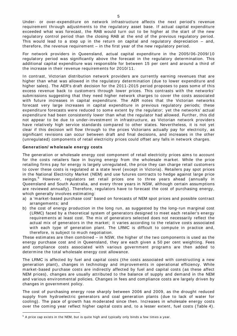
Generation/wholesale energy costs

The generation or wholesale energy cost component of retail electricity prices aims to account for the costs retailers face in buying energy from the wholesale market. While the price retailing firms pay for energy is largely unregulated, the price they can charge retail customers to cover these costs is regulated at a state level (except in Victoria). Retailers pay spot prices in the National Electricity Market (NEM) and use futures contracts to hedge against large price swings.5

a) a ‘market-based purchase cost’ based on forecasts of NEM spot prices and possible contract arrangements; and

However, regulators set retail prices one to three years ahead (annually in Queensland and South Australia, and every three years in NSW, although certain assumptions are reviewed annually). Therefore, regulators have to forecast the cost of purchasing energy, which generally involves estimating:

b) the cost of energy production in the long run, as suggested by the long-run marginal cost (LRMC) faced by a theoretical system of generators designed to meet each retailer’s energy requirements at least cost. The mix of generators selected does not necessarily reflect the actual mix of generators in the market; it varies according to the relative costs associated with each type of generation plant. The LRMC is difficult to compute in practice and, therefore, is subject to much negotiation.

These estimates are then combined – in NSW, the higher of the two components is used as the energy purchase cost and in Queensland, they are each given a 50 per cent weighting. Fees and compliance costs associated with various government programs are then added to determine the total wholesale energy cost allowance.

The LRMC is affected by fuel and capital costs (the costs associated with constructing a new generation plant), changes in technology and improvements in operational efficiency. While market-based purchase costs are indirectly affected by fuel and capital costs (as these affect NEM prices), changes are usually attributed to the balance of supply and demand in the NEM and various environmental policies. Changes in fees and compliance costs are largely driven by changes in government policy.

The cost of purchasing energy rose sharply between 2006 and 2009, as the drought reduced supply from hydroelectric generators and coal generation plants (due to lack of water for cooling). The pace of growth has moderated since then. Increases in wholesale energy costs over the coming year reflect higher capital costs and, to a lesser extent, fuel costs (Table 4).

5 A price cap exists in the NEM, but is quite high and typically only binds a few times a year.

6 In NSW, these higher energy costs were expected to be partly offset by an easing in the compliance costs associated with the state’s Greenhouse Gas Abatement Scheme.

Table 4: Wholesale Energy Cost Components

$/mwh, nominal

Energy Australia Integral Energy Country Energy Queensland

retailers

2009/10 2010/11 2009/10 2010/11 2009/10 2010/11 2009/10 2010/11

LRMC 55.3 67.9 57.3 70.0 46.9 63.2 53.6 58.6

Market-based purchase costs 63.7 45.3 67.0 47.0 56.6 43.3 54.8 58.5

Cost of energy 63.7 67.9 67.0 70.0 56.6 63.2 54.2 58.6

% increase 6.6 4.5 11.6 8.0

Fees & compliance costs 11.6 8.4 13.6 9.7 14.9 11.3 5.7 6.6

Wholesale energy costs 75.3 76.3 80.6 79.8 71.5 74.4 59.9 65.2

% increase 1.3 -1.0 4.1 8.7

Sources: IPART; QCA

Generation fuel costs

The fuel costs that affect electricity generators are primarily coal and natural gas prices.6

Fuel costs are assumed to have increased since the last regulatory determination, largely due to higher natural gas prices, while coal prices are expected to rise only modestly in real terms (if at all, depending on the timing of the decision for each state).

The price electricity generators pay for coal is significantly below world coal prices and, in aggregate, is not expected to increase in line with the rise in coal export prices. In Victoria, South Australia and some power stations in Queensland, the coal supply is owned by the power station, and the cost of coal is simply the cost of mining and transporting coal to the power plant. Generators that buy coal from third parties (in NSW and Queensland) also pay prices that are significantly below coal export prices. As at early 2009, most coal in NSW was still being supplied under contracts written before the surge in world coal prices from early 2004. As these contracts expire, new coal contracts will be set in an environment of higher export prices. However, regulators assume that generators will be able to get a discount of around 20 per cent to coal export prices as they: offer to take non-exportable coal; enter into very long term contracts; offer firm contracts to new developments; and often gain access to underdeveloped resources and employ a contract miner to produce the coal.

In the situations where higher export prices will lead to higher fuel costs for generators, the assumptions used in recent regulatory decisions appear to have underestimated the rebound in coal export prices that is now expected through 2010. However, regulators have committed to review the fuel costs assumptions used in their pricing decisions on an annual basis, which could result in upward revisions in future years.

Regulatory decisions assume gas prices have increased sharply over the past year and expect prices to rise a little further in real terms. This appears to reflect a change in the focus of many Australian gas providers away from domestic supply towards developing LNG export capacity.

Generation capital costs

The capital costs associated with building a new plant (including planning and approval, engineering, construction, land acquisition and infrastructure costs), used in the LRMC calculation, have increased sharply in recent years. This reflects higher prices for commodity inputs such as steel and higher labour costs. For example, in the latest NSW determination, capital costs were assumed to have risen by around 30-40 per cent, depending on the kind of generation plant (Graph 9). As with fuel costs, capital costs are reviewed on an annual basis and may be revised along with changes in commodity price forecasts in future determinations.

Other factors affecting the market-based purchase cost

Estimates of market-based purchase costs are based on detailed technical modelling, and discussion of the broader market developments underlying the forecasts is rather limited. NSW regulators attributed the high market-based purchase cost estimates in 2009/10 to uncertainty

6 In 2007/08, coal generation produced around 85 per cent of the NEM’s scheduled load.

7 about the effects of the drought, government environmental policies and ownership changes in the generation market. These price pressures are expected to ease somewhat in 2010/11.

There are notable differences in the market-based purchase cost allowance across states (even though electricity is purchased from the same ‘National’ Electricity Market). This partly reflects actual differences in the NEM spot prices faced by retailers in each state as network capacity constraints limit the amount of electricity transmitted across state borders (Graph 10). Purchase cost estimates can also vary by retailer depending on the timing and duration of peaks and troughs in demand from their customers relative to developments in the rest of the market. Estimates of market-based purchase costs also differ between states due to differences in their methodologies and assumptions, and the frequency with which assumptions are updated.

Graph 9

Assumed Capital Costs - NSWReal 2009/10 $/kW

0

500

1000

1500

2000

Coal Combined Cycle Gas Open Cycle Gas0

500

1000

1500

2000

2005-09 Decision2010-14 Decision

$ $

Sources: ACIL; Frontier Economics

Graph 10

Wholesale Electricity PricesLevel

0

25

50

75

100

125

150

2000 2002 2004 2006 2008 20100

25

50

75

100

125

150

$/MWh

VIC

SA

QLD

NSW

$/MWh

Source: NEMMCO / AEMO

Fees and compliance costs

Fees and compliance costs generally include the costs of complying with the Renewable Energy Target (RET), meeting obligations under state environmental schemes (such as the NSW Greenhouse Gas Abatement Scheme (GGAS) and the NSW Energy Efficiency Scheme (EES)) and NEM fees. It also includes compensation for energy losses that occur during transmission. Compliance costs were expected to fall in NSW in 2010/11 due to the phasing out of the GGAS scheme as the CPRS was to be introduced; while the CPRS has been delayed and the GGAS scheme has been extended, it does not appear that compliance costs for 2010/11 have been revised up.7

Assessment

In summary, while electricity price inflation is expected to peak later this year, it is set to continue at a rapid pace. Expected future price increases are largely driven by higher network charges in most states. Increasing network charges reflect network expansion, tighter reliability standards, the need to replace ageing assets, higher input costs, higher borrowing costs and the pass-through of costs associated with excess capital expenditure in previous years. In contrast, network charges may fall in Victoria next year. Generation or wholesale energy costs are expected to increase in most states in 2010/11 due to higher capital costs and, to a lesser extent, fuel costs. In NSW, this increase was partly offset by an expectation of lower environmental compliance costs.

The main risks to the current forecasts include: significant falls in Victorian electricity prices reflecting lower network charges; upward revisions to the commodity price forecasts underpinning wholesale energy cost calculations; and in NSW, higher compliance costs reflecting the extension of the state Greenhouse Gas Abatement Scheme.

Kate Davis / Prices, Wages and Labour Market Section / 12 August 2010

7 The CPRS was expected to have an impact on the LRMC and market-based purchase cost but did not impact the fees and compliance costs component. While the CPRS component of the LRMC and market-based purchase cost have been removed from regulatory price increases, compliance costs appear to be unchanged.

8 Appendix 1: Input Costs To calculate an indicative estimate of total input costs, we combined the price growth assumptions for individual input costs for Queensland distribution network Energex (taken from the AER’s final decision) with information about the weight of inputs included in materials costs (from an SKM consultancy report written for Energex) and weights for other inputs (from a Wilson Cook & Co report on Country Energy). We assumed that internal and contract labour had equal weights. The results are presented in the table below, showing the contribution of key inputs to the estimated total input cost increase expected in each year.

Indicative Input Costs for Network Capital Expenditure - Energex (a)

Average Weight(b) 2008/09 2009/10 2010/11 2011/12 2012/13 2013/14 2014/15

Per cent Contribution to real increase, per cent

Materials 67.0 -3.4 -3.6 7.2 -0.3 0.1 -0.8 -1.1

Of which:

Aluminium 10.2 -1.9 -0.7 2.5 -0.1 0.0 -0.3 -0.4

Copper 3.7 -1.2 0.6 0.6 -0.2 -0.1 -0.3 -0.4

Steel 10.9 0.8 -3.2 3.7 0.1 0.1 -0.2 -0.3

Oil and other energy(c) 6.4 -1.1 -0.2 1.7 -0.2 0.0 -0.1 -0.2 Land/easements 4.0 0.1 0.1 0.1 0.1 0.1 0.1 0.1

Labour 29.0 0.2 0.5 0.1 0.2 0.4 0.4 0.5

Total input costs 100.0 -3.1 -3.0 7.4 0.0 0.5 -0.3 -0.6

Memo: Capex(d) ~25 ~15 ~10 4.1 -1.2 -1.2 3.6 a) Input cost forecasts and materials component weights from Energex; combined with weights for land, labour and materials from Country Energy; assumed half

of labour is contract based and half is internal b) Average over period shown c) Energex uses oil prices to proxy for energy costs d) The increases in capital expenditure for 2008/09 to 2010/11 are uncertain as capital expenditure estimates that reflect the AERs adjustments to input costs are

not available Sources: AER decisions; SKM; Wilson Cook & Co

1

Developments in Utilities Prices

Utilities prices have been one of the fastest growing sub-groups of the consumer price index (CPI) in recent years, and further large increases are anticipated over the next few years. This follows subdued outcomes through most of the 1990s. Reasons behind the recent increases include the move towards cost-based pricing, the need to significantly increase investment to replace and expand infrastructure, and rising input costs. The effect of utilities price increases on CPI inflation has been significant – taking into account both direct and second-round effects, we estimate that utilities prices contributed around ½ percentage point to headline inflation and around 1/3 percentage point to underlying inflation over the past year. While inflation in Australian household electricity and gas prices since the 1990s has been towards the upper end of the range recorded in advanced economies – particularly over the past couple of years – the level of prices in Australia is around average.

Developments in Utilities Prices

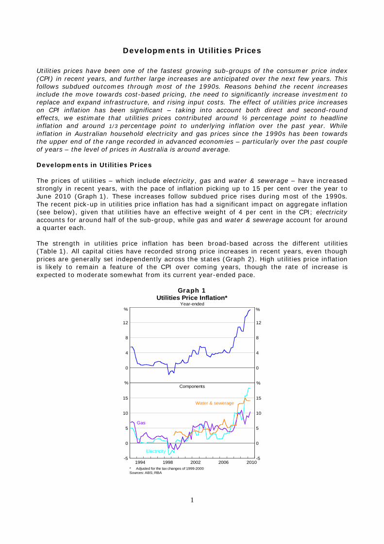
The prices of utilities – which include electricity, gas and water & sewerage – have increased strongly in recent years, with the pace of inflation picking up to 15 per cent over the year to June 2010 (Graph 1). These increases follow subdued price rises during most of the 1990s. The recent pick-up in utilities price inflation has had a significant impact on aggregate inflation (see below), given that utilities have an effective weight of 4 per cent in the CPI; electricity accounts for around half of the sub-group, while gas and water & sewerage account for around a quarter each.

The strength in utilities price inflation has been broad-based across the different utilities (Table 1). All capital cities have recorded strong price increases in recent years, even though prices are generally set independently across the states (Graph 2). High utilities price inflation is likely to remain a feature of the CPI over coming years, though the rate of increase is expected to moderate somewhat from its current year-ended pace.

Graph 1

0

4

8

12

0

4

8

12

-5

0

5

10

15

-5

0

5

10

15

Utilities Price Inflation*Year-ended

* Adjusted for the tax changes of 1999-2000Sources: ABS; RBA

2010

Electricity

%

2006200219981994

%

%%Components

Water & sewerage

Gas

2

Table 1 Graph 2

Utilities in the Consumer Price Index June quarter 2010 By capital city; March 2001 = 100

Utilities Price Indexes

Sources: ABS; RBA2010

Index

85

100

115

130

145

160

175

85

100

115

130

145

160

175

Index

2008

Perth

Melbourne

200620042002

Sydney

AdelaideBrisbane

Effective weight

Inflation over the:

Year Previous five years (annualised)

Utilities 4.0 15.3 5.9

of which:

Electricity 2.1 18.2 5.5

Gas* 0.8 10.3 5.9

Water & Sewerage 1.0 14.0 6.7

* Includes other household fuels Sources: ABS; RBA

Market Structure and Pricing

Electricity1

The prices paid by households for utilities services are highly regulated, with different regulatory arrangements applying at the various stages of production. Electricity and gas prices are generally made up of three components:

and gas

• The wholesale component, which is the cost of buying energy. The wholesale price paid by retailing firms is largely unregulated, with wholesale electricity prices set in the National Electricity Market (NEM) and wholesale gas prices set in confidential contracts between retail firms and wholesalers.2

• The network component, which is the cost of distributing the service to the end-customer. This component is regulated by the Australian Energy Regulator (AER) for both gas and electricity networks, with prices reset every five years (in special circumstances, certain unforseen costs can be passed through to customers during the regulatory period).

However, a number of states regulate the amount that retailing firms can charge retail customers to cover these wholesale costs (prices are reset every one to three years, with annual reviews of certain parameters, depending on the state).

3

• The retail component, which includes retail operation costs, such as meter reading, billing, marketing, etc. In the case of electricity, this component is regulated in each state (except Victoria), with prices reset every one to three years. In the case of gas, this component is only regulated in NSW, South Australia and Western Australia.

As well as recovering these costs, retailers are allowed to make a ‘reasonable margin’. For example, allowable electricity retailer margins currently range from 3 to 6 per cent across the states.

1 For a more detailed discussion of how electricity prices are set, see Gardner (2010). 2 A price cap exists in the NEM, but it is quite high and typically only binds a few times a year. Note that Western

Australia is not part of the NEM. A spot market for gas exists in Victoria to allow market participants to trade imbalances between contracted gas supply quantities and actual requirements. An interstate short-term trading market for gas is expected to begin operating in September 2010.

3 Prices in Western Australia are regulated at the state level, rather than by the AER.

3

The relative importance of the components varies across the different utilities and by state. For example, in electricity, a typical breakdown of the final price would be 45 per cent for each of the wholesale and network components, and 10 per cent for the retail component. For gas, a typical breakdown would be around one-third for the wholesale component and one-half for the network component, with the retail component comprising the remainder.

Choice of provider, or ‘Full Retail Contestability’, has become a feature of both the electricity and gas markets in recent years, although a number of major providers are state owned.

Water & sewerage

Most water & sewerage services are still operated by state monopolies. Prices charged to households take into account several factors (not dissimilar to those for electricity and gas), including funding requirements for infrastructure replacement and building of new infrastructure (including desalination and recycling plants), bulk water costs and general operating costs.

Why are Utilities Prices Rising so Rapidly?

There are a number of factors behind the large increases in utilities prices over recent years.4

• Price setting has become increasingly based on costs. This has involved a more detailed analysis of costs in regulatory pricing decisions and giving regulatory bodies a greater mandate to pursue cost-based price increases, rather than social or political objectives. One consequence has been the unwinding of cross-subsidies between household and business customers, which has resulted in higher prices for households in some states.

While the specific factors vary across each of the utilities and from state to state, there are a number of common themes. Some of these relate to ‘catch up’ for the below-average price increases and under-investment during much of the 1990s – in real terms, utilities prices fell by 7 per cent between 1990 and 2000 – while others relate to changes in the structure of the market, input costs and funding costs. The common themes include:

5

• Price increases have resulted from the need to significantly increase investment, both to replace ageing infrastructure and to expand existing infrastructure. For water, the expansion includes building recycling and desalination plants. For electricity, this expansion has been partly required to accommodate the increasing ‘peakiness’ of energy demand, and to meet more stringent reliability standards. Under the pricing model used by the electricity network regulator, an increase in investment contributes to higher prices in the regulatory period, as network prices are set to cover an ‘annual revenue requirement’, which consists of ‘regulatory depreciation’ (through which firms recoup the cost of capital expenditure over the life of an asset), as well as a ‘return on capital’, operating expenditures and tax liabilities. Recently an increase in the assumed return on capital, which takes into account borrowing costs, has also contributed to utilities price increases (see Box).

• Rising input costs for generation fuels, including gas and coal. However, generators typically pay significantly less than the market price for these inputs, due to the use of long-term contracts, the use of non-exportable coal (which is lower-grade, and therefore cheaper) in the generation process, and vertical integration, whereby generators in some states own the mines where their coal is sourced. In the case of electricity, generation

4 For a more detailed discussion of recent drivers of electricity price increases, see Davis (2010). 5 To some extent, this unwinding began in the 1990s, with larger real falls in electricity prices for businesses than for

households.

4

costs also increased as the drought reduced supply from hydroelectric generators and coal generation plants (due to a lack of water for cooling). In addition, higher prices for inputs such as steel have increased the costs associated with infrastructure replacement and expansion.

Box: The Effect of Increases in the Cost of Capital on Electricity Prices

Large-scale network infrastructure expenditures have been common in the electricity industry in recent years, and are expected to continue. In determining network price increases for the five-year regulatory period, regulators allow for a commercial return on network assets. This is known as the weighted-average cost of capital (WACC), and is essentially a weighted-average of the return on equity and cost of debt.

The most recent price determinations were made between 2008 and 2010 – during and following the financial crisis – when the cost of debt was elevated compared to previous regulatory decisions made in the mid 2000s. Hence, assumed increases in the WACC led to higher network costs and ultimately contributed to significant increases in final prices. This effect appears to have been most pronounced in the Brisbane electricity market, where the WACC increased from 8.46 per cent to 9.72 per cent (between decisions made in April 2005 and May 2010). Of the 10 per cent increase in real electricity prices in Brisbane in 2010/11, we estimate that around 4 percentage points was due to the assumed increase in the WACC.

Network costs are determined for five-year periods, so any moderation in the cost of debt since the recent regulatory decisions will not be reflected in the WACC until the next round of regulatory decisions.

The Impact on Inflation

Direct effect

With an effective weight of 4 per cent in the CPI, large changes in utilities prices can have a significant effect on aggregate inflation. As an example, over the year to June 2010, utilities prices boosted CPI inflation by nearly ½ percentage point, relative to a counterfactual where they had grown in line with the rest of the CPI. Our forecasts, based on information from regulators and liaison, suggest that utilities prices could boost CPI inflation by an average of 0.2 percentage points per year over 2010 to 2012.

Given that regulatory pricing decisions should reflect long-run factors, another counterfactual is how CPI inflation would have evolved over the inflation-targeting period had the increase in utilities prices been distributed uniformly over this period, rather than concentrated in recent years.6

Prior to 2000, year-ended CPI inflation would have been around 0.1 percentage points higher on average, had utilities price inflation been evenly distributed since 1993. The maximum effect would have been over the year to March 1996, when CPI inflation would have been nearly 0.4 percentage points higher (Graph 3).

Since 1993, the average annual increase in utilities prices has been almost 4 per cent – higher than that observed in the 1990s, and lower than that seen in the 2000s – and this outcome would have generated a significantly different profile for aggregate inflation.

Post 2000, year-ended CPI inflation would have been around 0.1 percentage points lower on average, had utilities price inflation been evenly distributed through time, with the effects most pronounced in recent years. The maximum effect would have been over the past year, when CPI inflation would have been more than 0.4 percentage points lower than the actual outcome.

6 To avoid a series break in this counterfactual exercise, ‘utilities’ includes ‘property rates & charges’, which were grouped with ‘water & sewerage’ prior to September 1998. Series are adjusted for the tax changes of 1999-2000.

5

The effects on underlying inflation of distributing utilities price inflation evenly through time are smaller, but still significant; on average over the past five years, year-ended trimmed mean inflation would have been a little over 0.1 percentage points lower, with a maximum effect of 0.25 percentage points in the year to June 2010 (Graph 4).7

Graph 3

Graph 4

-0.50

-0.25

0.00

0.25

-0.50

-0.25

0.00

0.25

-0.50

-0.25

0.00

0.25

-0.50

-0.25

0.00

0.25

Effect on CPI InflationEffect of smoothing utilities inflation*; year-ended

* Assumes utilities price inflation of 4 per cent per annum from 1993.Includes property rates & charges.

Sources: ABS; RBA

2010

ppts

2006200219981994

ppts

-0.50

-0.25

0.00

0.25

-0.50

-0.25

0.00

0.25

Effect on Trimmed Mean InflationEffect of smoothing utilities inflation*; year-ended

* Assumes utilities price inflation of 4 per cent per annum from 1993.Includes property rates & charges.

Sources: ABS; RBA

2010

ppts

2006200219981994

ppts

Indirect effect

There is also some evidence of second-round effects of utilities prices on inflation, whereby the impact of high utilities price inflation on input costs subsequently leads to higher inflation in other goods and services. Our analysis suggests that a 10 percentage point increase in utilities price inflation is associated with a 0.3–0.4 percentage point increase in underlying inflation, over and above the direct effects, with a lag of around two quarters. This implies that the above-average utilities price increases over the past few years could have contributed around 0.1 percentage points per year (on average) to inflation, via the effect on the prices of other goods, in addition to the direct effects outlined above. In contrast, below-average utilities price increases during parts of the 1990s would have had the opposite effect (albeit smaller).

The estimates of second-round effects were derived in two ways – both of which try to identify the effect of utilities price increases on inflation, over and above the direct effects – and provided very similar results:

• The first approach regressed underlying inflation ex-utilities on a range of usual variables (e.g. import prices, labour market variables and inflation expectations), but included utilities price inflation as an independent variable. Across a number of specifications, the coefficient on the utilities inflation variable was significant, with an elasticity of 0.03-0.04 and the peak effect occurring with a lag of two quarters.

• The second approach looked at input-output tables, and the extent to which utilities are used as an input in the production of other goods and services. This analysis also suggested an (upper bound) elasticity of aggregate inflation to changes in utilities prices of around 0.03-0.04.

7 This assumes that the rest of the price distribution was unchanged.

6

A Comparison of Utilities Price Developments in Advanced Economies8

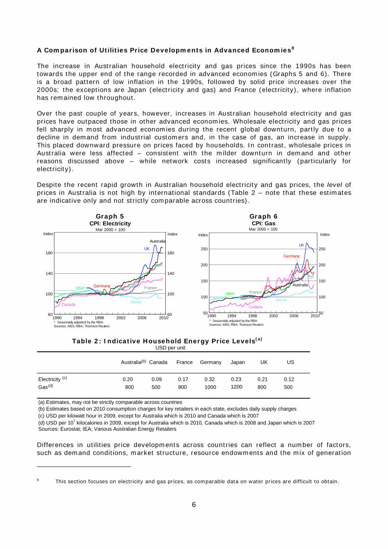
The increase in Australian household electricity and gas prices since the 1990s has been towards the upper end of the range recorded in advanced economies (Graphs 5 and 6). There is a broad pattern of low inflation in the 1990s, followed by solid price increases over the 2000s; the exceptions are Japan (electricity and gas) and France (electricity), where inflation has remained low throughout.

Over the past couple of years, however, increases in Australian household electricity and gas prices have outpaced those in other advanced economies. Wholesale electricity and gas prices fell sharply in most advanced economies during the recent global downturn, partly due to a decline in demand from industrial customers and, in the case of gas, an increase in supply. This placed downward pressure on prices faced by households. In contrast, wholesale prices in Australia were less affected – consistent with the milder downturn in demand and other reasons discussed above – while network costs increased significantly (particularly for electricity).

Despite the recent rapid growth in Australian household electricity and gas prices, the level of prices in Australia is not high by international standards (Table 2 – note that these estimates are indicative only and not strictly comparable across countries).

Graph 5 Graph 6

60

100

140

180

60

100

140

180

* Seasonally adjusted by the RBASources: ABS; RBA; Thomson Reuters

CPI: ElectricityIndex Index

JapanCanada

UK

USA* France

Mar 2000 = 100

201020062002199819941990

Australia

Germany

50

100

150

200

250

50

100

150

200

250

* Seasonally adjusted by the RBASources: ABS; RBA; Thomson Reuters

CPI: Gas

Index Index

Canada

USA*Japan

UK

France

Mar 2000 = 100

Germany

Australia

201020062002199819941990

Differences in utilities price developments across countries can reflect a number of factors, such as demand conditions, market structure, resource endowments and the mix of generation

8 This section focuses on electricity and gas prices, as comparable data on water prices are difficult to obtain.

Australia Canada France Germany Japan UK US

Electricity (c) 0.20

(b)

0.09 0.17 0.32 0.23 0.21 0.12 Gas (d) 800 500 900 1000 1200 800 500

(a) Estimates, may not be strictly comparable across countries

(c) USD per kilowatt hour in 2009, except for Australia which is 2010 and Canada which is 2007 (d) USD per 107 kilocalories in 2009, except for Australia which is 2010, Canada which is 2008 and Japan which is 2007

Table 2: Indicative Household Energy Price Levels(a) USD per unit

Sources: Eurostat; IEA; Various Australian Energy Retailers

(b) Estimates based on 2010 consumption charges for key retailers in each state, excludes daily supply charges

7

technologies. While a cross-country comparison of these factors is beyond the scope of this note, it is worthwhile noting the differences in electricity generation technologies across a range of advanced economies (Table 3). Australia is more heavily reliant on coal generation than many other advanced economies, while Canada generates around 60 per cent of its electricity from hydroelectric sources. According to CSIRO estimates (for Australia), the cost of coal generation is typically less than gas, wind, solar or nuclear power generation, but broadly in line with the cost of hydroelectric generation.

Michael Plumb, Kate Davis and Luke Brown Prices, Wages & Labour Market section Economic Group 8 October 2010

Australia Canada France Germany Japan UK US

Coal 85 19 6 51 30 36 49 Gas 8 4 4 12 28 42 22 Nuclear 14 87 23 25 16 19 Renewable (b) 7 61 2 12 3 4 9 Other 0 3 1 2 15 2 2

(a) Data are indicative; shares are for 2009 for Australia and 2007 for other countries (b) Includes hydroelectric generation Sources: EIA; IEA

Table 3: Electricity Generation by Fuel Type(a)

Per cent

How tight is Australia’s Rental Market?

This note discusses conditions in the Australian rental market. We find that conditions remain relatively tight across most of the capital cities, with some conjecture regarding conditions in the resource-rich states, although on most measures they appear to be noticeably weaker than in other state capitals. While conditions can be classified as broadly tight, the rental market has loosened somewhat over the past 18 months with rental growth slowing and vacancy rates rising moderately. Looking forward, we anticipate that conditions will tighten over the next few years, primarily due to the mining boom increasing rental demand in Perth and Brisbane.

The national vacancy rate fell to 1.9 per cent in the June quarter, although remains 0.5 percentage points above its trough in the June quarter 2008 (Graph 1). Trends in the vacancy rate have been broadly consistent with ABS real rental growth, which had slowed by around 2 percentage points since the December quarter 2008, but has recently ticked up. Overall, the vacancy rate remains below its decade average of 2.5 per cent and real rental growth is well above its decade average of 1.1 per cent.

Graph 1

Graph 2

Growth in newly negotiated rents, which tend to lag vacancy rates by around six months, has picked up a little over the past 12 months (Graph 2). Although rental growth was flat in the June quarter, rents rose by 6.3 per cent over the year to the June quarter, broadly consistent with the recent fall in the national vacancy rate. Cities with tighter rental conditions

While rental conditions are fairly tight nationally there is dispersion in the disaggregated capital city data. Presently rental market conditions in Sydney, Melbourne and Adelaide appear to be tight.

• Sydney: The vacancy rate was 1.2 per cent in the June quarter, which is just 0.3 percentage points above its trough in the December quarter 2007 (Graph 3; Table 1). Abstracting from the current episode, vacancy rates in Sydney are at their lowest level since the late 1980s. Despite this, year-ended growth in real rents has slowed from 5.7 per cent in the June quarter 2009, to 1.9 per cent by the June quarter 2010. The slowdown in rental growth is likely due in part to payback from very fast growth in 2009, and is unlikely to continue given current vacancy rates. This is supported by growth in newly negotiated rents, where growth peaked at almost 17 per cent in the June quarter 2008 before slowing in 2009 and rising again in recent quarters (Graph 4).

-4

-2

0

2

4

60

1

2

3

4

1984 1987 1990 1993 1996 1999 2002 2005 2008

Vacancy Rates and RentsAustralia

Real CPI rents (y-e; RHS; inverted)*

Vacancy Rate (sa) (LHS)

Sources: ABS; RBA; REIA

%%

* Calculated as the CPI measure of rents relative to underlying inflation-3

0

3

6

9

12

15

-3

0

3

6

9

12

15

1994 1997 2000 2003 2006 2009

Year-ended

Quarterly

% %

REIA Rental GrowthPercentage change

Sources: REIA; RBA

Graph 3

Graph 4

• Melbourne: Rental vacancy rates loosened a little over recent quarters but are still fairly tight by historical standards. The vacancy rate was 1.5 per cent in the June quarter, having increased by 0.5 percentage points since its trough in June quarter 2008. Despite this, the vacancy rate remains around 1.2 percentage points below its decade average. Similar to Sydney, real rental growth has fallen of late, after recording very strong growth in 2009. Newly negotiated rents increased by 8.9 per cent over the year to the June quarter, pointing to strong CPI rent growth going forward.

Table 1

• Adelaide: The vacancy rate remains at a very low level in Adelaide, at around 1.0 per cent in the June quarter, its lowest level since early 2007. Despite this, annual real rental growth has slowed from 3.8 per cent to 1.4 per cent over the past year. Rental growth in Adelaide has been noticeably weaker than in either Sydney or Melbourne, despite a comparable vacancy rate.

Cities with looser rental conditions

Rental market conditions in Brisbane and Perth appear noticeably looser at present. We anticipate, however, that rental conditions in both these cities will tighten over the next few years as new supply fails to keep pace with demand generated by the resource boom.

• Brisbane: Rental market conditions loosened noticeably in Brisbane over the past two years (Graph 5). The vacancy rate was at 3.8 per cent in the June quarter and almost 3 percentage points above its early 2007 trough. Annual real rental growth has slowed rapidly, from 6.0 per cent at the beginning of 2009 to just 0.5 per cent in

-6

-4

-2

0

2

4

6

8

10-2

-1

0

1

2

3

4

5

1984 1993 2002 1984 1993 2002

Vacancy Rates and Rents

* Deflated by state CPI.Sources: ABS; REIA; RBA

% Sydney Melbourne %

Real CPI rents y-e (RHS; inverted)*

Vacancy rate (LHS)

-10

-5

0

5

10

15

-10

-5

0

5

10

15

1997 2000 2003 2006 2009

Newly Negotiated Rental GrowthQuarterly percentage change

% %

Melbourne

Sydney

Sources: ABS; RBA; REIA

Rental Market Indicators*Vacancy Vacancy Vacancy Real Rental Real Rental Real Rental

Rate Rate Rate Growth (YE) Growth (YE) Growth (YE)June Qtr Decade Avg Trough / current June Qtr Decade Avg Peak / current

Sydney 1.2 2.5 0.3 1.9 0.6 -3.8Melbourne 1.5 2.7 0.5 1.0 0.1 -3.8Brisbane 3.8 2.6 2.9 0.5 1.4 -5.5Adelaide 1.0 2.0 0.4 1.4 0.5 -2.4Perth 3.6 3.1 2.6 0.1 1.4 -8.5Australia** 1.9 2.5 0.6 1.9 1.1 -2.1* Vacancy rate level and real rental grow th in percentages; trough/peak-to-current in percentage points.** State data deflated by headline state CPI; national by underlying CPI.Sources: ABS; RBA; REIA

the June quarter, which is broadly consistent with the rise in the vacancy rate. Growth in newly negotiated rents slowed significantly over 2009 and has remained subdued in recent quarters (Graph 6).

Graph 5

Graph 6

• Perth: Similar to Brisbane, rental conditions loosened considerably in Perth over 2009, but have since tightened somewhat. According to REIA, the rental vacancy rate climbed to 5.4 per cent in the March quarter before falling to 3.6 per cent in the June quarter. The sharp rise in vacancy rates has corresponded with a fall in rents, with real rental growth falling to 0.1 per cent over the year to the June quarter from 8½ per cent at its peak in March quarter 2009. The pace of growth in newly negotiated rents fell rapidly during 2009, but has picked-up modestly since.

Other vacancy measures – SQM

The REIA measures of rental vacancies just considered suggest that conditions in Brisbane and Perth loosened significantly over the past 18 months. However alternative measures suggest that conditions are actually somewhat tighter within the resource-rich states. SQM Research produce a monthly rental vacancy series based on online monitoring of major rental listing sites. SQM have suggested that their measure is superior due to a broader scope and other methodological differences, although there are concerns about SQM’s capacity to identify and remove duplicate vacancies.1

The SQM measure suggests that rental conditions in

Perth were significantly tighter than indicated by the REIA measure, trending down to 1.4 per cent in August (compared with 3.6 per cent according to REIA); although, consistent with REIA, this level is almost double the vacancy rate recorded by SQM during the 2005/06 episode. In Brisbane SQM are reporting a vacancy rate of 1.9 per cent (compared with 3.8 per cent for REIA); this is higher than the rate reported by SQM in 2006/07, and around the rate reported for 2005 and 2008. For the other capital cities, the SQM and REIA measures are broadly consistent.

Demand and Supply Factors

The rise in vacancy rates in Brisbane and Perth line up with trends in population. Population growth in the resource-rich states slowed to an annual rate of around 2¼ per cent in the March quarter 2010, from a peak of 3.4 per cent and 2.9 per cent for

1 SQM have suggested that REIA data may be less reliable due to the objectiveness of vacancy data from real

estate institutes. For more information, see: Media Watch. SQM data is collected on a weekly basis and the data is complemented with additional data from APM. One weakness of the SQM rental vacancy data is the length of the time series, which only goes back to the beginning of 2005, in comparison REIA data goes back to around 1980.

-9

-6

-3

0

3

6

9-2

0

2

4

6

8

1984 1993 2002 1984 1993 2002

Vacancy Rates and Rents

* Deflated by state CPI.Sources: ABS; REIA; RBA

% Brisbane Perth %

Real CPI rents y-e (RHS; inverted)*

Vacancy rate (LHS)*

-10

0

10

20

-10

0

10

20

1997 2000 2003 2006 2009

Newly Negotiated Rental GrowthQuarterly percentage change

% %

Perth

Brisbane

Sources: ABS; RBA; REIA

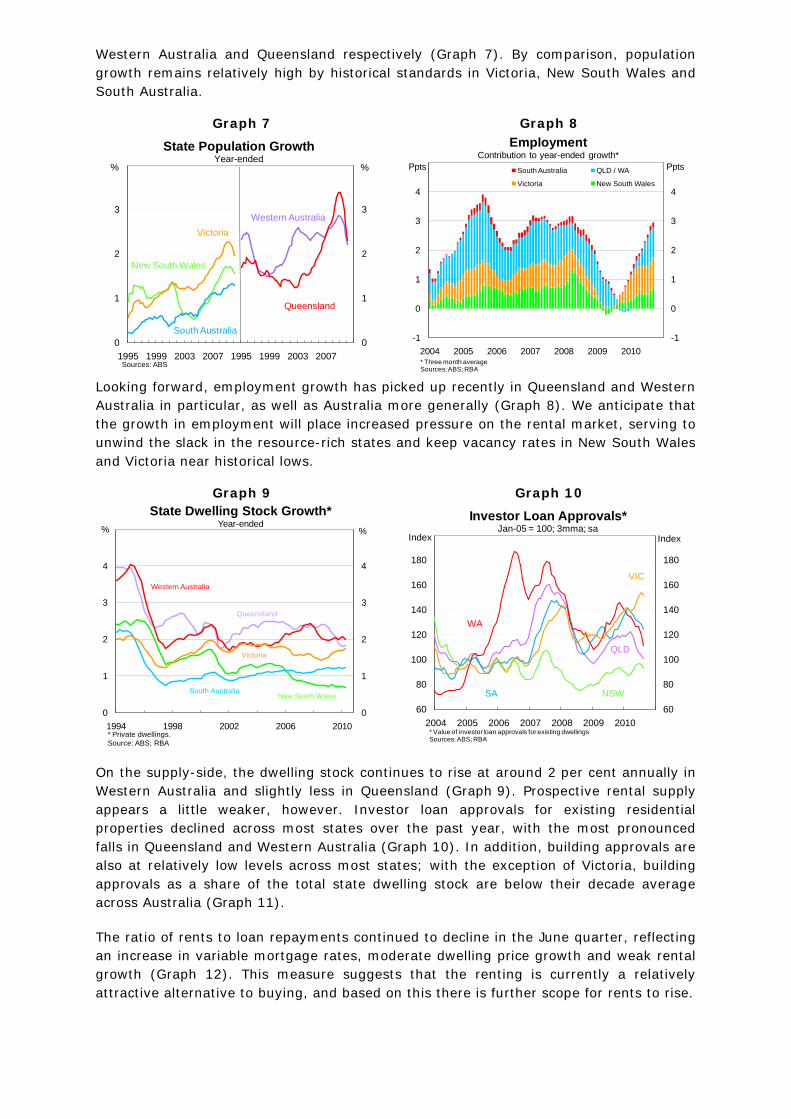
Western Australia and Queensland respectively (Graph 7). By comparison, population growth remains relatively high by historical standards in Victoria, New South Wales and South Australia.

Graph 7

Graph 8

Looking forward, employment growth has picked up recently in Queensland and Western Australia in particular, as well as Australia more generally (Graph 8). We anticipate that the growth in employment will place increased pressure on the rental market, serving to unwind the slack in the resource-rich states and keep vacancy rates in New South Wales and Victoria near historical lows.

Graph 9

Graph 10

On the supply-side, the dwelling stock continues to rise at around 2 per cent annually in Western Australia and slightly less in Queensland (Graph 9). Prospective rental supply appears a little weaker, however. Investor loan approvals for existing residential properties declined across most states over the past year, with the most pronounced falls in Queensland and Western Australia (Graph 10). In addition, building approvals are also at relatively low levels across most states; with the exception of Victoria, building approvals as a share of the total state dwelling stock are below their decade average across Australia (Graph 11).

The ratio of rents to loan repayments continued to decline in the June quarter, reflecting an increase in variable mortgage rates, moderate dwelling price growth and weak rental growth (Graph 12). This measure suggests that the renting is currently a relatively attractive alternative to buying, and based on this there is further scope for rents to rise.

0

1

2

3

0

1

2

3

1995 1999 2003 2007 1995 1999 2003 2007Sources: ABS

Western Australia

New South Wales

Victoria

Queensland

State Population GrowthYear-ended

% %

South Australia-1

0

1

2

3

4

-1

0

1

2

3

4

2004 2005 2006 2007 2008 2009 2010

EmploymentContribution to year-ended growth*

South Australia QLD / WA

Victoria New South Wales

* Three month averageSources: ABS; RBA

Ppts Ppts

0

1

2

3

4

0

1

2

3

4

1994 1998 2002 2006 2010

State Dwelling Stock Growth*Year-ended% %

Victoria

New South Wales

Queensland

South Australia

Western Australia

* Private dwellings.Source: ABS; RBA

60

80

100

120

140

160

180

60

80

100

120

140

160

180

2004 2005 2006 2007 2008 2009 2010* Value of investor loan approvals for existing dwellingsSources: ABS; RBA

QLD

NSW

VIC

SA

Investor Loan Approvals*Jan-05 = 100; 3mma; sa

Index Index

WA

Graph 11

Graph 12

These factors suggest that there is unlikely to be a large pick-up in the supply of rental properties over the next year, which coupled with still solid population and employment growth, and the current relative attractiveness of renting, suggests that there may be increasing pressure on rental markets in the year ahead. 2

Summary

Nationally, the rental market remains fairly tight despite loosening a little over the past two years. There are, however, some significant differences across the capital cities. The REIA measure of vacancy rates suggests that there is spare capacity in Perth and Brisbane, which is consistent with relatively weak rental and dwelling price growth throughout this period. By comparison, the SQM measure suggests that rental markets are tight across all capital cities.

With the resources boom expected to boost income growth and housing demand we anticipate that rental market conditions in Western Australia and Queensland will tighten significantly over the next few years. The supply side appears somewhat subdued across most states, with investor loan approvals falling and building approvals below their decade average. As a result, we expect national vacancy rates to trend downward through 2011, driven primarily by the resource-rich states, putting upward pressure on rents.

Callam Pickering Financial Conditions Section Economic Analysis Department 15 October 2010

2 See, Strickland (2010), Migrant Households and their Dwelling Characteristics, which suggests that recent

migrants have a higher propensity to rent.

0

1

2

3

0

1

2

3

1993 1997 2001 2005 2009

Private Dwellings ApprovedAs a proportion of total state dwelling stock; annualised

% %

Sources: ABS; RBA

Queensland / Western Australia

New South Wales

Victoria

30

40

50

60

70

80

90

100

10

15

20

25

30

35

40

45

1988 1992 1996 2000 2004 2008 1988 1992 1996 2000 2004 2008

Relative Dwelling Costs% %

Loan repayment

Rent payment

Rents to loan repayments, ratioPer cent of HHDY

Sources: RBA; APM; REIA

1

RECENT DEVELOPMENTS IN URBAN WATER PRICES

Water and sewerage prices have grown much faster than the CPI over recent years. This paper outlines how urban water prices are set in Australia, and discusses the drivers of recent and future urban water price increases. Broadly speaking, a significant pick-up in capital expenditure has been responsible for recent sharp prices increases and is expected to drive strong future increases in all mainland capital cities (except Sydney). A major reason behind the pick-up in capital expenditure has been to reduce the reliance of urban water suppliers on rainfall. This has been achieved mainly through the construction of desalination plants. To date three desalination plants have been commissioned, with another three plants (Melbourne, Adelaide and a second Perth plant) worth a total value of $6.3 billion expected to be completed by the end of 2012.

Background

Since mid 2008, water and sewerage prices have grown much faster than the consumer price index (Graph 1). This rise in water and sewerage prices has been broad-based, with all mainland capital cities experiencing strong price growth over this period (Graph 2). A key factor behind this has been the substantial growth in water and sewerage capital expenditure by water suppliers across the country (Graph 3).

Graph 1

Graph 2 Graph 3

Recent growth in water and sewerage capital expenditure has been aimed at reducing suppliers’ reliance on traditional rain-fed sources, which in 2008-09 accounted for around 85 per cent of Australia’s urban water supply (Table 1). The desire to diversify supply was driven by poor rainfall during the 2000s,1

1 Decade-average rainfall into agricultural areas was the lowest in a century during the 2000s. For further

information see

which saw water storage drop to very low levels, even though water usage per household declined due to successful demand-side management. For example, dam storage levels in Melbourne fell from

Trends in Farm Output and Exports.

0

4

8

12

0

4

8

12

Jun-1999 Jun-2002 Jun-2005 Jun-2008 Jun-2011* Adjusted for the tax changes of 1999-2000Source: ABS

Consumer Price Inflation*Year-ended

% %

Water and sewerage

All components

50

100

150

200

50

100

150

200

1998 2001 2004 2007 2010Source: ABS

Adelaide

Sydney

Melbourne

Perth

Water and Sewerage PricesIndex 1998-2002=100

Index IndexBrisbane

0.0

0.5

1.0

1.5

0.0

0.5

1.0

1.5

2003-04 2004-05 2005-06 2006-07 2007-08 2008-09* As reported by utilities servicing100 000+ propertiesSources: National Water Commission; RBA

Brisbane

Sydney

Melbourne

Perth

Water and Sewerage Capital Expenditure2008/09 prices*

$bn $bn

Adelaide

2

around 80-90 per cent of capacity during the 1990s to around 30-40 per cent during the 2000s. Dam storage levels would have fallen to below 15 per cent in Sydney in 2007 had diversions from the Shoalhaven River not been in place, while in Perth dam storage levels fell as low as 20 per cent in 2003.2

Since 2008-09, the sources of urban water supply have been gradually expanding. Desalination plants recently commissioned in NSW and Queensland have added capacity equivalent to 12 and 16 per cent of 2008-09 urban water supply in each of these states.3

Price setting

Price setting behaviour varies from state to state with prices set by an independent regulator (NSW, Victoria), the state government (Western Australia, South Australia) or council owned retailers (Queensland). Despite this, all states have established an independent body that is in some way involved in setting, reviewing or advising on price setting behaviour consistent with the principles set out by the National Water Initiative (NWI).4

In general, the first step in setting urban water prices is to determine an ‘annual revenue requirement’ for each of the years within the regulatory period (usually three to five years). This is determined using what regulators call a ‘building blocks’ approach, with the annual revenue requirement calculated as the sum of certain costs (or building blocks). Though some variation exists between states,

5

• Operating expenditures are the recurrent outlays required to provide water services, and include bulk water charges (where the bulk water provider and water retailer are not the same entity)

the building blocks are generally operating expenditure, a return on capital, and a return of capital (depreciation). This approach is similar to the ones used to determine electricity and gas network prices.

6

• The return on capital represents the opportunity cost of investment, and is calculated as the product of the regulated asset base (RAB) and the weighted

as well as the costs associated with maintenance and administration (e.g. billing and metering).

2 However, water from dams makes up a much smaller share of total urban water supply in Perth than in

other capital cities due to the use of groundwater. 3 The actual contribution from the Kurnell (Sydney) and Tugan (Gold Coast) desalination plants will vary from

year to year depending on usage. As desalination is a relatively expensive source of water, it will be used less when cheaper rain-fed sources are abundant. For example, following recent heavy rain, the Queensland government announced it would place the Tugan desalination plant on standby mode from the end of December 2010 to reduce water bills.

4 For further information about the NWI pricing principles, please see Appendix A. 5 According to the National Water Commission, a building blocks methodology is used in all major states

except Queensland. 6 This applies to retailers in Sydney, Melbourne, Perth and, more recently, South East Queensland. Bulk

water charges are determined using a building blocks methodology similar to that used for urban water prices.

Surface water1 Groundwater Desalination Recycled water Bulk water2 Total

New South Wales 91 3 0 2 4 100Victoria 87 4 0 4 5 100Queensland 35 1 0 5 59 100South Australia 83 2 0 15 0 100Western Australia 33 50 11 2 4 100Australia 74 10 1 4 11 1001 Includes rivers and dams

Source: National Water Commission

2 The total volume of water purchased from another utility or entity outside the urban utility's geographic area of responsibility (excluding urban bulk water suppliers)

Per centTable 1: Urban water supply sources 2008-09

3

average cost of capital (WACC). The RAB is a measure of the net value of existing capital and is recalculated each year to account for additions to the capital stock (net of disposals and depreciation). This method implicitly values the assets at their inflation-adjusted construction cost, less depreciation. For a number of retailers, recent increases in the return on capital have partly reflected a higher WACC, consistent with the increased cost of debt observed since the global financial crisis.

• Return of capital is the depreciation of the RAB. Through this term, water providers recoup the cost of capital expenditure over the life of an asset.

Once the annual revenue requirements have been determined, prices are set to recover these revenues over the regulatory period. Importantly, prices need not be set to recover the annual revenue requirement in each year of the regulatory period. Rather, prices can be smoothed over the regulatory period to limit the impact of sharp price increases on consumers. In setting prices, customer numbers as well as future demand need to be projected over the regulatory period.

Prices are generally structured as a two-part tariff. This involves a variable water usage charge and a fixed service availability charge. In principle, the usage charge should be set at the long-run marginal cost of supply.7 However, in practice, this does not occur as retailers tend to set multiple usage charges for equity reasons. Broadly speaking, the retailer will set a low water usage charge for an amount of water required to meet basic needs, with water used in excess of this amount billed at a higher rate.8

Recent annual revenue requirements

The fixed service availability charge is then calculated as the residual of the revenue requirement less total water usage charges.

Based on the latest regulatory reviews, operating costs account for 30 to 80 per cent of a retailer’s annual revenue requirement.9

This large variation between retailers reflects a number of factors. Firstly, as mentioned earlier, some retailers are more reliant on bulk water providers than others.

Similarly, the share of the annual revenue requirement made up of the return on capital varies considerably, from 10 to 50 per cent. The remainder, which is depreciation, typically accounts for a relatively small share of the annual revenue requirement.

10 These retailers will tend to have a greater proportion of their annual revenue requirement made up of operating expenses. Secondly, a number of retailers have recently undertaken substantial capital programs to construct additional water supply assets. For these retailers, the share of their annual revenue requirement attributable to capital expenditure is around 50 per cent.11

Despite this variation, increases in the annual revenue requirement of water retailers, up to 2008-09, have been largely driven by capital expenditures (Graph 4). An increase in capital expenditure immediately contributes to higher annual revenue requirements by raising the return on capital via a higher RAB. However, it will also contribute to higher revenue requirements in future years by increasing the return of capital (or depreciation). Considering the water industry as a whole, the recent growth in capital expenditure has been driven by increased spending on water assets, with expenditure on sewerage assets, such as treatment plants and pipes only increasing marginally (Graph 5).

7 This is consistent with the National Water Initiative Pricing Principles. 8 In 2008, IPART proposed to implement a one tier price for economic efficiency reasons. This would not

come into effect until after the current regulatory period, which ends in 2011/12. 9 This is based on water utilities servicing more than 100 000 properties. 10 This is due to different institutional arrangements. In some states, the bulk and retail water provider are

the same entity while in others they are completely separate. In addition, some retailers have their own sources of water such as desalination.

11 These retailers are SA Water and Water Corporation (Perth).

4

Graph 4 Graph 5

Future capital expenditure and prices

Looking ahead, according to the Water Services Association of Australia (WSAA) much of the expected growth in capital expenditure by the water industry will be to increase the security of water supply, though some spending on upgrading or constructing new wastewater infrastructure is also planned (Graph 6). Much of the capital expenditure on water assets will be for desalination plants. Of a total of around $11½ billion of major capital projects identified by the WSAA as under construction in 2010/11, $6.3 billion is expected to be spent on desalination plants

Graph 6

in Melbourne, Adelaide and Perth.12

A further $3 billion is expected to be spent on sewerage and maintenance, with the remainder spent on smaller water supply projects such as dams, recycling plants and connecting water supply assets.

Retail price changes are influenced by the size and timing of capital expenditure programs, whether an asset is owned by the bulk water supplier or retailer, and the change over between regulatory periods. These factors, particularly the timing and size of capital expenditure programs, will lead to a disparity in the strength of price growth observed between Sydney and the other major capital cities over the next couple of years. Growth in Sydney water prices is expected to be relatively moderate as the costs associated with constructing the Kurnell desalination plant have already been incorporated into the current level of water prices. In contrast, large future capital expenditure programs in other major capital cities have yet to be reflected in the retail price.

12 For further information on the location and capacity of desalination plants see Appendix Table A2.

0

1

2

3

0

1

2

3

2005-06 2006-07 2007-08 2008-09* For utilities servicing more than 100 000 propertiesSource: Water Services Association of Australia

Capital

Operating

Water Retailers' Expenditure*Annual, 2008-09 prices

$bn $bn

0

2

4

0

2

4

2005-06 2006-07 2007-08 2008-09* Includes expenditure by retail and bulk water providers Source: Water Services Association of Australia

Water

Sewerage

Urban Water Industry Capital Expenditure*Annual, major water utilities, 2008-09 prices

$bn $bn

0

2

4

0

2

4

Perth Melbourne Sydney SE Qld AdelaideSource: Water Services Association Australia; RBA

Supply

Other

Major Capital Projects Underway or to be commenced in 2010/11, nominal

$bn $bn

5

Summary

Water and sewerage prices have grown much faster than the CPI in recent years due to a substantial pick-up in capital expenditure by water retailers. Going forward, growth in water and sewerage prices is expected to remain strong as the water industry continues to spend significant amounts on increasing water security. A forthcoming note will address future directions in water pricing methodology, particularly focussing on whether water is currently underpriced. Nicholas Tan Regional and Industry Analysis Economic Group 4 February 2011

Sydney Melbourne* Adelaide* Perth* SE Qld*2008/09 16.8 13.2 8.1 4.0 11.22009/10 7.1 16.8 5.6 5.5 14.42010/11 4.9 15.4 8.9 5.7 8.52011/12 2.7 10.6 n/a 5.4 8.52012/13 n/a 7.6 n/a 5.1 n/a

Table 2: Real Water and Sewerage Prices

Sources: Various State Regulators; National Water Commission; RBA

* RBA estimate

Annual percentage increase

6

Appendix A: National Water Initiative and Pricing To help the states and territories meet the above commitments, NWI pricing principles were developed. These cover four broad areas: recovery of capital expenditure, setting urban water tariffs, recovering the costs of water planning and management and recycled water and stormwater reuse. For the NWI Pricing Principles please see web.

Table A1: Urban Water Supply and Price Regulation* Jurisdiction Urban water supplier Regulator

Sydney Sydney Water Corporation IPART

Melbourne City West Water

South East Water

Yarra Valley Water

Essential Services Commission

South East Queensland

Brisbane Water

Gold Coast Water

Local government councils reviewed by

Queensland Competition

Authority (QCA)

Adelaide SA Water

SA Cabinet and reviewed by Essential Services Commission

of South Australia (ESCOSA)

Perth Water Corporation Western Australia Cabinet with oversight by

Economic Regulation Authority (ERA)

* For utilities servicing 100 000 or more prroperties

7

City Location Capacity (ML/year)Share of 2008/09

residential supply1Upgradable to

(ML/year)Completion

Sydney Kurnell 90000 28 180000 CompletedMelbourne Wonthaggi 150000 67 200000 2011South East Queensland Tugan 49000 55 CompletedPerth Kwinana 45000 26 Completed

Binninyup 50000 29 100000 2011Adelaide Port Stanvac 100000 108 Dec-2012Total 484000 54 6740001 Only including utilities that service 100 000 or more properties

Table A2: Desalination Plants

Source: RBA; Water Services Association of Australia