Embed Size (px)
Citation preview

HowBigisYourNeighborhoodUsingtheAHSandGIS
to DeterminetheExtentofYourCommunityKwameDonaldsonPhDUSCensusBureau
June132013(updated)SEHSDWorkingPaperFY2013‐064
I am extremely grateful to Charles A Bee Aref N Dajani and Matthew B Streeter of the US Census Bureau and Michael K Hollar and David A Vandenbroucke of the US Department of Housing and Urban Development for their careful review of this report and their thoughtful feedback Since I did not make all of the changes suggested by them the reader should assume that any errors in this report reflect fixes that I neglected to make despite their recommendations
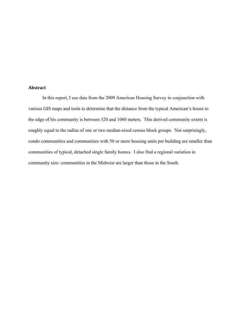
Abstract
In this report I use data from the 2009 American Housing Survey in conjunction with
various GIS maps and tools to determine that the distance from the typical Americanrsquos house to
the edge of his community is between 520 and 1060 meters This derived community extent is
roughly equal to the radius of one or two median-sized census block groups Not surprisingly
condo communities and communities with 50 or more housing units per building are smaller than
communities of typical detached single family homes I also find a regional variation in
community size communities in the Midwest are larger than those in the South
Table of Contents
Introduction 1
A Simple Method 4
The Kappa Coefficient 10
The Maximum Kappa Coefficient and the Derived Community Extent 14
Maximum Kappa Coefficients and Derived Community Extents for Various Demographic and
Socioeconomic Groups 20
An Alternative Method for Deriving Neighborhood Size 24
Conclusion 34
References 35
Appendix A The Neighborhood Quality Section of the 2009 AHS 37
Appendix B Selected Statistics and Tabulation Area Counts by State 40
Introduction
In a brief review of the academic literature on neighborhoods one researcher notes that
the term has not been well-defined (Taylor 2012) He reports that researchers have been trying
to build consensus around a definition of neighborhood or community for more than a century
yet these terms remain ldquosome of the most notoriously slippery social science conceptsrdquo Part of
the difficulty in settling on a suitable description could be that the physical size or extent of these
areas also is not settled
For example Immergluck and Smith use census tracts to represent Chicago
neighborhoods and find that 100 additional subprime loans over five years correspond to eight
more foreclosures in the following year (Immergluck amp Smith 2005) and a one percentage point
increase in the foreclosure rate increases violent crimes by 233 percent (Immergluck amp Smith
2006) These same researchers find that each foreclosure within an eighth of a mile1 of a single-
family home results in a 09 decline in property values and that this spillover effect diminishes
at a fourth of a mile (Immergluck amp Smith 2006b) Similarly a report on the negative effect of
foreclosures on property values in Las Vegas accounts for neighborhood effects by referencing
properties within one city block of the foreclosed property (Carroll Clauretie amp Neill 1997)
Other research uses New York City zip codes as neighborhood proxies and concludes
that ldquoproperties in close proximity to foreclosures sell at a discount (Schuetz Been amp Ellen
2008)rdquo Just as earlier research on the effect of foreclosure on neighboring property values in
Arlington Texas (Forgey Rutherford amp VanBuskirk 1994) used zip codes to control for
1 An eighth of a mile (201 meters) is about the double the radius of a median-sized census block (see Table 6)
1
neighborhood characteristics In many cases the selection of a particular neighborhood proxy
seems based more on data availability or the researcherrsquos intuition than a systematic analysis
But this choice makes it difficult to compare research results Conceptually a neighborhood that
is assumed to be as large as a zip code must be different from one that is viewed to be as small as
a city block
What is the appropriate size for a neighborhood and which of the US Census Bureaursquos
tabulation areas is closest to this size In this report I use responses from the 2009 American
Housing Survey (AHS) as well as geographic information system (GIS) maps2 and tools to
conclude that the distance from the typical Americanrsquos house to the edge of his or her
community is between 520 and 1060 meters This distance is roughly equal to the radius of one
or two median-sized census block groups I also report on similarities and differences in this
derived neighborhood extent among various socioeconomic and demographic groups
In 2009 the AHS asked respondents ldquo[is a] Beach Park or Shoreline [among] the
features included in your communityrdquo (throughout this report I will refer to this question as
BEACH which is also its variable name in the 2009 AHS see footnote 7) This item is one of
the series of survey questions that researchers and policy-makers can use to gauge the quality
and condition of respondentsrsquo neighborhoods ndash the survey designers refer to this set of questions
as the ldquoneighborhood qualityrdquo section of the AHS
2 For this report I used three separate GIS datasources to determine the distance to the nearest beach or shoreline Streams and Waterbodies of the United States from the United States Geological Survey (USGS) US and Canada Water Polygons from Environmental Systems Research Institute (ESRIreg) Data amp Maps StreetMaptrade and US and Canada Lakes from ESRI I altered the first two datasets to remove water features that do not create shores or beaches (eg ponds and swamps)
2
Though all of the questions in the neighborhood quality section use the word
ldquocommunityrdquo the survey never explicitly defines the term for the Census Bureau Field
Representative or the respondent However the introductory questions in this series are
1 Is your community surrounded by walls or fences preventing access by persons other than residents
2 Does access to your community require a special entry system such as entry codes key cards or security guard approval
In this context the survey clearly leads typical respondents to conclude that their ldquocommunityrdquo
encompasses a collection of properties within close proximity of their home that is so confined
that access to the entire area could be monitored and controlled Such a territory is probably
larger than the set of properties on all of the respondentrsquos adjacent lots but obviously smaller
than the whole town or city where the respondent lives In other words most respondents
probably conclude that ldquocommunityrdquo in this context is synonymous with their ldquoneighborhoodrdquo or
ldquosubdivisionrdquo I will use these terms interchangeably in this report 3
More importantly AHS respondents must use their own judgment to gauge the physical
extent of their community when answering the neighborhood quality questions Before
responding to BEACH respondents must first answer for themselves ldquohow many feet or miles
away from my home does my community extendrdquo By contrast survey items in other sections
of the 2009 AHS asked respondents to report on the presence or absence of a neighborhood
amenity at a defined distance (eg is [the] public elementary school [for this address] within
one mile of here) In this report I will exploit the fact that the AHS does not specify an exact
distance in the neighborhood quality section to derive the measure that best encompasses the
concept of neighborhood for the largest share of respondents
3 These introductory questions also make clear that the AHS is asking about the respondentrsquos residential community and not (for example) his or her religious or ethnic community
3
The research in this report relies on three aspects of the AHS that are collectively unique
to the survey
1 A large representative national housing sample 2 Questions about a neighborhood characteristic that do not reference a specific distance4
3 The ability to use GIS to geolocate the respondentrsquos housing unit and the neighborhood characteristic and to measure the distance between them
To protect the anonymity of survey respondents the third aspect is only available to researchers
with internal secure access to the US Census Bureaursquos databases who have sworn to be careful
stewards of any information that could be used to identify a particular respondent The findings
in this report are further strengthened by the hundreds of other AHS questions that analysts and
policy-makers use to create cross-tabulations and the replicate weights that researchers use to
compute confidence intervals In short the AHS provides unparalleled insights into this reportrsquos
research question How big is your neighborhood
A Simple Method
Deriving an answer to the research question relies on these two basic assumptions
ASSUMPTION 1 If a respondent reports that there is a prominent feature in his community and I observe one of these features within a specified distance then the minimum distance from his housing unit to the edge of his community is equal to or less than this specified distance For example if John Q Public reports that there is a beach in his community and GIS measures that there is a beach 200 meters away from his house then the shortest distance from his residence to the edge of his community is 200 meters in the direction of the beach (but perhaps even shorter in a different direction)
ASSUMPTION 2 If a respondent reports that there is not a prominent feature in her community and I observe one of these features outside of a specified distance then the maximum distance from her housing unit to the edge of her community is equal to or
4The neighborhood quality section of the 2009 AHS included multiple questions (see Appendix A for the complete listing) about the presence or absence of neighborhood amenities that could also be located on GIS maps (ie community centers golf courses trails and day care centers) This report uses BEACH because the GIS maps of water bodies are most comprehensive and because this amenity is so prominent that respondents are unlikely to be in error when reporting on the presence or absence of this characteristic in their community
4
greater than this specified distance For example if Jane S Doe reports that there is not a beach in her community and GIS measures that there is beach 1000 meters away from her house then the farthest distance from her residence to the edge of her community is 1000 meters in the direction of the beach (but perhaps even farther in a different direction)
As explained below I can conclude from these two assumptions that the distance from
respondentsrsquo residences to the edge of their communities is the distance that maximizes the
overall agreement between the respondentsrsquo answers to BEACH and my GIS measurements At
any given distance agreement occurs when a respondent reports that a feature is (is not) in his or
her community and I use GIS to confirm that this feature is (is not) within that given distance In
this report I will refer to the distance from the respondentrsquos housing unit to the edge of his or her
neighborhood as the community extent
5
Figure 1 Percent of Respondents Who Report that there is a Beach in Their Community and Who are Observed to be Within the Specified Distance of the Beach
00
05
10
15
20
25
30
0 50 100 150 200 250 300
Percent of T
otal (Pr yy )
Distance (d meters)
Minimum Community Extent
In Figure 1 we see the percent of respondents who report that a beach is in their
community and who are observed to be within the specified distance of a beach Specifically
ሻሺ௬௬ൌሻሺ௬௬Pr ௧௧
where Ryy is the number of respondents5 who report that there is a beach in their community and who are observed to be within the specified distance d of the beach and Rtotal is the number of respondents who answered BEACH and whose residence could be pinpointed using GIS
For example it appears that 2 of AHS respondents report that a beach is in their community
and are measured (using GIS) to be fewer than 200 meters away from a beach By construction
the function illustrated in Figure 1 must be upward-sloping (or flat) ndash as distances increase GIS
5 Throughout this report the ldquonumber of respondentsrdquo refers to the total weighted count of occupied housing units not the unweighted count of interviewed cases (for the 2009 AHS 1 case asymp 2500 housing units)
6
will never find fewer respondents within the greater distance of the beach At each distance in
Figure 1 we can conclude from ASSUMPTION 1 that the corresponding percentage estimates
the proportion of respondents for whom the minimum community extent is equal to or less than
the specified distance
Figure 2 Percent of Respondents Who Report that there is not a Beach in Their Community and Who are Observed to be Outside of the Specified Distance of the Beach
775
780
785
790
795
800
805
0 50 100 150 200 250 300
Percent of T
otal (Pr n
n )
Distance (d meters)
Maximum Community Extent
In Figure 2 we see the percent of respondents who report that a beach is not in their
community and who are confirmed to be outside of the specified distance of a beach In
particular
ሻሺൌሻሺPr ௧௧
where Rnn is the number of respondents who report that there is not a beach in their community and who are observed to be outside of the specified distance d of the beach
7
For example we see that 80 of AHS respondents report that a beach is not in their community
and are measured (using GIS) to be more than 50 meters away from a beach By construction
the function illustrated in Figure 2 must be downward-sloping (or flat) ndash as distances increase
GIS will never find more respondents outside of the greater distance of the beach At each
distance in Figure 2 we can conclude from ASSUMPTION 2 that the corresponding percentage
estimates the proportion of respondents for whom the maximum community extent is equal to or
greater than the specified distance
Figure 3 Overall Percent Agreement between AHS Response and GIS Measurement
Percent of T
otal (Pr a
)
810
809
808
807
806
805
804
803
802
Max Percent Agreement 8094 at 108 meters
0 50 100 150 200 250
Distance (d meters)
Simple Community Extent
In Figure 3 we see the overall percent agreement between the respondentsrsquo answers and
GIS measurements For a given distance the overall percent agreement Pra(d) is the share of
AHS respondents who gave a response to BEACH that I confirmed using GIS at the specified
distance Specifically
8
300
ሻሺ ሻሺ௬௬ൌሻሺPr ௧௧
It is clear from the above equation that the graph in Figure 3 is the vertical summation of the
graphs in Figure 1 and Figure 2 and therefore represents a simple method for combining the
implications of ASSUMPTION 1 and ASSUMPTION 2 At close distances the graph of the
function in Figure 3 seems to slope upward This suggests that as we move away from the
immediate vicinity of AHS households the increase in respondents graphed in Figure 1 is larger
(in absolute terms) than the decrease in respondents graphed in Figure 2 The opposite is true at
the farthest distances where the apparently downward-sloping function indicates that at
increasing distances the increase in respondents graphed in Figure 1 is smaller (in absolute
terms) than the decrease in respondents graphed in Figure 2
The maximum percent agreement is 8094 at a distance of 108 meters and I have
labeled this point in Figure 3 Movements away from the maximum distance will either sacrifice
more respondents graphed in Figure 1 than we gain in Figure 2 (at decreasing distances) or vice
versa (at increasing distances) Therefore using this simple method in which I add together the
findings illustrated in Figure 1 and Figure 2 we might conclude that the typical Americanrsquos
community extent is in the vicinity of 108 meters
9
The Kappa Coefficient
Using a simple method in the previous section I argued that the distance that maximizes
the overall percent agreement marks a point that optimally combines the implications of
ASSUMPTION 1 and ASSUMPTION 2 The main problem with this simple method is that the
overall percent agreement gives too much weight to the respondentrsquos graphed in Figure 2 ndash this
explains why the function in Figure 3 starts decreasing (matching Figure 2) after only 108
meters Since a large majority (805 plusmn0856) of AHS respondents report that they do not
live near a beach a one percent decrease in Figure 2rsquos respondents will be much larger in
absolute terms than a one percent increase in respondents graphed in Figure 1 In other words
changes in Figure 2 are more likely (compared to Figure 1) only because these respondents
comprise a much larger share of the total population
Cohenrsquos kappa coefficient (or simply the kappa coefficient) adjusts the overall percent
agreement and compensates for this imbalance The kappa coefficient calculates the level of
agreement between a pair of Boolean responses or determinations while accounting for the level
of agreement that would occur by chance (Cohen 1960) This statistic is computed using the
following formula
ሻሺെ Pr ሻሺPrൌሻሺߢ ሻሺ1 െ Pr
where Pra(d) is the observed percent agreement at distance d
ሻሺ ሻሺ௬௬ൌሻሺPr ௧௧
6 The ranges presented in this report represent the 95 confidence interval unless otherwise stated Following guidance from the American Housing Survey designers I use replicate weights and Fayrsquos Balanced Repeated Replication (BRR) method of variance estimation (US Dept of Housing and Urban Development 2012)
10
Pre(d) is the percent agreement that is expected to occur by random chance
ሻሺ௬ ሻሺൈሻሺ௬ ሻሺ ቈ
ሻሺ௬ ሻሺ௬௬ൌ ቈ ሻሺPr ௧௧௧௧௧௧
ሻሺ௬ ሻሺ௬௬ൈ ௧௧
Ryy(d) is the number of times that both determinations were positive Ryn(d) is the number of times that the first determination was positive and the second determination was not positive Rny(d) is the number of times that the first determination was not positive and the second determination was positive Rnn(d) is the number of times that both determinations were not positive and Rtotal is the total number determination pairs (Rtotal = Ryy + Ryn + Rny + Rnn)
The kappa coefficient discounts one-sided situations in which both determinations are matched
in the vast majority of cases ndash that is situations in which both answers are almost always ldquoYesrdquo
or both are almost always ldquoNordquo If the observed percent agreement Pr(a) is less than the
expected percent agreement Pr(e) then kappa will be negative In evaluating the level of
agreement Table 1 lists the conventional ranges for the kappa coefficient (Landis amp Koch
1977)
In Table 2 I calculate the kappa coefficient for AHS
respondents who answered BEACH7 For the first example I Table 1 Kappa Coefficient Levels of Agreement Ranges
arbitrarily chose a community extent of 1000 meters We see Poor Slight
Less than 0 000 ndash 020
that 59 million households gave an affirmative answer to Fair Moderate
020 ndash 040 040 ndash 060
BEACH and are GIS-verified to be within 1000 meters of a Substantial Almost Perfect
060 ndash 080 080 ndash 100
beach Similarly 742 million households gave a negative response to BEACH and are GIS-
confirmed to be more than 1000 meters away from a beach However 264 million households
7I conclude from my research that most AHS respondents do not consider ordinary municipal state or federal parks to qualify as a neighborhood feature that pertains to BEACH Maximum kappa coefficients when excluding various combinations of GIS maps of parks (ie including only beaches and shorelines) are always higher than maximum kappa coefficients including various combinations of park maps Therefore the research in the report uses only GIS maps of beaches and shorelines (not parks) when measuring the distance from the respondent to the nearest beach park or shoreline
11
gave a response to BEACH that was contradicted by GIS measurements at 1000 meters At this
distance I calculate the observed percent agreement Pr(a) to be 752 (plusmn078) and the kappa
coefficient to be 01606 (plusmn00161) According to Table 1 the level of agreement between the
GIS measurement and the AHS response for this range of distances is ldquoslightrdquo
In Table 3 and Table 4 I repeat the calculations from Table 2 for 500 meters and 750
meters respectively Of these three distances (500m 750m 1000m) the overall percent
agreement (792 plusmn08) is highest at 500 meters where we also find the largest proportion of
respondents (755) who answered ldquoNordquo to BEACH and whose response at this distance is
verified by GIS8 However we see that the point estimate for the kappa coefficient (01666) is
highest at 750 meters ndash the highest kappa coefficient and the highest percent agreement are not at
the same distance Comparing Table 3 and Table 4 we see that the higher kappa coefficient
results from trading three reported percentage points in the predominant NoNo response
combination for just one more reported percentage point in the less likely YesYes response
combination Hence these examples show how the kappa coefficient discounts one-sided
situations where one combination of AHS responses and GIS measurements overwhelmingly
match
8 By construction the percent of responses in the NoNo combination will always be highest at the closest distances (ie Figure 2) and the proportion of responses in the YesYes combination will always be highest at farthest distances (ie Figure 1)
12
Table 2 AHSGIS cross tabulation of BEACH at 1000m
Table 3 AHSGIS cross tabulation of BEACH at 500m
AHS Response AHS Response
Yes No Total Yes No Total
GIS
Mea
sure
men
t
Yes
5940558 56 (Ryy)
11562050 108 (Ryn)
17502608 164
GIS
Mea
sure
men
t
Yes
3913686 37 (Ryy)
5340813 50 (Ryn)
9254499 87
No
14849758 139 (Rny)
74212141 696 (Rnn)
89061899 836 N
o
16876630 158 (Rny)
80433378 755 (Rnn)
97310008 913
Tot
al 20790316 195
85774191 805
106564507 1000 (Rtotal)
Tot
al 20790316 195
85774191 805
106564507 1000 (Rtotal)
Pr(a) 752 (plusmn08) Pr(a) 792 (plusmn08)
Kappa coefficient 01606 (plusmn00161) Kappa coefficient 01595 (plusmn00161)
Table 4 AHSGIS cross tabulation of BEACH at 750m
Table 5 AHSGIS cross tabulation of BEACH at 790m
AHS Response AHS Response
Yes No Total Yes No Total
GIS
Mea
sure
men
t
Yes
5056267 47 (Ryy)
8463838 79 (Ryn)
13520105 127
GIS
Mea
sure
men
t
Yes
5240055 49 (Ryy)
8971931 84 (Ryn)
14211986 133
No
15734049 148 (Rny)
77310352 725 (Rnn)
93044401 873 N
o
15550261 146 (Rny)
76802260 721 (Rnn)
92352521 867
Tot
al 20790316 195
85774190 805
106564506 1000 (Rtotal)
Tot
al 20790316 195
85774191 805
106564507 1000 (Rtotal)
Pr(a) 773 (plusmn07) Pr(a) 770 (plusmn07)
Kappa coefficient 01666 (plusmn00158) Kappa coefficient 01675 (plusmn00158)
13
The Maximum Kappa Coefficient and the Derived Community Extent
Table 5 shows the housing unit estimates and the kappa coefficient at 790 meters and in
Figure 4 we see that the kappa coefficient for all AHS respondents is maximized near this
distance The kappa coefficient at 790 meters 01675 is the largest value resulting from an
algorithm that I developed to recursively search the range of all possible distances at 10-meter
intervals for the maximum kappa coefficient9 This algorithm executed these following steps
Step 1 Identify the respondents who are at the minimum and maximum distances from a beach or shoreline ndash this is the range For all AHS respondents the range of distances from their residence to the nearest beach or shoreline is 0 meters to over 80000 meters (about 50 miles)
Step 2 Evenly divide the range into 200 segments and calculate the kappa coefficient at each of these distances (rounded to the nearest multiple of 10)
Step 3 Of these 200 distances identify the maximum kappa coefficient and calculate the distances (rounded to the nearest multiple of 10) that are 25 segments (125 of the range) fewer than and 25 segments greater than this kappa-maximizing distance ndash this is the new range
Step 4 If the new range is greater than 200 meters repeat Step 2 and Step 3
Step 5 If the new range is 200 meters or less calculate the kappa coefficient at each distance (rounded to the nearest multiple of 10)
Step 6 Identify the distance with the maximum kappa coefficient within the new range this is the maximum kappa and maximizing distance reported in this research
In this report I will refer to the distance that maximizes kappa as the derived community
extent This search function is effective because the graph of the kappa coefficient with respect
to distance generally increases reaches a peak and then generally decreases However the
function is not strictly concave a local maximum is usually not the global maximum and the
9 Due to limited computer processing resources the recursive search function only calculated and compared kappas at distances that were multiples of ten I also round standard errors and confidence intervals for these maximizing distances to the nearest multiple of ten
14
search function can differentiate between the two This pattern is evident in Figure 4 where we
also see that the graph of kappa coefficients is flat near the maximum point Table 8 confirms
that the 95 confidence interval for this derived community extent is 520 meters to 1060 meters
For context I note that if a neighborhood extends 520 m ndash1060 m in all directions from the
respondentrsquos home then his or her community is a circle that encompasses 085ndash353 km2 (210ndash
872 acres) in total area
Figure 4 Kappa Coefficients for Distances between 0 and 2000 meters
Kap
pa
018
015
012
009
006
003
000
Max Kappa 01675 at 790 m
0 200 400 600 800 1000 1200 1400 1600 1800 2000
Distance (d meters)
Kappa Coefficient 95 Confidence Interval
In Table 6 I derive the average extent of the smallest tabulation areas produced by the
US Census Bureau zip code tabulation areas (ZCTAs) census tracts census block groups and
census blocks Each mean derivation starts by dividing the total area of the United States (ie
the total area of 50 states plus the District of Columbia) by the number of tabulation areas that
the Census Bureau defines within the area Next I derive the average radius or extent of each
15
tabulation area under various assumptions For example if we assume that ZCTAs are best
represented by circles then the mean radius of the ZCTA is 8559 meters Under this
assumption the mean ZCTA radius is 8 to 16 times longer than the derived community extent
Table 6 also includes derivations for the median extents of the US Census Bureaursquos
smallest tabulation areas under the same assumptions All of the tabulation areas include regions
that encompass extremely large areas in the least populated parts of the United States ndash for
example each of the five largest census blocks (all in Alaska) is larger than Connecticut (which
contains 67578 census blocks) These massive areas skew the mean calculation and make the
median a better measure of central tendency Table 6 shows that if the median zip code were a
circle then its radius would be 5533 meters which is 5 to 11 times longer than the derived
community extent This implies that researchers who use zip codes to account for neighborhood
effects are overestimating the range of these reactions
16
Figure 5 Census Blocks (white outline) Census Block Groups (blue outline) and Census Tracts (red outline) in Maryland the District of Columbia
US Census Bureau HQ
Source TIGERLine Shapefiles 2012 US Census Bureau Geography Division
However it is not realistic to assume that circles are the best representation of the
smallest tabulation areas Census blocks are generally bounded by streets or roads which means
that their edges are usually more straight than rounded Since all of the larger tabulation areas
are comprised of census blocks their edges are also frequently straight Figure 5 which is a map
of a portion of Southeast Washington DC and Prince Georgersquos County MD illustrates typical
census tabulation areas On this map I outline census blocks in white census block groups in
blue and census tracts in red
In Table 6 I also calculate the shortest and longest extents of a median-sized tabulation
area assuming that it is a square For census blocks the shortest extent (from the center of the
square to the midpoint of any edge) under this assumption is 84 meters and the longest extent
17
(from the center of the square to any corner) is 119 meters Compared to the derived community
extent (between 520 meters and 1060 meters) this implies that researchers who use census
blocks to control for neighborhood effects are underestimating the range of these responses
Relative to the US Census Bureaursquos tabulation areas the best approximation of the derived
community extent is between one and two median-sized census block groups Since the median
census block group contains 532 housing units this further implies that the typical American
community includes 500ndash1000 homes
18
Table 6 Average Areas and Derived Extents of US Census Bureau Tabulation Areas
Figure Equation Zip Code Tab Area (ZCTA)
Census Tracts Block Groups Census Blocks
Count 32990 73057 217740 11078297
Mea
n
Area (square meters)dagger
Housing unitsDagger
Derived radius (meters)
Derived extent (meters) if the area is a square and the length extends to the nearest point on the square Derived extent (meters) if the area is a square and the length extends to the farthest point on the square
ܣݎඨݎ ൌ ߨ
ܣݎඨݎ ൌ 4
ܣݎඨݎ ൌ 2
230135677 134600885 45161830 887640 3991 1803 605 12
8559 6546 3791 532
7585 5801 3360 471
10727 8204 4752 666
Med
ian
Area (square meters) Housing units
Derived radius (meters)
Derived extent (meters) if the area is a square and the length extends to the nearest point on the square Derived extent (meters) if the area is a square and the length extends to the farthest point on the square
ܣݎඨݎ ൌ ߨ
ܣݎඨݎ ൌ 4
ܣݎඨݎ ൌ 2
96160479 5206992 1377784 28373 NA 1706 532 2
5533 1287 662 95
4903 1141 587 84
6934 1614 830 119
dagger The total area of the 50 US States (plus Washington DC) is 9833537 km2 ZCTAs do not cover all areas of the United States the total area of ZCTAs is 7592176 km2 Dagger The 2010 US Census Bureau count of housing units in the 50 US States (plus Washington DC) is 131704730 Source See Appendix B
19
Maximum Kappa Coefficients and Derived Community Extents for Various Demographic and Socioeconomic Groups
Table 8 presents the derived community extents and maximum kappa coefficients for
various demographic and socioeconomic groups Using replicate weights (see footnote 6) I
construct 95 confidence intervals around these estimates and I have included these ranges in
Table 8 as well As explained in the previous section the kappa coefficient for AHS respondents
in all occupied housing units is maximized at a distance of 790 meters from the respondentrsquos
home However if the AHS sample were repeatedly drawn this derived community extent
would range between 520 meters and 1060 meters 95 of the time This finding is consistent
with other research that shows the spillover effect of foreclosures on neighboring property values
in Chicago is not statistically significant beyond 900 meters (Lin Rosenblatt amp Yao 2009)
The maximum kappa coefficient is 01675 (plusmn 00158) and the range for these maximum kappa
values indicates that there is a slight level of agreement between GIS measurements and AHS
respondents regarding the presence or absence of beaches within the derived community extent
Other noteworthy findings from Table 8 include
The derived community extent is smaller for renters than for owners but this difference is not statistically significant The maximum kappa coefficient for owners is higher than renters and this difference is statistically significant at the 90 confidence level
The derived community extent is not statistically different across different racial groups The maximum kappa coefficient is higher for White (alone) householders than for householders who are African-American (alone) Asian (alone) and Hispanic or Latino (any race) and there is evidence for this difference at the 95 confidence level
Respondents in buildings with 50 or more units in the structure live in smaller communities than those in ordinary single-family homes and this difference is statistically significant at the 90 level The difference in the kappa coefficient between any pair of structure types is not statistically significant
20
The derived community extent for residents in condominiums is small in comparison to the population in all occupied units The point estimate for the maximum kappa coefficient for residents of these condo communities is higher than the point estimates for all other demographic and socioeconomic indicators analyzed in this report and the difference is usually statistically significant For context Table 7 includes the weighted housing unit counts that contribute to this relatively high kappa calculation
Residents in older homes tend to live in Table 7 AHSGIS cross tabulation of larger communities The Pearson BEACH for condo residents at 410m correlation coefficient between the midpoints of the age ranges of homes and the point estimates of the derived community extents in Table 8 is 05465 p-value=00432 However none of the differences between any pair of age ranges is statistically significant
The differences in the derived community extent among residents who live inside central cities within suburbs and outside metro areas are not statistically significant However there is less agreement about the presence or absence of beaches in central cities than outside of MSAs based on the maximum kappa coefficient
Communities in the Midwest are larger than Southern communities and this difference is evident at the 95 confidence level Agreement on the presence or absence of beaches within the derived community extent is higher in the South than in every other region of the country and this difference is also statistically significant at the 95 level
AHS Response
Yes No Total
GIS
Mea
sure
men
t
Yes
384460 62
(Ryy)
373155 60
(Ryn)
757615 122
No
721294 116
(Rny)
4733251 762
(Rnn)
5454545 878
Tot
al 1105754 178
5106406 822
6212160 1000
(Rtotal)
Pr(a) 824 (plusmn16) Kappa coefficient 03132 (plusmn00499)
There is no statistically significant difference in the derived community extent or maximum kappa values among respondents who live in places with various populations
21
Table 8 Maximum Kappa Coefficient and the Derived Community Extent for Various Characteristics10
Characteristic
Derived Community Extent (m) Maximum Kappa Coefficient Point Est
Std Error
Lower Bound
Upper Bound
Point Est
Std Error
Lower Bound
Upper Bound
All occupied units
Tenure
790 140 520 1060 01675 00080 01518 01833
Owner occupied 820 140 540 1100 01822 00107 01613 02032 Renter occupied
Race and Hispanic Origin
760 130 510 1010 01441 00105 01235 01646
White alone 680 140 410 950 01802 00094 01619 01986 Non-Hispanic 680 130 430 930 01890 00102 01689 02091 Hispanic 1410 860 -280 3100 01216 00181 00861 01570
Black alone 960 240 480 1440 00937 00167 00609 01264 Non-Hispanic 960 330 310 1610 00871 00167 00544 01197 Hispanic 520 430 -320 1360 02802 01101 00645 04960
American Indian or Alaska Native alone 750 410 -60 1560 01569 00837 -00071 03210 Asian alone 360 650 -910 1630 00765 00288 00200 01330 Pacific Islander alonedagger 3290 4470 -5470 12050 01495 01571 -01584 04573 Two or more races 1410 890 -330 3150 02472 00568 01359 03585 Hispanic or Latino (any race)Dagger
Units in Structure
1340 1040 -710 3390 01187 00184 00825 01548
1 detached 820 60 700 940 01718 00107 01508 01928 1 attached 800 240 330 1270 01310 00264 00794 01827 2 to 4 460 640 -800 1720 01502 00196 01118 01886 5 to 9 740 210 330 1150 01376 00311 00767 01985 10 to 19 750 170 420 1080 02006 00293 01433 02580 20 to 49 880 370 160 1600 01594 00312 00983 02205 50 or more 430 160 110 750 02224 00282 01671 02776 Manufacturedmobile home or trailer
Cooperatives and Condominiums
420 310 -190 1030 02974 00638 01724 04225
Cooperatives 240 630 -990 1470 02472 00748 01006 03939 Condominiums
Year Structure Built
410 120 170 650 03132 00254 02635 03630
2005 to 2009 550 1120 -1640 2740 01609 00437 00753 02465 2000 to 2004 590 80 440 740 01916 00297 01333 02498 1995 to 1999 760 480 -190 1710 01831 00285 01272 02390 1990 to 1994 850 110 640 1060 02746 00393 01976 03515 1985 to 1989 780 300 190 1370 02246 00252 01753 02740 1980 to 1984 700 220 260 1140 02066 00287 01502 02629
10 The characteristics and categories in Table 8 match the definitions and selection criteria used in Table 2shy1 Introductory CharacteristicsmdashOccupied Units of American Housing Survey for the United States 2009 Current Housing Reports (March 2011)
22
Table 8 Maximum Kappa Coefficient and the Derived Community Extent for Various Characteristics10
Characteristic
Derived Community Extent (m) Maximum Kappa Coefficient Point Est
Std Error
Lower Bound
Upper Bound
Point Est
Std Error
Lower Bound
Upper Bound
1975 to 1979 550 190 180 920 01705 00228 01258 02152 1970 to 1974 780 220 360 1200 02124 00223 01688 02561 1960 to 1969 1180 710 -220 2580 01491 00170 01158 01824 1950 to 1959 850 640 -390 2090 01307 00176 00962 01651 1940 to 1949 1070 280 510 1630 01432 00235 00971 01893 1930 to 1939 710 150 410 1010 01418 00266 00896 01940 1920 to 1929 1430 1100 -720 3580 01030 00259 00522 01538 1919 or earlier
MetropolitanNonmetropolitan Areas
770 280 210 1330 01604 00225 01163 02044
Inside metropolitan statistical areas 800 110 580 1020 01557 00075 01410 01704 In central cities 790 180 430 1150 01276 00108 01064 01488 Suburbs 640 220 200 1080 01725 00100 01528 01922
Outside metropolitan statistical areas
Regions
750 210 330 1170 02221 00300 01634 02808
Northeast 680 190 300 1060 01501 00136 01235 01767 Midwest 1350 300 750 1950 01488 00180 01136 01840 South 500 80 340 660 02312 00194 01931 02692 West
Place Size
790 90 610 970 01427 00225 00986 01868
Fewer than 2500 persons 860 330 220 1500 01888 00392 01120 02656 2500 to 9999 persons 840 180 480 1200 01514 00205 01112 01917 10000 to 19999 persons 1400 950 -450 3250 01031 00231 00578 01483 20000 to 49999 persons 680 200 280 1080 01225 00164 00903 01547 50000 to 99999 persons 740 330 100 1380 01264 00190 00892 01635 100000 to 249999 persons 790 310 190 1390 01695 00251 01202 02188 250000 to 499999 persons 500 400 -290 1290 00604 00214 00185 01023 500000 to 999999 persons 1190 20 1160 1220 01669 00328 01026 02311 1000000 persons or more 430 1080 -1690 2550 01043 00185 00681 01405 dagger Native Hawaiian and Other Pacific Islander Dagger Because Hispanics may be any race data can overlap slightly with other groups Most Hispanics report
themselves as White but some report themselves as Black or in other categories
23
An Alternative Method for Deriving Neighborhood Size
In previous sections of this report I derived the community extent by comparing the
incidence of AHS respondents who report that a beach or shoreline is in their neighborhood with
the GIS-measured distance to the nearest body of water I defined this derived community extent
as the distance at which the level of agreement (measured by the kappa coefficient) between the
AHS response and the GIS measurement is maximized However this distance is difficult to
interpret For example it is convenient to assume that the derived community extent is the same
distance in every direction from the respondent but this implies that each neighborhood is circle
with its center at the respondentrsquos home Alternatively for the sake of analytical ease we might
imagine that each neighborhood is a square and the derived community extent measures the
distance to the nearest or farthest points of the square but this assumption also fails to capture
the unlimited variety of neighborhood shapes and sizes
In reality no community in America is a perfectly symmetric shape with a smooth
boundary centered on an AHS respondent Actual communities are usually simple polygons
with borders formed by well-established often-winding landmarks like highways rivers and
streams political jurisdictions etc Not incidentally the US Census Bureau uses many of these
same boundaries to help mark the edges of census blocks block groups tracts and ZCTAs11
This makes these tabulation areas ideal proxies for actual neighborhoods In this section I will
derive an estimate of community size that takes advantage of the potential alignment between
actual neighborhoods and tabulation areas
11 In the hierarchy of physical features that the US Census Bureau uses to create the boundaries of census blocks the highest priority shapes are (in order) water areas named and unnamed roads and political jurisdictions (US Census Bureau 1994)
24
Similar to the approach that I described in the previous sections (which I will refer to as
Method A) I will compare the incidence of AHS respondents who report that a beach or
shoreline is in their community with the GIS-determined presence or absence of a significant
body of water within census tabulation areas Then I will identify the tabulation areas (grouped
by size) that maximize the level of agreement (measured by kappa) between the AHS response
and the GIS observation I will call this second approach Method B12
As an example see Figure 6 which is a map identifying census blocks (white outline)
block groups (blue outline) and tracts (red outline) in Miami Beach FL For the sake of this
example I have pinpointed two
hypothetical AHS respondents Imagine
that Respondent A answered ldquoYesrdquo to
BEACH Since neither her census block
nor block group border the ocean these
tabulation areas obviously cannot outline
the area that she would say is in her
community ndash I assume that these areas are
too small If her neighborhood is
coextensive with a census tabulation area
then it must match either her census tract or
ZCTA (none of Miami Beachrsquos five zip
codes is landlocked)
Figure 6 Census Blocks (white outline) Census Block Groups (blue outline) and Census Tracts
(red outline) in Miami Beach FL
Source TIGERLine Shapefiles 2012 US Census Bureau Note I chose the location of Respondent A and Respondent B for the purpose of this illustration These locations may or may not pinpoint the addresses of actual AHS respondents
12 I acknowledge and thank Charles A Bee my colleague at the US Census Bureau for proposing Method B
25
Alternatively consider Respondent B who answered ldquoNordquo to BEACH Since this
respondentrsquos block group tract and ZCTA border the ocean I conclude that these tabulation
areas are too big to match this respondentrsquos conception of his community If a tabulation area
happens to be coterminous with this respondentrsquos community then it must be his census block13
When creating tabulation areas the US Census Bureau respects many of the same natural and
political boundaries that outline actual communities which means that a tabulation area might
share the same physical space as real neighborhoods and subdivisions However this will only
be true for AHS survey respondents when their answer to BEACH agrees with the GIS-
determined presence or absence of a body of water in the tabulation area My objective in
Method B is to identify the size of tabulation areas that maximizes the level of agreement
between the AHS response and the GIS determination
Table 9 details the results of this analysis which proceeded along these steps
Step 1 Locate every AHS respondent who answered BEACH within his or her census block block group tract and ZCTA and create an expanded AHS sample that includes duplicate entries for each of these four tabulation areas
Step 2 Sort this expanded sample by the size of the tabulation area and divide this dataset into 120 classes having roughly the same weighted number of housing units (not the unweighted number of cases) For the sample of all occupied housing units I find that the average area of the smallest class is approximately equal to the playing surface of an American football field and the average area in the largest class is larger than the cities of Los Angeles and Chicago combined The median-sized class is the same size as New York Cityrsquos Central Park
Not surprisingly the smallest classes are entirely composed of census blocks and the largest classes are dominated by ZCTAs The derived radius in Table 9 is the distance from the center of the average area to its edge assuming that its shape is a circle
ݒݎ ݏݑݎ ඥൌݎݒ ݎߨ
13 Method B separately considers four tabulation areas (blocks block groups tracts and ZCTAs) as potential neighborhoods that align with the respondentrsquos own community therefore this analysis counts each interview as many as four times
26
Step 3 Determine the AHS ResponseGIS Determination combination of weighted household counts within each class Notice the pattern of disagreement between the AHS Response and the GIS Determination in Table 9 Where there is disagreement in the smallest areas it is overwhelmingly because the AHS respondent gave an affirmative answer to BEACH but GIS determined that the tabulation area does not contain a large body of water Disagreement in the largest areas is primarily due to the AHS respondent giving a negative response to BEACH where GIS determined that there is a body of water within the tabulation area
Step 4 Calculate the percent agreement and the kappa coefficient for each class and identify the maximum kappa coefficient For the sample of all occupied housing units the kappa coefficient is maximized in the 58th class The average size for the 58th class is comparable in area to the primary airport in Baton Rouge LA (BTR) Buffalo NY (BUF) or Santa Barbara CA (SBA) The derived radius for this class (987 meters) implies that these tabulation areas fit within the 95 confidence interval of the derived community extent that I calculated earlier in this report using Method A (between 520 and 1060 meters)
27
5
10
15
20
25
30
35
40
45
50
55
60
65
Table 9 Selected Statistics by Class Using Method B for All Occupied Housing Units
Class Housing Units Average Area
(m2) Derived
Radius (m) Blocks Block
Groups Tracts ZCTAs AHS ResponseGIS Determination Percent
Agree Kappa Coeff
Smooth KappaYesYes NoYes YesNo NoNo
1 3549533 5142 40 100 0 0 0 17531 28741 926405 2576856 731 00108 2 3552921 8884 53 100 0 0 0 11407 15341 837083 2689089 760 00116 3 3547052 11272 60 100 0 0 0 33968 16693 721923 2774468 792 00590 00252 4 3554486 13436 65 100 0 0 0 21007 21252 841768 2670459 757 00243 00285
3552276 15586 70 99 1 0 0 17672 21038 815607 2697959 764 00201 00304 6 3551547 17589 75 98 2 0 0 15950 11616 718263 2805718 794 00273 00333 7 3550045 19612 79 99 1 0 0 16315 19363 766038 2748329 779 00211 00345 8 3553198 21544 83 98 2 0 0 41929 14723 731182 2765364 790 00735 00455 9 3551292 24046 87 97 3 0 0 29528 36287 831413 2654064 756 00303 00435
3551485 27157 93 98 2 0 0 37560 14082 659439 2840404 810 00753 00439 11 3551209 30675 99 96 4 0 0 18891 35111 766231 2730976 774 00171 00307 12 3550409 34775 105 95 5 0 0 18599 31324 689407 2811079 797 00234 00349 13 3550923 39351 112 94 6 0 0 16088 41411 783533 2709892 768 00076 00366 14 3550922 44748 119 93 7 0 0 30454 33622 644825 2842020 809 00511 00536
3550699 52126 129 91 9 0 0 48949 28066 691714 2781970 797 00837 00791 16 3552516 61140 140 89 11 0 0 59117 62104 588006 2843289 817 01023 00957 17 3552379 71907 151 86 12 1 0 75792 17079 628388 2831121 818 01510 01146 18 3551247 85378 165 85 14 1 0 52883 62181 584993 2851190 818 00905 01233 19 3549964 101944 180 80 18 2 0 71998 57558 529224 2891184 835 01457 01308
3552434 121817 197 73 23 4 0 77653 45872 666561 2762349 799 01269 01200 21 3550452 144179 214 67 24 10 0 77543 66316 567192 2839400 822 01397 01210 22 3553450 166163 230 53 29 18 0 67841 76925 643539 2765145 797 00974 01078 23 3550113 189155 245 57 29 14 0 63528 98745 563156 2824683 814 00954 01127 24 3551664 217505 263 53 36 10 0 60019 82909 647486 2761250 794 00795 01110
3550524 248991 282 47 44 8 0 117107 118275 635508 2679633 788 01513 00998 26 3552455 281947 300 47 46 8 0 90338 127464 549571 2785082 809 01312 00987 27 3549955 316794 318 36 54 10 0 43759 95979 654810 2755406 789 00415 01117 28 3553038 349773 334 39 53 9 0 73295 99854 659947 2719941 786 00900 00964 29 3546341 387887 351 33 55 12 0 93550 89616 596179 2766996 807 01445 00920
3556304 430156 370 35 54 11 0 70813 133104 627222 2725165 786 00749 01099 31 3549869 474275 389 27 61 12 0 99758 138400 660180 2651531 775 01089 01101 32 3552438 518186 406 28 60 11 0 129595 191990 623341 2607512 770 01310 01032 33 3552694 566885 425 25 60 15 0 85801 144968 634297 2687628 781 00910 01061 34 3551071 616740 443 24 61 14 0 86335 129423 596068 2739245 796 01101 01058
3550959 658236 458 18 65 17 0 66314 121490 557958 2805198 809 00893 01172 36 3551307 705964 474 23 60 16 2 106511 183441 611045 2650310 776 01077 01229 37 3552382 765617 494 25 60 15 0 165369 169155 620527 2597331 778 01879 01177 38 3549990 827769 513 22 59 18 1 118613 220636 564617 2646125 779 01196 01177 39 3552614 894129 533 23 54 23 1 95995 239569 540449 2676601 780 00842 01177
3551623 965993 555 22 52 25 1 106703 242612 573207 2629101 770 00890 01031 41 3548641 1036220 574 20 52 25 2 106262 251395 498179 2692804 789 01079 01150 42 3553031 1116167 596 18 52 29 1 120296 256503 531943 2644289 778 01148 01160 43 3550334 1200484 618 19 49 31 1 160240 259821 496580 2633693 787 01791 01128 44 3552157 1279055 638 14 43 43 1 78997 184194 520645 2768321 802 00893 01158
3552325 1346817 655 18 45 37 1 98402 257313 561683 2634927 769 00731 01118 46 3551123 1437011 676 16 47 35 2 140243 317102 503020 2590759 769 01228 01135 47 3550151 1543722 701 15 40 42 3 119429 284901 546865 2598957 766 00948 01103 48 3552934 1655841 726 18 39 41 3 193835 354638 456246 2548216 772 01874 01270 49 3551655 1769588 751 15 42 41 2 135489 375139 551269 2489758 739 00735 01101
3551252 1892028 776 14 36 45 4 163310 283308 532765 2571870 770 01566 01210 51 3551782 2016421 801 13 36 49 2 83678 289215 553738 2625152 763 00382 01074 52 3550971 2158234 829 15 35 47 3 197042 389242 514983 2449704 745 01495 01072 53 3550921 2294293 855 14 36 46 4 182061 443957 491019 2433884 737 01194 01017 54 3550634 2444877 882 13 34 50 3 136112 364328 570258 2479936 737 00725 01160
3552465 2578116 906 13 26 58 3 110243 207500 519975 2714747 795 01290 01053 56 3549962 2691009 926 12 29 55 5 162622 401394 508137 2477809 744 01097 01254 57 3552802 2862014 954 13 30 45 11 174894 499843 474628 2403438 726 00957 01339 58 3551623 3063461 987 11 33 53 3 259892 448828 425184 2417718 754 02199 01330 59 3551447 3292028 1024 10 32 51 7 176091 492980 436931 2445446 738 01153 01207
3550938 3527420 1060 12 27 54 7 214756 507186 492713 2336283 718 01242 01255 61 3551724 3772725 1096 9 27 54 9 172397 536531 552427 2290369 693 00484 01247 62 3550978 4032666 1133 13 26 48 13 203856 578949 414166 2354006 720 01198 01328 63 3551809 4350033 1177 6 28 58 8 266187 498220 398058 2389345 748 02157 01432 64 3550740 4683853 1221 8 29 52 11 284377 673330 402344 2190688 697 01557 01688
3552374 5060758 1269 10 27 53 10 244656 467135 473685 2366898 735 01764 01788 66 3549533 5418256 1313 10 25 52 14 286381 605347 417333 2240472 712 01765 01659
28
Table 9 Selected Statistics by Class Using Method B for All Occupied Housing Units
Class Housing Units Average Area
(m2) Derived
Radius (m) Blocks Block
Groups Tracts ZCTAs AHS ResponseGIS Determination Percent
Agree Kappa Coeff
Smooth KappaYesYes NoYes YesNo NoNo
67 3552450 5829364 1362 8 28 46 18 330254 729755 392401 2100040 684 01696 01563 68 3550654 6307479 1417 9 27 45 20 298971 733850 386079 2131755 685 01511 01522 69 3552106 6836571 1475 7 26 45 23 331254 823568 450434 1946850 641 01080 01400 70 3550649 7428593 1538 5 28 46 21 334822 772439 393342 2050045 672 01560 01230 71 3552884 8022909 1598 6 27 43 24 307469 805794 419158 2020463 655 01153 01061 72 3550282 8746589 1669 5 24 39 33 276615 847487 412779 2013401 645 00847 01104 73 3552476 9521904 1741 4 28 35 32 288356 884485 442074 1937561 627 00664 00949 74 3550191 10335667 1814 4 26 40 30 326236 821400 401035 2001520 656 01298 01045 75 3552858 11246662 1892 4 25 37 34 273267 849737 420544 2009310 642 00783 01177 76 3551343 12258202 1975 2 26 33 39 425518 832735 428230 1864860 645 01633 01277 77 3550172 13267068 2055 2 22 34 43 387269 916748 358601 1887554 641 01509 01250 78 3550416 14341750 2137 4 19 32 45 356377 950065 375368 1868605 627 01162 01309 79 3553358 15433165 2216 3 21 30 47 334677 827519 434636 1956526 645 01163 01202 80 3551771 16553973 2295 1 19 27 53 297469 872296 376629 2005377 648 01078 01241 81 3551324 17685221 2373 1 22 24 53 393163 953544 420005 1784611 613 01099 01039 82 3548644 18882424 2452 1 19 24 56 456600 1023338 309802 1758905 624 01705 00997 83 3553685 20165250 2534 1 19 26 55 286909 1056413 442251 1768113 578 00148 01089 84 3550143 21682064 2627 1 20 22 57 437643 1246848 311765 1553887 561 00953 01115 85 3552462 23304432 2724 1 18 22 59 404554 987477 323458 1836973 631 01540 00993 86 3550183 24994782 2821 1 19 27 52 350843 1019879 315348 1864112 624 01230 01155 87 3552672 26941195 2928 1 20 20 60 364671 1143301 287129 1757570 597 01096 01093 88 3551524 28958104 3036 1 20 22 57 346307 1167215 286078 1751924 591 00956 01026 89 3551884 31071411 3145 2 23 20 55 398039 1239941 346940 1566964 553 00643 00817 90 3551569 33455115 3263 0 18 23 59 445577 1189596 300389 1616006 580 01206 00890 91 3550935 35996274 3385 0 20 21 59 316312 1420421 297528 1516674 516 00184 00834 92 3548854 38862404 3517 0 24 21 55 451228 1174938 264959 1657728 594 01460 00901 93 3554147 42281507 3669 0 18 20 61 438036 1445165 270709 1400238 517 00679 00885 94 3551464 46127146 3832 0 20 26 54 430780 1469658 204898 1446127 528 00977 01079 95 3551126 49796707 3981 0 22 25 53 510877 1482977 208485 1348786 524 01123 00989 96 3550691 54034258 4147 0 21 22 57 426235 1350567 220503 1553386 558 01155 01089 97 3552568 58703124 4323 0 19 24 57 376788 1509698 155945 1510138 531 01013 01042 98 3548662 63743436 4504 0 20 23 56 472273 1448430 197442 1430518 536 01177 01059 99 3553592 69209181 4694 0 19 25 56 437596 1574915 208560 1332520 498 00744 01045
100 3551945 75521187 4903 0 17 22 60 447788 1509094 157397 1437665 531 01207 00940 101 3550885 82706555 5131 0 15 26 59 498599 1550150 183015 1319122 512 01084 00767 102 3549164 89896798 5349 0 18 27 55 395309 1744193 178600 1231061 458 00488 00830 103 3552572 98293652 5594 0 19 30 51 417768 1628509 255052 1251244 470 00311 00740 104 3551369 108566221 5879 0 17 22 61 403581 1559348 143529 1444911 521 01062 00703 105 3551784 118958192 6154 0 16 29 56 418806 1573908 198392 1360677 501 00757 00768 106 3550025 130175425 6437 0 13 19 67 512183 1875600 104195 1058048 442 00897 00858 107 3552656 143724330 6764 0 9 27 64 402556 1476498 217264 1456339 523 00811 00797 108 3551029 158891060 7112 0 14 24 62 476122 1683637 180310 1210960 475 00762 00839 109 3552285 177878083 7525 0 8 29 63 415489 1736032 143513 1257251 471 00757 00825 110 3550482 195015323 7879 0 12 23 66 501089 1474112 235222 1340059 519 00967 00772 111 3552926 216936651 8310 0 6 25 69 492306 1829413 126387 1104820 450 00826 00741 112 3550120 244642836 8825 0 9 31 60 426550 1836280 152559 1134731 440 00546 00581 113 3552101 277539297 9399 0 4 26 69 515254 2049019 102051 885778 394 00608 00562 114 3551401 311686969 9961 0 5 27 68 421994 2285270 138406 705731 318 -00043 00366 115 3551820 351316076 10575 0 4 27 69 447909 1733050 136002 1234859 474 00873 00512 116 3550224 397550515 11249 0 5 18 76 479499 2017298 226149 827278 368 -00152 00356 117 3552767 458675178 12083 0 5 28 67 493939 1607957 127214 1323657 512 01272 00250 118 3549890 562730050 13384 0 6 29 65 477492 2113850 202977 755571 347 -00169 -00214 119 3551233 793477243 15893 0 5 26 69 443966 2446500 189440 471327 258 -00574 120 3553188 2217410809 26567 0 9 39 52 517930 2200827 371238 463192 276 -01446
I have highlighted the 58th class where the kappa coefficient is maximized
29
Figure 7 Kappa Coefficients Using Method B
03 Kap
pa
02
01
00
‐01
‐02
Max Kappa 02199 at 1064862 m2
Size (m2) of Tabulation Area
Kappa Coeff Smooth Kappa 95 Confidence Interval
Figure 7 illustrates the data that I have calculated in Table 9 In this figure I plot kappa
coefficients on the vertical axis and the average size of the tabulation area in square meters on
the horizontal axis Notice that the horizontal axis is a logarithmic (base 10) scale ndash each tick
mark indicates an average area that is ten times larger than the previous tick mark The blue
points plotted in Figure 7 are the kappa coefficients calculated in Table 9 The red ldquosmooth
kappardquo line traces a rolling average of five kappa coefficients
where i is a class number between 3 and ሻାଶhellip ଶሺൌ ݐݏ
118 This smooth kappa line illustrates a clear pattern ndash the kappa coefficients for the smallest
and largest tabulation areas are generally low and the peak kappa coefficients occur in midshy
range tabulation areas I will refer to the class of tabulation areas where kappa is maximized as
the derived community area Using replicate weights I find that the 95 confidence interval for
30
the derived community area of all occupied housing units using Method B is 370399 m2 to
25339614 m2 I indicate this confidence internal by the shaded region of Figure 7 If these
upper and lower threshold areas were circles then the derived radius for this range would be 343
m to 2840 m which fully overlaps the derived community extent that I previously calculated
using Method A (520 m ndash 1060 m)
I repeat Method B for the same demographic and socioeconomic groups that I analyzed
using Method A in Table 8 and I present these findings in Table 10 Comparing the two tables I
find no statistically significant differences between any of the derived community extents (of
Method A) and the derived community areas (of Method B) This conclusion assumes that the
shape of the derived community area is a circle and the derived radius measures the distance
from the AHS respondentrsquos home to the edge of his or her community Under this assumption
there is no subpopulation analyzed in Table 8Table 10 in which the confidence intervals do not
overlap at the standard levels for statistical significance
Additionally the confidence intervals using Method B are wider than the confidence
intervals using Method A for all 50 of the subpopulations analyzed in Table 8Table 10 In 35
out of the 50 subpopulations the 95 confidence interval that I derived using Method B
completely overlaps (ie has a smaller lower bound and a larger upper bound than) the 95
confidence interval using Method A Based on these observations I conclude that Method A
produces more precise estimates of community size than Method B
31
Table 10 Alternate Maximum Kappa Coefficient and the Derived Community Area for Various Characteristics14
Characteristic
Derived Community Area (m2) Maximum Kappa Coefficient Point
Est Std
Error Lower Bound
Upper Bound
Point Est
Std Error
Lower Bound
Upper Bound
All occupied units
Tenure
Owner occupied Renter occupied
Race and Hispanic Origin
White alone Non-Hispanic Hispanic Black alone Non-Hispanic HispanicAmerican Indian or Alaska Native alone Asian alone Pacific Islander alonedagger
Two or more races Hispanic or Latino (any race)Dagger
Units in Structure
1 detached 1 attached 2 to 4 5 to 9 10 to 19 20 to 49 50 or more Manufacturedmobile home or trailer
Cooperatives and Condominiums
Cooperatives Condominiums
Year Structure Built
2005 to 2009 2000 to 2004 1995 to 1999 1990 to 1994 1985 to 1989 1980 to 1984
64862 04682 55686 74038
66402 08580 49586 83218 64826 11143 42987 86665
66866 10974 45358 88374 62098 08608 45226 78971 67342 09721 48288 86395 58067 18100 22591 93542 60826 11314 38650 83002
ndash ndash ndash ndash ndash ndash ndash ndash
62825 10546 42156 83495 ndash ndash ndash ndash ndash ndash ndash ndash
56016 18792 19185 92847
66446 08278 50222 82669 59507 07854 44114 74901 58835 08562 42055 75616 70896 19744 32198 109594 56009 09683 37030 74987 63451 14238 35545 91357 51190 10379 30847 71533 63190 14964 33861 92519
ndash ndash ndash ndash 54258 13559 27682 80834
67932 13098 42260 93603 66104 20588 25751 106456 60937 12626 36190 85684 48626 42065 -33820 131072 64832 25503 14846 114818 65294 09198 47266 83323
02199 00312 01588 02810
02483 00399 01701 03265 02630 00567 01519 03741
02287 00325 01651 02923 02331 00397 01552 03109 04153 01103 01992 06315 03404 00849 01741 05068 03308 01041 01268 05348
ndash ndash ndash ndash ndash ndash ndash ndash
03043 03276 -03378 09464 ndash ndash ndash ndash ndash ndash ndash ndash
03645 00823 02031 05259
02054 00555 00968 03141 04550 01495 01619 07481 04907 01405 02152 07661 02848 03769 -04539 10235 05911 02782 00459 11364 05777 01687 02471 09083 05484 02060 01446 09522 05525 03272 -00888 11937
ndash ndash ndash ndash 05039 02248 00632 09445
05023 02063 00979 09066 05741 02453 00934 10549 04064 01271 01573 06556 04878 04062 -03083 12840 04491 01341 01863 07119 04827 01181 02511 07142
14 The characteristics and categories in Table 10 match the definitions and selection criteria used in Table 2-1 Introductory CharacteristicsmdashOccupied Units of American Housing Survey for the United States 2009 Current Housing Reports (March 2011)
32
Table 10 Alternate Maximum Kappa Coefficient and the Derived Community Area for Various Characteristics14
Characteristic
Derived Community Area (m2) Maximum Kappa Coefficient Point
Est Std
Error Lower Bound
Upper Bound
Point Est
Std Error
Lower Bound
Upper Bound
1975 to 1979 63205 08916 45731 80680 04281 01041 02241 06321 1970 to 1974 55742 11198 33794 77691 04098 01583 00996 07200 1960 to 1969 65422 11855 42185 88658 02971 01169 00679 05262 1950 to 1959 74249 12899 48967 99532 02929 01339 00305 05553 1940 to 1949 66651 07442 52065 81237 04216 01377 01518 06914 1930 to 1939 58271 15374 28138 88405 03685 01759 00238 07132 1920 to 1929 64974 14892 35786 94163 03965 01557 00914 07016 1919 or earlier
MetropolitanNonmetropolitan Areas
78253 22802 33562 122944 03994 00932 02166 05821
Inside metropolitan statistical areas 66451 06940 52849 80053 02048 00426 01213 02882 In central cities 62655 12177 38788 86521 02820 00559 01724 03916 Suburbs 70855 09679 51885 89826 02244 00737 00800 03687 Outside metropolitan statistical areas
Regions
86575 40248 07691 165459 04266 01191 01932 06599
Northeast 60771 08861 43404 78137 03029 00746 01567 04492 Midwest 86661 16266 54781 118542 04125 01633 00925 07326 South 49010 16947 15795 82225 03569 00754 02090 05047 West
Place Size
68835 09764 49697 87973 02945 00801 01374 04515
Fewer than 2500 persons 67795 12458 43378 92211 04591 03092 -01470 10651 2500 to 9999 persons 59092 12781 34041 84143 03869 01079 01753 05984 10000 to 19999 persons 62127 14298 34104 90151 03171 01544 00145 06196 20000 to 49999 persons 67935 06988 54238 81631 02716 01427 -00080 05513 50000 to 99999 persons 60836 12473 36390 85282 04407 01342 01776 07037 100000 to 249999 persons 63832 07711 48718 78947 04689 00964 02800 06578 250000 to 499999 persons 62902 16201 31148 94656 03194 01811 -00355 06742 500000 to 999999 persons 72784 17094 39280 106288 05890 01607 02741 09039 1000000 persons or more 71135 27236 17754 124516 03939 01631 00742 07136 Derived Community Area (m2) is the value of the exponent with a base of 10 (eg 64862 = 1064862 = 3063374) dagger Native Hawaiian and Other Pacific Islander Dagger Because Hispanics may be any race data can overlap slightly with other groups Most Hispanics report
themselves as White but some report themselves as Black or in other categories ndash Indicates a characteristic with too few cases (30 or fewer) to produce useful statistical inferences
33
Conclusion
In this report I used data from the 2009 American Housing Survey in conjunction with
various GIS maps and tools to determine that the distance from the typical Americanrsquos house to
the edge of his community is between 520 and 1060 meters This derived community extent is
roughly equal to the radius of one or two median-sized census block groups Not surprisingly
condo communities and communities with 50 or more housing units per building are smaller than
communities of typical single family (detached) homes I also found a regional variation in
community size communities in the Midwest are larger than those in the South These findings
are not contradicted by an alternative method of deriving neighborhood size that accounts for
variations in the neighborhoodrsquos shape
34
References
Carroll T Clauretie T amp Neill H (1997) Effect of Foreclosure Status on Residential Selling
Price Comment Journal of Real Estate Research 13(1) 95-102
Cohen J (1960) A Coefficient of Agreement for Nominal Scales Educational and
Psychological Measurement XX(1) 37-46
Forgey F A Ronald R C amp VanBuskirk M L (1994) Effect of foreclosure status on
residential selling price Journal of Real Estate Research 9(3) 313ndash18
Frame W (2010) Estimating the Effect of Mortgage Foreclosures on Estimating the Effect of
Mortgage Foreclosures on Federal Reserve Bank of Atlanta Economic Review 95(3) 1shy
9
Immergluck D amp Smith G (2005) Measuring the effects of subprime lending on
neighborhood foreclosures Evidence from Chicago Urban Affairs Review 40 362ndash389
Immergluck D amp Smith G (2006 November) The Impact of Single-family Mortgage
Foreclosures on Neighborhood Crime Housing Studies 21(6) 851ndash866
Immergluck D amp Smith G (2006b) The External Costs of Foreclosure The Impact of Single-
Family Mortgage Foreclosures on Property Values Housing Policy Debate 17 57ndash79
Landis J R amp Koch G G (1977 March) The Measurement of Observer Agreement for
Categorical Data Biometrics 33(1) 159-174
Lin Z Rosenblatt E amp Yao V (2009) Spillover effects of foreclosures on neighborhood
property values Journal of Real Estate Finance and Economics 38(4) 387ndash407
Schuetz J Been V amp Ellen I G (2008) Neighborhood Effects of Concentrated Mortgage
Foreclosures Journal of Housing Economics 17 306ndash319
35
Taylor R B (2012) Defining Neighborhoods in Space and Time Cityscape A Journal of
Policy Development and Research 225-230
US Census Bureau (2011) Guide to State and Local Census Geography 2011 Retrieved
November 27 2012 from US Census Bureau
httpwwwcensusgovgeowwwguidestlocpdfAll_GSLCGpdf
US Census Bureau (2011) Current Housing Reports Series H15009 American Housing
Survey for the United States 2009 Washington DC 20401 US Government Printing
Office
US Dept of Housing and Urban Development (2012 November 14) Estimating AHS National
Variances with Replicate Weights Retrieved November 27 2012 from HUD USER
httpwwwhuduserorgportaldatasetsahsAHSN_Public_Use_Replicate_Weight_abbre
viated31OCT12pdf
36
Appendix A The Neighborhood Quality Section of the 2009 AHS
GATED The following questions are about your community Is your community surrounded by walls or fences preventing access by persons other than residents
1 Yes 2 No
GATEDV The following questions are about your community (Last time) we recorded that your community is surrounded by walls or fences preventing access by persons other than residents Is this information still correct
1 Yes 2 No
ACCESSC Does access to your community require a special entry system such as entry codes key cards or security guard approval
1 Yes 2 No
ACCESSCV (Last time) we recorded access to your community requires a special entry system such as entry codes key cards or security guard approval Is this information still correct
1 Yes 2 No
ACCESSB Does access to your building require a special entry system such as entry codes key cards or security guard approval
1 Yes 2 No
ACCESSBV (Last time) we recorded access to your building requires a special entry system such as entry codes key cards or security guard approval Is this information still correct
1 Yes 2 No
37
AGERES You mentioned that one or more members of your household are 55 or older Some communities are age-restricted meaning that at least one member of the family must be at least 55 years or older Is your development age-restricted
1 Yes 2 No
AGERESV (Last time) we recorded that your development was age-restricted meaning that at least one member of the family must be at least 55 years or older Is this information still correct
1 Yes 2 No
NORC Sometimes communities that are not age-restricted still attract certain age groups Do you believe the majority of your neighbors are 55 or over
1 Yes 2 No
CLUB Are any of the following features included in your community Community Center or Clubhouse
1 Yes 2 No
GOLF (Are any of the following features included in your community) Golf Course
1 Yes 2 No
TRAILS (Are any of the following features included in your community) WalkingJogging Trails
1 Yes 2 No
SHUTLE (Are any of the following features included in your community) Shuttle Bus
1 Yes 2 No
38
CARE (Are any of the following features included in your community) Day Care Center
1 Yes 2 No
BEACH (Are any of the following features included in your community) Beach Park or Shoreline
1 Yes 2 No
39
Appendix B Selected Statistics and Tabulation Area Counts by State
State Area (m2) Counts
Housing Units ZCTAs Census Tracts Block Groups Census Blocks Alabama 135767342446 2171853 629 1181 3438 252266 Alaska 1723336523156 306967 238 167 534 45292 Arizona 295232869248 2844526 362 1526 4178 241666 Arkansas 137731828968 1316299 504 686 2147 186211 California 423966968085 13680081 1719 8057 23212 710145 Colorado 269603398884 2212898 525 1249 3532 201062 Connecticut 14357375332 1487891 391 833 2585 67578 Delaware 6445769842 405885 67 218 574 24115 District of Columbia 176999744 296719 53 179 450 6507 Florida 170311608772 8989580 1028 4245 11442 484481 Georgia 153910578723 4088801 695 1969 5533 291086 Hawaii 28312992182 519508 95 351 875 25016 Idaho 216443477713 667796 206 298 963 149842 Illinois 149995304656 5296715 1381 3123 9691 451554 Indiana 94326221957 2795541 731 1511 4814 267071 Iowa 145745891267 1336417 684 825 2630 216007 Kansas 213099965684 1233215 561 770 2351 238600 Kentucky 104655683036 1927164 605 1115 3285 161672 Louisiana 135656018836 1964981 571 1148 3471 204447 Maine 91634122036 721830 432 358 1086 69518 Maryland 32131089610 2378814 491 1406 3926 145247 Massachusetts 27335741928 2808254 331 1478 4985 157508 Michigan 250486780758 4532233 987 2813 8205 329885 Minnesota 225161404423 2347201 798 1338 4111 259777 Mississippi 125455713880 1274719 382 664 2164 171778 Missouri 180540279352 2712729 1231 1393 4506 343565 Montana 380832074499 482825 361 271 842 132288 Nebraska 200328701612 796793 654 532 1633 193352 Nevada 286380145586 1173814 242 687 1836 84538 New Hampshire 24214215247 614754 194 295 922 48837 New Jersey 22591379380 3553562 595 2010 6320 169588 New Mexico 314917547864 901388 309 499 1449 168609 New York 141296785159 8108103 1793 4919 15464 350169 North Carolina 139390789884 4327528 833 2195 6155 288987 North Dakota 183107810720 317498 526 205 572 133769 Ohio 116097706996 5127508 1224 2952 9238 365344 Oklahoma 181037235141 1664378 633 1046 2965 269118 Oregon 254799589926 1675562 458 834 2634 196621 Pennsylvania 119280059748 5567315 1853 3218 9740 421545 Rhode Island 4001234100 463388 175 244 815 25181 South Carolina 82932660230 2137683 363 1103 3059 181908 South Dakota 199728851315 363438 443 222 654 88360 Tennessee 109153130302 2812133 811 1497 4125 240116 Texas 695661526826 9977436 2012 5265 15811 914231 Utah 219884162541 979709 288 588 1690 115406 Vermont 24906267580 322539 309 184 522 32580 Virginia 110786551025 3364939 826 1907 5332 285762 Washington 184661284315 2885677 630 1458 4783 195574 West Virginia 62756019147 881917 835 484 1592 135218 Wisconsin 169634848618 2624358 749 1409 4489 253096 Wyoming 253334294812 261868 177 132 410 86204 Totaldagger 9833536823091 131704730 32990 73057 217740 11078297
dagger ZCTAs do not cover all areas of the United States the total area of ZCTAs is 7592175985321 m2 Source TIGERLine Shapefiles 2012 US Census Bureau Geography Division
40
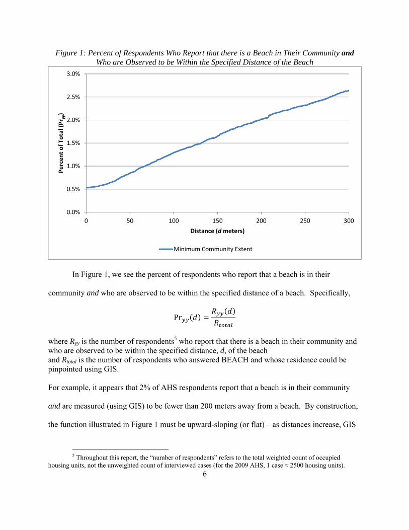
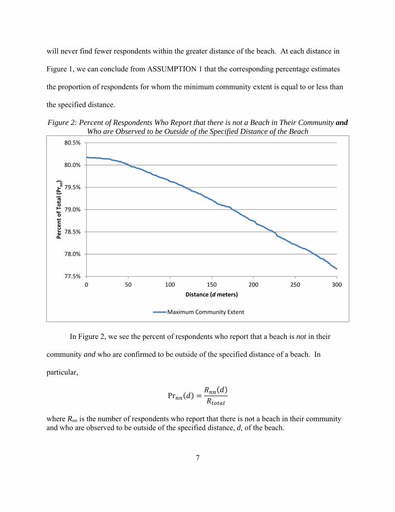
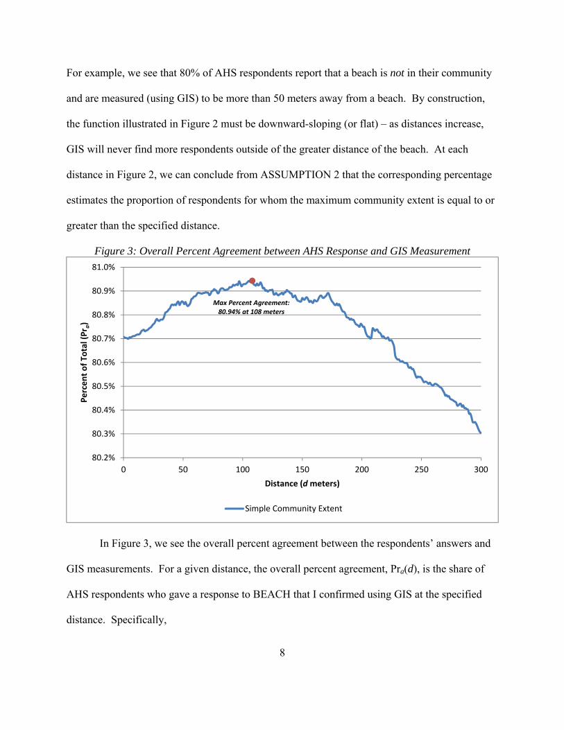
ሻሺ ሻሺ௬௬ൌሻሺPr ௧௧
It is clear from the above equation that the graph in Figure 3 is the vertical summation of the
graphs in Figure 1 and Figure 2 and therefore represents a simple method for combining the
implications of ASSUMPTION 1 and ASSUMPTION 2 At close distances the graph of the
function in Figure 3 seems to slope upward This suggests that as we move away from the
immediate vicinity of AHS households the increase in respondents graphed in Figure 1 is larger
(in absolute terms) than the decrease in respondents graphed in Figure 2 The opposite is true at
the farthest distances where the apparently downward-sloping function indicates that at
increasing distances the increase in respondents graphed in Figure 1 is smaller (in absolute
terms) than the decrease in respondents graphed in Figure 2
The maximum percent agreement is 8094 at a distance of 108 meters and I have
labeled this point in Figure 3 Movements away from the maximum distance will either sacrifice
more respondents graphed in Figure 1 than we gain in Figure 2 (at decreasing distances) or vice
versa (at increasing distances) Therefore using this simple method in which I add together the
findings illustrated in Figure 1 and Figure 2 we might conclude that the typical Americanrsquos
community extent is in the vicinity of 108 meters
9
The Kappa Coefficient
Using a simple method in the previous section I argued that the distance that maximizes
the overall percent agreement marks a point that optimally combines the implications of
ASSUMPTION 1 and ASSUMPTION 2 The main problem with this simple method is that the
overall percent agreement gives too much weight to the respondentrsquos graphed in Figure 2 ndash this
explains why the function in Figure 3 starts decreasing (matching Figure 2) after only 108
meters Since a large majority (805 plusmn0856) of AHS respondents report that they do not
live near a beach a one percent decrease in Figure 2rsquos respondents will be much larger in
absolute terms than a one percent increase in respondents graphed in Figure 1 In other words
changes in Figure 2 are more likely (compared to Figure 1) only because these respondents
comprise a much larger share of the total population
Cohenrsquos kappa coefficient (or simply the kappa coefficient) adjusts the overall percent
agreement and compensates for this imbalance The kappa coefficient calculates the level of
agreement between a pair of Boolean responses or determinations while accounting for the level
of agreement that would occur by chance (Cohen 1960) This statistic is computed using the
following formula
ሻሺെ Pr ሻሺPrൌሻሺߢ ሻሺ1 െ Pr
where Pra(d) is the observed percent agreement at distance d
ሻሺ ሻሺ௬௬ൌሻሺPr ௧௧
6 The ranges presented in this report represent the 95 confidence interval unless otherwise stated Following guidance from the American Housing Survey designers I use replicate weights and Fayrsquos Balanced Repeated Replication (BRR) method of variance estimation (US Dept of Housing and Urban Development 2012)
10
Pre(d) is the percent agreement that is expected to occur by random chance
ሻሺ௬ ሻሺൈሻሺ௬ ሻሺ ቈ
ሻሺ௬ ሻሺ௬௬ൌ ቈ ሻሺPr ௧௧௧௧௧௧
ሻሺ௬ ሻሺ௬௬ൈ ௧௧
Ryy(d) is the number of times that both determinations were positive Ryn(d) is the number of times that the first determination was positive and the second determination was not positive Rny(d) is the number of times that the first determination was not positive and the second determination was positive Rnn(d) is the number of times that both determinations were not positive and Rtotal is the total number determination pairs (Rtotal = Ryy + Ryn + Rny + Rnn)
The kappa coefficient discounts one-sided situations in which both determinations are matched
in the vast majority of cases ndash that is situations in which both answers are almost always ldquoYesrdquo
or both are almost always ldquoNordquo If the observed percent agreement Pr(a) is less than the
expected percent agreement Pr(e) then kappa will be negative In evaluating the level of
agreement Table 1 lists the conventional ranges for the kappa coefficient (Landis amp Koch
1977)
In Table 2 I calculate the kappa coefficient for AHS
respondents who answered BEACH7 For the first example I Table 1 Kappa Coefficient Levels of Agreement Ranges
arbitrarily chose a community extent of 1000 meters We see Poor Slight
Less than 0 000 ndash 020
that 59 million households gave an affirmative answer to Fair Moderate
020 ndash 040 040 ndash 060
BEACH and are GIS-verified to be within 1000 meters of a Substantial Almost Perfect
060 ndash 080 080 ndash 100
beach Similarly 742 million households gave a negative response to BEACH and are GIS-
confirmed to be more than 1000 meters away from a beach However 264 million households
7I conclude from my research that most AHS respondents do not consider ordinary municipal state or federal parks to qualify as a neighborhood feature that pertains to BEACH Maximum kappa coefficients when excluding various combinations of GIS maps of parks (ie including only beaches and shorelines) are always higher than maximum kappa coefficients including various combinations of park maps Therefore the research in the report uses only GIS maps of beaches and shorelines (not parks) when measuring the distance from the respondent to the nearest beach park or shoreline
11
gave a response to BEACH that was contradicted by GIS measurements at 1000 meters At this
distance I calculate the observed percent agreement Pr(a) to be 752 (plusmn078) and the kappa
coefficient to be 01606 (plusmn00161) According to Table 1 the level of agreement between the
GIS measurement and the AHS response for this range of distances is ldquoslightrdquo
In Table 3 and Table 4 I repeat the calculations from Table 2 for 500 meters and 750
meters respectively Of these three distances (500m 750m 1000m) the overall percent
agreement (792 plusmn08) is highest at 500 meters where we also find the largest proportion of
respondents (755) who answered ldquoNordquo to BEACH and whose response at this distance is
verified by GIS8 However we see that the point estimate for the kappa coefficient (01666) is
highest at 750 meters ndash the highest kappa coefficient and the highest percent agreement are not at
the same distance Comparing Table 3 and Table 4 we see that the higher kappa coefficient
results from trading three reported percentage points in the predominant NoNo response
combination for just one more reported percentage point in the less likely YesYes response
combination Hence these examples show how the kappa coefficient discounts one-sided
situations where one combination of AHS responses and GIS measurements overwhelmingly
match
8 By construction the percent of responses in the NoNo combination will always be highest at the closest distances (ie Figure 2) and the proportion of responses in the YesYes combination will always be highest at farthest distances (ie Figure 1)
12
Table 2 AHSGIS cross tabulation of BEACH at 1000m
Table 3 AHSGIS cross tabulation of BEACH at 500m
AHS Response AHS Response
Yes No Total Yes No Total
GIS
Mea
sure
men
t
Yes
5940558 56 (Ryy)
11562050 108 (Ryn)
17502608 164
GIS
Mea
sure
men
t
Yes
3913686 37 (Ryy)
5340813 50 (Ryn)
9254499 87
No
14849758 139 (Rny)
74212141 696 (Rnn)
89061899 836 N
o
16876630 158 (Rny)
80433378 755 (Rnn)
97310008 913
Tot
al 20790316 195
85774191 805
106564507 1000 (Rtotal)
Tot
al 20790316 195
85774191 805
106564507 1000 (Rtotal)
Pr(a) 752 (plusmn08) Pr(a) 792 (plusmn08)
Kappa coefficient 01606 (plusmn00161) Kappa coefficient 01595 (plusmn00161)
Table 4 AHSGIS cross tabulation of BEACH at 750m
Table 5 AHSGIS cross tabulation of BEACH at 790m
AHS Response AHS Response
Yes No Total Yes No Total
GIS
Mea
sure
men
t
Yes
5056267 47 (Ryy)
8463838 79 (Ryn)
13520105 127
GIS
Mea
sure
men
t
Yes
5240055 49 (Ryy)
8971931 84 (Ryn)
14211986 133
No
15734049 148 (Rny)
77310352 725 (Rnn)
93044401 873 N
o
15550261 146 (Rny)
76802260 721 (Rnn)
92352521 867
Tot
al 20790316 195
85774190 805
106564506 1000 (Rtotal)
Tot
al 20790316 195
85774191 805
106564507 1000 (Rtotal)
Pr(a) 773 (plusmn07) Pr(a) 770 (plusmn07)
Kappa coefficient 01666 (plusmn00158) Kappa coefficient 01675 (plusmn00158)
13
The Maximum Kappa Coefficient and the Derived Community Extent
Table 5 shows the housing unit estimates and the kappa coefficient at 790 meters and in
Figure 4 we see that the kappa coefficient for all AHS respondents is maximized near this
distance The kappa coefficient at 790 meters 01675 is the largest value resulting from an
algorithm that I developed to recursively search the range of all possible distances at 10-meter
intervals for the maximum kappa coefficient9 This algorithm executed these following steps
Step 1 Identify the respondents who are at the minimum and maximum distances from a beach or shoreline ndash this is the range For all AHS respondents the range of distances from their residence to the nearest beach or shoreline is 0 meters to over 80000 meters (about 50 miles)
Step 2 Evenly divide the range into 200 segments and calculate the kappa coefficient at each of these distances (rounded to the nearest multiple of 10)
Step 3 Of these 200 distances identify the maximum kappa coefficient and calculate the distances (rounded to the nearest multiple of 10) that are 25 segments (125 of the range) fewer than and 25 segments greater than this kappa-maximizing distance ndash this is the new range
Step 4 If the new range is greater than 200 meters repeat Step 2 and Step 3
Step 5 If the new range is 200 meters or less calculate the kappa coefficient at each distance (rounded to the nearest multiple of 10)
Step 6 Identify the distance with the maximum kappa coefficient within the new range this is the maximum kappa and maximizing distance reported in this research
In this report I will refer to the distance that maximizes kappa as the derived community
extent This search function is effective because the graph of the kappa coefficient with respect
to distance generally increases reaches a peak and then generally decreases However the
function is not strictly concave a local maximum is usually not the global maximum and the
9 Due to limited computer processing resources the recursive search function only calculated and compared kappas at distances that were multiples of ten I also round standard errors and confidence intervals for these maximizing distances to the nearest multiple of ten
14
search function can differentiate between the two This pattern is evident in Figure 4 where we
also see that the graph of kappa coefficients is flat near the maximum point Table 8 confirms
that the 95 confidence interval for this derived community extent is 520 meters to 1060 meters
For context I note that if a neighborhood extends 520 m ndash1060 m in all directions from the
respondentrsquos home then his or her community is a circle that encompasses 085ndash353 km2 (210ndash
872 acres) in total area
Figure 4 Kappa Coefficients for Distances between 0 and 2000 meters
Kap
pa
018
015
012
009
006
003
000
Max Kappa 01675 at 790 m
0 200 400 600 800 1000 1200 1400 1600 1800 2000
Distance (d meters)
Kappa Coefficient 95 Confidence Interval
In Table 6 I derive the average extent of the smallest tabulation areas produced by the
US Census Bureau zip code tabulation areas (ZCTAs) census tracts census block groups and
census blocks Each mean derivation starts by dividing the total area of the United States (ie
the total area of 50 states plus the District of Columbia) by the number of tabulation areas that
the Census Bureau defines within the area Next I derive the average radius or extent of each
15
tabulation area under various assumptions For example if we assume that ZCTAs are best
represented by circles then the mean radius of the ZCTA is 8559 meters Under this
assumption the mean ZCTA radius is 8 to 16 times longer than the derived community extent
Table 6 also includes derivations for the median extents of the US Census Bureaursquos
smallest tabulation areas under the same assumptions All of the tabulation areas include regions
that encompass extremely large areas in the least populated parts of the United States ndash for
example each of the five largest census blocks (all in Alaska) is larger than Connecticut (which
contains 67578 census blocks) These massive areas skew the mean calculation and make the
median a better measure of central tendency Table 6 shows that if the median zip code were a
circle then its radius would be 5533 meters which is 5 to 11 times longer than the derived
community extent This implies that researchers who use zip codes to account for neighborhood
effects are overestimating the range of these reactions
16
Figure 5 Census Blocks (white outline) Census Block Groups (blue outline) and Census Tracts (red outline) in Maryland the District of Columbia
US Census Bureau HQ
Source TIGERLine Shapefiles 2012 US Census Bureau Geography Division
However it is not realistic to assume that circles are the best representation of the
smallest tabulation areas Census blocks are generally bounded by streets or roads which means
that their edges are usually more straight than rounded Since all of the larger tabulation areas
are comprised of census blocks their edges are also frequently straight Figure 5 which is a map
of a portion of Southeast Washington DC and Prince Georgersquos County MD illustrates typical
census tabulation areas On this map I outline census blocks in white census block groups in
blue and census tracts in red
In Table 6 I also calculate the shortest and longest extents of a median-sized tabulation
area assuming that it is a square For census blocks the shortest extent (from the center of the
square to the midpoint of any edge) under this assumption is 84 meters and the longest extent
17
(from the center of the square to any corner) is 119 meters Compared to the derived community
extent (between 520 meters and 1060 meters) this implies that researchers who use census
blocks to control for neighborhood effects are underestimating the range of these responses
Relative to the US Census Bureaursquos tabulation areas the best approximation of the derived
community extent is between one and two median-sized census block groups Since the median
census block group contains 532 housing units this further implies that the typical American
community includes 500ndash1000 homes
18
Table 6 Average Areas and Derived Extents of US Census Bureau Tabulation Areas
Figure Equation Zip Code Tab Area (ZCTA)
Census Tracts Block Groups Census Blocks
Count 32990 73057 217740 11078297
Mea
n
Area (square meters)dagger
Housing unitsDagger
Derived radius (meters)
Derived extent (meters) if the area is a square and the length extends to the nearest point on the square Derived extent (meters) if the area is a square and the length extends to the farthest point on the square
ܣݎඨݎ ൌ ߨ
ܣݎඨݎ ൌ 4
ܣݎඨݎ ൌ 2
230135677 134600885 45161830 887640 3991 1803 605 12
8559 6546 3791 532
7585 5801 3360 471
10727 8204 4752 666
Med
ian
Area (square meters) Housing units
Derived radius (meters)
Derived extent (meters) if the area is a square and the length extends to the nearest point on the square Derived extent (meters) if the area is a square and the length extends to the farthest point on the square
ܣݎඨݎ ൌ ߨ
ܣݎඨݎ ൌ 4
ܣݎඨݎ ൌ 2
96160479 5206992 1377784 28373 NA 1706 532 2
5533 1287 662 95
4903 1141 587 84
6934 1614 830 119
dagger The total area of the 50 US States (plus Washington DC) is 9833537 km2 ZCTAs do not cover all areas of the United States the total area of ZCTAs is 7592176 km2 Dagger The 2010 US Census Bureau count of housing units in the 50 US States (plus Washington DC) is 131704730 Source See Appendix B
19
Maximum Kappa Coefficients and Derived Community Extents for Various Demographic and Socioeconomic Groups
Table 8 presents the derived community extents and maximum kappa coefficients for
various demographic and socioeconomic groups Using replicate weights (see footnote 6) I
construct 95 confidence intervals around these estimates and I have included these ranges in
Table 8 as well As explained in the previous section the kappa coefficient for AHS respondents
in all occupied housing units is maximized at a distance of 790 meters from the respondentrsquos
home However if the AHS sample were repeatedly drawn this derived community extent
would range between 520 meters and 1060 meters 95 of the time This finding is consistent
with other research that shows the spillover effect of foreclosures on neighboring property values
in Chicago is not statistically significant beyond 900 meters (Lin Rosenblatt amp Yao 2009)
The maximum kappa coefficient is 01675 (plusmn 00158) and the range for these maximum kappa
values indicates that there is a slight level of agreement between GIS measurements and AHS
respondents regarding the presence or absence of beaches within the derived community extent
Other noteworthy findings from Table 8 include
The derived community extent is smaller for renters than for owners but this difference is not statistically significant The maximum kappa coefficient for owners is higher than renters and this difference is statistically significant at the 90 confidence level
The derived community extent is not statistically different across different racial groups The maximum kappa coefficient is higher for White (alone) householders than for householders who are African-American (alone) Asian (alone) and Hispanic or Latino (any race) and there is evidence for this difference at the 95 confidence level
Respondents in buildings with 50 or more units in the structure live in smaller communities than those in ordinary single-family homes and this difference is statistically significant at the 90 level The difference in the kappa coefficient between any pair of structure types is not statistically significant
20
The derived community extent for residents in condominiums is small in comparison to the population in all occupied units The point estimate for the maximum kappa coefficient for residents of these condo communities is higher than the point estimates for all other demographic and socioeconomic indicators analyzed in this report and the difference is usually statistically significant For context Table 7 includes the weighted housing unit counts that contribute to this relatively high kappa calculation
Residents in older homes tend to live in Table 7 AHSGIS cross tabulation of larger communities The Pearson BEACH for condo residents at 410m correlation coefficient between the midpoints of the age ranges of homes and the point estimates of the derived community extents in Table 8 is 05465 p-value=00432 However none of the differences between any pair of age ranges is statistically significant
The differences in the derived community extent among residents who live inside central cities within suburbs and outside metro areas are not statistically significant However there is less agreement about the presence or absence of beaches in central cities than outside of MSAs based on the maximum kappa coefficient
Communities in the Midwest are larger than Southern communities and this difference is evident at the 95 confidence level Agreement on the presence or absence of beaches within the derived community extent is higher in the South than in every other region of the country and this difference is also statistically significant at the 95 level
AHS Response
Yes No Total
GIS
Mea
sure
men
t
Yes
384460 62
(Ryy)
373155 60
(Ryn)
757615 122
No
721294 116
(Rny)
4733251 762
(Rnn)
5454545 878
Tot
al 1105754 178
5106406 822
6212160 1000
(Rtotal)
Pr(a) 824 (plusmn16) Kappa coefficient 03132 (plusmn00499)
There is no statistically significant difference in the derived community extent or maximum kappa values among respondents who live in places with various populations
21
Table 8 Maximum Kappa Coefficient and the Derived Community Extent for Various Characteristics10
Characteristic
Derived Community Extent (m) Maximum Kappa Coefficient Point Est
Std Error
Lower Bound
Upper Bound
Point Est
Std Error
Lower Bound
Upper Bound
All occupied units
Tenure
790 140 520 1060 01675 00080 01518 01833
Owner occupied 820 140 540 1100 01822 00107 01613 02032 Renter occupied
Race and Hispanic Origin
760 130 510 1010 01441 00105 01235 01646
White alone 680 140 410 950 01802 00094 01619 01986 Non-Hispanic 680 130 430 930 01890 00102 01689 02091 Hispanic 1410 860 -280 3100 01216 00181 00861 01570
Black alone 960 240 480 1440 00937 00167 00609 01264 Non-Hispanic 960 330 310 1610 00871 00167 00544 01197 Hispanic 520 430 -320 1360 02802 01101 00645 04960
American Indian or Alaska Native alone 750 410 -60 1560 01569 00837 -00071 03210 Asian alone 360 650 -910 1630 00765 00288 00200 01330 Pacific Islander alonedagger 3290 4470 -5470 12050 01495 01571 -01584 04573 Two or more races 1410 890 -330 3150 02472 00568 01359 03585 Hispanic or Latino (any race)Dagger
Units in Structure
1340 1040 -710 3390 01187 00184 00825 01548
1 detached 820 60 700 940 01718 00107 01508 01928 1 attached 800 240 330 1270 01310 00264 00794 01827 2 to 4 460 640 -800 1720 01502 00196 01118 01886 5 to 9 740 210 330 1150 01376 00311 00767 01985 10 to 19 750 170 420 1080 02006 00293 01433 02580 20 to 49 880 370 160 1600 01594 00312 00983 02205 50 or more 430 160 110 750 02224 00282 01671 02776 Manufacturedmobile home or trailer
Cooperatives and Condominiums
420 310 -190 1030 02974 00638 01724 04225
Cooperatives 240 630 -990 1470 02472 00748 01006 03939 Condominiums
Year Structure Built
410 120 170 650 03132 00254 02635 03630
2005 to 2009 550 1120 -1640 2740 01609 00437 00753 02465 2000 to 2004 590 80 440 740 01916 00297 01333 02498 1995 to 1999 760 480 -190 1710 01831 00285 01272 02390 1990 to 1994 850 110 640 1060 02746 00393 01976 03515 1985 to 1989 780 300 190 1370 02246 00252 01753 02740 1980 to 1984 700 220 260 1140 02066 00287 01502 02629
10 The characteristics and categories in Table 8 match the definitions and selection criteria used in Table 2shy1 Introductory CharacteristicsmdashOccupied Units of American Housing Survey for the United States 2009 Current Housing Reports (March 2011)
22
Table 8 Maximum Kappa Coefficient and the Derived Community Extent for Various Characteristics10
Characteristic
Derived Community Extent (m) Maximum Kappa Coefficient Point Est
Std Error
Lower Bound
Upper Bound
Point Est
Std Error
Lower Bound
Upper Bound
1975 to 1979 550 190 180 920 01705 00228 01258 02152 1970 to 1974 780 220 360 1200 02124 00223 01688 02561 1960 to 1969 1180 710 -220 2580 01491 00170 01158 01824 1950 to 1959 850 640 -390 2090 01307 00176 00962 01651 1940 to 1949 1070 280 510 1630 01432 00235 00971 01893 1930 to 1939 710 150 410 1010 01418 00266 00896 01940 1920 to 1929 1430 1100 -720 3580 01030 00259 00522 01538 1919 or earlier
MetropolitanNonmetropolitan Areas
770 280 210 1330 01604 00225 01163 02044
Inside metropolitan statistical areas 800 110 580 1020 01557 00075 01410 01704 In central cities 790 180 430 1150 01276 00108 01064 01488 Suburbs 640 220 200 1080 01725 00100 01528 01922
Outside metropolitan statistical areas
Regions
750 210 330 1170 02221 00300 01634 02808
Northeast 680 190 300 1060 01501 00136 01235 01767 Midwest 1350 300 750 1950 01488 00180 01136 01840 South 500 80 340 660 02312 00194 01931 02692 West
Place Size
790 90 610 970 01427 00225 00986 01868
Fewer than 2500 persons 860 330 220 1500 01888 00392 01120 02656 2500 to 9999 persons 840 180 480 1200 01514 00205 01112 01917 10000 to 19999 persons 1400 950 -450 3250 01031 00231 00578 01483 20000 to 49999 persons 680 200 280 1080 01225 00164 00903 01547 50000 to 99999 persons 740 330 100 1380 01264 00190 00892 01635 100000 to 249999 persons 790 310 190 1390 01695 00251 01202 02188 250000 to 499999 persons 500 400 -290 1290 00604 00214 00185 01023 500000 to 999999 persons 1190 20 1160 1220 01669 00328 01026 02311 1000000 persons or more 430 1080 -1690 2550 01043 00185 00681 01405 dagger Native Hawaiian and Other Pacific Islander Dagger Because Hispanics may be any race data can overlap slightly with other groups Most Hispanics report
themselves as White but some report themselves as Black or in other categories
23
An Alternative Method for Deriving Neighborhood Size
In previous sections of this report I derived the community extent by comparing the
incidence of AHS respondents who report that a beach or shoreline is in their neighborhood with
the GIS-measured distance to the nearest body of water I defined this derived community extent
as the distance at which the level of agreement (measured by the kappa coefficient) between the
AHS response and the GIS measurement is maximized However this distance is difficult to
interpret For example it is convenient to assume that the derived community extent is the same
distance in every direction from the respondent but this implies that each neighborhood is circle
with its center at the respondentrsquos home Alternatively for the sake of analytical ease we might
imagine that each neighborhood is a square and the derived community extent measures the
distance to the nearest or farthest points of the square but this assumption also fails to capture
the unlimited variety of neighborhood shapes and sizes
In reality no community in America is a perfectly symmetric shape with a smooth
boundary centered on an AHS respondent Actual communities are usually simple polygons
with borders formed by well-established often-winding landmarks like highways rivers and
streams political jurisdictions etc Not incidentally the US Census Bureau uses many of these
same boundaries to help mark the edges of census blocks block groups tracts and ZCTAs11
This makes these tabulation areas ideal proxies for actual neighborhoods In this section I will
derive an estimate of community size that takes advantage of the potential alignment between
actual neighborhoods and tabulation areas
11 In the hierarchy of physical features that the US Census Bureau uses to create the boundaries of census blocks the highest priority shapes are (in order) water areas named and unnamed roads and political jurisdictions (US Census Bureau 1994)
24
Similar to the approach that I described in the previous sections (which I will refer to as
Method A) I will compare the incidence of AHS respondents who report that a beach or
shoreline is in their community with the GIS-determined presence or absence of a significant
body of water within census tabulation areas Then I will identify the tabulation areas (grouped
by size) that maximize the level of agreement (measured by kappa) between the AHS response
and the GIS observation I will call this second approach Method B12
As an example see Figure 6 which is a map identifying census blocks (white outline)
block groups (blue outline) and tracts (red outline) in Miami Beach FL For the sake of this
example I have pinpointed two
hypothetical AHS respondents Imagine
that Respondent A answered ldquoYesrdquo to
BEACH Since neither her census block
nor block group border the ocean these
tabulation areas obviously cannot outline
the area that she would say is in her
community ndash I assume that these areas are
too small If her neighborhood is
coextensive with a census tabulation area
then it must match either her census tract or
ZCTA (none of Miami Beachrsquos five zip
codes is landlocked)
Figure 6 Census Blocks (white outline) Census Block Groups (blue outline) and Census Tracts
(red outline) in Miami Beach FL
Source TIGERLine Shapefiles 2012 US Census Bureau Note I chose the location of Respondent A and Respondent B for the purpose of this illustration These locations may or may not pinpoint the addresses of actual AHS respondents
12 I acknowledge and thank Charles A Bee my colleague at the US Census Bureau for proposing Method B
25
Alternatively consider Respondent B who answered ldquoNordquo to BEACH Since this
respondentrsquos block group tract and ZCTA border the ocean I conclude that these tabulation
areas are too big to match this respondentrsquos conception of his community If a tabulation area
happens to be coterminous with this respondentrsquos community then it must be his census block13
When creating tabulation areas the US Census Bureau respects many of the same natural and
political boundaries that outline actual communities which means that a tabulation area might
share the same physical space as real neighborhoods and subdivisions However this will only
be true for AHS survey respondents when their answer to BEACH agrees with the GIS-
determined presence or absence of a body of water in the tabulation area My objective in
Method B is to identify the size of tabulation areas that maximizes the level of agreement
between the AHS response and the GIS determination
Table 9 details the results of this analysis which proceeded along these steps
Step 1 Locate every AHS respondent who answered BEACH within his or her census block block group tract and ZCTA and create an expanded AHS sample that includes duplicate entries for each of these four tabulation areas
Step 2 Sort this expanded sample by the size of the tabulation area and divide this dataset into 120 classes having roughly the same weighted number of housing units (not the unweighted number of cases) For the sample of all occupied housing units I find that the average area of the smallest class is approximately equal to the playing surface of an American football field and the average area in the largest class is larger than the cities of Los Angeles and Chicago combined The median-sized class is the same size as New York Cityrsquos Central Park
Not surprisingly the smallest classes are entirely composed of census blocks and the largest classes are dominated by ZCTAs The derived radius in Table 9 is the distance from the center of the average area to its edge assuming that its shape is a circle
ݒݎ ݏݑݎ ඥൌݎݒ ݎߨ
13 Method B separately considers four tabulation areas (blocks block groups tracts and ZCTAs) as potential neighborhoods that align with the respondentrsquos own community therefore this analysis counts each interview as many as four times
26
Step 3 Determine the AHS ResponseGIS Determination combination of weighted household counts within each class Notice the pattern of disagreement between the AHS Response and the GIS Determination in Table 9 Where there is disagreement in the smallest areas it is overwhelmingly because the AHS respondent gave an affirmative answer to BEACH but GIS determined that the tabulation area does not contain a large body of water Disagreement in the largest areas is primarily due to the AHS respondent giving a negative response to BEACH where GIS determined that there is a body of water within the tabulation area
Step 4 Calculate the percent agreement and the kappa coefficient for each class and identify the maximum kappa coefficient For the sample of all occupied housing units the kappa coefficient is maximized in the 58th class The average size for the 58th class is comparable in area to the primary airport in Baton Rouge LA (BTR) Buffalo NY (BUF) or Santa Barbara CA (SBA) The derived radius for this class (987 meters) implies that these tabulation areas fit within the 95 confidence interval of the derived community extent that I calculated earlier in this report using Method A (between 520 and 1060 meters)
27
5
10
15
20
25
30
35
40
45
50
55
60
65
Table 9 Selected Statistics by Class Using Method B for All Occupied Housing Units
Class Housing Units Average Area
(m2) Derived
Radius (m) Blocks Block
Groups Tracts ZCTAs AHS ResponseGIS Determination Percent
Agree Kappa Coeff
Smooth KappaYesYes NoYes YesNo NoNo
1 3549533 5142 40 100 0 0 0 17531 28741 926405 2576856 731 00108 2 3552921 8884 53 100 0 0 0 11407 15341 837083 2689089 760 00116 3 3547052 11272 60 100 0 0 0 33968 16693 721923 2774468 792 00590 00252 4 3554486 13436 65 100 0 0 0 21007 21252 841768 2670459 757 00243 00285
3552276 15586 70 99 1 0 0 17672 21038 815607 2697959 764 00201 00304 6 3551547 17589 75 98 2 0 0 15950 11616 718263 2805718 794 00273 00333 7 3550045 19612 79 99 1 0 0 16315 19363 766038 2748329 779 00211 00345 8 3553198 21544 83 98 2 0 0 41929 14723 731182 2765364 790 00735 00455 9 3551292 24046 87 97 3 0 0 29528 36287 831413 2654064 756 00303 00435
3551485 27157 93 98 2 0 0 37560 14082 659439 2840404 810 00753 00439 11 3551209 30675 99 96 4 0 0 18891 35111 766231 2730976 774 00171 00307 12 3550409 34775 105 95 5 0 0 18599 31324 689407 2811079 797 00234 00349 13 3550923 39351 112 94 6 0 0 16088 41411 783533 2709892 768 00076 00366 14 3550922 44748 119 93 7 0 0 30454 33622 644825 2842020 809 00511 00536
3550699 52126 129 91 9 0 0 48949 28066 691714 2781970 797 00837 00791 16 3552516 61140 140 89 11 0 0 59117 62104 588006 2843289 817 01023 00957 17 3552379 71907 151 86 12 1 0 75792 17079 628388 2831121 818 01510 01146 18 3551247 85378 165 85 14 1 0 52883 62181 584993 2851190 818 00905 01233 19 3549964 101944 180 80 18 2 0 71998 57558 529224 2891184 835 01457 01308
3552434 121817 197 73 23 4 0 77653 45872 666561 2762349 799 01269 01200 21 3550452 144179 214 67 24 10 0 77543 66316 567192 2839400 822 01397 01210 22 3553450 166163 230 53 29 18 0 67841 76925 643539 2765145 797 00974 01078 23 3550113 189155 245 57 29 14 0 63528 98745 563156 2824683 814 00954 01127 24 3551664 217505 263 53 36 10 0 60019 82909 647486 2761250 794 00795 01110
3550524 248991 282 47 44 8 0 117107 118275 635508 2679633 788 01513 00998 26 3552455 281947 300 47 46 8 0 90338 127464 549571 2785082 809 01312 00987 27 3549955 316794 318 36 54 10 0 43759 95979 654810 2755406 789 00415 01117 28 3553038 349773 334 39 53 9 0 73295 99854 659947 2719941 786 00900 00964 29 3546341 387887 351 33 55 12 0 93550 89616 596179 2766996 807 01445 00920
3556304 430156 370 35 54 11 0 70813 133104 627222 2725165 786 00749 01099 31 3549869 474275 389 27 61 12 0 99758 138400 660180 2651531 775 01089 01101 32 3552438 518186 406 28 60 11 0 129595 191990 623341 2607512 770 01310 01032 33 3552694 566885 425 25 60 15 0 85801 144968 634297 2687628 781 00910 01061 34 3551071 616740 443 24 61 14 0 86335 129423 596068 2739245 796 01101 01058
3550959 658236 458 18 65 17 0 66314 121490 557958 2805198 809 00893 01172 36 3551307 705964 474 23 60 16 2 106511 183441 611045 2650310 776 01077 01229 37 3552382 765617 494 25 60 15 0 165369 169155 620527 2597331 778 01879 01177 38 3549990 827769 513 22 59 18 1 118613 220636 564617 2646125 779 01196 01177 39 3552614 894129 533 23 54 23 1 95995 239569 540449 2676601 780 00842 01177
3551623 965993 555 22 52 25 1 106703 242612 573207 2629101 770 00890 01031 41 3548641 1036220 574 20 52 25 2 106262 251395 498179 2692804 789 01079 01150 42 3553031 1116167 596 18 52 29 1 120296 256503 531943 2644289 778 01148 01160 43 3550334 1200484 618 19 49 31 1 160240 259821 496580 2633693 787 01791 01128 44 3552157 1279055 638 14 43 43 1 78997 184194 520645 2768321 802 00893 01158
3552325 1346817 655 18 45 37 1 98402 257313 561683 2634927 769 00731 01118 46 3551123 1437011 676 16 47 35 2 140243 317102 503020 2590759 769 01228 01135 47 3550151 1543722 701 15 40 42 3 119429 284901 546865 2598957 766 00948 01103 48 3552934 1655841 726 18 39 41 3 193835 354638 456246 2548216 772 01874 01270 49 3551655 1769588 751 15 42 41 2 135489 375139 551269 2489758 739 00735 01101
3551252 1892028 776 14 36 45 4 163310 283308 532765 2571870 770 01566 01210 51 3551782 2016421 801 13 36 49 2 83678 289215 553738 2625152 763 00382 01074 52 3550971 2158234 829 15 35 47 3 197042 389242 514983 2449704 745 01495 01072 53 3550921 2294293 855 14 36 46 4 182061 443957 491019 2433884 737 01194 01017 54 3550634 2444877 882 13 34 50 3 136112 364328 570258 2479936 737 00725 01160
3552465 2578116 906 13 26 58 3 110243 207500 519975 2714747 795 01290 01053 56 3549962 2691009 926 12 29 55 5 162622 401394 508137 2477809 744 01097 01254 57 3552802 2862014 954 13 30 45 11 174894 499843 474628 2403438 726 00957 01339 58 3551623 3063461 987 11 33 53 3 259892 448828 425184 2417718 754 02199 01330 59 3551447 3292028 1024 10 32 51 7 176091 492980 436931 2445446 738 01153 01207
3550938 3527420 1060 12 27 54 7 214756 507186 492713 2336283 718 01242 01255 61 3551724 3772725 1096 9 27 54 9 172397 536531 552427 2290369 693 00484 01247 62 3550978 4032666 1133 13 26 48 13 203856 578949 414166 2354006 720 01198 01328 63 3551809 4350033 1177 6 28 58 8 266187 498220 398058 2389345 748 02157 01432 64 3550740 4683853 1221 8 29 52 11 284377 673330 402344 2190688 697 01557 01688
3552374 5060758 1269 10 27 53 10 244656 467135 473685 2366898 735 01764 01788 66 3549533 5418256 1313 10 25 52 14 286381 605347 417333 2240472 712 01765 01659
28
Table 9 Selected Statistics by Class Using Method B for All Occupied Housing Units
Class Housing Units Average Area
(m2) Derived
Radius (m) Blocks Block
Groups Tracts ZCTAs AHS ResponseGIS Determination Percent
Agree Kappa Coeff
Smooth KappaYesYes NoYes YesNo NoNo
67 3552450 5829364 1362 8 28 46 18 330254 729755 392401 2100040 684 01696 01563 68 3550654 6307479 1417 9 27 45 20 298971 733850 386079 2131755 685 01511 01522 69 3552106 6836571 1475 7 26 45 23 331254 823568 450434 1946850 641 01080 01400 70 3550649 7428593 1538 5 28 46 21 334822 772439 393342 2050045 672 01560 01230 71 3552884 8022909 1598 6 27 43 24 307469 805794 419158 2020463 655 01153 01061 72 3550282 8746589 1669 5 24 39 33 276615 847487 412779 2013401 645 00847 01104 73 3552476 9521904 1741 4 28 35 32 288356 884485 442074 1937561 627 00664 00949 74 3550191 10335667 1814 4 26 40 30 326236 821400 401035 2001520 656 01298 01045 75 3552858 11246662 1892 4 25 37 34 273267 849737 420544 2009310 642 00783 01177 76 3551343 12258202 1975 2 26 33 39 425518 832735 428230 1864860 645 01633 01277 77 3550172 13267068 2055 2 22 34 43 387269 916748 358601 1887554 641 01509 01250 78 3550416 14341750 2137 4 19 32 45 356377 950065 375368 1868605 627 01162 01309 79 3553358 15433165 2216 3 21 30 47 334677 827519 434636 1956526 645 01163 01202 80 3551771 16553973 2295 1 19 27 53 297469 872296 376629 2005377 648 01078 01241 81 3551324 17685221 2373 1 22 24 53 393163 953544 420005 1784611 613 01099 01039 82 3548644 18882424 2452 1 19 24 56 456600 1023338 309802 1758905 624 01705 00997 83 3553685 20165250 2534 1 19 26 55 286909 1056413 442251 1768113 578 00148 01089 84 3550143 21682064 2627 1 20 22 57 437643 1246848 311765 1553887 561 00953 01115 85 3552462 23304432 2724 1 18 22 59 404554 987477 323458 1836973 631 01540 00993 86 3550183 24994782 2821 1 19 27 52 350843 1019879 315348 1864112 624 01230 01155 87 3552672 26941195 2928 1 20 20 60 364671 1143301 287129 1757570 597 01096 01093 88 3551524 28958104 3036 1 20 22 57 346307 1167215 286078 1751924 591 00956 01026 89 3551884 31071411 3145 2 23 20 55 398039 1239941 346940 1566964 553 00643 00817 90 3551569 33455115 3263 0 18 23 59 445577 1189596 300389 1616006 580 01206 00890 91 3550935 35996274 3385 0 20 21 59 316312 1420421 297528 1516674 516 00184 00834 92 3548854 38862404 3517 0 24 21 55 451228 1174938 264959 1657728 594 01460 00901 93 3554147 42281507 3669 0 18 20 61 438036 1445165 270709 1400238 517 00679 00885 94 3551464 46127146 3832 0 20 26 54 430780 1469658 204898 1446127 528 00977 01079 95 3551126 49796707 3981 0 22 25 53 510877 1482977 208485 1348786 524 01123 00989 96 3550691 54034258 4147 0 21 22 57 426235 1350567 220503 1553386 558 01155 01089 97 3552568 58703124 4323 0 19 24 57 376788 1509698 155945 1510138 531 01013 01042 98 3548662 63743436 4504 0 20 23 56 472273 1448430 197442 1430518 536 01177 01059 99 3553592 69209181 4694 0 19 25 56 437596 1574915 208560 1332520 498 00744 01045
100 3551945 75521187 4903 0 17 22 60 447788 1509094 157397 1437665 531 01207 00940 101 3550885 82706555 5131 0 15 26 59 498599 1550150 183015 1319122 512 01084 00767 102 3549164 89896798 5349 0 18 27 55 395309 1744193 178600 1231061 458 00488 00830 103 3552572 98293652 5594 0 19 30 51 417768 1628509 255052 1251244 470 00311 00740 104 3551369 108566221 5879 0 17 22 61 403581 1559348 143529 1444911 521 01062 00703 105 3551784 118958192 6154 0 16 29 56 418806 1573908 198392 1360677 501 00757 00768 106 3550025 130175425 6437 0 13 19 67 512183 1875600 104195 1058048 442 00897 00858 107 3552656 143724330 6764 0 9 27 64 402556 1476498 217264 1456339 523 00811 00797 108 3551029 158891060 7112 0 14 24 62 476122 1683637 180310 1210960 475 00762 00839 109 3552285 177878083 7525 0 8 29 63 415489 1736032 143513 1257251 471 00757 00825 110 3550482 195015323 7879 0 12 23 66 501089 1474112 235222 1340059 519 00967 00772 111 3552926 216936651 8310 0 6 25 69 492306 1829413 126387 1104820 450 00826 00741 112 3550120 244642836 8825 0 9 31 60 426550 1836280 152559 1134731 440 00546 00581 113 3552101 277539297 9399 0 4 26 69 515254 2049019 102051 885778 394 00608 00562 114 3551401 311686969 9961 0 5 27 68 421994 2285270 138406 705731 318 -00043 00366 115 3551820 351316076 10575 0 4 27 69 447909 1733050 136002 1234859 474 00873 00512 116 3550224 397550515 11249 0 5 18 76 479499 2017298 226149 827278 368 -00152 00356 117 3552767 458675178 12083 0 5 28 67 493939 1607957 127214 1323657 512 01272 00250 118 3549890 562730050 13384 0 6 29 65 477492 2113850 202977 755571 347 -00169 -00214 119 3551233 793477243 15893 0 5 26 69 443966 2446500 189440 471327 258 -00574 120 3553188 2217410809 26567 0 9 39 52 517930 2200827 371238 463192 276 -01446
I have highlighted the 58th class where the kappa coefficient is maximized
29
Figure 7 Kappa Coefficients Using Method B
03 Kap
pa
02
01
00
‐01
‐02
Max Kappa 02199 at 1064862 m2
Size (m2) of Tabulation Area
Kappa Coeff Smooth Kappa 95 Confidence Interval
Figure 7 illustrates the data that I have calculated in Table 9 In this figure I plot kappa
coefficients on the vertical axis and the average size of the tabulation area in square meters on
the horizontal axis Notice that the horizontal axis is a logarithmic (base 10) scale ndash each tick
mark indicates an average area that is ten times larger than the previous tick mark The blue
points plotted in Figure 7 are the kappa coefficients calculated in Table 9 The red ldquosmooth
kappardquo line traces a rolling average of five kappa coefficients
where i is a class number between 3 and ሻାଶhellip ଶሺൌ ݐݏ
118 This smooth kappa line illustrates a clear pattern ndash the kappa coefficients for the smallest
and largest tabulation areas are generally low and the peak kappa coefficients occur in midshy
range tabulation areas I will refer to the class of tabulation areas where kappa is maximized as
the derived community area Using replicate weights I find that the 95 confidence interval for
30
the derived community area of all occupied housing units using Method B is 370399 m2 to
25339614 m2 I indicate this confidence internal by the shaded region of Figure 7 If these
upper and lower threshold areas were circles then the derived radius for this range would be 343
m to 2840 m which fully overlaps the derived community extent that I previously calculated
using Method A (520 m ndash 1060 m)
I repeat Method B for the same demographic and socioeconomic groups that I analyzed
using Method A in Table 8 and I present these findings in Table 10 Comparing the two tables I
find no statistically significant differences between any of the derived community extents (of
Method A) and the derived community areas (of Method B) This conclusion assumes that the
shape of the derived community area is a circle and the derived radius measures the distance
from the AHS respondentrsquos home to the edge of his or her community Under this assumption
there is no subpopulation analyzed in Table 8Table 10 in which the confidence intervals do not
overlap at the standard levels for statistical significance
Additionally the confidence intervals using Method B are wider than the confidence
intervals using Method A for all 50 of the subpopulations analyzed in Table 8Table 10 In 35
out of the 50 subpopulations the 95 confidence interval that I derived using Method B
completely overlaps (ie has a smaller lower bound and a larger upper bound than) the 95
confidence interval using Method A Based on these observations I conclude that Method A
produces more precise estimates of community size than Method B
31
Table 10 Alternate Maximum Kappa Coefficient and the Derived Community Area for Various Characteristics14
Characteristic
Derived Community Area (m2) Maximum Kappa Coefficient Point
Est Std
Error Lower Bound
Upper Bound
Point Est
Std Error
Lower Bound
Upper Bound
All occupied units
Tenure
Owner occupied Renter occupied
Race and Hispanic Origin
White alone Non-Hispanic Hispanic Black alone Non-Hispanic HispanicAmerican Indian or Alaska Native alone Asian alone Pacific Islander alonedagger
Two or more races Hispanic or Latino (any race)Dagger
Units in Structure
1 detached 1 attached 2 to 4 5 to 9 10 to 19 20 to 49 50 or more Manufacturedmobile home or trailer
Cooperatives and Condominiums
Cooperatives Condominiums
Year Structure Built
2005 to 2009 2000 to 2004 1995 to 1999 1990 to 1994 1985 to 1989 1980 to 1984
64862 04682 55686 74038
66402 08580 49586 83218 64826 11143 42987 86665
66866 10974 45358 88374 62098 08608 45226 78971 67342 09721 48288 86395 58067 18100 22591 93542 60826 11314 38650 83002
ndash ndash ndash ndash ndash ndash ndash ndash
62825 10546 42156 83495 ndash ndash ndash ndash ndash ndash ndash ndash
56016 18792 19185 92847
66446 08278 50222 82669 59507 07854 44114 74901 58835 08562 42055 75616 70896 19744 32198 109594 56009 09683 37030 74987 63451 14238 35545 91357 51190 10379 30847 71533 63190 14964 33861 92519
ndash ndash ndash ndash 54258 13559 27682 80834
67932 13098 42260 93603 66104 20588 25751 106456 60937 12626 36190 85684 48626 42065 -33820 131072 64832 25503 14846 114818 65294 09198 47266 83323
02199 00312 01588 02810
02483 00399 01701 03265 02630 00567 01519 03741
02287 00325 01651 02923 02331 00397 01552 03109 04153 01103 01992 06315 03404 00849 01741 05068 03308 01041 01268 05348
ndash ndash ndash ndash ndash ndash ndash ndash
03043 03276 -03378 09464 ndash ndash ndash ndash ndash ndash ndash ndash
03645 00823 02031 05259
02054 00555 00968 03141 04550 01495 01619 07481 04907 01405 02152 07661 02848 03769 -04539 10235 05911 02782 00459 11364 05777 01687 02471 09083 05484 02060 01446 09522 05525 03272 -00888 11937
ndash ndash ndash ndash 05039 02248 00632 09445
05023 02063 00979 09066 05741 02453 00934 10549 04064 01271 01573 06556 04878 04062 -03083 12840 04491 01341 01863 07119 04827 01181 02511 07142
14 The characteristics and categories in Table 10 match the definitions and selection criteria used in Table 2-1 Introductory CharacteristicsmdashOccupied Units of American Housing Survey for the United States 2009 Current Housing Reports (March 2011)
32
Table 10 Alternate Maximum Kappa Coefficient and the Derived Community Area for Various Characteristics14
Characteristic
Derived Community Area (m2) Maximum Kappa Coefficient Point
Est Std
Error Lower Bound
Upper Bound
Point Est
Std Error
Lower Bound
Upper Bound
1975 to 1979 63205 08916 45731 80680 04281 01041 02241 06321 1970 to 1974 55742 11198 33794 77691 04098 01583 00996 07200 1960 to 1969 65422 11855 42185 88658 02971 01169 00679 05262 1950 to 1959 74249 12899 48967 99532 02929 01339 00305 05553 1940 to 1949 66651 07442 52065 81237 04216 01377 01518 06914 1930 to 1939 58271 15374 28138 88405 03685 01759 00238 07132 1920 to 1929 64974 14892 35786 94163 03965 01557 00914 07016 1919 or earlier
MetropolitanNonmetropolitan Areas
78253 22802 33562 122944 03994 00932 02166 05821
Inside metropolitan statistical areas 66451 06940 52849 80053 02048 00426 01213 02882 In central cities 62655 12177 38788 86521 02820 00559 01724 03916 Suburbs 70855 09679 51885 89826 02244 00737 00800 03687 Outside metropolitan statistical areas
Regions
86575 40248 07691 165459 04266 01191 01932 06599
Northeast 60771 08861 43404 78137 03029 00746 01567 04492 Midwest 86661 16266 54781 118542 04125 01633 00925 07326 South 49010 16947 15795 82225 03569 00754 02090 05047 West
Place Size
68835 09764 49697 87973 02945 00801 01374 04515
Fewer than 2500 persons 67795 12458 43378 92211 04591 03092 -01470 10651 2500 to 9999 persons 59092 12781 34041 84143 03869 01079 01753 05984 10000 to 19999 persons 62127 14298 34104 90151 03171 01544 00145 06196 20000 to 49999 persons 67935 06988 54238 81631 02716 01427 -00080 05513 50000 to 99999 persons 60836 12473 36390 85282 04407 01342 01776 07037 100000 to 249999 persons 63832 07711 48718 78947 04689 00964 02800 06578 250000 to 499999 persons 62902 16201 31148 94656 03194 01811 -00355 06742 500000 to 999999 persons 72784 17094 39280 106288 05890 01607 02741 09039 1000000 persons or more 71135 27236 17754 124516 03939 01631 00742 07136 Derived Community Area (m2) is the value of the exponent with a base of 10 (eg 64862 = 1064862 = 3063374) dagger Native Hawaiian and Other Pacific Islander Dagger Because Hispanics may be any race data can overlap slightly with other groups Most Hispanics report
themselves as White but some report themselves as Black or in other categories ndash Indicates a characteristic with too few cases (30 or fewer) to produce useful statistical inferences
33
Conclusion
In this report I used data from the 2009 American Housing Survey in conjunction with
various GIS maps and tools to determine that the distance from the typical Americanrsquos house to
the edge of his community is between 520 and 1060 meters This derived community extent is
roughly equal to the radius of one or two median-sized census block groups Not surprisingly
condo communities and communities with 50 or more housing units per building are smaller than
communities of typical single family (detached) homes I also found a regional variation in
community size communities in the Midwest are larger than those in the South These findings
are not contradicted by an alternative method of deriving neighborhood size that accounts for
variations in the neighborhoodrsquos shape
34
References
Carroll T Clauretie T amp Neill H (1997) Effect of Foreclosure Status on Residential Selling
Price Comment Journal of Real Estate Research 13(1) 95-102
Cohen J (1960) A Coefficient of Agreement for Nominal Scales Educational and
Psychological Measurement XX(1) 37-46
Forgey F A Ronald R C amp VanBuskirk M L (1994) Effect of foreclosure status on
residential selling price Journal of Real Estate Research 9(3) 313ndash18
Frame W (2010) Estimating the Effect of Mortgage Foreclosures on Estimating the Effect of
Mortgage Foreclosures on Federal Reserve Bank of Atlanta Economic Review 95(3) 1shy
9
Immergluck D amp Smith G (2005) Measuring the effects of subprime lending on
neighborhood foreclosures Evidence from Chicago Urban Affairs Review 40 362ndash389
Immergluck D amp Smith G (2006 November) The Impact of Single-family Mortgage
Foreclosures on Neighborhood Crime Housing Studies 21(6) 851ndash866
Immergluck D amp Smith G (2006b) The External Costs of Foreclosure The Impact of Single-
Family Mortgage Foreclosures on Property Values Housing Policy Debate 17 57ndash79
Landis J R amp Koch G G (1977 March) The Measurement of Observer Agreement for
Categorical Data Biometrics 33(1) 159-174
Lin Z Rosenblatt E amp Yao V (2009) Spillover effects of foreclosures on neighborhood
property values Journal of Real Estate Finance and Economics 38(4) 387ndash407
Schuetz J Been V amp Ellen I G (2008) Neighborhood Effects of Concentrated Mortgage
Foreclosures Journal of Housing Economics 17 306ndash319
35
Taylor R B (2012) Defining Neighborhoods in Space and Time Cityscape A Journal of
Policy Development and Research 225-230
US Census Bureau (2011) Guide to State and Local Census Geography 2011 Retrieved
November 27 2012 from US Census Bureau
httpwwwcensusgovgeowwwguidestlocpdfAll_GSLCGpdf
US Census Bureau (2011) Current Housing Reports Series H15009 American Housing
Survey for the United States 2009 Washington DC 20401 US Government Printing
Office
US Dept of Housing and Urban Development (2012 November 14) Estimating AHS National
Variances with Replicate Weights Retrieved November 27 2012 from HUD USER
httpwwwhuduserorgportaldatasetsahsAHSN_Public_Use_Replicate_Weight_abbre
viated31OCT12pdf
36
Appendix A The Neighborhood Quality Section of the 2009 AHS
GATED The following questions are about your community Is your community surrounded by walls or fences preventing access by persons other than residents
1 Yes 2 No
GATEDV The following questions are about your community (Last time) we recorded that your community is surrounded by walls or fences preventing access by persons other than residents Is this information still correct
1 Yes 2 No
ACCESSC Does access to your community require a special entry system such as entry codes key cards or security guard approval
1 Yes 2 No
ACCESSCV (Last time) we recorded access to your community requires a special entry system such as entry codes key cards or security guard approval Is this information still correct
1 Yes 2 No
ACCESSB Does access to your building require a special entry system such as entry codes key cards or security guard approval
1 Yes 2 No
ACCESSBV (Last time) we recorded access to your building requires a special entry system such as entry codes key cards or security guard approval Is this information still correct
1 Yes 2 No
37
AGERES You mentioned that one or more members of your household are 55 or older Some communities are age-restricted meaning that at least one member of the family must be at least 55 years or older Is your development age-restricted
1 Yes 2 No
AGERESV (Last time) we recorded that your development was age-restricted meaning that at least one member of the family must be at least 55 years or older Is this information still correct
1 Yes 2 No
NORC Sometimes communities that are not age-restricted still attract certain age groups Do you believe the majority of your neighbors are 55 or over
1 Yes 2 No
CLUB Are any of the following features included in your community Community Center or Clubhouse
1 Yes 2 No
GOLF (Are any of the following features included in your community) Golf Course
1 Yes 2 No
TRAILS (Are any of the following features included in your community) WalkingJogging Trails
1 Yes 2 No
SHUTLE (Are any of the following features included in your community) Shuttle Bus
1 Yes 2 No
38
CARE (Are any of the following features included in your community) Day Care Center
1 Yes 2 No
BEACH (Are any of the following features included in your community) Beach Park or Shoreline
1 Yes 2 No
39
Appendix B Selected Statistics and Tabulation Area Counts by State
State Area (m2) Counts
Housing Units ZCTAs Census Tracts Block Groups Census Blocks Alabama 135767342446 2171853 629 1181 3438 252266 Alaska 1723336523156 306967 238 167 534 45292 Arizona 295232869248 2844526 362 1526 4178 241666 Arkansas 137731828968 1316299 504 686 2147 186211 California 423966968085 13680081 1719 8057 23212 710145 Colorado 269603398884 2212898 525 1249 3532 201062 Connecticut 14357375332 1487891 391 833 2585 67578 Delaware 6445769842 405885 67 218 574 24115 District of Columbia 176999744 296719 53 179 450 6507 Florida 170311608772 8989580 1028 4245 11442 484481 Georgia 153910578723 4088801 695 1969 5533 291086 Hawaii 28312992182 519508 95 351 875 25016 Idaho 216443477713 667796 206 298 963 149842 Illinois 149995304656 5296715 1381 3123 9691 451554 Indiana 94326221957 2795541 731 1511 4814 267071 Iowa 145745891267 1336417 684 825 2630 216007 Kansas 213099965684 1233215 561 770 2351 238600 Kentucky 104655683036 1927164 605 1115 3285 161672 Louisiana 135656018836 1964981 571 1148 3471 204447 Maine 91634122036 721830 432 358 1086 69518 Maryland 32131089610 2378814 491 1406 3926 145247 Massachusetts 27335741928 2808254 331 1478 4985 157508 Michigan 250486780758 4532233 987 2813 8205 329885 Minnesota 225161404423 2347201 798 1338 4111 259777 Mississippi 125455713880 1274719 382 664 2164 171778 Missouri 180540279352 2712729 1231 1393 4506 343565 Montana 380832074499 482825 361 271 842 132288 Nebraska 200328701612 796793 654 532 1633 193352 Nevada 286380145586 1173814 242 687 1836 84538 New Hampshire 24214215247 614754 194 295 922 48837 New Jersey 22591379380 3553562 595 2010 6320 169588 New Mexico 314917547864 901388 309 499 1449 168609 New York 141296785159 8108103 1793 4919 15464 350169 North Carolina 139390789884 4327528 833 2195 6155 288987 North Dakota 183107810720 317498 526 205 572 133769 Ohio 116097706996 5127508 1224 2952 9238 365344 Oklahoma 181037235141 1664378 633 1046 2965 269118 Oregon 254799589926 1675562 458 834 2634 196621 Pennsylvania 119280059748 5567315 1853 3218 9740 421545 Rhode Island 4001234100 463388 175 244 815 25181 South Carolina 82932660230 2137683 363 1103 3059 181908 South Dakota 199728851315 363438 443 222 654 88360 Tennessee 109153130302 2812133 811 1497 4125 240116 Texas 695661526826 9977436 2012 5265 15811 914231 Utah 219884162541 979709 288 588 1690 115406 Vermont 24906267580 322539 309 184 522 32580 Virginia 110786551025 3364939 826 1907 5332 285762 Washington 184661284315 2885677 630 1458 4783 195574 West Virginia 62756019147 881917 835 484 1592 135218 Wisconsin 169634848618 2624358 749 1409 4489 253096 Wyoming 253334294812 261868 177 132 410 86204 Totaldagger 9833536823091 131704730 32990 73057 217740 11078297
dagger ZCTAs do not cover all areas of the United States the total area of ZCTAs is 7592175985321 m2 Source TIGERLine Shapefiles 2012 US Census Bureau Geography Division
40
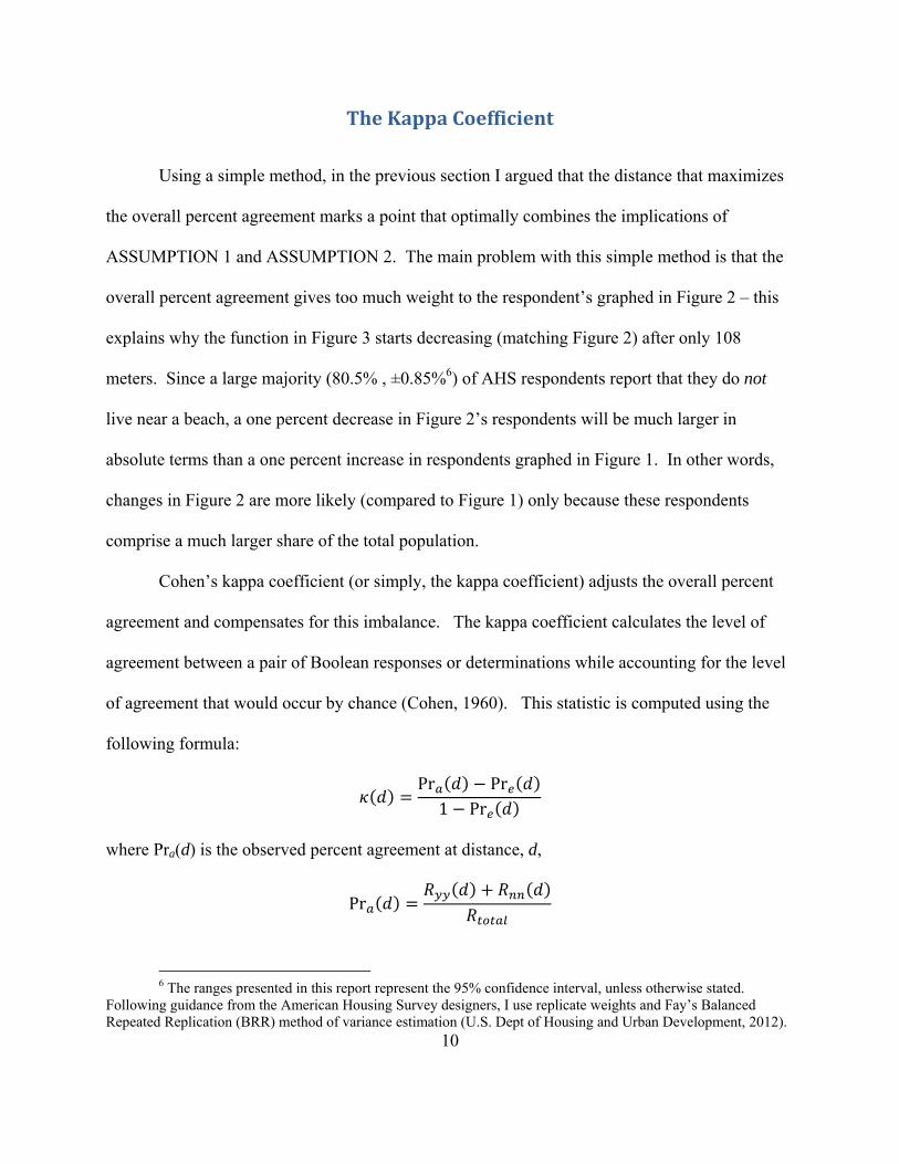
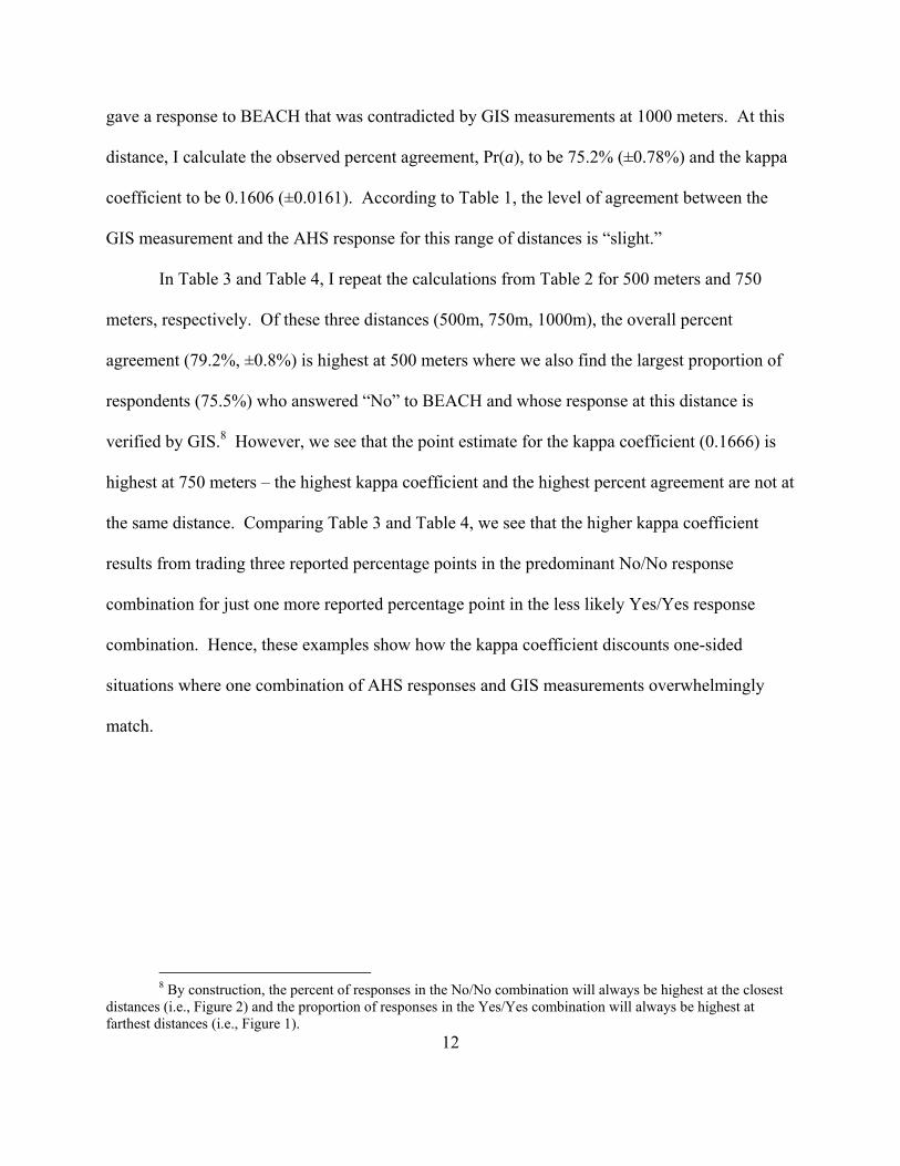
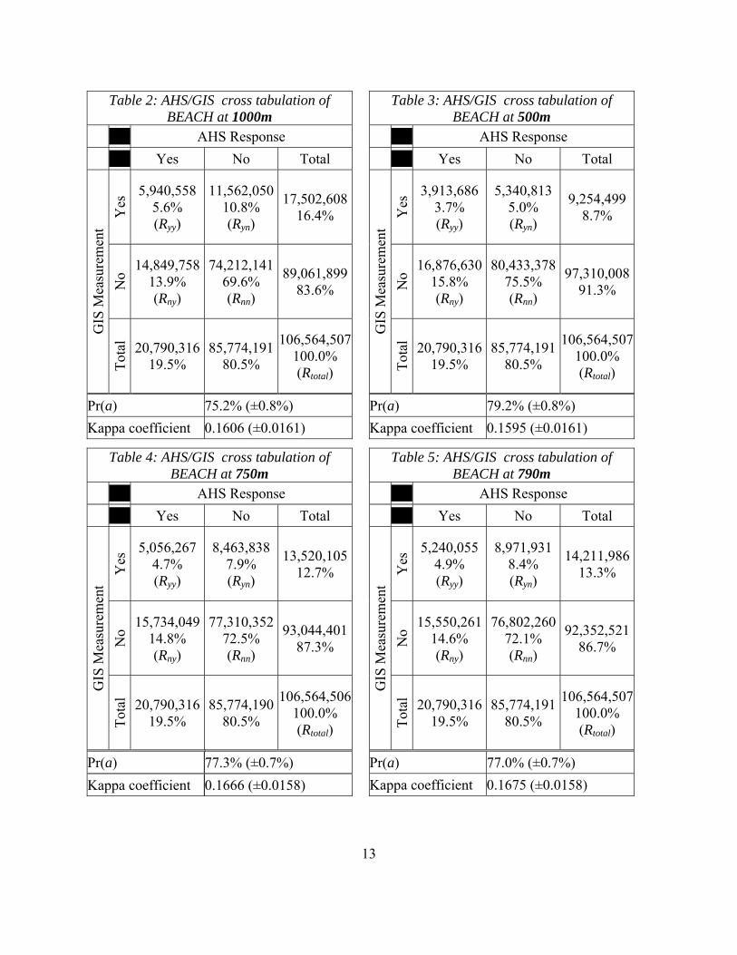
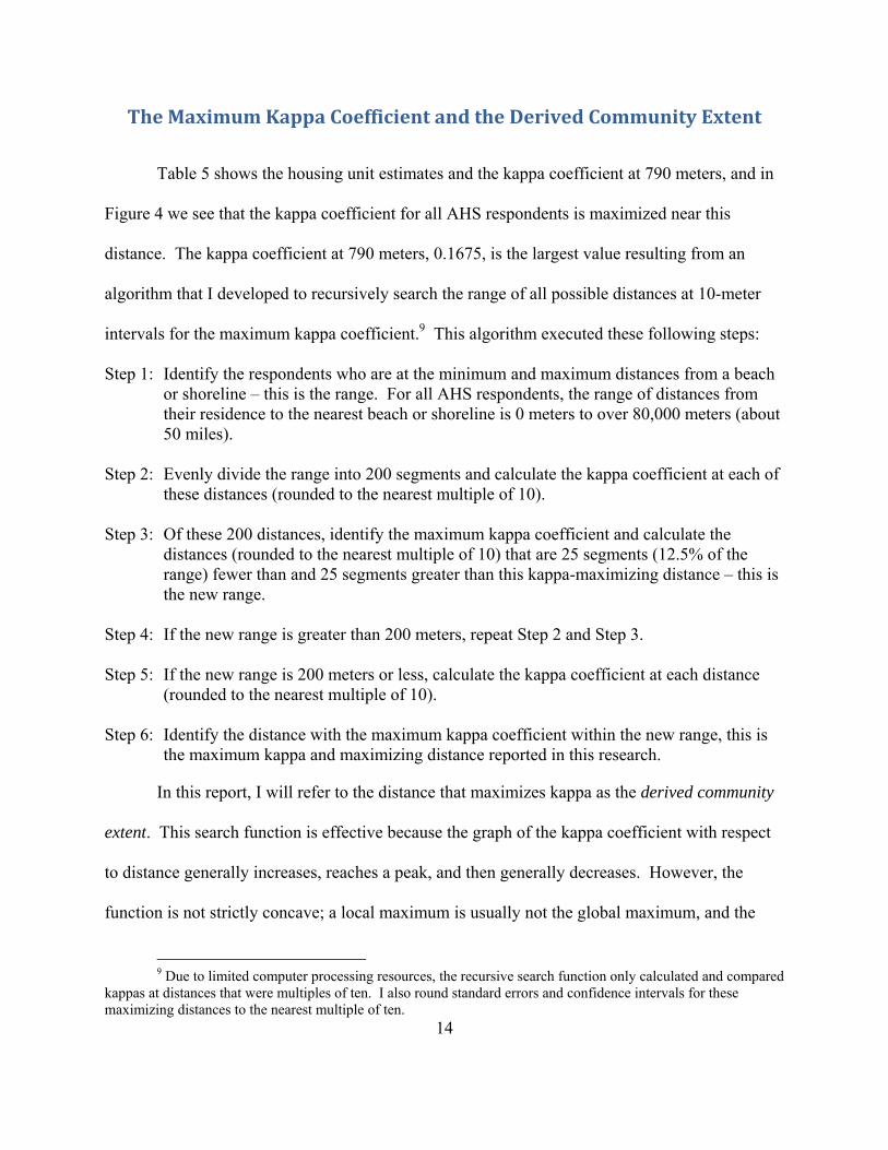
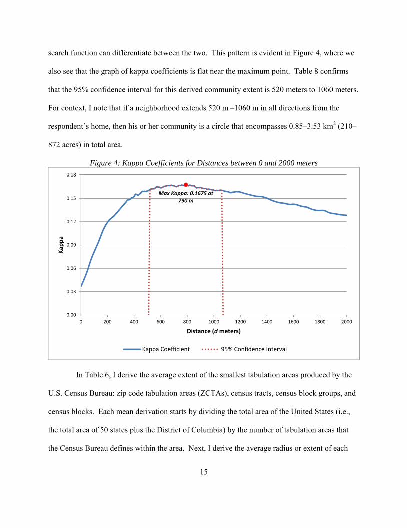
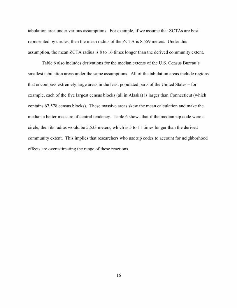
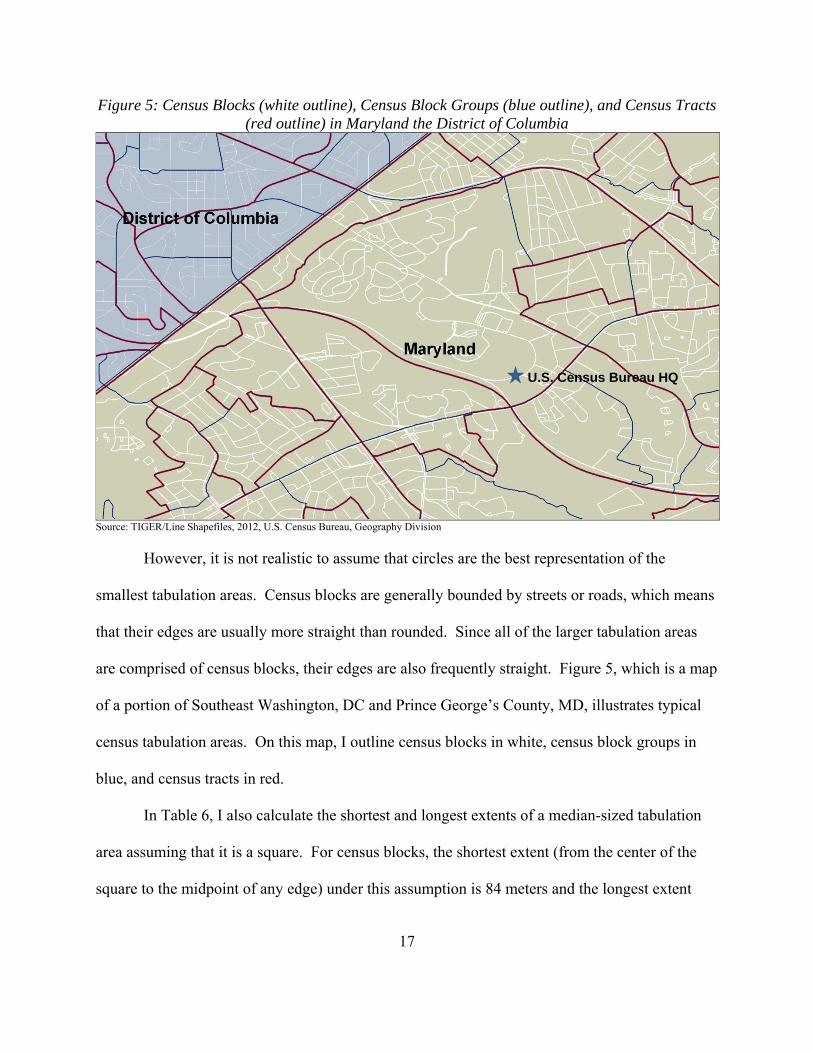
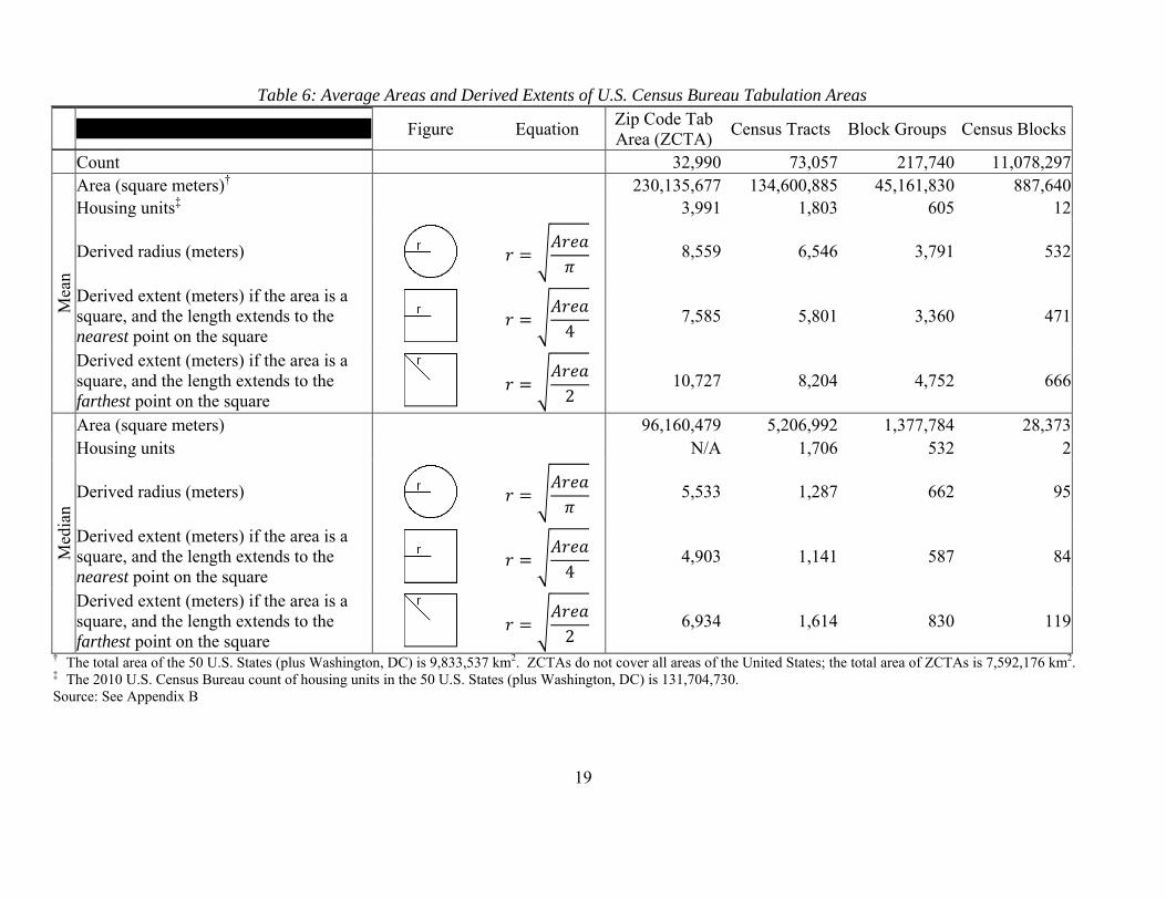
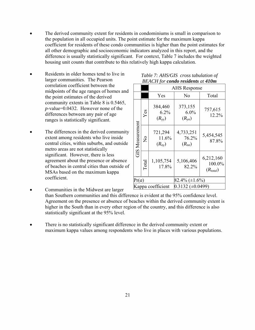
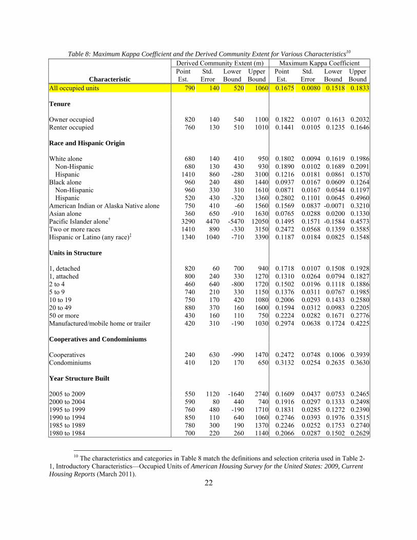
Table 8 Maximum Kappa Coefficient and the Derived Community Extent for Various Characteristics10
Characteristic
Derived Community Extent (m) Maximum Kappa Coefficient Point Est
Std Error
Lower Bound
Upper Bound
Point Est
Std Error
Lower Bound
Upper Bound
All occupied units
Tenure
790 140 520 1060 01675 00080 01518 01833
Owner occupied 820 140 540 1100 01822 00107 01613 02032 Renter occupied
Race and Hispanic Origin
760 130 510 1010 01441 00105 01235 01646
White alone 680 140 410 950 01802 00094 01619 01986 Non-Hispanic 680 130 430 930 01890 00102 01689 02091 Hispanic 1410 860 -280 3100 01216 00181 00861 01570
Black alone 960 240 480 1440 00937 00167 00609 01264 Non-Hispanic 960 330 310 1610 00871 00167 00544 01197 Hispanic 520 430 -320 1360 02802 01101 00645 04960
American Indian or Alaska Native alone 750 410 -60 1560 01569 00837 -00071 03210 Asian alone 360 650 -910 1630 00765 00288 00200 01330 Pacific Islander alonedagger 3290 4470 -5470 12050 01495 01571 -01584 04573 Two or more races 1410 890 -330 3150 02472 00568 01359 03585 Hispanic or Latino (any race)Dagger
Units in Structure
1340 1040 -710 3390 01187 00184 00825 01548
1 detached 820 60 700 940 01718 00107 01508 01928 1 attached 800 240 330 1270 01310 00264 00794 01827 2 to 4 460 640 -800 1720 01502 00196 01118 01886 5 to 9 740 210 330 1150 01376 00311 00767 01985 10 to 19 750 170 420 1080 02006 00293 01433 02580 20 to 49 880 370 160 1600 01594 00312 00983 02205 50 or more 430 160 110 750 02224 00282 01671 02776 Manufacturedmobile home or trailer
Cooperatives and Condominiums
420 310 -190 1030 02974 00638 01724 04225
Cooperatives 240 630 -990 1470 02472 00748 01006 03939 Condominiums
Year Structure Built
410 120 170 650 03132 00254 02635 03630
2005 to 2009 550 1120 -1640 2740 01609 00437 00753 02465 2000 to 2004 590 80 440 740 01916 00297 01333 02498 1995 to 1999 760 480 -190 1710 01831 00285 01272 02390 1990 to 1994 850 110 640 1060 02746 00393 01976 03515 1985 to 1989 780 300 190 1370 02246 00252 01753 02740 1980 to 1984 700 220 260 1140 02066 00287 01502 02629
10 The characteristics and categories in Table 8 match the definitions and selection criteria used in Table 2shy1 Introductory CharacteristicsmdashOccupied Units of American Housing Survey for the United States 2009 Current Housing Reports (March 2011)
22
Table 8 Maximum Kappa Coefficient and the Derived Community Extent for Various Characteristics10
Characteristic
Derived Community Extent (m) Maximum Kappa Coefficient Point Est
Std Error
Lower Bound
Upper Bound
Point Est
Std Error
Lower Bound
Upper Bound
1975 to 1979 550 190 180 920 01705 00228 01258 02152 1970 to 1974 780 220 360 1200 02124 00223 01688 02561 1960 to 1969 1180 710 -220 2580 01491 00170 01158 01824 1950 to 1959 850 640 -390 2090 01307 00176 00962 01651 1940 to 1949 1070 280 510 1630 01432 00235 00971 01893 1930 to 1939 710 150 410 1010 01418 00266 00896 01940 1920 to 1929 1430 1100 -720 3580 01030 00259 00522 01538 1919 or earlier
MetropolitanNonmetropolitan Areas
770 280 210 1330 01604 00225 01163 02044
Inside metropolitan statistical areas 800 110 580 1020 01557 00075 01410 01704 In central cities 790 180 430 1150 01276 00108 01064 01488 Suburbs 640 220 200 1080 01725 00100 01528 01922
Outside metropolitan statistical areas
Regions
750 210 330 1170 02221 00300 01634 02808
Northeast 680 190 300 1060 01501 00136 01235 01767 Midwest 1350 300 750 1950 01488 00180 01136 01840 South 500 80 340 660 02312 00194 01931 02692 West
Place Size
790 90 610 970 01427 00225 00986 01868
Fewer than 2500 persons 860 330 220 1500 01888 00392 01120 02656 2500 to 9999 persons 840 180 480 1200 01514 00205 01112 01917 10000 to 19999 persons 1400 950 -450 3250 01031 00231 00578 01483 20000 to 49999 persons 680 200 280 1080 01225 00164 00903 01547 50000 to 99999 persons 740 330 100 1380 01264 00190 00892 01635 100000 to 249999 persons 790 310 190 1390 01695 00251 01202 02188 250000 to 499999 persons 500 400 -290 1290 00604 00214 00185 01023 500000 to 999999 persons 1190 20 1160 1220 01669 00328 01026 02311 1000000 persons or more 430 1080 -1690 2550 01043 00185 00681 01405 dagger Native Hawaiian and Other Pacific Islander Dagger Because Hispanics may be any race data can overlap slightly with other groups Most Hispanics report
themselves as White but some report themselves as Black or in other categories
23
An Alternative Method for Deriving Neighborhood Size
In previous sections of this report I derived the community extent by comparing the
incidence of AHS respondents who report that a beach or shoreline is in their neighborhood with
the GIS-measured distance to the nearest body of water I defined this derived community extent
as the distance at which the level of agreement (measured by the kappa coefficient) between the
AHS response and the GIS measurement is maximized However this distance is difficult to
interpret For example it is convenient to assume that the derived community extent is the same
distance in every direction from the respondent but this implies that each neighborhood is circle
with its center at the respondentrsquos home Alternatively for the sake of analytical ease we might
imagine that each neighborhood is a square and the derived community extent measures the
distance to the nearest or farthest points of the square but this assumption also fails to capture
the unlimited variety of neighborhood shapes and sizes
In reality no community in America is a perfectly symmetric shape with a smooth
boundary centered on an AHS respondent Actual communities are usually simple polygons
with borders formed by well-established often-winding landmarks like highways rivers and
streams political jurisdictions etc Not incidentally the US Census Bureau uses many of these
same boundaries to help mark the edges of census blocks block groups tracts and ZCTAs11
This makes these tabulation areas ideal proxies for actual neighborhoods In this section I will
derive an estimate of community size that takes advantage of the potential alignment between
actual neighborhoods and tabulation areas
11 In the hierarchy of physical features that the US Census Bureau uses to create the boundaries of census blocks the highest priority shapes are (in order) water areas named and unnamed roads and political jurisdictions (US Census Bureau 1994)
24
Similar to the approach that I described in the previous sections (which I will refer to as
Method A) I will compare the incidence of AHS respondents who report that a beach or
shoreline is in their community with the GIS-determined presence or absence of a significant
body of water within census tabulation areas Then I will identify the tabulation areas (grouped
by size) that maximize the level of agreement (measured by kappa) between the AHS response
and the GIS observation I will call this second approach Method B12
As an example see Figure 6 which is a map identifying census blocks (white outline)
block groups (blue outline) and tracts (red outline) in Miami Beach FL For the sake of this
example I have pinpointed two
hypothetical AHS respondents Imagine
that Respondent A answered ldquoYesrdquo to
BEACH Since neither her census block
nor block group border the ocean these
tabulation areas obviously cannot outline
the area that she would say is in her
community ndash I assume that these areas are
too small If her neighborhood is
coextensive with a census tabulation area
then it must match either her census tract or
ZCTA (none of Miami Beachrsquos five zip
codes is landlocked)
Figure 6 Census Blocks (white outline) Census Block Groups (blue outline) and Census Tracts
(red outline) in Miami Beach FL
Source TIGERLine Shapefiles 2012 US Census Bureau Note I chose the location of Respondent A and Respondent B for the purpose of this illustration These locations may or may not pinpoint the addresses of actual AHS respondents
12 I acknowledge and thank Charles A Bee my colleague at the US Census Bureau for proposing Method B
25
Alternatively consider Respondent B who answered ldquoNordquo to BEACH Since this
respondentrsquos block group tract and ZCTA border the ocean I conclude that these tabulation
areas are too big to match this respondentrsquos conception of his community If a tabulation area
happens to be coterminous with this respondentrsquos community then it must be his census block13
When creating tabulation areas the US Census Bureau respects many of the same natural and
political boundaries that outline actual communities which means that a tabulation area might
share the same physical space as real neighborhoods and subdivisions However this will only
be true for AHS survey respondents when their answer to BEACH agrees with the GIS-
determined presence or absence of a body of water in the tabulation area My objective in
Method B is to identify the size of tabulation areas that maximizes the level of agreement
between the AHS response and the GIS determination
Table 9 details the results of this analysis which proceeded along these steps
Step 1 Locate every AHS respondent who answered BEACH within his or her census block block group tract and ZCTA and create an expanded AHS sample that includes duplicate entries for each of these four tabulation areas
Step 2 Sort this expanded sample by the size of the tabulation area and divide this dataset into 120 classes having roughly the same weighted number of housing units (not the unweighted number of cases) For the sample of all occupied housing units I find that the average area of the smallest class is approximately equal to the playing surface of an American football field and the average area in the largest class is larger than the cities of Los Angeles and Chicago combined The median-sized class is the same size as New York Cityrsquos Central Park
Not surprisingly the smallest classes are entirely composed of census blocks and the largest classes are dominated by ZCTAs The derived radius in Table 9 is the distance from the center of the average area to its edge assuming that its shape is a circle
ݒݎ ݏݑݎ ඥൌݎݒ ݎߨ
13 Method B separately considers four tabulation areas (blocks block groups tracts and ZCTAs) as potential neighborhoods that align with the respondentrsquos own community therefore this analysis counts each interview as many as four times
26
Step 3 Determine the AHS ResponseGIS Determination combination of weighted household counts within each class Notice the pattern of disagreement between the AHS Response and the GIS Determination in Table 9 Where there is disagreement in the smallest areas it is overwhelmingly because the AHS respondent gave an affirmative answer to BEACH but GIS determined that the tabulation area does not contain a large body of water Disagreement in the largest areas is primarily due to the AHS respondent giving a negative response to BEACH where GIS determined that there is a body of water within the tabulation area
Step 4 Calculate the percent agreement and the kappa coefficient for each class and identify the maximum kappa coefficient For the sample of all occupied housing units the kappa coefficient is maximized in the 58th class The average size for the 58th class is comparable in area to the primary airport in Baton Rouge LA (BTR) Buffalo NY (BUF) or Santa Barbara CA (SBA) The derived radius for this class (987 meters) implies that these tabulation areas fit within the 95 confidence interval of the derived community extent that I calculated earlier in this report using Method A (between 520 and 1060 meters)
27
5
10
15
20
25
30
35
40
45
50
55
60
65
Table 9 Selected Statistics by Class Using Method B for All Occupied Housing Units
Class Housing Units Average Area
(m2) Derived
Radius (m) Blocks Block
Groups Tracts ZCTAs AHS ResponseGIS Determination Percent
Agree Kappa Coeff
Smooth KappaYesYes NoYes YesNo NoNo
1 3549533 5142 40 100 0 0 0 17531 28741 926405 2576856 731 00108 2 3552921 8884 53 100 0 0 0 11407 15341 837083 2689089 760 00116 3 3547052 11272 60 100 0 0 0 33968 16693 721923 2774468 792 00590 00252 4 3554486 13436 65 100 0 0 0 21007 21252 841768 2670459 757 00243 00285
3552276 15586 70 99 1 0 0 17672 21038 815607 2697959 764 00201 00304 6 3551547 17589 75 98 2 0 0 15950 11616 718263 2805718 794 00273 00333 7 3550045 19612 79 99 1 0 0 16315 19363 766038 2748329 779 00211 00345 8 3553198 21544 83 98 2 0 0 41929 14723 731182 2765364 790 00735 00455 9 3551292 24046 87 97 3 0 0 29528 36287 831413 2654064 756 00303 00435
3551485 27157 93 98 2 0 0 37560 14082 659439 2840404 810 00753 00439 11 3551209 30675 99 96 4 0 0 18891 35111 766231 2730976 774 00171 00307 12 3550409 34775 105 95 5 0 0 18599 31324 689407 2811079 797 00234 00349 13 3550923 39351 112 94 6 0 0 16088 41411 783533 2709892 768 00076 00366 14 3550922 44748 119 93 7 0 0 30454 33622 644825 2842020 809 00511 00536
3550699 52126 129 91 9 0 0 48949 28066 691714 2781970 797 00837 00791 16 3552516 61140 140 89 11 0 0 59117 62104 588006 2843289 817 01023 00957 17 3552379 71907 151 86 12 1 0 75792 17079 628388 2831121 818 01510 01146 18 3551247 85378 165 85 14 1 0 52883 62181 584993 2851190 818 00905 01233 19 3549964 101944 180 80 18 2 0 71998 57558 529224 2891184 835 01457 01308
3552434 121817 197 73 23 4 0 77653 45872 666561 2762349 799 01269 01200 21 3550452 144179 214 67 24 10 0 77543 66316 567192 2839400 822 01397 01210 22 3553450 166163 230 53 29 18 0 67841 76925 643539 2765145 797 00974 01078 23 3550113 189155 245 57 29 14 0 63528 98745 563156 2824683 814 00954 01127 24 3551664 217505 263 53 36 10 0 60019 82909 647486 2761250 794 00795 01110
3550524 248991 282 47 44 8 0 117107 118275 635508 2679633 788 01513 00998 26 3552455 281947 300 47 46 8 0 90338 127464 549571 2785082 809 01312 00987 27 3549955 316794 318 36 54 10 0 43759 95979 654810 2755406 789 00415 01117 28 3553038 349773 334 39 53 9 0 73295 99854 659947 2719941 786 00900 00964 29 3546341 387887 351 33 55 12 0 93550 89616 596179 2766996 807 01445 00920
3556304 430156 370 35 54 11 0 70813 133104 627222 2725165 786 00749 01099 31 3549869 474275 389 27 61 12 0 99758 138400 660180 2651531 775 01089 01101 32 3552438 518186 406 28 60 11 0 129595 191990 623341 2607512 770 01310 01032 33 3552694 566885 425 25 60 15 0 85801 144968 634297 2687628 781 00910 01061 34 3551071 616740 443 24 61 14 0 86335 129423 596068 2739245 796 01101 01058
3550959 658236 458 18 65 17 0 66314 121490 557958 2805198 809 00893 01172 36 3551307 705964 474 23 60 16 2 106511 183441 611045 2650310 776 01077 01229 37 3552382 765617 494 25 60 15 0 165369 169155 620527 2597331 778 01879 01177 38 3549990 827769 513 22 59 18 1 118613 220636 564617 2646125 779 01196 01177 39 3552614 894129 533 23 54 23 1 95995 239569 540449 2676601 780 00842 01177
3551623 965993 555 22 52 25 1 106703 242612 573207 2629101 770 00890 01031 41 3548641 1036220 574 20 52 25 2 106262 251395 498179 2692804 789 01079 01150 42 3553031 1116167 596 18 52 29 1 120296 256503 531943 2644289 778 01148 01160 43 3550334 1200484 618 19 49 31 1 160240 259821 496580 2633693 787 01791 01128 44 3552157 1279055 638 14 43 43 1 78997 184194 520645 2768321 802 00893 01158
3552325 1346817 655 18 45 37 1 98402 257313 561683 2634927 769 00731 01118 46 3551123 1437011 676 16 47 35 2 140243 317102 503020 2590759 769 01228 01135 47 3550151 1543722 701 15 40 42 3 119429 284901 546865 2598957 766 00948 01103 48 3552934 1655841 726 18 39 41 3 193835 354638 456246 2548216 772 01874 01270 49 3551655 1769588 751 15 42 41 2 135489 375139 551269 2489758 739 00735 01101
3551252 1892028 776 14 36 45 4 163310 283308 532765 2571870 770 01566 01210 51 3551782 2016421 801 13 36 49 2 83678 289215 553738 2625152 763 00382 01074 52 3550971 2158234 829 15 35 47 3 197042 389242 514983 2449704 745 01495 01072 53 3550921 2294293 855 14 36 46 4 182061 443957 491019 2433884 737 01194 01017 54 3550634 2444877 882 13 34 50 3 136112 364328 570258 2479936 737 00725 01160
3552465 2578116 906 13 26 58 3 110243 207500 519975 2714747 795 01290 01053 56 3549962 2691009 926 12 29 55 5 162622 401394 508137 2477809 744 01097 01254 57 3552802 2862014 954 13 30 45 11 174894 499843 474628 2403438 726 00957 01339 58 3551623 3063461 987 11 33 53 3 259892 448828 425184 2417718 754 02199 01330 59 3551447 3292028 1024 10 32 51 7 176091 492980 436931 2445446 738 01153 01207
3550938 3527420 1060 12 27 54 7 214756 507186 492713 2336283 718 01242 01255 61 3551724 3772725 1096 9 27 54 9 172397 536531 552427 2290369 693 00484 01247 62 3550978 4032666 1133 13 26 48 13 203856 578949 414166 2354006 720 01198 01328 63 3551809 4350033 1177 6 28 58 8 266187 498220 398058 2389345 748 02157 01432 64 3550740 4683853 1221 8 29 52 11 284377 673330 402344 2190688 697 01557 01688
3552374 5060758 1269 10 27 53 10 244656 467135 473685 2366898 735 01764 01788 66 3549533 5418256 1313 10 25 52 14 286381 605347 417333 2240472 712 01765 01659
28
Table 9 Selected Statistics by Class Using Method B for All Occupied Housing Units
Class Housing Units Average Area
(m2) Derived
Radius (m) Blocks Block
Groups Tracts ZCTAs AHS ResponseGIS Determination Percent
Agree Kappa Coeff
Smooth KappaYesYes NoYes YesNo NoNo
67 3552450 5829364 1362 8 28 46 18 330254 729755 392401 2100040 684 01696 01563 68 3550654 6307479 1417 9 27 45 20 298971 733850 386079 2131755 685 01511 01522 69 3552106 6836571 1475 7 26 45 23 331254 823568 450434 1946850 641 01080 01400 70 3550649 7428593 1538 5 28 46 21 334822 772439 393342 2050045 672 01560 01230 71 3552884 8022909 1598 6 27 43 24 307469 805794 419158 2020463 655 01153 01061 72 3550282 8746589 1669 5 24 39 33 276615 847487 412779 2013401 645 00847 01104 73 3552476 9521904 1741 4 28 35 32 288356 884485 442074 1937561 627 00664 00949 74 3550191 10335667 1814 4 26 40 30 326236 821400 401035 2001520 656 01298 01045 75 3552858 11246662 1892 4 25 37 34 273267 849737 420544 2009310 642 00783 01177 76 3551343 12258202 1975 2 26 33 39 425518 832735 428230 1864860 645 01633 01277 77 3550172 13267068 2055 2 22 34 43 387269 916748 358601 1887554 641 01509 01250 78 3550416 14341750 2137 4 19 32 45 356377 950065 375368 1868605 627 01162 01309 79 3553358 15433165 2216 3 21 30 47 334677 827519 434636 1956526 645 01163 01202 80 3551771 16553973 2295 1 19 27 53 297469 872296 376629 2005377 648 01078 01241 81 3551324 17685221 2373 1 22 24 53 393163 953544 420005 1784611 613 01099 01039 82 3548644 18882424 2452 1 19 24 56 456600 1023338 309802 1758905 624 01705 00997 83 3553685 20165250 2534 1 19 26 55 286909 1056413 442251 1768113 578 00148 01089 84 3550143 21682064 2627 1 20 22 57 437643 1246848 311765 1553887 561 00953 01115 85 3552462 23304432 2724 1 18 22 59 404554 987477 323458 1836973 631 01540 00993 86 3550183 24994782 2821 1 19 27 52 350843 1019879 315348 1864112 624 01230 01155 87 3552672 26941195 2928 1 20 20 60 364671 1143301 287129 1757570 597 01096 01093 88 3551524 28958104 3036 1 20 22 57 346307 1167215 286078 1751924 591 00956 01026 89 3551884 31071411 3145 2 23 20 55 398039 1239941 346940 1566964 553 00643 00817 90 3551569 33455115 3263 0 18 23 59 445577 1189596 300389 1616006 580 01206 00890 91 3550935 35996274 3385 0 20 21 59 316312 1420421 297528 1516674 516 00184 00834 92 3548854 38862404 3517 0 24 21 55 451228 1174938 264959 1657728 594 01460 00901 93 3554147 42281507 3669 0 18 20 61 438036 1445165 270709 1400238 517 00679 00885 94 3551464 46127146 3832 0 20 26 54 430780 1469658 204898 1446127 528 00977 01079 95 3551126 49796707 3981 0 22 25 53 510877 1482977 208485 1348786 524 01123 00989 96 3550691 54034258 4147 0 21 22 57 426235 1350567 220503 1553386 558 01155 01089 97 3552568 58703124 4323 0 19 24 57 376788 1509698 155945 1510138 531 01013 01042 98 3548662 63743436 4504 0 20 23 56 472273 1448430 197442 1430518 536 01177 01059 99 3553592 69209181 4694 0 19 25 56 437596 1574915 208560 1332520 498 00744 01045
100 3551945 75521187 4903 0 17 22 60 447788 1509094 157397 1437665 531 01207 00940 101 3550885 82706555 5131 0 15 26 59 498599 1550150 183015 1319122 512 01084 00767 102 3549164 89896798 5349 0 18 27 55 395309 1744193 178600 1231061 458 00488 00830 103 3552572 98293652 5594 0 19 30 51 417768 1628509 255052 1251244 470 00311 00740 104 3551369 108566221 5879 0 17 22 61 403581 1559348 143529 1444911 521 01062 00703 105 3551784 118958192 6154 0 16 29 56 418806 1573908 198392 1360677 501 00757 00768 106 3550025 130175425 6437 0 13 19 67 512183 1875600 104195 1058048 442 00897 00858 107 3552656 143724330 6764 0 9 27 64 402556 1476498 217264 1456339 523 00811 00797 108 3551029 158891060 7112 0 14 24 62 476122 1683637 180310 1210960 475 00762 00839 109 3552285 177878083 7525 0 8 29 63 415489 1736032 143513 1257251 471 00757 00825 110 3550482 195015323 7879 0 12 23 66 501089 1474112 235222 1340059 519 00967 00772 111 3552926 216936651 8310 0 6 25 69 492306 1829413 126387 1104820 450 00826 00741 112 3550120 244642836 8825 0 9 31 60 426550 1836280 152559 1134731 440 00546 00581 113 3552101 277539297 9399 0 4 26 69 515254 2049019 102051 885778 394 00608 00562 114 3551401 311686969 9961 0 5 27 68 421994 2285270 138406 705731 318 -00043 00366 115 3551820 351316076 10575 0 4 27 69 447909 1733050 136002 1234859 474 00873 00512 116 3550224 397550515 11249 0 5 18 76 479499 2017298 226149 827278 368 -00152 00356 117 3552767 458675178 12083 0 5 28 67 493939 1607957 127214 1323657 512 01272 00250 118 3549890 562730050 13384 0 6 29 65 477492 2113850 202977 755571 347 -00169 -00214 119 3551233 793477243 15893 0 5 26 69 443966 2446500 189440 471327 258 -00574 120 3553188 2217410809 26567 0 9 39 52 517930 2200827 371238 463192 276 -01446
I have highlighted the 58th class where the kappa coefficient is maximized
29
Figure 7 Kappa Coefficients Using Method B
03 Kap
pa
02
01
00
‐01
‐02
Max Kappa 02199 at 1064862 m2
Size (m2) of Tabulation Area
Kappa Coeff Smooth Kappa 95 Confidence Interval
Figure 7 illustrates the data that I have calculated in Table 9 In this figure I plot kappa
coefficients on the vertical axis and the average size of the tabulation area in square meters on
the horizontal axis Notice that the horizontal axis is a logarithmic (base 10) scale ndash each tick
mark indicates an average area that is ten times larger than the previous tick mark The blue
points plotted in Figure 7 are the kappa coefficients calculated in Table 9 The red ldquosmooth
kappardquo line traces a rolling average of five kappa coefficients
where i is a class number between 3 and ሻାଶhellip ଶሺൌ ݐݏ
118 This smooth kappa line illustrates a clear pattern ndash the kappa coefficients for the smallest
and largest tabulation areas are generally low and the peak kappa coefficients occur in midshy
range tabulation areas I will refer to the class of tabulation areas where kappa is maximized as
the derived community area Using replicate weights I find that the 95 confidence interval for
30
the derived community area of all occupied housing units using Method B is 370399 m2 to
25339614 m2 I indicate this confidence internal by the shaded region of Figure 7 If these
upper and lower threshold areas were circles then the derived radius for this range would be 343
m to 2840 m which fully overlaps the derived community extent that I previously calculated
using Method A (520 m ndash 1060 m)
I repeat Method B for the same demographic and socioeconomic groups that I analyzed
using Method A in Table 8 and I present these findings in Table 10 Comparing the two tables I
find no statistically significant differences between any of the derived community extents (of
Method A) and the derived community areas (of Method B) This conclusion assumes that the
shape of the derived community area is a circle and the derived radius measures the distance
from the AHS respondentrsquos home to the edge of his or her community Under this assumption
there is no subpopulation analyzed in Table 8Table 10 in which the confidence intervals do not
overlap at the standard levels for statistical significance
Additionally the confidence intervals using Method B are wider than the confidence
intervals using Method A for all 50 of the subpopulations analyzed in Table 8Table 10 In 35
out of the 50 subpopulations the 95 confidence interval that I derived using Method B
completely overlaps (ie has a smaller lower bound and a larger upper bound than) the 95
confidence interval using Method A Based on these observations I conclude that Method A
produces more precise estimates of community size than Method B
31
Table 10 Alternate Maximum Kappa Coefficient and the Derived Community Area for Various Characteristics14
Characteristic
Derived Community Area (m2) Maximum Kappa Coefficient Point
Est Std
Error Lower Bound
Upper Bound
Point Est
Std Error
Lower Bound
Upper Bound
All occupied units
Tenure
Owner occupied Renter occupied
Race and Hispanic Origin
White alone Non-Hispanic Hispanic Black alone Non-Hispanic HispanicAmerican Indian or Alaska Native alone Asian alone Pacific Islander alonedagger
Two or more races Hispanic or Latino (any race)Dagger
Units in Structure
1 detached 1 attached 2 to 4 5 to 9 10 to 19 20 to 49 50 or more Manufacturedmobile home or trailer
Cooperatives and Condominiums
Cooperatives Condominiums
Year Structure Built
2005 to 2009 2000 to 2004 1995 to 1999 1990 to 1994 1985 to 1989 1980 to 1984
64862 04682 55686 74038
66402 08580 49586 83218 64826 11143 42987 86665
66866 10974 45358 88374 62098 08608 45226 78971 67342 09721 48288 86395 58067 18100 22591 93542 60826 11314 38650 83002
ndash ndash ndash ndash ndash ndash ndash ndash
62825 10546 42156 83495 ndash ndash ndash ndash ndash ndash ndash ndash
56016 18792 19185 92847
66446 08278 50222 82669 59507 07854 44114 74901 58835 08562 42055 75616 70896 19744 32198 109594 56009 09683 37030 74987 63451 14238 35545 91357 51190 10379 30847 71533 63190 14964 33861 92519
ndash ndash ndash ndash 54258 13559 27682 80834
67932 13098 42260 93603 66104 20588 25751 106456 60937 12626 36190 85684 48626 42065 -33820 131072 64832 25503 14846 114818 65294 09198 47266 83323
02199 00312 01588 02810
02483 00399 01701 03265 02630 00567 01519 03741
02287 00325 01651 02923 02331 00397 01552 03109 04153 01103 01992 06315 03404 00849 01741 05068 03308 01041 01268 05348
ndash ndash ndash ndash ndash ndash ndash ndash
03043 03276 -03378 09464 ndash ndash ndash ndash ndash ndash ndash ndash
03645 00823 02031 05259
02054 00555 00968 03141 04550 01495 01619 07481 04907 01405 02152 07661 02848 03769 -04539 10235 05911 02782 00459 11364 05777 01687 02471 09083 05484 02060 01446 09522 05525 03272 -00888 11937
ndash ndash ndash ndash 05039 02248 00632 09445
05023 02063 00979 09066 05741 02453 00934 10549 04064 01271 01573 06556 04878 04062 -03083 12840 04491 01341 01863 07119 04827 01181 02511 07142
14 The characteristics and categories in Table 10 match the definitions and selection criteria used in Table 2-1 Introductory CharacteristicsmdashOccupied Units of American Housing Survey for the United States 2009 Current Housing Reports (March 2011)
32
Table 10 Alternate Maximum Kappa Coefficient and the Derived Community Area for Various Characteristics14
Characteristic
Derived Community Area (m2) Maximum Kappa Coefficient Point
Est Std
Error Lower Bound
Upper Bound
Point Est
Std Error
Lower Bound
Upper Bound
1975 to 1979 63205 08916 45731 80680 04281 01041 02241 06321 1970 to 1974 55742 11198 33794 77691 04098 01583 00996 07200 1960 to 1969 65422 11855 42185 88658 02971 01169 00679 05262 1950 to 1959 74249 12899 48967 99532 02929 01339 00305 05553 1940 to 1949 66651 07442 52065 81237 04216 01377 01518 06914 1930 to 1939 58271 15374 28138 88405 03685 01759 00238 07132 1920 to 1929 64974 14892 35786 94163 03965 01557 00914 07016 1919 or earlier
MetropolitanNonmetropolitan Areas
78253 22802 33562 122944 03994 00932 02166 05821
Inside metropolitan statistical areas 66451 06940 52849 80053 02048 00426 01213 02882 In central cities 62655 12177 38788 86521 02820 00559 01724 03916 Suburbs 70855 09679 51885 89826 02244 00737 00800 03687 Outside metropolitan statistical areas
Regions
86575 40248 07691 165459 04266 01191 01932 06599
Northeast 60771 08861 43404 78137 03029 00746 01567 04492 Midwest 86661 16266 54781 118542 04125 01633 00925 07326 South 49010 16947 15795 82225 03569 00754 02090 05047 West
Place Size
68835 09764 49697 87973 02945 00801 01374 04515
Fewer than 2500 persons 67795 12458 43378 92211 04591 03092 -01470 10651 2500 to 9999 persons 59092 12781 34041 84143 03869 01079 01753 05984 10000 to 19999 persons 62127 14298 34104 90151 03171 01544 00145 06196 20000 to 49999 persons 67935 06988 54238 81631 02716 01427 -00080 05513 50000 to 99999 persons 60836 12473 36390 85282 04407 01342 01776 07037 100000 to 249999 persons 63832 07711 48718 78947 04689 00964 02800 06578 250000 to 499999 persons 62902 16201 31148 94656 03194 01811 -00355 06742 500000 to 999999 persons 72784 17094 39280 106288 05890 01607 02741 09039 1000000 persons or more 71135 27236 17754 124516 03939 01631 00742 07136 Derived Community Area (m2) is the value of the exponent with a base of 10 (eg 64862 = 1064862 = 3063374) dagger Native Hawaiian and Other Pacific Islander Dagger Because Hispanics may be any race data can overlap slightly with other groups Most Hispanics report
themselves as White but some report themselves as Black or in other categories ndash Indicates a characteristic with too few cases (30 or fewer) to produce useful statistical inferences
33
Conclusion
In this report I used data from the 2009 American Housing Survey in conjunction with
various GIS maps and tools to determine that the distance from the typical Americanrsquos house to
the edge of his community is between 520 and 1060 meters This derived community extent is
roughly equal to the radius of one or two median-sized census block groups Not surprisingly
condo communities and communities with 50 or more housing units per building are smaller than
communities of typical single family (detached) homes I also found a regional variation in
community size communities in the Midwest are larger than those in the South These findings
are not contradicted by an alternative method of deriving neighborhood size that accounts for
variations in the neighborhoodrsquos shape
34
References
Carroll T Clauretie T amp Neill H (1997) Effect of Foreclosure Status on Residential Selling
Price Comment Journal of Real Estate Research 13(1) 95-102
Cohen J (1960) A Coefficient of Agreement for Nominal Scales Educational and
Psychological Measurement XX(1) 37-46
Forgey F A Ronald R C amp VanBuskirk M L (1994) Effect of foreclosure status on
residential selling price Journal of Real Estate Research 9(3) 313ndash18
Frame W (2010) Estimating the Effect of Mortgage Foreclosures on Estimating the Effect of
Mortgage Foreclosures on Federal Reserve Bank of Atlanta Economic Review 95(3) 1shy
9
Immergluck D amp Smith G (2005) Measuring the effects of subprime lending on
neighborhood foreclosures Evidence from Chicago Urban Affairs Review 40 362ndash389
Immergluck D amp Smith G (2006 November) The Impact of Single-family Mortgage
Foreclosures on Neighborhood Crime Housing Studies 21(6) 851ndash866
Immergluck D amp Smith G (2006b) The External Costs of Foreclosure The Impact of Single-
Family Mortgage Foreclosures on Property Values Housing Policy Debate 17 57ndash79
Landis J R amp Koch G G (1977 March) The Measurement of Observer Agreement for
Categorical Data Biometrics 33(1) 159-174
Lin Z Rosenblatt E amp Yao V (2009) Spillover effects of foreclosures on neighborhood
property values Journal of Real Estate Finance and Economics 38(4) 387ndash407
Schuetz J Been V amp Ellen I G (2008) Neighborhood Effects of Concentrated Mortgage
Foreclosures Journal of Housing Economics 17 306ndash319
35
Taylor R B (2012) Defining Neighborhoods in Space and Time Cityscape A Journal of
Policy Development and Research 225-230
US Census Bureau (2011) Guide to State and Local Census Geography 2011 Retrieved
November 27 2012 from US Census Bureau
httpwwwcensusgovgeowwwguidestlocpdfAll_GSLCGpdf
US Census Bureau (2011) Current Housing Reports Series H15009 American Housing
Survey for the United States 2009 Washington DC 20401 US Government Printing
Office
US Dept of Housing and Urban Development (2012 November 14) Estimating AHS National
Variances with Replicate Weights Retrieved November 27 2012 from HUD USER
httpwwwhuduserorgportaldatasetsahsAHSN_Public_Use_Replicate_Weight_abbre
viated31OCT12pdf
36
Appendix A The Neighborhood Quality Section of the 2009 AHS
GATED The following questions are about your community Is your community surrounded by walls or fences preventing access by persons other than residents
1 Yes 2 No
GATEDV The following questions are about your community (Last time) we recorded that your community is surrounded by walls or fences preventing access by persons other than residents Is this information still correct
1 Yes 2 No
ACCESSC Does access to your community require a special entry system such as entry codes key cards or security guard approval
1 Yes 2 No
ACCESSCV (Last time) we recorded access to your community requires a special entry system such as entry codes key cards or security guard approval Is this information still correct
1 Yes 2 No
ACCESSB Does access to your building require a special entry system such as entry codes key cards or security guard approval
1 Yes 2 No
ACCESSBV (Last time) we recorded access to your building requires a special entry system such as entry codes key cards or security guard approval Is this information still correct
1 Yes 2 No
37
AGERES You mentioned that one or more members of your household are 55 or older Some communities are age-restricted meaning that at least one member of the family must be at least 55 years or older Is your development age-restricted
1 Yes 2 No
AGERESV (Last time) we recorded that your development was age-restricted meaning that at least one member of the family must be at least 55 years or older Is this information still correct
1 Yes 2 No
NORC Sometimes communities that are not age-restricted still attract certain age groups Do you believe the majority of your neighbors are 55 or over
1 Yes 2 No
CLUB Are any of the following features included in your community Community Center or Clubhouse
1 Yes 2 No
GOLF (Are any of the following features included in your community) Golf Course
1 Yes 2 No
TRAILS (Are any of the following features included in your community) WalkingJogging Trails
1 Yes 2 No
SHUTLE (Are any of the following features included in your community) Shuttle Bus
1 Yes 2 No
38
CARE (Are any of the following features included in your community) Day Care Center
1 Yes 2 No
BEACH (Are any of the following features included in your community) Beach Park or Shoreline
1 Yes 2 No
39
Appendix B Selected Statistics and Tabulation Area Counts by State
State Area (m2) Counts
Housing Units ZCTAs Census Tracts Block Groups Census Blocks Alabama 135767342446 2171853 629 1181 3438 252266 Alaska 1723336523156 306967 238 167 534 45292 Arizona 295232869248 2844526 362 1526 4178 241666 Arkansas 137731828968 1316299 504 686 2147 186211 California 423966968085 13680081 1719 8057 23212 710145 Colorado 269603398884 2212898 525 1249 3532 201062 Connecticut 14357375332 1487891 391 833 2585 67578 Delaware 6445769842 405885 67 218 574 24115 District of Columbia 176999744 296719 53 179 450 6507 Florida 170311608772 8989580 1028 4245 11442 484481 Georgia 153910578723 4088801 695 1969 5533 291086 Hawaii 28312992182 519508 95 351 875 25016 Idaho 216443477713 667796 206 298 963 149842 Illinois 149995304656 5296715 1381 3123 9691 451554 Indiana 94326221957 2795541 731 1511 4814 267071 Iowa 145745891267 1336417 684 825 2630 216007 Kansas 213099965684 1233215 561 770 2351 238600 Kentucky 104655683036 1927164 605 1115 3285 161672 Louisiana 135656018836 1964981 571 1148 3471 204447 Maine 91634122036 721830 432 358 1086 69518 Maryland 32131089610 2378814 491 1406 3926 145247 Massachusetts 27335741928 2808254 331 1478 4985 157508 Michigan 250486780758 4532233 987 2813 8205 329885 Minnesota 225161404423 2347201 798 1338 4111 259777 Mississippi 125455713880 1274719 382 664 2164 171778 Missouri 180540279352 2712729 1231 1393 4506 343565 Montana 380832074499 482825 361 271 842 132288 Nebraska 200328701612 796793 654 532 1633 193352 Nevada 286380145586 1173814 242 687 1836 84538 New Hampshire 24214215247 614754 194 295 922 48837 New Jersey 22591379380 3553562 595 2010 6320 169588 New Mexico 314917547864 901388 309 499 1449 168609 New York 141296785159 8108103 1793 4919 15464 350169 North Carolina 139390789884 4327528 833 2195 6155 288987 North Dakota 183107810720 317498 526 205 572 133769 Ohio 116097706996 5127508 1224 2952 9238 365344 Oklahoma 181037235141 1664378 633 1046 2965 269118 Oregon 254799589926 1675562 458 834 2634 196621 Pennsylvania 119280059748 5567315 1853 3218 9740 421545 Rhode Island 4001234100 463388 175 244 815 25181 South Carolina 82932660230 2137683 363 1103 3059 181908 South Dakota 199728851315 363438 443 222 654 88360 Tennessee 109153130302 2812133 811 1497 4125 240116 Texas 695661526826 9977436 2012 5265 15811 914231 Utah 219884162541 979709 288 588 1690 115406 Vermont 24906267580 322539 309 184 522 32580 Virginia 110786551025 3364939 826 1907 5332 285762 Washington 184661284315 2885677 630 1458 4783 195574 West Virginia 62756019147 881917 835 484 1592 135218 Wisconsin 169634848618 2624358 749 1409 4489 253096 Wyoming 253334294812 261868 177 132 410 86204 Totaldagger 9833536823091 131704730 32990 73057 217740 11078297
dagger ZCTAs do not cover all areas of the United States the total area of ZCTAs is 7592175985321 m2 Source TIGERLine Shapefiles 2012 US Census Bureau Geography Division
40
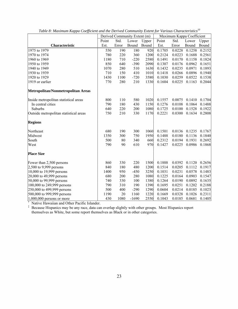
Table 8 Maximum Kappa Coefficient and the Derived Community Extent for Various Characteristics10
Characteristic
Derived Community Extent (m) Maximum Kappa Coefficient Point Est
Std Error
Lower Bound
Upper Bound
Point Est
Std Error
Lower Bound
Upper Bound
1975 to 1979 550 190 180 920 01705 00228 01258 02152 1970 to 1974 780 220 360 1200 02124 00223 01688 02561 1960 to 1969 1180 710 -220 2580 01491 00170 01158 01824 1950 to 1959 850 640 -390 2090 01307 00176 00962 01651 1940 to 1949 1070 280 510 1630 01432 00235 00971 01893 1930 to 1939 710 150 410 1010 01418 00266 00896 01940 1920 to 1929 1430 1100 -720 3580 01030 00259 00522 01538 1919 or earlier
MetropolitanNonmetropolitan Areas
770 280 210 1330 01604 00225 01163 02044
Inside metropolitan statistical areas 800 110 580 1020 01557 00075 01410 01704 In central cities 790 180 430 1150 01276 00108 01064 01488 Suburbs 640 220 200 1080 01725 00100 01528 01922
Outside metropolitan statistical areas
Regions
750 210 330 1170 02221 00300 01634 02808
Northeast 680 190 300 1060 01501 00136 01235 01767 Midwest 1350 300 750 1950 01488 00180 01136 01840 South 500 80 340 660 02312 00194 01931 02692 West
Place Size
790 90 610 970 01427 00225 00986 01868
Fewer than 2500 persons 860 330 220 1500 01888 00392 01120 02656 2500 to 9999 persons 840 180 480 1200 01514 00205 01112 01917 10000 to 19999 persons 1400 950 -450 3250 01031 00231 00578 01483 20000 to 49999 persons 680 200 280 1080 01225 00164 00903 01547 50000 to 99999 persons 740 330 100 1380 01264 00190 00892 01635 100000 to 249999 persons 790 310 190 1390 01695 00251 01202 02188 250000 to 499999 persons 500 400 -290 1290 00604 00214 00185 01023 500000 to 999999 persons 1190 20 1160 1220 01669 00328 01026 02311 1000000 persons or more 430 1080 -1690 2550 01043 00185 00681 01405 dagger Native Hawaiian and Other Pacific Islander Dagger Because Hispanics may be any race data can overlap slightly with other groups Most Hispanics report
themselves as White but some report themselves as Black or in other categories
23
An Alternative Method for Deriving Neighborhood Size
In previous sections of this report I derived the community extent by comparing the
incidence of AHS respondents who report that a beach or shoreline is in their neighborhood with
the GIS-measured distance to the nearest body of water I defined this derived community extent
as the distance at which the level of agreement (measured by the kappa coefficient) between the
AHS response and the GIS measurement is maximized However this distance is difficult to
interpret For example it is convenient to assume that the derived community extent is the same
distance in every direction from the respondent but this implies that each neighborhood is circle
with its center at the respondentrsquos home Alternatively for the sake of analytical ease we might
imagine that each neighborhood is a square and the derived community extent measures the
distance to the nearest or farthest points of the square but this assumption also fails to capture
the unlimited variety of neighborhood shapes and sizes
In reality no community in America is a perfectly symmetric shape with a smooth
boundary centered on an AHS respondent Actual communities are usually simple polygons
with borders formed by well-established often-winding landmarks like highways rivers and
streams political jurisdictions etc Not incidentally the US Census Bureau uses many of these
same boundaries to help mark the edges of census blocks block groups tracts and ZCTAs11
This makes these tabulation areas ideal proxies for actual neighborhoods In this section I will
derive an estimate of community size that takes advantage of the potential alignment between
actual neighborhoods and tabulation areas
11 In the hierarchy of physical features that the US Census Bureau uses to create the boundaries of census blocks the highest priority shapes are (in order) water areas named and unnamed roads and political jurisdictions (US Census Bureau 1994)
24
Similar to the approach that I described in the previous sections (which I will refer to as
Method A) I will compare the incidence of AHS respondents who report that a beach or
shoreline is in their community with the GIS-determined presence or absence of a significant
body of water within census tabulation areas Then I will identify the tabulation areas (grouped
by size) that maximize the level of agreement (measured by kappa) between the AHS response
and the GIS observation I will call this second approach Method B12
As an example see Figure 6 which is a map identifying census blocks (white outline)
block groups (blue outline) and tracts (red outline) in Miami Beach FL For the sake of this
example I have pinpointed two
hypothetical AHS respondents Imagine
that Respondent A answered ldquoYesrdquo to
BEACH Since neither her census block
nor block group border the ocean these
tabulation areas obviously cannot outline
the area that she would say is in her
community ndash I assume that these areas are
too small If her neighborhood is
coextensive with a census tabulation area
then it must match either her census tract or
ZCTA (none of Miami Beachrsquos five zip
codes is landlocked)
Figure 6 Census Blocks (white outline) Census Block Groups (blue outline) and Census Tracts
(red outline) in Miami Beach FL
Source TIGERLine Shapefiles 2012 US Census Bureau Note I chose the location of Respondent A and Respondent B for the purpose of this illustration These locations may or may not pinpoint the addresses of actual AHS respondents
12 I acknowledge and thank Charles A Bee my colleague at the US Census Bureau for proposing Method B
25
Alternatively consider Respondent B who answered ldquoNordquo to BEACH Since this
respondentrsquos block group tract and ZCTA border the ocean I conclude that these tabulation
areas are too big to match this respondentrsquos conception of his community If a tabulation area
happens to be coterminous with this respondentrsquos community then it must be his census block13
When creating tabulation areas the US Census Bureau respects many of the same natural and
political boundaries that outline actual communities which means that a tabulation area might
share the same physical space as real neighborhoods and subdivisions However this will only
be true for AHS survey respondents when their answer to BEACH agrees with the GIS-
determined presence or absence of a body of water in the tabulation area My objective in
Method B is to identify the size of tabulation areas that maximizes the level of agreement
between the AHS response and the GIS determination
Table 9 details the results of this analysis which proceeded along these steps
Step 1 Locate every AHS respondent who answered BEACH within his or her census block block group tract and ZCTA and create an expanded AHS sample that includes duplicate entries for each of these four tabulation areas
Step 2 Sort this expanded sample by the size of the tabulation area and divide this dataset into 120 classes having roughly the same weighted number of housing units (not the unweighted number of cases) For the sample of all occupied housing units I find that the average area of the smallest class is approximately equal to the playing surface of an American football field and the average area in the largest class is larger than the cities of Los Angeles and Chicago combined The median-sized class is the same size as New York Cityrsquos Central Park
Not surprisingly the smallest classes are entirely composed of census blocks and the largest classes are dominated by ZCTAs The derived radius in Table 9 is the distance from the center of the average area to its edge assuming that its shape is a circle
ݒݎ ݏݑݎ ඥൌݎݒ ݎߨ
13 Method B separately considers four tabulation areas (blocks block groups tracts and ZCTAs) as potential neighborhoods that align with the respondentrsquos own community therefore this analysis counts each interview as many as four times
26
Step 3 Determine the AHS ResponseGIS Determination combination of weighted household counts within each class Notice the pattern of disagreement between the AHS Response and the GIS Determination in Table 9 Where there is disagreement in the smallest areas it is overwhelmingly because the AHS respondent gave an affirmative answer to BEACH but GIS determined that the tabulation area does not contain a large body of water Disagreement in the largest areas is primarily due to the AHS respondent giving a negative response to BEACH where GIS determined that there is a body of water within the tabulation area
Step 4 Calculate the percent agreement and the kappa coefficient for each class and identify the maximum kappa coefficient For the sample of all occupied housing units the kappa coefficient is maximized in the 58th class The average size for the 58th class is comparable in area to the primary airport in Baton Rouge LA (BTR) Buffalo NY (BUF) or Santa Barbara CA (SBA) The derived radius for this class (987 meters) implies that these tabulation areas fit within the 95 confidence interval of the derived community extent that I calculated earlier in this report using Method A (between 520 and 1060 meters)
27
5
10
15
20
25
30
35
40
45
50
55
60
65
Table 9 Selected Statistics by Class Using Method B for All Occupied Housing Units
Class Housing Units Average Area
(m2) Derived
Radius (m) Blocks Block
Groups Tracts ZCTAs AHS ResponseGIS Determination Percent
Agree Kappa Coeff
Smooth KappaYesYes NoYes YesNo NoNo
1 3549533 5142 40 100 0 0 0 17531 28741 926405 2576856 731 00108 2 3552921 8884 53 100 0 0 0 11407 15341 837083 2689089 760 00116 3 3547052 11272 60 100 0 0 0 33968 16693 721923 2774468 792 00590 00252 4 3554486 13436 65 100 0 0 0 21007 21252 841768 2670459 757 00243 00285
3552276 15586 70 99 1 0 0 17672 21038 815607 2697959 764 00201 00304 6 3551547 17589 75 98 2 0 0 15950 11616 718263 2805718 794 00273 00333 7 3550045 19612 79 99 1 0 0 16315 19363 766038 2748329 779 00211 00345 8 3553198 21544 83 98 2 0 0 41929 14723 731182 2765364 790 00735 00455 9 3551292 24046 87 97 3 0 0 29528 36287 831413 2654064 756 00303 00435
3551485 27157 93 98 2 0 0 37560 14082 659439 2840404 810 00753 00439 11 3551209 30675 99 96 4 0 0 18891 35111 766231 2730976 774 00171 00307 12 3550409 34775 105 95 5 0 0 18599 31324 689407 2811079 797 00234 00349 13 3550923 39351 112 94 6 0 0 16088 41411 783533 2709892 768 00076 00366 14 3550922 44748 119 93 7 0 0 30454 33622 644825 2842020 809 00511 00536
3550699 52126 129 91 9 0 0 48949 28066 691714 2781970 797 00837 00791 16 3552516 61140 140 89 11 0 0 59117 62104 588006 2843289 817 01023 00957 17 3552379 71907 151 86 12 1 0 75792 17079 628388 2831121 818 01510 01146 18 3551247 85378 165 85 14 1 0 52883 62181 584993 2851190 818 00905 01233 19 3549964 101944 180 80 18 2 0 71998 57558 529224 2891184 835 01457 01308
3552434 121817 197 73 23 4 0 77653 45872 666561 2762349 799 01269 01200 21 3550452 144179 214 67 24 10 0 77543 66316 567192 2839400 822 01397 01210 22 3553450 166163 230 53 29 18 0 67841 76925 643539 2765145 797 00974 01078 23 3550113 189155 245 57 29 14 0 63528 98745 563156 2824683 814 00954 01127 24 3551664 217505 263 53 36 10 0 60019 82909 647486 2761250 794 00795 01110
3550524 248991 282 47 44 8 0 117107 118275 635508 2679633 788 01513 00998 26 3552455 281947 300 47 46 8 0 90338 127464 549571 2785082 809 01312 00987 27 3549955 316794 318 36 54 10 0 43759 95979 654810 2755406 789 00415 01117 28 3553038 349773 334 39 53 9 0 73295 99854 659947 2719941 786 00900 00964 29 3546341 387887 351 33 55 12 0 93550 89616 596179 2766996 807 01445 00920
3556304 430156 370 35 54 11 0 70813 133104 627222 2725165 786 00749 01099 31 3549869 474275 389 27 61 12 0 99758 138400 660180 2651531 775 01089 01101 32 3552438 518186 406 28 60 11 0 129595 191990 623341 2607512 770 01310 01032 33 3552694 566885 425 25 60 15 0 85801 144968 634297 2687628 781 00910 01061 34 3551071 616740 443 24 61 14 0 86335 129423 596068 2739245 796 01101 01058
3550959 658236 458 18 65 17 0 66314 121490 557958 2805198 809 00893 01172 36 3551307 705964 474 23 60 16 2 106511 183441 611045 2650310 776 01077 01229 37 3552382 765617 494 25 60 15 0 165369 169155 620527 2597331 778 01879 01177 38 3549990 827769 513 22 59 18 1 118613 220636 564617 2646125 779 01196 01177 39 3552614 894129 533 23 54 23 1 95995 239569 540449 2676601 780 00842 01177
3551623 965993 555 22 52 25 1 106703 242612 573207 2629101 770 00890 01031 41 3548641 1036220 574 20 52 25 2 106262 251395 498179 2692804 789 01079 01150 42 3553031 1116167 596 18 52 29 1 120296 256503 531943 2644289 778 01148 01160 43 3550334 1200484 618 19 49 31 1 160240 259821 496580 2633693 787 01791 01128 44 3552157 1279055 638 14 43 43 1 78997 184194 520645 2768321 802 00893 01158
3552325 1346817 655 18 45 37 1 98402 257313 561683 2634927 769 00731 01118 46 3551123 1437011 676 16 47 35 2 140243 317102 503020 2590759 769 01228 01135 47 3550151 1543722 701 15 40 42 3 119429 284901 546865 2598957 766 00948 01103 48 3552934 1655841 726 18 39 41 3 193835 354638 456246 2548216 772 01874 01270 49 3551655 1769588 751 15 42 41 2 135489 375139 551269 2489758 739 00735 01101
3551252 1892028 776 14 36 45 4 163310 283308 532765 2571870 770 01566 01210 51 3551782 2016421 801 13 36 49 2 83678 289215 553738 2625152 763 00382 01074 52 3550971 2158234 829 15 35 47 3 197042 389242 514983 2449704 745 01495 01072 53 3550921 2294293 855 14 36 46 4 182061 443957 491019 2433884 737 01194 01017 54 3550634 2444877 882 13 34 50 3 136112 364328 570258 2479936 737 00725 01160
3552465 2578116 906 13 26 58 3 110243 207500 519975 2714747 795 01290 01053 56 3549962 2691009 926 12 29 55 5 162622 401394 508137 2477809 744 01097 01254 57 3552802 2862014 954 13 30 45 11 174894 499843 474628 2403438 726 00957 01339 58 3551623 3063461 987 11 33 53 3 259892 448828 425184 2417718 754 02199 01330 59 3551447 3292028 1024 10 32 51 7 176091 492980 436931 2445446 738 01153 01207
3550938 3527420 1060 12 27 54 7 214756 507186 492713 2336283 718 01242 01255 61 3551724 3772725 1096 9 27 54 9 172397 536531 552427 2290369 693 00484 01247 62 3550978 4032666 1133 13 26 48 13 203856 578949 414166 2354006 720 01198 01328 63 3551809 4350033 1177 6 28 58 8 266187 498220 398058 2389345 748 02157 01432 64 3550740 4683853 1221 8 29 52 11 284377 673330 402344 2190688 697 01557 01688
3552374 5060758 1269 10 27 53 10 244656 467135 473685 2366898 735 01764 01788 66 3549533 5418256 1313 10 25 52 14 286381 605347 417333 2240472 712 01765 01659
28
Table 9 Selected Statistics by Class Using Method B for All Occupied Housing Units
Class Housing Units Average Area
(m2) Derived
Radius (m) Blocks Block
Groups Tracts ZCTAs AHS ResponseGIS Determination Percent
Agree Kappa Coeff
Smooth KappaYesYes NoYes YesNo NoNo
67 3552450 5829364 1362 8 28 46 18 330254 729755 392401 2100040 684 01696 01563 68 3550654 6307479 1417 9 27 45 20 298971 733850 386079 2131755 685 01511 01522 69 3552106 6836571 1475 7 26 45 23 331254 823568 450434 1946850 641 01080 01400 70 3550649 7428593 1538 5 28 46 21 334822 772439 393342 2050045 672 01560 01230 71 3552884 8022909 1598 6 27 43 24 307469 805794 419158 2020463 655 01153 01061 72 3550282 8746589 1669 5 24 39 33 276615 847487 412779 2013401 645 00847 01104 73 3552476 9521904 1741 4 28 35 32 288356 884485 442074 1937561 627 00664 00949 74 3550191 10335667 1814 4 26 40 30 326236 821400 401035 2001520 656 01298 01045 75 3552858 11246662 1892 4 25 37 34 273267 849737 420544 2009310 642 00783 01177 76 3551343 12258202 1975 2 26 33 39 425518 832735 428230 1864860 645 01633 01277 77 3550172 13267068 2055 2 22 34 43 387269 916748 358601 1887554 641 01509 01250 78 3550416 14341750 2137 4 19 32 45 356377 950065 375368 1868605 627 01162 01309 79 3553358 15433165 2216 3 21 30 47 334677 827519 434636 1956526 645 01163 01202 80 3551771 16553973 2295 1 19 27 53 297469 872296 376629 2005377 648 01078 01241 81 3551324 17685221 2373 1 22 24 53 393163 953544 420005 1784611 613 01099 01039 82 3548644 18882424 2452 1 19 24 56 456600 1023338 309802 1758905 624 01705 00997 83 3553685 20165250 2534 1 19 26 55 286909 1056413 442251 1768113 578 00148 01089 84 3550143 21682064 2627 1 20 22 57 437643 1246848 311765 1553887 561 00953 01115 85 3552462 23304432 2724 1 18 22 59 404554 987477 323458 1836973 631 01540 00993 86 3550183 24994782 2821 1 19 27 52 350843 1019879 315348 1864112 624 01230 01155 87 3552672 26941195 2928 1 20 20 60 364671 1143301 287129 1757570 597 01096 01093 88 3551524 28958104 3036 1 20 22 57 346307 1167215 286078 1751924 591 00956 01026 89 3551884 31071411 3145 2 23 20 55 398039 1239941 346940 1566964 553 00643 00817 90 3551569 33455115 3263 0 18 23 59 445577 1189596 300389 1616006 580 01206 00890 91 3550935 35996274 3385 0 20 21 59 316312 1420421 297528 1516674 516 00184 00834 92 3548854 38862404 3517 0 24 21 55 451228 1174938 264959 1657728 594 01460 00901 93 3554147 42281507 3669 0 18 20 61 438036 1445165 270709 1400238 517 00679 00885 94 3551464 46127146 3832 0 20 26 54 430780 1469658 204898 1446127 528 00977 01079 95 3551126 49796707 3981 0 22 25 53 510877 1482977 208485 1348786 524 01123 00989 96 3550691 54034258 4147 0 21 22 57 426235 1350567 220503 1553386 558 01155 01089 97 3552568 58703124 4323 0 19 24 57 376788 1509698 155945 1510138 531 01013 01042 98 3548662 63743436 4504 0 20 23 56 472273 1448430 197442 1430518 536 01177 01059 99 3553592 69209181 4694 0 19 25 56 437596 1574915 208560 1332520 498 00744 01045
100 3551945 75521187 4903 0 17 22 60 447788 1509094 157397 1437665 531 01207 00940 101 3550885 82706555 5131 0 15 26 59 498599 1550150 183015 1319122 512 01084 00767 102 3549164 89896798 5349 0 18 27 55 395309 1744193 178600 1231061 458 00488 00830 103 3552572 98293652 5594 0 19 30 51 417768 1628509 255052 1251244 470 00311 00740 104 3551369 108566221 5879 0 17 22 61 403581 1559348 143529 1444911 521 01062 00703 105 3551784 118958192 6154 0 16 29 56 418806 1573908 198392 1360677 501 00757 00768 106 3550025 130175425 6437 0 13 19 67 512183 1875600 104195 1058048 442 00897 00858 107 3552656 143724330 6764 0 9 27 64 402556 1476498 217264 1456339 523 00811 00797 108 3551029 158891060 7112 0 14 24 62 476122 1683637 180310 1210960 475 00762 00839 109 3552285 177878083 7525 0 8 29 63 415489 1736032 143513 1257251 471 00757 00825 110 3550482 195015323 7879 0 12 23 66 501089 1474112 235222 1340059 519 00967 00772 111 3552926 216936651 8310 0 6 25 69 492306 1829413 126387 1104820 450 00826 00741 112 3550120 244642836 8825 0 9 31 60 426550 1836280 152559 1134731 440 00546 00581 113 3552101 277539297 9399 0 4 26 69 515254 2049019 102051 885778 394 00608 00562 114 3551401 311686969 9961 0 5 27 68 421994 2285270 138406 705731 318 -00043 00366 115 3551820 351316076 10575 0 4 27 69 447909 1733050 136002 1234859 474 00873 00512 116 3550224 397550515 11249 0 5 18 76 479499 2017298 226149 827278 368 -00152 00356 117 3552767 458675178 12083 0 5 28 67 493939 1607957 127214 1323657 512 01272 00250 118 3549890 562730050 13384 0 6 29 65 477492 2113850 202977 755571 347 -00169 -00214 119 3551233 793477243 15893 0 5 26 69 443966 2446500 189440 471327 258 -00574 120 3553188 2217410809 26567 0 9 39 52 517930 2200827 371238 463192 276 -01446
I have highlighted the 58th class where the kappa coefficient is maximized
29
Figure 7 Kappa Coefficients Using Method B
03 Kap
pa
02
01
00
‐01
‐02
Max Kappa 02199 at 1064862 m2
Size (m2) of Tabulation Area
Kappa Coeff Smooth Kappa 95 Confidence Interval
Figure 7 illustrates the data that I have calculated in Table 9 In this figure I plot kappa
coefficients on the vertical axis and the average size of the tabulation area in square meters on
the horizontal axis Notice that the horizontal axis is a logarithmic (base 10) scale ndash each tick
mark indicates an average area that is ten times larger than the previous tick mark The blue
points plotted in Figure 7 are the kappa coefficients calculated in Table 9 The red ldquosmooth
kappardquo line traces a rolling average of five kappa coefficients
where i is a class number between 3 and ሻାଶhellip ଶሺൌ ݐݏ
118 This smooth kappa line illustrates a clear pattern ndash the kappa coefficients for the smallest
and largest tabulation areas are generally low and the peak kappa coefficients occur in midshy
range tabulation areas I will refer to the class of tabulation areas where kappa is maximized as
the derived community area Using replicate weights I find that the 95 confidence interval for
30
the derived community area of all occupied housing units using Method B is 370399 m2 to
25339614 m2 I indicate this confidence internal by the shaded region of Figure 7 If these
upper and lower threshold areas were circles then the derived radius for this range would be 343
m to 2840 m which fully overlaps the derived community extent that I previously calculated
using Method A (520 m ndash 1060 m)
I repeat Method B for the same demographic and socioeconomic groups that I analyzed
using Method A in Table 8 and I present these findings in Table 10 Comparing the two tables I
find no statistically significant differences between any of the derived community extents (of
Method A) and the derived community areas (of Method B) This conclusion assumes that the
shape of the derived community area is a circle and the derived radius measures the distance
from the AHS respondentrsquos home to the edge of his or her community Under this assumption
there is no subpopulation analyzed in Table 8Table 10 in which the confidence intervals do not
overlap at the standard levels for statistical significance
Additionally the confidence intervals using Method B are wider than the confidence
intervals using Method A for all 50 of the subpopulations analyzed in Table 8Table 10 In 35
out of the 50 subpopulations the 95 confidence interval that I derived using Method B
completely overlaps (ie has a smaller lower bound and a larger upper bound than) the 95
confidence interval using Method A Based on these observations I conclude that Method A
produces more precise estimates of community size than Method B
31
Table 10 Alternate Maximum Kappa Coefficient and the Derived Community Area for Various Characteristics14
Characteristic
Derived Community Area (m2) Maximum Kappa Coefficient Point
Est Std
Error Lower Bound
Upper Bound
Point Est
Std Error
Lower Bound
Upper Bound
All occupied units
Tenure
Owner occupied Renter occupied
Race and Hispanic Origin
White alone Non-Hispanic Hispanic Black alone Non-Hispanic HispanicAmerican Indian or Alaska Native alone Asian alone Pacific Islander alonedagger
Two or more races Hispanic or Latino (any race)Dagger
Units in Structure
1 detached 1 attached 2 to 4 5 to 9 10 to 19 20 to 49 50 or more Manufacturedmobile home or trailer
Cooperatives and Condominiums
Cooperatives Condominiums
Year Structure Built
2005 to 2009 2000 to 2004 1995 to 1999 1990 to 1994 1985 to 1989 1980 to 1984
64862 04682 55686 74038
66402 08580 49586 83218 64826 11143 42987 86665
66866 10974 45358 88374 62098 08608 45226 78971 67342 09721 48288 86395 58067 18100 22591 93542 60826 11314 38650 83002
ndash ndash ndash ndash ndash ndash ndash ndash
62825 10546 42156 83495 ndash ndash ndash ndash ndash ndash ndash ndash
56016 18792 19185 92847
66446 08278 50222 82669 59507 07854 44114 74901 58835 08562 42055 75616 70896 19744 32198 109594 56009 09683 37030 74987 63451 14238 35545 91357 51190 10379 30847 71533 63190 14964 33861 92519
ndash ndash ndash ndash 54258 13559 27682 80834
67932 13098 42260 93603 66104 20588 25751 106456 60937 12626 36190 85684 48626 42065 -33820 131072 64832 25503 14846 114818 65294 09198 47266 83323
02199 00312 01588 02810
02483 00399 01701 03265 02630 00567 01519 03741
02287 00325 01651 02923 02331 00397 01552 03109 04153 01103 01992 06315 03404 00849 01741 05068 03308 01041 01268 05348
ndash ndash ndash ndash ndash ndash ndash ndash
03043 03276 -03378 09464 ndash ndash ndash ndash ndash ndash ndash ndash
03645 00823 02031 05259
02054 00555 00968 03141 04550 01495 01619 07481 04907 01405 02152 07661 02848 03769 -04539 10235 05911 02782 00459 11364 05777 01687 02471 09083 05484 02060 01446 09522 05525 03272 -00888 11937
ndash ndash ndash ndash 05039 02248 00632 09445
05023 02063 00979 09066 05741 02453 00934 10549 04064 01271 01573 06556 04878 04062 -03083 12840 04491 01341 01863 07119 04827 01181 02511 07142
14 The characteristics and categories in Table 10 match the definitions and selection criteria used in Table 2-1 Introductory CharacteristicsmdashOccupied Units of American Housing Survey for the United States 2009 Current Housing Reports (March 2011)
32
Table 10 Alternate Maximum Kappa Coefficient and the Derived Community Area for Various Characteristics14
Characteristic
Derived Community Area (m2) Maximum Kappa Coefficient Point
Est Std
Error Lower Bound
Upper Bound
Point Est
Std Error
Lower Bound
Upper Bound
1975 to 1979 63205 08916 45731 80680 04281 01041 02241 06321 1970 to 1974 55742 11198 33794 77691 04098 01583 00996 07200 1960 to 1969 65422 11855 42185 88658 02971 01169 00679 05262 1950 to 1959 74249 12899 48967 99532 02929 01339 00305 05553 1940 to 1949 66651 07442 52065 81237 04216 01377 01518 06914 1930 to 1939 58271 15374 28138 88405 03685 01759 00238 07132 1920 to 1929 64974 14892 35786 94163 03965 01557 00914 07016 1919 or earlier
MetropolitanNonmetropolitan Areas
78253 22802 33562 122944 03994 00932 02166 05821
Inside metropolitan statistical areas 66451 06940 52849 80053 02048 00426 01213 02882 In central cities 62655 12177 38788 86521 02820 00559 01724 03916 Suburbs 70855 09679 51885 89826 02244 00737 00800 03687 Outside metropolitan statistical areas
Regions
86575 40248 07691 165459 04266 01191 01932 06599
Northeast 60771 08861 43404 78137 03029 00746 01567 04492 Midwest 86661 16266 54781 118542 04125 01633 00925 07326 South 49010 16947 15795 82225 03569 00754 02090 05047 West
Place Size
68835 09764 49697 87973 02945 00801 01374 04515
Fewer than 2500 persons 67795 12458 43378 92211 04591 03092 -01470 10651 2500 to 9999 persons 59092 12781 34041 84143 03869 01079 01753 05984 10000 to 19999 persons 62127 14298 34104 90151 03171 01544 00145 06196 20000 to 49999 persons 67935 06988 54238 81631 02716 01427 -00080 05513 50000 to 99999 persons 60836 12473 36390 85282 04407 01342 01776 07037 100000 to 249999 persons 63832 07711 48718 78947 04689 00964 02800 06578 250000 to 499999 persons 62902 16201 31148 94656 03194 01811 -00355 06742 500000 to 999999 persons 72784 17094 39280 106288 05890 01607 02741 09039 1000000 persons or more 71135 27236 17754 124516 03939 01631 00742 07136 Derived Community Area (m2) is the value of the exponent with a base of 10 (eg 64862 = 1064862 = 3063374) dagger Native Hawaiian and Other Pacific Islander Dagger Because Hispanics may be any race data can overlap slightly with other groups Most Hispanics report
themselves as White but some report themselves as Black or in other categories ndash Indicates a characteristic with too few cases (30 or fewer) to produce useful statistical inferences
33
Conclusion
In this report I used data from the 2009 American Housing Survey in conjunction with
various GIS maps and tools to determine that the distance from the typical Americanrsquos house to
the edge of his community is between 520 and 1060 meters This derived community extent is
roughly equal to the radius of one or two median-sized census block groups Not surprisingly
condo communities and communities with 50 or more housing units per building are smaller than
communities of typical single family (detached) homes I also found a regional variation in
community size communities in the Midwest are larger than those in the South These findings
are not contradicted by an alternative method of deriving neighborhood size that accounts for
variations in the neighborhoodrsquos shape
34
References
Carroll T Clauretie T amp Neill H (1997) Effect of Foreclosure Status on Residential Selling
Price Comment Journal of Real Estate Research 13(1) 95-102
Cohen J (1960) A Coefficient of Agreement for Nominal Scales Educational and
Psychological Measurement XX(1) 37-46
Forgey F A Ronald R C amp VanBuskirk M L (1994) Effect of foreclosure status on
residential selling price Journal of Real Estate Research 9(3) 313ndash18
Frame W (2010) Estimating the Effect of Mortgage Foreclosures on Estimating the Effect of
Mortgage Foreclosures on Federal Reserve Bank of Atlanta Economic Review 95(3) 1shy
9
Immergluck D amp Smith G (2005) Measuring the effects of subprime lending on
neighborhood foreclosures Evidence from Chicago Urban Affairs Review 40 362ndash389
Immergluck D amp Smith G (2006 November) The Impact of Single-family Mortgage
Foreclosures on Neighborhood Crime Housing Studies 21(6) 851ndash866
Immergluck D amp Smith G (2006b) The External Costs of Foreclosure The Impact of Single-
Family Mortgage Foreclosures on Property Values Housing Policy Debate 17 57ndash79
Landis J R amp Koch G G (1977 March) The Measurement of Observer Agreement for
Categorical Data Biometrics 33(1) 159-174
Lin Z Rosenblatt E amp Yao V (2009) Spillover effects of foreclosures on neighborhood
property values Journal of Real Estate Finance and Economics 38(4) 387ndash407
Schuetz J Been V amp Ellen I G (2008) Neighborhood Effects of Concentrated Mortgage
Foreclosures Journal of Housing Economics 17 306ndash319
35
Taylor R B (2012) Defining Neighborhoods in Space and Time Cityscape A Journal of
Policy Development and Research 225-230
US Census Bureau (2011) Guide to State and Local Census Geography 2011 Retrieved
November 27 2012 from US Census Bureau
httpwwwcensusgovgeowwwguidestlocpdfAll_GSLCGpdf
US Census Bureau (2011) Current Housing Reports Series H15009 American Housing
Survey for the United States 2009 Washington DC 20401 US Government Printing
Office
US Dept of Housing and Urban Development (2012 November 14) Estimating AHS National
Variances with Replicate Weights Retrieved November 27 2012 from HUD USER
httpwwwhuduserorgportaldatasetsahsAHSN_Public_Use_Replicate_Weight_abbre
viated31OCT12pdf
36
Appendix A The Neighborhood Quality Section of the 2009 AHS
GATED The following questions are about your community Is your community surrounded by walls or fences preventing access by persons other than residents
1 Yes 2 No
GATEDV The following questions are about your community (Last time) we recorded that your community is surrounded by walls or fences preventing access by persons other than residents Is this information still correct
1 Yes 2 No
ACCESSC Does access to your community require a special entry system such as entry codes key cards or security guard approval
1 Yes 2 No
ACCESSCV (Last time) we recorded access to your community requires a special entry system such as entry codes key cards or security guard approval Is this information still correct
1 Yes 2 No
ACCESSB Does access to your building require a special entry system such as entry codes key cards or security guard approval
1 Yes 2 No
ACCESSBV (Last time) we recorded access to your building requires a special entry system such as entry codes key cards or security guard approval Is this information still correct
1 Yes 2 No
37
AGERES You mentioned that one or more members of your household are 55 or older Some communities are age-restricted meaning that at least one member of the family must be at least 55 years or older Is your development age-restricted
1 Yes 2 No
AGERESV (Last time) we recorded that your development was age-restricted meaning that at least one member of the family must be at least 55 years or older Is this information still correct
1 Yes 2 No
NORC Sometimes communities that are not age-restricted still attract certain age groups Do you believe the majority of your neighbors are 55 or over
1 Yes 2 No
CLUB Are any of the following features included in your community Community Center or Clubhouse
1 Yes 2 No
GOLF (Are any of the following features included in your community) Golf Course
1 Yes 2 No
TRAILS (Are any of the following features included in your community) WalkingJogging Trails
1 Yes 2 No
SHUTLE (Are any of the following features included in your community) Shuttle Bus
1 Yes 2 No
38
CARE (Are any of the following features included in your community) Day Care Center
1 Yes 2 No
BEACH (Are any of the following features included in your community) Beach Park or Shoreline
1 Yes 2 No
39
Appendix B Selected Statistics and Tabulation Area Counts by State
State Area (m2) Counts
Housing Units ZCTAs Census Tracts Block Groups Census Blocks Alabama 135767342446 2171853 629 1181 3438 252266 Alaska 1723336523156 306967 238 167 534 45292 Arizona 295232869248 2844526 362 1526 4178 241666 Arkansas 137731828968 1316299 504 686 2147 186211 California 423966968085 13680081 1719 8057 23212 710145 Colorado 269603398884 2212898 525 1249 3532 201062 Connecticut 14357375332 1487891 391 833 2585 67578 Delaware 6445769842 405885 67 218 574 24115 District of Columbia 176999744 296719 53 179 450 6507 Florida 170311608772 8989580 1028 4245 11442 484481 Georgia 153910578723 4088801 695 1969 5533 291086 Hawaii 28312992182 519508 95 351 875 25016 Idaho 216443477713 667796 206 298 963 149842 Illinois 149995304656 5296715 1381 3123 9691 451554 Indiana 94326221957 2795541 731 1511 4814 267071 Iowa 145745891267 1336417 684 825 2630 216007 Kansas 213099965684 1233215 561 770 2351 238600 Kentucky 104655683036 1927164 605 1115 3285 161672 Louisiana 135656018836 1964981 571 1148 3471 204447 Maine 91634122036 721830 432 358 1086 69518 Maryland 32131089610 2378814 491 1406 3926 145247 Massachusetts 27335741928 2808254 331 1478 4985 157508 Michigan 250486780758 4532233 987 2813 8205 329885 Minnesota 225161404423 2347201 798 1338 4111 259777 Mississippi 125455713880 1274719 382 664 2164 171778 Missouri 180540279352 2712729 1231 1393 4506 343565 Montana 380832074499 482825 361 271 842 132288 Nebraska 200328701612 796793 654 532 1633 193352 Nevada 286380145586 1173814 242 687 1836 84538 New Hampshire 24214215247 614754 194 295 922 48837 New Jersey 22591379380 3553562 595 2010 6320 169588 New Mexico 314917547864 901388 309 499 1449 168609 New York 141296785159 8108103 1793 4919 15464 350169 North Carolina 139390789884 4327528 833 2195 6155 288987 North Dakota 183107810720 317498 526 205 572 133769 Ohio 116097706996 5127508 1224 2952 9238 365344 Oklahoma 181037235141 1664378 633 1046 2965 269118 Oregon 254799589926 1675562 458 834 2634 196621 Pennsylvania 119280059748 5567315 1853 3218 9740 421545 Rhode Island 4001234100 463388 175 244 815 25181 South Carolina 82932660230 2137683 363 1103 3059 181908 South Dakota 199728851315 363438 443 222 654 88360 Tennessee 109153130302 2812133 811 1497 4125 240116 Texas 695661526826 9977436 2012 5265 15811 914231 Utah 219884162541 979709 288 588 1690 115406 Vermont 24906267580 322539 309 184 522 32580 Virginia 110786551025 3364939 826 1907 5332 285762 Washington 184661284315 2885677 630 1458 4783 195574 West Virginia 62756019147 881917 835 484 1592 135218 Wisconsin 169634848618 2624358 749 1409 4489 253096 Wyoming 253334294812 261868 177 132 410 86204 Totaldagger 9833536823091 131704730 32990 73057 217740 11078297
dagger ZCTAs do not cover all areas of the United States the total area of ZCTAs is 7592175985321 m2 Source TIGERLine Shapefiles 2012 US Census Bureau Geography Division
40
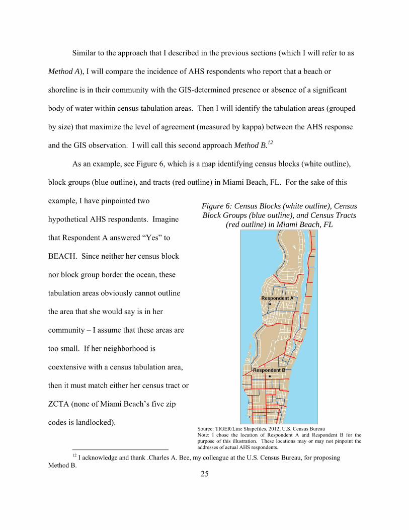
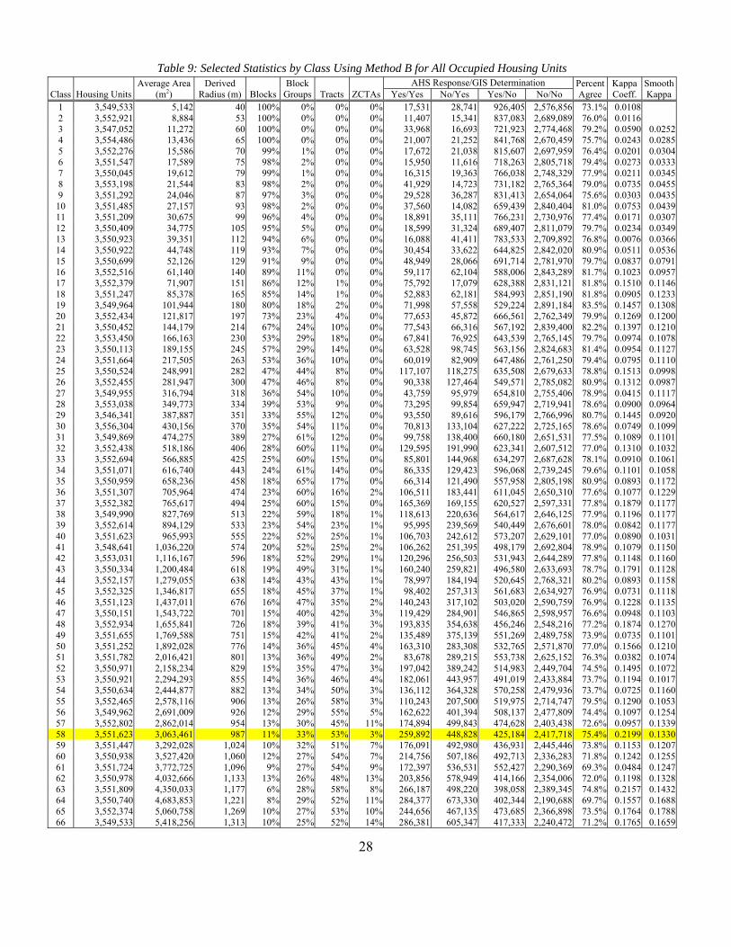
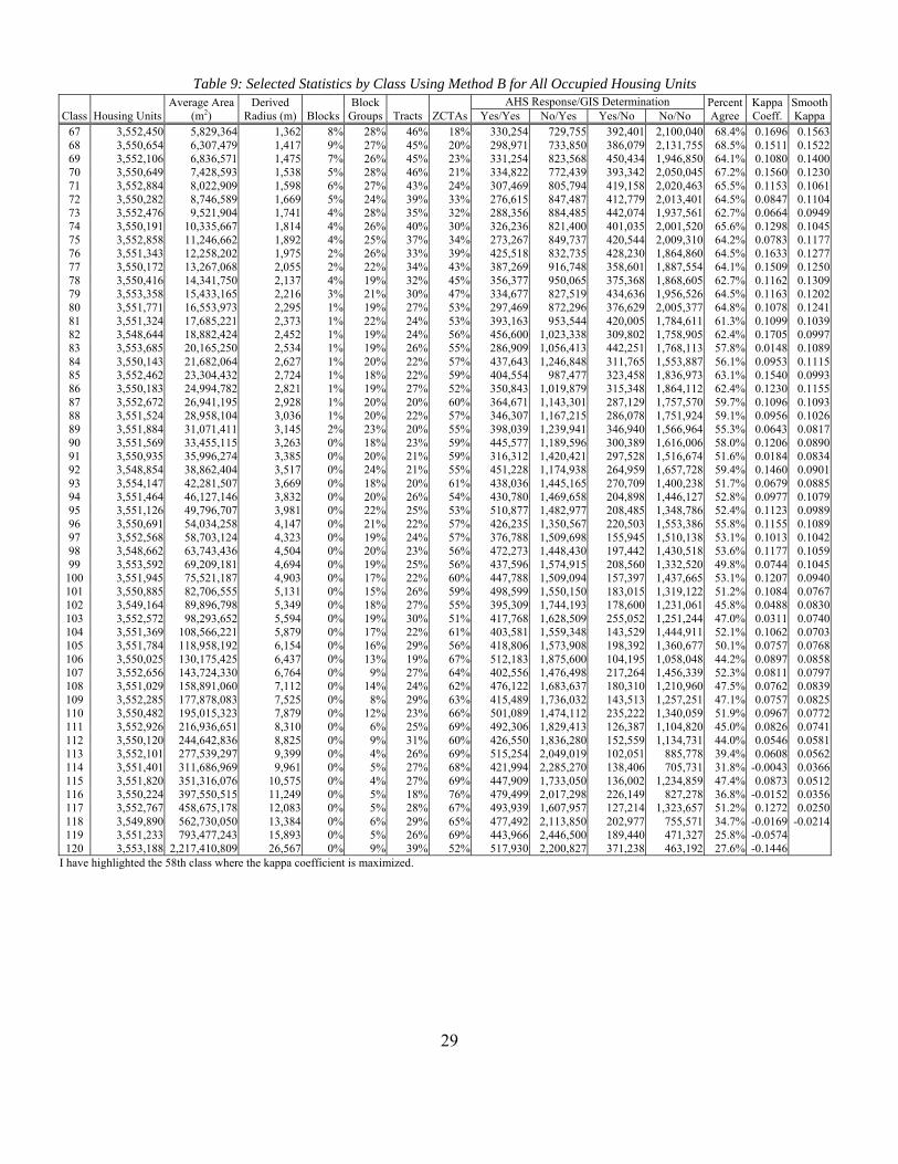
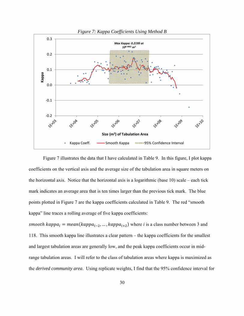
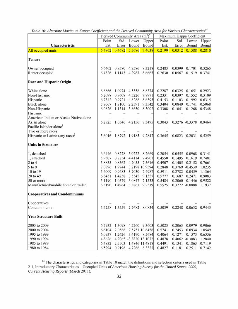
Table 10 Alternate Maximum Kappa Coefficient and the Derived Community Area for Various Characteristics14
Characteristic
Derived Community Area (m2) Maximum Kappa Coefficient Point
Est Std
Error Lower Bound
Upper Bound
Point Est
Std Error
Lower Bound
Upper Bound
All occupied units
Tenure
Owner occupied Renter occupied
Race and Hispanic Origin
White alone Non-Hispanic Hispanic Black alone Non-Hispanic HispanicAmerican Indian or Alaska Native alone Asian alone Pacific Islander alonedagger
Two or more races Hispanic or Latino (any race)Dagger
Units in Structure
1 detached 1 attached 2 to 4 5 to 9 10 to 19 20 to 49 50 or more Manufacturedmobile home or trailer
Cooperatives and Condominiums
Cooperatives Condominiums
Year Structure Built
2005 to 2009 2000 to 2004 1995 to 1999 1990 to 1994 1985 to 1989 1980 to 1984
64862 04682 55686 74038
66402 08580 49586 83218 64826 11143 42987 86665
66866 10974 45358 88374 62098 08608 45226 78971 67342 09721 48288 86395 58067 18100 22591 93542 60826 11314 38650 83002
ndash ndash ndash ndash ndash ndash ndash ndash
62825 10546 42156 83495 ndash ndash ndash ndash ndash ndash ndash ndash
56016 18792 19185 92847
66446 08278 50222 82669 59507 07854 44114 74901 58835 08562 42055 75616 70896 19744 32198 109594 56009 09683 37030 74987 63451 14238 35545 91357 51190 10379 30847 71533 63190 14964 33861 92519
ndash ndash ndash ndash 54258 13559 27682 80834
67932 13098 42260 93603 66104 20588 25751 106456 60937 12626 36190 85684 48626 42065 -33820 131072 64832 25503 14846 114818 65294 09198 47266 83323
02199 00312 01588 02810
02483 00399 01701 03265 02630 00567 01519 03741
02287 00325 01651 02923 02331 00397 01552 03109 04153 01103 01992 06315 03404 00849 01741 05068 03308 01041 01268 05348
ndash ndash ndash ndash ndash ndash ndash ndash
03043 03276 -03378 09464 ndash ndash ndash ndash ndash ndash ndash ndash
03645 00823 02031 05259
02054 00555 00968 03141 04550 01495 01619 07481 04907 01405 02152 07661 02848 03769 -04539 10235 05911 02782 00459 11364 05777 01687 02471 09083 05484 02060 01446 09522 05525 03272 -00888 11937
ndash ndash ndash ndash 05039 02248 00632 09445
05023 02063 00979 09066 05741 02453 00934 10549 04064 01271 01573 06556 04878 04062 -03083 12840 04491 01341 01863 07119 04827 01181 02511 07142
14 The characteristics and categories in Table 10 match the definitions and selection criteria used in Table 2-1 Introductory CharacteristicsmdashOccupied Units of American Housing Survey for the United States 2009 Current Housing Reports (March 2011)
32
Table 10 Alternate Maximum Kappa Coefficient and the Derived Community Area for Various Characteristics14
Characteristic
Derived Community Area (m2) Maximum Kappa Coefficient Point
Est Std
Error Lower Bound
Upper Bound
Point Est
Std Error
Lower Bound
Upper Bound
1975 to 1979 63205 08916 45731 80680 04281 01041 02241 06321 1970 to 1974 55742 11198 33794 77691 04098 01583 00996 07200 1960 to 1969 65422 11855 42185 88658 02971 01169 00679 05262 1950 to 1959 74249 12899 48967 99532 02929 01339 00305 05553 1940 to 1949 66651 07442 52065 81237 04216 01377 01518 06914 1930 to 1939 58271 15374 28138 88405 03685 01759 00238 07132 1920 to 1929 64974 14892 35786 94163 03965 01557 00914 07016 1919 or earlier
MetropolitanNonmetropolitan Areas
78253 22802 33562 122944 03994 00932 02166 05821
Inside metropolitan statistical areas 66451 06940 52849 80053 02048 00426 01213 02882 In central cities 62655 12177 38788 86521 02820 00559 01724 03916 Suburbs 70855 09679 51885 89826 02244 00737 00800 03687 Outside metropolitan statistical areas
Regions
86575 40248 07691 165459 04266 01191 01932 06599
Northeast 60771 08861 43404 78137 03029 00746 01567 04492 Midwest 86661 16266 54781 118542 04125 01633 00925 07326 South 49010 16947 15795 82225 03569 00754 02090 05047 West
Place Size
68835 09764 49697 87973 02945 00801 01374 04515
Fewer than 2500 persons 67795 12458 43378 92211 04591 03092 -01470 10651 2500 to 9999 persons 59092 12781 34041 84143 03869 01079 01753 05984 10000 to 19999 persons 62127 14298 34104 90151 03171 01544 00145 06196 20000 to 49999 persons 67935 06988 54238 81631 02716 01427 -00080 05513 50000 to 99999 persons 60836 12473 36390 85282 04407 01342 01776 07037 100000 to 249999 persons 63832 07711 48718 78947 04689 00964 02800 06578 250000 to 499999 persons 62902 16201 31148 94656 03194 01811 -00355 06742 500000 to 999999 persons 72784 17094 39280 106288 05890 01607 02741 09039 1000000 persons or more 71135 27236 17754 124516 03939 01631 00742 07136 Derived Community Area (m2) is the value of the exponent with a base of 10 (eg 64862 = 1064862 = 3063374) dagger Native Hawaiian and Other Pacific Islander Dagger Because Hispanics may be any race data can overlap slightly with other groups Most Hispanics report
themselves as White but some report themselves as Black or in other categories ndash Indicates a characteristic with too few cases (30 or fewer) to produce useful statistical inferences
33
Conclusion
In this report I used data from the 2009 American Housing Survey in conjunction with
various GIS maps and tools to determine that the distance from the typical Americanrsquos house to
the edge of his community is between 520 and 1060 meters This derived community extent is
roughly equal to the radius of one or two median-sized census block groups Not surprisingly
condo communities and communities with 50 or more housing units per building are smaller than
communities of typical single family (detached) homes I also found a regional variation in
community size communities in the Midwest are larger than those in the South These findings
are not contradicted by an alternative method of deriving neighborhood size that accounts for
variations in the neighborhoodrsquos shape
34
References
Carroll T Clauretie T amp Neill H (1997) Effect of Foreclosure Status on Residential Selling
Price Comment Journal of Real Estate Research 13(1) 95-102
Cohen J (1960) A Coefficient of Agreement for Nominal Scales Educational and
Psychological Measurement XX(1) 37-46
Forgey F A Ronald R C amp VanBuskirk M L (1994) Effect of foreclosure status on
residential selling price Journal of Real Estate Research 9(3) 313ndash18
Frame W (2010) Estimating the Effect of Mortgage Foreclosures on Estimating the Effect of
Mortgage Foreclosures on Federal Reserve Bank of Atlanta Economic Review 95(3) 1shy
9
Immergluck D amp Smith G (2005) Measuring the effects of subprime lending on
neighborhood foreclosures Evidence from Chicago Urban Affairs Review 40 362ndash389
Immergluck D amp Smith G (2006 November) The Impact of Single-family Mortgage
Foreclosures on Neighborhood Crime Housing Studies 21(6) 851ndash866
Immergluck D amp Smith G (2006b) The External Costs of Foreclosure The Impact of Single-
Family Mortgage Foreclosures on Property Values Housing Policy Debate 17 57ndash79
Landis J R amp Koch G G (1977 March) The Measurement of Observer Agreement for
Categorical Data Biometrics 33(1) 159-174
Lin Z Rosenblatt E amp Yao V (2009) Spillover effects of foreclosures on neighborhood
property values Journal of Real Estate Finance and Economics 38(4) 387ndash407
Schuetz J Been V amp Ellen I G (2008) Neighborhood Effects of Concentrated Mortgage
Foreclosures Journal of Housing Economics 17 306ndash319
35
Taylor R B (2012) Defining Neighborhoods in Space and Time Cityscape A Journal of
Policy Development and Research 225-230
US Census Bureau (2011) Guide to State and Local Census Geography 2011 Retrieved
November 27 2012 from US Census Bureau
httpwwwcensusgovgeowwwguidestlocpdfAll_GSLCGpdf
US Census Bureau (2011) Current Housing Reports Series H15009 American Housing
Survey for the United States 2009 Washington DC 20401 US Government Printing
Office
US Dept of Housing and Urban Development (2012 November 14) Estimating AHS National
Variances with Replicate Weights Retrieved November 27 2012 from HUD USER
httpwwwhuduserorgportaldatasetsahsAHSN_Public_Use_Replicate_Weight_abbre
viated31OCT12pdf
36
Appendix A The Neighborhood Quality Section of the 2009 AHS
GATED The following questions are about your community Is your community surrounded by walls or fences preventing access by persons other than residents
1 Yes 2 No
GATEDV The following questions are about your community (Last time) we recorded that your community is surrounded by walls or fences preventing access by persons other than residents Is this information still correct
1 Yes 2 No
ACCESSC Does access to your community require a special entry system such as entry codes key cards or security guard approval
1 Yes 2 No
ACCESSCV (Last time) we recorded access to your community requires a special entry system such as entry codes key cards or security guard approval Is this information still correct
1 Yes 2 No
ACCESSB Does access to your building require a special entry system such as entry codes key cards or security guard approval
1 Yes 2 No
ACCESSBV (Last time) we recorded access to your building requires a special entry system such as entry codes key cards or security guard approval Is this information still correct
1 Yes 2 No
37
AGERES You mentioned that one or more members of your household are 55 or older Some communities are age-restricted meaning that at least one member of the family must be at least 55 years or older Is your development age-restricted
1 Yes 2 No
AGERESV (Last time) we recorded that your development was age-restricted meaning that at least one member of the family must be at least 55 years or older Is this information still correct
1 Yes 2 No
NORC Sometimes communities that are not age-restricted still attract certain age groups Do you believe the majority of your neighbors are 55 or over
1 Yes 2 No
CLUB Are any of the following features included in your community Community Center or Clubhouse
1 Yes 2 No
GOLF (Are any of the following features included in your community) Golf Course
1 Yes 2 No
TRAILS (Are any of the following features included in your community) WalkingJogging Trails
1 Yes 2 No
SHUTLE (Are any of the following features included in your community) Shuttle Bus
1 Yes 2 No
38
CARE (Are any of the following features included in your community) Day Care Center
1 Yes 2 No
BEACH (Are any of the following features included in your community) Beach Park or Shoreline
1 Yes 2 No
39
Appendix B Selected Statistics and Tabulation Area Counts by State
State Area (m2) Counts
Housing Units ZCTAs Census Tracts Block Groups Census Blocks Alabama 135767342446 2171853 629 1181 3438 252266 Alaska 1723336523156 306967 238 167 534 45292 Arizona 295232869248 2844526 362 1526 4178 241666 Arkansas 137731828968 1316299 504 686 2147 186211 California 423966968085 13680081 1719 8057 23212 710145 Colorado 269603398884 2212898 525 1249 3532 201062 Connecticut 14357375332 1487891 391 833 2585 67578 Delaware 6445769842 405885 67 218 574 24115 District of Columbia 176999744 296719 53 179 450 6507 Florida 170311608772 8989580 1028 4245 11442 484481 Georgia 153910578723 4088801 695 1969 5533 291086 Hawaii 28312992182 519508 95 351 875 25016 Idaho 216443477713 667796 206 298 963 149842 Illinois 149995304656 5296715 1381 3123 9691 451554 Indiana 94326221957 2795541 731 1511 4814 267071 Iowa 145745891267 1336417 684 825 2630 216007 Kansas 213099965684 1233215 561 770 2351 238600 Kentucky 104655683036 1927164 605 1115 3285 161672 Louisiana 135656018836 1964981 571 1148 3471 204447 Maine 91634122036 721830 432 358 1086 69518 Maryland 32131089610 2378814 491 1406 3926 145247 Massachusetts 27335741928 2808254 331 1478 4985 157508 Michigan 250486780758 4532233 987 2813 8205 329885 Minnesota 225161404423 2347201 798 1338 4111 259777 Mississippi 125455713880 1274719 382 664 2164 171778 Missouri 180540279352 2712729 1231 1393 4506 343565 Montana 380832074499 482825 361 271 842 132288 Nebraska 200328701612 796793 654 532 1633 193352 Nevada 286380145586 1173814 242 687 1836 84538 New Hampshire 24214215247 614754 194 295 922 48837 New Jersey 22591379380 3553562 595 2010 6320 169588 New Mexico 314917547864 901388 309 499 1449 168609 New York 141296785159 8108103 1793 4919 15464 350169 North Carolina 139390789884 4327528 833 2195 6155 288987 North Dakota 183107810720 317498 526 205 572 133769 Ohio 116097706996 5127508 1224 2952 9238 365344 Oklahoma 181037235141 1664378 633 1046 2965 269118 Oregon 254799589926 1675562 458 834 2634 196621 Pennsylvania 119280059748 5567315 1853 3218 9740 421545 Rhode Island 4001234100 463388 175 244 815 25181 South Carolina 82932660230 2137683 363 1103 3059 181908 South Dakota 199728851315 363438 443 222 654 88360 Tennessee 109153130302 2812133 811 1497 4125 240116 Texas 695661526826 9977436 2012 5265 15811 914231 Utah 219884162541 979709 288 588 1690 115406 Vermont 24906267580 322539 309 184 522 32580 Virginia 110786551025 3364939 826 1907 5332 285762 Washington 184661284315 2885677 630 1458 4783 195574 West Virginia 62756019147 881917 835 484 1592 135218 Wisconsin 169634848618 2624358 749 1409 4489 253096 Wyoming 253334294812 261868 177 132 410 86204 Totaldagger 9833536823091 131704730 32990 73057 217740 11078297
dagger ZCTAs do not cover all areas of the United States the total area of ZCTAs is 7592175985321 m2 Source TIGERLine Shapefiles 2012 US Census Bureau Geography Division
40
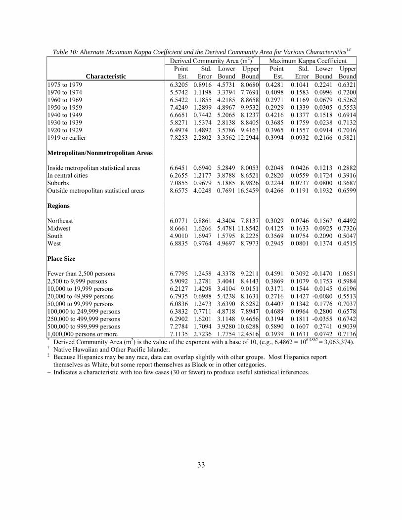
Table 10 Alternate Maximum Kappa Coefficient and the Derived Community Area for Various Characteristics14
Characteristic
Derived Community Area (m2) Maximum Kappa Coefficient Point
Est Std
Error Lower Bound
Upper Bound
Point Est
Std Error
Lower Bound
Upper Bound
1975 to 1979 63205 08916 45731 80680 04281 01041 02241 06321 1970 to 1974 55742 11198 33794 77691 04098 01583 00996 07200 1960 to 1969 65422 11855 42185 88658 02971 01169 00679 05262 1950 to 1959 74249 12899 48967 99532 02929 01339 00305 05553 1940 to 1949 66651 07442 52065 81237 04216 01377 01518 06914 1930 to 1939 58271 15374 28138 88405 03685 01759 00238 07132 1920 to 1929 64974 14892 35786 94163 03965 01557 00914 07016 1919 or earlier
MetropolitanNonmetropolitan Areas
78253 22802 33562 122944 03994 00932 02166 05821
Inside metropolitan statistical areas 66451 06940 52849 80053 02048 00426 01213 02882 In central cities 62655 12177 38788 86521 02820 00559 01724 03916 Suburbs 70855 09679 51885 89826 02244 00737 00800 03687 Outside metropolitan statistical areas
Regions
86575 40248 07691 165459 04266 01191 01932 06599
Northeast 60771 08861 43404 78137 03029 00746 01567 04492 Midwest 86661 16266 54781 118542 04125 01633 00925 07326 South 49010 16947 15795 82225 03569 00754 02090 05047 West
Place Size
68835 09764 49697 87973 02945 00801 01374 04515
Fewer than 2500 persons 67795 12458 43378 92211 04591 03092 -01470 10651 2500 to 9999 persons 59092 12781 34041 84143 03869 01079 01753 05984 10000 to 19999 persons 62127 14298 34104 90151 03171 01544 00145 06196 20000 to 49999 persons 67935 06988 54238 81631 02716 01427 -00080 05513 50000 to 99999 persons 60836 12473 36390 85282 04407 01342 01776 07037 100000 to 249999 persons 63832 07711 48718 78947 04689 00964 02800 06578 250000 to 499999 persons 62902 16201 31148 94656 03194 01811 -00355 06742 500000 to 999999 persons 72784 17094 39280 106288 05890 01607 02741 09039 1000000 persons or more 71135 27236 17754 124516 03939 01631 00742 07136 Derived Community Area (m2) is the value of the exponent with a base of 10 (eg 64862 = 1064862 = 3063374) dagger Native Hawaiian and Other Pacific Islander Dagger Because Hispanics may be any race data can overlap slightly with other groups Most Hispanics report
themselves as White but some report themselves as Black or in other categories ndash Indicates a characteristic with too few cases (30 or fewer) to produce useful statistical inferences
33
Conclusion
In this report I used data from the 2009 American Housing Survey in conjunction with
various GIS maps and tools to determine that the distance from the typical Americanrsquos house to
the edge of his community is between 520 and 1060 meters This derived community extent is
roughly equal to the radius of one or two median-sized census block groups Not surprisingly
condo communities and communities with 50 or more housing units per building are smaller than
communities of typical single family (detached) homes I also found a regional variation in
community size communities in the Midwest are larger than those in the South These findings
are not contradicted by an alternative method of deriving neighborhood size that accounts for
variations in the neighborhoodrsquos shape
34
References
Carroll T Clauretie T amp Neill H (1997) Effect of Foreclosure Status on Residential Selling
Price Comment Journal of Real Estate Research 13(1) 95-102
Cohen J (1960) A Coefficient of Agreement for Nominal Scales Educational and
Psychological Measurement XX(1) 37-46
Forgey F A Ronald R C amp VanBuskirk M L (1994) Effect of foreclosure status on
residential selling price Journal of Real Estate Research 9(3) 313ndash18
Frame W (2010) Estimating the Effect of Mortgage Foreclosures on Estimating the Effect of
Mortgage Foreclosures on Federal Reserve Bank of Atlanta Economic Review 95(3) 1shy
9
Immergluck D amp Smith G (2005) Measuring the effects of subprime lending on
neighborhood foreclosures Evidence from Chicago Urban Affairs Review 40 362ndash389
Immergluck D amp Smith G (2006 November) The Impact of Single-family Mortgage
Foreclosures on Neighborhood Crime Housing Studies 21(6) 851ndash866
Immergluck D amp Smith G (2006b) The External Costs of Foreclosure The Impact of Single-
Family Mortgage Foreclosures on Property Values Housing Policy Debate 17 57ndash79
Landis J R amp Koch G G (1977 March) The Measurement of Observer Agreement for
Categorical Data Biometrics 33(1) 159-174
Lin Z Rosenblatt E amp Yao V (2009) Spillover effects of foreclosures on neighborhood
property values Journal of Real Estate Finance and Economics 38(4) 387ndash407
Schuetz J Been V amp Ellen I G (2008) Neighborhood Effects of Concentrated Mortgage
Foreclosures Journal of Housing Economics 17 306ndash319
35
Taylor R B (2012) Defining Neighborhoods in Space and Time Cityscape A Journal of
Policy Development and Research 225-230
US Census Bureau (2011) Guide to State and Local Census Geography 2011 Retrieved
November 27 2012 from US Census Bureau
httpwwwcensusgovgeowwwguidestlocpdfAll_GSLCGpdf
US Census Bureau (2011) Current Housing Reports Series H15009 American Housing
Survey for the United States 2009 Washington DC 20401 US Government Printing
Office
US Dept of Housing and Urban Development (2012 November 14) Estimating AHS National
Variances with Replicate Weights Retrieved November 27 2012 from HUD USER
httpwwwhuduserorgportaldatasetsahsAHSN_Public_Use_Replicate_Weight_abbre
viated31OCT12pdf
36
Appendix A The Neighborhood Quality Section of the 2009 AHS
GATED The following questions are about your community Is your community surrounded by walls or fences preventing access by persons other than residents
1 Yes 2 No
GATEDV The following questions are about your community (Last time) we recorded that your community is surrounded by walls or fences preventing access by persons other than residents Is this information still correct
1 Yes 2 No
ACCESSC Does access to your community require a special entry system such as entry codes key cards or security guard approval
1 Yes 2 No
ACCESSCV (Last time) we recorded access to your community requires a special entry system such as entry codes key cards or security guard approval Is this information still correct
1 Yes 2 No
ACCESSB Does access to your building require a special entry system such as entry codes key cards or security guard approval
1 Yes 2 No
ACCESSBV (Last time) we recorded access to your building requires a special entry system such as entry codes key cards or security guard approval Is this information still correct
1 Yes 2 No
37
AGERES You mentioned that one or more members of your household are 55 or older Some communities are age-restricted meaning that at least one member of the family must be at least 55 years or older Is your development age-restricted
1 Yes 2 No
AGERESV (Last time) we recorded that your development was age-restricted meaning that at least one member of the family must be at least 55 years or older Is this information still correct
1 Yes 2 No
NORC Sometimes communities that are not age-restricted still attract certain age groups Do you believe the majority of your neighbors are 55 or over
1 Yes 2 No
CLUB Are any of the following features included in your community Community Center or Clubhouse
1 Yes 2 No
GOLF (Are any of the following features included in your community) Golf Course
1 Yes 2 No
TRAILS (Are any of the following features included in your community) WalkingJogging Trails
1 Yes 2 No
SHUTLE (Are any of the following features included in your community) Shuttle Bus
1 Yes 2 No
38
CARE (Are any of the following features included in your community) Day Care Center
1 Yes 2 No
BEACH (Are any of the following features included in your community) Beach Park or Shoreline
1 Yes 2 No
39
Appendix B Selected Statistics and Tabulation Area Counts by State
State Area (m2) Counts
Housing Units ZCTAs Census Tracts Block Groups Census Blocks Alabama 135767342446 2171853 629 1181 3438 252266 Alaska 1723336523156 306967 238 167 534 45292 Arizona 295232869248 2844526 362 1526 4178 241666 Arkansas 137731828968 1316299 504 686 2147 186211 California 423966968085 13680081 1719 8057 23212 710145 Colorado 269603398884 2212898 525 1249 3532 201062 Connecticut 14357375332 1487891 391 833 2585 67578 Delaware 6445769842 405885 67 218 574 24115 District of Columbia 176999744 296719 53 179 450 6507 Florida 170311608772 8989580 1028 4245 11442 484481 Georgia 153910578723 4088801 695 1969 5533 291086 Hawaii 28312992182 519508 95 351 875 25016 Idaho 216443477713 667796 206 298 963 149842 Illinois 149995304656 5296715 1381 3123 9691 451554 Indiana 94326221957 2795541 731 1511 4814 267071 Iowa 145745891267 1336417 684 825 2630 216007 Kansas 213099965684 1233215 561 770 2351 238600 Kentucky 104655683036 1927164 605 1115 3285 161672 Louisiana 135656018836 1964981 571 1148 3471 204447 Maine 91634122036 721830 432 358 1086 69518 Maryland 32131089610 2378814 491 1406 3926 145247 Massachusetts 27335741928 2808254 331 1478 4985 157508 Michigan 250486780758 4532233 987 2813 8205 329885 Minnesota 225161404423 2347201 798 1338 4111 259777 Mississippi 125455713880 1274719 382 664 2164 171778 Missouri 180540279352 2712729 1231 1393 4506 343565 Montana 380832074499 482825 361 271 842 132288 Nebraska 200328701612 796793 654 532 1633 193352 Nevada 286380145586 1173814 242 687 1836 84538 New Hampshire 24214215247 614754 194 295 922 48837 New Jersey 22591379380 3553562 595 2010 6320 169588 New Mexico 314917547864 901388 309 499 1449 168609 New York 141296785159 8108103 1793 4919 15464 350169 North Carolina 139390789884 4327528 833 2195 6155 288987 North Dakota 183107810720 317498 526 205 572 133769 Ohio 116097706996 5127508 1224 2952 9238 365344 Oklahoma 181037235141 1664378 633 1046 2965 269118 Oregon 254799589926 1675562 458 834 2634 196621 Pennsylvania 119280059748 5567315 1853 3218 9740 421545 Rhode Island 4001234100 463388 175 244 815 25181 South Carolina 82932660230 2137683 363 1103 3059 181908 South Dakota 199728851315 363438 443 222 654 88360 Tennessee 109153130302 2812133 811 1497 4125 240116 Texas 695661526826 9977436 2012 5265 15811 914231 Utah 219884162541 979709 288 588 1690 115406 Vermont 24906267580 322539 309 184 522 32580 Virginia 110786551025 3364939 826 1907 5332 285762 Washington 184661284315 2885677 630 1458 4783 195574 West Virginia 62756019147 881917 835 484 1592 135218 Wisconsin 169634848618 2624358 749 1409 4489 253096 Wyoming 253334294812 261868 177 132 410 86204 Totaldagger 9833536823091 131704730 32990 73057 217740 11078297
dagger ZCTAs do not cover all areas of the United States the total area of ZCTAs is 7592175985321 m2 Source TIGERLine Shapefiles 2012 US Census Bureau Geography Division
40
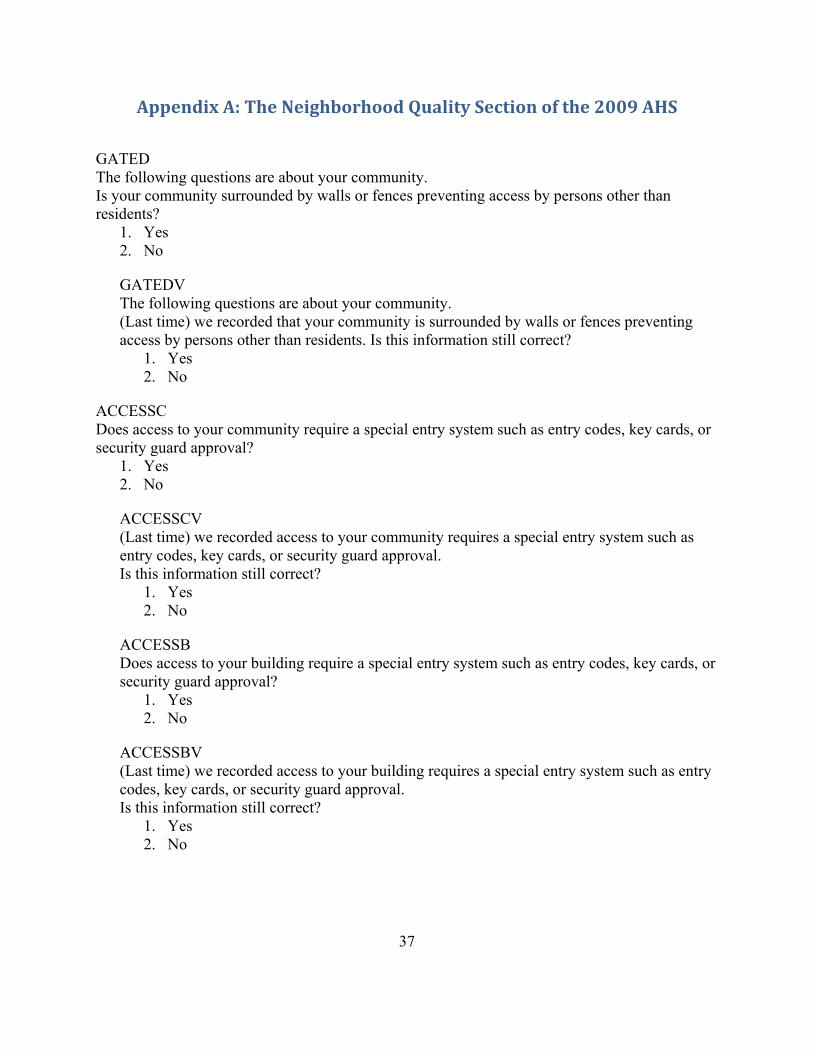
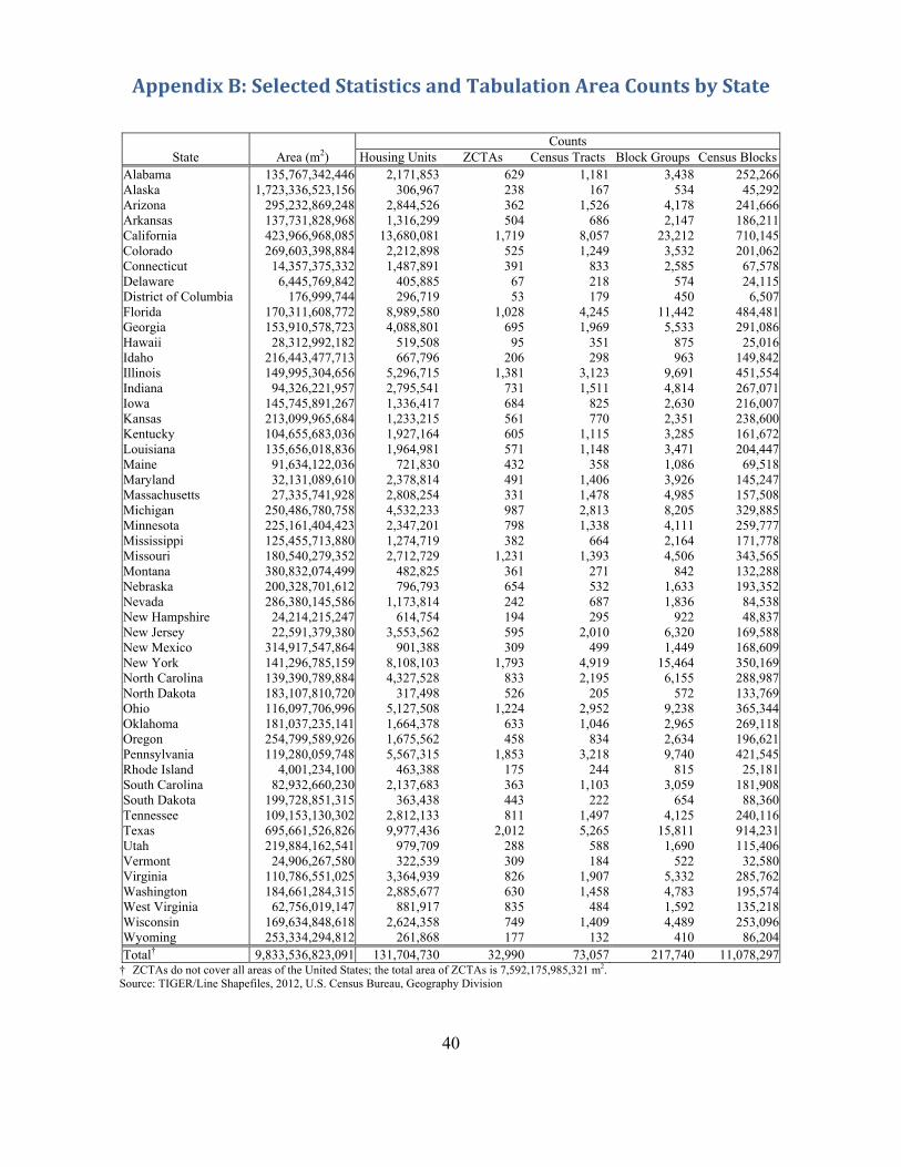