Embed Size (px)
Citation preview

João Pedro da Rocha Ferreira
How commuting influences urban economies and the environment:
A Commuting Satellite Account applied to the Lisbon Metropolitan Area
PhD Thesis in Sustainable Energy Systems, supervised by Professor Pedro Ramos and Professor Luis Cruz,
submitted to the Department of Mechanical Engineering, Faculty of Sciences and Technology of the University of Coimbra
June 2016
Vasco da Gama Bridge, FH Mira, licensed under the Creative Commons Attribution-Share Alike 2.0 Generic license.


�
�
�
João Pedro da Rocha Ferreira
PhD Thesis in Sustainable Energy Systems,
University of Coimbra
Energy for Sustainability (EfS/MIT Portugal Program)
Supervisors
Professor Doutor Pedro Ramos
Professor Doutor Luís Cruz
Coimbra, June 2016�
This work has been undertaken under the Energy for Sustainability Initiative of the University of
Coimbra and supported by FCT through the MIT-PORTUGAL program and the doctoral grant
FCT-DFRH-SFRH/BD/76357/2011, as well as by the R&D Project EMSURE - Energy and Mobility
for Sustainable Regions (CENTRO-07-0224-FEDER-002004).


i
“If I came this far, it is by standing on the shoulders of giants.”
Isaac Newton, adapted
“One's destination is never a place, but a new way of seeing things.” Henry Miller
Acknowledgments
What a journey! More than 5 years (or exactly 2022 days). What an incredible expedition,
a wonderful wife, a marvelous wedding, a fantastic family, the best supervisors, so many
inspiring friends, and such promising students. Thank you all! It was a true challenge and it
has been very difficult at times, but now it is so rewarding!
Without doubt, the pages in this dissertation only express a small proportion of the
moments, meetings, conversations, feelings, conferences, smiles, dinners, wines and journeys
that made this outcome possible. To Professor Pedro Ramos, Professor Luis Cruz and
Professor Eduardo Barata, for being (much) more than supervisors, for your friendship and
for the tremendous effort, work and enormous amount of hope you put into this work, I will
be always grateful. To my wife, for making me one happy guy and for being so patient in the
most difficult moments - I promise in the next years I will try to compensate you with dinners,
travel and the tones of affection you deserve. To my family, particularly my parents, for
making this possible - your inspiring example, irreplaceable teaching and giant struggle to
give me the conditions to achieve my goals are just unutterable (which for an economist is a
real thing). To Professor António Martins and those involved in EMSURE and in the EfS
Initiative for making it so easy and interesting to be part of this research project management.
To all my colleagues in FEUC, particularly those involved in the Masters in Local Economics,
for giving me the will to go further and pursue a PhD. To the brilliant inspiring persons I had
the opportunity to meet during these years and for their remarkable contributions to my work:
Geoffrey Hewings, Michael Lahr, Eduardo Haddad, Joaquim Guilhoto and Jorge Carvalho.
Thank you Rui Pina for all the beers, the parties and the GIS teachings. Gil Ribeiro for the
barbecues and land-policy talks. João Miranda and Pedro Nunes, sorry for ruining
innumerous nights in the Tropical talking about work and commuting - I will give you a rest
in the future. To Filipe Silva, for the innumerable cigarettes and coffees until the small hours,
when we tried to solve the world’s economic problems.
To Inês S., Rafael F., Ana P., Pedro P., Inês C., Alfredo C., Ana M., Nuno B. and Nuno
P. just for the “huge” thing of always being there for me. To my parents-in-law for all the
friendship and for being the parents of a terrific woman. To all those in ABIC who stand for
better conditions for young Portuguese researchers. To my students - you made me a better
person. To Clare Sandford, by her proofreading.
You are the giants where I am seated.

ii
Abstract
The world is becoming more and more urbanized. The growth of megacities has been
intrinsically linked with increasing sprawling that compels millions of workers to commute.
Commuting has often been either neglected or simply viewed as a byproduct of the markets
operating and individual choices. However, as a mass phenomenon, commuting has benefits and
costs well beyond those supported by each individual, which further shape urban and regional
economies.
This PhD dissertation sets out a proposal for an innovative Commuting Satellite Account
(CSA). This framework integrates into a Multi-Regional Input-Output (MRIO) model five main
elements that arise from commuting: (1) commuting flows are represented in a specific
geographic and economic context; (2) commuting influences the regional distribution of income;
(3) commuting affects household consumption structures; (4) commuting is intrinsically linked
with the rental prices of housing and business premises; and, (5) commuting is a major cause of
energy consumption and CO2 emissions.
To assess commuting opportunity costs, the CSA extension to the MRIO framework is applied,
as an illustrative example, to the Lisbon Metropolitan Area. Two hypothetical extreme scenarios
are considered, both assuming that commuters change their status to non-commuters: one by
considering the change of their place of residence to the municipality where they work; and the
other one by assuming that the corresponding production activities are displaced to the suburbs.
The CSA is also empirically tested in a more ‘realistic’ case, providing important insights into a
scenario of commuting reduction resulting from a strategy of urban recentralization.
The comprehensive analysis of these applications indicates dichotomous, yet complementary,
conclusions: commuting, by itself, induces significant economic, social and environmental costs,
although commuting, as one of the many elements associated with the agglomeration
phenomenon, is undoubtedly linked to increasing productivity and economic growth. To
conclude, this work discusses the adoption of policy oriented recommendations, either through
actual urban planning application, or by resorting to land-use and transport policy instruments,
which might contribute to refrain sprawling in metropolitan regions and intervene to achieve the
broader aims of economic growth, well-being and a more sustainable urban environment.
Keywords: Commuting, Environmental Impacts, Metropolitan Areas, Multi-Regional
Input-Output, Satellite Account, Travel Patterns, Urban Policy, Urban Sprawling.


iii
Resumo
O mundo está a ficar cada vez mais urbanizado. O crescimento de megacidades está
intrinsecamente ligado à sua expansão territorial, obrigando milhões de trabalhadores a efetuarem
deslocações pendulares. Esta atividade tem sido geralmente ignorada ou considerada apenas como
um resultado do funcionamento do mercado e das escolhas dos indivíduos. No entanto, sendo um
fenómeno generalizado, o volume diário de deslocações pendulares tem benefícios e custos que
vão para além dos suportados pelos indivíduos, contribuindo para moldar as economias urbanas
e regionais.
Esta Dissertação de Doutoramento propõe uma Conta Satélite de Commuting (CSC). Este
elemento inovador é integrado num modelo Multi-Regional de Input-Output (MRIO),
incorporando cinco componentes ligadas às deslocações pendulares: (1) os fluxos pendulares são
representados num contexto geográfico e económico específico; (2) as deslocações pendulares
influenciam a distribuição regional de rendimento; (3) as deslocações pendulares afetam a
estrutura de consumo das famílias; (4) as deslocações pendulares estão intimamente relacionadas
com o valor das rendas de habitação e de escritórios e outros edifícios usados pelas empresas; e,
(5) as deslocações pendulares estão na origem de elevados níveis de consumo de energia e de
emissões de CO2.
Para estimar os custos de oportunidade das deslocações pendulares, aplica-se a CSC à Área
Metropolitana de Lisboa. Para o efeito consideram-se dois cenários (extremos) hipotéticos, que
apontam o fim das deslocações pendulares: um admite a alteração do local de residência dos
trabalhadores para o município onde trabalham; o outro assume que uma parte da atividade
produtiva é deslocada para a periferia, onde os trabalhadores residem. A CSC é também testada
num exercício mais ‘realista’, permitindo avaliar potenciais impactos associados a situações em
que as deslocações pendulares se reduzam como resultado da aplicação de uma estratégia de
centralização urbana. A análise detalhada dos resultados deste trabalho aponta para conclusões
dicotómicas, ainda que complementares: as deslocações pendulares, por si, induzem importantes
custos económicos, sociais e ambientais; no entanto, as deslocações pendulares, enquanto
elemento associado à aglomeração urbana, estão relacionadas com o aumento da produtividade e
o crescimento económico. Para concluir, este trabalho discute a implementação de políticas de
planeamento urbano e o uso de instrumentos de política do solo e de transportes. Estas soluções
poderão contribuir para conter a dispersão territorial das cidades e concretizar objetivos de
crescimento económico, bem-estar e de um melhor e mais sustentável ambiente urbano.
Palavras-chave: Contas Satélite; Deslocações Pendulares, Expansão Urbana; Impactos
Ambientais; Multi-Regional Input-Output; Padrões de Mobilidade; Planeamento Urbano


iv
Table of contents
CHAPTER 1 – Introduction .......................................................................................... 1
1.1. Research Motivation .............................................................................................. 1
1.2. Commuting – a Multi-dimensional Phenomenon .................................................. 5
1.2.1. Commuting, Sprawling and Economic costs .................................................. 9
1.2.2. Commuting, Income Distribution and Consumption Preferences ................ 11
1.2.3. Commuting and Real Estate Market ............................................................. 13
1.2.4. Commuting, Energy Consumption and CO2 emissions ................................ 16
1.2.5. Commuting and Input-Output models: overcoming research gaps ............... 17
1.3. Research Gap(s) and Dissertation Structure ........................................................ 21
CHAPTER 2 - The Lisbon Metropolitan Area: economic activity and the
commuting phenomenon .............................................................................................. 25
2.1. Introduction .......................................................................................................... 25
2.2. The Lisbon Metropolitan Area ............................................................................ 26
2.3. Results of the International and Interregional Trade Estimations ....................... 31
2.4. Commuting activity in Portugal and in the LMA ................................................ 37
2.5. Final Comments ................................................................................................... 50
CHAPTER 3 – Multi-Regional Input-Output Models .............................................. 53
3.1. Introduction .......................................................................................................... 53
3.2. MULTI2C – Shaping a Portuguese National Matrix for Impact Assessment ..... 55
3.2.1. From purchaser to basic prices ...................................................................... 59
3.2.2. From total to domestic flows ......................................................................... 61
3.2.3. A ‘Closed’ I-O Model ................................................................................... 63
3.2.3.1. Households Consumption ....................................................................... 63
3.2.3.2. Households income................................................................................. 65


v
3.3. MULTI2C – Deriving Regional Matrices ........................................................... 68
3.3.1. Regional Products Supply ............................................................................. 68
3.3.2. Regional Intermediate Consumption ............................................................. 70
3.3.3. Regional Households Income and Consumption .......................................... 71
3.3.4. Regional Other Final Demand and GVA Components ................................. 73
3.4. MULTI2C - MRIO Matrices and Interregional Trade ......................................... 74
3.5. Stepping Forward: A LMA Tri-regional I-O Model............................................ 80
3.5.1. Deriving Regional Matrices and Trade estimations ...................................... 80
3.6. Final Comments ................................................................................................... 82
CHAPTER 4 – Commuting Satellite Account: Concept, development and
applications ................................................................................................................... 83
4.1. Introduction .......................................................................................................... 83
4.2. A ‘traditional’ MRIO approach ........................................................................... 85
4.3. Regional Income Distribution .............................................................................. 90
4.4. Household consumption structures: commuters vs non-commuters ................... 93
4.5. Real Estate Rental Activities ............................................................................... 98
4.6. The Final Framework of the Commuting Satellite Account .............................. 104
4.7. A Rectangular I-O Model based on the CSA Framework ................................. 107
4.7.1. A General Procedure ................................................................................... 107
4.7.2. Integrating the Energy / Environmental Satellite Account ......................... 111
4.8. Assessing Commuting (Opportunity) Costs in the LMA .................................. 113
4.8.1. Deriving Two “Extreme” Scenarios ............................................................ 113
4.8.2. Scenario Results: The Economic, Social and Environmental Impacts of
Commuting ............................................................................................................ 115
4.8.3. Changes in real estate rents ......................................................................... 120
4.9. A ‘wasteful commuting’ reduction scenario ...................................................... 123


vi
4.10. Applying a CSA modelling framework: ‘commuting embodied’ in product
production ................................................................................................................. 126
4.11. Final Comments ............................................................................................... 131
CHAPTER 5 – Conclusion ........................................................................................ 133
5.1. Methodological and empirical contributes ........................................................ 134
5.2. Policy Recommendations................................................................................... 139
5.3. Limits and Future Research ............................................................................... 143
5.4. Final Words ........................................................................................................ 145
REFERENCES ........................................................................................................... 133


vii
Index of Tables
Table 1: Share of Gross Value Added by industries in each Portuguese NUTS II region (2010) .................................................................................................................. 28
Table 2: Location quotients by Portuguese NUTS II region and by industries (2010) ............................................................................................................................. 29
Table 3: Top 5 and bottom 5 location quotients of industries among the two NUTS III regions in the Lisbon Metropolitan Area (2010)............................................ 30
Table 4: Trade Balance of Greater Lisbon and Peninsula de Setubal (2010)................. 32
Table 5: Most important products (ranked by Net-Exports volume (106 €)) in Greater Lisbon and Peninsula de Setubal (2010) ........................................................... 33
Table 6: Nights spent in hotel establishments (103) by non-residents in Portugal by region (2010) .................................................................................................................. 34
Table 7: 10 most important products produced in Greater Lisbon in terms of (only) Interregional net-Exports (2010) ......................................................................... 35
Table 8: 10 most important products produced in Peninsula de Setubal in terms of (only) Interregional net-Exports (2010) ......................................................................... 36
Table 9: Overall Interregional Gross and Net exports (106 € and % of GDP) from Greater Lisbon, Peninsula de Setubal and Rest of the Country (2010) .......................... 37
Table 10: Commuting Patterns among Portuguese employed resident population (2011) ............................................................................................................................. 38
Table 11: Distribution of commuters and non-commuters, by place of residence, among the Portuguese NUTS III regions (2011) ............................................................ 39
Table 12: Share of workers, by place of residence, which commute to other NUT III region (2011) ............................................................................................................. 41
Table 13: Portuguese workers origin-destiny matrix (2011) .......................................... 41
Table 14: LMA demographic indicators, employment and share of commuters by municipality (2011) ........................................................................................................ 43
Table 15: Number of kilometers (103) travelled by commuters per day by the LMA workers/residents (2011) ...................................................................................... 46
Table 16: Daily average kilometers (103) traveled by commuters working or living in the LMA (2011) .......................................................................................................... 46
Table 17a: Industries attracting more and less commuters in Greater Lisbon according with the place of residence of the workers .................................................... 47
Table 17b: Industries attracting more and less commuters in Peninsula de Setubal according with the place of residence of the workers .................................................... 48
Table 18: Modal split in Lisbon Metropolitan Area and in the Rest of Country according with the different travel patterns .................................................................... 49


viii
Table 19: Average time spent (in minutes) on commuting by means of transport and by region of residence (2011) .................................................................................. 50
Table 20: Products yielding to Trade margins................................................................ 60
Table 21: Products yielding to Transportation margins ................................................. 61
Table 22: Household consumption structure by main source of income, at national level, at purchaser’s prices.............................................................................................. 64
Table 23: Share of household types in the national distribution of labor income (2010) ............................................................................................................................. 90
Table 24: Income distribution by region (106 €) ............................................................. 92
Table 25: Income in and outflows by region (106 €) ...................................................... 92
Table 26a: Petrol consumption (commuting-responsibility) of commuters living or working in the LMA (103 €) ........................................................................................... 96
Table 26b: Diesel consumption (commuting-responsibility) of commuters living or working in the LMA (103 €) ....................................................................................... 96
Table 26c: LPG consumption (commuting-responsibility) of commuters living or working in the LMA (103 €) ........................................................................................... 96
Table 27: Commuters’ and non-commuters’ consumption structures (total flows, at purchasers’ prices) ...................................................................................................... 97
Table 28: Renting-flows: Origin-Destination (2010) ..................................................... 99
Table 29a: Renting-flows – Origin-Destination according to building location at regional level (2010) ..................................................................................................... 100
Table 29b: Renting-flows – Origin-Destination according to the place of residence of the building-owner at the regional level (2010) ....................................................... 100
Table 30a: Origin-destination rent flows received by firms (106 €) ............................. 102
Table 30b: Origin-destination rent flows received by households (106 €) ................... 102
Table 31: Distribution of the rents paid to households, by households’ main income source (2010) ................................................................................................... 103
Table 32: Multi-dimensional impacts of Scenarios A and B........................................ 117
Table 33: Industries that decline more in relative terms of national GVA (in Scenario A) ................................................................................................................... 118
Table 34: Industries located in Greater Lisbon that have a relatively higher increase in their GVA (in Scenario A) ......................................................................... 119
Table 35: Sensitivity Analysis of Real Estate Rent Changes (national values) ........... 121
Table 36: Household Income changes (%) resulting from the sensitivity analysis of real estate rent changes (national values) ................................................................. 122
Table 37: Greater Lisbon household types redistribution ............................................ 124
Table 38: Impacts of occupying 50% of the ‘unoccupied’ houses in Lisbon municipality .................................................................................................................. 125
Table 39: Commuting ‘embodied’ in 1% of product production in Greater Lisbon: Top 6 products .............................................................................................................. 130


ix
Index of Figures
Figure 1: Map of Portugal and Lisbon Metropolitan Area ............................................. 27
Figure 2: Share of commuters in the employed resident population, by
municipality (2011) ........................................................................................................ 40
Figure 3: Commuting flows in the Lisbon Metropolitan Area (2011) ........................... 44
Figure 4: Share of employed population working in the municipality of Lisbon, by
place of residence (2011) ................................................................................................ 45
Figure 5: National matrix at purchasers’ prices and total flows ..................................... 57
Figure 6: Portuguese matrix at “basic prices” and “domestic flows”............................. 62
Figure 7: Portuguese matrix, at “basic prices” and “domestic flows”, and ‘closed’
to households mainly living from labor .......................................................................... 67
Figure 8: “Cascade-stepwise” derivation of the MRIO flows and matrices .................. 81
Figure 9: Bi-regional Input-Output model derived from the
MULTI2C framework .................................................................................................... 86
Figure 10: The structure of the Commuting Satellite Account .................................... 105


João Pedro da Rocha Ferreira
How commuting influences urban economies and the environment?
A Commuting Satellite Account applied to the Lisbon Metropolitan Area
PhD Thesis in Sustainable Energy Systems,
supervised by Professor Pedro Ramos and Professor Luis Cruz
March 2016
Vasco da Gama Bridge, FH Mira, licensed under the Creative Commons Attribution-Share Alike 2.0 Generic license.


“Imagination is more important than knowledge. For knowledge is limited to all we now know and understand, while imagination
embraces the entire world,
and all there ever will be to know
and understand.”
Albert Einstein, 1929
CHAPTER 1 – INTRODUCTION
1.1. Research Motivation
The world is becoming more and more urbanized. Nowadays, cities are the home of
more than 50% of the world’s population. This number is expected to rise to 70% by 2050
(UN, 2014). Urbanization has several consequences that are the subject of strong debate,
full of controversial and antagonistic opinions, about the (dis)advantages of this
phenomenon. Despite such intense and passionate debate, it seems unquestionable that
given the recent progress towards a borderless world economy, cities have been
enhancing their importance as the basic units of economic systems (Fujita, 1999). Cities
are engines of national and global growth, accounting for around 80% of global economic
output. The world’s 150 largest metropolitan economies produce 41% of global GDP with
only 14% of global population (Floater et al., 2014). The viability of megacities and large
metropolitan areas has been intrinsically associated with the admirable technological and
societal advances that allow humans to live together in confined buildings or territories1
and cities to sprawl for several miles while still providing basic services (e.g. water,
1 When the Chrysler Building was built in 1930 in New York, USA, it was the tallest building in the world
at 319 meters. Now, there are 30 buildings in the world that are taller than the Chrysler Building.

CHAPTER 1 – INTRODUCTION
2
electricity, waste collection). Indeed, this reality is only possible because of lower
transportation costs, which allow people to travel larger distances within urban areas and
commute longer distances daily between their home and work.
Commuting has often been “either neglected or typically seen as the market working
just fine” (Ewing, 1997). In a more ‘traditional’ economic view, if commuting is seen as
the cost of time and distance, then commuting is only an option if it is compensated by
either a rewarding job or by additional welfare gained from a pleasant living environment.
Accordingly, commuting is the consequence of an equilibrium state between the housing
and labor market, in which individuals’ utility (or well-being) is maximized given all of
the combinations of alternatives in these two markets.2 This conclusion, which is based
on a more individualistic approach, is not consensual among economists and other social
scientists, as they question the possibility of individuals making rationale choices
associated with commuting (Hamilton and Röell, 1982; Stutzer and Frey, 2008).
Additionally, it is also possible to address the commuting phenomenon as a social and
widespread activity with an influence that goes far beyond the strict analysis of each
individual’s choice and well-being. As with any mass phenomenon, the benefits and costs
supported by each individual can be critically different from those supported by the
society as a whole. Thus, commuting is a means of providing a vital input (workforce)
into production activities and is simultaneously a mandatory routine for working
households to secure their income. Indeed, it is indisputable that the growth of commuting
has made a critical contribution to stretching urban areas’ boundaries and to exacerbating
energy consumption and greenhouse gas emissions. Furthermore, commuting plays a
central role in regional and urban economies as it shapes the social, economic and
environmental dimensions of metropolitan areas. In short, it requires the application of
more holistic approaches.
This PhD dissertation addresses the topic of commuting by proposing a methodology
suitable for assessing its multi-dimensional impacts. For this, a set of interactions are
characterized by gathering and systematizing several statistical data and incorporating
such information into a Multi-Regional Input-Output (MRIO) framework. This modeling
2 The efficient allocation of resources has been studied, based on the conviction set forth by Wildasin
(1987: 1136) that “migratory flows will arbitrage away any utility differentials among jurisdictions. Therefore, it is appropriate to impose equal utilities as a constraint at the outset, and to ask what allocation of resources will maximize the common level of utility for all households.”

CHAPTER 1 – INTRODUCTION
3
framework can accurately describe the interactions between industries and households
located in specific regional contexts within metropolitan areas.
Then, an additional set of transformations is proposed to perform a more realistic
assessment of commuting. These specific transformations, incorporated together, are the
core of the proposed ‘Commuting Satellite Account’ (CSA). This is an extension of
MRIO models that embrace five critical dimensions of commuting, namely:
(1) commuting flows are represented in a specific geographic and economic
context;
(2) commuting influences the regional distribution of income;
(3) commuting affects household consumption structures;
(4) commuting is intrinsically linked with the rental prices of housing and business
premises;
(5) commuting is a major cause of energy consumption and CO2 emissions.
These dimensions are widely acknowledged in the literature but the design of a
modeling framework capable of incorporating all of them within the economic context of
a specific region is still missing from regional and urban economic studies. Indeed, the
design of this model preceded the major goal and motivation of this work: assessing the
multi-dimensional impacts of commuting in metropolitan areas through the application
of the CSA framework in a real world case study.
Accordingly, this model is applied to the Lisbon Metropolitan Area (LMA), the most
densely populated urban region in Portugal. Commuters are defined as all of the people
living in one municipality and traveling daily to another municipality for the purpose of
working, as employees or on their own account. One of the purposes of this work is to
appraise the opportunity costs (or benefits) of commuting. For that, two ‘major’ scenarios
are applied in the context of the CSA modeling framework. One consists of hypothetically
relocating the commuters’ place of residence to the place where they work, while the
other involves a hypothetical redistribution of the industries’ economic activity,
according to the place where commuters live. Both scenarios involve commuting ceasing
and represent the counterfactual to the current reality. This will allow for testing the
hypothesis that the geographical distribution of people and human activities is not neutral
and may induce a loss or a benefit that the society should consider. These scenarios are
complemented by a more ‘realistic’ application concerning the return of a feasible
quantity of commuters to live in the CBD. Accordingly, this set of contributions is

CHAPTER 1 – INTRODUCTION
4
expected to enlighten future academic works and decision makers with regard to the role
of commuting in shaping urban economies.
For decades, commuting and urban expansion development have been systematically
ignored in terms of oriented policy recommendations (Ewing, 1997; Carvalho, 2013). In
many countries, including Portugal, urban planning has been focused essentially on
municipal legislation with a lack of coordination and regulatory measures applied at more
macro levels (e.g. metropolitan or regional level)3. This fact has contributed to the
absence of coherent urban policies at the metropolitan level (e.g. concerning land-use
regulations or transportation network planning) and promoted competition by attracting
population between local governments. In Portugal, this fact is even more relevant as two
of the main municipality revenues are associated with extensive land-use, namely the
Municipal Tax over Real Estate (supported by house owners) and the cos ton licensing
new buildings and constructions. So, the suburbia municipalities of the CBDs, which
could already afford lower land costs, are also interested in attracting more and more
inhabitants. Therefore, as described by Wyly et al. (1998), municipalities compete with
each other in order to capture the largest amount of taxes.
All of this ‘apparent neutrality’ towards commuting, promoted by some governmental
and political institutions, has contributed to a situation where commuting prevails and
will probably continue to be more and more relevant in the future. Undoubtedly, a new
perception of commuting can have a decisive role in supporting policy designed to
accomplish the 11st Sustainable Development Goal of the UN 2030 Agenda, which calls
upon world leaders to make cities and all “human settlements inclusive, safe, resilient,
and sustainable” (UN, 2015). So, the proposed CSA framework is expected to be a
decisive step towards a deeper understanding of this complex phenomenon.
This PhD dissertation was developed in the scope of the PhD program in Sustainable
Energy Systems and the Energy for Sustainability initiative (Batterman et al., 2011). The
work presented here is the result of a proficuous period in which the author of this
dissertation participated in two research projects, and was author and co-author of seven
articles in international journals, two articles in national journals, two book chapters, 32
papers published in Conference Proceedings and two awards.
3 According to Newman and Thornley (1996: 53) “the municipalities (…) are the centers of regulatory
planning power and once they have an approved municipal plan, which is a comprehensive plan for physical and socio-economic development and covers their whole area, they can prepare more detailed plans. There are the more detailed urban plans for parts of the area and also detailed layout plans, which involve the parishes”.

CHAPTER 1 – INTRODUCTION
5
This first section offers the ‘foundations’ that established the motivation for this PhD
dissertation and addresses this particular ‘societal challenge’. Following that, this chapter
is devoted to the discussion of the most important works that have decisively contributed
to establishing the motivation and methodology embraced in this work. Next, the chapter
concludes by pinpointing the research gap(s) and presenting the structure of this PhD
dissertation.
1.2. Commuting – a Multi-dimensional Phenomenon
Commuting has been identified as the activity performed by those people that
periodically, as a rule on a daily basis, travel between their place of residence and
workplace4 and by doing this surpass the boundary of their residential community. In the
scientific literature, the word commuting can be preceded by an adjective that can imply
a more specific meaning (e.g., long distance commuting, green commuting, sustainable
commuting).
The term “commute” etymologically derives from the Latin commutare, meaning “to
often change, to change altogether” from com (intensive prefix) plus mutare “to change”.
According to Paumgarten (2007), in the 1840s the men who rode the railways each day
from the newly established suburbs to work in the cities did so at a reduced rate by buying
the so-called commutation ticket. Those people were the commuted. A few years later,
linguistic evolution transformed the commuted into commuters. In New York, and in
cities like Philadelphia, Boston and Chicago, railways (and the investment in transport
networks) improved the desirability of the suburbs. So, by the time the automobile
emerged a new way of living had already been established. It was with this kind of
commuting that people became familiarized with, despite the number of “negative”
effects.
The complementary effects of commuting have been well documented in the past.
Writers such as John Cheever or Richard Yates included several passages in their novels
portraying the life of typical American workers in New York and other metropolitan cities
and their clipped conversations on the platform, the new airy houses as an aspiration of
the American dream, the fraught encounters in moving cars, and the grooved route
between city and country, each a terminus of both entrapment and escape (Tanenhaus,
4 In this work commuting is limited to those that work; however in some circumstances commuting can
also include a reference to students.

CHAPTER 1 – INTRODUCTION
6
2015). After flourishing in the 19th and at the beginning of the 20th century, commuting
has not stopped growing. The opinions and “emotional” positions regarding commuting
are so vast and differentiated that ignoring commuting and its implications is no longer
possible. Accordingly, urban planning, environmental issues and urban governance have
become more and more challenging. Yet, a general agreement looks far from possible.
“Commuting, in the sense of using some form of transportation to separate one’s places of work and rest, is – in theory at least – a rational exercise. It allows people,
if not to have the best of both worlds, to achieve the best of all compromises: a
rewarding job and a pleasant home. The travelling itself is the price that has to be
paid to realize these two goals. It requires commuters to surrender their liberty to
the operators of public transport, or to congestion on the roads, while they cross a
kind of no man’s land, whose interim stations or junctions are measures of their progress – no more – and which they’d probably never visit for their own sakes” (Gately, 2014).
“Given the loss of personal well-being generally associated with commuting, the
results suggest that other factors such as higher income or better housing may not
fully compensate the individual commuter for the negative effects associated with
travelling to work and that people may be making sub-optimal choices. This result
is consistent with the findings of previous studies such as Stutzer and Frey (2008).
This is potentially important information both for those who commute, particularly
for an hour or more, and for their employers” (Office for National Statistics - UK, 2014).
With such remarkable and profound roots in the daily life of every urban citizen, the
references to scientific works with “commuting” as a keyword cross all areas of expertise
from arts to economics or mathematics. From the scientific publications referenced in
“ScienceDirect”,5 more than 300 have “commuting” as one of their keywords.6 40% of
these articles were published in journals devoted to energy and environmental sciences,
20% to engineering, computer and decision sciences, 19% to economics and business and
finance and 3% to arts and humanities. The remaining share (18%) belong to the other
social and exact sciences (namely medical sciences). A quantitative analysis of the most
common keywords associated with commuting shed light on the dimensions that more
often go along with papers concerning studies on this topic, namely:
(1) the relevance of the geographical and territorial dimension where commuting
actually happens (e.g., Central Business District, Urban, City, Rural, China, Hong
Kong, Brussels);
5 A webpage search engine that serves as a platform for access to nearly 2,500 academic journals and over
26,000 e-books. 6 Searched in 15th March, 2016.

CHAPTER 1 – INTRODUCTION
7
(2) activities, household types and complementary subjects associated with
commuting (e.g., job, travel, household, student, worker, labor market, housing
market);
(3) the different means of transportation used by commuters (e.g., bus, bicycle,
automobile, public transport, accessibility);
(4) references to commuting externalities or other consequences (e.g., energy
consumption, resource consumption, CO2 emissions, physical activity);
(5) methodological solutions to addressing commuting issues (e.g., model, choice,
urban economics, individual preferences; urban planning);
So, although Economics represents a small share of the scientific publications
associated with commuting, a simple reading of the most related keywords highlights the
potential relevance of the topic to this discipline. Moreover, as a topic that has such a
rooted presence in people’s daily lives, it also matches perfectly as a subject of study
according to the definition of Economics proposed by Alfred Marshall, more than 120
years ago.
“Economics is a study of mankind in the ordinary business of life; it examines that
part of individual and social action which is most closely connected with the
attainment and with the use of the material requisites of wellbeing” (Marshall, 1890).
This ambition of applying Economics to the study of what is important to mankind,
together with the relevance of commuting, can be observed in the work of the Nobel
Laureate Daniel Kahneman7 together with Alan Krueger. In this study they performed a
survey and asked the respondents to rate several activities according to how much they
enjoyed them. Morning commuting was the least preferred activity; it was even less
preferred than “working” (Kahneman and Krueger, 2006). The study also concluded that
reducing the amount of time spent commuting was critical to improving the happiness of
this population8.
Another Nobel Laureate, Paul Krugman9 has also written a vast amount of scientific
literature in which commuting and urban concentration are an expression of intangible
forces. Krugman (1996) considers that these two dimensions are in permanent tension
7 Awarded with a Nobel Laureate in Economics in 2002. 8 Sandow (2014) shows that the implications of commuting can be so intense that separation rates are 40%
higher among long-distance commuting couples compared with non-commuting couples. 9 Awarded with a Nobel Laureate in Economics in 2008.

CHAPTER 1 – INTRODUCTION
8
due to centripetal and centrifugal forces (economies of scale, reduced transportation costs
and labor mobility) that push the city together and commuting (and its consequences),
which arises as the main diseconomy of a particular city. This new contribution from
Krugman in particular contradicts the neoclassical urban systems theory, which considers
that competition among city developers produces cities of optimal size in a perfect
equilibrium.10 Indeed, Krugman proves that the extent and direction of these forces are
very sensitive to the internal and external reality of a given metropolitan area and surely
need a more complex and realistic study.
So, despite the distinctive methods and objectives of the analysis, commuting has
emerged as an important point in the works of these two Nobel Laureates. On the one
hand, Kahneman showed how commuting can be critical in people’s lives and, on the
other, Krugman underlined a more structural and immaterial dimension of commuting
that contributes to shaping the economies and the territory. Both works were important at
an early stage of this work, as they contributed to establishing a more unambiguous
motivation and ambition for this work.
Together with the works of Kahneman and Krueger (2006) and Krugman (1995; 1997;
199911; 2001; and 2008), the works to be introduced in the next sub-sections have made
a considerable contribution to the motivation and definition of the general ambition of
this research work. Other works that were also quite important in the initial phase of this
research work are more devoted to understanding the cause(s) of commuting: e.g.,
housing prices (Malpezzi, 1996; Cameron and Muellbauer; 1998), accessibility through
public transit systems (Kawabata and Shen, 2007), education levels (Magrini and
Lemistre, 2013), gender (Kwan and Kotsev, 2014) and ethnicity (Williams et al., 2014).
In contrast, the option consisted of trying to address the consequences of commuting.
This section is divided into 5 sub-sections. The next sub-section is devoted to works
that have studied the economic costs associated with urban sprawled regions. Next, sub-
section 1.2.2. addresses the impact of commuting on interregional income distribution
and household consumption expenditure. The following sub-section is dedicated to the
relationship between commuting and housing costs. Next, sub-section 1.2.4. addresses
the negative externalities of commuting, namely those associated with the environment
and greenhouse gas emissions. Finally, the last sub-section explores the potential of
10 Moreover, another important critic to neoclassical urban systems theory is its non-spatial nature. While
describing the number and types of cities, nothing is said about their locations. 11 Co-authored with Fujita and Mori.

CHAPTER 1 – INTRODUCTION
9
Input-Output (I-O) and MRIO models to assess this kind of multi-dimensional
approaches.
1.2.1. Commuting, Sprawling and Economic costs
In this sub-section, several studies relating urban forms with specific costs supported
by society are addressed. These studies have the key characteristic of considering that
commuting must be applied by models capable of linking geography and economics.
The discussion comprising the economic and environmental impacts of different urban
forms had its first contribution in The Costs of Sprawl (RERC, 1974), which was a
determinant in launching a debate that still persists. The goals established in this study
were focused on addressing the question of how the distribution of human activities
influences the economic costs supported by governments or other economic agents in the
provision of different services (such as, e.g. recreation, schools, roads, street lighting,
infrastructures and other several utilities). Their conclusion referred to the fact that
sprawling had higher economic and environmental costs12 than a more concentrated urban
region. Other studies, however, published subsequently have contradicted this idea.
Muller (1975) and Windsor (1979) argue that some sprawling benefits were not accessed
in these works.13 This intense debate has persisted with TCRP (1998) and Mandelker
(1998) making important contributions to reinforcing the original conclusions of the
RERC (1974) study.
Despite the different conclusions, an effort has been made to understand the overall
impacts, which can vary accordingly with the geographical configuration of a given area.
Gordon and Richardson (1997) identified 16 different costs associated with urban
sprawling and organized them into 5 major areas: Transportation and Travel Costs,
Public-Private Capital and Operating Costs, Land and Natural Preservation, Quality of
Life and Social Effects. They did not conclude that there was any relation between the
majority of these costs (except in the specific case of Transportation and Travel costs)
and the different urban forms. Accordingly, Small and Gómez-Ibáñez (1997) and
12 Namely the pollutants resulting from car use (measured in gallons per day), sewage effluent (liters per
year) and water use (gallons per year) (RERC, 1974) 13 It is important to note that the proper identification and quantification of the urban forms is not
straightforward. E.g. Ewing et al. (2003) tried to identify the American cities in which the sprawl across the landscape far outpaces population growth. To measure this phenomenon these authors built complementary indexes, namely: a residential density index (in order to identify if a certain population is widely dispersed in a certain territory), a neighborhood-mix index (to identify if there existed a rigidly separation between homes, shops and workplaces), the strength of activity centers and downtowns and, finally, an index of accessibility to the street network.

CHAPTER 1 – INTRODUCTION
10
Rietveld and Verhoef (1998) have underlined the contribution of a travel pattern based
on car use to the increasing deterioration of cities’ infrastructures, the underdevelopment
of public transit systems, public space occupancy, physical barriers in city environments,
accidents and congestion. Indeed, Small (1997) quantifies some of the costs associated
with air pollution, health and congestion for the USA.
Using a more extensive approach, Camagni et al. (2002) defined different typologies
of urban expansion (infilling, extension, linear development, sprawl and large-scale
projects) and related these to the existence of different modal splits. The results addressed
by this study reinforced the idea that higher costs are associated with low densities and
sprawling development. This work was further improved by Travisi et al. (2010), who
aimed to analyze the intricate relationship between urban sprawl and commuting, using a
mobility impact index. In this particular case, the authors extended the study to seven
major Italian urban areas and concluded that a structural organization of a city supported
on low densities also ends up contributing to moving job opportunities from the CBD to
peripheral areas in the suburbs and, therefore, continues to accentuate through a circular
process, the incentives to abandon the CBDs and to increase commuting and other costs
associated with sprawling. A recension of the different urban costs and other works that
address similar conclusions is presented in the New Climate Economy Report (2014).
Other studies have adopted a different position in this debate (Cervero and Wu, 1997;
Schwanen et al., 2003) and consider that the evolution of a polycentric spatial structure
with employment decentralization could increase the probability of finding a more
favorable spatial arrangement between jobs and the workers’ housing location (Lin et al.,
2015). This would positively contribute to reducing commuting.
However, this debate has definitely contributed to emphasizing the fact that
metropolitan organization is not as straightforward as envisaged in the theoretical
monocentric city presented by Alonso (1964), which was created on the basis of the
neoclassical urban systems theory. In Alonso’s model, jobs are located in what is often
referred to as the CBD and only one-way commuting is observed from the suburban areas
to the workplace. Indeed, due to the increasing complexity of urban regions, an industry
located in the CBD that suffers a shock may use intermediate consumption produced in
the ‘rest of the country’. So, the effects of a change in employment should be partly felt
in this region, and ultimately affect commuting in both regions (Ferreira et al., 2015a).
Östh and Lindgren (2012) also highlight that GDP changes have important consequences
for commuters’ behaviour, differentially affecting rural and urban workers.

CHAPTER 1 – INTRODUCTION
11
So, the background of the “concentration vs. decentralization” debate of urban regions
(and, consequently, economic activities) was at the core of our decision to use a model
capable of reflecting the interactions between the firms and households located within a
certain geographical region. Moreover, Krugman (1995) underlines that commuting
diseconomies are also dependent on the interdependencies established between agents
within a certain region but they also relate to the degree of openness and the economic
relations established with other countries.
To sum up, despite the absence of a consensual conclusion, most works presented in
this sub-section have identified a relationship between different urban forms and
corresponding specific costs. One of the major costs is associated with transportation and,
more specifically, commuting. As most of these works concluded, more sprawled and
less dense metropolitan areas lead to an increasing use of private transport and an increase
in private and public expenditure on transportation services, and may exacerbate the
externalities associated with commuting. However, the ultimate relevance of these costs
is also dependent on the linkages established between the agents and the different regional
economies.
1.2.2. Commuting, Income Distribution and Consumption Preferences
This sub-section is dedicated to providing an overview of several works that identify
a particular consequence of sprawling and, more specifically, of commuting:
labor-mobility of workers across regions implies the transference of income and induces
particular patterns in households’ final consumption.
As commuting (and sprawling) exacerbate economic interdependencies, a significant
part of households’ expenditure of those living in a certain region is dependent on the
income generated in other regions (Aroca, 2001; Aroca and Atienza, 2011; Ferreira et al.,
2014b). The debate on interregional income distribution implications in metropolitan
areas was one of the first and most decisive contributions a few decades ago. Indeed,
Mitchelson and Fisher (1987) identified the relevance of interregional income distribution
from CBDs to the periphery, which is materialized through expenditure on land, housing,
retail and service activities in the region where commuters live. Commuting, therefore,
may be viewed as a basic or export industry of “people” attracting capital to
nonmetropolitan areas and in turn generating multiplier effects (Lamb, 1975).
Furthermore, Smith et al. (1981) and Shahidsaless et al. (1983) argue that the coefficients

CHAPTER 1 – INTRODUCTION
12
of in and out-commuting should also be used in the regressions to estimate the income
multiplier effects in (small or open) regional economies.
More recently, Aroca (2011) addressed the particular case of long distance commuting
in the Chilean mining industry (in the Antofagasta region). This work highlights the role
of interregional commuting as a mechanism that leads to spillover effects of an economic
activity to other regions. Indeed, an important share of the demand resulting from the
income earned by Chilean miners arises in their places of residence and ultimately ends
up benefitting these (remote) regions. Aroca (2011) concludes that approximately 16,000
workers in the Antofagasta mines that ‘live’ in the ‘Rest of the Country’ contribute to
generating 38,000 indirect jobs in their original regions, as a result of indirect effects.
These forms of commuting have been extensively described in regions specializing in
extractive activities in several countries, such as Australia, Brazil, Chile (Aroca, 2011),
Canada (Ryser et al., 2016), Sweden (Ejdemo and Söderholm, 2009) and Russia (Spies,
2009). Indeed, commuting is, in the particular case of extractive industries, explained by
the imbalance in labor markets that oblige companies to seek workers from beyond the
regions where they are located (Spies, 2009). Additionally, long-distance commuting can
be motivated by a higher unemployment level or a lower income level (or even poverty)
in the regions where workers live (Sharma and Chandrasekhar, 2016).
Moreover, as commuting activities usually imply the use of motorized vehicles, there
are several products and services associated with (private or public) transportation that
shape these households’ final demand. Rapino et al. (2011) and Ferreira et al. (2014a)
argue that commuters can exhibit a different typology of consumption structure from
non-commuters. Indeed, concerning final household consumption, commuters are
distinguished from non-commuters by the amount of income they spend on the
commuting activity (e.g. fuel, parking, tolls) and by other commuting related products
(e.g. motor vehicle insurances, car maintenance). Besides these more straightforward
implications of commuting in the household consumption structure, the consumption of
other products may also be influenced since there are other socio-economic-demographic
characteristics that may differentiate commuters from non-commuters. For example
Storper and Manville (2006) point out that the young and college-educated prefer to live
in urban areas than rural ones. But the differences among consumption structures can also
be influenced by a different supply (or availability) of ‘amenities’ Actually, non-
commuters living in the CBD may easily access amenities such as a riverside, a shoreline
or aesthetically beautiful architecture, diverse options for dining and cultural offerings

CHAPTER 1 – INTRODUCTION
13
(cinema, theatre and other entertainment). So, non-commuters living in the CBD have
more opportunities to enjoy the external benefits of city living. In contrast, commuters
living in the suburbs may find this lifestyle intolerable and suffocating (Twitchell, 1999).
Finally, the option for a specific household location, as a consequence of a certain
commuting status, also reflect the fact that those households present a proper set of
preferences regarding housing characteristics, e.g. in terms of space, quality or location
(Brown and Moore, 1970; Hanushek and Quigley, 1978). More recently, with regard to
new commuters in China, Day and Cervero (2010) considered that the commuting
patterns option may reflect a higher preference for better environmental quality, less
traffic and more modern and larger houses. Thus, as house expenditure is typically an
important share of total household final consumption, this will also contribute to different
typologies of consumption for commuter and non-commuter households.
To conclude, this set of scientific works highlight that commuting and housing location
preferences are also associated with distinctive consumption patterns. Thus, these
differences in final household consumption will also ultimately contribute to shaping
regional economies, as they may benefit the local production of some products or induce
the growth of interregional import products to satisfy specific demands.
1.2.3. Commuting and Real Estate Market
The relationship between commuting costs and the real estate market has been
established since the early years of urban economics. Indeed, modern urban land use
theory, which tries to explain the location of economic activities and land-rents, is
essentially a revival of von Thünen's theory (1826) of agricultural land use. Currently, it
is considered that the problem of location choice in a certain metropolitan area depends
on three basic factors: accessibility, space and environmental amenities (Fujita, 1989).
Accessibility is mainly associated with both the monetary and time costs of travel-to-
work journeys. In the context of the housing market, space is typically understood as the
size and quality of the house itself. Finally, environmental amenities include natural
features and neighborhood characteristics. Thus, with preferences depending on these
three features, in theory individuals have to admit the existence of trade-offs among them.
The earlier answer to this location preference problem addressed the trade-offs
between accessibility and space. This simple theoretical exercise, first proposed by
Alonso (1964), is ‘commonly’ referred to as the “monocentric city hypothesis”. It rests
on certain assumptions, such as: it considers that the city is monocentric (a single center

CHAPTER 1 – INTRODUCTION
14
locating all job opportunities); it has a radial transport system without congestion; people
travel only between their residence and work place; and, all land parcels are identical
(without different proximities of public goods or the influence of externalities).14 In such
a simple model, and considering a household subject to a budget constraint and therefore
looking to maximize its utility, an equilibrium will be established between the price of
land (and its use) and transportation cost. So, housing prices are expected to be higher
near the center and significantly less costly on the periphery (where the commuting costs
are higher).
The monocentric city model has been subject to several extensions, but the critical idea
of the established trade-offs (in the metropolitan areas) between commuting and
housing/renting prices has been maintained. Actually, most of the urban economic
analysis has departed from this simple theoretical framework. Beckman (1973)
incorporated different household structures into the model, distinguishing working and
dependent members in the household. The conclusion was that the more dependents a
household has, the farther from the CBD its equilibrium location will be. Another
important extension was developed by Muth (1969), who considered that the housing
service is produced by the housing industry and depends on the relation between land and
capital. Many of the patterns uncovered by these theoretical frameworks are consistent
with those observed in large cities in the United States (Fujita, 1989).
Kulish et al. (2011) have identified the relative importance of population density in
housing price increases. Observing the reality of Australian municipalities, a clear
tendency towards higher values for land located near the CBD was found. Moreover, in
2010, the average land value for the five suburbs within 4 kilometers of the CBD was
around 16 times the average value for the six suburbs that are at least 50 kilometers from
the CBD. Similar conclusions were reached by Bhattacharjee et al. (2012), who showed
that prices increase with access to the city center, although some variations may be found
across the different submarkets. In the CBD of Aveiro (Portugal) or suburban areas close
to the city, the negative value attached to poor access to the city centre is highly
significant. Likewise, Koster and Rouwendal (2013) showed that agglomeration has a
considerable effect on rents in mixed areas (balance with residential and non-residential
spaces) and proximity to important business areas also leads to higher rents in residential
14 In Alonso’s work, the utility function was more complex and the disutility of commuting was also
considered. However, this made the preference estimations more difficult and this additional feature was abandoned in many later works (Fujita, 1989).

CHAPTER 1 – INTRODUCTION
15
areas. Tse and Chan (2003) also concluded that commuting time has a negative effect on
property values in Hong Kong.
De Bruyne and Hive (2013), studying the housing and urban density of Flanders,
considered that the distance to the capital city and, the decrease in housing density, had
the largest effect on housing prices. However, this work reveals another important
finding: the travel time by (private) car only influences the housing price in the more
provincial clusters, while the travel time by public transportation appears to affect mostly
commuters who travel to the CBD (in the capital city). Indeed, in accordance with other
relevant works (Ahlfeldt, 2011; Rietvelt and Bruisma, 2012; Bocarejo et al., 2013;
Mattingly and Morrissey, 2014), De Bruyne and Hive (2013) demonstrate that households
do not care too much about distance but are more concerned with the time (and monetary
costs) involved in commuting to work.
But cities have evolved and nowadays they are far from being seen as monocentric as
they used to be (Angel and Blei, 2016). The suburbs and periphery growth have also
contributed to locating several jobs that are no longer fully concentrated in the CBD. On
the other hand, transport networks have developed and “approximated” the suburbs to the
CBDs, at least in terms of time expenditure on commuting trips. The increase in analytical
observations and data sets has also allowed for testing the realism of these theoretical
constructions with regard to what happens in different metropolitan areas. Furthermore,
worldwide empirical observations have also contributed to uncovering a large number of
externalities and other kinds of “market failures” that can distort this ‘often’ verified
correlation between housing prices and commuting patterns:
(1) the nearby location of several amenities, e.g. parks (Cho et al., 2006; Morancho,
2013), street illumination (Robert, 2008); schools or colleges (Haurin and
Brasington, 1996; Kane et al., 2006; Chin and Foong, 2006);
(2) congestion externalities (Arnott and MacKinnon, 1978; Anas and Kim, 1996;
Malpezzi et al., 1998);
(3) differentiated tax policies (Raymond, 1998; Weida, 2009; Eom et al., 2014);
(4) racial segregation (Bajari and Khan, 2005; Boustan, 2013; Bayer et al., 2014).
To sum up, commuting flows also influence the real estate market, as housing/rental
prices are intrinsically linked to the travel costs that households have to bear in their daily
travel to the workplace. More recent studies have also demonstrated that this relationship
is often not so straightforward, being influenced by other features, thus alerting us to the
importance of applying more realistic models to study such interactions.

CHAPTER 1 – INTRODUCTION
16
1.2.4. Commuting, Energy Consumption and CO2 emissions
This sub-section is dedicated to the approaches exploring the negative externalities
that may arise from extensive commuting activities. It is clear in the literature that if a
certain region allows/favors commuting this will have important effects in terms of
energy consumption and CO2 emissions (among other externalities). Newman and
Kenworthy (1989) wrote one of the most relevant works concerning the analysis of the
impact of urban density on energy consumption. Their analysis of 32 major cities revealed
a negative correlation between urban density and annual gasoline use per capita.
Accordingly, the authors argue that high priority should be given to policies that promote
the planning and development of more compact cities. The argument is that planning with
the goal of promoting high density has two main objectives: first, reducing trip length and
total mobility by concentrating residential, employment and services areas (Cervero,
1988); and, second, changing the modal split to reduce the share of private car use in
relation to public transportation, walking and cycling (Barrett, 1996).
More recently, Muñiz and Galindo (2005) analyzed commuting in 163 municipalities
of the Barcelona Metropolitan region and concluded that those living on the periphery
(and travelling to the center) have a higher tendency to spend more on energy and
exacerbate the ecological footprint of commuting (than those living in the center, who
usually do not own a private car). Naess has added other relevant contributions on the
relation between travel patterns and energy consumption by studying several metropolitan
areas (e.g. Oslo - Naess et al., 1995, Copenhagen - Naess, 2005, London - Naess, 2006
and Hangzhou - Naess, 2010). Indeed, in this latter work, Naess (2010: 25) highlights that
“accommodating growth in the building stock by means of densification instead of
outward expansion is preferable from an energy and environmental point of view”.
Boussauw and Witlox (2009) also underline that in home-to-work travel, the
home-workplace distance is, to a very large extent, a determinant of the energy
performance of the commuting system.
In contrast, some authors argue that too much emphasis is being put on density, while
other variables are more important. For example, Modarres (2013) concludes that space
and density matter, but “who lives where” is equally (and in some cases more) important.
Furthermore, urban transportation and energy consumption patterns are not divorced from
social geography. Permana et al. (2008) highlight that controlled commercial-residential
mixed areas near the city center present the lowest energy consumption. On the other

CHAPTER 1 – INTRODUCTION
17
hand, unplanned peri-urban areas are undesirable zones in terms of energy consumption.
Accordingly, both works converge to argue for the possibility of decentralizing jobs from
the city center, as the shift to less energy-consuming modes of transportation could be
more adequate in terms of energy consumption reduction.
Other works have placed an emphasis on other aspects more related to urban
transportation policies and technological advances. Barata et al. (2011) point out the
relevance of parking policies and other transport demand management policies that can
determinately contribute to reducing private car use and improving the efficiency of
public transportation systems. Complementarily, Frade et al. (2011) and Correia and
Antunes (2012) consider that the introduction of electrical vehicles and car-sharing
promoting policies, respectively, may contribute to a relevant reduction in energy
consumption and to reducing the costs supported by commuters.
To sum up, the debate on the importance of commuting flows and urban
concentration/dispersion for energy consumption and CO2 emissions is still ongoing. It
should be noted that one important feature is still missing from these energy-related
works. The background indirect of interdependencies among economic agents and
households that can be affected by or dependent on the commuting activity has been
understudied. Actually, these works, while making a relevant contribution to studying an
additional dimension of commuting, are also limiting its analysis to the direct
environmental effects of commuting.
1.2.5. Commuting and Input-Output models: overcoming research gaps
The works presented in the previous sub-sections have unquestionably contributed to
shedding light on a number of distinct commuting impacts (e.g. demography, the
economy, energy consumption, and CO2 emissions). So, the use of a comprehensive
framework, capable of integrating several dimensions, while embedding a background
suitable to describe the miscellaneous interdependencies established between industries
and households in a metropolitan region, was a major aspiration for this research project.
In this context, Input-Output emerged as the best methodological option to fulfill these
requirements, although the need to incorporate several extensions and additional flows to
the framework was identified.
First applied by Leontief (1936; 1941) I-O analysis is a well-known tool used to study
the impacts on economies. This type of model describes the interrelationships between
several economic sectors within a certain geographical area (Miller and Blair, 2009). I-O
CHAPTER 1 – INTRODUCTION
18
models offer a method to properly integrate these economic interdependencies, especially
if they are extended to deal with both energy and environmental issues (Cruz et al., 2005;
Hilgemberg and Guilhoto, 2006; Miller and Blair, 2009). These models can be performed
in order to present the results in terms of direct impacts, but they also allow for
pinpointing the indirect and induced impacts of a (real or simulated) shock. For example,
if the automobile industry increases its production, the energy consumed or the
production of car components is expected to increase to satisfy the new demand for inputs
(indirect effects). Moreover, as production expands, households income also increases,
leading to a subsequent increase in households consumption (induced effects). This
capability of this modeling framework is critical to represent the dialectic relation
between commuting and the economy: economic shocks affect commuting patterns and
changes in commuting patterns may also affect the economy.
Ferreira et al. (2014a) developed the first approach to studying the impacts of inter-
municipality commuting in the Portuguese economy. I-O modelling was used to simulate
a change in consumption patterns for a hypothetical scenario where commuters become
non-commuters. The approach followed was based on an I-O table, following a
‘rectangular’ structure with 431 products and 125 sectors, at domestic flows and basic
prices, for the year 2007 (INE, 2011a). This model framework can be considered a step
forward as it allows for the estimation of how a change in households final consumption
structure, motivated by changes in commuting patterns, can have impacts on GVA,
Employment, energy requirements and the corresponding CO2 emissions. However, this
model considers only the Portuguese economy as a whole and therefore many effects of
commuting remain absent from the analysis. So, particular attention was given to MRIO
models that extend the scope of the I-O framework by incorporating the interactions
between industries (and households) in different regions. The potential of these
approaches goes far beyond the single region (country) model effects as it allows for a
more detailed allocation of the flows and impacts associated with regional structural
changes and the identification of regional spillover effects (Leontief, 1986; Hewings and
Jensen, 1986; Miller and Blair, 2009). The other side of the coin is that MRIO models are
much more data demanding. This is one of the reasons why there have been limited efforts
to apply models capable of considering sectoral and spatial interdependence features in
the context of metropolitan economies (Hewings et al., 2001).
It is relevant to note that some contributions have already been advanced, namely
through the integration of regional income distribution due to the commuting

CHAPTER 1 – INTRODUCTION
19
phenomenon in I-O frameworks (Madden and Batey, 1983; Oosterhaven and Folmer,
1985). This endogenous regional distribution of income was then applied in the more
demanding context of MRIO models by Madsen and Jensen-Butler (2005) – in a
modelling framework designed for the Danish economy – and by Aroca and Atienza
(2011) - regarding the interregional effects of Chilean miners’ long distance commuting
(among others). Additionally, the models derived for the Chicago Metropolitan Area also
incorporate the regional distribution of income embedded in an MRIO framework.
Hewings et al. (2001) used journey-to-work data to derive the value added coefficients
associated with different income groups by county and concluded that one of the greatest
sources of interdependency variation among regions is commuting (whether the focus is
on production, employment, or income). Later, Sonis and Hewings (2003) suggested an
innovative mechanism that uses the estimation of Miyazawa interrelational multipliers in
an income consumption distribution framework associated with the theory of central
place hierarchies. More recently, Hewings and Parr (2007) specifically analyzed the
interdependencies in a metropolitan region and highlighted two important aspects: the
role of labor mobility and the relevance of different consumption expenditure patterns in
metropolitan areas.
So, MRIO models seem suitable for including the already mentioned characteristics of
commuting. Additionally, more sophisticated I-O and MRIO models have also been
applied to differentiate the final consumption of distinct household groups. For example,
Blackwell (1978) proposes a tripartite division into current, new and unemployed local
residents. Distinguishing between household groups is also explored in some detail by
Madden and Batey (1983). Miller and Blair (2009: 75) list several early works that include
disaggregation of the final consumption of households in different groups. Blundell and
Stoker (2005) extensively discussed the benefits of disaggregating household final
consumption, while more recently, Kim et al. (2015) argue that the disaggregation of
households’ final demand is even more suited in the context of an aging population,
increasing mobility or widening income inequality.
Finally, there are several examples of MRIO models being applied to assess the
impacts of shocks in terms of energy and the environment.15 A landmark work by
Wiedmann et al. (2006) applied an MRIO modeling framework to assess the direct,
15 Moreover, several I-O models were applied in the study of environmental impacts (detailed surveys of
environmental I-O models, with many references, including theoretical extensions and applications are provided in Proops et al., 1993; Cruz et al., 2005 and Miller and Blair, 2009).

CHAPTER 1 – INTRODUCTION
20
indirect and induced effects and concluded that different socioeconomic groups can
produce significantly different ecological footprints associated with distinct consumption
patterns. Following this work, Druckman and Jackson (2009), departing from an MRIO
framework, derived a socio-economically disaggregated model to assign the
responsibility for CO2 emissions to different household groups. Thus, MRIO modeling
has been accepted as suitable for accurately assessing how changes in household
consumption and in the economy may affect the environment.
Finally, in the scope of regional and urban economics several other types of
methodologies have been applied to address the commuting impacts in a given
geographical region but for different purposes than those assumed in this research project.
Many of these works depart from I-O or MRIO as background information. UrbanSim
(Waddell et al., 2000) and RELU-TRAN (Anas and Liu, 2007) are examples of
sophisticated and advanced models designed to address emerging needs to better
coordinate transportation and land use planning. The first major design difference is that
these models work under the hypothesis that land-use responds to changes in the
transportation sector but the economic interdependencies are treated as purely exogenous
(Waddell et al., 2000) or in a more aggregated way (Anas and Liu, 2007). Through the
application of several equilibrium hypothesis, the impact of exogenous shocks can be
estimated in terms of land-use, the labor-market, commuting flows and the real estate
market. According to Anas (2013), the RELU-TRAN model has already been applied to
examine the impact of an increase in the price of gasoline or in congestion tolls in the
location preferences of households. Considering this set of variables as endogenous
would certainly demand higher availability of data and/or the assumption of additional
hypothesis concerning the relations and elasticities affecting the different sets of
dimensions coexisting in a metropolitan area.
Also applying a much more demanding data framework, Almeida et al. (2010)
introduced a new proposal to study the links between transportation networks and
regional economies. Using a model based on spatial computable general equilibrium
(CGE) techniques, these authors conclude that if the transport infrastructure improvement
links are concentrated among richer Brazilian regions, there is an increase in regional
income inequalities. This technique was extended by Haddad and Teixeira (2015) to
integrate Geographical Information Systems related to floods and firm locations with the
goal of evaluating the economic impacts of floods in the city of São Paulo, Brazil. Finally,
more recent work developed by Haddad et al. (2015) applied a CGE model to assess the

CHAPTER 1 – INTRODUCTION
21
economic impacts of the existing underground metro infrastructure. To do this, in their
work, the authors simply remove the subway from the transport network, which affects
labor-productivity (mainly due to increased commuting times), and they conclude that the
economic impacts of the São Paulo underground go far beyond this metropolitan region.
These works approached the study of urban areas by combining the economic
dimension with other dimensions (e.g. geography, demography and environment). The
motivation behind these models, inspired in the regional economics tradition, is to pursue
a more comprehensive specification of the economic relations in a certain territory. While
their potential is still far from completely explored, with adequate transformations they
definitely make an inspiring contribution to the model presented in this research work.
1.3. Research Gap(s) and Dissertation Structure
This section concludes the first chapter. So, the research gap(s) uncovered in the last
section are explored and the structure followed in this manuscript is presented.
As explored in the previous section, the debate concerning commuting impacts is
ongoing. First, there are deep disagreements regarding the costs and benefits of the
different urban forms with different works reaching distinct conclusions. Additionally,
the role of commuting in the regional distribution of income and in influencing
households consumption typologies has had a more peripheral place in the literature.
Next, the increased complexity of urban forms and the evolution towards more
polycentric metropolitan regions leads to several cases where neoclassical urban theory
is contradicted and the relation between commuting and housing prices becomes fuzzy.
Finally, the contribution of commuting to increasing energy consumption and CO2
emissions is currently a hot topic, and many inspirational contributions are being
advanced, although most are directing their efforts at an exclusive analysis of the direct
environmental effects.
All of these interactions and intricate relationships clarify that commuting takes place
in a singular region with a unique orography, an inimitable transport network and modal
split, some irreplaceable production factors, a distinctive interdependency between its
own industries and households and other regions’ economic agents, and its very own
cultural and idiosyncratic society. So, the research gap that this PhD dissertation proposes
to address consists of the design of a comprehensive multi-dimensional framework and
its consequent application to the Lisbon Metropolitan Area, a region very intensive in

CHAPTER 1 – INTRODUCTION
22
commuting flows, which will allow for the simultaneous evaluation of the different
commuting impacts. This approach to the Portuguese most important urban center can be
in the future applied in other geographical regions and shed some light in the commuting
impact in those areas.
It is undeniable that a change in commuting intensities and patterns can affect regional
income distribution, households consumption structure, the economy, employment, real
estate rental activity and the environment. It is also true that a change in one of these
dimensions can stimulate a second or a third (and so on) order effect in the other ones,
since these variables are all dialectically (and endogenously) dependent.
It is important to note that the derivation of an economic model (even the most
sophisticated one) always comprises a simplification of the reality. Concerning this
research work, a realistic achievement is that the proposed “Commuting Satellite
Account” (CSA) can contribute to influencing future academic works and decision
makers, while inspiring them to construct a better future.
To accomplish the proposed goal, this monography is organized into 5 chapters.
Chapter 2 begins by briefly presenting the Lisbon Metropolitan Area (LMA), highlighting
some demographic and economic indicators. Thus, international and interregional trade
within the LMA and between the LMA and the ‘Rest of the Country’ is explored. Finally,
commuting activity in Portugal is characterized, with a particular focus on the LMA and
its municipalities.
Following that, Chapter 3 is specifically devoted to the methodology used in the
development of the MRIO framework applied to the LMA. It starts by presenting an
overview of the characteristics and procedures applied to format the I-O data at national
level. Next, the process of regionalizing the I-O tables, first in the context of bi-regional
I-O models, and then the methods applied to derive a tri-regional I-O model to the LMA
are addressed.
Chapter 4 starts by synthetizing the ‘most traditional’ frame of multi-regional model
structures. Then, the proposed elements to be incorporated into a CSA are derived and its
theoretical structure is presented. This involves three particular features: (1) the regional
distribution of labor income; (2) the consumption structures of commuter and non-
commuter households; and, (3) the specific treatment given to real estate rental activities.
Next, all of these CSA components are integrated together with an energy and
environmental account. Then, two ‘extreme’ scenarios are applied in order to assess the
opportunity costs of commuting in the particular case of the Lisbon Metropolitan Area.

CHAPTER 1 – INTRODUCTION
23
Finally, two additional applications, illustrative of the potential of this modelling
framework, are presented.
Chapter 5 addresses the main conclusions of this CSA application in a real world
circumstance and addresses some policy recommendations that emerge from the results
obtained. Finally, the text concludes by shedding some light on future research paths that
arise from this research work.

“There are roughly three New Yorks. There is, first, the New York of the man or woman who was born here, who takes the city for granted and accepts its size and
its turbulence as natural and inevitable. Second, there is the New York
of the commuter — the city that is devoured by locusts
each day and spat out each night.
Third, there is the New York of the person who was born somewhere
else and came to New York in quest of something.
...Commuters give the city its tidal restlessness;
natives give it solidity and continuity;
but the settlers give it passion. ”
E. B. White, 1949
CHAPTER 2 - THE LISBON METROPOLITAN AREA:
ECONOMIC ACTIVITY AND THE COMMUTING
PHENOMENON
2.1. Introduction
Commuting assumes different characteristics and even distinct degrees of importance
according to each geographical space. Commuting does not happen independently of the
geographic, demographic or economic characteristics of a given region. The
agglomeration of people and human activities, and, as a consequence, of economic agents,
trade, production and consumption makes an important contribution to exacerbating
commuting. Furthermore, commuting is also a key component that sustains urban
expansion. Research into transportation, and investment in transport networks and road
infrastructures, mean that, nowadays it is normal for someone to travel more than 100
kilometers every day. At the beginning of the 20th century this could imply, for an average
person, almost a day of traveling depending of the orography and other circumstances.
So, this dialectic relationship between commuting, geographical space and human
activities leads to the necessity of exploring commuting, taking into account these
different dimensions. In other words, an adequate understanding of commuting activity

CHAPTER 2 – THE LISBON METROPOLITAN AREA
26
implies a profound knowledge of the regions where commuting happens. Accordingly,
this chapter begins (section 2.2.) by briefly presenting the Lisbon Metropolitan Area
(LMA), and highlighting some demographic and economic indicators. In sub-section 2.3.,
the international and interregional trade within the LMA and between the LMA and the
‘Rest of the Country’ is explored. Finally, sub-section 2.4. aims to describe the
commuting activity in Portugal, with a particular focus on the LMA and its municipalities.
2.2. The Lisbon Metropolitan Area
The LMA is a NUT II region comprising two NUTS III regions16 (Greater Lisbon and
Peninsula de Setubal). Although this region is considered as a single metropolitan area, it
is a “peculiar” case because the two NUTS III regions are separated by a physical barrier:
the Tagus River. Indeed, there are only two bridges crossing this barrier.17 In spite of this,
there are intensive flows of people and goods traveling over this natural barrier with more
than 135,000 vehicles traveling across the bridges every day, more than 65,000
passengers crossing the river by boat (INE, 2011b) and more than 40,000 passengers
crossing the river by train (Fertagus, 2012). Figure 1 places the Lisbon Metropolitan Area
in the Portuguese Mainland Territory and presents an enlarged image of this region.
16 This work follows the 2002 geographical distribution of Portuguese NUTS III regions. More recently,
the National Statistical Institute has implemented the “2013 NUTS III” geographical distribution. In this new version, the LMA NUT II region comprises only one NUT III region. This obviously leads to a
decrease in the disaggregation level and would increase the potential for losing relevant information.
Additionally, the data released for the 2013 NUTS III map is only available for recent years while older
data is still missing. So, for both of these reasons our option consisted of continuing to use the previous
version of the geographical distribution. The other reason was that the Multi-Regional Input-Output model
developed in this work benefits from data that is still only available for the year 2010. 17 In 2009, the idea of building a third bridge was launched by the Portuguese Government but this project
has been postponed.

CHAPTER 2 – THE LISBON METROPOLITAN AREA
27
Figure 1: Map of Portugal and Lisbon Metropolitan Area
In 2011,18 the Lisbon Metropolitan Area accounted for 26% of the Portuguese
population and represented 38% of Portuguese Gross Domestic Product, 29% of National
Employment and 42% of the commuters in the Portuguese territory. Observing the two
NUTS III that comprise this NUT II region, Greater Lisbon NUT III region concentrates
most of the economic activity of the LMA (85%), and, consequently, so is most of the
employment (82%). However, as a relatively small share of the overall population (71%)
is concentrated in this region, the GDPpc is significantly higher in Greater Lisbon than in
the Peninsula de Setubal. As will be proved in the next sections and chapters, this result
hides the role of commuters that live in the Peninsula de Setubal and work in the Greater
Lisbon region.
According to the Portuguese Regional Accounts (INE, 2012b), the NUTS II Lisbon
Metropolitan Area is the region with the highest Gross Value Added (GVA) and has a
18 As will be explained in this work, the proposed economic model departs from the information available
for 2010. Additionally, many of the data presented in this chapter and the following one are based on the
information in the 2011 Portuguese Census. So, in the interest of coherence the analysis performed
throughout this chapter relates to 2010 or 2011 depending on the information availability.

CHAPTER 2 – THE LISBON METROPOLITAN AREA
28
particular economic structure when compared with other Portuguese regions. In Table 1,
the GVA by regions and by industries is presented disaggregated by 10 economic sectors.
Table 1: Share of Gross Value Added by industries in each Portuguese NUTS II
region (2010)
Norte Cen-
tro LMA
Alen-
tejo
Al-
garve
Aço-
res
Ma-
deira
Extra
regio
Por-
tugal
(106 €) Agriculture, forestry and
fishing 1.6% 3.4% 0.4% 8.9% 3.1% 8.1% 2.1% 0.0% 3,463
Industry, energy, water
supply and sewerage 23.9% 23.5% 9.7% 21.8% 5.6% 8.3% 6.9% 0.0% 26,594
Construction 6.9% 6.4% 4.5% 5.3% 7.1% 6.0% 8.1% 0.0% 9,226
Wholesale and retail
trade, repair of motor
vehicles; transportation,
storage; accommodation
and food services
21.1% 22.5% 22.6% 21.4% 33.9% 24.6% 31.5% 0.0% 36,095
Information and
communication 2.3% 1.4% 6.6% 1.1% 1.6% 1.8% 1.9% 0.0% 5,739
Financial and insurance 4.8% 3.5% 10.8% 3.0% 3.7% 3.7% 3.7% 0.0% 10,424
Real estate 10.5% 11.0% 10.0% 10.1% 15.8% 11.1% 9.7% 0.0% 16,795
Professional, scientific
and technical;
administrative and
support services
5.9% 4.0% 10.7% 3.5% 5.6% 3.6% 4.6% 0.0% 11,244
Public administration and
defense; compulsory
social security; education;
human health and social
work
20.1% 21.9% 21.5% 22.7% 19.9% 29.8% 28.9% 100% 34,254
Arts; entertainment; repair
of household goods and
other services
2.7% 2.4% 3.2% 2.3% 3.6% 3.0% 2.6% 0.0% 4,491
TOTAL
106 €
100% 100% 100% 100% 100% 100% 100% 100%
44,729 29,603 59,517 10,380 6,634 3,374 3,915 173 158,326
Source: Portuguese Regional Accounts (INE, 2012b)
Table 1 highlights the fact that most of the economic activity in the Lisbon
Metropolitan Area is concentrated in the production of services (more than 85%) while
in the Portuguese case this value is less than 75%. This fact uncovers the different
specializations between this region and the Rest of the Country. The estimation of simple
location quotients (Delgado and Godinho, 2011) is an important tool to understand the
specific characteristics of each region’s economic activity and its respective
specialization pattern. Table 2 presents the location quotients based on the GVA for each
Portuguese NUTS II region by industry.

CHAPTER 2 – THE LISBON METROPOLITAN AREA
29
Table 2: Location quotients by Portuguese NUTS II region and by industries
(2010)
Norte Cen-
tro LMA
Alen-
tejo
Al-
garve Açores Madeira
Ext.-
regio
Agriculture, forestry and
fishing 0.8 1.6 0.2 4.1 1.4 3.7 1
Industry, energy, water
supply and sewerage 1.4 1.4 0.6 1.3 0.3 0.5 0.4
Construction 1.2 1.1 0.8 0.9 1.2 1 1.4
Wholesale and retail trade,
repair of motor vehicles;
transportation, storage;
accommodation and food
services
0.9 1 1 0.9 1.5 1.1 1.4
Information and
communication 0.6 0.4 1.8 0.3 0.4 0.5 0.5
Financial and insurance 0.7 0.5 1.6 0.5 0.6 0.6 0.6
Real estate 1 1 0.9 1 1.5 1 0.9
Professional, scientific and
technical; administrative
and support services
0.8 0.6 1.5 0.5 0.8 0.5 0.7
Public administration and
defense; compulsory social
security; education; human
health and social work
0.9 1 1 1.1 0.9 1.4 1.3 4.6
Arts; entertainment; repair
of household goods and
other services
1 0.8 1.1 0.8 1.3 1.1 0.9
Source: Own estimations
Table 2 reinforces the idea that the most relevant activities in the Lisbon Metropolitan
Area are those associated with the service sector, namely Information and
Communication Activities, Financial and Insurance Activities, Consultancy, Scientific
and Technical Activities, and Administrative and Support Service Activities. In contrast,
the Agriculture and Construction location quotients in the Lisbon Metropolitan Area are
the lowest among the Portuguese regions.
However, the economic activity is not homogeneously distributed among the two
NUTS III comprising the Lisbon Metropolitan Area. Table 3 presents the top five and
bottom five location quotients of industries (based on the GVA) among the two NUTS
III regions using more disaggregated data.

CHAPTER 2 – THE LISBON METROPOLITAN AREA
30
Table 3: Top 5 and bottom 5 location quotients of industries among the two NUTS
III regions in the Lisbon Metropolitan Area (2010)
Greater Lisbon
Top 5 Bottom 5
Manufacture of basic pharmaceutical products
and pharmaceutical preparations 2.3
Manufacture of textiles, wearing and leather
products 0.1
Publishing and radio and television activities 2.3
Manufacture of motor vehicles, parts and
accessories for vehicles and other transportation
equipment 0.1
Computer programming, consultancy and related
activities 2.2
Agriculture, farming of animals, hunting and
forestry 0.1
Financial and insurance activities 2.0 Mining and quarrying 0.1
Advertising, other consultancy, scientific and
technical activities 1.9
Manufacture of basic metals and fabricated metal
products, except machinery 0.3
Peninsula de Setubal
Top 5 Bottom 5
Manufacture of motor vehicles, parts and
accessories for motor vehicles and other
transportation equipment 5.3
Manufacture of coke, refined petroleum products
and fuels briquettes 0.0
Manufacture of computer, communication
equipment. electronic and optical products 3.7
Manufacture of textiles, wearing and leather
products 0.1
Water collection, treatment and distribution;
sewerage. waste management 2.2
Manufacture of basic pharmaceutical products
and pharmaceutical preparations 0.2
Manufacture of wood and of products of wood
and cork, except furniture; 2.1 Manufacture of electrical equipment 0.2
Manufacture of furniture and repair, and
installation of machinery and equipment 1.6 Publishing and radio and television activities 0.3
Source: Own estimations
Table 3 identifies the industries that are relatively more/less specialized in the two
NUTS III regions when compared with the Portuguese economy. Greater Lisbon is more
specialized in industries associated with service activities. In contrast, the production of
some manufactured, agriculture and mining products is residual. In contrast, the Peninsula
de Setubal is more specialized in the manufacture of several industrial products, in
particular motor vehicles, and parts and accessories for motor vehicles (namely, due to
one important plant, belonging to the Volkswagen group, located in the municipality of
Palmela, which directly employs more than 3,500 workers).
Other important distinctive feature of the two NUTS III regions is the different average
sizes of the establishments in the municipalities located in the different regions. Lisbon
and Oeiras (in Greater Lisbon) and Palmela (in the Peninsula de Setubal) have a higher
number of average workers per establishment (above 4). On the contrary, many
municipalities of the Peninsula de Setubal have less than 2.3 workers per establishment.
The distinct distribution of the Gross Value Added and Employment for the two
NUTS III regions and the different sectors is responsible for the important economic
CHAPTER 2 – THE LISBON METROPOLITAN AREA
31
differences between the two regions. But another important phenomenon is much more
relevant to the economy of both regions and most of the time this is neglected. As already
stated, the GDPpc is significantly higher in the Greater Lisbon region (more than 28,000
euros per year) than in the Peninsula de Setubal (around 13,000 euros per year). However,
labor-productivity is only 22% higher in Greater Lisbon than in the Peninsula de Setubal.
So, an additional explanation is needed.
Indeed, the most important difference is the employment ratio, as defined by the
OECD (2005), since the relation between employment and the working age population is
76.0% in the Greater Lisbon region and 46.4% in the Peninsula de Setubal. However, the
proportion of the resident population that are employed out of the total working age
population is 66.5% in the Greater Lisbon and 63.3% in the Peninsula de Setubal,
respectively. This comparison explicitly shows that an important share of the Peninsula
de Setubal workers out-commute every day in order to work in the Greater Lisbon region.
As will be shown in sub-section 2.4., almost a third of the workers living in the Peninsula
de Setubal actually work outside this region, mainly in Greater Lisbon. So, commuting is
also a factor that contributes to the disparity of the GDPpc between the two regions.
To sum up, much of the GDP and income generated by industries located in the Greater
Lisbon region is regionally distributed through commuting activities benefitting, for
example, those who live in the Peninsula de Setubal. From a different perspective,
households living in the Peninsula de Setubal region (and even, in other neighboring
regions) directly earn an important share of their income due to their labor activity in the
Greater Lisbon region. In this thesis, this relevant role of commuting in the regional
distribution of income is discussed.
2.3. Results of the International and Interregional Trade
Estimations
This section presents a summary of the results of the international and interregional
trade estimations to the LMA. It is important to clarify that these estimations are a
by-product of this research work and that the methodology applied to estimate these
indicators is explained in detail in Chapter 3. However, these results are relevant to
understanding the specialization of each region and to analysing the (inter)dependency
between the NUTS III comprising the Lisbon Metropolitan Area and the ‘Rest of the
Country’.

CHAPTER 2 – THE LISBON METROPOLITAN AREA
32
The starting point for this more detailed analysis is a description of the overall trade
balance of the Greater Lisbon and Peninsula de Setubal regions.19
Table 4: Trade Balance of Greater Lisbon and Peninsula de Setubal (2010)
Greater Lisbon Peninsula de Setubal
106 euros % GDP 106 euros % GDP
International Exports 10 173 18.5 4 514 48.6
Interregional Exports 23 767 43.2 5 001 53.8
Non-residents in Portugal consumption 1 068 1.9 70 0.8
Total Exports 35 008 63.6 9 585 103.2
International Imports 15 771 28.7 4 521 48.7
Interregional Imports 15 435 28.1 7 948 85.6
Consumption of Residents outside the National
Territory 4 33 0.8 160 1.7
Total Imports 31 639 57.5 12 629 136.0
Net Exports 3 369 6.1 - 3 044 -32.8
Source: Own estimations
Table 4 shows that the overall dimension of interregional trade is far more important
than international trade for both regions. This result is justified by the relevance of the
Greater Lisbon area in terms of interregional trade. Actually, despite the fact that this area
has a large deficit in terms of international trade, a large surplus is estimated in terms of
interregional trade. In contrast, the Peninsula de Setubal region presents a major deficit
in terms of interregional trade. The most important products in terms of the responsibility
for these trade flows are presented in Table 5.
19 It is important to state that the international and interregional imports and exports regionalized and
presented in the next Tables are confined to the ones that were estimated while deriving our MRIO model
(Intermediate Consumption, Household Consumption and non-residents in Portugal consumption). In the
particular case of other final demand components, considered in the exogenous part of the model, such an
estimation was not performed. This process is deeply explored in sub-section 3.3..

CHAPTER 2 – THE LISBON METROPOLITAN AREA
33
Table 5: Most important products (ranked by Net-Exports volume (106 €)) in
Greater Lisbon and Peninsula de Setubal (2010)
Inter-
regional Exports
Inter-
national Exports
Non-residents
in Portugal
Cons
Inter-region
Imp.
Inter-nationa
l Imp.
Net
Exp.
Greater Lisbon
Wholesale trade (include commission
trade), except of motor vehicles and
motorcycles
2,509.3 175.0 47.5 0.0 0.0 2,731.8
Passenger air Transport 349.7 1,398.7 0.4 3.6 196.7 1,543.1
Other monetary intermediation 1,590.8 109.8 0.0 0.0 175.4 1,484.7
Gas; distribution of gaseous fuels
through mains; trade of gas through
mains
1,386.2 0.2 0.0 107.3 0.1 1,057.0
Other credit granting 1,025.2 54.5 0.0 0.0 22.2 1,053.2
Peninsula de Setubal
Motor vehicles passengers cars 31.0 1, 331.5 0.0 0.7 227.3 1,134.3
Motor vehicles for freight transport 2.9 334.3 0.0 0.1 10.8 326.4
Pulp 73.2 243.5 0.0 26.4 16.8 273.5
Other products of wood; cork
industry products 74.2 168.4 0.0 58.2 9.3 175.1
Television and radio receivers and
similar consumer goods 25.3 227.8 0.0 12.5 87.0 153.6
Source: Own estimations
Table 5 reveals that in Greater Lisbon the most relevant product production, in terms
of Net exports, is associated with trade activities and bank services. The first most
important activity results from the location of many warehouses and the concentration of
the wholesale trade service production in the Greater Lisbon region. Passenger air
transport is the second most important activity, mainly due to the location of the most
important national airport in this region. The manufacture and provision of gas is also an
important activity, which is explained by the location of the headquarters of the most
important gas distribution company in the municipality of Lisbon (the maintenance of the
gas network is not included in this product, but instead is considered as a primary product
of another industry – Gas Transport via pipeline). Indeed, the results obtained for the
Greater Lisbon interregional trade point reveal the importance of these headquarters
effects in the volumes of interregional exports to the ‘Rest of the Country’ (and to the
Peninsula de Setubal region as well). The services provided in these headquarters, being
fundamental for the company’s nationwide operations, are accounted as exports from the
headquarters location to other regions. On the other hand, the Peninsula de Setubal region
is more specialized in manufacturing products, mainly products that have as their

CHAPTER 2 – THE LISBON METROPOLITAN AREA
34
destination the international market (e.g. passenger cars and freight transport vehicles,
pulp).
One important component that contributes to the overall trade balance of both regions
is non-residents in Portugal’s consumption. This item captures mostly the tourist
consumption of the products produced in each of these regions. It is possible to observe
that this value is more significant in the Greater Lisbon region in comparison with the
Peninsula de Setubal. Table 6 represents the number of nights spent by non-residents in
hotel establishments located in each of the regions.
Table 6: Nights spent in hotel establishments (103) by non-residents in Portugal by
region (2010)
Total number of nights Regional Share
Portugal 23,608 100%
Greater Lisbon 5,717 24.2%
Peninsula de Setubal 280 1.2%
Source: Statistical Yearbook of the Lisbon Region (INE, 2011c)
Table 6 shows that the Greater Lisbon region is significant in terms of national
tourism20 while in the Peninsula de Setubal tourism activity is residual, regarding its
relative importance in terms of the total number of foreign tourists in Portugal. This also
contributes to an increase in the total net exports in the Greater Lisbon region and
represents almost 2% of the GDP of this region.
Notwithstanding this, as already mentioned, interregional trade is the most important
item in the trade balance of both regions. So, to gain a better understanding of the linkages
between industries in the different regions, in the Portuguese economy, as well as the
relative importance of the industries located in the Greater Lisbon region, Table 7 presents
the products with the most relevant interregional net-exports (with their origin in this
NUTS III region).
20 Greater Lisbon is the 2nd NUT III region with more nights spent in hotel establishments by non-residents
in Portugal. The most important NUT III is the Algarve.

CHAPTER 2 – THE LISBON METROPOLITAN AREA
35
Table 7: 10 most important products produced in Greater Lisbon in terms of
Interregional Net-Exports (2010)
Net Interregional
Exports (106 euros)
Wholesale trade (include commission trade), except of motor vehicles and
motorcycles 2,509.3
Other monetary intermediation 1,590.8
Gas; distribution of gaseous fuels through mains; trade of gas through mains 1,278.2
Insurance and Reinsurance 1,094.7
Other credit granting 1,025.2
Wireless telecommunication service 937.3
Human health services 919.8
Head offices activities and services; management consultancy services 378.6
Advertising and Media representation 356.3
Passenger air Transport 346.1
Source: Own estimations
Table 7 confirms the services’ relative importance in the interregional trade between
Greater Lisbon and other regions, as a result of most of these products being consumed
nationwide, although the headquarters are located in the Greater Lisbon area. As it was
referred, this headquarters effect is easily observed in the financial services, in the
communication activities and even in the Distribution of Gas. However, the most
important product in terms of interregional trade results from the existence of many
warehouses and establishments that belong to the wholesale trade industry and,
consequently, the concentration of this activity in Greater Lisbon (almost 50% of
Portuguese production). This means that when economic agents buy products and support
wholesale trade margins (despite this trade occurring in or outside the Greater Lisbon
region), there is a relevant possibility that Greater Lisbon benefits from positive spill-over
effects. Next, the same analysis is presented for the Peninsula de Setubal.
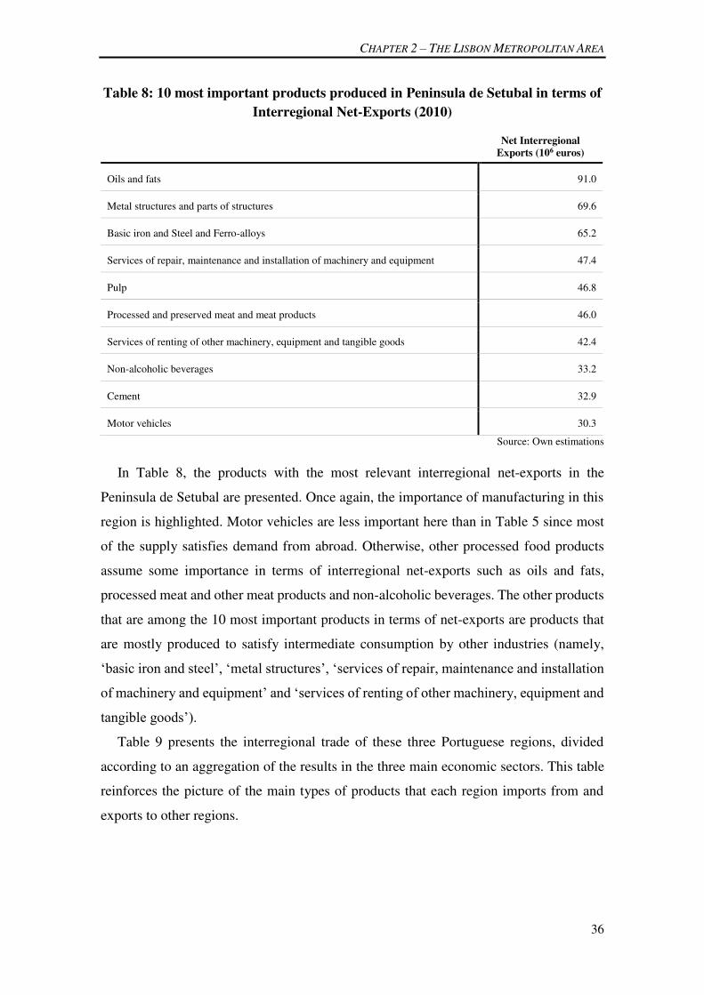
CHAPTER 2 – THE LISBON METROPOLITAN AREA
36
Table 8: 10 most important products produced in Peninsula de Setubal in terms of
Interregional Net-Exports (2010)
Net Interregional Exports (106 euros)
Oils and fats 91.0
Metal structures and parts of structures 69.6
Basic iron and Steel and Ferro-alloys 65.2
Services of repair, maintenance and installation of machinery and equipment 47.4
Pulp 46.8
Processed and preserved meat and meat products 46.0
Services of renting of other machinery, equipment and tangible goods 42.4
Non-alcoholic beverages 33.2
Cement 32.9
Motor vehicles 30.3
Source: Own estimations
In Table 8, the products with the most relevant interregional net-exports in the
Peninsula de Setubal are presented. Once again, the importance of manufacturing in this
region is highlighted. Motor vehicles are less important here than in Table 5 since most
of the supply satisfies demand from abroad. Otherwise, other processed food products
assume some importance in terms of interregional net-exports such as oils and fats,
processed meat and other meat products and non-alcoholic beverages. The other products
that are among the 10 most important products in terms of net-exports are products that
are mostly produced to satisfy intermediate consumption by other industries (namely,
‘basic iron and steel’, ‘metal structures’, ‘services of repair, maintenance and installation
of machinery and equipment’ and ‘services of renting of other machinery, equipment and
tangible goods’).
Table 9 presents the interregional trade of these three Portuguese regions, divided
according to an aggregation of the results in the three main economic sectors. This table
reinforces the picture of the main types of products that each region imports from and
exports to other regions.

CHAPTER 2 – THE LISBON METROPOLITAN AREA
37
Table 9: Overall Interregional Gross and Net exports (106 € and % of regional
GDP) from Greater Lisbon, Peninsula de Setubal and Rest of the Country (2010)
Products Greater Lisbon Peninsula de Setubal Rest of the Country
Gross Exports Net Exports Gross Exp. Net Exports Gross Exp. Net Exports
106 € % 106 € % 106 € % 106 € % 106 € % 106 € %
Primary 103 0 - 910 - 2 167 2 - 206 - 2 1,273 1 1,116 1
Secondary 7,117 12 - 1,785 - 3 2,673 27 - 596 - 6 10,623 10 2,382 2
Tertiary 16,548 29 11,026 19 2,160 21 - 2,146 - 21 5,127 5 - 8,881 - 8
TOTAL 23,767 41 8,332 15 5,001 50 - 2,948 - 29 17,023 15 - 5,385 - 5
Source: Own estimations
From these figures on interregional trade, one can see that although the Greater Lisbon
region has a trade balance surplus regarding the services produced, it faces a deficit
regarding primary goods as well as secondary products (namely some manufacturing and
electricity production). However, as observed previously, the surplus observed for tertiary
products overcomes the deficit obtained in primary and secondary products. In contrast,
the Rest of the Country is the region that mostly exports products associated with the
Primary and Secondary sectors. Despite this, the overall trade balance of the Peninsula de
Setubal presents a large deficit that accounts for almost 30% of its GDP.
These deficits only account for the interregional trade of products, but they can be
offset by other flows. However, as it is possible to observe in Table 4 this is not
compensated for either by international trade or by non-residents in Portugal’s
consumption. So, once again, commuting arises as the most suitable explanation for the
counterpart for this huge deficit.21 Indeed, due to commuting, thousands of households
that live in the Peninsula de Setubal have their monthly salaries paid by the industries
located in the Greater Lisbon region and “transport” that money to the Peninsula de
Setubal region, financing the acquisition of goods and services in this region (which in
many cases have also been imported from other regions or abroad).
2.4. Commuting activity in Portugal and in the LMA
The analysis of the commuting data among the Portuguese regions allows us to
understand the peculiarity of this phenomenon in the LMA. Every decade, the most
relevant data regarding commuting in Portugal is released in the Portuguese Population
Census Publication, produced by the National Statistical Institute (INE). According to the
21 Other common explanations found in the literature are not applicable to the Peninsula de Setubal region:
e.g. a significant amount of government transfers, social security payments, and immigrants' money
transfers to their region of origin.

CHAPTER 2 – THE LISBON METROPOLITAN AREA
38
2011 Census, there were about 4,361,187 Portuguese workers with different commuting
patterns. Table 10 represents the distribution of commuting patterns among Portuguese
workers. Commuting students are excluded from these numbers and from the analysis in
this research project.
Table 10: Commuting Patterns among Portuguese employed resident population
(2011)
Commuting patterns of Portuguese workers Nº %
Work and live in the same municipality 2,860,521 65.6%
Work at home 152,291 3.5%
Work and live in the same “freguesia” 1,242,977 28.5%
Work in a different “freguesia” 1,465,253 33.6%
Work in another municipality 1,429,867 32.8%
Live in Portugal and work in Spain 69,309 1.6%
TOTAL 4,361,187 100%
Source: 2011 Portuguese Census (INE, 2012c)
According to Table 10, most Portuguese workers (more than 65%) live in the same
municipality in which they work, while an important share (around 33%) commutes daily
to other municipalities in order to work. A residual share of less than 2% of Portuguese
workers stated that they commute to Spain in order to work.22 Out of those who work and
live in the same municipality, 5% affirmed that they work at home, 43% stated that they
work within the same “freguesia” (a small administrative area that, in some situations,
may be translated as a parish) and 52% indicated that they have to travel to another
“freguesia”. As already mentioned, for the purposes of this work only those that live and
work in a different municipality are considered as commuters, so in the next sub-sections
and chapters the remaining analysis will focus on commuting between municipalities and
not on movements within or between “freguesias”.
Compared with the 2001 Portuguese Census (INE, 2003), the number of commuters
slightly declined in absolute terms (less 20.000). However, the same happened with total
employment such that the share of workers that traveled daily to other municipalities to
work increased by more than 2%. This comparison demonstrates that commuting is a
“steady” phenomenon in the Portuguese territory that has arisen and become relatively
more important in the last decades.
The Portuguese workers who commute are not distributed homogenously throughout
the Portuguese territory. Table 11 demonstrates the relationship between commuter and
22 Those workers are excluded from the remaining analysis since the goal of this work is focused on the
commuting phenomenon in the LMA and this region has no border with Spain.

CHAPTER 2 – THE LISBON METROPOLITAN AREA
39
non-commuter workers (to different municipalities), by place of residence, in the
Portuguese NUT III regions. Remark that a significant part of these commuters, commute
within the NUTS III where they inhabit, as they live and work in different municipalities.
Indeed, only a small share of workers commute to a different NUTS III. The dichotomy
of commuting “within” and “between” NUTS III persists all over this work.
Table 11: Distribution of commuters and non-commuters, by place of residence,
among the Portuguese NUTS III regions (2011)
Non-commuters Commuters
Workers Nº % Nº %
Portugal 4,290,388 2,860,521 67.2% 1,429,867 32.8%
Minho-Lima 88,240 69,686 79.0% 18,554 21.0%
Cávado 172,626 133,042 77.1% 39,584 22.9%
Ave 214,168 159,745 74.6% 54,423 25.4%
Grande Porto 523,950 296,335 56.6% 227,615 43.4%
Tâmega 208,769 148,693 71.2% 60,076 28.8%
Entre Douro e Vouga 118,650 82,825 69.8% 35,825 30.2%
Douro 72,502 59,000 81.4% 13,502 18.6%
Alto Trás-os-Montes 67,065 58,694 87.5% 8,371 12.5%
Baixo Vouga 166,449 114,005 68.5% 52,444 31.5%
Baixo Mondego 137,150 98,554 71.9% 38,596 28.1%
Pinhal Litoral 111,517 86,426 77.5% 25,091 22.5%
Pinhal Interior Norte 47,904 33,118 69.1% 14,786 30.9%
Dão-Lafões 102,344 78,835 77.0% 23,509 23.0%
Pinhal Interior Sul 13,211 10,738 81.3% 2,473 18.7%
Serra da Estrela 14,559 11,498 79.0% 3,061 21.0%
Beira Interior Norte 37,122 31,257 84.2% 5,865 15.8%
Beira Interior Sul 27,594 24,344 88.2% 3,250 11.8%
Cova da Beira 32,333 26,407 81.7% 5,926 18.3%
Oeste 150,007 105,527 70.3% 44,480 29.7%
Médio Tejo 85,330 59,966 70.3% 25,364 29.7%
Grande Lisboa (Greater Lisbon) 888,557 484,396 54.5% 404,161 45.5%
Península de Setubal 321,263 155,365 48.4% 165,898 51.6%
Alentejo Litoral 38,654 31,614 81.8% 7,040 18.2%
Alto Alentejo 47,557 34,854 73.3% 12,703 26.7%
Alentejo Central 77,239 53,854 69.7% 23,385 30.3%
Baixo Alentejo 52,100 38,409 73.7% 13,691 26.3%
Lezíria do Tejo 91,196 67,362 73.9% 23,834 26.1%
Algarve 184,381 142,595 77.3% 41,786 22.7%
R. A. Açores 101,808 86,947 85.4% 14,861 14.6%
R. A. Madeira 107,637 76,430 71.0% 31,207 29.0%
Source: Own calculations based on 2011 Portuguese Census
As Table 11 highlights, there are only 3 NUT III regions where commuting is more
intensive than the Portuguese average - Peninsula de Setubal, Greater Lisbon and Grande

CHAPTER 2 – THE LISBON METROPOLITAN AREA
40
Porto. These regions account for more than 55% of Portuguese commuters, and the
Lisbon Metropolitan Area is the place of residence for more than 40% of Portuguese
commuters.
Figure 2, which depicts the proportion of commuters in the employed resident
population, at the municipal level, allows us to geographically identify the municipalities
of residence where the commuting flows are more intensive in the Portuguese mainland
territory.
Figure 2: Share of commuters in the employed resident population, by
municipality (2011)
Once more, Figure 2 highlights the relevance of the Lisbon Metropolitan Area,
although it is possible to see that in some municipalities of the Oporto Metropolitan Area
and in the Coimbra region there also exists a relevant intensity of commuting. In the rest
of the municipalities, the relative number of commuters in each municipality is less
relevant (i.e., in most of the municipalities there are less of 15 commuters per 100
employed inhabitants).

CHAPTER 2 – THE LISBON METROPOLITAN AREA
41
The commuting activities happen mainly among neighboring municipalities located
within the same administrative region. In Portugal, an average of 11.5% of workers travel
daily to other NUT III regions while 32.8% travel to a different municipality. However,
there are commuting activities among some Portuguese NUTS III regions, namely
affecting the Greater Lisbon region. Table 12 presents the top 5 most intensive
interactions between different NUT III regions of workers by place of residence.
Table 12: Share of workers, by place of residence, which commute to other NUT
III region (2011)
Place of Residence NUT III Working Place NUT III % of working residents travelling
between the 2 NUTS III
Peninsula de Setubal Greater Lisbon 30.8%
Pinhal Interior Norte Baixo Mondego 15.7%
Oeste Greater Lisbon 12.9%
Leziria do Tejo Greater Lisbon 11.2%
Tâmega Grande Porto 9.2%
Source: Own calculations (based on 2011 Portuguese Census)
Table 12 highlights the critical capacity of the Greater Lisbon region to attract workers
that live in other regions. Indeed, Greater Lisbon can attract more than 10% of workers
living in the regions of Peninsula de Setubal, Oeste and Leziria do Tejo. Once more, the
analysis of the commuting data underlines the relevance of commuting between the
Greater Lisbon region and its surroundings (particularly the Peninsula de Setubal region).
However, despite the importance of the Greater Lisbon NUTS III region as an important
employment center for the population of the neighboring regions, commuting is relatively
more relevant among the workers who live within this region.
The description of the commuting flows proves the relevance of this activity in the
Lisbon Metropolitan Area. Table 13 details the origin-destiny of Portuguese workers with
a special focus on those who work or live within the Lisbon Metropolitan area, comprising
the two NUTS III regions.
Table 13: Portuguese workers origin-destiny matrix (2011)
Workplace
Residence
Location
Same municipality
(non-commuters)
Other municipalities (commuters)
Greater Lisbon Peninsula
Setubal
Rest of the
Country
Greater Lisbon 484,396 370,776 13,633 13,044
Peninsula Setubal 155,365 98,762 60,521 4,048
Rest of the Country 2,220,760 36,138 3,855 829,090
Source: Own calculations (based on 2011 Portuguese Census)
CHAPTER 2 – THE LISBON METROPOLITAN AREA
42
According to Table 13, around 45% of those who work and live in the Lisbon
Metropolitan area are commuters. Among those living in the Greater Lisbon NUT III
region, 55% are non-commuters, 42% travel between municipalities located within the
Greater Lisbon NUT III region and 3% travel to the Peninsula de Setubal or to the Rest
of the Country to work. In the Peninsula de Setubal, 48% of its employed or self-
employed inhabitants are non-commuters, 19% travel between municipalities located
within the Peninsula de Setubal NUT III region and more than 30% travel to the Greater
Lisbon NUT III region in order to work. So, in the case of Greater Lisbon, the commuting
flows are more intense among the municipalities located within the NUT III region.
However, the commuting of Peninsula de Setubal residents to work in Greater Lisbon
corresponds to a high share of total employed inhabitants in that region and represents the
most intensive commuting flow concerning the Portuguese NUTS III regions.
Indeed, among the Portuguese municipalities, those located in the Lisbon Metropolitan
Area rank among those with a higher relative share of commuters, well above the
Portuguese average number of commuters. Table 14 presents some indicators regarding
commuting among the Lisbon Metropolitan Area municipalities.

CHAPTER 2 – THE LISBON METROPOLITAN AREA
43
Table 14: LMA demographic indicators, employment and share of commuters by
municipality (2011)
Municipality
Total
Population (1)
Employed
population living in the municipality
(2)
Employed persons
working in the municipality
(3)
Out-commuters
as % of employed
population (4)
Workers in the municipality /
Employed population
(3) / (2)
Amadora 175,558 72,995 51,817 64% 71%
Cascais 205,117 88,656 67,995 45% 77%
Lisboa 545,245 226,622 531,214 17% 234%
Loures 205,577 89,056 68,638 57% 77%
Mafra 76,749 35,603 25,630 44% 72%
Odivelas 143,755 66,107 32,998 65% 50%
Oeiras 172,063 75,820 84,914 56% 112%
Sintra 377,249 168,447 108,673 52% 65%
Vila Fr. Xira 136,510 64,943 42,420 54% 65%
Alcochete 17,565 7,928 7,042 59% 89%
Almada 173,298 70,012 54,293 51% 78%
Barreiro 79,042 30,544 20,800 57% 68%
Moita 66,311 25,439 12,806 63% 50%
Montijo 51,308 22,637 18,486 48% 82%
Palmela 62,549 26,410 27,371 48% 104%
Seixal 157,981 67,887 36,205 60% 53%
Sesimbra 49,183 21,570 13,164 50% 61%
Setúbal 120,791 48,711 45,999 31% 94%
TOTAL 2,815,851 1,209,387 1,250,465 103%
Source: Own calculations (based on 2011 Portuguese Census)
Table 14 reinforces the commuting relevance in the Lisbon Metropolitan Area. Indeed,
only the Lisbon and Setubal municipalities reveal a relatively small share of commuters
among their inhabitants. Odivelas, Amadora and Moita have the most intense outgoing
commuting activity regarding their employed resident population, with more than 60%
of their resident workers traveling to other municipalities in order to work. In contrast,
only 2 municipalities have a lower share of commuters than the Portuguese average
(Lisbon and Setubal). In the case of Setubal, this is because this municipality was the
head of a former administrative territorial division (Distrito) and therefore some relatively
important services are still located there, which refrain the outgoing commuting flows.
This is also the reason for the small difference, in Setubal municipality, between
employment positions and the employed population living in this municipality. Other
municipalities, as Oeiras or Palmela, also have more employment positions than the
working population living in the municipality. There are various reasons for this. Due to
its geographical proximity to Lisbon, Oeiras has become an important employment center

CHAPTER 2 – THE LISBON METROPOLITAN AREA
44
with many firms opting to locate their headquarters in this specific municipality.
Furthermore, Palmela is capable of attracting an important share of workers from the
neighboring municipalities since one of the most important Portuguese manufacturing
plants is located there (Autoeuropa, dedicated to the manufacturing of cars and other
vehicles). Figure 3 illustrates, using Geographical Information Systems, the most
important commuting flows in the Lisbon Metropolitan Area. Red border defines the
Greater Lisbon NUTIII region and blue border defines the Peninsula de Setubal region.
Figure 3: Commuting flows in the Lisbon Metropolitan Area (2011)
Figure 3 demonstrates the central importance of the Lisbon municipality (with several
incoming flows of more than 25 thousand people) while also highlights the existence of
some important flows of commuting between other municipalities. But, despite these
second-order central places, the case of the Lisbon municipality, the Portuguese Capital,
is the most paradigmatic one in Portugal. It is the most important employment center in

CHAPTER 2 – THE LISBON METROPOLITAN AREA
45
Portugal and is the municipality that attracts more workers from different municipalities
(in absolute terms and relatively when compared with the number of inhabitants). The
attraction capacity is higher amongst the municipalities adjacent to this municipality but
its influence extends far beyond its borders. Figure 4 demonstrates the share of the
working population that live in a different municipality but work in the Lisbon
municipality.
Figure 4: Share of employed population working in the municipality of Lisbon, by
place of residence (2011)
According to Figure 4, there is a significant number of municipalities in which more
than 15% of their working population travel to the Lisbon municipality in order to work.
Most of these municipalities are located in the Greater Lisbon region. Odivelas is the
municipality from which the most workers travel daily to the Lisbon municipality (more
than 40%). In most of the Lisbon Metropolitan Area municipalities the value is above
30%, including some municipalities located in the Peninsula de Setubal (Almada,
Barreiro, and Seixal).
Since commuters travel between different municipalities, they also have to deal with
different journeys (in distance and time). A commuter who travels daily between Sintra

CHAPTER 2 – THE LISBON METROPOLITAN AREA
46
and Lisbon bears a different “cost” than a commuter who travels between Palmela and
Lisbon. Thus, longer trips have higher externality impacts associated with commuting.
So, combining the commuter origin-destiny matrix (Table 13) with the distance of each
journey (Ferreira et al., 2012), the total amount of kilometers travelled is estimated. This
allows us to estimate a new dimension of the commuting phenomenon within a region.
Table 15 presents the results of the kilometers travelled by commuters within, coming
into or going out of the Lisbon Metropolitan Area.
Table 15: Number of kilometers (103) travelled by commuters per day by the LMA
workers/residents (2011)
Workplace Residence
Greater Lisbon Peninsula Setubal Rest of the Country
Greater Lisbon 17,128 1,031 1,757
Peninsula Setubal 5,848 2,529 794
Rest of the Country 5,076 683 -----
Source: Own calculations
As Table 15 demonstrates, commuters in this region travel almost 35 million
kilometers every day.23 Commuters who work in Greater Lisbon are the most important
share in terms of travelled-distance (more than 80%). Specifically, those who work and
live in the Greater Lisbon region are responsible for almost 50% of the total kilometers
travelled. The average distance (combining going and coming back from work) travelled
by commuters is also different according to the distinct travel-to-work journey patterns.24
Table 16 represents the Lisbon Metropolitan Area commuters’ average travel distance per
day.
Table 16: Daily average kilometers (103) traveled by commuters working or living
in the LMA (2011)
Workplace
Residence Greater Lisbon Peninsula Setubal Rest of the Country
Greater Lisbon 46.2 75.6 135.0
Peninsula Setubal 59.2 41.8 158.0
Rest of the Country 140.5 157.1 -----
Source: Own calculations
23 Based on the 2001 Portuguese Census and on the distance between Portuguese municipalities, Ferreira
et al. (2014a) estimated that 59% of the kilometers traveled by inter-municipality commuters correspond to
trips made inside the Portuguese metropolitan areas of Lisbon and Oporto, confirming the relevance of
these regions to commuting activity in Portugal. 24 According to Ferreira et al. (2014a), in 2001 Portuguese commuters travelled an average distance of
approximately 56 km per day. In 2011, this value increased to an average distance of 64 km per day.

CHAPTER 2 – THE LISBON METROPOLITAN AREA
47
According to Table 16, despite the fact that a large number of commuters are
concentrated in the Greater Lisbon region, those who travel from/to the Rest of the
Country have to bear longer distances in their commuting activity. Those who travel
between Greater Lisbon and the Peninsula de Setubal also account for a larger number of
kilometers than those that just travel within the NUTS III regions.
These results highlight the relevance of the commuting process within and between
the Greater Lisbon and Peninsula de Setubal regions. Additionally, they also show that
despite the important commuting flows among and between these NUTS III regions the
commuting activity related to the LMA also affects residents and jobs in other
neighboring regions.
Another important conclusion that can be drawn from a more detailed observation of
the 2011 Portuguese Census comprises the heterogeneity associated with commuting
intensity by different industries located in different regions. To offer an illustrative
representation concerning the residential location of the Greater Lisbon and Peninsula de
Setubal workers by industry, in Table 17a and 17b, are presented the top 3 industries
attracting more (and less) commuters from the other regions included in the model (as
well as the corresponding average values).
Table 17a: Industries attracting more and less commuters in Greater Lisbon
according with the place of residence of the workers
% of Full-Time Equivalent (FTE) jobs
satisfied by workers that live in
the same municipality
where they work
Total Share of
commuters
other municipalities
within GL
PS RC
Top 3 industries attracting more commuters
Water Transport 29% 71% 39% 25% 7%
Air Transport 29% 71% 49% 15% 7%
Computer programming,
consultancy and related activities 32% 68% 48% 16% 4%
Average Values 49% 51% 37% 10% 4%
Top 3 industries attracting less commuters
Fishing and aquaculture 64% 36% 22% 10% 4%
Manufacture of basic metals 65% 35% 26% 6% 3%
Agriculture, farming of animals,
hunting and related service activities 74% 26% 14% 3% 9%
Source: Own calculations

CHAPTER 2 – THE LISBON METROPOLITAN AREA
48
Table 17b: Industries attracting more and less commuters in Peninsula de Setubal
according with the place of residence of the workers
% of Full-Time Equivalent (FTE) jobs
satisfied by workers that live in
the same municipality
where they work
Total Share of
commuters
other municipalitie
s within PS
GL RC
Top 3 industries attracting more commuters
Manufacture of motor vehicles, parts
and accessories for motor vehicles 32% 68% 61% 5% 2%
Services of renting of other
machinery, equipment and tangible
goods
44% 56% 27% 18% 11%
Scientific research and development 44% 56% 20% 37% 2%
Average Values 67% 33% 26% 6% 2%
Top 3 industries attracting less commuters
Food and beverage service activities 83% 17% 15% 2% 1%
Activities of households as
employers of domestic personnel 88% 12% 10% 2% 1%
Fishing and aquaculture 93% 7% 5% 1% 2%
Source: Own calculations
According to Table 17a, 71% of “Water Transport” industry workers in Greater Lisbon
are commuters. The industry attracting less commuters among its workforce is
“Agriculture, farming of animals, hunting and related service activities” (for which about
¾ of the workers live in their workplace municipality, i.e. do not commute). In average
terms, 37% of Greater Lisbon workers commute to municipalities located within the
region, 10% live in the Peninsula de Setubal region and 4% live in the Rest of the Country
region. Additionally, Table 17b also highlights significant commuting ‘attractiveness’
differences among the industries located in the Peninsula de Setubal region. In this
specific case, the industry with relatively more commuters in its workforce is the
“Manufacture of motor vehicles, parts and accessories for motor vehicles” industry (of
which 68% of the workers are commuters). In contrast, the “Fishing and aquaculture”
industry only embodies 7% of commuters among its workforce.
Commuting is also not homogeneous in terms of the means of transport used in the
journey to work (the modal split). Some workers may travel to their workplace on foot,
while others may use public transportation or travel by car. In Portugal, and in the Lisbon
Metropolitan area, most workers travel by car and the use of public transportation
relatively low compared with other countries of the European Union (Eurostat, 2015).
However, the modal split depends on the distance-travelled between the place of
residence and the workplace. Table 18 represents the modal split in the Lisbon
Metropolitan Area and in the Rest of the Country according to the different travel patterns.

CHAPTER 2 – THE LISBON METROPOLITAN AREA
49
Table 18: Modal split in Lisbon Metropolitan Area and in the Rest of Country
according with the different travel patterns
Travel Pattern Main Transportation Used
On Foot Car
Public Transportation
Other Bus
Train /
Subway Boat
(%) (%) (%) (%) (%) (%)
Lisbon Metropolitan Area
Same freguesia 39.8% 47.5% 9.5% 1.5% 0.0% 1.7%
Other freguesia in the same
municipality 5.8% 61.9% 19.3% 11.2% 0.0% 1.8%
Other municipality 0.7% 60.4% 15.2% 19.8% 2.6% 1.3%
TOTAL 10.1% 58.4% 15.4% 13.4% 1.2% 1.5%
Rest of the Country
Same freguesia 36.2% 55.8% 3.7% 0.1% 0.0% 4.2%
Other freguesia in the same
municipality 5.3% 81.2% 9.8% 0.8% 0.0% 2.8%
Other municipality 0.9% 81.3% 10.9% 5.3% 0.0% 1.6%
TOTAL 14.9% 72.3% 10.1% 1.8% 0.0% 3.0%
Source: 2011 Portuguese Census (INE, 2012c)
As Table 18 reveals, the non-use of motorized vehicles in journeys to work is almost
exclusive to workers who live and work in the same freguesia and is residual among those
who travel among municipalities (either in the Rest of the Country or in the Lisbon
Metropolitan area) and is confined to people living and working near the municipalities
border. In contrast, the use of cars is above average for those who work in a different
freguesia (and municipality) from their place of residence and is relatively more important
in Portugal than in the Lisbon Metropolitan Area. Compared with the Rest of the Country,
the modal split in the Lisbon Metropolitan Area is mostly characterized by a higher use
of public transportation, namely trains, the subway and boat transportation.25 This
happens mostly as a response to two important drivers: first, there are more costs
associated with car use (e.g., congestion, higher parking prices, less accessibility to
parking, tolls); second, in the LMA there is a more extensive (and functional) public
transportation network with urban trains and different bus companies linking several
municipalities. Lastly, one important point regarding the modal split is the use of more
than one means of transportation. In the Rest of the Country, 12.2% said that they usually
use more than one means of transportation when commuting to work. This value is
25 Boat transportation in the Lisbon region concerns those crossing the Tagus River connecting the NUTS
III regions. The remaining commuters in Portugal – in fact a residue - which use boat transportation for
commuting purposes are located in the Azores – mainly between Faial and Pico Islands - or in the Aveiro
municipality.

CHAPTER 2 – THE LISBON METROPOLITAN AREA
50
significantly higher in the Lisbon Metropolitan Area where almost 25% of the workers
stated that they use more than one type of transportation. The number is also significantly
higher among those who travel daily to another municipality (31%). The number of
workers who use more than one means of transport reveal the importance of multi-modal
passenger transportation in the Lisbon Metropolitan Area in comparison with the Rest of
the Country.
Finally, commuting activity imposes a burden on commuters in terms of the time spent
on their journey to work. Thus, the intense commuting observed in the Lisbon
Metropolitan Area is also reflected in the average time spent by workers on their journey
to work. According with 2011 Portuguese Census, Table 19 compares the average time
spent by workers every day according with the type of transportation used.
Table 19: Average time spent (in minutes) on commuting by means of transport
and by region of residence (2011)
By car
By public
transportation Total
Lisbon Metropolitan Area 22.1 42.5 26.4
Greater Lisbon 21.8 40.7 25.8
Peninsula de Setubal 22.9 47.7 28.0
Portugal 18.0 34.3 20.0
Source: 2011 Portuguese Census (INE, 2012c)
Table 19 highlights that commuting is more time-consuming in the Lisbon
Metropolitan Area in comparison with the Portugal average. Indeed, in average terms, a
commuter in the Lisbon Metropolitan Area spends 32% more time than the average
Portuguese commuter. This difference is smaller, but still relevant, when compared with
public transportation commuters (23% more time consumed by Lisbon residents) and car
users (more 22%).26 Indeed, both NUTS III regions comprising the Lisbon Metropolitan
Area have higher values of average commuting time duration among the 30 Portuguese
NUTS III regions, independently of the travel mode used.
2.5. Final Comments
This chapter started by exploring some economic indicators regarding the LMA. It was
possible to observe that the LMA region is a very ‘open’ region that produces several
26 The higher gap for commuters as a whole, compared with the analysis by means of transport, mirrors a
structure effect. The average time spent by an LMA commuter is basically higher, compared with the
Portuguese average, because more people use public transportation and less use their own car.

CHAPTER 2 – THE LISBON METROPOLITAN AREA
51
services and manufactures products for the ‘Rest of the Country’ as well as others to be
exported internationally. Using more disaggregated information, it was made clear that
an important share of the manufacturing industries is located in the Peninsula de Setubal
but almost all services (except those that must be locally provided) are located in the
Greater Lisbon region (and, very likely in the Lisbon municipality and in its proximities).
Many of these services’ exports correspond to “headquarter services” provided by firms
headquarters, located in this region, to the different establishments located sparsely all
over the country. According to the National Accounts rules, this kind of service is
considered to be an ancillary activity and so is allocated to the main scope of the firm.27
That is to say, there is not accounted a specific industry to headquarters. For this reason,
the headquarters services emerge as exports of wholesale trade, financial or insurance
products, human health services, electricity distribution, gas distribution and provision,
and so on.
As the LMA concentrates a thrilling agglomeration of people and jobs and an
important variety of economic activities, this actually contributes to potentiating the
existence of commuting, which, as was shown, assumes a relatively large proportion in
this region when compared to the ‘Rest of the Country’. This influences the intensity of
commuting but also has other important consequences in terms of the modal split, number
of kilometers travelled, time spent commuting and the different ‘commuter attractiveness’
of the industries located in the two regions.
27 According to the UN (2008: 68), these types of activities are described as including the overseeing and
managing of other units of the company or enterprise; undertaking the strategic or organizational planning
and decision making role of the company or enterprise; and exercising operational control and manage the
day-to-day operations of their related units. Moreover, such units are allocated to the non-financial
corporations sector unless all or most of their subsidiaries are financial corporations, in which case they are
treated by convention as financial auxiliaries in the financial corporations sector.

How will the cessation of war purchases … affect the national level of employment? How many new jobs will be
created by the consumers’demand for an additional one million of passenger cars, how many of these jobs can be
expected to be located in the automobile industry itself, and how many
in other industries such as Steel and the Chemicals,
the Coal and the Petroleum industries?
W. Leontief, 1941
CHAPTER 3 – MULTI-REGIONAL INPUT-OUTPUT
MODELS
3.1. Introduction
Multi-Regional Input-Output (MRIO) models represent a relevant advance regarding
the former and most frequently applied single-region Input-Output (I-O) models. Indeed,
MRIO models improve the recognition, in an operational way, of the interdependencies
established between economic agents located in different regions (Miller and Blair, 2009:
76). As commuting prevails in urban areas, it also contributes to intensifying the
interdependencies among industries and households located in different regions of a
certain metropolitan region. Thus, an MRIO modeling framework may constitute a
suitable approach to assessing the impacts that stem from this particular phenomenon. On
the other hand, MRIO models usually demand a significant amount of data that is not
directly available from National Statistical Offices.
This chapter is devoted to discussing the different steps in estimating the data that
supported the development of the MRIO model applied to the Lisbon Metropolitan Area
(LMA). This ongoing “journey”, involving mainly researchers of the University of
Coimbra, started in 2010. The author of this dissertation was privileged to participate

CHAPTER 3 – MULTI-REGIONAL INPUT-OUTPUT MODELS
54
from the very beginning of this challenge and actively contributed as a researcher in every
step of this collective construction. . Indeed, the estimation of the first consistent set of
I-O regional tables for all the NUTS III Portuguese regions, had its impulse in the scope
of DEMOSPIN (Economically Sustainable DEMOgraphy - ReverSing the Decline in
Peripheral RegIoNs), a research project funded by the Portuguese Foundation for Science
and Technology (PTDC/CS-DEM/100530/2008). This project emerged for the purpose
of bridging two scientific areas (economics and demography) and had the ambition of
studying how the ageing process and the economic decline could be reversed in the
Portuguese peripheral regions. For this purpose, 14 matrices were built, for 2007, one for
each focus region. These were single-region models that described, with a relevant level
of disaggregation (431 products and 125 industries), the intra-regional flows in each of
these regions. One important limitation of single-region I-O models is that they fail to
include the full specification of interregional trade. Their most important limitation
therefore consists of ignoring trade linkages between regions. In fact, if for example, a
region suffers a hypothetical shock, some of the inputs needed to ‘deal with’ the impact
in production come from the remaining regions – spillover effects. The production in
those regions may also need to import inputs from other regions (including the one that
suffered the initial shock). These effects concern the concept of interregional feedback
effects. These kinds of spatial linkages are precisely what distinguishes complete
interregional from single-region models (Miller and Blair, 2009: 81)
This specific limitation of the derived regional I-O tables has been overcome, in the
context of the following research project, EMSURE (Energy and Mobility for
SUstainable Regions, framed under the Energy for Sustainability Initiative of the
University of Coimbra and funded by MaisCentro – an operational program in the
Portuguese Centro Region funded by the European Union - and the Portuguese
Foundation for Science and Technology (CENTRO-07-0224-FEDER-002004). In this
case, our specific research objective consisted of deriving a bi-regional model – for the
Portuguese NUT II Centro Region and the ‘Rest of the Country’ – and compiling an
extensive statistical database on economy, energy and environment with the aim of
generating the required satellite accounts for the NUT II Centro Region. The same
approach was also used for other geographic configurations of bi-regional type (e.g. Coast
versus Interior of Portugal) addressing other specific purposes. Thus, together with the
aim of fulfilling the EMSURE objectives, there was the ambition of compiling a broader
database with the goal of amplifying the potential scope of our work. This was the origin

CHAPTER 3 – MULTI-REGIONAL INPUT-OUTPUT MODELS
55
of what is hereafter designated the MULTI2C database, a general flexible approach,
developed mainly in the University of Coimbra, which allows for the construction of
MRIO models for different geographic configurations and empirical applications (aimed
at Portuguese regional economies).
Such a process implied different types of frameworks and several research issues were
studied in the scope of DEMOSPIN and EMSURE (Barata et al., 2013; Ramos et al, 2013;
Ramos et al., 2015). This chapter is specifically devoted to the methodology used in the
development of the MRIO framework applied to the LMA. This application has a feature
that makes it distinctive from other MULTI2C models: it abandons the bi-regional
constraint and aims to build up a tri-regional model. Accordingly, this chapter provides
an explanation of the methodology followed. The next section starts by presenting an
overview of the characteristics and procedures applied to formatting the MULTI2C data
at national level. Next, the process of regionalizing the I-O tables is addressed, namely
exploring the interregional trade in the context of bi-regional I-O models. Finally, one of
the main characteristic of this thesis frame is presented, namely by exploring the methods
applied to derive a tri-regional I-O model for the LMA.
3.2. MULTI2C – Shaping a Portuguese National Matrix for
Impact Assessment
The starting point for deriving the information incorporated in the MULTI2C database
(in its most recent version for the year 2010) was the National Accounts (ESA, 1995; base
2006) produced by the National Statistical Institute (INE). From this source, the following
were specifically used:
• The Supply and Use Table (with one single column as the origin of the
domestic product supplies and including basic information on the
decomposition of the industries GVA);
• The Production Matrix - industries that produce the products as primary or
secondary products;
• Employment – individuals and full-time equivalent workers by industry.
The Supply and Use Table and the Production matrix have a significant level of detail
concerning both the number of products (431) and the number of industries (125) that
produce and use them. This framework is also commonly designated as the ‘rectangular’
approach (or the “non-square” I-O frame). In this framework, two dimensions are

CHAPTER 3 – MULTI-REGIONAL INPUT-OUTPUT MODELS
56
simultaneously considered (products and industries): the Use table, which describes the
consumption of products by the several industries, and the Production Matrix, which
represents the distribution of the industries’ output by product. According to the System
of National Accounts (SNA) (UN, 2008: 18), the term product is a synonym of goods and
services, which are always a result of production, either domestically or abroad, in a
certain period of time. Additionally, an industry consists of a group of establishments
engaged in the same, or similar, kinds of activity (UN, 2008: 87).
In the particular case of the Portuguese Supply and Use Table in its original form, the
information that is available is at purchasers’ prices and total flows. This means that the
cells in the Intermediate Consumption and Final Demand Matrices also account for
different Taxes and Subsidies (e.g., VAT and Other Taxes and Subsidies on Products)
borne by the different flows. The trade and transport margins are also allocated to the
traded and transported products not to their specific industries. On the other hand, those
matrices also include the inputs supplied from abroad. The available data was assembled
according to Figure 5.
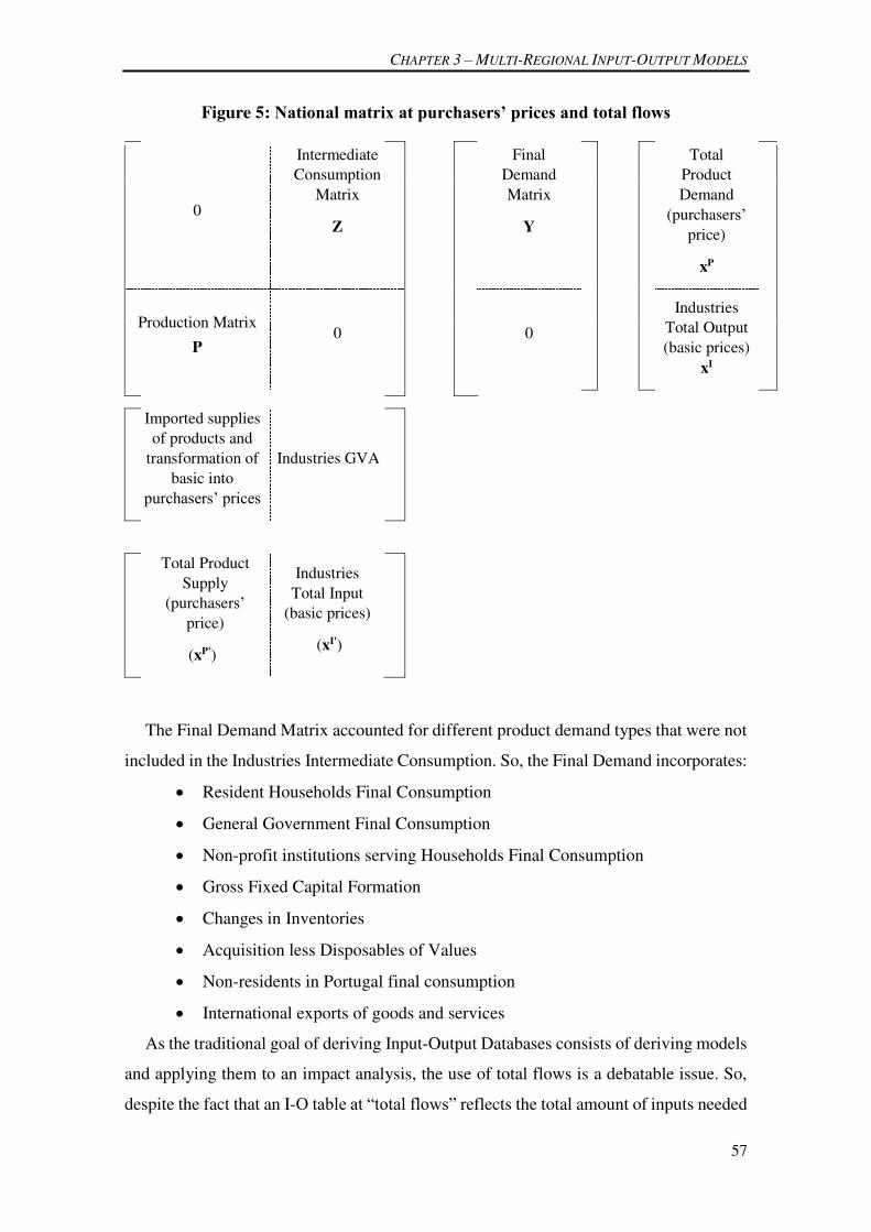
CHAPTER 3 – MULTI-REGIONAL INPUT-OUTPUT MODELS
57
Figure 5: National matrix at purchasers’ prices and total flows
0
Intermediate Consumption
Matrix
Z
Final Demand Matrix
Y
Total Product Demand
(purchasers’ price)
xP
Production Matrix
P 0
0
Industries
Total Output (basic prices)
xI
Imported supplies
of products and transformation of
basic into purchasers’ prices
Industries GVA
Total Product Supply
(purchasers’ price)
(xP')
Industries Total Input
(basic prices)
(xI')
The Final Demand Matrix accounted for different product demand types that were not
included in the Industries Intermediate Consumption. So, the Final Demand incorporates:
Resident Households Final Consumption
General Government Final Consumption
Non-profit institutions serving Households Final Consumption
Gross Fixed Capital Formation
Changes in Inventories
Acquisition less Disposables of Values
Non-residents in Portugal final consumption
International exports of goods and services
As the traditional goal of deriving Input-Output Databases consists of deriving models
and applying them to an impact analysis, the use of total flows is a debatable issue. So,
despite the fact that an I-O table at “total flows” reflects the total amount of inputs needed

CHAPTER 3 – MULTI-REGIONAL INPUT-OUTPUT MODELS
58
by domestic producers, some of the demand shocks measured by the model will be felt
internationally (Miller and Blair, 2009: 30). The same concern arises regarding Taxes and
Subsidies and the transformation from “purchaser prices” to “basic prices”. According to
the UN (2008: 102), “purchaser prices” is the amount paid by the buyer for a unit of
output less any taxes invoiced by the seller but deductible by the purchaser. It should be
equal to the basic price plus non-deductible taxes on products less subsidies on products
and it incorporates the transport costs and trade margins on products, which are not
separately invoiced. Thus, the part of the monetary flows among industries,
corresponding to taxes, subsidies, benefits, and trade and transportation margins is not set
apart when the I-O matrix is at “purchaser prices”. Thus, a bunch of transformations were
needed in order to better suit data to impact analysis applications.
Another important transformation was also performed in setting the national frame of
the MULTI2C models. The original information provided by the Portuguese National
Accounts Supply and Use Tables (INE, 2012a) only considered one aggregated industry
describing the inputs and outputs of electricity production and distribution (“351 -
Production, transmission, distribution and trade of electricity”). One of the first
transformations made consisted of disaggregating this particular sector. There were three
different reasons for choosing this option: first, the relevant differences between
production and distribution technology (and consequently the respective use of inputs);
second, the differences in the inputs used by the different technologies for producing
electricity; and thirdly, the aim of simulating the different environmental impacts that
could result from the use of different sources of electricity production. Therefore, the
procedure consisted in splitting the total production and intermediate consumption of the
National Accounts electrical sector by one industry of electricity distribution and 9
industries of electricity production according to the following sources: 1) wind; 2)
geothermal; 3) hydro; 4) photovoltaic; 5) coal; 6) fuel oil; 7) natural gas; 8) diesel; and 9)
cogeneration. Each of these “new industries” included in the model have a new (and
specific) production technology and different Outputs, GVAs and Intermediate
Consumption. The procedure applied in this partition is detailed in Ramos et al. (2015).
At this point the model was extended, keeping its “rectangular format” and still
comprising 431 products, but now having 134 industries (instead of the 125 considered
in the National Accounts).

CHAPTER 3 – MULTI-REGIONAL INPUT-OUTPUT MODELS
59
3.2.1. From purchaser to basic prices
The first step in transforming Figure 5, in order to get a more operative scheme, was
to adapt it to basic prices. This specific treatment was performed in three different steps.
First, the VAT included in each product specific use was estimated. Next, a similar
estimation was made regarding the Other Taxes less Subsidies on products. Finally, the
trade and transport margins were estimated and incorporated in a specific part of the
framework and treated as the production of particular products in the economy.
To estimate the VAT affecting different product uses a VAT matrix was estimated
departing from the information obtained from the National Statistical Institute.28 Non-
deductible VAT is supported by both industries and households; however households
final consumption supports a VAT average tax rate that is much higher than that
supported by industries. The idea is that households, as a rule, cannot deduct the VAT
they bear, while the opposite happens for industries (which, as a rule – with a few
exceptions – have the prerogative to deduct into the VAT they pay the one they bear in
the inputs they buy). Therefore, the actual knowledge of the VAT matrix had an important
role in improving the estimation quality. The value of each cell, in matrices Z and Y of
Figure 5, was reduced by amount of the non-deductible VAT actually supported by each
product in each use, generating new matrices expunged from VAT. The VAT supported
by the industries in their purchases was dragged down to a row (below the Intermediate
Consumption Matrix) to keep constant the Industries Total Input. A similar process was
also applied in the case of the Final Demand Matrix, generating a new row detached from
the former matrix (see Figure 6 ahead).
Next, a similar procedure was applied to expunge Other Taxes and Subsidies on
Products from the Intermediate Consumption and Final Demand Matrices. The main
difference was the lack of appropriate official information, capable of separating the
taxes, less subsidies supported by each product, according to the different destinations.
On the other hand, a deductibility mechanism of the VAT kind does not exist for these
taxes, such that the exemption according to the destination is the exception and not the
rule. So, a matrix of Other Taxes and Subsidies supported by products was estimated
assuming the principle of an identical tax rate for each product consumption (with a few
28 In fact, this information was only available to 2007 but it was updated to 2010.

CHAPTER 3 – MULTI-REGIONAL INPUT-OUTPUT MODELS
60
exceptions, which were the same for all uses).29 Once again, the cells of the Intermediate
Consumption and Final Demand matrices were expunged from the estimated value and
the corresponding value was added in the rows inserted below those matrices (see Figure
6).
The last transformation regarded the treatment of the Trade and Transportation
Margins.30 In National Accounts Supply and Use Tables, the total trade and transport
margins columns always add up to zero. This happens because the margins’ value is
reallocated from the industries that generate them, to be incorporated in the purchasers’
price of the products upon which they fall. Thus, while most of the products support the
“payment” of these margins, there are other products (those included in Tables 20 and
21) that “benefit” from them. In the process of transforming the matrices to “basic prices”
these margins are considered to be products of the industries that generate them: the trade
and transportation services themselves. The amount of margins that are supported or
benefit each of the products considered in the model was found from the National
Accounts Supply and Use Table.
According to the level of disaggregation, the trade margins may be seen as four
products of the typical trade industries, namely those depicted in Table 20.
Table 20: Products yielding to Trade margins
4501 Wholesale and retail trade services and repair of motor vehicles and motorcycles
4602 Wholesale trade services (include commission trade), except of motor vehicles and motorcycles
4701 Retail trade services, except of motor vehicles and motorcycles and except fuel in specialized stores
4702 Retail sale of automotive fuel in specialized stores
Each trade margin borne by the different products’ destination was allocated
specifically to each one of the products in Table 20.31 At this point, the sum of the rows
of the Intermediate Consumption plus Final Demand Matrix, associated with these four
products, equals, at basic prices, the product production (at basic prices) declared in the
29 In this distribution, it is considered that the uses associated with changes in inventories and international
exports did not, as a rule, support taxes less subsidies. In the case of some specific financial and insurance related products, it was considered that exports also bear taxes, according to the study by Dias (2008).
30 According to the UN (2008: 102) the margin represents the difference between the price paid by the final purchaser of a product after it has passed through the commercial and transportation chains and the basic price received by its producer.
31 E.g., the product “Wholesale and retail trade and repair of motor vehicles and motorcycles” exclusively embedded the margins supported by products associated with vehicles and motorcycles. Additionally, the retail trade margins were mostly supported by household final consumption while the wholesale trade margins were divided by the Final and Intermediate uses.

CHAPTER 3 – MULTI-REGIONAL INPUT-OUTPUT MODELS
61
Production Matrix. This rule also applies to the other products, since the total value of
their consumption was now reduced according to the supported trade margins.
An identical procedure was applied to estimate and re-direct the incorporated value of
the transportation margins in each product use. According to the National Accounts, the
transportation margins are considered to proceed from the following products, presented
in Table 21.
Table 21: Products yielding to Transportation margins
49012 Freight transport via railways
4903 Freight transport by road and removal services.
5003 Sea, coastal and inland freight water transport
At this point these trade and transportation margins are products by themselves and do
not add up to the value of other products. The Intermediate Consumption matrix describes
the interactions among products and industries in the Portuguese economy, at basic prices,
as defined by the System of National Accounts (UN, 2008: 101): “the amount receivable
by the producer from the purchasers for a unit of output. Thus, it should exclude any tax
assessed on the output (i.e., taxes on products) and include any subsidies on the output
that the producer receives. It also excludes any transport charges invoiced separately by
the producer”. Furthermore, as the SNA explicitly defines, if the product supports trade
margins, it is also necessary to exclude this value from the basic prices (UN, 2008: 103).
This transformation was also included. The Final Demand matrix is, likewise, at basic
prices.
3.2.2. From total to domestic flows
The next step consisted of “transforming” the Intermediate Consumption and Final
Demand Matrices from total to domestic flows. This is fundamental in order that the
database conforms to the impact analysis. An international import matrix was estimated,
departing from the international imports by product from the Portuguese National
Accounts. This was made considering the same propensity to import despite the use
associated with each product (other industry or the different final demand components).32
32 The exception was for international exports, where it was assumed that they were not fed by
international imports, without any national transformation and added value (following Lahr, 2001). The exceptions were the (very rare) products in which the international imports account for, at least, more than 98% of the total supply. This is a reasonable assumption for a non-hub economy such as Portugal.

CHAPTER 3 – MULTI-REGIONAL INPUT-OUTPUT MODELS
62
Using a procedure similar to that used for taxes less subsidies, international imports were
dragged down from matrices Z and Y to row vectors in the bottom part of the table, as
shown in Figure 6.
At this point, the National matrix had the design presented in Figure 6.
Figure 6: National matrix at “basic prices” and “domestic flows”
0
Intermediate Consumption
Z
Final Demand
Y
Total Product Demand
(basic prices and domestic
flows)
xP
Production Matrix
P 0
0
Industries
Total Output (basic prices)
xI
0 VAT VAT
0 Other Taxes less
Subsidies on Products
Other Taxes less Subsidies on Products
0 International
Imports International
Imports
0 GVA
Total Product
Supply (basic prices and
domestic flows) (xP')
Industries Total Output (basic
prices)
(xI')
To sum up, international imports and taxes less subsidies on products were reallocated
from the supply of the relevant products (or at least those in which their value is
incorporated at the purchasers’ price) to the industries or other destinations that bear them.
Indeed, the rows for Taxes Less Subsidies and International Imports, in Figure 6, refer to
the inputs bought by the industries, not to the value of their output. Instead, the Trade and

CHAPTER 3 – MULTI-REGIONAL INPUT-OUTPUT MODELS
63
Transport Margins remain within matrix Z, namely in the rows concerning the trade and
transport services. This set of matrices was considered adequate to perform an impact
analysis in the Portuguese economy. Simultaneously, the whole scheme was considered
suitable to proceed with the derivation of regional matrices for Portugal.
3.2.3. A ‘Closed’ I-O Model
I-O models can be classified into two distinct forms: ‘open’ or ‘closed’ models. ‘Open’
models consider that only the interdependencies among industries are endogenous to the
model; ‘Closed’ models include other economic relations also assumed as endogenous.
Miller and Blair (2009: 35) consider that, in the case of households, the “exogenous”
categorization is not consistent with basic economic theory. So, as well as the inputs
consumption by industries, there is also the use of primary factors by the same industries
(labor, capital), from which income generation originates. Households earn income (at
least in part) in payment for their labor inputs to production processes, and, as consumers,
they spend their income in rather well patterned ways. Therefore, a modification in the
amount of labor needed for production leads to a variation in the amount spent by
households in response to their income change. This process of income generation, its
distribution to households and its conversion in private consumption is to be made
endogenous in ‘closed’ I-O models.
3.2.3.1. Households Consumption
One further important improvement, embraced by MULTI2C models, was made in
order to incorporate more detail into the households consumption module, as has been
highlighted by several works dedicated to I-O models and regional economics. Kim et al.
(2015) take a critical view of most economic models that persist in aggregating all
households into one ‘representative’ household sector. Therefore, it was assumed that
households heterogeneity is an important concern, as much as in 2010, the Portuguese
economy households consumer expenditure account for approximately 64% of national
Gross Domestic Product.
In the MULTI2C approach, household final consumption is split into five different
household types, according to the main source of income. This division distinguishes
between those living mainly on: labor income, real estate rental income, other capital
income, pensions and other social transfers. Those living mainly on labor income
included both employees and self-employed workers. However, in the MULTI2C

CHAPTER 3 – MULTI-REGIONAL INPUT-OUTPUT MODELS
64
standard model, labor income earners are still not divided into commuters and
non-commuters, which can be considered a further source of heterogeneity. This deserves
a more in-depth examination in the next chapter of this thesis.
First, total consumption expenditure (at purchasers’ prices and total flows) by each
household type was estimated considering the (2010-2011 Households Budget Survey –
HBS - sample) average expenditure by household type, weighted according to the number
of households by main source of income (in the 2011 Portuguese Census). Then, each
type of household consumption structure was derived from the information provided by
the HBS.33 Table 22 presents the consumption structures for the different household
types, at national level, and their estimated total consumption expenditure.
Table 22: Household consumption structure by main source of income, at national
level, at purchaser’s prices and total flows.
Labor Real estate rental
Pensions Other
Capital Other Social
Transfers
Products of Agriculture, forestry and fishing 3.4% 3.7% 5.7% 3.7% 4.5%
Industry, energy, water supply and sewerage 49.1% 41.2% 48.0% 41.2% 50.4%
Construction 0.1% 0.3% 0.2% 0.3% 0.1%
Wholesale and retail trade services, repair of motor vehicles and motorcycles; transportation and storage; accommodation and food services
13.7% 14.1% 10.2% 14.1% 12.2%
Information and communication services 4.7% 4.5% 4.6% 4.5% 4.8%
Financial and insurance services 6.0% 5.2% 4.7% 5.2% 4.4%
Real estate services 10.2% 11.3% 12.9% 11.3% 13.4%
Professional, scientific and technical; administrative and support services
1.4% 3.0% 1.8% 3.0% 1.0%
Public administration and defense services; compulsory social security; education; human health and social work services
6.2% 9.2% 6.6% 9.2% 5.6%
Arts; entertainment; repair of household goods and other services
5.0% 7.5% 5.5% 7.5% 3.5%
Total consumption (106 €) 64,888
(60%)
5,656
(5%)
30,613
(28%)
1,786
(2%)
5,355
(5%)
Source: Own calculations
Table 22 confirms that there are important differences regarding the household types
considered. For example, households living mainly on pensions and other social transfers
spend relatively more on housing services or on agriculture products than the other
household types. In contrast, households living mainly on labor income, income from real
estate renting or capital income, spend relatively more on transport related products, and
33 As the Households Budget Survey sample had a small representation of households living mainly on other capital income, it was assumed that this household type had the same consumption structure as those living mainly on income from real estate renting activities.

CHAPTER 3 – MULTI-REGIONAL INPUT-OUTPUT MODELS
65
accommodation and food services. Although the consumption of what is identified as
commuting related products is only addressed in the next chapter, one may note that
important differences are also verified in the consumption of fuel and diesel products
(which are included in the manufactured products in Table 22). Indeed, households living
mainly on labor income spend almost 5% of their total expenditure on fuel or diesel, while
the remaining households spend less than 3.5% on these specific products.
It should be noted that the estimation of the different household consumption structures
was made at purchasers’ prices and included imported goods and services. After this
disaggregation of household types, consumption still had to be converted to basic prices
and domestic flows, as described in the previous section.
A final procedure was applied concerning the consumption of “imputed rents”. This
product is produced entirely by the so-called “renting of own real estate” industry, which
is more commonly referred as the “imputed rents activity”34. The SNA rules (UN,
2008: 99) suggest that the decision to produce services for own consumption is not
influenced by and does not influence economic policy (in the short term) because the
imputed values are not equivalent to monetary flows. So, the consumption of this product
was separated from the household final consumption and excluded from the endogenous
part of the model and included in the Other Final Demand.
3.2.3.2. Households income
One distinctive feature of the MULTI2C standard approach is that the closure of the
model may be done, not for the total households final consumption but only for some
distinctive groups of households, very often only for those that mainly live on labor
income. The assumption behind this method is based on the idea that households mainly
living on pensions or other social transfers do not suffer automatic variations in their
income (and, therefore, in their consumption) due to changes in industry production (and,
consequently, in the income distributed to households).
Thus, the estimation of the income share that is directly distributed by each industry
to households (in particular to those mainly living from labor) was considered critical,
and was deemed to be divided into two distinct parts: the compensation of employees and
34 The SNA considers that “the production of housing services for their own final consumption by owner
occupiers has always been included within the production boundary in national accounts, although it constitutes an exception to the general exclusion of own-account service production” and defines this production as “imputed rental services”. So, the SNA specifies that an imputed rental on owner-occupied housing should be included in the production boundary and form part of household consumption (UN, 2008).

CHAPTER 3 – MULTI-REGIONAL INPUT-OUTPUT MODELS
66
the mixed income that is the retribution of own-account workers. The information
regarding the compensation of employees by industry was directly available from the
National Accounts. However, the estimation of other income distributed to households
that live mainly on labor income had to be performed in the MULTI2C construction
(namely, the one associated with rewards for self-employment). This income contains an
element of remuneration for work done by the self-employed, or other members of the
household that cannot be identified separately from the return of the capital owner as an
entrepreneur (UN, 2008: 132). Despite this small compensation for capital use, mixed
income was assumed in the MULTI2C to be fully accrued to the compensation of
employees to determine the total household labor income resulting from participation in
the productive process. In the Portuguese National Accounts, only the aggregated
mixed-income distributed to households is known. Thus, the value due by each industry
was derived considering the share of own-account workers by industry weighted by the
average employees’ compensation by industry, which was deemed to be an indicator of
all labor average compensations.
The mixed income reverting to households mainly living from labor income, in
standard MULTI2C models, does not include other relevant income sources by
households, namely the one that specifically results from the “renting of own or leased
real estate”. For owner-occupiers and those leasing dwellings all of the income generated
accrues to the operating surplus. This operating surplus is not automatically distributed
to households in standard MULTI2C models, and so even if it increases, it does not “fuel”
household consumption (of those mainly living from labor income). The next chapter
comes back to this point and uncovers some solutions to overcome this exclusion of the
induced effects of (actual) real estate rents on private consumption. Closing the model to
the household consumption of one (or more) group(s) of households would imply changes
in the design of the matrix. In the specific case of closing the model to households living
mainly on labor income would result in adding two more columns and rows to the national
model (one in the supply matrix part, the other attached to the use matrix). These changes
are presented in Figure 7.

CHAPTER 3 – MULTI-REGIONAL INPUT-OUTPUT MODELS
67
Figure 7: Portuguese matrix, at “basic prices” and “domestic flows”, and ‘closed’ to households mainly living from labor
0
HC
Other Final Demand
Y
Total Product Demand (basic
prices and domestic flows)
xP
Intermediate Consumption
Z
GVA (H) 0
0
HI
Production Matrix
P
0
Industries Total Output (basic
prices)
xI
0
0 HI HI
0 VAT VAT
0 Other Taxes less Subsidies
on Products
Other Taxes less Subsidies on Products
0 International Imports International
Imports
0 Other GVA not distributed to households
0
0 0 HS
Total Product Supply (basic
prices and domestic
flows) (xP')
HI
Industries Total Output (basic prices)
(xI')
HI
Legend:
HC – Households consumption by endogenous type of domestic products, at basic prices
GVA(H) – GVA distributed to the households types considered as endogenous, by
industries
HI – (Endogenous) households total income
HS – (Endogenous) households savings and transfers to other institutional sectors

CHAPTER 3 – MULTI-REGIONAL INPUT-OUTPUT MODELS
68
After estimating the information considered to be essential, at the national level, the
process of I-O regionalization began. This procedure is described in the next section.
3.3. MULTI2C – Deriving Regional Matrices
The MULTI2C database has been applied in various works (Ramos et al., 2013;
Ferreira et al., 2014b; Parreiral et al., 2014; Ramos et al., 2015a; Ramos et al., 2015b;
Cruz et al., 2015). Works stemming from the MULTI2C have used different geographical
configurations, according to the issues/subjects addressed. Mostly, when applied in a
regional setting, the MULTI2C approach adopts a bi-regional configuration (e.g.
Interior-Coast, Centro Region-Rest of the Country - where both of the regions exhaust
the Portuguese territory). These flexible geographical representations of the Portuguese
economy are only possible because the information is disaggregated at a small scale level
(NUTS III level). This sub-section addresses the process of estimating the relatively
substantial set of information required for the 30 Portuguese NUTS III. This procedure is
applied before the interregional trade estimation, whose description is postponed to
section 3.4..
To advance in the derivation of the I-O Tables for the 30 territorial Portuguese NUT
III regions (thereby exhausting the Portuguese economy)35 several data had to be
regionally estimated concerning products’ and industries’ production (domestic supply
and demand), households’ income and consumption and the uses associated with other
final demand components.
3.3.1. Regional Products Supply
With regard to the supply or production matrix (P), the goal consisted of allocating the
production of the 431 products to the 134 industries that produce them in each of the
regions. At this stage, the information available consisted of the output by industry and
per region available in the Portuguese Regional Accounts and the national production of
each product. Thus, in a ‘rectangular’ type model, each industry can produce one or more
products primarily, but often it can also produce a wider range of products as secondary
35 In fact there are 31 NUTS III regions. An additional draft matrix of the “Extra-regio” was derived in
order to exhaust the Portuguese economy, despite the fact that this does not represent an NUT III region located in the geographic Portuguese territory. According to the European System of National and Regional Accounts (EUROSTAT, 2010), the Portuguese extra-regio territory is made up of parts of the economic territory that consist of territorial enclaves (i.e. geographic territories situated in the rest of the world and used, under international treaties or agreements between states, by general government agencies of the country — embassies, consulates, military bases, scientific bases etc.).

CHAPTER 3 – MULTI-REGIONAL INPUT-OUTPUT MODELS
69
production (i.e., the production of other industries’ primary products). Primary production
corresponds to the most important share of production by each industry. As secondary
production is (significantly) less important, it was assumed that the secondary production
structure was the same as the national one by industry, independent of the regional
location.
The estimation of each primary product production for the Portuguese NUTS III
regions was performed using several sources, with the goal of finding proper information
to allow a realistic allocation of its product production among the national territory. The
information was based on:
The 2009 General Agricultural Census – for the 63 Agriculture Products36
The 2010 National Forest Inventory – for the 11 Products of Forestry37
The 2010 Gross Production of Electricity by type of production – for the
electricity produced by production source.
The 2011 Employment records of the Ministry of Labor and Social Security and
the Portuguese Population Census – for the remaining 355 products.
The distribution of the different products throughout the Portuguese Territory that
resulted from these different information sources was used to provide a first input to the
estimated national distribution of production among the industries in the NUTS III
regions. The final results concerning product production in each industry located in each
region were obtained using the RAS38 method, keeping constant the regional industries’
output values (according to the Regional Accounts data) and the total products’ national
outputs (according to the National Accounts data).
An exception to this algorithm concerns electricity production and distribution.
Indeed, information on production, GVA and Intermediate Consumption, at the regional
level, was absent in the official Regional Accounts, for each of the ten sectors that were
36 The most recent Agricultural Census is from the year 2009 (INE, 2011d). 37 The Portuguese National Forest Inventory (ICFN, 2013) is a responsibility of the Nature Conservation
and Forests Institute. 38 According to Sargento (2002) this is a bi-proportional algorithm adjustment method applied with the
goal of estimating a final matrix, departing from an initial matrix with relevant information and recalculating the distribution among the cells, keeping stable the total values of each row and each column. Miller and Blair (2009), who also address and describe this method, point to a newer reference: a special issue of Economic Systems Research (2004), on “Biproportional Techniques in Input–Output Analysis,” and, most specifically, the article by the editors (Lahr and De Mesnard, 2004).

CHAPTER 3 – MULTI-REGIONAL INPUT-OUTPUT MODELS
70
considered. Therefore, to estimate these indicators, the method consisted of using several
data sources to split the national production by the different regions.39
3.3.2. Regional Intermediate Consumption
The estimation of domestic demand of intermediate products by region implies the
adoption of more assumptions. In an I-O model, the columns with the total flows
(domestic plus imported inputs) of the Intermediate Consumption matrix consist of each
industry’s production technology. To estimate the whole intermediate consumption
associated with each industry, in each region, the information on Regional Accounts was
used, namely the Output and the GVA, both by industry and by region.
Departing from such statistical information, the total Intermediate Consumption by
industry and by region was estimated from the relation:
Intermediate Consumption = Output – Gross Value Added (1)
The specific demand for inputs by each industry (at the total flows level) was estimated
assuming identical technology by industry for all of the regions, i.e. the Intermediate
Consumption structure among the 431 products for each industry was kept stable.
However, the distribution of the Output between Intermediate Consumption and Gross
Value Added was different in different regions, as explained above, in accordance with
the information of the Portuguese Regional Accounts. The decomposition of the total
flows between the domestic and internationally imported shares proceeded from
assuming the same partition in all regions, such that the gathering of regional matrices is
consistent with the national one depicted in Figure 7. This allows for obtaining regional
matrices to which regional inputs are nationally supplied. The determination of the
regional origin of these products is explained in section 3.4., where the estimation of
interregional trade is addressed.
An exception to the rule of identical technology by industry for all regions was the
specific treatment of the refined petroleum industry. The adoption of this assumption
hides the actual regional disparity of its input structure. Indeed, while there are two
39 The Portuguese National Statistical Institute data (INE, 2015a, 2015b) to estimate total electricity
production, as well as total electricity produced by cogeneration plants; information from the Statistical Department of the Ministry of Labor and Solidarity (GEP-MTSS, 2011) to estimate the number of workers concerning the distribution sector; the reports published by companies that manage thermoelectric power plants (EDP Produção 2011, 2012, 2013; Turbogás/Portugen, 2011; Tejo Energia/Pegop, 2011; EEM, 2008, 2011) to estimate the energy produced by non-renewable sources, in each region. See Ramos et al. (2015a) for a detailed description of the procedures regarding the 10 industries of electricity production and distribution regional production estimation.

CHAPTER 3 – MULTI-REGIONAL INPUT-OUTPUT MODELS
71
refineries operating outside the Lisbon area (that consume the main specific inputs – raw
petroleum and other raw materials - directly related to the production process of refined
products), the production in the LMA region is confined to the headquarters contribution,
and so only requires goods and services associated with management activities.
Accordingly, it were assumed different production technologies for each region, based on
the Regional Accounts’ information (regarding compensations, Gross Value Added and
production) and taking into account the actual location (and production) of the refineries
in Portugal.
3.3.3. Regional Households Income and Consumption
As explained above, in the MULTI2C approach, household final consumption is split
into five different household types, according to the main income source. This partition
distinguishes between those living mainly on: labor income, real estate rental income,
other capital income, pensions and other social transfers. Those living mainly on labor
income included both employees and self-employed workers. So, at this stage the
household consumption of the different household types was also regionalized for the 30
NUTS III.
The total household final consumption per region (at purchasers’ prices and total
flows) was estimated according to the “proportion of purchasing power” by geographic
localization (INE, 2013a). Then, the consumption expenditure for each household type
by region was estimated considering the average expenditure by household type weighted
by the number of households by main income source (in the 2011 Portuguese Census), in
each region. This procedure provided a first rough estimation, but the regional
expenditure sum by each household type was not consistent (yet approximate) with the
total national consumption for each household type. Therefore, the RAS method was
applied and consistent values were estimated for final consumption by region and for the
five household types.
Next, the Household Budget Survey provided different consumption structures for
each household type40 in each of the NUT III regions41. The RAS method was applied
40 Similarly to the procedure adopted at national level, due to a small representation in the Household
Budget Survey sample, the consumption structure of those living mainly on capital income was assumed to be similar to those living on the income from real-estate renting activities.
41 The 2010-2011 Household Budget Survey regional disaggregation is statistically significant only at the NUT II level. Accordingly, it was assumed that in those NUTS II comprising several NUTS III regions, the households consumption structure at the NUTS III level was identical for each household type.

CHAPTER 3 – MULTI-REGIONAL INPUT-OUTPUT MODELS
72
once again to ensure that the regional households’ consumption by products were
consistent with the former estimation of national consumption by products, and the total
regional consumption by household type and by region. However, the process described
above was conducted using purchasers’ prices and total flows, such that the subsequent
transformation to “basic prices” and “national domestic flows” was only performed in a
second step. The VAT, the Other Taxes and Subsidies supported by products and the
International Imports associated with the final household consumption by region were
estimated keeping stable the total values obtained at the national level. Please remark that
different regional consumption structures also imply different average tax rates and
different average propensities to import.
MULTI2C models are commonly applied, using the standard approach, as ‘closed’ in
relation to households that live mainly on labor income. Thus, the estimation of the
income share that is directly distributed by each industry, in each region, to the
households (in particular to those mainly living on labor income) was considered to be
critical. This income is divided into two different income-types: the compensation of
employees and the mixed-income resulting from the own-account workers’ contribution.
Firstly, household income associated with the compensation of employees was obtained
directly from Regional Accounts. However, Regional Accounts do not directly provide
the household income associated with the mixed-income. Therefore, the estimated mixed-
income by industry at national level was regionally distributed according to the
distribution of own-account workers by industry and by region.
These specific procedures led to two independent processes to estimate the labor
income and the consumption of households within each of the regions, resulting in
different propensities to consume by region.
Two important remarks should be made at this point. First, the procedure explained in
this sub-section to derive product final consumption by region is, as yet, an incomplete
process (this is similar to the intermediate consumption context as explained before). So,
at this moment, it only represents the final consumption by regions of nationally (still not
regionalized) supplied products. The determination of each specific regional origin is
explained in section 3.4.. Secondly, the assumption that income is entirely earned by
households living in the same region where the industry is located is very restrictive
(moreover, if taking into account the commuting phenomenon). This option can be
considered acceptable when dealing with regions where commuting into neighboring
areas is negligible, but a more in-depth treatment should be applied when dealing with

CHAPTER 3 – MULTI-REGIONAL INPUT-OUTPUT MODELS
73
regions where commuting and/or shopping flows are intense between them (Oosterhaven
and Folmer, 1985; Hewings et al., 2001; Ferreira et al., 2015a). This second issue will be
deeply explored in chapter 4.
3.3.4. Regional Other Final Demand
To complete the regionalization of all of the elements of the 30 I-O tables, the last
information to be estimated consisted of the remaining elements of the other final demand
(considered in the exogenous part of the MULTI2C frameworks).
First, the approach to estimating the other final demand components followed a
different rationale to the one applied to the intermediate or household final consumption.
In this particular case, our method consisted of estimating the specific demand directed
to each region’s product production (independently from the region where the demand
originated). The lack of information associated with the differences in demand by region
did not allow for more accurate estimations. The starting point for this specific part of the
model reflected only the domestic flows (expurgated from international imports) at basic
prices. These specific components (General Government and Non-profit institutions
serving households final consumption, Fixed Capital Formation, Changes in Inventories,
Acquisition less Disposable of Values and International Exports of Goods and Services)
were regionalized by product according to the regional share of the product production.
The most important exception to this rule was the demand for Construction related
products associated with Fixed Capital Formation. As, by definition (and according to the
Regional Accounts rules), Construction is regionally recorded as being produced in the
construction actual place, these specific cells assume the values that equal the supply to
the demand of each product in each region.
Then, the final consumption of non-residents in Portugal (a last final demand
component) by region was estimated resorting by default to the number of nights spent in
touristic establishments, by region, by non-residents in Portugal. This distribution was
used except for two specific (but very important) products. First, to estimate the regional
consumption of the product “Services of Hotel Accommodation” the number of nights
was weighted with the “Average revenues per hotel room by geographical localization”
(INE, 2011c), in order to include the regional price disparity in the provision of this
specific product. Second, the number of same-day visitors at the frontier with Spain
(INE, 2013b) was considered and accounted for the non-residents’ consumption of “Food
and beverage service” product.

CHAPTER 3 – MULTI-REGIONAL INPUT-OUTPUT MODELS
74
The application of multiple steps and the procedures described allowed for
regionalizing the total demand associated with the industries’ intermediate consumption,
households’ final demand and other final demand, and for distinguishing between the
“uses” associated with the national domestic supply of products and internationally
imported inputs. These uses take place in each of the regions, but the origin of the
demanded products is still referred to Portugal as a whole. Thus, an additional purpose
consisted of regionalizing the different products’ origins. As already mentioned, in the
application of regional I-O models, an important step should focus on the estimation of
the interregional trade affecting the different products and their uses in each of the regions
considered within a specific framework. Taking into account the different methodologies
associated with the estimation of interregional trade, an in-depth discussion of this
particular (and critical) procedure is addressed in the next sub-section.
3.4. MULTI2C - MRIO Matrices and Interregional Trade
Multi-Regional Input-Output frameworks extend the scope of I-O models by
incorporating the interactions between industries (and households) among different
regions. Miller and Blair (2009: 76) explain that this is an important advantage when
compared with single-region models since one important flaw of these models is that they
do not recognize the interconnections between regions. In the case of Portugal, MULTI2C
models have emphasized the existence of spillovers and feedback effects. For example,
Ramos et al. (2015a) evidenced that the production of “processed food products and
beverages” in the Interior of Portugal, even inducing some demand by agricultural
products in the same region, has important spillovers concerning other inputs (for
example “pesticides and other agrochemical products”), which leak to the Coastal region.
The process of deriving the I-O tables for the Portuguese NUTS III regions presented
until now did not address one important issue: interregional trade estimation (and,
consequently, intra-regional domestic demand). Indeed, in the procedures presented up to
now, the derived production and use matrices by regions already provided the total
products’ regional demand and supply, in each NUTS III. The difference between each
product’s supply and demand gives the total amount of net exports. Thus, if one region
produces more of a certain product than its regional demand for that product, the
“residual” value is the (net) export to other regions. This method is commonly referred to

CHAPTER 3 – MULTI-REGIONAL INPUT-OUTPUT MODELS
75
as the commodity-balance method, since it relies upon the balance that must hold between
total supply and total demand for each commodity in each region. The total regional
supply is equal to the sum of regional output and regional imports; the total demand is
given by regional requirements plus regional exports. Therefore, the difference between
the total supply and demand at regional level must equal regional exports less imports.
Following Jensen-Butler and Madsen (2003), the first steps in the MULTI2C
interregional trade estimation consist of computing the net exports of the 431 products in
each region.
Then the net trade can be estimated for each product in each of the 30 NUTS III regions
considered in the MULTI2C database in a straightforward way. However, separate
knowledge of gross exports and imports and the interregional trade matrix involving all
of the regions is needed in order to derive a MRIO framework. In the case of a bi-regional
model (where both regions exhaust the Portuguese economy), this problem becomes less
complex to solve, as one region’s exports are the other region’s imports (and vice-versa).
Miller and Blair (2009) refer to the major difficulty in the application of many-region I-O
modeling: the estimation of the transactions between regions. Indeed, MRIO models
imply the complete characterization of the destination of the products produced in each
region and the specific “use” that each product will satisfy independently of the region in
which it is consumed. In bi-regional I-O models, this involves the estimation of two
interregional trade matrices (products produced in region A are used in region B, or
vice-versa); however the requirements can grow quickly as the number of regions
increases - a three-region model has six interregional matrices, a four-region model has
12, and so on. Each of these interregional matrices is composed of cells that record the
transaction of products produced in one region and their specific use by an industry
located in another region.
Therefore, the commodity balance method alone does not solve the problem of
estimating the interregional trade flows. The problem of obtaining gross exports and gross
imports from the net trade balance is designated the crosshauling problem (Sargento,
2009) and results from the realistic observation that economic agents in a given region
can import a product that they also export (and vice-versa). Polenske and Hewings (2004)
consider that this problem should be addressed as it is expected that crosshauling
continues to increase (worldwide) for two major reasons: first, regional trade leakages are
growing in sophistication as firms look across the whole country (or even internationally)
to find the most cost competitive locations in which to produce; and second, the increasing

CHAPTER 3 – MULTI-REGIONAL INPUT-OUTPUT MODELS
76
search for product differentiation, with consumers seeking greater variety in
differentiated products (that can be produced locally or in other regions).
The crosshauling problem could easily be approached if some relevant data could be
estimated through survey methods or if more data were to be made available by the
Statistical Institutes. However, the process of deriving interregional trade flows among
regions can be a serious difficulty when there is lack of data on interregional trade
statistics, as is very often the case, and is also true in the Portuguese case. The
implementation of a survey capable of describing the interregional trade of products is
considered to be too expensive (Richardson, 1985: 624) and time consuming (Miller and
Blair, 2009). Therefore, the problem of crosshauling must be solved through the
application of statistical methods to estimate the interregional flows consistently. These
methods are commonly referred to as non-survey methods applied to estimate the
interregional trade among regions. Other “hybrid” approaches are also proposed, in which
some kinds of relevant information (from small focused surveys, expert opinions, etc.)
are incorporated into another “non-survey” procedure.
In these “hybrid” approaches, the crosshauling share is not settled on a complete
ad-hoc basis, but rather, is based on some information on interregional trade flows
available from transport statistics (Stevens et al., 1989; Ramos and Sargento, 2003).
However, this is not a straightforward solution, given the known drawbacks of transport
statistics. In the Portuguese case, Ramos (2001) refers to two relevant problems (among
others) related to transport statistics. First, these statistics do not provide information on
service flows, since these are not carried in the usual way (roads, railways, etc.), on which
these statistics focus. Second, Portuguese transport statistics flows are expressed in
physical units and do not accurately describe the value of the commodity (being
transported). This last problem is reinforced by the fact that for road traffic data, the
sampling process excludes all vehicles below a certain level of capacity, which sometimes
are the ones responsible for transporting the most valuable goods.
To overcome these difficulties, the most usual solution is to apply non-survey methods.
Many different methodologies have been suggested. Some of them are based on the
Simple Location Quotients (SLQ) as a measure of the relative specialization of a given
region in producing a certain product. In such specific works it is assumed that if the
production of a certain product is more concentrated in the region than in the nation as a
whole (SLQ>1), then all of the requirements of the product to meet intermediate and final
consumption are provided by the region itself. Conversely, if a region is relatively less

CHAPTER 3 – MULTI-REGIONAL INPUT-OUTPUT MODELS
77
specialized in the production of a given product than the nation as a whole (SLQ<1), then
it is assumed that some of the regional requirements of that specific product have to be
imported (Miller and Blair, 2009). The problem with this simplified approach is that it
ignores crosshauling when the region is a positive net exporter of a product. When SLQ>1
there are no imports and net exports equal gross exports. This is an extremely simplistic
approach, given that net flows can, for certain products, be a very small share when
compared to the gross values of exports and imports (Susiluoto, 1997). For example, if
there exists a positive residue in “wine products” in a certain region, it is not a sufficient
(and realistic) assumption to admit that all of the industries and households located in that
particular region will only consume local wine.
A second problem with SLQ is that the concentration of production of a given product
at the national level may not be a good proxy for the demand directed to one region. For
example, one region may have an SLQ > 1 for one product, but it may be specialized in
another product that uses the former one intensively as an input. In that case, it may have
to import the product from other regions in spite of the fact that the SLQ exceeds unity.
To overcome this second problem several consecutive adjustments have been proposed
in the literature. A first variant was the Cross-industry quotient (CIQ). This allows for
differentiating cell-by-cell adjustments within a regional matrix rather than using uniform
adjustments along each row – mainly taking into account the relative importance of both
the selling industry and buying industry in the region and in the nation. This development
has led to other methodologies such as the one proposed by Flegg and Webber (1997),
the Flegg Location Quotient, or the Adjusted Flegg Location Quotient, also proposed by
Flegg and Webber a few years later (2000). However, the majority of the applications of
these sophisticated methods do not solve the problem of null crosshauling, at least for
products in which the region is a positive net exporter. Nevertheless, this is still an
ongoing debate and research continues to be published every year regarding the
determination of interregional trade. Reinforcing this, Miller and Blair (2009: 362)
compared the results obtained by different statistical methods and concluded that some
of these techniques result in the overestimation of the output multipliers while others
contribute to underestimating. So, it is possible to conclude that the ‘perfect’ method is
not yet known.
Another relevant proposal to estimate interregional trade flows is the so-called Moses
Technique (MT) (Harrigan et al., 1981), in which specific proportions are assumed to
describe the way each origin (the region itself, the rest of the country and the rest of the

CHAPTER 3 – MULTI-REGIONAL INPUT-OUTPUT MODELS
78
world) contributes to the total supply of a certain product in a given region (i.e., they
represent the average import propensity of a product according to different products’
origins). After this, the intra and interregional imports may be computed. This and other
similar models are always dependent on the determination of ad-hoc parameters to
compute interregional flows. Many works (Oosterhaven and Stelder, 2007; Pereira et al.,
2013) have mentioned the relevance of determining distinct parameters in establishing
different interregional trade flow estimations.
Three important conclusions can be highlighted from this ongoing debate. The first is
the importance of the statistical information disaggregation level. After referring to
several works that propose different methodologies to estimate the interregional trade
flows, Miller and Blair (2009: 363) assume that the results vary widely and “as always,
the results often depend on the statistic(s) used to rate the techniques”. However, in a
former work, Madsen and Jensen-Butler (1999: 297) also consider that “the principle of
applying a high level of disaggregation, both in terms of commodity and geography,
reduces the problem [of determining regional gross imports and exports] somewhat”.
Second, another important conclusion is related to the influence of the nature of the
product. Miller and Blair (2009) bring up this problem when comparing the expected
trade flows between Coca-Cola (which has the same recipe all over the world) and other
more specialized products. A more broad comprehension of this problem can arise since
different products in a certain region have different preferences associated with the local
or non-local consumption. For example, even within food industry products, it can be
expected that people consume more locally produced bread than e.g. “processing and
preserved fish, crustaceans and mollusks”. Finally, assuming that the imported share of
each total use flow does not vary with the type of use is also a relatively important
simplification. In reality, sometimes intermediate uses tend to reflect a greater import
propensity than final uses and some final uses tend to show a lower import propensity
than others (Sargento, 2009).
Since the main goal in applying the MULTI2C data generally consists of performing
an impact analysis for different scenarios directed to specific geographical configurations,
a pragmatic methodology was followed in order to solve the specific issue of gross
interregional trade estimation, making the best use of the disaggregated information and
of the team specific knowledge on different products produced in Portugal and their
respective uses.
CHAPTER 3 – MULTI-REGIONAL INPUT-OUTPUT MODELS
79
In order to deal with the heterogeneity between products, distinct hypotheses are
considered for each of the 431 products, according to their specific characteristics
(tradable, non-tradable or others), as presented by Ramos et al. (2013), Ramos et al.
(2015a) and Ramos et al. (2015b). In some (although rare) cases the product classification
also depends on the use. More often it may vary with the region in analysis (taking into
account that these models developed under the MULTI2C scope refer to different
regions). Accordingly, each product can be included in one of two extreme categories,
which have a ‘simple’ solution for the coefficients:
- type A products are regionally non-tradable, i.e., products that must be produced in
the same region where they are consumed, and consequently are not imported from other
regions.
- type B products are fully tradable, international and interregional, i.e., products that
move between regions at no (or non-significant) cost, namely within a small country like
Portugal; in this situation, our proposal is that the weight of local sourcing is supposed
equal to the region output weight of that product in the national total.
A significant number of products fall into one of these two extreme types, A or B, and
so a straightforward criteria exists for determining the corresponding entries in the
construction of the regional input coefficients matrix. There are however exceptions to
this binary classification. Indeed, some products fall into an intermediate category:
- type C products are regionally tradable between specific regions, sometimes with
nearby regions, and in other cases with regions that for some special reason assume a
special role. The first condition includes products with significant shipping costs, or other
restrictions to their mobility between regions (typically these products are largely
produced in the region in which they are consumed, but they may be partly imported from
neighboring regions/countries). Another interesting situation leading to the classification
of some products such as type C is the "headquarters effect". Indeed, some services’
demand is locally revealed, but is met by nationwide companies that have a significant
part of their business located in the national or regional headquarters. Although this is
essentially locally satisfied demand, production occurs partially in other regions, which
is equivalent to the import from these regions, a fraction of the total product output.
This procedure generates a first estimate of the gross interregional trade in both
regions. As explained before, gross imports depend on the type of product classification,
net interregional exports are previously known and, therefore, gross exports are obtained
by adding them. Moreover, one important feature of a two-region interregional model is

CHAPTER 3 – MULTI-REGIONAL INPUT-OUTPUT MODELS
80
that one region’s (domestic) exports of a particular good have to be the other region’s
(domestic) imports. However, contrary to what is observed in net interregional trade,
where this rule arises as long as a consistent procedure was assumed, for interregional
gross trade, most of the product’s gross imports do not match with the gross exports of
the same product in the other region. It is therefore essential to consider an additional
adjustment, based on an iterative process, that a simultaneous increase in one product’s
interregional exports and imports in one region, is combined with a simultaneous
reduction in the same product’s exports and imports, in the other region, until the
interregional trade gross flows are equal. The distribution of these adjustment weights is
made according to the product’s relative output in both regions.
At the end of this process, the interregional estimated flows are consistent in both
regions (when dealing with a bi-regional model). However, a challenge addressed by this
thesis is to extend the MULTI2C approach to a tri-regional I-O model. So, the next
sub-section is devoted to the approach being applied to derive a tri-regional I-O
framework to the Lisbon Metropolitan Area. This was a pioneer objective in the context
of MULTI2C applied works.
3.5. Stepping Forward: A LMA Tri-regional I-O Model
As the objective of this research is the application of this modeling framework to the
LMA, the consideration of two regions is too restrictive, namely due to the important
commuting flows between the Greater Lisbon and the Peninsula de Setubal regions (as
presented in Chapter 2). On the other hand, these two regions are different NUTS III
within the available Portuguese statistics, and therefore they have their own detailed
information in the MULTI2C database. Thus, to achieve the goal of better understanding
the dialectic relationship between commuting and production, a model with 3 regions -
Greater Lisbon area, Peninsula de Setubal and the ‘Rest of the Country’ – was considered
essential.
3.5.1. Deriving Regional Matrices and Trade estimations
One major difficulty arises in an MRIO model with more than two regions. This
problem is associated with determining which region(s) is/are the destiny and which
one(s) is/are the origin of the interregional trade flows. Therefore, the “calibration” of a
more than two-regional model is not straightforward. As the purpose consists of deriving

CHAPTER 3 – MULTI-REGIONAL INPUT-OUTPUT MODELS
81
a tri-regional model, an estimation for each kind of flow, 3 intraregional matrices and 6
interregional matrices, is mandatory.
To solve the problem of the interregional trade, i.e. determining the origin and
destination of domestic imports and exports between the two NUTS III regions, a
“cascade-stepwise procedure” was applied, as represented in Figure 8. The idea was, in
the first step, to construct bi-regional models for the LMA and the ‘Rest of the Country’.
Afterwards, in a second step, the LMA is split into its two NUTS III: Greater Lisbon and
Peninsula de Setubal. Using this methodology the interregional trade flows between more
than 2 regions is solved as each step only reflects the estimation of gross imports and
exports between two regions. Therefore the procedure applied to estimate the
interregional flows between the LMA and the Rest of the Country regions is “almost
replicated” to estimate the interregional flows between the two NUTS III (Greater Lisbon
and Peninsula de Setubal) that comprise the LMA.
Figure 8: “Cascade-stepwise” derivation of the MRIO flows and matrices
There is however a remaining problem that is not yet solved through the cascade
stepwise procedure. The exports from the LMA to the ‘Rest of the Country’ have to be
split by the two NUTS III, and the same applies to its imports. The distribution of the
LMA imports, which are the exports from the ‘Rest of the Country’, among the two NUTS
III regions, was in accordance to the share of each product’s “use” (from domestic total
flows) in each of the regions. From this estimation it is possible to identify the imports
made by the Greater Lisbon and Peninsula de Setubal regions from the ‘Rest of the
Portugal
Rest of the Country
Lisbon Metropolitan
Area
Greater Lisbon
Peninsula de Setubal

CHAPTER 3 – MULTI-REGIONAL INPUT-OUTPUT MODELS
82
Country’ (or, in other words, the production in ‘Rest of the Country’ aimed to satisfy the
Greater Lisbon and the Peninsula de Setubal demands). Additionally, the total exports
from the LMA were split between the Greater Lisbon and Peninsula de Setubal regions,
according to the specific share of product production for both regions in the LMA.
These results on the interregional trade estimation among the Greater Lisbon, the
Peninsula de Setubal and the ‘Rest of the Country’ regions were already presented in
sub-section 2.3. and had a critical role in describing the interdependencies among the
economic agents and regions considered.
3.6. Final Comments
The procedures described in this chapter allowed for a significant level of descriptive
data, which contributed to strengthening the foundations of the model to be derived in the
next chapter. As described, the process of applying an MRIO model demands for the use
of substantial information describing the industries (e.g. the technology, employment,
income, international imports or taxes supported by the different industries) and their
relation with the products’ production and consumption allocated by consumption type
(i.e. disaggregated into intermediate consumption, household and other final consumption
components). Moreover, the significant disaggregation level used also required, at every
step, the carefully testing of the consistency of the results. All this information was then
regionalized and prepared to be applied in a more sophisticated approach, which will be
explained in detail in the next chapter.
Finally, the interregional linkages analysis made it clear that the production of several
industries uses goods and services that come from other regions. In the metropolitan areas
this is also true beyond commodities, namely for some productive services, especially
labor. Indeed, commuting is the activity of ‘trading’ the labor-force among regions. The
next chapter is devoted to explaining how MRIO models can be transformed in order to
better specify this phenomenon and several other consequences that accrue from it.

83
“Our city can no longer afford to be a city divided
between downtown and neighborhoods, with a
downtown that becomes a ghost town when
the workers go home for the evening.”
Gavin Newson, 2006
CHAPTER 4 – COMMUTING SATELLITE ACCOUNT:
CONCEPT, DEVELOPMENT AND APPLICATIONS
4.1. Introduction
Commuting is a complex phenomenon, which is inseparable from the increasingly
complex urban structures (Sultana, 2002) and plays a central role in regional and urban
economics. As more people travel longer distances between their place of residence and
their workplace, commuting (and sprawling) implies that a significant part of households
expenditure living in a certain region is dependent on the income generated by industries
located in other regions (Aroca, 2001; Aroca and Atienza, 2011; Ferreira et al., 2014b).
Moreover, intensive commuting flows lead to major implications for the household
consumption structure, as well as redistributive effects involving real estate rent owners,
while at the same time exacerbating energy consumption and CO2 emissions.
Surprisingly, although these findings may seem fundamental, their simultaneous
modeling has been almost absent from the regional and urban economics literature (as
shown in Chapter 1).
The characteristics and extension of the commuting phenomenon depend on the
interdependencies established between different regions, particularly within and between
metropolitan areas and their surroundings. Therefore, Multi-Regional Input-Output

CHAPTER 4 – COMMUTING SATELLITE ACCOUNT
84
(MRIO) models (similar to the ones developed in Chapter 3) can be an important tool in
assessing multi-dimensional commuting impacts, as they also allow for extending the
analysis to integrate other dimensions, namely the environmental one.
The main aim of the current chapter is to contribute to the design of what, in the
‘National Accounts’ language, can be designated as a “Commuting Satellite Account”,42
which will then allow for the analysis of commuting flows in urban economies and the
comprehensive assessment of their corresponding effects. The proposal consists of
developing a tool capable of assessing a large set of impacts in metropolitan areas’
economies. Accordingly, the proposed ‘Commuting Satellite Account’ (CSA) modeling
framework is applied here to assess the impacts of: (1) changes in households’ residential
location; and (2) changes in the location of economic activities (and therefore of
households’ workplaces). It is expected that these applications will contribute to a better
understanding of two different issues: (1) the extent to which the CBD and the suburbs
are dialectically interdependent; and, (2) how commuting shapes urban economies (or, in
other words, what are the opportunity costs or gains supported by the society).
This chapter starts, in the next section, by resuming as a departure point the
multi-regional model structure (as presented in Chapter 3, in its ‘most traditional’
structure). Then, the proposed elements to be incorporated into a CSA are derived (in this
specific case with regard to the Lisbon Metropolitan Area - the most commuting intensive
region in Portugal, as shown in Chapter 2) and its theoretical structure is presented. The
method followed to regionally distribute labor income (associated with commuting) is
discussed in section 4.3.. Section 4.4., focuses on how the household consumption
structure of those mainly living from labor is disaggregated, in order to differentiate the
consumption structures of commuter and non-commuter households. Section 4.5. is
devoted to the specific treatment given to real estate rental activities and to a discussion
of its relevance in an MRIO model applied to metropolitan areas. Next, section 4.6.
presents the proposed design of the Commuting Satellite Account framework. Section
4.7. is dedicated to the integration of the CSA into the MRIO framework and its extension
with an environmental satellite account. Section 4.8. is the core of this PhD dissertation.
Its purpose consists in measuring the opportunity costs of commuting by the projection
42 The proposal of a Commuting Satellite Account, sharing the same lines of this Chapter, was introduced
and developed in a paper submitted to the Economic System Research, entitled “A Commuting Satellite Account framework: Measuring the opportunity costs of commuting in Lisbon Metropolitan Area” that is currently under review in that journal.

CHAPTER 4 – COMMUTING SATELLITE ACCOUNT
85
of two “extreme” scenarios. In the first one, all commuters come to live to proximities of
their workplace, while in the other the economic activity is decentralized to the place of
residence of the commuters. In both scenarios, commuting ceases such that they constitute
the landmark to which the prevailing situation is compared. Next section 4.9., presents
the application of the CSA extension to a more ‘realistic’ scenario concerning a reduction
in ‘wasteful commuting’ and the promotion of urban recentralization. Section 4.10.
describes the estimation of the commuting embodied in the product production in urban
areas by using the proposed CSA. Finally, section 4.11. concludes this chapter by
presenting the most relevant conclusions from the model and scenarios designed.
4.2. A ‘traditional’ MRIO approach
Most of the applied ‘versions’ of MULTI2C derived models are similar to other more
‘traditional’ MRIO models. Figure 9 represents a generalized structure of a bi-regional
I-O model derived from the MULTI2C framework that is similar to many other MRIO
models (e.g. similar to the ones presented in Oosterhaven (1984), Hewings and Jensen
(1986) or Miller and Blair, 2009). For simplicity, and despite this chapter ‘real-world’
application comprises three regions, a ‘confined’ bi-regional model is presented. As
mentioned before, the model is based on a ‘rectangular supply and use format’, where
each industry produces one or more products. The data benefits from a significant level
of detail concerning both the number of products (431) and industries (134) where they
are produced. The derived frameworks also benefits from the partition of final household
consumption into 5 different household types, according to their main income source: (1)
labor; (2) real estate rental activities; (3) capital-income; (4) pensions, and (5) other social
transfers.

CHAPTER 4 – COMMUTING SATELLITE ACCOUNT
86
Figure 9: Bi-regional Input-Output model derived from the MULTI2C framework
Products Industries Other Final Demand
Total
Region A Region B Region A Region B Region A Region B
Products
Region A
0
ICAA
HChAA
ICAB
HChAB
OFDAA
OFDAB
TPOA
HIhAA
0 0
0
0 0 THIhA
Region B
ICBA
HChBA
ICBB
HChBB
OFDBA
OFDBB
TPOB
0 0 HIhBB
0 0 0 THIhB
Industries
Region A
PAA
0
0
0 0
TIOA
0 THI*hA
THIhA
Region B 0
PBB
0 TIOB
0 THI*hB
THIhB
Taxes less subsidies on products falling upon interm. consumption or final demand
0
T(IC)A
T(HC)A
T(IC)B
T(HC)B
T(OFD)A T(OFD)
B
0 TT
International Imports used as intermediate consumption or final demand
M(IC)A
M(HC)A
M(IC)B
M(HC)B
M(OFD)A M(OFD)
B
TM
Total Intermediate Consumption/Final Demand, at purchasers’ prices
TICA
THCA
TICB
THCB
OFDA OFD
B
TIC +
TFD
Gross Value Added which is not distributed directly to households
NHVAA
0 NHVAB
0 0 0 TNHVA
Households Savings
and net transfers to other institutional sectors
0 ShA
0 ShB
0 0 TS
Total TPOA
THIhA
TPOB
THIhB
TIOA
THIhA
TIOB
THIhB
OFDA OFD
B

CHAPTER 4 – COMMUTING SATELLITE ACCOUNT
87
Variable Description Matrices
Dimension*
ICij i = A, B; j = A, B - Intermediate consumption of region i products, used by industries located in region j.
P x I
HChij i = A, B; j = A, B - Final consumption by endogenous households of type h, of region i products, living in region j.
P x H
OFDij i = A,B; j = A,B - Other final demand for region i products, used in region j.
P x 1 or 1 x P
HIhij i = A, B; j = A,B – Income received by households of type h, living in region i paid by industries located in region j.
H x I
THIhi
i = A,B – Total income received by households of type h, living in region i.
H x 1 or 1 x H
THI*hi
The same of THIhi but in the form of a diagonal matrix. H x H
TPOi i= A, B - Total product output produced in region i, at basic prices.
P x 1
Pii i = A, B - region i products, according to the producing industry
I x P
TIOi i= A, B – region i total industry output, at basic prices I x 1 or 1 x I
T (g)i g= IC, HC, OFD; i= A,B; - Taxes (less subsidies) on products falling upon g, in region i.
g = IC 1 x I
g = HC 1 x H
g = OFD scalar
TT Total taxes less subsidies on products scalar
M(g)i g= IC, HC, OFD; i= A,B ; - International Imports destined to use in g, in region i
g = IC 1 x I
g = HC 1 x H
g = OFD scalar
TM Total International Imports scalar
TICi i= A, B - Total intermediate consumption by industries, in region i, at purchasers’ prices
1 x I
THChi i= A, B - Total region i consumption by households of type h, at purchasers’ prices (only “endogenous” household types).
1 x H
OFDi i= A, B - Other final demand in region i, at purchasers’ prices
scalar
TIC +
TFD Total intermediate plus final demand, at purchasers’ prices scalar
NHVAi i= A, B - Gross Value Added that is not directly distributed to households, in region i
1 x I
TNHV
A Total Gross Value Added that is not directly distributed to households
scalar
Shi i= A, B - Households’ savings and net transfers to other institutional sectors, by households of type h, in region i
1 x H
TS Total savings and net transfers to other institutional sectors scalar
* P, I and H are equal to, respectively, the number of products, industries and household types considered in the endogenous part of the matrix; the superscripts i and j refer to regions and h only covers endogenous household types.

CHAPTER 4 – COMMUTING SATELLITE ACCOUNT
88
Inside the bold border, representing the ‘core’ of this MRIO framework and
comprising the supply and use matrices, are the elements that are further transformed to
compute the Leontief Inverse. The supply (or production) matrices P describe each
industry product production structure, i.e. the products produced by each industry, in each
region. As explained in Chapter 3, industries produce one (or more) primary products but
they may also produce other products as a result of secondary production. In the Use
matrix, the consumption of inputs by each industry (IC) or the final consumption of
different endogenous household types43 (HC), in each region, is registered according to
its regional origin: they may be produced in the region where they are used, or
interregionally imported. The regional matrices are at “domestic flows”, i.e. they concern
the products produced within regional economies and national borders (the international
imports– M and TM - are treated separately). All transactions are expressed at “basic
prices”, i.e. excluding the value-added tax and the other taxes less subsidies on products
(T). Finally, trade and transportation margins are treated as inputs provided by the Retail
and Wholesale Trade Services or the Transport Services (integrated in IC and HC).
The Other Final Demand (OFD) includes the consumption of other household types
(not considered in the ‘core’ of the matrix, i.e. exogenous household types, whose
expenditure is not supposed to be (directly) dependent on industries’ income distribution).
The OFD also includes the general government and non-profit institutions serving
households’ final consumption, investment, final consumption of non-residents in
Portugal and international exports of goods and services.
This ‘traditionalistic’ approach presents a set of limitations when considering the
motivation and ambition of this research project, as well as its application to metropolitan
areas. The first is the absence of a direct regional distribution of income. Observing Figure
9, it can be seen that only HIhAA and HIhBB are considered, meaning that all households
income is directly distributed by industries to the households living in the same region.
This can be an acceptable assumption when dealing with very large regions, where only
a small share of workers commute. However, as shown before, this hypothesis is very
restrictive to a model addressed to metropolitan areas, since commuting exacerbates
interregional income flows and, consequently, interdependencies.
The second is the undifferentiated treatment of household consumption patterns,
according to their status as commuters or non-commuters. In metropolitan regions, the
43 As mentioned in Chapter 3, in most of the MULTI2C applications, the model is ‘closed’ exclusively to
households mainly living on labor income, which is considered the only endogenous type.

CHAPTER 4 – COMMUTING SATELLITE ACCOUNT
89
existence of commuting implies that consumption patterns may differ substantially
(Ferreira et al., 2014a), as commuters spend more on fuel, tolls, car maintenance and other
commuting related products, while non-commuters are expected to consume relatively
more of other types of products. Simultaneously, commuters are also expected to buy a
share of their consumed products in the region where their workplace is located, while
non-commuters’ consumption is more confined to the region where they work and live.
A third limitation refers to the (non) treatment of rental activities. Commuting is also
dialectically linked with the housing market and other real estate rents. As shown in
Chapter 1, commonly a more densely occupied CBD (either in terms of firms or
inhabitants) is usually associated with higher household expenditure on real estate rents
and increased housing prices. An effect on offices and other industrial buildings is also
expected. Thus, a change in commuting patterns potentially affects the distribution of
income through the real estate rental market. Accordingly, specific modifications need to
be implemented in order to more assertively incorporate real estate rental activities into
the modeling approach.
So, a proposal to overcome these limitations, through the introduction of additional
features, is hereafter addressed. More precisely, such additional features are introduced
with a focus on achieving the outcome of assessing the multi-dimensional impacts of
commuting changes. Accordingly, a set of ‘transformations’ is proposed that allow for
the comprehensive integration of five critical dimensions:
(1) Commuting occurs in (and is influenced by) a specific geographic and economical
context (Verhetsel and Vanelslander, 2010; Zhao et al, 2011; Haddad et al., 2015);
(2) Household commuters’ expenditure in a specific region is dependent on the income
generated by industries located in other regions (Hewings et al., 2001; Aroca and Atienza,
2011; Ferreira et al., 2014b);
(3) Different commuting status implies different household consumption structures
(Ferreira et al., 2014a);
(4) As travel-to-work journeys link the workplace and the place of residence,
commuting is also correlated with rental prices, of both housing and business offices
(Malpezzi, 1996; Cameron and Muellbauer, 1998; Kim and Lahr, 2013); and
(5) Commuting is a major cause of energy consumption and CO2 emissions (Golob
and Hensher, 1998; Muñiz and Galindo, 2005).
So, the next four sub-sections are devoted to explaining how these different
components are estimated and, therefore, how it is proposed that they will be incorporated

CHAPTER 4 – COMMUTING SATELLITE ACCOUNT
90
into the MRIO model. In the scope of this scientific research, this modeling framework
is applied to the Lisbon Metropolitan Area.
4.3. Regional Income Distribution
Commuting is more intensive in metropolitan areas (Gardner and Marlay, 2013),
namely because Central Business Districts (CBDs) are highly dependent on labor
availability from the suburban regions (and those are dependent on income generated in
the CBD). So, the share of income distributed by each industry, in each region, from the
CBD to the suburbs is a central element for deriving a CSA. The consideration of regional
income distribution in IO frameworks was proposed by Madden and Batey (1983) and
deeply explored by Oosterhaven and Folmer (1985). The adaptation to MRIO frameworks
was suggested in the works of Jun (1999; 2004) and Hewings et al. (2001). Madsen and
Jensen-Butler (2005) also observed commuting as an activity involving a regional
distribution of generated GVA outside the region and brought into the region as income.
So, several transformations have been performed with the goal of estimating and
incorporating regional income distribution into the LMA tri-regional model. Firstly, it is
assumed that labor-income is not exclusively distributed to households mainly living on
labor income. Thus, other household types can also benefit directly from this kind of
income generated from industries (despite it not being their main income source). Table
23 presents the Portuguese national distribution of labor income according to each
household type.
Table 23: Share of household types in the national distribution of labor income
(2010)
Household Type Share of labor-income
Workers and own-account workers 95.2%
Landlords 0.2%
Capital-Income 0.1%
Pensions 3.8%
Other Social Transfers 0.7%
Source: 2010-2011 Household Budget Survey (INE, 2012d)
Taking into account the information presented in Table 23, the household income
distributed by the different industries located in each region44 (HI) was weighted by the
44 At this stage, this refers exclusively to the compensation of employees and mixed-income distributed
to households.

CHAPTER 4 – COMMUTING SATELLITE ACCOUNT
91
share corresponding to each household type. This national share was equally applied in
all of the industries located in the three regions, as detailed information regarding the
labor income regional distribution by industry and household type is not available.
Accordingly, household income by industry does not entirely influence the household
consumption of those mainly living on labor income but marginally increases the income
of other household types that may be considered in the exogenous part of the model.45
Furthermore, the most relevant transformation associated with income distribution
consists of explicitly splitting households’ income earnings (HI) between commuter and
non-commuter household types and including this break in the endogenous part of the
framework. It is important to stress that there are some households that have both
commuters and non-commuters among their members. In the particular case of this
model, these mixed households are notionally split taking into account their members’
commuting status, such that the commuter members consume as commuter households
while the non-commuters adopt the corresponding household type profile.
This extension to the MRIO model allows a more realistic assessment of the effects
generated by a shock, e.g. in a specific demanded product. Indeed, if one region’s industry
changes its production, as the income is distributed between non-commuter and
commuter households (or one of the other household types), the direct effects may be felt
in each household type’s consumption and more accurately spread throughout the regions.
For this, a share of labor-income is also distributed to households that commute between
different municipalities within the same region and to households that commute among
regions. As mentioned before, for the purposes of this work, commuters are those living
in a different municipality (or even region) from their workplace while non-commuter
households are those living in the municipality where they work. So, the interregional
distribution of labor-income concerns specifically the commuter household types.
Otherwise, non-commuter households receive their labor-income exclusively from
industries located in the same region.
The regional labor income distribution by household and regions is estimated
according to the workers’ travel-to-work journey information, by industry and by
region.46 The wages and mixed-income earned by employees and self-employed workers
are distributed among the three regions considered in the CSA modeling framework,
taking into account the industries’ asymmetries concerning their commuting intensity and
45 In the CSA modeling framework, this was included in the NHVAi. 46 In Chapter 2, it was emphasized that workers in different industries have distinct commuting patterns.

CHAPTER 4 – COMMUTING SATELLITE ACCOUNT
92
assuming the same partition of the labor average earnings by commuter and non-
commuter groups within each industry in each region.47 These figures aggregated to all
of the industries are presented in Table 24.
Table 24: Income distribution by region (106 €)
Income distributed to
non-commuters
Income distributed to commuters
according to their area of residence
GL PS RC
Place of work
GL 14,370 12,104 3,391 1,234
PS 3,334 361 1,403 101
RC ---- (i) 337 106 ---- (i) (i) Commuting (and, consequently, non-commuting) within the ‘Rest of the Country’ region is not displayed as this
research only concerns the assessment of commuting flows in the LMA. Source: Own calculations
According to the data in Table 24, it is possible to quantify how industries in the
Greater Lisbon area contribute to the spread of income to commuters living in other
regions; e.g., the income distributed to households living in the Peninsula de Setubal but
working in Greater Lisbon (3.4 x 10⁹ €) exceeds the income distributed by the industries
located in the Peninsula de Setubal either to non-commuters (3.3 x 10⁹ €) or to commuters
(1.4 x 10⁹ €) within this region.
These estimations allow for the introduction of a ‘new input’ into the tri-regional
model. In fact, the income distribution resulting from production activities directly
benefits some regions while diminishing the income (directly) retained in other regions.
Table 25 gives a picture of income in and outflows associated with the commuting
process.
Table 25: Income in and outflows by region (106 €) Inflow Outflow Net flow
GL 698 4,625 (-) 3,927
PS 3,497 462 (+) 3,035
RC 1,335 443 (+) 892
Source: Own calculations
Table 25 makes clear the relevance of the industries located in the Greater Lisbon
region to the income flow into the Peninsula de Setubal and on a smaller scale to the ‘Rest
of the Country’. Thus, this modeling approach now benefits from the introduction of these
47 It is important to highlight that this estimation was performed taking into account very detailed (134
industries) travel-to-work journey data by region. This may help to reduce the consequences of the rough assumption of equal labor earnings of commuters and non-commuters by industry since different industries simultaneously have different average compensations and different “commuting propensities”.

CHAPTER 4 – COMMUTING SATELLITE ACCOUNT
93
variables, allowing for accounting for the fact that household income (HI) can also
influence the final consumption of household commuters that live in a region different
from the one where the industry is located.
To sum up, commuting generally implies that households living in the suburbs are
dependent on the income generated (and earned) in the CBD. The estimation of these
flows gave us the opportunity to include in the model commuting related interregional
links that have been neglected in former applications of the MULTI2C framework, and
in many other MRIO models.
4.4. Household consumption structures: commuters vs
non-commuters
The interregional distribution of income is one important element that stems from
considering commuting flows in the modelling framework. Another important feature is
that commuting also influences households’ regional consumption in two additional
significant ways. On the one hand, it influences households’ consumption structure
(Ferreira et al., 2014a) and, on the other, it affects the place of acquisition of several
products. Households that live near the most relevant employment centers spend more on
housing rents and local services and less on fuel and other commuting related products
(e.g. cars, maintenance, tolls, insurance). On the other hand, commuters not living in the
region where they work are expected to directly purchase several products – mainly non-
tradable products (e.g., housing, electricity, water services) - in the region where they live
and share other purchases with the region in which they work. These distinct consumption
patterns have implications for the location where the consumption actually takes place as
well as affecting consumption structures by product.
Other works derived from the MULTI2C framework take advantage of the
disaggregation into five household types according to their main income source. In this
specific case, a new disaggregation is proposed, with the main goal of incorporating the
differences in commuter and non-commuter household consumption structures. At this
stage, the regional distribution of income associated with each of the household types
(commuters vs. non-commuters) was already known. Due to the lack of appropriate
statistical information, a stable propensity to consume was assumed for both groups living
in each of the regions considered. So, departing from the income distributed to each of
CHAPTER 4 – COMMUTING SATELLITE ACCOUNT
94
these groups, the total consumption of each of these specific household groups (at
purchasing prices and total flows) was estimated.
Splitting the regional income distribution into commuters and non-commuters while
simultaneously specifying two different consumption structures for these different
household groups is, to the best of our knowledge, one of the novelties of this work, and
is an important additional step forward towards improving the model’s realism.
Additionally, it allows for assessing, in the case of changes in the commuting flows, the
simultaneous modification in regional income distribution and in the overall consumption
structure felt in each region and how this shapes the different economies.
Since the overall consumption of each group had already been fixed, the next goal
consisted of typifying consumption patterns for commuter and non-commuter households
at the multi-regional level. Some enhancements are proposed in this work to the
methodology followed for the national economy by Ferreira et al. (2014a). At first, this
process involves determining which products are consumed to different extents by
commuters and non-commuters living and working in the LMA.48 This analysis departs
from the Household Budget Survey (HBS) (INE, 2012d), more specifically after
determining a sub-sample of 854 households mainly living on labor income in the LMA.
The HBS survey provided important information describing household consumption with
a high disaggregation level (199 products), while also characterizing households
regarding other socio-economic variables. However, one important limitation of the HBS
survey is the lack of information regarding each household’s commuting pattern or
residence/workplace location. To overcome this difficulty a pragmatic method was
applied. As commuters can travel basically either by private car or by public
transportation,49 the households that are more dependent on the commuting activity were
identified and defined as the ones that spend more on: (1) public transportation or (2) fuel
(petrol, diesel and LGP) consumption for vehicle use.
Regarding public transportation, according to the information available from the
Portuguese Census (INE, 2012c), different thresholds50 were considered regarding
48 Despite their commuting status, the households living and working in the ‘Rest of the Country’ are
aggregated together (in terms of income and consumption), since this particular study focuses on the LMA. Thus, only those that live in the ‘Rest of the Country’ but work in the LMA are defined as the commuters that live in the ‘Rest of the Country’ region.
49 Commuters (among municipalities) can also travel using non-motorized means of transport, but according to the 2011 Portuguese Census, this number is residual (less than 0.5%).
50 The thresholds were calibrated according the information in the Portuguese Census (INE, 2012c) and available in Table 18 in Chapter 2. The thresholds considered were 1.1% in the case of boat transportation, 7.3% regarding bus transportation, 9.5% concerning train/subway and 8.5% in the case of combined passes.

CHAPTER 4 – COMMUTING SATELLITE ACCOUNT
95
household expenditures on these services. In other words, if a certain household is among
one of the highest “spenders” on one (or more) of the different types of public transport
(boat, bus, train or combined passes) it is considered as a “commuter” household. The
values obtained at every step of this process were systematically observed with a critical
view and compared with the Portuguese Census Data (INE, 2012) to ensure adequate
consistency. Additionally, to determine the households that drive their private car most
intensively, another threshold was defined considering their fuel consumption
expenditure.51 After determining these two groups of households, a binary variable was
defined in order to divide the sample into commuters and non-commuters.
Next, a new approach needed to be applied in order to detect whether these different
household groups had distinct consumption levels regarding each of the products. Again,
a pragmatic approach was followed in order to identify them. 199 simple-OLS regressions
were performed (corresponding to the 199 products represented in the HBS database), in
order to identify those products where the binary variable was statistically significant after
controlling for the households’ average consumption.
However, one product deserved a particularly detailed approach: the fuel consumption
associated with private car use. The main goal consisted of estimating the additional costs
supported by commuters according to their different travel patterns. The idea is that
distinct travel patterns, particularly when performed by car, are dependent on the distance
travelled. So, the journey-to-work matrices were multiplied by a distance matrix
(describing the distances between the Portuguese municipalities) (Ferreira et al., 2012).
Assuming that commuters travel twice per day, it is possible to estimate the daily
kilometers travelled by commuters living and working in each of the Portuguese
municipalities. These results were presented in Chapter 2 (Table 15). The total number of
kilometers travelled by commuters, by municipality, was weighted by the share of
commuters that stated that they mostly use the car as their means of transport (INE, 2012).
Then, the total number of kilometers travelled by car was split by the different types of
fuel used by cars in Portugal, according to the data from the Portuguese Transport
Statistics (INE, 2011). In 2010, among the passenger cars registered approximately 53%
used gasoline as fuel, 46% used diesel and 1% used liquefied petroleum gas (LPG).
Finally, these values were weighted by the average consumption of different fuel type
51 Accordingly, approximately 28% of the households that spent relatively more in car fuel were also
identified/considered to be commuters.

CHAPTER 4 – COMMUTING SATELLITE ACCOUNT
96
cars and then multiplied by the average annual cost of the three fuel types.52 This allowed
us to estimate the cost associated with inter-municipality commuting, by different fuel
types, in the different regions considered. In order to estimate the annual fuel
consumption, it was assumed that, in 2010, an average worker travelled 220 days to work.
The results for the three fuel types are presented in tables 26a, 26b and 26c.
Table 26a: Petrol consumption (commuting-responsibility) of commuters living or
working in the LMA (103 €) Place of Residence
Place of Work
GL PS RC
GL 139,285 42,253 48,029
PS 8,382 18,276 6,459
RC 14,290 5,736 ----
Table 26b: Diesel consumption (commuting-responsibility) of commuters living or
working in the LMA (103 €) Place of Residence
Place of Work
GL PS RC
GL 101,921 30,918 35,145
PS 6,133 13,374 4,726
RC 10,457 4,197 ----
Table 26c: LPG consumption (commuting-responsibility) of commuters living or
working in the LMA (103 €) Place of Residence
Place of Work
GL PS RC
GL 1,284 390 443
PS 77 168 60
RC 132 53 ----
Source: Own calculations
The information presented in Tables 26a, 26b and 26c served as the basis to estimate
the fuel consumption associated with commuting and the corresponding “amount” that
should differentiate the consumption of commuters and non-commuters, in each of the
regions.
The specific information on the consumption of the different fuels, as well as the
estimation associated with the remaining products provided by the HBS, were adapted to
the MRIO model with 431 products and served as an initial input to an RAS process. This
52 According to the DGEG (2014), in 2010 the average annual cost of gasoline, diesel and LPG was 1.58 €,
1.43 € and 0.77 € per liter, respectively.

CHAPTER 4 – COMMUTING SATELLITE ACCOUNT
97
RAS process was applied to split the final consumption of households living mainly on
labor, by products, while the total consumption of commuters and non-commuters should
be equal to the values estimated in the sub-section 3.3.3. (for those living mainly of their
labor income).
As stated before, it is important to note that the total expenditure by household type
(commuters and non-commuters) in each region has already been estimated. Similarly to
the procedures applied in sub-section 3.3.3., this estimation was done first at purchasers’
prices and total flows and then, in order to incorporate it into the LMA tri-regional model,
it was transformed into “basic prices” and “national domestic flows”53. Table 27 shows
the commuters’ and non-commuters’ consumption structures for Greater Lisbon, the
Peninsula de Setubal and the Rest of the Country.
Table 27: Commuters’ and non-commuters’ consumption structures (total flows, at purchasers’ prices)
Greater Lisbon (GL) Peninsula de Setubal
(PS)
Rest of the Country
(RC)
Commuters Non-
commuters Commuters
Non-commuters
Commuters Non-
commuters
Agriculture, forestry and fishing 3.1% 3.2% 3.0% 3.3% 3.2% 3.6%
Manufacturing 44.4% 43.1% 44,2% 41,6% 48,2% 46,5%
from which:
fuel consumption for vehicles (5.3%) (2.9%) (5.4%) (1.7%) (7.8%) (5.0%)
Energy, water supply and sewerage
3.3% 3.6% 3.3% 3.6% 3.3% 3.7%
Construction 0.0% 0.0% 0.0% 0.0% 0.1% 0.1%
Accommodation, food services; Wholesale and retail trade, motor v. and motorcycles
13.9% 12.5% 13.4% 12.3% 12.0% 11.3%
Transportation, storage; information, communication
7.8% 6.9% 7.5% 6.9% 8.2% 5.9%
from which:
Public transportation (3.0%) (1.1%) (2.6%) (1.1%) (3.2%) (1.1%)
Financial, insurance and real estate
14.1% 15.3% 15.3% 16.8% 15.3% 17.1%
Other services 13.3% 15.4% 13.3% 15.6% 9.8% 11.8%
Total expenditures at purchasers price (106 €) 8,707 10,040 2,949 2,015 901 40,274
Source: Own calculations
53 It is important to note that although the “average propensity to consume” was assumed to be the same
for commuters and non-commuters at ‘total flows’ and ‘purchasers’ prices’, this is not true at ‘domestic flows’ and ‘basic prices’. The different consumption patterns of commuters and non-commuters result in a distinct consumption of products that support different tax rates or have different imported average contents in their supply.

CHAPTER 4 – COMMUTING SATELLITE ACCOUNT
98
Table 27 presents the different consumption structures for the different groups (for
simplicity, this is summarized in 8 major sets of products). These consumption structures
are central in the development of this modeling framework.
To sum up, if, for example, a household living in one region with the status of
commuter or non-commuter has a specific consumption structure, that structure is going
to change if the household moves to another region or simply changes its commuting
status (and continues in the same region). This has important consequences at the regional
and national levels (e.g., in terms of national industries’ output, international imports and
taxes on products).
4.5. Real Estate Rental Activities
Commuting patterns influence the extension and density of specific metropolitan
areas. While influencing the regional distribution of income and household expenditure,
commuting is also linked with the housing market and other real estate rents. Areas with
more density (in terms of firms and/or inhabitants) are associated with higher expenditure
on real estate rents.54 So, potential commuting patterns changes, affecting housing or
firms’ locations, also affect this particular expenditure type. Indeed, different commuting
patterns imply important changes in the (economic and demographic) density of a given
region and thus these changes can lead to income redistribution that may benefit (or
prejudice) those having real estate income revenues in different regions.
According to the Portuguese National Accounts, firms demand offices or other specific
buildings, while households demand housing, but both office and housing rents can be
paid either to firms or to households. It is important to clarify that in this section, the more
suggestive term “offices” is used, but this reference also includes other buildings (but
only buildings, not other kinds of physical capital) rented by firms. Table 28 shows the
relation between rents paid (for offices and for housing) and rental income benefitting the
different economic agents (firms and households) at the national level. Table 28 benefits
from the disaggregation provided by the Portuguese National Accounts to which the rents
for residential buildings (houses) were represented as a different product than the rents
for non-residential buildings (offices and other industrial).
54 This sub-section only refers to “Renting of leased real estate” (actual rents). The specific treatment to
deal with the “Renting of own real estate” (or, as is commonly stated the “imputed rents of own-occupied dwellings”) was explained in Chapter 3.

CHAPTER 4 – COMMUTING SATELLITE ACCOUNT
99
Table 28: Renting-flows: Origin-Destination (2010)
Source: 2010 Portuguese National Accounts (INE, 2011a)
Table 28 highlights that in terms of rental activities (both for housing and offices) the
most important share is paid to households, while the total amount of rents paid is higher
for offices or industrial buildings. According to the Portuguese National Accounts, real
estate rental services, when supplied by other firms, are sparsely produced by almost all
of the sectors as a secondary product (though only three industries produce them, in a
significant amount, as a secondary product: “Buying and selling of real estate”, “Trusts,
funds and similar financial entities” and “Insurance and Reinsurance” - sub-sectors of the
financial industry). So, the business of “real estate renting” (registered in the production
of that specific industry), as a main/unique activity, is then basically confined to
households55 and, according to the Regional Accounts rule, is reported in the region where
the buildings (residential or non-residential) are located.56 However, if one considers the
existence of an interregional distribution of income among regions, then buildings and
their owners can in fact be located in the same or another region. For example, it is
possible that a building rented in the Lisbon municipality is owned by a landlord that lives
in Coimbra or Oporto. This assumption applies both to residential and non-residential
buildings and to either households’ or firms’ revenues (resulting from real estate rental
activities).
The MULTI2C ‘standard’ models did not include this regional distribution of income
and considered (implicitly) that the revenues generated by rental activities were integrally
distributed in the region where the building was located. So, this is a particularly
important feature of this research work, which derives from the particular focus on the
relationship between commuting flows, urban density and the real estate market.
It should be noted that when Table 28 is applied at the regional level, regionalization
can be observed in two different ways, originating two distinct tables: one that depicts the
55 This feature is consistent with the residual level of employment and establishments associated with this
industry. 56 According to ESA (EUROSTAT, 2010: 27), all units, in their capacity as owners of land and/or
buildings forming part of the economic territory, are resident units or notional resident units of the country (or region) in which that land or those buildings in question are located.
Rent-income distribution (106€) by: Total amount (106€) Firms Households
Housing 2,265 516 1,749
Offices / Industrial Buildings 2,812 793 2,019
TOTAL 5,077 1,309 3,768

CHAPTER 4 – COMMUTING SATELLITE ACCOUNT
100
relation between the rents paid (for offices and for housing) according to the place where
the building is located; and, another that represents the real estate rental income
benefitting the different economic agents (firms and households) according to the region
where they are located/living.
Table 29a: Renting-flows – Origin-Destination according to building location at
regional level (2010)
TOTAL Firms Households
Housing
Greater Lisbon 872 196 676
Peninsula de Setubal 232 53 179
Rest of the Country 1,161 267 894
TOTAL 2,265 516 1,749
Offices
Greater Lisbon 1,233 346 887
Peninsula de Setubal 135 38 97
Rest of the Country 1,445 410 1,035
TOTAL 2,812 793 2,019
TOTAL 5,077 1,309 3,768
Table 29b: Renting-flows – Origin-Destination according to the place of residence
of the building-owner at the regional level (2010)
TOTAL Firms Households
Σ Greater Lisbon
Penin-sula de Setubal
Rest of the
Coun-try
Greater Lisbon
Penin-sula de Setubal
Rest of the
Coun-try
Greater Lisbon
Penin-sula de Setubal
Rest of the
Coun-try
Hou-
sing 2,265 1,067 181 1,017 387 7 122 680 174 895
Offices 2,812 1,262 172 1,378 421 26 346 841 146 1,032
TO-
TAL 5,077 2,329 353 2,395 808 33 468 1,521 320 1,927
Source: MULTI2C and own estimations
As already referred to there is a difference between the “Total” column in Table 29a
and the “Total” row in Table 29b for firms or households located in each of the regions.
So, rents paid by firms/households in one region are not necessarily equal to the income
benefitting the economic agents located in that same region. For example, firms and
households in Greater Lisbon region pay 2,105 million Euros in real estate rents and
benefit from 2,329 million Euros from real estate rental activities.
The values presented in Table 29a and Table 29b were obtained from different sources
of information and by applying different procedures. Four different sets of estimations
were implemented at the regional level: rents paid by offices (or other industrial
buildings); rents paid by households; rents received by firms; and, rents received by
households.
CHAPTER 4 – COMMUTING SATELLITE ACCOUNT
101
First, regarding the information presented in Table 29a, the office/industrial buildings
rents paid by firms according to the region where the building is located were derived
from each industry technology production information that is already available in the
MULTI2C database. In other word, in each regional Use matrix there is an estimation of
the rents paid by firms for their establishments, according with the location of the
building, as part of their Intermediate Consumption. Then, the housing rents paid by
region were obtained from the 2011 Census, after weighting the “average price of rented
dwellings” by the total number of “rented dwellings” in each region.57 This
methodological procedure only explains the distribution regarding the “Total” column.
The distribution concerning the part of the rents paid by housing and offices that was
benefitting households or firms followed the national numbers represented in Table 28.
The next step consisted of estimating the rents received by firms and by households,
in each region, represented in Table 29b. The rents received by each firm in each region
resulted from the secondary production of other industries of these kinds of products. This
follows the procedure to regionalize the Production matrices (P) that was explained in
Chapter 3. These matrices allow for the disaggregation of rents of house and offices. So,
as the secondary production of the different industries was distributed considering the
regional distribution of the different receiving industries, the estimated results pointed out
to an important share of the real estate rents benefitting firms located in the Greater Lisbon
region (61.7%). This is the outcome of the important concentration of “Trusts, funds and
similar financial entities” and “Insurance and Reinsurance” industries in the Greater
Lisbon region. Finally, in the specific case of the rents received by households in each
region, the disaggregation of the national value into regions was performed taking into
account the information provided in the Households Regional Accounts (INE, 2015).58
At this stage of the estimation process, only the total amount of rents paid by region
and the rents received by households and firms in each region were known. However, as
the rents paid by households/firms in one region may benefit households or firms located
in the same or in another region, an additional estimation procedure needed to be
performed. Tables 30a and 30b present the results for these regional origin-destination
57 The partition between the rents paid by the different households types (not shown in the table) followed
the methodology of MULTI2C, which was explained in sub-section 3.3.3. and took into account the distribution of the different household types by region.
58 This information is only available at NUT II level and so, the value was disaggregated (between the Greater Lisbon and the Peninsula de Setubal) according to the data performed by the regional accounts for the production of the “Rent of Leased Real Estate” industry.

CHAPTER 4 – COMMUTING SATELLITE ACCOUNT
102
matrices, specifically representing rents received by firms and by households,
respectively.
Table 30a: Origin-destination rent flows received by firms (106 €) Origin: Location of the rented office
TOTAL GL PS RC
Destination:
Location of the
firm earning the
rental income
GL 279 13 129 421
PS 4 17 6 26
RC 63 8 275 346
TOTAL 346 38 410 793
Origin: Location of the rented house TOTAL
GL PS RC
Destination:
Location of the
firm earning the
rental income
GL 186 42 160 387
PS 0 6 0 7
RC 10 5 107 122
TOTAL 196 53 267 526
Table 30b: Origin-destination rent flows received by households (106 €) Origin: Location of the rented office
TOTAL GL PS RC
Destination:
Location of the
household earning
the rental income
GL 615 19 208 841
PS 50 53 42 146
RC 222 25 785 1,032
TOTAL 887 97 1,035 2,019
Origin: Location of the rented house TOTAL
GL PS RC
Destination:
Location of the
household earning
the rental income
GL 464 36 180 680
PS 44 98 32 174
RC 168 45 682 895
TOTAL 676 179 894 1,749
Source: Own calculations
Table 30a and Table 30b represent the flows according to the economic agent
benefitting from the flow – firms or households. As it is possible to observe the “Total”
rows and columns presented in Table 30a and Table 30b are equal to the values displayed
in Table 29a and Table 29b. The cells located in the ‘core’ of the tables presented above
correspond to the regional renting flow and were estimated through an RAS procedure.
The application of the RAS method departed from an assumption that 50% of the rents

CHAPTER 4 – COMMUTING SATELLITE ACCOUNT
103
are paid in the same region where the office/house is located and the remaining 50% was
distributed according to the shares in Table 29b.59
To ensure the realism of the model, it was assumed that all types of households can
earn a share of their income from rental activities, despite the possibility that they had
another main source of income. So, the share of rents distributed to each type of household
was estimated at the national level departing from the information available in the HBS.
Table 31 offers the results of the distribution by household type of the rents paid to
households.
Table 31: Distribution of the rents paid to households, by households’ main income source (2010)
Households types Share of rental income
Labor (Commuters + Non-Commuters) 25.2%
Real estate renting 48.5%
Capital 0.4%
Pensions 25.4%
Other social transfers 0.5%
Source: 2010-2011 Household Budget Survey (INE, 2011c)
The highest share of rents is paid to households mainly living on income from rental
activities (Landlords). However, the households living mainly on retirement or labor
income also earn an important share of the total amount of rents paid in the Portuguese
economy. Nevertheless, as the number of households in each group type is quite different,
the rental income has a very different relative importance in the total income earned by
each of these groups. The data information presented in Table 31 is only accurately
available at the national level.60 Thus, this same distribution was also applied to the
different regions.
The monetary flows between office (or other industrial buildings) and housing rents
paid and the corresponding firms’ and households’ earnings, per region (e.g., a firm in
region A can pay the rent for an office to a household that lives in region B), are now
ready to be incorporated into the model.
59 The consideration of this hypothesis resulted from a sensitivity analysis, where different departure
hypotheses for the RAS process were tested. The deviance from assuming the hypothesis of 50% (local vs. abroad location of the beneficiary agent) to assuming 30% or, alternatively 70% was always less than 10% (when compared with the 50% hypothesis) of the rental income flow distributed to each group of economic agents in each of the regions. The major sensitivity analysis was felt in the cells referring to the rents received by the economic agents owning/living in the smallest region: the Peninsula de Setubal.
60 In the specific case of Table 31 (based on the HBS), theoretically it could have been used data regarding NUTS II. However, the option to disregard these data results of a lack of statistical significance (and even reasonableness) regarding some household types’ information in some of the regions that were considered.

CHAPTER 4 – COMMUTING SATELLITE ACCOUNT
104
To sum up, due to its importance real estate rental activity is now considered in the
endogenous part of the model since changes in commuting patterns tend to affect the
concentration (or dispersion) of a given urban area and that has important effects on the
real estate rental activity. Additionally, as this variation in income particularly affects
landlords (those mainly living on labor from rental activities), this group of households
is also included in the endogenous part of the model. The complete set of transformations
incorporated in the ‘traditional’ MRIO model are now presented in the following section.
4.6. The Final Framework of the Commuting Satellite Account
Typically, when applied to national economies (or big regional economies), ‘closed’
I-O models consider that household income is entirely distributed to households within
the region where the industry is located, and therefore the household consumption inside
this country/region is directly affected by changes in income (Miller and Blair, 2009).
Indeed, this simplification was considered to be an important limitation when dealing
with commuting in metropolitan areas, and the interregional distribution of income was
considered critical. Thus, an innovative Commuting Satellite Account is proposed. This
is the main reason why it was considered that several elements should be added to Figure
9 presented in section 4.1.. These new elements considered in the model are now
highlighted in Figure 10 in blue circles.

CHAPTER 4 – COMMUTING SATELLITE ACCOUNT
105
Figure 10: The structure of the Commuting Satellite Account
Products Industries Other Final Demand
Total
Region A Region B Region A Region B Region A Region B
Products
Region A
0
ICAA
HChAA
ICAB
HChAB
OFDAA
OFDAB
TPOA
HIhAA
RhkAA
HIhAB
RhkAB
ORhAA
ORhAB
THIhA
Region B
ICBA
HChBA
ICBB
HChBB
OFDBA
OFDBB
TPOB
HIhBA
RhkBA
HIhBB
RhkBB
ORhBA
ORhBB
THIhB
Industrie
s
Region A
PAA
0
0
0 0
TIOA
0 THI*hA
THIhA
Region B 0
PBB
0 TIOB
0 THI*hB
THIhB
Taxes less subsidies on products on interm. consump. or final demand
0
T(IC)A
T(HC)A
T(IC)B
T(HC)B
T(OFD)A T(OFD)
B
0 TT
International Imports used as intermediate consumption or final demand
M(IC)A
M(HC)A
M(IC)B
M(HC)B
M(OFD)A M(OFD)
B
TM
Total Intermediate Consumption/Final Demand, at purchasers’ prices
TICA
THCA
TICB
THCB
OFDA OFD
B
TIC +
TFD
Gross Value Added which is not distributed directly to households
NHVAA
0 NHVAB
0 0 0 TNHVA
Households Savings
and net transfers to other institutional sectors
0 ShA
0 ShB
0 0 TS
Total TPOA
THIhA
TPOB
THIhB
TIOA
THIhA
TIOB
THIhB
OFDA OFD
B

CHAPTER 4 – COMMUTING SATELLITE ACCOUNT
106
Variable Description Matrices
Dimension*
Rhkij i = A, B; j = A, B – Housing rents paid by household type k, living in region j, to households of type h, living in region i.
H x H
ORhij i = A, B; j = A, B – Housing rents paid by the exogenous group of households in region j, to households type h living in region i.
H x 1
HIhij
i = A, B; j = A,B – Income received by households of type h, living in region i (compensation of employees, mixed income and business rents) paid by industries located in region j.
H x I
* NOTE: As in Figure 9, H is the total number of endogenous household types and I is the total number of industries. i and j refer to regions, h and now as well k refers to households, only the ones deemed to be
endogenous in the model.
An important feature of the proposed CSA covers the inclusion of three household
types whose income and consumption are endogenous, i.e., (i) non-commuters, (ii)
commuters, and (iii) real estate rent beneficiaries (landlords). As such, the reference to
households h and k in HC, HI and R considers the final consumption, the labor income
and the rents received or paid by these three household types. With the incorporation of
the regional distribution of labor income, the income of households living in region B
may have as origin the industries located in region A. So, the superscripts in the
Household Income (HIhij) are not constrained to having i equal to j. One important point
is that this interregional distribution of income was also applied to the real estate rental
activities. So, a household located in region A can benefit from the rental income from a
building located in region B. Indeed, if the rents are paid by firms they are also included
in HIhij. If instead, the rents are paid by endogenous households to the same or other
endogenous households group, this renting flow is described in Rhkij. Once again, i and j
can be different, which means that the interregional flow of income associated with
household rental activities is considered. The rents paid by the exogenous household type
to the endogenous households types are represented in ORhij 61. Finally, as in Figure 9,
the rents paid to firms continue to be specific rows in ICij, HCij and OFDij according to
the type of unit associated with the rental activity.
The ‘core’ of this extended MRIO is delimited in Figure 10 by the bold border,
comprising the supply and use matrices, which is the part used in the computation of the
Leontief Inverse. Similarly to Figure 9, the supply (or production) matrices P describe
61 The rents received by the households considered in the exogenous part of the model are not relevant for
this purposes, as their income is not incorporated in the proposed model.

CHAPTER 4 – COMMUTING SATELLITE ACCOUNT
107
each industry’s product production structure, i.e. the products produced by each industry
in each region. In the Use matrix, the consumption of nationally produced inputs by each
industry (IC) or endogenous household type (HC), in each region, is described according
to its regional origin: they may be produced in the region where they are used, or they
may be interregionally imported.
Algebraically, the incorporation of the different components referred to above resulted
in an extended ‘core’ of the MRIO modeling framework. So, the information for each
region, displayed in the Use matrix (and transposed in the Production Matrix), is now
composed of 431 products, 134 industries, 3 additional columns (concerning the
household consumption of the three household types) and 3 extra rows (associated with
the income benefiting these household types). The ‘core’ of the matrix is then composed
of 1713 rows and 1713 columns.
As in Figure 9, in Figure 10 regional matrices are represented at “domestic flows” (i.e.
international imports – M and TM – are treated separately) and “basic prices” (i.e.
without the value-added tax and the other taxes less subsidies on products - T). The Other
Final Demand (OFD) includes the consumption of other household types (households
living mainly on capital-income except rents, from pensions and other social transfers)
and exogenous other “uses”. Additionally, NHVAi also includes the Gross Value Added
that is not directly distributed to endogenous households (which in the case of this CSA
application may also include a part of the office rents that are distributed to exogenous
households).
4.7. A Rectangular I-O Model based on the CSA Framework
4.7.1. The General Procedure
In this sub-section, the CSA framework presented in this Chapter is now transformed
into an MRIO framework that is suitable to assess the impacts of different shocks, namely
those directed to the final demand.
In the specific case of this work, the CSA is a ‘closed-type’ I-O model. As these
specific models consider the endogenous variation of some groups of households’ income
and consumption, the total estimated effects can be disaggregated into direct, indirect
effects and induced effects. ‘Open’ I-O models only estimate the direct and indirect
effects. This type of model produces smaller effects as it does not consider household
income and consumption as endogenous, which means that they are kept stable even when

CHAPTER 4 – COMMUTING SATELLITE ACCOUNT
108
changes in the industries’ output occur (Miller and Blair, 2009). To clarify, according to
the Input-Output terminology, if a change in final demand of a certain product is assumed,
there will also be a change affecting the inputs required for that specific production. This
first-order impact is the direct effect. Thus, as the industries that produce these inputs also
change their production, other inputs producers will be further affected; the sum of these
second, third, fourth (…) order effects are defined as the indirect effects. If ultimately,
these changes also affect households’ income and, therefore, consumption, this will add
other effects to the total effects. This last set of effects are defined as induced effects.
So, departing from Figure 10, a set of input coefficients were derived, referring to the
‘core’ matrix. These coefficients were computed by dividing each of the core cells by the
corresponding total domestic product supply (TPO), industries’ total production (TIO)
and total endogenous household income (THIh), i.e., by the corresponding values in the
bottom row of Figure 10. This procedure leads to two sets of input coefficients – the sub-
matrices B and Q - representing the nationally produced inputs used in the industries’
production processes (and the household budget coefficients as a proportion of their total
income, by household type) and each industry share in a specific product’s production,
respectively. The B dimension is given by [R x (P + H)] x [R x (I + H)] where R is the
number of regions,62 P is the number of products, H is the number of endogenous
household types considered and I is the number of industries. Additionally, the Q
dimension is [R x (I+ H)] x [R x (P + H)]. Therefore, the total input coefficients square
matrix C takes the shape:
C = 0 B
Q 0
(1)
So, matrix C is a square matrix with 1713x1713 dimension (431 products, plus 134
industries, plus 3 types of endogenous households, considered twice in the use and in the
supply matrices, multiplied by 3 regions). This specific procedure, which is typical of
several rectangular MRIO models, implies that a number of assumptions are being
followed and that fixed proportions are applied in: i) the technical and trade structure of
each industry production process, represented in matrix B; ii) the final consumption
62 Equal to three in this particular application.

CHAPTER 4 – COMMUTING SATELLITE ACCOUNT
109
composition of each household group taken as endogenous in the model (including the
interregional domestic shares of the origin of these consumptions, also represented in
matrix B); iii) the industries contributions to each product’s supply, represented in matrix
Q. These hypotheses result from the “industry-based technology (IBT)” assumption (as
designated in the I-O terminology) that this model follows. Accordingly, industry input
structures (in the columns of B) are the basic data, and commodity input structures are
found as weighted averages of these columns. So, the IBT means that the production
technology is the same for all of the products produced by each industry, even for the
secondary products that are typically produced by other industries. Part of the literature
on rectangular I-O models (Oosterhaven, 1984; De Mesnard, 2004) admits that this
assumption may be less realistic in some circumstances than the “commodity-based
technology” assumption (that however is a more intricate approach), where each product
is produced by its own technology regardless of the industry that produces it. Miller and
Blair (2009: 194) also consider that a “commodity-based technology (…) is more
appropriate for subsidiary products that are produced by an industry in a separate facility,
employing a similar technology to the one used by the industry to which the commodity
is primary”. However, in this work, the irrelevance of secondary production in Portugal
for the majority of the industries, as is recorded in the official National Accounts, led us
to adopt the easier-to-implement IBT.
Despite the adoption of the IBT assumption, the option followed consisted in applying
the rectangular Supply and Use Tables in order to incorporate the large diversity of
primary products and the richness of the product specific information regarding trade,
margin and tax coefficients.63
Returning to matrix C, the standard I-O procedure for calculating the total production
needs, for a given final demand vector, is represented in the next equation:
x = (I – C)-1 y (2)
where y is the exogenous final demand vector, comprising the final consumption of the
exogenous households and the other final demand (directed towards each of the three
regions), and x is the ‘commonly’ referred total output vector. It is important to note that
in spite of the designation, x includes the total output of products and industries in the
63 If instead of applying a Supply and Use Table, the option consisted of transforming this model into a
symmetric I-O model (instead of a rectangular one), that would mean to give up of the 431 products, and only confine to 134 more aggregated products. The same reduction (to 134 products) would also be an implication of the adoption of a commodity-based technology.
CHAPTER 4 – COMMUTING SATELLITE ACCOUNT
110
three regions, and also includes cells that represent the total income of the endogenous
households living in each of the regions (its dimension being 1713 x 1). y is also 1713 x
1, but only product demands and rent payments from exogenous households have non-
null values, while the remaining vector, corresponding to industries and households, is
filled with 0. Moreover, it is possible to write:
D = (I – C)-1 (3)
Then D is a multiplier matrix that is commonly referred to as the Leontief Inverse
matrix (or the total requirements matrix). It has a dimension of 1713 x 1713, and allows
for estimating the resulting impacts (in a ‘rectangular’ model, both in industries’ output
and/or in product production) of exogenous changes in final demand. For this,
Δx = D . Δy (4)
In rectangular models it is common to divide the multiplier matrix D into four
quadrants:
D = D1 D2
D3 D4
(5)
D1 and D3 are respectively the sub-matrices of the impacts on products’ and industries’
outputs, resulting from variations in the OFD (the subvector of y actually filled with non-
null values). The last three rows of each of the sub-matrices D1 and D3 – that depict equal
multipliers in both sub-matrices - concern the impacts on the income of the three
(endogenous) household types of those variations in the OFD. As the objective of this
modeling consists to a large extent of assessing the impacts on TIO and THI of changes
in the OFD, the estimations can be confined to:
Δz = D3 . ΔOFD (6)
where z represents the TIO and THI for the three regions considered in the model (its
dimension being 411 x 1) 64.
64 137 (134 industries and 3 endogenous household types) multiplied by the 3 regions considered in the
model.
CHAPTER 4 – COMMUTING SATELLITE ACCOUNT
111
D2 and D4 reckon the same kind of impacts on products, industries and household
incomes, when the OFD variations are not disaggregated by product, as usual, but rather,
they are directly reallocated to the industries. The D4 matrix (that is going to be applied
next) gives the effects on industries’ outputs (and on endogenous households’ income) of
changes in the exogenous final demand distributed by industries.
4.7.2. Integrating the Energy / Environmental Satellite Account
After transforming the MRIO model in order to incorporate different commuting
attributes and implications, another commuting outcome needs to be addressed. Changing
production and consumption patterns may also have a relevant effect on energy
consumption and CO2 emissions (Wier et al., 2001). Simultaneously, commuting is one
of the major causes of environmental externalities within metropolitan regions (Muñiz
and Galindo, 2005), influencing the amount of energy consumption and CO2 emissions
associated with the use of private (and public) transportation, depending on the number
of kilometers travelled by commuters. So, the model was (further) extended to deal with
both environmental and energy issues, using a “common” satellite account approach
regarding primary energy consumption by industry and by household type.
Adapting the approach used (for a national economy) by Cruz (2009) and Cruz and
Barata (2012) to an MRIO framework, this research methodology takes a step forward
and is applied to estimate regional sectoral primary energy intensities per unit of total
output (in toe/million EUR). In this work, three types of primary energy were considered:
coal, natural gas and oil or oil refined products. Finally, the (primary) energy
requirements, as well as the corresponding CO2 emissions, embodied in a given structure
of regional production and consumption, were estimated.65
In algebraic terms, the total (primary) energy requirements to satisfy the production
(total output) of a given economy (given by the 3x1 vector f corresponding to the three
types of primary energy) can be obtained from:
f = L × z (7)
65 According to Choi (2015), the regional environmental responsibilities associated with energy
requirements and corresponding CO2 emissions attributable to regional production activities can be differentiated between those meeting regional (type 1) and out-of-region (type 2) demand. For the purposes of this analysis, as commuting in the LMA is deemed to occur within national borders, the type 2 variations on energy use and CO2 emissions should consider only changes in interregional demand (i.e. these estimations do not involve changes in international demand satisfied by the region production activities).

CHAPTER 4 – COMMUTING SATELLITE ACCOUNT
112
where L is a (3x411) matrix, whose generic element (lfsi) (for the 134 columns
associated with each industry in each region) represents the (physical) quantity of primary
energy f used by industry s located in region i per unit of total output (i.e. the ‘energy
intensities’). Additionally, three elements (lfhi), associated with the household columns in
each region, represent the (physical) quantity of primary energy f used per unit of total
income received by each (endogenous) household type h living in region i.
Moreover, anthropogenic CO2 emissions are produced when carbon-based fuels are
burned. Therefore, after adjusting the primary energy figures, it is possible to estimate the
CO2 emissions from fuel combustion, by considering the carbon content of each primary
energy type. Accordingly, conversion factors from primary energy to CO2 were applied
(following the Intergovernmental Panel on Climate Change’s default methodology to
create countries’ GHG emissions inventories (IPCC, 2006)), and arranged in a vector of
CO2 emissions per unit (tons of oil equivalent - toe) of fuel burnt (vector e).
Considering e' as the 1x3 transpose vector of e, whose generic element (ef) represents
the amount of CO2 emissions per unit of primary energy f, the total CO2 emissions
embodied in the satisfaction of the production (total output) of a given economy (given
by the scalar c) can be obtained from:
c = e' × L × z (8)
Therefore, the elements of the row-vector (e'.L) represent the quantity of CO2
generated by each industry in each region per unit of total output and by each endogenous
household type living in each region per unit of total income (in tons of CO2/million
EUR), generally designated as ‘CO2 intensities’. So, the information for the CO2
emissions for the total industry output and endogenous household types can now be
estimated. These estimations can be done by region, as z (and L) can be split taking into
account the three regions considered in the LMA tri-regional model.
To sum up, in this section the methodology followed to embody the CSA framework
into an MRIO framework was presented. This will enable the proposed model to consider
the endogenous variation in 3 types of household income and consumption, according to
the commuting intensities of the workers in each specific industry. Induced changes in
commuting flows will affect households’ consumption in two different ways: through a
change in the region where the consumption (of certain products) occurs, simultaneously
with a shift in those households’ consumption structure. Additionally, the environmental

CHAPTER 4 – COMMUTING SATELLITE ACCOUNT
113
impacts of potential commuting pattern changes are also assessed through this
methodological framework. These issues are addressed in the next sections.
4.8. Assessing Commuting (Opportunity) Costs in the LMA
4.8.1. Deriving Two “Extreme” Scenarios
This section explains the two major scenarios addressed in this chapter regarding
hypothetical changes in households’ residential location and economic activities location.
These two scenarios are considered in order to assess the economic, social and
environmental commuting opportunity costs. As the purpose of this work consists of
measuring the opportunity costs of commuting, these scenarios were conceived as
extreme ones, where commuting flows vanish. Scenario A consists of hypothetically
‘reallocating’ the commuters’ housing location to the municipality in which they work.
Scenario B involves a hypothetical redistribution of the industries’ economic activity to
different municipalities, according to the commuters’ place of residence.
Both scenarios involve ceasing commuting flows and represent the counterfactual to
the current status where commuting prevails. But scenarios A and B differ substantially.
For example, in scenario A the households living in a municipality located in the
Peninsula de Setubal and working in Greater Lisbon change their status to non-commuters
and are supposed to become inhabitants of Greater Lisbon. The same happens to the
commuters that live in the other regions. In scenario B, the households also become
non-commuters, but now because it is assumed that production is displaced towards the
region where they live. Thus, scenario A involves the strengthening of agglomeration
economies as the population density near the most important employment centers
increases (despite fewer households also changing their place of residence to the suburbs).
In scenario B, the dispersion of industries and economic activity increases, leading to a
loss in the agglomeration economies. In this particular case, the production activity is
displaced to the suburbs, namely to the place where people live. It is relevant to highlight
that this scenario admits a global loss of productivity, since many economic activities are
reallocated from a higher (Greater Lisbon) mainly to a lower labor productivity NUTS III
region (the Peninsula de Setubal).
As a first step, both scenarios require a transformation in matrix C (specifically in
sub-matrix B). As commuting ceases in both cases, this means that the income distributed
by each industry (and also by the rental activities) will no longer be distributed to

CHAPTER 4 – COMMUTING SATELLITE ACCOUNT
114
commuter households. The corresponding rows then become 0 (null) in all of their entries.
The labor income (of employees and the self-employed) is now entirely distributed to
households that do not commute, within the region where the industries are located. The
same applies to the place of payment of rents of the former commuter households. This
new territorial distribution of income leads to a new reallocation of the households’
consumption between the regions. Moreover, the overall consumption structure is also
affected, since commuter consumption vanishes and all households living on labor
income are now assumed to follow the non-commuters’ consumption structure patterns.
In scenario A, the OFD does not change because there is assumed to be no commuting
by the exogenous household types whose consumption is included in the OFD. Then the
new TIO and THI, for the three regions, are obtained by:
� = ��∗ × ��� (9)
D*3 being the new D3, after the transformation of C. z is the new outputs vector
comprising the new total outputs of the industries in the three regions and the new total
incomes of the three types of endogenous households living in the three regions.66
Scenario B is also based on the hypothesis of ceasing commuting and additionally
considers a change in the location of each region’s industries. In this hypothetical
scenario, industries reallocate a share of their production to the commuter’s place of
residence and reduce their production in the most important employment centers.
Industries are supposed to adopt the production technologies of the regions to which it is
assumed they are reallocated (and thus, their productivity). The productivity �� of
industry s in region i is defined by:
�� = � ��� �� (10)
where emp means total (FTE) employment in industry s at region i. The amount of initial
variation assumed in industries’ production is obtained by multiplying the net number
(outgoing less incomers) of ex-commuters by the productivity in the new region where
the industry is located, in the case of regions hypothetically attracting the economic
66 The household income of the commuters’ households is now null in the three regions.

CHAPTER 4 – COMMUTING SATELLITE ACCOUNT
115
activity. Considering comsi as the number of ex-commuters in each industry and region
(∀ ∑ ��� i = 0), the changes in TIO are computed by:
Δtio*si = prdsi x comsi (11)
The assumed variations in the outputs of industries s, labeled by *, are only initial
“shocks”, corresponding to the direct delocalization of production. Furthermore, the
output delocalization also leads to a shift in final demand. The idea embraced in scenario
B is that initially the variation in output results in a regional shift in the final demand.
After this calculation of the industrial output changes, the final demand changes are also
assigned to the same industries (Δtio*si = Δofdsi). This initial shock in territorial demand
is going to produce plenty of indirect and induced effects over all of the three case study
regions. Households’ income and employment also adjust to the second order effects. The
final effects of production reallocation on TIO are part of Δz, which is thus computed by:
Δz = D*4 x ΔOFD (12)
where D*4 is the new D4 after the transformation of C, and ΔOFD’ is a vector comprising
all of the Δofd*si to all s and i. This delocalization effect is cumulative to the one that
derives from commuting fading out, compiled earlier in this sub-section. The next sub-
section is dedicated to presenting the results for Scenario A and Scenario B.
4.8.2. Scenario Results: The Economic, Social and Environmental Impacts
of Commuting
The comparison of the two scenarios contributes to a deeper understanding of the
economic, social and environmental implications of current commuting patterns.
Furthermore, it is important to stress that these are extreme scenarios - that have the
purpose of revealing the opportunity costs of commuting - as the full cessation of
commuting is not a realistic possibility. The comparison between the two scenarios may
give an insight into the opportunity costs of commuting as well as the benefits associated
with the agglomeration economies. Indeed, in comparison with scenario A, scenario B
also considers that as industries change (mainly) from Greater Lisbon to the Peninsula de
Setubal (from a more productive place to a less productive one), in the proportion of each
industry (former) commuters in the total of its workers, the shock conveys a decrease in
the overall output in the LMA (and in the Portuguese economy as a whole). Moreover,
the two scenarios are complemented by sub-scenarios assessing possible exogenous

CHAPTER 4 – COMMUTING SATELLITE ACCOUNT
116
changes in the rental income distribution associated with the demand for houses or
offices.
So, all of the scenarios are assessed in a tri-regional I-O model with a CSA and energy
and environmental extensions, as explained in the previous sections. In this sub-section,
the results regarding the application of scenarios A and B in the context of the CSA
framework, applied to the LMA, are presented. Table 32 starts by presenting the initial
values for: Output, GVA - both at basic prices - Income, Employment, Energy
consumption and CO2 emissions, in each of the regions and in the Portuguese economy
(as a whole). Then, the expected changes (Δ) induced by each of the two hypothetical
scenarios are presented.

CHAPTER 4 – COMMUTING SATELLITE ACCOUNT
117
Table 32: Multi-dimensional impacts of Scenarios A and B
Greater Lisbon Peninsula de
Setubal
Rest of the
Country TOTAL
Baseline
Output (106 €) 99,588 18,566 192,393 310,357
GVA (106 €) 45,871 7,413 86,819 140,102
Residents Household Income(i) (106 €) 28,355 8,482 62,440 99,277
Employment (103 FTE) 1,204 252 3,337 4,793
Coal (103 toe) 9 8 1,640 1,657
Natural Gas (103 toe) 573 185 3,749 4,507
Oil and its derivatives (103 toe) 2,411 544 6,609 9,564
CO2 Emissions (103 Tons) 8,636 2,130 35,040 45,806
Scenario A (Δ)
Output (106 €) 1,757 -381 -65 1,312
GVA (106 €) 921 -216 -43 662
Residents Household Income(i) (106 €) 4,548 -3,207 -850 491
Employment (103 FTE) 29 -8 0 21
Coal (103 toe) 0 -1 17 17
Natural Gas (103 toe) 14 -4 23 33
Oil and its derivatives (103 toe) -34 -77 -42 -153
CO2 Emissions (103 Tons) -73 -238 -4 -316
Scenario B (Δ)
Output (106 €) -16,173 8,500 1,245 -6,428
GVA (106 €) -7,347 4,159 883 -2,305
Residents Household Income(i) (106 €) -1,066 -199 -266 -1,531
Employment (103 FTE) -178 126 25 -27
Coal (103 toe) 0 0 -17 -17
Natural Gas (103 toe) -58 31 -34 -61
Oil and its derivatives (103 toe) -375 80 -53 -348
CO2 Emissions (103 Tons) -1,264 318 -305 -1,251
(i) Exclusively from the endogenous household types Source: Own estimations
Regarding Scenario A, the expected impacts on global economic activity and (on
employment) are positive in the Greater Lisbon region, more than compensating for the
(anticipated) losses in the Peninsula de Setubal and the Rest of the Country regions (that
loose part of their population). The outcomes, at the national level, mirror the change in
the structure of households’ consumption, considering that the total OFD remains stable
in both regions. So, there is a reduction in the consumption of several products that: (i)
have a large share of international inputs embodied in their production (e.g., fuel), (ii) are

CHAPTER 4 – COMMUTING SATELLITE ACCOUNT
118
almost exclusively imported (e.g., cars), or (iii) support a significant burden of indirect
taxes incorporated into their purchaser prices. The contribution of the conversion of a
commuter-type of consumption into a “non-commuter consumption” is responsible for
the most important share of the total national effect. Beyond this effect, other reason for
the positive national impact is that after the change in their place of residence, the ex-
commuters are deemed to adopt the Greater Lisbon consumption pattern, comprising
more services, and having a higher propensity to consume. Of course the economy of
Greater Lisbon, whose population grew, catches the potential benefits of this scenario.
The negative effects on the Peninsula de Setubal and the ‘Rest of the Country’ regions
result from the contraction of their economies due to lower (endogenous) final demand.
In sectoral terms, the industries that lose more of their national GVA are presented in
Table 33.
Table 33: Industries that decline more in relative terms of national GVA (in
Scenario A)
Total GVA
decline
% of
decline
Boat transportation (-) 15 11.1%
Land transport and transport via pipelines (-) 66 2.3%
Manufacture of coke, refined petroleum products and fuels briquettes (-) 14 1.9%
Warehousing and support activities for transportation (-) 36 1.5%
Wholesale and retail trade and repair of motor vehicles and motorcycles (-) 15 0.8%
Source: Own estimations
The estimated contractions of some outputs are offset by the demand expansion of
other kinds of consumption, namely goods and services incorporating a higher degree of
national value added. Thus, an expansionist effect is anticipated for most of the industries,
with the exception of those that are more commuting related (as those included in the
Table 33 above).
At the regional level, Greater Lisbon is expected to be the only region benefiting from
the simulated change in households’ place of residence. Indeed, it benefits both from the
described change in the consumption structure and from the increase in demand,
considering that the number of households living in this region increases. This mostly
affects the output of industries, which provide non-tradable products or services locally,
namely: water caption and treatment, retail trade, households as employers of domestic
personnel, food and beverage service activities and so on. Table 34 depicts the industries
in the Greater Lisbon region that are more positively affected by the modifications
implemented in Scenario A.

CHAPTER 4 – COMMUTING SATELLITE ACCOUNT
119
Table 34: Industries located in Greater Lisbon that have a relatively higher
increase in their GVA (in Scenario A)
GVA
increase
% of
increase
Activities of households as employers of domestic personnel 45 10.1%
Water collection, treatment and distribution 13 6.8%
Arts, entertainment, sports and recreation activities 46 6.0%
Retail trade, except of motor vehicles and motorcycles 124 5.9%
Food and beverage service activities 69 4.6%
Source: Own estimations
It is important to notice that the industries presented in Table 34 are simultaneously
the industries that present the major declines in the Peninsula de Setubal, as the number
of resident decreases. But, this decline is expected to be softened by the expansion felt in
the national economy, since it contributes to increasing the output of industries that
depend mostly on national demand (e.g., electricity production, manufacture of food
products, manufacture of paper and paper products, manufacture of rubber and plastic
products). This partial economic expansion is also anticipated for the ‘Rest of the
Country’ region. So, the potential impacts resulting from this hypothetical scenario prove
that reducing commuting should lead to positive effects on the national economy.
Finally, in addition to the increase in economic activity and employment, this scenario
also contributes to a moderate (but still positive) impact in terms of energy consumption
savings and CO2 emissions, with a 0,7% reduction in the national greenhouse gas
emissions, mainly pushed by the decrease in the consumption of oil and its derivatives.
Contrarily, in scenario B, the commuters’ sprawl is followed, in terms of production,
by economic activity dispersion. Accordingly, the impact of firms’ hypothetical decision
to reallocate their production to places where ex-commuters live is analyzed. Indeed, this
reallocation is conveyed to initial losses in terms of output, since average workers’
productivity decreases. This specific scenario favors the economic expansion of the
Peninsula de Setubal and the Rest of the Country, as these regions are the place of
residence of several commuters that are now supposed to have their workplace in the
municipalities in which they live. This is made at the expense of the loss in Greater
Lisbon’s economic activity. Indeed, in this scenario, at the national level, the estimated
benefits of reducing commuting (in Scenario A) are overcome due to the overall (national)
loss in productivity.
Finally, scenario B anticipates more significant positive results in terms of energy
consumption and CO2 emissions, namely with a 2.7% decrease in national greenhouse
CHAPTER 4 – COMMUTING SATELLITE ACCOUNT
120
gas emissions. However, this more positive effect on the environment comes together
with a relevant contractionary shock in the economy and in employment. Indeed, this
result clearly highlights the existence of trade-offs between the economic and
environmental dimensions associated with simultaneously ceasing commuting and
decentralizing economic activity.
To sum up, the integrated analysis of both scenarios underlines the existence of a
positive effect of ceasing commuting both in economic and in environmental terms.
However, as it is possible to understand from scenario B, the ceasing of commuting
should not be done preferentially as a counterpart to decentralizing economic activity as
that can induce relevant productivity losses (although from an environmental point of
view scenario B is the best).
4.8.3. Changes in real estate rents
Commuting pattern changes imply a modification in the real estate rents paid and
received by different economic agents (either regarding housing or offices). Accordingly,
in this sub-section the model framework is adjusted to consider the possibility of
variations in rental activities. Indeed, rent price changes are expected when agglomeration
(or dispersion) of people or businesses happens. In scenario A, where people move, the
impact is felt on housing rents. In scenario B, where firms are reallocated, the expected
effect is on office rents.
The CSA framework was then applied to simulate 4 sub-scenarios (two for scenario A
and two for scenario B), where the renting burden held by economic agents’ increases
(20% and 50%) in the regions where the population and/or economic activity grows. In
scenario A, this burden bears on housing rents (and households’ consumption) as people
move to live closer to their place of work. The counterpart of these rent increases is a
reduction in other consumption, such that total household expenditure propensities (total
flows; at purchasers’ prices) are deemed to remain stable. In scenario B, it is assumed that
only firms carry an additional burden in office rents. In this specific case, the increase is
entirely compensated by a reduction in the “Gross Value Added which is not distributed
directly to households” (excluded from the core part of the model displayed in Figure 10).
The results of those 4 sub-scenarios, for Portugal as a whole, are presented in Table
35, where the figures corresponding to “no rent change” are those estimated and displayed
in Table 32.

CHAPTER 4 – COMMUTING SATELLITE ACCOUNT
121
Table 35: Sensitivity Analysis of Real Estate Rent Changes (national values)
Output GVA Employment
Scenario A (Δ) No Rents Change 1,312 662 21
20% increase 1,184 615 19
50% increase 993 545 15
Scenario B (Δ) No Rents Change -6,428 -2,305 -27
20% increase -6,397 -2,285 -26
50% increase -6,324 -2,249 -26
Source: Own estimations
Table 35 shows that, despite the substantial changes in the real estate rental effort, the
results broadly confirm the findings in Table 32. The main reason for this is that despite
rents being treated as a cost supported by households or firms, in macroeconomic terms
this specific cost is not a significant burden on the economy as a whole, since it consists
of a redistributive effect among economic agents. So, in the case of scenario A, an
increase in the housing rents paid by households is dealt with as an income net transfer
between different household groups and benefits those whose main income source is real
estate rents. This fact produces a relatively small macroeconomic loss because landlords
have a higher propensity to save than households that live mainly on labor (which is the
main rent net payer group). Finally, in the case of scenario B, the transfer is mainly from
industries’ “Gross Value Added which is not distributed directly to households” to the
households that benefit from rents (and in some cases to other industries where rents are
produced as a secondary service) triggering private consumption, which partially offsets
the contractionary national effect that this scenario admits.
However, if the macroeconomic changes in the economy do not appear to be of major
importance, the increase in real estate renting may benefit some economic agents while
harming others. Table 36 compares the difference in the four sub-scenarios of the income
distributed to the different household types with the results obtained without any
exogenous change in rents.

CHAPTER 4 – COMMUTING SATELLITE ACCOUNT
122
Table 36: Household Income changes (%) resulting from the sensitivity analysis of
real estate rent changes (national values)
Workers and own-
account workers Landlords
Scenario A (Δ) No Rents Change + 0.5% + 1.2%
20% increase + 0.4% + 3.6%
50% increase + 0.3% + 7.2%
Scenario B (Δ) No Rents Change - 1.5% - 2.1%
20% increase - 1.5% - 1.7%
50% increase - 1.5% - 1.2%
Source: Own estimations
Table 36 highlights that every process of rent increase will largely benefit the landlord
households since it may lead to an important increase in their income. Indeed, the
application of scenario A combined with a 50% increase in housing rents in the Greater
Lisbon region would lead to a 7.2% increase in the national income of landlords. This
number would be even higher when considering only the landlords living in the Greater
Lisbon region (14.2% income increase). In scenario B, the conclusion is similar. Indeed,
a change in office rents in the Peninsula de Setubal does not seem to have any effect on
the households living mainly on labor income. Alternatively, a 50% increase in the offices
located in the Peninsula de Setubal would reduce, almost by half, the burden on landlords
that results from the application of scenario B.
So, after this sensitivity analysis, it is possible to conclude that the change in the
housing renting market does not imply a significant gain/loss in macroeconomic terms.
However, it can imply an important redistribution of income among the different
economic agents.
To sum up, two scenarios where commuting vanishes were compared and two distinct
results were found. First, in scenario A, it was assumed that commuting ceases because
households return to the city center and contribute to urban recentralization. The results
obtained allow us to draw two important conclusions: first, that society supports an
economic cost if extensive commuting flows prevail; and second, that commuting also
imposes important environmental costs, as it exacerbates energy consumption and CO2
emissions. However, observing the results from Scenario B sheds some light on the
complexity of the commuting phenomenon. Indeed, commuting as an outcome of the
agglomeration process is also linked to the higher productivity and economic expansion
CHAPTER 4 – COMMUTING SATELLITE ACCOUNT
123
that result from agglomeration economies. So, if vanishing commuting results from a
more sprawl economic activity, this can result in important economic losses. However,
as the economy shrinks, an additional consequence of this new reality concerns
significant benefits in environmental terms. Finally, the potential impacts of commuting
pattern changes on real estate rental activities only marginally affect the previous
conclusions, despite the important effects on income distribution among the different
household groups.
4.9. A ‘wasteful commuting’ reduction scenario
In this section, another application of the tri-regional Input-Output framework was
presented, extended with a ‘commuting satellite account’, considering one scenario of
reducing ‘wasteful commuting’.67 This definition was first proposed by Hamilton and
Roëll (1982). These authors stressed that households are not able to maximize their utility
function associated with the evaluation of opportunity (time and money) accessibility
costs and housing prices due to existing market failures already explored in Chapter 1.
Most importantly, with the specific scenario that is presented in this section, the CSA
modeling framework is to be applied to a more realistic problem. Ultimately, this
application is based on scenario A, considered in the last section, where commuting
vanishes. However, in this case, only a small part of the commuting will cease. The
reduction in commuting is presented here as being associated with the occupation of
‘unoccupied’ houses in the Lisbon municipality.
According to the 2011 Portuguese Census, there are 50,209 unoccupied houses in the
Lisbon municipality corresponding to more than ¼ of the vacant houses in the Lisbon
Metropolitan Area region (and higher than the number of unoccupied houses in the
Peninsula de Setubal region).68 In this frame, a scenario is proposed in which a portion of
the households that currently commute on a daily basis to this municipality occupy 50%
of these vacant houses. These numbers could actually result, in the medium-long term,
67 This scenario and the results presented in this section form the important part of an article already
submitted to the Journal of Geographical Systems entitled “Modeling commuting patterns in an MRIO framework: impacts of an ‘urban recentralization’ scenario”. At the time this dissertation was written, this article was in the review process.
68 39.7% of the ‘unoccupied’ houses were on the market, for sale or rent, while some of the others (currently off-market) are also in a condition to be considered habitable homes. Additionally, according to the 2011 Portuguese Census, only 2% of the houses in the Lisbon municipality are considered to be uninhabitable or ready to be demolished.

CHAPTER 4 – COMMUTING SATELLITE ACCOUNT
124
from the application of concrete policies directed towards promoting urban
recentralization or the return of commuters to the city center.
The purpose of this essay is to assess the potential impacts of this more realistic change
while not considering further costs or other associated facts. In other words, as considered
in the last sub-section, the initial shock does not include any other disturbances besides
the hypothetical shift in household consumption patterns (e.g., the cost of refurbishing
some deteriorated buildings is not taken into account). Note that it is considered a shift in
the consumption structure of households that change from commuter to non-commuter
status, as well as a change in the place where they directly buy (a substantial part of) their
consumption products.
Nowadays almost two thirds of the Lisbon municipality workers live in other
municipalities (43.5% in the Greater Lisbon region, 15.9% in the Peninsula de Setubal
and 4.0% in the ‘Rest of the Country’). This distribution was taken into account to
determine the origin of the workers that are assumed to move their place of residence to
reside in one of the Lisbon municipality’s unoccupied houses, amounting to about 25,000
household commuters. Table 37 summarizes the redistribution between the household
types considered (i.e., how a decrease in the number of Greater Lisbon, Peninsula de
Setubal and ‘Rest of the Country’ commuter workers is offset by an increase in Greater
Lisbon non-commuter jobholders).
Table 37: Greater Lisbon household types redistribution
Greater Lisbon Commuters from
Non-commuters Commuters Peninsula de
Setubal Rest of the
Country Households redistribution (workers in Greater Lisbon)
+ 25,105 - 17,222 - 6,286 - 1,597
Source: Own calculations
As stated earlier, the proposed scenario was implemented through changes in the
coefficients matrix C itself, in the rows concerning the income distribution to
“endogenous” households, similar to the procedure adopted in Scenario A, presented in
the last section, but with a less “drastic” transformation. So, in this particular case, only
some commuters became non-commuters and some households moved their residence to
Greater Lisbon (in particular to the Lisbon municipality), so that more income was
retained in this region (i.e. less was distributed to the others). These changes in income
distribution automatically produce the adjustments referred to in consumption patterns.
Any shock on exogenous final demand is considered. So, the new output was estimated

CHAPTER 4 – COMMUTING SATELLITE ACCOUNT
125
by multiplying the new inverse matrix by the original vector of exogenous final demand.
Table 38 gives a summary of these effects.
Table 38: Impacts of occupying 50% of the ‘unoccupied’ houses in Lisbon municipality
Greater
Lisbon
Peninsula de
Setubal
Rest of the
Country Total impacts
Output (106 €) 104.1 - 27.7 - 4.2 72.2
GVA (106 €) 54.2 - 15.8 - 3.4 35.0
Employment 1716 - 617 - 37 1061
Endogenous Household Income
- Non-commuters (106 €) 856.8 - 7.4 - 1.9 847.5
- Commuters (106 €) - 553.5 - 215.5 - 53.7 - 822.7
- Landlords (106 €) 1.9 - 0.7 0.2 1.4
Coal (103 toe) 0.0 0.0 0.8 0.8
Natural Gas (103 toe) - 3.4 - 1.2 - 6.8 - 11.4
Oil and its derivatives (103 toe) - 40.5 - 10.4 - 51.0 - 101.9
CO2 Emissions (103 Tons) - 123.1 - 33.9 -168.5 - 325.5
Source: Own calculations
The impacts resulting from the change in household status and corresponding
behaviors include an expansionary effect on the national economy, i.e., the total impacts
are positive. This positive effect is mainly associated with the commuting-related
consumption structure changes, as in the previous section. Once again, the contribution
of changing the commuters to non-commuters contributes to the growth of the total
national GVA. Indeed, the induced changes in demand account for an important share of
the gains from reducing “wasteful commuting”.
This particular scenario does not consider an exogenous change in Greater Lisbon
region rent prices (although this model is able to accommodate real estate rental changes,
as considered in the last section). However, it is important to note that such population
reallocation from the suburbs to the Lisbon municipality benefits the landlords living in
Greater Lisbon (as they own an important share of the available houses now occupied by
former commuters). Accordingly, this mechanism reinforces income distribution in favor
of households in the Greater Lisbon region. Once again, the environmental results are
positive for the society with a reduction in energy consumption (except in the case of coal
due to the existence of an expansionist movement in the economy) and in CO2 emissions.
As this scenario does not involve direct changes either in the overall economic patterns
or in regional production exogenous demand, the results corroborate the results of the last

CHAPTER 4 – COMMUTING SATELLITE ACCOUNT
126
section and the existence of a critical impact of commuting in metropolitan areas. This
more ‘realistic’ application shows that if a proportion of workers who commute daily to
the Lisbon municipality were to change their area of residence and become
non-commuters, this would generate an overall expansionary economic effect and reduce
the energy consumption and CO2 emissions in this economy. In spite of being merely
illustrative, the empirical approach suggested here may provide an important insight into
the impacts that might result from the application of a centralizing urban strategy and
adequate urban planning.
4.10. Applying a CSA modelling framework: ‘commuting
embodied’ in product production
In this section, the main aim consists of demonstrating other potential applications that
can be performed through the implementation of a CSA modelling framework. This
framework has a set of potential applications that is naturally dependent on the scope and
subject to be studied, as well as on the geographical configuration and characteristics of
the data provided. Some of the possible applications are similar to those that have been
deeply explored by Miller and Blair (2009) and in many of the already quoted MRIO
derived frameworks.
Multipliers composing the D matrix (the Leontief Inverse or total requirements matrix)
can be transformed from output multipliers into other multipliers. Miller and Blair
(2009: 244) refer to other types of multipliers that are often used: (a) income earned by
households in each sector because of the new outputs, (b) employment (jobs, in physical
terms) that is expected to be generated in each sector because of the new outputs and (c)
the value added that is created by each sector in the economy. These kinds of multipliers
have also been applied in the works developed during this research, and were used more
specifically to provide Tables 32 and Tables 32 in sections 4.8. and 4.9., respectively.
Notwithstanding, it is important to analyze the employment and commuting embodied
in product production for a given region studied in this work. Indeed, in a paper first
presented at the 22nd International Input-Output Association Conference (Lisbon,
Portugal) and then improved and presented at the 6th SHAIO Conference (Barcelona,
Spain), the number of commuters incorporated into a given vector product productions,
which contributes to exacerbating traffic, congestion, energy consumption and,
consequently, CO2 emissions was estimated with regard to their specific housing location.

CHAPTER 4 – COMMUTING SATELLITE ACCOUNT
127
In the specific case of this work, it was only estimated the commuting ‘embodied’ in
Greater Lisbon product production.
So, as stated, the D matrix presented in section 4.7., representing the Leontief inverse
matrix, is divided into four different quadrants. In this particular work, the main objective
consisted of estimating the effects of product production on employment in each industry.
So, sub-matrix D3 deserves special attention as this sub-matrix specifically depicts the
relations between each product’s production and the effects on each industry’s output,
which generates employment. At the regional level, the D3 matrix is a ‘rectangular’ matrix
combining different sub-matrices.
D3 =
DGL,GL DGL,PS DGL,RC
DPS,GL DPS,PS DPS,RC
DRC,GL DRC,PS DRC,RC
(13)
The sub-matrices Dij represent the output generated in industries located in region i
incorporated into a unitary product demand in region j and households’ income is
considered in the endogenous part of this ‘core’ matrix (in the bottom rows and columns
of each sub-matrix, as this is a ‘closed’ I-O model). In this case, it is considered that in
this particular example j is Greater Lisbon. This means that if there is an increase (or
decrease) in product production in Greater Lisbon, impacts are to be felt in all of the
industry outputs located in the three regions. DGL,GL, DPS,GL and DRC,GL deserve specific
attention in this research. The sum of the cells in each column of each sub-matrix, except
the ones that refer to the impact on households’ income, gives the total output in the
industries of each region incorporated into an unitary product production for a given
product in the Greater Lisbon region, ceteris paribus (e.g. the industries’ output
incorporated into one monetary unit in telecommunications or health services product
production, in Greater Lisbon).
Considering that the Greater Lisbon region is specialized in different products, it was
considered relevant to attribute different weights to each product production in Greater
Lisbon in order to accurately mirror its regional economic base. So, in order to estimate
1% of each product production in Greater Lisbon, ceteris paribus, a vector (Δ1%)
representing this specific demand and production is defined (the bottom cells associated
with the endogenous household income were equal to zero). So, three new sub-matrices
can be computed, as follows:

CHAPTER 4 – COMMUTING SATELLITE ACCOUNT
128
ΔxGL,GL DGL,GL
ΔxPS,GL = DPS,GL . Δ 1%
ΔxRC,GL DRC,GL
(14)
Each Δxi,GL is a (I+H)x1 vector, being I the number of industries and H the number of
endogenous household types considered, that gives the change in the output in region i
resulting from an increase in fin final demand equal to a 1% change in product production.
The bottom cells correspond to the same impact on households’ income. Then, if each
cell is divided by the labor-productivity (as defined in section 4.8.), the result is:
ΔeGL,GL
Δe = ΔePS,GL
ΔeRC,GL
(15)
Each Δei,GL being a Ix1 vector representing the variation in employment embodied in
each industry located in a specific region i and resulting from a variation of 1% in product
production. In this case, the bottom cells of the former sub-vectors, corresponding to the
inputs or households columns, were suppressed since, there are any direct employment
requirements associated with the household income.
Consider a new matrix Δe* represented as follows:
Δe*GL,GL 0 0
Δe* = 0 Δe*PS,GL 0
0 0 Δe*RC,GL
(16)
This new matrix is a diagonal matrix that can now be applied to estimate the
commuting embodied. For this, a matrix representing the travel-to-work journeys by each
industry in each region is defined as:

CHAPTER 4 – COMMUTING SATELLITE ACCOUNT
129
GGL
G = GPS
GRC
(17)
Each Gi represents a 134x4 matrix, where each row represents the industries located
in region i, and the first column represents the share of non-commuters, the second
column represents the commuters living in the Greater Lisbon, despite the region where
they work, and the other two columns represent the commuters living in the Peninsula de
Setubal and in the Rest of the Country. As each column represents a share, then the sum
of all of the columns in each row must be equal to 1.
Then,
ΔW GL
ΔW = Δe* x G = ΔW PS
ΔW RC
(18)
Where each ΔWi is a 134x4 matrix that gives the employment variation in the 134
industries of region i, splitting non-commuters and commuters by their place of residence
(concerning the three regions considered in this model). Finally, the estimated
employment by industry can be estimated by:
ΔWT = ΔWGL + ΔWPS + ΔWRC (19)
As this research considers the commuting ‘embodied’ in 1% of each product
production, the values corresponding to the non-commuters in each of the three regions
(represented in the first column of each matrix) are neglected. So, in this particular case,
only the values described in the second, third and fourth columns are considered.
Moreover, in this specific work, the commuting among workers that travel between
municipalities located in the ‘Rest of the Country’ is also considered. In other words, as
production in Greater Lisbon has impacts in other regions, there is also an effect on
commuting in the ‘Rest of the Country’ due to changes in production in Greater Lisbon.
Table 39 illustrates the data concerning the products produced in Greater Lisbon that
incorporate more commuting in 1% of their production, in absolute values, including the
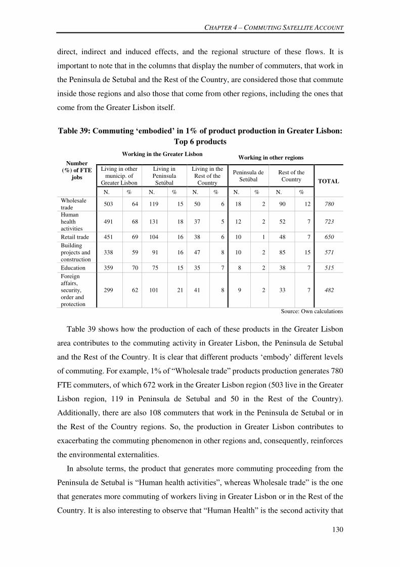
CHAPTER 4 – COMMUTING SATELLITE ACCOUNT
130
direct, indirect and induced effects, and the regional structure of these flows. It is
important to note that in the columns that display the number of commuters, that work in
the Peninsula de Setubal and the Rest of the Country, are considered those that commute
inside those regions and also those that come from other regions, including the ones that
come from the Greater Lisbon itself.
Table 39: Commuting ‘embodied’ in 1% of product production in Greater Lisbon:
Top 6 products
Number
(%) of FTE
jobs
Working in the Greater Lisbon
Working in other regions
Living in other municip. of
Greater Lisbon
Living in Peninsula Setúbal
Living in the Rest of the
Country
Peninsula de Setúbal
Rest of the Country TOTAL
N. % N. % N. % N. % N. %
Wholesale trade
503 64 119 15 50 6 18 2 90 12 780
Human health activities
491 68 131 18 37 5 12 2 52 7 723
Retail trade 451 69 104 16 38 6 10 1 48 7 650
Building projects and construction
338 59 91 16 47 8 10 2 85 15 571
Education 359 70 75 15 35 7 8 2 38 7 515
Foreign affairs, security, order and protection
299 62 101 21 41 8 9 2 33 7 482
Source: Own calculations
Table 39 shows how the production of each of these products in the Greater Lisbon
area contributes to the commuting activity in Greater Lisbon, the Peninsula de Setubal
and the Rest of the Country. It is clear that different products ‘embody’ different levels
of commuting. For example, 1% of “Wholesale trade” products production generates 780
FTE commuters, of which 672 work in the Greater Lisbon region (503 live in the Greater
Lisbon region, 119 in Peninsula de Setubal and 50 in the Rest of the Country).
Additionally, there are also 108 commuters that work in the Peninsula de Setubal or in
the Rest of the Country regions. So, the production in Greater Lisbon contributes to
exacerbating the commuting phenomenon in other regions and, consequently, reinforces
the environmental externalities.
In absolute terms, the product that generates more commuting proceeding from the
Peninsula de Setubal is “Human health activities”, whereas Wholesale trade” is the one
that generates more commuting of workers living in Greater Lisbon or in the Rest of the
Country. It is also interesting to observe that “Human Health” is the second activity that

CHAPTER 4 – COMMUTING SATELLITE ACCOUNT
131
generates more commuters working in the Peninsula de Setubal region and only the fifth
that embodies more commuters working in the Rest of the Country.
One unique characteristic strictly associated with the application of this methodology
allows for a new remarkable perspective of ‘commuting spillovers’. For example, 1% of
“Health Activities” production ‘embodies’ 131 commuters from the Peninsula de Setubal
to Greater Lisbon, but only 90 of these work directly in this industry, while the remaining
41 correspond to the ‘embodiment’ of commuters who live in the Peninsula de Setubal
and work in other industries located in the Greater Lisbon region. This outcome
specifically comes from incorporating the indirect and induced effects.
As the commuting intensity by industry, and by region, varies significantly, this
implies that each product’s production has the potential to affect commuting differently.
Thus, commuting resulting from indirect and induced effects should not be neglected.
There is a major reason for this conclusion: a significant share of the commuting flows
resulting from the production of a specific product can be linked to the industry and the
region that produces the inputs needed to satisfy the production.
To sum up, this research adds to the existing literature as it uncovers the commuting
effects associated with sectoral and interregional interdependencies, thereby opening up
new avenues for improving policy and decision-making processes in highly urbanized
regions and improving the impact assessment application to metropolitan regions.
4.11. Final Comments
The main goal of this PhD dissertation consists of transforming/adapting an MRIO
framework to assess the economic, social and environmental impacts of commuting. The
transformations include the introduction of regional distribution of income, the explicit
split of final household consumption into commuters and non-commuters, a specific
development of the real estate rental activity and the distribution of income that arises
from this economic activity, and, finally, the extension of the model to an energy and
environmental satellite account. All of the steps were described in this chapter.
The application of this advanced model in two ‘extreme’ scenarios allowed us to better
understand the consequences and impacts of commuting in a metropolitan setting. Indeed,
commuting by itself induces an important loss in economic activity. This outcome and
also the intensity of the effect may be different in other metropolitan areas located in
countries with a different economic structure, particularly when the commuting-related

CHAPTER 4 – COMMUTING SATELLITE ACCOUNT
132
products are mainly domestically produced. However, it is our belief that that this result
is remarkable to the Lisbon Metropolitan Area but also to the majority of metropolitan
areas in Western countries, particularly in Europe but also in other economies as Japan
and China. This mostly results from the different consumption structure between
commuters and non-commuters, since commuters have a consumption pattern that is
more intensive in products with a large share of international inputs embodied in their
production or inclusively that are almost exclusively imported. On the other hand,
commuting as part of a more embracing phenomenon has a relevant role in potentiating
the agglomeration economies in a given region, since it contributes to maintaining the
proximity of firms within a given CBD.
Additionally, the results in terms of real estate rents matter in macroeconomic terms.
However, this effect may be considered a small one, taking into account the size of
regional or national economies. Nevertheless, it can also imply an important distribution
of benefits/losses according to each type of economic agent located in the region/country.
In other words, landlords would be important beneficiaries of a situation where real estate
rents increase, following an agglomeration of the economic activity.
Moreover, the CSA modeling framework was also applied in a more ‘realistic’
scenario in which the ‘vacant’ houses located in the Lisbon municipality were occupied
by commuters. This also underlines a possible future use of this tool: applying it to
real-case studies in order to understand the additional cost/benefits of changes in
commuting patterns. The results of this empirical approach shed some light on the impacts
that result from promoting urban recentralization and the adoption of adequate tools and
urban planning strategies. Indeed, with this innovative modeling framework, commuters
and economic activity are integrated in the same framework and, as shown, the economic
multipliers can be converted into ‘commuter multipliers’.
Finally, the results obtained from the hypothetical scenarios and the hypothetical
reduction of ‘wasteful’ commuting point to important significant gains in terms of the
environment. Comparing all of the scenarios examined, the current situation is the one
where energy consumptions and CO2 emissions have the most important negative effects
at the environmental level.

133
“For many people, commuting is the worst part of the day, and policies that can make commuting shorter
(…) would be a straightforward way to reduce minor but widespread suffering.”
Daniel Kahneman, 2012
“Buy land, They don’t make it anymore”
Mark Twain
CHAPTER 5 – CONCLUSION
This PhD dissertation assumed the ambition of addressing one of the most globalized
urban phenomena, which determinately forges the lives of millions of human beings.
Commuting is more than simply travel, repeated every day, and usually taking a certain
amount of time and money, which, on a less fortunate day, can completely ruin someone’s
mood. An average commuter in the Lisbon Metropolitan Area spends approximately 10
months of their life travelling to work, by the time of his retirement. This is probably
more than the time consumed by other more ‘rewarding’ activities. Indeed, commuting is
one of the most important activities in the contemporary world, for three major reasons:
first, it is a vital ‘cost’ tolerated by households, as it allows them to earn their income;
second, it is crucial to the society as it provides the necessary workforce for the production
activity; and, finally, most of the time it is the byproduct of two of the most difficult
decisions made by households - the choice to buy/rent a house and the option to have a
certain job. So, commuting usually emerges as an undesirable consequence of these
meaningful dimensions.
Moreover, commuting has a key role in regional and urban economies. Commuting
affects the economy as much as (or even more than) other interregional economic flows
or possible external shocks. Commuting shapes the CBDs and defines their relationship
with neighboring regions. It changes households’ consumption patterns and exacerbates

CHAPTER 5 - CONCLUSIONS
134
fuel consumption and greenhouse gas emissions. As shown, the dialectical relationship
between commuting, territorial dimensions and economic activity raises the importance
of the marriage between urban modeling and more realistic frameworks that incorporate
(multi-dimensional) interdependencies. Society, academia and people demand advances
capable of shedding some light on these difficult but inspiring challenges. Accordingly,
in this dissertation several contributions were made.
5.1. Methodological and empirical contributions
Chapter 2 described several dimensions of the Lisbon Metropolitan Area (LMA). This
region comprises two NUTS III regions. Greater Lisbon is characterized by the location
of Lisbon, the Portuguese capital, while the other region – Peninsula de Setubal – is
typically referred to as a suburban region. Some demographic and economic indicators
were presented highlighting the unique characteristics of Greater Lisbon, as a region that
concentrates many productive industries (mainly services) and an important
concentration of several headquarters of national and multinational firms. Thus, the
analysis highlights an important trade balance surplus in the Greater Lisbon region
(mostly due to interregional trade). On the other hand, the trade balance of the Peninsula
de Setubal presents a large deficit that accounts for almost 30% of its GDP. This
significant deficit is (at least) in part balanced by the income resulting from commuting.
Indeed, an important share of commuters that live in the Peninsula de Setubal have their
salaries paid by the industries located in the Greater Lisbon region and “transfer” that
money to the Peninsula de Setubal region. Finally, the commuting activity in Portugal
and in the LMA was characterized. The LMA is the region where commuting is more
intensive, with 47% of the workers traveling to other municipalities in order to work. This
intensive commuting also occurs between municipalities located in the two margins of
the Tagus River. The large distances traveled by an important share of the commuters
contribute to the impressive amount of kilometers traveled by commuters every day in
the LMA (more than 35 million). As highlighted, different industries incorporate a
significantly distinct share of commuters among their workers. Indeed, while for some
industries around 70% of their workforce is composed of commuters (e.g. “Water
Transport”, “Air Transport”, “Computer Programming, Consultancy and related
activities”), for others the figure is less than 30% (e.g. “Agriculture”, “Fishing” and
“Manufacture of basic metals”). Furthermore, despite the relatively higher use of public

CHAPTER 5 - CONCLUSIONS
135
transportation in the LMA than in the ‘Rest of the Country’, it is very significant that most
of these workers commute by car.
Next, Chapter 3 was specifically devoted to the methodology used in the development
of the MRIO framework applied to the LMA. It started by presenting an overview of the
characteristics and procedures applied to compile the Input-Output (I-O) data at national
level. The official data provided by the National Statistical Institute provided the Use
Table at “purchasers’ prices” and “total flows”. So, the first step consisted of transforming
our national table to “basic prices” and “domestic flows”. According to the MULTI2C
practice, the procedures to ‘close’ the model to households living mainly on labor income
(employees and self-employed workers) were applied. So, the household consumption
was split into five different household types and the income paid by each industry as
compensation for employees and mixed-income was estimated. Next, from the national
table, 30 I-O regional tables were estimated, each one corresponding to a Portuguese
NUTS III region. These regionalization procedures made good use of detailed
information from several sources to estimate, on the one hand, the product supply at the
regional level and, on the other, the specific “use” of products (both as Intermediate
Consumption or Final Demand) in each of the regions. In the Intermediate Consumption
case, the consumption of industries was generally made applying the equal industry
technology assumption. Then, to derive the LMA MRIO model, the interregional trade
estimation was performed through the application of a pragmatic methodology, according
to products’ specific characteristics (tradable, non-tradable or others).
Chapter 4 was devoted to the conceptualization and then to the application of the
‘Commuting Satellite Account’ (CSA) framework. First, the process of estimating the
elements that integrated the CSA was explained, involving three particular features on
which that framework particularly focused: first, the interregional distribution of labor
income by region and household type, according to the journey-to-work data; second, the
distinct consumption structures of commuter and non-commuter households; and, finally,
the real estate rental activities considered in the endogenous part of the model (a share of
the income originated by this activity represents a transfer directly benefiting households,
particularly landlords but also, more marginally, those living mainly from labor income
and pensions). Next, all of these components were integrated together with an energy and
environmental extension, which allowed for assessing the impacts of certain shocks in
the (physical) quantity of primary energy used by each industry or household type, in
each region. These energy uses were then “converted” into corresponding CO2 emissions.

CHAPTER 5 - CONCLUSIONS
136
After that, the CSA framework was applied to estimate hypothetical scenarios,
considering changes in the commuting patterns of those that live and work in the Lisbon
Metropolitan Area. First, two ‘extreme’ scenarios were applied in order to assess the
opportunity costs of commuting. One scenario admitted the end of commuting, by
considering that workers change their place of residence to the municipality where they
work. The other scenario also admitted the hypothesis of commuting ceasing, but through
the increased dispersion of economic activities to the places where commuters live. These
scenarios demand a specific set of transformations in the input coefficients matrix and,
consequently, in the Leontief inverse. These modifications and algebraic procedures were
deeply explored in this chapter.
According to the results of the first scenario, if the current LMA commuters could live
closer to their workplace, important savings would emerge in terms of economic, social
and environmental (opportunity) costs. In this scenario, where agglomeration forces are
strengthened and density increases, the end of commuting flows and, consequently, a
change in households’ consumption structure, contributes to an expansion of the national
economy. So, for the LMA, the GVA loss in the suburbs (216 million Euros in the
Peninsula de Setubal and 43 million Euros in the ‘Rest of the Country’) is more than
offset by an increase in Greater Lisbon GVA (921 million Euros). The difference between
the benefits in Greater Lisbon and the losses in Peninsula de Setubal and the ‘Rest of the
Country’ indicate that the Portuguese GVA would increase by 0.5%. This is even more
relevant as energy consumption and CO2 emissions should simultaneously decrease
(about 0.7% of the national emissions). This is exclusively due to the reduction in the
consumption of “Oil and its derivatives”, as the economy expansion would lead to an
increase in the consumption of Natural Gas and Coal.
On the other hand, if commuting vanishes due to the economic activity dispersion
towards the suburbs, the economic consequences would be likely to be globally negative,
despite the increase in the suburbs’ economic production. So, the Peninsula de Setubal
and the ‘Rest of the Country’ GVAs would increase by more than 4,159 and 883 million
Euros, respectively. However, the decline in Greater Lisbon would be much more
significant leading to a 1.5% loss in national GVA. In terms of employment, the national
decrease would be less significant (approximately 0.5%) as the economy would be more
concentrated in less productive regions (and so, more workforce would be needed for the
same amount of Output). Thus, for the LMA case study, the results indicate that the
dispersion would imply a reduction in economic productivity that would overwhelm the

CHAPTER 5 - CONCLUSIONS
137
benefits of ending commuting. This scenario highlights an important trade-off between
economic and environmental effects, since it was estimated that national greenhouse gas
emissions would fall by almost 3%, thus indicating a substantial positive environmental
impact. Although an important share of this effect would result from the decline in the
economy, another part would result from a shift towards more ‘environmental friendly’
consumption.
As changes in urban density may affect real estate rental activities, the results of both
scenarios were tested through a sensitivity analysis. Accordingly, it was assumed that, in
the scenario where households change their place of residence, housing rents in the
Greater Lisbon region would increase. Alternatively, in the scenario where firms
reallocate to the suburbs, the rents supported by industries in the Peninsula de Setubal
would rise. Despite the substantial changes in the real estate rental effort, the results
broadly confirm the findings highlighted above and produce a relatively small change in
macroeconomic indicators. The main reason is that while rents are considered a cost
supported by households or firms, they are also an income that favors some economic
agents that provide this specific service. Thus, in macroeconomic terms, this specific
expenditure does not represent such a significant burden on the economy. Nevertheless,
the macro analysis conceals the fact that changes in real estate rental activity may
unbalance the income distributed among households or firms. Indeed, if higher real estate
rental prices are an outcome of the agglomeration process then it is predictable that
landlords and financial institutions (who are also major producers of the rental services)
are the ones that would obtain the major benefit from this side-effect. Finally, the
comprehensive analysis of both scenarios indicates dichotomous, yet complementary,
conclusions: commuting, by itself, induces significant economic, social and
environmental costs, and commuting as one of the many elements arising from the
agglomeration phenomenon is undoubtedly linked to processes of increasing productivity
and economic expansion. Additionally, commuting imposes important environmental
costs. These important conclusions have major relevance and should materialize in a more
adequate set of policies and recommendations that can accurately contribute to
accomplishing the 11st Sustainable Development Goal of the UN 2030 Agenda (UN,
2015).
In a second application, the CSA framework was applied to assess a ‘more realistic’
scenario. It was considered that a share of the ‘unoccupied’ houses in the Lisbon
municipality would be inhabited by commuters (who, therefore, would become non-

CHAPTER 5 - CONCLUSIONS
138
commuters). So, the simple reallocation of 4% of the LMA commuters (about 25
thousands persons) would generate a total gain of 0.04% of national GVA. This
redistribution of people would be (basically) from the other regions to Greater Lisbon,
which would result in its economic expansion, while this declined in the others.
Additionally, the major share of the reallocation would be within the Greater Lisbon
region, which justifies why its benefits would exceed in a widespread manner the other
regions’ losses. In a similar mode to the first ‘extreme’ scenario of a commuting
opportunity costs appraisal, two main reasons explain the national expansion in GVA.
First, when commuters become non-commuters this implies changes in the consumption
demand composition, from products with larger imports content (vehicles, fuel, etc.) to
others comprising a larger share of nationally generated value added. The second reason
is that when ex-commuters change their place of residence to the Greater Lisbon region,
they are deemed to behave as Lisbon residents. This means that, for example, they
demand more services, which have a higher average GVA/Output ratio, while adopting
the ‘propensity to consume’ of their new region. Once more, the results of this more
‘realistic’ scenario reinforce the conclusion that commuting has important costs that must
be addressed by decision-makers at the local and regional levels.
Finally, the CSA is a suitable tool to assess the impacts of multiple changes in the
exogenous final demand. In the latest application presented in Chapter 4, an increase of
1% in the demand directed towards product production in the Greater Lisbon region was
considered. In this application, the proposed CSA multipliers matrix was different from
the one that would result from a more ‘traditionalistic’ approach, as it included a broader
set of income flows. Ultimately, this also resulted in distinct income and employment
multipliers matrices. Actually, one important step forward presented in section 4.10
comprised the estimation of a so-called ‘commuter multipliers matrix’ and the estimation
of the ‘commuting embodied’ in the production in Greater Lisbon.
This work sets out an innovative approach to study the complexity of commuting flows
and their impacts. The proposed CSA framework is expected to be a decisive step in this
direction. For this, the CSA has been specifically designed to assess changes in workers’
commuting patterns that affect the regional distribution of labor income, household
consumption patterns and real estate rental activities. The integration of a CSA into the
mainstream multi-regional input-output framework allows for the study of a wide range
of interactions anchored in the specific reality of a given geographical territory. Thus,

CHAPTER 5 - CONCLUSIONS
139
while deviating from more ‘theoretical’ approaches it makes an important contribution
through the application of a more ‘down-to-earth’ framework in the field of urban studies.
Moreover, the CSA takes a step forward with regard to traditional sectoral
interdependencies by modeling the income sprawl throughout the territory, taking into
account commuting flows and rental activities. The CSA application to the Lisbon
Metropolitan Area illustrates the contribution of commuting patterns to shaping urban,
regional and even national economies.
The framework developed opens up new research avenues to assess structural changes
in urban tissues, commuting patterns and housing or workplace locations. Indeed, the
outcome of this PhD dissertation sheds light on some possible policy designs that would
encourage economic growth, and simultaneously increase well-being and a more
sustainable urban environment. This work integrates (and reinforces) a set of works that
have stated the importance of implementing coherent and effective urban planning that
on the one hand, acknowledges the opportunity costs of commuting (and, consequently,
of urban sprawling), and, on the other hand, does not ignore the benefits of economic
agglomeration. Ceasing commuting is an unreachable and, even, undesirable
accomplishment, but to manage commuting and reduce sprawling looks possible and is
dependent on of our capability to implement the proper changes. Of course, in historical
CBDs, such as the one located in the Lisbon municipality, the increasing agglomeration
must also look to protect historic buildings and cultural heritage. This ‘will’ to change
our cities will definitely require a considerable break with past and current practices,
imposing the application of specific measures, as advanced below.
5.2. Policy Recommendations
Next, some policy recommendations are addressed and some critical findings are
analyzed, to reach conclusions at a more general level and others focusing more
specifically on the Portuguese reality.
1. Urban and regional planning matters. Despite the fact that the decision to buy a
house with certain characteristics, in a specific location, should belong to the
personal sphere of every household, the urbanization process produces ‘winners
and losers’. Moreover, the trillions of variables weighted billions of times to
support the decision of millions of households living in a given city (may) actually

CHAPTER 5 - CONCLUSIONS
140
not lead to the best societal outcome. As commuting will continue to exist in
modern societies, it cannot continue to be ‘swept under the carpet’ and more active
policies should be applied to reduce it, in order to minimize its negative
consequences. So, it is our belief that active planning (correctly performed and
applied) may improve life in urban spaces. Ewing (1997: 118) considers that “the
posture usually assumed by local governments (…), waiting for property owners
to come forward with rezoning requests is not planning but reacting”. Moreover,
Hamilton and Röell (1982) had already stated several ‘market failures’ that
generate ‘wasteful’ commuting and that justify public regulation. So, the role of
planning arises as a mechanism to intervene in the market processes to achieve
broader aims that should be clearly stated and widely acknowledged.
2. Planning should be made at the correct level of governance. According to Brenner
(1999) the political-regulatory institutions of urban regions are often fragmented
into multiple agencies and departments with distinct jurisdictions and tasks. So,
contemporary discussions on regional governance must emphasize the need for
administrative flexibility and regionally coordinated economic development
strategies as a way to minimize some cases of interspatial competition. In Portugal,
urban policies have been mostly outlined at the municipal level. This is even more
problematic, as it often results in different actors defining policies that in the end
lead to contradictory results. The most striking point is that some suburban
municipalities actively compete to attract inhabitants and determinately contribute
to enhancing the cost of commuting. For example, Almeida et al. (2013) reported
the case of a Portuguese municipality where policy makers considered that higher
tax rates (despite their value is well below the effective cost supported by public
authorities) may constitute a relevant loss in regional competitiveness and reduce
its attractiveness. Accordingly, many local policy makers admit to often comparing
their tax rates with the ones practiced in their neighboring regions. In fact, the
policy makers ‘rational’ option is very often to promote extensive land-use, settling
new suburban neighborhoods, and in this way increasing their budgets and political
influence. This may be even truer in the suburbs, where land is abundant and
relatively cheap and many of the investments and infrastructures required to
sustain this new construction (e.g. water, road, public facilities) are financed by the
central government. This highlights the fact that the attribution of wider

CHAPTER 5 - CONCLUSIONS
141
responsibilities, concerning urban and regional planning, to inter-municipal and/or
regional authorities, will definitely contribute to reducing the competition between
municipalities and increase the potential benefits of a coherent urban policy.
3. Land-use Policy can favor less sprawled regions and, consequently, less
commuting. One must be aware that the national legal background in Portugal is
different from that prevailing in most European countries. According to Newman
and Thornley (1996), for historical reasons the Portuguese case represents one of
the most underdeveloped urban planning systems. Carvalho and Oliveira (2015)
also consider that the Portuguese municipalities benefit from a large (and
discretionary) margin to state that a certain area of land as urban or available for
future construction. Moreover, due to the “fragmented and sprawled infrastructural
occupation in Portugal, during the last decades, the zones classified as urban (or
where building is admissible) correspond to very extensive areas” (Carvalho and
Oliveira, 2015: 3)69. This had already been acknowledged in the National Program
for Territorial Planning and Management (PNPOT, 2007), as it refers to the need
to reduce the urban areas in Portugal. The extension of land that has been classified
as “urban” or “passible for being constructed” is so much sprawled that Mateus
(2007) considered that the urban perimeters in Portugal could accommodate more
than 30 million inhabitants (three times more the Portuguese population). So,
building construction and, consequently, the urbanization process become
exclusively dependent on private initiatives, implying in many cases that the
‘rational and individual’ decision of the investor leads to the use of the
‘unoccupied’ lands located in the suburbs (since they are less expensive). From
this political and institutional framework an additional problem arises. As most of
the land is privately owned and the initiative to build belongs to property owners,
the ‘rational’ decision of the landowner of more central places can be simply to
maintain the land as vacant and sell it in the future, independently of the costs
supported by the society (inclusively the commuting costs). Although this question
seems to have been largely ignored (at least in Portugal), two important pieces of
work addressed this issue decades ago. Bahl (1968) considers that if a city is
69 A new Law (31/2014) and a Decree-Law (80/2015) have recently been approved and new restriction to
the (re)classification of soil was imposed on municipalities. However, it does not directly imply the significant reduction of the zones already classified as urban.

CHAPTER 5 - CONCLUSIONS
142
expected to grow and there are expectations that the land value will continue to
increase, then the landowner will continue to keep (and eventually add) his stock
of land until an increasing expected future return from an alternative investment
emerges. On the other hand, Clawson (1962: 108) has a more straightforward view
of the landownership problem in central cities and considers that “land speculation,
sprawl and intermingled idle land are all natural outgrowths of economic and
institutional forces (…). Policies should be applied to minimize the impact of land
speculation”. In practical terms, the differences between the Portuguese
institutional framework and other European frameworks can be easily observed.
Taking the Netherlands as an example Van der Krabben and Jacobs (2013)
describe the land development strategy. The process begins by involving public
purchase, ownership and active planning for land use before a certain parcel is
released for actual development to the private sector. They argue that this
guarantees building developments according to public policies, while ensuring full
cost recovery for all public works (through the sale of building plots).
Simultaneously, at least part of the surplus value of the land is captured by the
public sphere. Otherwise in Portugal, urban growth has been left to private
initiatives. Land is private from the beginning until the end of the process. The
application of more restrictive regulatory legislation could have reduced the
construction of new building lots in the suburbs and redirected some of the
investment made in new construction to the refurbishment of old city areas and a
downtown renaissance. So, commuting expansion could be (to a certain point)
avoided.
4. Transport Policy is a central issue in urban governance. The decision to become a
commuter is to a large extent dependent on transportation costs. When local,
regional or federal governments decide to build a new highway or a bridge or to
finance public transportation, in fact they are using taxes to favor those that will
use such infrastructures more intensively. On the contrary, when the burden falls
on the commuter (at least in the long term) commuting is discouraged. So, in a
more sprawled city, where car commuting prevails, one may have a case to
implement measures that can condition car use. Indeed, the recent decrease in oil
prices, which could lead to important and sustained deflation in fuel prices, has
reduced the costs supported by those that commute by car and contributed to

CHAPTER 5 - CONCLUSIONS
143
increasing commuting attractiveness. Accordingly, the argument runs that national
governments should mitigate this recent decrease in fuel prices and maintain the
prices at a significant level. This can be done through fiscal policy on “oil and its
derivatives” or through the introduction of taxes or fees that are in turn applied to
improve the quality of life of those living in the CBD. These measures can be
complemented by, for example, the introduction of congestion tolls (already
applied, with different specifications, in London, Singapore, Durham or Milan).
As introducing congestion tolls is often politically difficult, alternatively, parking
policies could be applied to reduce traffic in the city center (Verhoef et al. 1995;
Barata et al., 2011). In this case, the recommendation would be to give priority to
non-commuters living in the CBD, in occupying the limited number of parking
places available there. Initiatives such as park and ride (Mingardo, 2013), car-
sharing and car-pooling (Correia and Antunes, 2012) can also be encouraged
among those that live or travel to the CBD. A collateral or even the main purpose
of this type of policy usually consists of triggering a change in the means of
transportation used in commuting and it is not so much directed to reduce
commuting as argued in this thesis (although a non-explored topic is that different
commuting modes imply different costs). Without doubt, while roads and
highways are built to reduce congestion, it seems that these infrastructures also
contribute to exacerbating commuting. Indeed, Carvalho et al. (2013) consider that
the process of building new roads should be globally suspended or else sprawling
will continue to increase.
5.3. Limits and Future Research
Throughout this study it has become clear that the lack of statistical data requires
making several (yet, as we believe, feasible) assumptions. Some examples concern the
regionalization of the I-O tables and the estimation of interregional trade between Greater
Lisbon, the Peninsula de Setubal and the ‘Rest of the Country’. Moreover, it would
certainly be preferable to have used more detailed information concerning the commuter
and non-commuter households’ consumption structures and data regarding the regional
distribution of real estate rental income flows. Of course, these information gaps have
limited the analysis, restricting not only the quantity, but also the quality, of the
information provided for policy purposes. Unquestionably, Portuguese National and

CHAPTER 5 - CONCLUSIONS
144
(mostly) Regional Accounts need to continue to improve with regard to the quality of
data, in order to allow for more accurate specification of the intricate complex interactions
between geography and the economy in Portugal. The same applies to the data
(un)availability concerning regional primary energy consumption and CO2 emissions.
Nevertheless, future work can be performed using the ‘Commuting Satellite Account’
framework either based on the LMA tri-regional model or by adapting the procedure to
other metropolitan regions, as many research topics still remain unexplored. On the one
hand, this could imply some refinements and methodological advances applied in the
context of the CSA framework, such as:
Extension of the model to incorporate other satellite information of major
importance to assist policy-makers on an urban scale, namely e.g. water, waste
disposal, land-use.
Extension of the model to embrace a higher number of regions. Moreover, it is
the author’s belief that the estimation of international and interregional trade
and the comprehensive analysis of the corresponding results would largely
benefit from detaching the Lisbon municipality from the Greater Lisbon region
and from its consideration as an independent region.
A higher level of households demand disaggregation. Namely, commuters’
consumption patterns could be split according to the means of transportation
used or according to other social or demographic characteristics (e.g. age,
number of members in the household, housing type).
To perform the analysis for more recent years and assess the structural changes
(through some form of structural decomposition analysis and/or disaggregation
techniques), which might have occurred in the Greater Lisbon region.
To incorporate this model into an even more comprehensive framework,
making use of the sophisticated techniques associated with Geographical
Information Systems, allowing for the integration of transport networks, traffic
simulation and mixed land-uses.
To consider the existence of non-linear relations between land availability,
commuting and housing prices. This will certainly demand much more data
availability and/or the assumption of additional hypotheses concerning the
relations and elasticities affecting these dimensions, but it would certainly

CHAPTER 5 - CONCLUSIONS
145
improve the richness of the analysis addressed. This would also be a step
forward for a discussion of the optimum level of commuting.
On the other hand, the CSA modeling framework could also be applied to perform
other empirical assessments of national and/or regional impacts resulting from, for
example:
A disruption in commuter flows in the Lisbon municipality due for example,
to a disaster on one of the two bridges crossing the River Tagus at Lisbon or a
persistent strike in the boat transportation services).
The introduction of traffic and transport demand management constraints
and/or technological changes in private transportation and/or an increase in the
public transport network, which would induce changes in the modal split.
The computation of high-order economic costs or benefits that might result
from an expansion in the road, train or underground network.
5.4. Final Words
To conclude, decisive changes from the status quo are required to contain sprawling
in most of the large metropolitan areas worldwide, as in the Lisbon case. The author of
this dissertation definitely believes that the existing reality has harmed the economy, the
environment and the lives of millions of workers, who, every day, spend an important
share of their time inside their car or on public transportation. As cities are increasingly
the ‘home’ of more and more humans, it is time to move towards a new institutional and
legal framework to allow for living in a human settlement that:
Provides shelter for all its inhabitants;
Provides jobs and employment at an acceptable distance;
Allows for substituting the time spent commuting with more interesting and
rewarding activities;
Provides access to affordable, accessible and sustainable transport systems;
Reduces the environmental impact of its activities and addresses air quality
issues;
Provides universal access to safe, inclusive and accessible green and public
spaces.

CHAPTER 5 - CONCLUSIONS
146
Supports positive economic, social and environmental links between urban,
peri-urban and rural areas through the implementation of regional and urban
development planning.
Such prosperous, culturally intense, healthier and sustainable cities would not be easy
to raise. However, mankind is continuing to evolve and it has been capable of many
astonishing achievements. In a period where the economic challenges seem to
circumscribe to uninspired goals such as austerity and a reduction in public spending,
society needs to step forward and assume that a better future must galvanize more efforts,
more involvement and audacity.
147
REFERENCES
Ahlfeldt, G. (2011) The train has left the station: do markets value intracity access to
intercity rail connections? German Economic Review, 12(3), 312-335.
Alonso, W. (1964) Location and land use: toward a general theory of land rent. Harvard
University Press, Cambridge, USA.
Almeida, E., E. Haddad and G. Hewings (2010) Transport–regional Equity Issue
Revisited. Regional studies, 44(10), 1387-1400.
Almeida, J., B. Condessa, P. Pinto, P and J. Ferreira (2013) Municipal Urbanization Tax
and Land-use Management - The case of Tomar, Portugal. Land Use Policy, 31,
336-346.
Anas, A. and I. Kim (1996) General Equilibrium Models of Polycentric Urban Land Use
with Endogenous Congestion and Job Agglomeration. Journal of Urban
Economics, 40(2), 232-256.
Anas, A. and Y. Liu (2007) A Regional Economy, Land Use and Transportation Model
(RELU-TRAN): Formulation, Algorithm Design and Testing. Journal of Regional
Science, 47(3), 415-455.
Anas, A. (2013) A Summary of the Applications to date of RELU-TRAN, a
Microeconomic Urban Computable General Equilibrium Model. Environment
and Planning B: Planning and Design, 40(6), 959-970.
Angel, S. and A. Blei (2016) The Spatial Structure of American Cities: The Great
Majority of Workplaces are no longer in CBDs, Employment Sub-centers, or
Live-work Communities. Cities, In Press.
Arnott, R. and J. MacKinnon (1978) Market and Shadow Land Rents with
Congestion. The American Economic Review, 68(4), 588-600.
Aroca, P. (2001) Impacts and Development in Local Economies based on Mining: the
case of the Chilean II region. Resource Policy, 27(2), 119–134.
Aroca, P. and M. Atienza (2011) Economic Implications of Long Distance Commuting
in the Chilean Mining Industry. Resources Policy, 36, 196-203.
Bahl, R. (1968) A Land Speculation Model: The Role of the Property Tax as a Constraint
to Urban Sprawl. Journal of Regional Science, 8(2), 199-208.
Bajari, P. and M. Kahn (2005) Estimating Housing Demand with an Application to
Explaining Racial Segregation in Cities. Journal of business and economic
statistics, 23(1), 20-33.

REFERENCES
148
Barata, E., L. Cruz and J.-P. Ferreira (2011a) Parking at the UC campus: Problems and
solutions. Cities, 28(5), 406-413.
Barata, E., L. Cruz, A. Sargento, P. Ramos and J.-P. Ferreira (2011b) Deriving Regional
Input-Output Matrices to Assess Impacts in Small Portuguese Peripheral Regions.
In: Sectores estrategicos para un nuevo modelo economico, IV Jornadas
Españolas de Análisis Input-Output, Cámara, A., Cardenete, M., Medina, A.,
Monrobel, J. (eds.). Universidad Rey Juan Carlos, Madrid, Spain.
Barrett, G. (1996) The Transport Dimension. In: The Compact City: A Sustainable Urban
Form?, M. Jenks, E. Burton, K. Williams (eds.), 171–180, E&FN Spon
Publishers, London and New York,
Batterman, S., A. Martins, C. Antunes, F. Freire and M. da Silva (2011) Development
and Application of Competencies for Graduate Programs in Energy and
Sustainability. Journal of Professional Issues in Engineering Education and
Practice, 137(4), 198-207.
Bayer, P., H. Fang and R. McMillan (2014) Separate when equal? Racial Inequality and
Residential Segregation. Journal of Urban Economics, 82, 32-48.
Beckmann, M. (1973) Equilibrium Models of Residential Land use. Regional and Urban
Economics, 3, 361-8.
Bhattacharjee A., E. Castro and J. Marques (2012) Spatial Interactions in Hedonic Pricing
Models: The Urban Housing Market of Aveiro, Portugal. Spatial Economic
Analysis, 7(1), 133-167.
Blackwell, J. (1978) Disaggregation of the Household Sector in Regional Input-Output
Analysis: Some Models Specifying Previous Residence of Worker. Regional
Studies, 12, 367–377.
Blundell, R. and T. Stoker (2005) Heterogeneity and Aggregation. Journal of Economic
Literature, 43(2), 347-391.
Bocarejo J.-P., I. Portilla and M. Pérez (2013) Impact of Transmilenio on Density, Land
Use and Land Value in Bogotá. Research in Transportation Economics, 40(1),
78-86.
Boussauw, K. and F. Witlox (2009) Introducing a commute-energy performance index
for Flanders. Transportation Research Part A: Policy and Practice, 43(5),
580-591.
Boustan, L. (2013) Racial Residential Segregation in American Cities. National Bureau
of Economic Research, Working Paper Nº 19045.
Brenner, N. (1999). Globalization as Reterritorialization: the Re-scaling of Urban
Governance in the European Union. Urban studies, 36(3), 431-451.

REFERENCES
149
Brown, L. and E. Moore (1970) The Intra-urban Migration Process: a Perspective.
Geografiska Annaler, series B, Human Geography, 52(1), 1–13.
Brueckner, J. and H. Kim (2003) Urban sprawl and the property tax. International Tax
and Public Finance, 10(1), 5-23.
Camagni, R., M. Gibelli and P. Rigamonti (2002) Urban mobility and urban form: the
social and environmental costs of different patterns of urban
expansion. Ecological Economics, 40(2), 199-216.
Cameron, G. and J. Muellbauer (1998) The Housing Market and Regional Commuting
and Migration Choices. Scottish Journal of Political Economy, 45, 420-446.
Carvalho, J. (2013) Ocupação Dispersa: Custos e Benefícios à Escala Local. Direcção
Geral do Território, Lisboa, Portugal.
Carvalho, J. and F. Oliveira (2015) Classificação e Requalificação do Sólo Urbano no
Novo Quadro Legal. Associação de Estudos de Direito Regional e Local. Braga,
Portugal.
Cervero, R. (1989) Jobs-housing balancing and regional mobility. Journal of the
American Planning Association, 55(2), 136-150.
Cervero, R. and K. Wu (1997) Polycentrism, commuting, and residential location in the
San Francisco Bay area. Environment and Planning A, 29(5), 865-886.
Chin, H. and K. Foong (2006) Influence of School Accessibility on Housing
Values. Journal of Urban Planning and Development, 132(3), 120-129.
Cho, S.-H., J. Bowker and W. Park (2006) Measuring the Contribution of Water and
Green Space Amenities to Housing Values: an Application and Comparison of
Spatially Weighted Hedonic Models. Journal of Agricultural and Resource
Economics, 31(3), 485-507.
Choi, T. (2015) Understanding Environmental Responsibility of Cities and Emissions
Embodied in Trade. Economic Systems Research, 27, 133-153.
Clawson, M. (1962) Urban Sprawl and Speculation in Suburban Land. Land
Economics, 38(2), 99-111.
Correia, G. and A. Antunes (2012) Optimization Approach to Depot Location and Trip
Selection in One-way Carsharing Systems. Transportation Research Part E:
Logistics and Transportation Review, 48(1), 233-247.
Cruz, L., J. Proops, and P. Safanov (2005) Input-Output Models. In: Modelling in
Ecological Economics, J. Proops and P. Safanov (eds.), 36-57.Cheltenham:
Edward Elgar Publishing.

REFERENCES
150
Cruz, L. (2009) Application of IO Energy Analysis for CO2 Emissions by the Portuguese
Economy. In: Handbook of Input-Output Economics in Industrial Ecology-Eco-
Efficiency in Industry and Science, S. Suh (ed.), 23, 507-532. Springer.
Cruz, L. and E. Barata (2012) Hybrid IO Analysis of CO2 Emissions: An Application to
the Portuguese Economy. In: Air Pollution: Economic Modelling and Control
Policies. M. Llop (ed.), 65-95. Environmental Sciences Series. Bentham Science
Publishers.
Cruz, L., A. Parreiral, P. Ramos and E. Barata (2015) Economic and Environmental
Assessment of Energy Efficiency scenarios: A MULTI2C application.
Conference Proceedings of the 6th Spanish Conference on Input-Output Analysis.
Barcelona, Spain.
Day, J. and R. Cervero (2010) Effects of Residential Relocation on Household and
Commuting Expenditures in Shanghai, China. International Journal of Urban and
Regional Research, 34(4), 762-788.
De Bruyne, K. and J. Van Hove (2013) Explaining the Spatial Variation in Housing
Prices: an Economic Geography Approach. Applied Economics 45(13), 1673-
1689.
De Mesnard, L. (2004) Understanding the Shortcomings of Commodity‐based
Technology in Input–Output Models: an Economic‐Circuit Approach. Journal of
Regional Science, 44(1), 125-141.
Delgado, A. and I. Godinho (2011) Medidas de Localização das Actividades e de
Especialização Regional. In: Compêndio de Economia Regional, J. Costa, T.
Dentinho and P. Nijkamp (eds.), 15-35. Cascais, Portugal.
Dias, A. (2008) Sistema Integrado de Matrizes Input-Output para Portugal. Departamento
de Prospectiva e Planeamento e Relações Internacionais. Lisboa, Portugal.
Druckman, A. and T. Jackson (2009) The Carbon Footprint of UK Households
1990-2004: a Socio-economically Disaggregated, Quasi-multi-regional
Input-output Model. Ecological Economics, 68(7), 2066-2077.
EDP Produção (2011) Environmental Statement 2010 – Sines Thermoelectric Power
Plant (Portuguese only), Directorate of Thermal Production - EDP Gestão da
Produção de Energia, S. A., Sines, Portugal.
EDP Produção (2012) Environmental Statement 2011 – Ribatejo Thermoelectric Power
Plant (Portuguese only), Directorate of Thermal Production - EDP Gestão da
Produção de Energia, S. A., Carregado, Portugal.
EDP Produção (2013) Environmental Statement 2012 – Lares Thermoelectric Power
Plant (Portuguese only), Directorate of Thermal Production - EDP Gestão da
Produção de Energia, S. A., Figueira da Foz, Portugal.

REFERENCES
151
EEM (2008) Vitória Thermoelectric Power Plant (Portuguese only), Empresa de
Eletricidade da Madeira, S.A. – Directorate of Production Services, Funchal,
Portugal.
EEM (2011) Annual Report 2010, Empresa de Eletricidade da Madeira, Funchal,
Portugal.
Ejdemo, T. and P. Söderholm (2009) The Regional Economic Impacts of Mining: The
Case of Northern Sweden. 8th International Conference on Acid Rock Drainage
and Securing the Future: Mining, Metals and the Environment in a Sustainable
Society. 22-26 June, Skelleftea, Sweden.
Eom, T., W. Duncombe, P. Nguyen-Hoang and J. Yinger (2014) The Unintended
Consequences of Property Tax Relief: New York’s STAR Program. Education Finance and Policy, 9(4), 446-480.
EUROSTAT (2013) European System of National and Regional Accounts – ESA 2010.
Publications Office of the European Union, Luxembourg.
Ewing, R. (1997) Is Los Angeles-style Sprawl Desirable? Journal of the American
Planning Association, 63, 107-126.
Ewing, R., R. Pendall and D. Chen (2003) Measuring sprawl and its transportation
impacts. Transportation Research Record: Journal of the Transportation Research
Board, 1831, 175-183.
Ferreira, J.-P., R. Pina and P. Ramos (2012) Distâncias e Acessibilidades na Região
Centro. Boletim Trimestral da CCDRC. Coimbra, Portugal.
Ferreira, J.-P., E. Barata, P. Ramos and L. Cruz (2014a) Economic, Social, Energy and
Environmental Assessment of Inter-municipality Commuting: The case of
Portugal. Energy Policy, 66, 411-418.
Ferreira J.-P., P. Ramos, L. Cruz and E. Barata (2014b) Spill-over Effects in the
Portuguese Economy: Lisbon Metropolitan Area vs. Rest of the Country. 22th
International Input-Output Association Conference Proceedings, Lisbon,
Portugal.
Ferreira, J.-P., P. Ramos, L. Cruz and E. Barata (2015a) The Impacts of an ‘Urban Recentralization’ Scenario - a Commuting Satellite Account in a MRIO
Framework. 6th Spanish Conference on Input-Output Analysis, Barcelona, Spain.
Fertagus (2012) Relatório e Contas – 2010 (Portuguese only). Lisboa, Portugal.
Flegg, A. and C. Webber (1997) On the Appropriate Use of Location Quotients in
Generating Regional Input‐Output Tables: Reply. Regional studies, 31(8),
795-805.
REFERENCES
152
Flegg, A. and C. Webber (2000) Regional Size, Regional Specialization and the FLQ
Formula. Regional Studies, 34(6), 563-569.
Floater, G., P. Rode, A. Robert, C. Kennedy, D. Hoornweg, R. Slavcheva and N. Godfrey,
(2014) Cities and the New Climate Economy: the transformative role of global
urban growth. New Climate Economy Cities, Paper 01. LSE Cities, London
School of Economics and Political Science, London, UK.
Frade, I., A. Ribeiro, G. Gonçalves and A. Antunes (2011) An Optimization Model for
Locating Electric Vehicle Charging Stations in Central Urban Areas.
Transportation Research Record: Journal of the Transportation Research
Board, 3582, 1-19.
Fujita, M. (1989) Urban Economic Theory: Land use and City Size. Cambridge
University Press, New York, USA.
Fujita, M., P. Krugman, and T. Mori (1999) On the Evolution of Hierarchical Urban
Systems. European Economic Review, 43(2), 209-251.
Gardner, T. and M. Marlay (2013) Whither the Jobs : Identifying Concentrations of Employment in Metropolitan Areas. Urban Geography, 34, 37-41.
Gately, I. (2014) Rush Hour: How 500 Million Commuters Survive the Daily Journey to
Work. Head of Zeus, London, UK.
GEP-MTSS (2011) Quadros de Pessoal (Portuguese only), Database of the Office for
Strategy and Planning – Ministry of Labour and Social Solidarity.
Glaeser, E. and M. Kahn (2003) Sprawl and Urban Growth - Handbook of Urban and
Regional Economics, 4, 2481–2527.
Golob, T. and D. Hensher (1998) Greenhouse Gas Emissions and Australian Commuters'
Attitudes and Behaviour Concerning Abatement Policies and Personal
Involvement. Transportation Research, Part D: Transport and the Environment, 3,
1-18.
Gordon, P. and H. Richardson (1997) Are compact cities a desirable planning goal?
Journal of the American Planning Association, 63(1), 95-106.
Haddad, E. and E. Teixeira (2015). Economic impacts of natural disasters in megacities:
The case of floods in São Paulo, Brazil. Habitat International, 45, 106-113.
Haddad E., G. Hewings, A. Porsse, E. Van Leeuwen and R. Vieira (2015) The
Underground Economy: Tracking the Higher-order Economic Impacts of the São
Paulo Subway System. Transportation Research Part A: Policy and Practice, 73,
18-30.
Hamilton, B. and A. Röell (1982) Wasteful Commuting. The Journal of Political
Economy, 90(5), 1035-1053.

REFERENCES
153
Hanushek, E. and J. Quigley (1978) An Explicit Model of Intra-metropolitan
Mobility. Land Economics, 54(4), 411-429.
Harrigan, F., J. McGilvray and I. McNicoll (1981) The Estimation of Interregional Trade
Flows. Journal of Regional Science, 21(1), 65-78.
Haurin, D. and D. Brasington (1996) School quality and real house prices: Inter-and
intrametropolitan effects. Journal of Housing Economics 5(4),351-368.
Hewings, G. and R. Jensen (1986) Regional, Interregional and Multiregional Input-output
Analysis. Handbook of Regional and Urban Economics, 1, 295-355.
Hewings, G., Y. Okuyama and M. Sonis (2001) Economic Interdependence Within the
Chicago Metropolitan Area: A Miyazawa Analysis. Journal of Regional Science,
41, 195-217.
Hewings, G. and J. Parr (2007) Spatial Interdependence in a Metropolitan Setting. Spatial
Economic Analysis, 2(1), 7-22.
Hilgemberg, E. and J. Guilhoto (2006) Uso de Combustíveis e Emissões de CO2 no Brasil:
um Modelo Inter-regional de insumo-produto. Nova Economia, 16(1), 49-99.
ICFN (2013) Portuguese National Forest Inventory. Nature Conservation and Forests
Edition, Lisbon, Portugal.
INE (2003) Portuguese Census 2001. Database of the Official Statistics Portal, Statistics
Portugal, Lisbon, Portugal.
INE (2011a) Portuguese National Accounts 2007 (Base 2006). Statistics Portugal –
National Accounts, Lisbon, Portugal.
INE (2011b) Transport Statistics 2010. Statistics Portugal, Lisbon, Portugal.
INE (2011c) Statistical Yearbook of the Lisbon Region 2010. Statistics Portugal, Lisbon,
Portugal.
INE (2011d) Agricultural Census 2009 - Final results. Statistics Portugal, Lisbon,
Portugal.
INE (2012a) Portuguese National Accounts 2010 (Base 2006). Statistics Portugal –
National Accounts, Lisbon, Portugal.
INE (2012b) Portuguese Regional Accounts 2010. Statistics Portugal – National
Accounts, Lisbon, Portugal.
INE (2012c) Portuguese Census 2011. Database of the Official Statistics Portal, Statistics
Portugal, Lisbon, Portugal.
INE (2012b) Household Budget Survey - 2010/2011. Statistics Portugal, Lisbon,
Portugal.

REFERENCES
154
INE (2013a) Study on the Local Purchasing Power 2011. Statistics Portugal, Lisbon,
Portugal.
INE (2013b) Entrances by Road border of non-residents same-day visitors by place of
residence and purpose of journey. Database of the Official Statistics Portal,
Statistics Portugal, Lisbon, Portugal.
INE (2015a) Gross production of electricity (kWh) by Geographic localization (NUTS -
2002) and Type of electricity production. Database of the Official Statistics Portal,
Statistics Portugal, Lisbon, Portugal.
INE (2015b) Electricity production (kWh) in cogeneration plants by Geographic
localization (NUTS - 2002). Database of the Official Statistics Portal, Statistics
Portugal, Lisbon, Portugal.
IPCC (2006) 2006 IPCC Guidelines for National Greenhouse Gas Inventories. Prepared
by the National Greenhouse Inventory Program, H. Eggleston, L. Buendia, K.
Miwa, T. Ngara T. and K. Tanabe K. (eds). IGES, Japan.
Jun, M. (1999) An Integrated Metropolitan Model Incorporating Demographic-
Economic, Land-use and Transport Models. Urban Studies, 36, 1399-1408.
Jun, M. (2004) A Metropolitan Input-Output Model: Multisectoral and Multispatial
Relations of Production, Income Formation, and Consumption. The Annals of
Regional Science, 38, 131-147.
Kahneman, D. and A. Krueger (2006) Developments in the measurement of subjective
well-being. The Journal of Economic Perspectives, 20(1), 3-24.
Kane, T., S. Riegg and D. Staiger (2006) School quality, neighbourhoods, and housing
prices. American Law and Economics Review, 8(2), 183-212.
Kawabata, M. and Q. Shen (2007) Commuting Inequality Between Cars and Public
Transit: The Case of the San Francisco Bay Area, 1990-2000. Urban Studies,
44(9), 1759-1780.
Kim, K., G. Hewings and K. Kratena (2015) The Extended Econometric Input-Output
Model With Heterogeneous Household Demand System. Economic Systems
Research, 27, 257-285.
Kim, K. and M. Lahr (2013) The Impact of Hudson-Bergen Light Rail on Residential
Property Appreciation. Papers in Regional Science, 93, 579-597.
Koster H. and J. Rouwendal (2013) Agglomeration, Commuting Costs, and the Internal
Structure of Cities. Regional Science and Urban Economics, 43(2), 352-366.
Krugman, P. (1996) Urban Concentration: the role of Increasing Returns and Transport
Costs. International Regional Science Review, 19(1-2), 5-30.

REFERENCES
155
Krugman, P. (1997) Development, Geography and Economic Theory. MIT press,
Krugman, P. (2001) Nation in a Jam. The New York Times, May 13.
Krugman, P. (2008) Home not-so-sweet home. The New York Times, June 23.
Kulish, M., A. Richards and C. Gillitzer (2012) Urban Structure and Housing Prices:
Some Evidence from Australian Cities. Economic Record, 88(282), 303-322.
Kwan, M.‐P. and A. Kotsev (2015) Gender Differences in Commute Time and
Accessibility in Sofia, Bulgaria: a study using 3D Geovisualisation. The
Geographical Journal, 181(1), 83-96.
Lamb, R. (1975) Metropolitan Impacts on Rural America. University of Chicago,
Department of Geography, Research Paper Nº 162.
Lahr, M. (2001) Reconciling Domestication Techniques, the Notion of Re-exports and
some Comments on Regional Accounting. Economic Systems Research, 13(2),
165-179.
Lahr, M. and L. De Mesnard (2004) Biproportional Techniques in Input-output Analysis:
Table Updating and Structural Analysis. Economic Systems Research, 16(2),
115-134.
Leontief, W. (1936) Quantitative input and output relations in the economic systems of
the United States. The Review of Economic Statistics, 18, 105-125.
Leontief, W. (1941) The Structure of the American Economy, 1919-1939. Oxford
University Press. New York, USA.
Leontief, W. (1986) Input-Output Economics (2nd ed.). Oxford University Press, USA.
Lin, D., A. Allan and J. Cui (2015) The Impact of Polycentric Urban Development on
Commuting Behaviour in Urban China: Evidence from four Sub-centres of
Beijing. Habitat International, 50, 195-205.
Madden, M. and P. Batey (1983) Linked Population and Economic Models: Some
methodological Issues in Forecasting Analysis and Policy Optimization. Journal
of Regional Science, 23, 141-164.
Madsen, B., and C. Jensen-Butler (1999) Make and use approaches to regional and
interregional accounts and models. Economic Systems Research, 11(3), 277-300.
Madsen, B. and C. Jensen-Butler (2005) Spatial Accounting Methods and the
Construction of Spatial Social Accounting Matrices. Economic Systems
Research, 17, 187-210.
Mandelker, D. (1998) Managing Space to Manage Growth. William & Mary
Environmental Law and Policy Review, 23, 801-829.

REFERENCES
156
Malpezzi, S. (1996) Housing Prices, Externalities, and Regulation in US Metropolitan
Areas. Journal of Housing Research, 7, 209-241.
Malpezzi, S., G. Chun and R. Green (1998) New Place‐to‐Place Housing Price Indexes
for US Metropolitan Areas, and Their Determinants. Real Estate
Economics, 26(2), 235-274.
Magrini, M.-B., P. Lemistre (2013) Distance–Income Migration Trade-off of Young
French Workers: An Analysis per Education Level. Regional Studies, 47(2),
282-295.
Marshall, A. (1890) Principles of political economy: An introductory volume. Maxmillan,
New York, USA.
Mattingly K. and J. Morrissey (2014) Housing and transport expenditure: Socio-spatial
indicators of affordability in Auckland. Cities, 38, 69-83.
Mateus, J. (2007) Urbanismo em Portugal, uma análise ao estado do território. Revista
Lusófona de Humanidades e Tecnologias, 12, 44-53.
Miller, R. and P. Blair (2009) I-O Analysis: Foundations and Extensions (2nd ed.).
Cambridge University Press, New York.
Mindali, O., A. Raveh and I. Salomon (2004) Urban density and energy consumption: a
new look at old statistics. Transportation Research Part A: Policy and
Practice, 38(2), 143-162.
Mingardo, G. (2013) Transport and environmental effects of rail-based Park and Ride:
evidence from the Netherlands. Journal of Transport Geography, 30, 7-16.
Mitchelson, R. and J. Fisher (1987) Long distance commuting and income change in the
towns of upstate New York. Economic Geography, 63(1), 48-65.
Modarres, A. (2013) Commuting and energy consumption: toward an equitable
transportation policy. Journal of Transport Geography, 33, 240-249.
Morancho, A. (2003) A hedonic valuation of urban green areas. Landscape and urban
planning, 66(1), 35-41.
Muller, T. (1975) Fiscal Impacts of Land Development: A Critique of Methods and
Review of Issues. Office of Policy Development and Research. Department of
Housing and Urban Development, Washington, D.C., USA.
Muñiz, I. and A. Galindo (2005) Urban Form and the Ecological Footprint of Commuting.
The Case of Barcelona. Ecological Economics, 55, 499-514.
Muth, R. (1969) Cities and Housing. University of Chicago Press, Chicago, USA.
Naess, P. (2005) Residential Location Affects Travel Behaviour - But How and Why?
The case of Copenhagen Metropolitan Area. Progress in Planning, 63(2), 167-257.

REFERENCES
157
Naess, P. (2006) Urban structure matters. Residential location, car dependence and travel
behaviour. Routledge, London/New York.
Naess, P. (2010) Residential location, travel and energy use: the case of Hangzhou
Metropolitan Area. Journal of Transport and Land Use, 3, 27-59.
Naess, P.; P. Røe and S. Larsen (1995) Travelling distances, modal split and
transportation Energy in thirty residential areas in Oslo. Journal of Environmental
Planning and Management, 38(3), 349-370.
New Climate Economy Report (2014) Better Growth, Better Climate - The New Climate
Economy Report: the Global Report. New Climate Economy, Washington, DC.
USA.
Newman, P. and J. Kenworthy (1989) Gasoline consumption and cities: a comparison of
US cities with a global survey. Journal of the American Planning
Association, 55(1), 24-37.
OECD (2005) Economic Policy Reforms: Going for Growth 2005. OECD Publishing,
Paris, France.
Office for National Statistics (2014) Commuting and Personal Well-being. ONS
Publications, London, UK.
Oosterhaven, J. (1984) A Family of Square and Rectangular Interregional Input-Output
Tables and Models. Regional Science and Urban Economics, 14, 565-582.
Oosterhaven, J. and H. Folmer (1985) An Interregional Labour Market Model
Incorporating Vacancy Chains and Social Security. Papers of the Regional
Science Association, 58, 141-155.
Oosterhaven J. and D. Stelder (2007) Regional and Interregional IO Analysis. Faculty of
Economics and Business. University of Groningen. Groningen, Netherlands.
Östh, J. and U. Lindgren (2012) Do Changes in GDP Influence Commuting Distances?
A study of Swedish Commuting Patterns between 1990 and 2006. Tijdschrift voor
economische en sociale geografie, 103, 443–456.
Parreiral, A., J. Ferreira, P. Ramos, L. Cruz and E. Barata (2014) A Bi-regional
Input-Output Model for Portugal: Centro and Rest of the Country. 22th
International Input-Output Association Conference Proceedings, Lisbon,
Portugal.
Paumgarten, N. (2007) There and Back Again – The Soul of the Commuter. The New
Yorker, April 16.
Pereira, X., P. Ramos, A. Sargento and A. Incera (2013) Proyección de tablas input-output
birregionales y cuantificación del cross-hauling. Conference Proceedings of the

REFERENCES
158
XXI Jornadas ASEPUMA – IX Encuentro Internacional Anales de ASEPUMA nº
21, 408. La Laguna, Spain.
Permana A., R. Perera, and S. Kumar (2008) Understanding energy consumption pattern
of households in different urban development forms: A comparative study in
Bandung City, Indonesia. Energy Policy, 36(11), 4287-4297.
PNPOT (2007) Programa Nacional da Politica de Ordenamento do Território. Direcção-
Geral do Território. Lisboa, Portugal.
Polenske, K. and G. Hewings (2004) Trade and Spatial Economic Interdependence.
Papers in Regional Science, 83, 269-289.
Proops, J., M. Faber and G. Wagagenhals (1993) Reducing CO2 Emissions: A
Comparative Input–Output Study for Germany and the UK. Springer, New York,
USA.
Ramos, P. (2001) Comércio Intra e Inter-regional no Continente Português: a Perspectiva
das Estatísticas dos Transportes. Cadernos Regionais, Região Centro, nº12.
Coimbra, Portugal.
Ramos, P. and A. Sargento (2003) Estimating trade flows between Portuguese regions
using an input-output approach. Conference proceedings of the 43rd Congress of
the European Regional Science Association, August 27-30, Jyväskylä, Finland.
Ramos, P., E. Barata and A. Pimentel (2013) Um Modelo Input-Output Bi-Regional
Litoral-Interior para Portugal: Metodologia de Construção e alguns resultados
sobre a Estimativa de Comércio Inter-regional. In, Livro de Homenagem a João
Ferreira do Amaral, Santos, J., St-Aubyn, M., Lopes, J., Santos, S. (eds.).
Almedina, Coimbra, Portugal.
Ramos, P., L. Cruz, E. Barata, A. Parreiral and J.-P. Ferreira (2015a) A Bi-Regional
(Rectangular) Input-Output Model for Portugal: Centro and Rest of the Country.
In: Assessment Methodologies: energy, mobility and other real world
applications. P. Godinho and J. Dias (eds.), 265-286. Imprensa da Universidade
de Coimbra, Coimbra, Portugal.
Ramos, P., E. Barata, L. Cruz and A. Sargento (2015) Uma Estratégia de Expansão da
Agroindústria no Interior de Portugal: será esta suficiente?. In Políticas Públicas,
Economia e Sociedade: Contributos para a definição de Políticas no Período
2014-2020, P. Neto; M. Serrano (Eds.), Nexo Literário, Alcochete, Portugal.
Rapino, M., B. McKenzie and M. Marlay (2011) Research on Commuting Expenditures
and Geographic Adjustments in the Supplemental Poverty Measure. Social,
Economic and Household Statistics Division: Journey to Work and Migration
Statistics Branch. US Census Bureau, Washington DC., USA.

REFERENCES
159
Raymond, Y. (1998) Housing price, land supply and revenue from land sales. Urban
Studies, 35(8), 1377-1392.
RERC (1974) The Costs of Sprawl: Environmental and Economic Costs of Alternative
Residential Development Patterns at the Urban Fringe. US Government Printing
Office, Washington DC, USA.
Richardson, H. (1985) Input-Output and Economic Base Multipliers: Looking Backward
and Forward. Journal of Regional Science, 25(4), 607–661.
Rietveld, P. and E. Verhoef (1998) Social Feasibility of Policies to Reduce Externalities
of Transport. Road Pricing, Traffic Congestion and the Environment: Issues of
Efficiency and Social Feasibility, 285-307.
Rietveld, P. and F. Bruinsma (2012) Is transport infrastructure effective? transport
infrastructure and accessibility: impacts on the space economy. Springer Science
& Business Media, New York, USA.
Ryser, L., S. Markey and G. Halseth (2016) The Workers’ Perspective: The Impacts of Long Distance Labour Commuting in a Northern Canadian Small Town. The
Extractive Industries and Society, In press.
Sandow, E. (2014) Til work do us part: The Social Fallacy of Long-distance
Commuting. Urban Studies, 51(3), 526-543.
Sargento, A. (2002) Matriz de Input-Output e Estimação do Comércio inter-regional –
um Estudo para a Região Centro. Master Dissertation on Economics, Faculty of
Economics, University of Coimbra. Coimbra, Portugal.
Sargento, A. (2009) Introducing Input-Output analysis at the Regional Level: Basic
notions and specific issues. Discussion paper 09-T-04 of the Regional Economics
Applications Laboratory (REAL). Chicago, USA.
Schwanen, T., F. Dieleman and M. Dijst (2003) Car use in Netherlands daily urban
systems: does polycentrism result in lower commute times? Urban
geography, 24(5), 410-430.
Shahidsaless, S., W. Gillis and R. Shaffer (1983) Community Characteristics and
Employment Multipliers in Nonmetropolitan Counties, 1950-1970. Land
Economics, 59(1), 84-93.
Sharma, A. and S. Chandrasekhar (2016) Impact of Commuting by Workers on
Household Dietary Diversity in Rural India. Food Policy, 59, 34-43.
Susiluoto, I. (1997) An Input-Output Study of Regional Economic Growth: The Helsinki
Region and the Rest of Finland. Urban Facts, Helsinki, Finland.
Small, K. (1997) Economics and urban transportation policies in the United States,
Regional Science and Urban Economics, 27, 671-691.

REFERENCES
160
Small, K. and J. Gómez-Ibáñez. Road pricing for congestion management: the transition
from theory to policy. Transport Economics, 373-403.
Smith E., M. Hackbart and J. Veen (1981) A Modified Regression based multiplier
model. Growth and Change, 12(3), 17-22.
Sonis, M. and G. Hewings (2003) Miyazawa meets Christaller: Spatial multipliers within
a triple Decomposition of Input-Output Central Place System. Discussion paper
03-T-30 of the Regional Economics Applications Laboratory (REAL). Chicago,
USA.
Spies, M. (2009) Oil Extraction in Extreme Remoteness - the Organisation of Work and
Long Distance Commuting in Russia’s Northern Resource Peripheries. Dissertation in Human Geography, Faculty of Social Sciences and Regional
Studies, University of Joensuu, Finland.
Stevens, B., G. Treyz and M. Lahr (1989) On the Comparative Accuracy of RPC
Estimating Techniques. Frontiers of Input-output Analysis, 18, 245-257.
Storper, M. and M. Manville (2006) Behaviour, Preferences and Cities: Urban Theory
and Urban Resurgence. Urban studies, 43(8), 1247-1274.
Stutzer, A. and B. Frey (2008) Stress that Doesn't Pay: The Commuting Paradox. The
Scandinavian Journal of Economics, 110(2), 339-366.
Sultana, S. (2002) Job/housing Imbalance and Commuting Time in the Atlanta
Metropolitan Area: Exploration of Causes of Longer Commuting Time. Urban
Geography, 23(8), 728-749.
Tanenhaus S. (2015) The Failed Dream of the Easy Commute. The New Yorker,
February 8.
TCRP (1998) The Costs of Sprawl — Revisited. Transportation Research Board, National
Research Council. National Academy Press, Washington, DC, USA.
Tejo Energia (2011) Environmental Statement 2011 – Pego Thermoelectric Power Plant
(Portuguese only), Tejo Energia - Produção e Distribuição de Energia Elétrica,
S.A., and PEGOP - Energia Elétrica, S.A., Abrantes, Portugal.
Travisi, C., R. Camagni and P. Nijkamp (2010) Impacts of urban sprawl and commuting:
a modelling study for Italy. Journal of Transport Geography, 18(3), 382-392.
Tse, C. and A. Chan (2003) Estimating the Commuting Cost and Commuting Time
Property Price Gradients. Regional Science and Urban Economics, 33(6),
745-767.
Turbogás/Portugen (2011) Environmental Summary 2010 - Tapada do Outeiro Combined
Cycle Power Plant, Turbogás - Produtora Energética S.A. and Portogen - Energia,
S.A., Gondomar, Portugal.

REFERENCES
161
Twitchell, J. (1999) Lead Us Into Temptation: The Triumph of American Materialism.
Columbia University Press, New York, USA.
UN (2008) System of National Accounts 2008 – SNA 2008. United Nations Statistical
Division – National Accounts. New York, USA.
UN (2014) World Urbanization Prospects: Highlights. United Nations Publications.
UN (2015) Transforming our world: the 2030 Agenda for Sustainable
Development. United Nations Publications.
Van der Krabben, E. and H. Jacobs (2013) Public land development as a strategic tool for
redevelopment: Reflections on the Dutch experience. Land Use Policy, 30(1),
774-783.
Verhetsel, A. and T. Vanelslander (2010) What Location Policy can bring to Sustainable
Commuting: an Empirical Study in Brussels and Flanders, Belgium. Journal of
Transport Geography, 18, 691-701.
Verhoef, E., P. Nijkamp and P. Rietveld (1995) Second-best regulation of road transport
externalities. Journal of transport economics and policy, 29(2), 147-167.
Waddell, P. (2002) UrbanSim: Modeling Urban Development for Land Use,
Transportation and Environmental planning. Journal of the American Planning
Association, 68(3), 297-314.
Weida, K. (2009) Housing Characteristics, Property Tax and House Prices. Economic
Research Journal, 4(15).
Wiedmann, T., J. Minx, J., J. Barrett, and M. Wackernagel (2006) Allocating Ecological
Footprints to Final Consumption Categories with Input–output Analysis.
Ecological Economics, 56(1), 28-48.
Wier, M., M. Lenzen, J. Munksgaard and S. Smed (2001) Effects of Household
Consumption Patterns on CO2 Requirements. Economic Systems Research, 13,
259-274.
Wildasin, D. (1987) Theoretical analysis of local public economics. Handbook of
Regional and Urban Economics, 2, 1131-1178.
Williams, E., S. Pollack and C. Billingham (2014) Measuring Transportation Equity:
Commute Time Penalties by Race and Mode in Greater Boston. Transportation
Research Board Annual Meeting 2014. Paper #14-4849. Washington, DC. USA.
Williams, R. (2008) Night Spaces Darkness, Deterritorialization, and Social
Control. Space and Culture, 11(4), 514-532.
Windsor, D. (1979) A Critique of the Costs of Sprawl. Journal of the American Planning
Association, 45(3), 279-292.

REFERENCES
162
Wyly, E., N. Glickman and M. Lahr (1998) A Top 10 List of Things to Know about
American Cities. Cityscape, 3(3), 7-32.
Zhao, P., B. Lu and G. Roo (2011) The Impact of Urban Growth on Commuting Patterns
in a Restructuring City: Evidence from Beijing. Papers in Regional Science, 90,
735-754.