Embed Size (px)
Citation preview
1
How does personal bankruptcy law affect start-ups?*
Geraldo Cerqueiro
Católica Lisbon School of Business and Economics
María Fabiana Penas
CentER – Tilburg University
March 2016
Abstract
We exploit state-level changes in the amount of personal wealth individuals can
protect under Chapter 7 to analyze the causal effect of debtor protection on the
financing structure and performance of a representative panel of U.S start-ups. The
effect of increasing debtor protection depends on the entrepreneur’s level of wealth.
Firms owned by mid-wealth entrepreneurs whose assets become fully protected suffer
a reduction in credit availability, employment, operating efficiency, and become more
likely to fail. We find no such negative effects for low-wealth and high-wealth
owners. Our results are consistent with theories that predict that asset protection in
bankruptcy leads to a redistribution of credit.
(JEL: G32, G33, K35, M13)
Keywords: Debtor Protection, Personal Bankruptcy Law, Start-ups, Bank financing.
* We would like to thank Rui Albuquerque, Allen Berger, Neil Bhutta, Fabio Braggion, Martin Brown,
Hamid Boustanifar, Fabrice Cavarretta, Ethan Cohen-Cole, Marco Da Rin, Hans Degryse, William
Forster, Todd Gormley, Isaac Hacamo, Deepak Hegde, Ulrich Hege, Edith Hotchkiss, Erik Hurst, José
Jorge, Leora Klapper, Arthur Korteweg, Ulf von Lilienfeld-Toal, Gustavo Manso, Judit Montoriol-
Garriga, Ramana Nanda, Gordon Phillips, E.J. Reedy, Cláudia Ribeiro, Alicia Robb, Kasper Roszbach,
Antoinette Schoar, Robert Seamans, Sascha Steffen, André van Stel, Peter Thompson, and participants
at the Entrepreneurial Finance and Innovation Conference (Boston), the Western Finance Association
Meetings (Santa Fé), the Kauffman-Dallas Fed Conference on Small Business, Entrepreneurship, and
Economic Recovery (Atlanta), the International Finance and Banking Society Meetings (Rome), the
Financial Intermediation Research Society Meetings (Minneapolis), the Workshop on
Entrepreneurship, Innovation and Human Capital (Lisbon), the NBER Entrepreneurship Working
Group Meeting (Boston), the Kauffman Firm Survey Workshop (Lausanne), and seminar participants
at the Sveriges Riksbank, Faculdade de Economia do Porto, Nova SBE, Universidad Torcuato Di Tella,
and Manchester Business School for their valuable comments. The European Investment Bank
generously provided financial support through an EIBURS grant. Any opinions, findings, and
conclusions or recommendations expressed in this material are those of the authors and do not
necessarily reflect the views of the Ewing Marion Kauffman Foundation.

2
1. Introduction
Entrepreneurs require adequate funding in order to run their businesses
successfully. An entrepreneur’s borrowing capacity depends on the amount of
personal wealth that creditors can seize if the entrepreneur fails. Therefore, borrowing
capacity depends not only on how much wealth the entrepreneur has, but also on how
much of that wealth the entrepreneur is entitled to keep in bankruptcy. A more debtor-
friendly bankruptcy regime reduces the amount of assets creditors can seize in
bankruptcy, and thereby it could reduce entrepreneurs’ access to credit and hurt the
performance of their businesses. On the other hand, this wealth insurance could
increase entrepreneurs’ demand for credit and willingness to invest. How debtor
protection affects business ventures is therefore an empirical question.
In this paper we exploit state-level changes in U.S. personal bankruptcy law to
study the causal effect of debtor protection on the credit availability, employment, and
performance of young firms. We use the Kauffman Firm Survey (KFS), a
representative panel of U.S. start-ups that began operations in 2004, and which are
followed until 2011.1 To quantify the importance of liquidity constraints we analyze
the effects of changes in debtor protection on entrepreneurs with different levels of
initial wealth.
We examine changes in personal bankruptcy law because it applies directly to
all personal liabilities and guarantees of firm owners. Whether a firm owner is liable
or not for the firm’s debts depends on the legal form of the business organization. In
an unlimited liability firm all debts of the firm are personal, since there is no legal
distinction between the firm and the owner. If the firm instead has the limited liability
1 Robb and Robinson (2014) use the KFS to study the capital structure choices of start-ups. They find
that these young firms rely extensively on bank financing.

3
form the owner is not liable for the firm’s debts. However, almost half of the owners
of limited liability firms in our sample report that they borrow at the personal level to
finance the firm’s operations.
Most individuals in the U.S. file for personal bankruptcy under Chapter 7.
Under this Chapter debtors keep their future income, but they must turn over any
unsecured assets they own above a predetermined exemption limit. The exemption
limit is the maximum amount of the borrower’s personal assets that is protected from
creditors, and therefore it provides a precise measure of debtor protection.
We exploit the staggered increases in Chapter 7 exemption limits implemented
in several U.S. states during our sample period. The panel structure of our data allows
us to include firm fixed effects that control for time-invariant differences between
entrepreneurs, firms, and states. These firm fixed effects address the concern, among
others, that states with high exemption levels might attract less skilled entrepreneurs.
To remove the effects of potentially confounding state-level shocks we exploit the
differential effects of the exemption laws across entrepreneurs with different levels of
personal wealth, as predicted by theory (Lilienfield-Toal and Mookherjee, 2016).
We consider three groups of entrepreneurs according to how much
unprotected (or pledgeable) wealth they have: Low wealth, Mid wealth, and High
wealth.2 Low wealth entrepreneurs have all their wealth already protected under the
old exemption limit, and an increase in exemptions should therefore not affect this
group directly. Mid wealth entrepreneurs are left without unprotected assets after the
increase in the exemption limit. This reduction in pledgeable assets could reduce their
2 We construct the wealth groups using the five net worth ranges provided in the KFS. The Low wealth
group includes entrepreneurs with negative or zero net worth and entrepreneurs with net worth lower
than $50,000. The Mid wealth group includes entrepreneurs with net worth between $50,000 and
$250,000. The High wealth group includes entrepreneurs with net worth of more than $250,000. We
note that most entrepreneurs in the Low wealth group have no pledgeable wealth, since all states have
positive exemption limits at the start of our sample.

4
access to credit. High wealth entrepreneurs still have substantial pledgeable wealth
under the new, higher, exemption limit. For this reason, they should be less affected
by the exemptions than the previous group. Some studies have shown that the
exemptions could also lead to the redistribution of credit among individuals (Gropp et
al. (1997), Lilienfeld-Toal and Mookherjee (2016).
We obtain strong empirical support for these predictions.
First, for entrepreneurs who are left without pledgeable assets (i.e., the Mid
wealth group), the increase in exemptions has a strong negative impact on the
financing, employment, and performance of their firms. We find that these
entrepreneurs permanently reduce the inflow of personal credit they obtain to finance
the firm by about 6% for every $10,000 increase in the exemption limit. This effect is
economically important, since the median increase in exemptions during our sample
period is $21,400. The reduction in personal credit is driven by a reduction in both
credit card financing and other bank loans. Importantly, as expected, we do not find
any effects of the exemptions on the inflow of business credit (i.e., loans obtained in
the name of the firm). This important falsification test rules out the possibility that our
finding for personal credit might be driven by contemporaneous local economic
shocks rather than by the exemption laws. With respect to employment, we find that
following an increase in exemptions, firms owned by Mid wealth entrepreneurs
become less likely to be employers. In addition, these firms generate fewer revenues,
have lower operating efficiency (which we measure as average revenue per
employee), and become more likely to fail. These findings indicate that tighter credit

5
constraints force these firms to operate at a suboptimal scale, making them more
vulnerable to failure. 3
Second, High wealth entrepreneurs experience an increase in their credit card
limits following an increase in exemptions. This result is consistent with the
redistribution of credit toward the wealthiest entrepreneurs, as predicted in Lilienfeld-
Toal and Mookherjee (2016) and documented in a cross-sectional study of consumer
credit by Gropp et al. (1997). However, the increase in the supply of credit to wealthy
entrepreneurs does not improve the performance of their firms, suggesting that these
entrepreneurs were already operating at their desired scale.
Third, we find that start-ups owned by Low wealth entrepreneurs increase their
use of other personal bank loans. Although a higher exemption level does not affect
how much pledgeable wealth these entrepreneurs have, it levels the playing field
between the Low wealth and Mid wealth entrepreneurs in terms of access to credit
opportunities. This finding is consistent with the credit redistribution mechanisms
studied in Lilienfeld-Toal and Mookherjee (2016). Furthermore, we document
important real effects of the exemptions for Low wealth entrepreneurs: their firms
become more likely to hire employees and experience a significant improvement in
operating efficiency. These real effects results are thus consistent with the alleviation
of credit constraints for these entrepreneurs.
Our paper makes two important contributions to the literature. First, we
improve on the empirical identification of the effects of exemptions on bank
financing. While earlier studies use cross-sectional variation in exemption levels
(Gropp et al., 1997, Berkowitz and White, 2004; Berger et al., 2011), our paper is the
first to exploit the effect of state laws that increased exemption levels, allowing us to
3 See, for instance, Holtz-Eakin et al., (1994), Blanchflower and Oswald (1998), Cabral and Mata
(2003), Albuquerque and Hopenhayn (2004), and Fracassi et al. (forthcoming).

6
control for unobserved heterogeneity across entrepreneurs, firms, and states. Our
study is thus related to a fast growing literature that studies the causal effect of
changes in the financial and regulatory environment on entrepreneurship (Djankov et
al., 2002, Cetorelli and Strahan, 2006, Klapper et al., 2006, Bertrand et al., 2007, Kerr
and Nanda, 2009, and Hombert et al., 2013). Second, our paper studies the effect of
debtor protection not only on start-ups’ financing structure, but also on several
indicators of real performance, such as employment, operating efficiency, and
survival. Our study therefore takes a step forward by analyzing whether credit market
frictions triggered by changes in exemptions actually affect young firms’ real
outcomes. In particular, we focus not only on operating efficiency and probability of
survival, but also on the job creation role of existing start-ups (Haltiwanger et al.,
2013, Adelino et al., 2014).4
Finally, our findings contribute to a broader debate on the role of regulation
and institutions in promoting job creation and economic growth. In particular, policy
makers have embraced the view that debtor-friendly bankruptcy laws could enhance
entrepreneurial activity and boost economic growth (see Audretsch, 2007; Ederer and
Manso 2011). Instead, our results indicate that debtor protection could limit the
growth of an important component of the entrepreneurial sector of the economy.
The paper is organized as follows. Section 2 details the institutional
background of U.S. personal bankruptcy law. In Section 3 we review the related
literature and develop our hypotheses. We present our empirical methodology in
Section 4. The dataset and the variables used in our analysis are described in Section
5. Section 6 presents the results and Section 7 provides some robustness tests. Section
8 concludes.
4For instance, see: http://www.economist.com/news/business/21587778-americas-engines-growth-are-
misfiring-badly-not-open-business (retrieved 14 Match 2016).

7
2. Institutional setting
a. U.S. Personal Bankruptcy Law
When an individual files for bankruptcy all collection efforts by creditors must
terminate. There are two separate personal bankruptcy procedures in the U.S., Chapter
7 (a liquidation procedure) and Chapter 13 (a reorganization procedure). Under
Chapter 7 filers keep all their future income but they must turn over any unsecured
assets they own above the relevant state’s exemption limits.5 The bankruptcy trustee
uses these nonexempt assets to repay debt. As explained below, the exemption limits
vary widely across states and time. Under Chapter 13 debtors can keep all of their
assets, but they must propose to creditors a repayment plan. This plan typically
involves using a portion of the debtor’s future earnings over a five-year period to
repay debt.
Before 2005 debtors were allowed to choose between Chapters 7 and 13.
Around 70 percent of all bankruptcy filings were made under Chapter 7 (White,
2007a). Debtors had an incentive to choose Chapter 7 over Chapter 13 whenever they
had few nonexempt assets. In this way debtors maximized their financial benefit from
filing for bankruptcy because they were able to preserve both their current assets and
their future income. But this also means that the system permitted that most bankrupt
individuals had no obligation to repay from future income, regardless of how high
their incomes were.
The Bankruptcy Abuse Prevention and Consumer Protection Act (BAPCPA)
of 2005 sought to prevent borrowers from abusing the bankruptcy regime. This legal
5 Most unsecured debt, including credit card and personal loans are discharged in bankruptcy. In
contrast, mortgages and other secured loans cannot be discharged. However, filing for bankruptcy often
delays creditors from repossessing the collateral, because they must first obtain the bankruptcy
trustee’s permission to seize the assets. The probability of bankruptcy should thus reduce the value of
both unsecured and secured claims.

8
reform essentially introduced a means test that changed the bankruptcy options for
individuals (but not for business owners, as we explain below). Under BAPCPA, only
filers whose income over the previous six months is below the median for their state
can file for Chapter 7 bankruptcy. Higher income debtors with sufficient means can
file only for Chapter 13 bankruptcy.6 Otherwise, the provisions in Chapter 7 remain
essentially unchanged. The state exemption limits remain in effect and Chapter 7
bankruptcy filers are obliged to turn over to creditors only their nonexempt assets.
As noted in White (2007b), the effects of BAPCPA on small business owners
should be especially modest. The U.S. Bankruptcy Code explicitly prescribes that the
means test applies to “consumer Chapter 7 cases.” Entrepreneurs can file for Chapter
7 without being subject to the means test restriction as long as they have mainly
business debts. White (2007b) also presents a variety of strategies that debtors can
pursue in order to either bypass the means test or reduce their obligation to repay in
the event that they do not qualify for Chapter 7. For instance, debtors at higher
income levels can pass the means test by filing when their average income over the
previous six months is low. In short, the 2005 reform should not change the way that
exemptions affect indebted entrepreneurs, even if they have high asset and income
levels.
b. Bankruptcy exemptions
Under Chapter 7 debtors are allowed to keep certain assets in bankruptcy up to
the state’s predefined exemption limits. A higher exemption level provides additional
wealth insurance to debtors, as it reduces the asset value that creditors can seize in
6 Another major change in the 2005 law is that debtors are no longer allowed to propose their own
Chapter 13 repayment plan. BAPCPA implemented a procedure based on debtors’ disposable income
that determines how much they must repay. Other substantial changes of BAPCPA are that all filers
must undergo six months of mandatory credit counseling, provide additional documentation, and pay
higher filing fees.

9
bankruptcy. Although the Bankruptcy Reform Act of 1978 established a uniform
national set of exemptions, it allowed states to opt out and set their own exemption
levels. About three quarters of the states opted out (Hynes, Malani, and Posner, 2004).
As a result, exemption limits vary widely across states.7
There are several categories of asset exemptions. The most important is the
homestead exemption, which provides protection for equity in the debtor’s family
residence. The homestead exemption varies from a few thousand dollars to unlimited.
Lower exemption amounts are also available for various other types of personal
property, such as clothing, furniture, cattle, guns, and motor vehicles. Many states
offer wildcard exemptions that allow debtors to retain any personal property up to a
specified dollar amount. The types of personal assets specified in the law vary
considerably across states and many of these assets have unspecified exemption
amounts. It is therefore infeasible to include all personal assets specified in these
various state laws. Similar to Gropp et al. (1997), our measure of personal property
exemptions includes only assets that have specific dollar amounts in most states:
jewelry, motor vehicles, cash and deposits, and the wildcard exemption. In our
empirical analysis we use a measure of state exemptions that combines the homestead
exemption and the personal property exemptions.
c. State laws amending bankruptcy exemptions
From 2004 to 2011 many states enacted laws that increased their exemption
levels. These laws can dictate an increase in the homestead exemption, in the personal
property exemptions, or both. In most cases the same law amends the exemption
7 Several states allow their residents to choose between the state and the federal exemptions. In these
cases we selected the option that grants the claimant the highest exemption level. In some states,
married couples are allowed to double the amount of the exemption when filing for bankruptcy
together (called “doubling”). We have doubled all amounts except in those cases where bankruptcy law
explicitly prohibits doubling.

10
limits for various assets (e.g., homestead and motor vehicle). Table 1 lists the changes
in exemptions that occurred during our sample period.8 The table shows that some
states raised exemptions more than once (e.g., Idaho in 2006 and 2008). Furthermore,
there is wide variation in the exemption amounts. The median change in exemptions
is $21,200. Some states made very small changes to their exemption limits (below
$5000), which typically reflect statutory increases in the nominal value of exemptions
based on inflation. On the other end, ten states have very large increases in their
exemption levels of $100,000 or more.
d. The political economy of exemption laws
We are unaware of any study that investigates the political context behind
these amendments in exemption limits that occurred in several states during 2004-
2011. Anecdotal evidence we obtain from the legislative discussions preceding the
laws that amended exemption limits highlights three supporting arguments: the
increase in housing prices, the increase in medical costs, and the higher exemption
levels offered by other states.9 In light of this evidence we cannot rule out that
changing state economic conditions may have led to the passage of these laws. This
raises obvious concerns regarding the identification of the effect of the exemptions.
Our empirical strategy, which we explain in detail in Section 4, was designed to
address these concerns.
3. Related literature and hypotheses
a. Exemptions and the supply of credit
8 In some cases there is a one-year gap between the law’s approval date and when the law becomes
effective. In this case we consider the year in which the law becomes effective. 9 Appendix A discusses these arguments in more detail.
11
A higher exemption level makes borrowers more likely to file for personal
bankruptcy and it reduces the amount of assets creditors can seize in bankruptcy.
Moreover, it also increases the potential for opportunistic behavior by borrowers (Fay
et al., 2002). Several papers find cross-sectional evidence consistent with banks
reducing the supply of credit in response to the moral hazard problem. In particular,
these papers find that in states with high exemptions banks are more likely to turn
down loan applications from households (Gropp et al., 1997) and from SMEs
(Berkowitz and White, 2004; Berger et al., 2011).
If a higher exemption level reduces entrepreneurs’ ability to secure external
financing, then it should also affect their real decisions. An important literature shows
that financial constraints may force entrepreneurs to inefficiently reduce the scale of
their ventures, hampering their performance and making them more vulnerable to
failure (Evans and Jovanovic, 1989; Holtz-Eakin et al., 1994; Hurst and Lusardi,
2004; Kerr and Nanda, 2010).10 The credit supply channel should therefore have a
negative effect on a firm’s size and performance.
b. Exemptions and wealth insurance
Entrepreneurs face the risk associated with their firms’ activities. A higher
exemption level allows entrepreneurs to shelter more assets in bankruptcy, thereby
decreasing their exposure to business risk. Gropp, Scholz, and White (1997) argue
that the insurance provided by the exemption should lead risk-averse individuals to
demand more credit. Kihlstrom and Laffont (1979) develop a general equilibrium
model in which entrepreneurial decisions depend on the individual’s level of risk
aversion. They show that more risk-averse individuals become workers, while less
10 Cerqueiro et al. (forthcoming) study the effect of exemptions on patenting by small firms. They find
that an increase in exemptions reduces the number of patents produced by small firms, a result which is
consistent with innovation being negatively affected by a reduction in credit availability.

12
risk-averse individuals become entrepreneurs. Moreover, the less risk-averse
entrepreneurs increase their exposure to business risk by hiring more employees and
increasing the size of their ventures. A higher exemption level reduces the risk
associated with entrepreneurship, and it could therefore: (i) make individuals more
likely to become self-employed, and (ii) increase entrepreneurs’ willingness to
increase employment and expand their businesses. Consistent with the first prediction,
Fan and White (2003), and Armour and Cumming (2008) document that debtor-
friendly personal bankruptcy regimes have substantially higher self-employment
rates. Our data do not allows us to study firm entry. Instead, we focus on the second
prediction. We are not aware of any direct evidence linking debtor-protection to either
firm employment or firm size.
In sum, the insurance mechanism predicts that following increases in
exemptions, entrepreneurs should be more willing to obtain external financing and to
expand the scale of their businesses by hiring more employees. Since the insurance
mechanism goes in opposite direction to the credit supply channel, the effect of the
exemptions on firm financing and performance is an empirical question.
c. Exemptions and credit redistribution
Which of the two above channels dominates could depend on the wealth level
of the entrepreneur. Using the 1983 Survey of Consumer Finances, Gropp et al.
(1997) document that the amount of debt held by high asset households is positively
related to bankruptcy exemptions, while the amount of debt of low asset households is
negatively related to the level of exemptions. In light of these findings they conclude
that high exemptions redistribute credit from the less wealthy toward the more
wealthy individuals.

13
This redistribution effect finds theoretical support in Lilienfeld-Toal and
Mookherjee (2016), who study the optimal design of personal bankruptcy law in a
general equilibrium setting with contracts. A debtor-friendly regime reduces the
amount of assets individuals can credibly pledge to creditors. However, this limited
liability constraint is more binding for individuals with low wealth, who have few or
no assets left to pledge, than for high wealth individuals, who still have pledgeable
assets. As a result, their model predicts that a debtor-friendly regime redistributes
credit from low wealth individuals to high wealth individuals.
This redistribution mechanism is important for two reasons. First, it alerts us
to the fact that how the exemptions affect start-ups should depend on the
entrepreneur’s level of wealth. Second, it provides us with theoretical guidance to
appropriately identify the effect of the exemptions. In light of the discussion above,
the credit channel should dominate for low wealth entrepreneurs, and the insurance
mechanism should dominate for the high wealth entrepreneurs.
4. Empirical methodology
We explain our identification strategy in two steps. Consider the following
panel regression model:
yist
= ai+a
t+ b Exemp
st+dZ
st+g X
it+ u
ist (1)
where i indexes firms, s indexes state, t indexes time, is the dependent variable,
and are firm and year fixed effects, is the exemption amount in state s
at time t, are state control-level variables, are firm-level control variables, and
is an error term.
The year fixed effects control for aggregate shocks. The firm fixed effects
control for all time-invariant heterogeneity at the firm and state level. Therefore, these
yist
a i a tExempst
Zst Xit
uist

14
fixed effects ensure that our identification of the exemptions effect comes entirely
from changes in state exemption levels. In contrast to earlier literature (e.g., Gropp et
al., 1997), we discard the vast cross-state variation in exemption levels and thus the
possibility that differences in exemption levels might be picking other state-level
characteristics. For instance, one might worry that states with high exemptions could
attract less skilled (marginal) entrepreneurs who ex ante benefit more from the
insurance provided by the exemptions.11 If these marginal entrepreneurs find it harder
to obtain external financing and if their firms are more likely to underperform, then a
cross-state analysis of the exemptions could yield biased estimates of their effects on
firm financing and performance. In particular, one might conclude that high
exemption levels reduce firm financing and cause them to underperform, while in
reality that effect is driven by the lower quality of firms in high exemption states. The
inclusion of firm fixed effects mitigates such concerns.
The coefficient measures the effect of the exemption laws. The following
example illustrates how we identify this parameter. Rhode Island (RI) passed a law in
2006 raising the state’s homestead exemption from $200,000 to $300,000. Suppose
that we wish to analyze the effect of the law on bank financing. We could obtain such
an estimate by simply subtracting the level of bank financing after 2006 from the one
before 2006 for each firm located in RI. However, a contemporaneous change in
credit market conditions in RI, for example, may have affected bank financing for all
firms. To help control for changing economic conditions we could use a control state
that did not raise exemptions in the same year, such as Connecticut (CT). If firms in
CT were exposed to similar credit market conditions, their change in bank financing
would measure the effect of such aggregate shocks. We can then compare the
11 Fan and White (2003), and Armour and Cumming (2008) document that generous personal
bankruptcy systems substantially increase the probability that an individual becomes self-employed.
b
15
difference in bank financing obtained by firms in RI before and after 2006 with the
same difference in CT. The difference of those two differences would therefore serve
as an estimate of the effect of the increase in exemptions in RI.
Equation (1) has two additional virtues that are not readily visible in the above
two-state example. First, the regression model accounts for the fact that we have
several exemption laws staggered during our sample period. Consequently, our
“control” group is not restricted to states that never raised exemptions. Equation (1)
implicitly takes as the control group all firms located in states not changing
exemptions at time t, even if they changed exemptions before or will change
exemptions later on. Second, the regression model exploits variation in the dollar
amounts by which exemption limits are amended. The model implicitly assumes that
the effect of an exemption law increases proportionally with the size of the limit
change. The variation in the intensity of the “treatment effect” provides better
identification than the standard binary treatment outcome (i.e., whether a legal change
occurred or not).
One important concern not addressed in Equation (1) is that local economic
shocks could be correlated with the passage of the exemption laws. For instance,
suppose that an adverse shock hit only RI at the same time it passed the exemption
law. Our results would be biased toward finding a negative effect of the exemptions
on firm financing, since the local economic shock would be correlated with both the
exemption law and local banking market conditions. To control for such changing
economic conditions we exploit differential effects of the exemptions on three types
of entrepreneurs (Low wealth, Mid wealth, and High wealth). 12 The baseline
regression model we estimate is:
12 Section 5 describes the wealth groups in detail.

16
(2)
The other variables are defined as in Equation (1). There are three coefficients of
interest. The coefficient measures the effect of the exemptions for the Mid wealth
entrepreneurs (the omitted category), while Low and High measure the differential
effects relative to the omitted category for the Low wealth and High wealth
entrepreneurs, respectively. The differential effects are crucial in our identification
strategy for two reasons. First, they filter out the effects of local economic shocks
affecting all firms in the state passing the exemption law. Second, these differential
effects allow us to identify the effect of the exemptions in accordance with theory
(Lilienfield-Toal and Mookherjee, 2016).
In addition to the baseline regression in (2), we also estimate two alternative
specifications. The first adds interactions of the year dummies with the wealth groups
in order to control for any aggregate shocks affecting entrepreneurs with different
levels of wealth. The second adds interactions of the year dummies with state fixed
effects in order to control for any state-level shocks. In this specification we can only
identify the differential effects of the exemptions relative to the Mid wealth group.
When analyzing firm exit, we estimate a multiperiod logit regression in which
the dependent variable equals zero if the firm is alive in year t, and equals one if the
firm stopped its operations in year t.13 This multiperiod logit regression is similar to
Equation (2) except that we are forced to drop the firm fixed effects due to the
incidental parameter problem. In exchange, we control for differences across firms
and entrepreneurs with industry dummies and with several characteristics of the
13 The multiperiod logit models in our firm exit regressions are equivalent to discrete-time hazard
models (Shumway, 2001).
yist
= ai+ l
t+ bExemp
st+ b LowExemp
st´ LowWealth
i+
+b HighExempst
´ HighWealthi+d Z
st+g X
it+ u
ist.

17
entrepreneur, such as education and experience (see Table 3 for the complete list of
variables). In addition, we add state fixed effects in our survival regressions to ensure
that identification of the exemptions comes only from changes in state exemptions.
5. Data and variables
This paper uses confidential data from the Kauffman Firm Survey (KFS). The
KFS is a longitudinal survey that collected information for a sample of 4,928 start-ups
that began operations in 2004 in the United States and that are followed annually until
2011. We use the entire KFS panel, which comprises eight years of data (2004-2011).
The KFS contains detailed information on the financial injections these firms received
in each year. The survey also provides detailed information on the firm, such as its
credit history, geographic location, industry, and information on the owners, such as
experience, education, gender, race, age, and, starting in 2008, net worth. The KFS
uses weights that make it representative of the 2004 population of start-ups in the
U.S., and all of our analyses use these weights.14
We build our panel data as follows. We start with the full sample of firms
surveyed in 2004 and append all subsequent survey waves. Each year there is some
loss in sample size because some firm owners cannot be located, refuse to respond to
the follow-up survey wave, or cease operations. When a firm exits the KFS, we assign
a zero to all variables in that year and remove the firm from the sample after that.
Table 2 provides definitions of variables and summary statistics for the initial
sample of start-ups in 2004. Below, we describe separately the variables in each
group.
a. Bank financing
14 The KFS data oversampled high-tech firms. The KFS weights were designed to make the sample
representative of the frame from which the sample was drawn. See DesRoches et al. (2011) for
additional details on the KFS sample design.

18
Robb and Robinson (2014) document that outside debt – most of which is
obtained from banks – is the largest single financing category for the KFS start-ups.
The KFS enables us to separate credit obtained in the name of the firm’s owner that is
used to finance the firm’s operations (Personal credit) from credit obtained in the
name of the firm (Business credit). We note that all financing variables are measured
as annual flows. The KFS also provides detailed information about different modes of
personal bank financing, including credit cards and other bank loans. We observe both
the lending balance and the credit limit of the credit cards that the entrepreneur claims
to use to finance the firm’s operations.15 Other personal loans measures the amount of
personal credit obtained, excluding credit card financing.
b. Employment
We use two measures of firm employment. First is the number of full-time
employees including the firm owner. About half of the firms in our sample report that
they have no employees. Therefore, we also create the dummy variable Firm is
employer that indicates whether or not the firm has employees in the specific year.
c. Revenue and efficiency
Generates revenue is a dummy that indicates whether the firm generates
revenue. We also use a firm’s revenue to create a measure of the firm’s operating
efficiency, Efficiency, which we define as the average revenue generated by each
employee (including the firm owner).
d. State variables
15 Robb and Robinson (2014) and Chatterji and Seamans (2012) document the importance of credit
card financing for nascent firms. Brown, Coates, and Severino (2014) find that higher bankruptcy
exemptions increase the level of credit card debt held by households.

19
Our main variable of interest is Exemptions, which equals the sum of the
homestead exemption and the personal property exemption in the state.16 We obtain
the exemption values from individual state legal codes. Table 1 provides all
exemption changes occurred between 2005 and 2011.17 We use the House Price Index
from the Federal Housing Finance Agency to control for changing conditions in real
estate markets. In order to control for changes in other economic conditions, we add
the state median household income and the rate of unemployment, which we obtain
respectively from the Census Bureau and from the Bureau of Labor Statistics.
e. Firm characteristics
The KFS contains the commercial credit score class of the firm from Dun &
Bradstreet, which ranges from 1 (minimum risk) to 5 (maximum risk). The credit
scores are not available for about one fourth of our sample, as Dun & Bradstreet
sometimes did not have enough information to produce a score. We decompose the
credit score variable into a set of six mutually exclusive dummy variables, with the
“missing credit score dummy” as the omitted category. We also create an indicator of
whether the firm adopted a limited liability form.
f. Owner characteristics
We use several demographic characteristics of the firm owner when studying
firm failure. The first characteristic is experience, which we measure as the number of
years worked in the industry, the number of businesses started by the firm owner, and
an indicator of whether the owner started other businesses in the same industry.
Second, we create the dummy Minority that indicates whether the owner is non-white.
16 For details on the different types of exemptions, see subsection 2.b.
17 There are no reductions in exemption limits during our sample period. In the descriptive statistics we
assign a value of $1 million to the states with unlimited homestead exemptions. This assumption is
irrelevant for our empirical analysis because no state changed its homestead exemption level from or to
unlimited during our sample period.

20
Third, we control for education with the variables High school and College degree,
which indicate the level of highest education attained.
g. Owner wealth
The KFS introduced a question about the primary owner’s personal net worth
only in its fourth follow-up survey (in 2008). The 2008 KFS reports entrepreneur
wealth divided into five intervals: (i) $0 or less, (ii) $1 to $50,000, (iii) $50,001 to
$100,000, (iv) $100,001 to $250,000, and (v) $250,001 and up. Because some of these
intervals have relatively few observations, we aggregate them into three wealth
groups: Low wealth (includes entrepreneurs with wealth up to $50,000), Mid wealth
(includes entrepreneurs with wealth between $50,001 and $250,000), and High wealth
(includes entrepreneurs with wealth above $250,000). Since several firms went out of
business between 2004 and 2008, information about net worth is available for only
about 53% of the initial sample. The missing information about wealth in the early
waves of the KFS poses a non-trivial problem. On the one hand, using data starting in
2008 is infeasible because it greatly reduces the number of sampled firms and raises
sample selection concerns. On the other hand, using a measure of wealth reported as
of 2008 to analyze firm financing and performance for the entire KFS panel could
raise the concern that reported wealth could itself be partly determined by those
outcomes.
To overcome these limitations, we estimate a predictive model of the
entrepreneur’s wealth group based on several firm and owner characteristics. The
predictive model allows us to obtain wealth estimates for all firms in the sample (as
long as information on the predictors is not missing), thus addressing the missing data
problem. In addition, the model predicts an entrepreneur’s wealth group using only
pre-determined variables (measured as of 2004 or before), which makes our wealth

21
group measure fairly exogenous with respect to subsequent firm outcomes. We use
three types of variables to estimate the wealth groups: (i) firm level characteristics
(legal form and industry), (ii) zip-code level characteristics from the 2000 Census
(proportion of whites, average house value, and average income per household), and
(iii) characteristics of the entrepreneur (experience, education, age, gender, and race).
In Appendix B we describe in detail the predictive model and the variables used.
Based on this procedure, we construct three time-invariant wealth variables
that measure the probability that an entrepreneur belongs to the Low wealth, Mid
wealth, or High wealth group. Low wealth indicates that the net worth of the main
firm owner is lower than $50,000. Mid wealth indicates that the net worth of the main
firm owner is between $50,000 and $250,000. High wealth indicates net worth greater
than $250,000. In our regressions we use these predicted probabilities (interacted with
the exemptions variable) as an “instrument” for the entrepreneur’s wealth group. In
unreported results that are available from the authors upon request, we show that our
main conclusions hold when we use instead the reported wealth group for the
subsample of surviving firms in 2008.
Table 3 displays summary statistics by wealth group for the initial survey
wave. Appendix B explains how we assign entrepreneurs to each wealth group in a
binary rather than in a probabilistic way. The wealth groups we obtain with our
probabilistic model seem very reasonable in terms of their observable characteristics.
For example, on average wealthier entrepreneurs found larger companies (they obtain
higher initial financing amounts and hire more employees). In addition, wealthier
entrepreneurs are more likely to incorporate their companies, and are more educated,
while low wealth entrepreneurs are more likely to belong to minority groups.
6. Results

22
a. Bank financing: Personal credit and Business credit
We first study the effect of changes in state exemptions on start-ups’ bank
financing. The KFS distinguishes between bank loans used for business purposes that
are obtained in the name of the firm owner (Personal credit) and those in the name of
the business (Business credit). This distinction is important because personal
bankruptcy law applies directly only to personal liabilities of the entrepreneur. 18
Therefore, analyzing the effect of the exemptions on business credit serves as a good
counterfactual and allows to rule out alternative explanations for our findings. For
example, if exemptions are correlated with state-wide economic shocks, we would
expect similar effects on personal loans as on business loans. However, if our
identification strategy is correct, business loans should not be affected by the increase
in exemptions or, if affected, they should move in the opposite direction, as firms may
substitute one source of funding for the other.
In Table 4 we report how changes in exemptions affect the inflows of personal
credit and business credit (both measured in logs). We estimate the effect of the
exemptions for three wealth groups. The variable Exemptions measures the effect of
the exemptions for Mid wealth entrepreneurs (the omitted wealth category).
Interactions of this variable with Low wealth and High wealth measure the differential
impact of the exemptions between the Mid wealth and each of the two other groups.
These differential effects should filter out any economic shocks affecting all
entrepreneurs in the state passing the exemption law. The exemptions are expressed in
millions of dollars and thus the coefficients associated with this variable can be
18 In firms with unlimited liability form all credits are de facto personal since there is no legal
distinction between the firm and the owner. Consequently, the distinction between personal credit and
business credit is meaningful only for limited liability firms. In our sample 44% of the owners of
limited liability firms report that they borrow at the personal level to finance the firm’s operations.

23
interpreted approximately as the percent change in the dependent variable that results
from raising exemptions by $10,000.
We report three specifications for each dependent variable. The first
specification includes firm fixed effects and year dummies. The second specification
adds interactions of the year dummies with the wealth groups. The third specification
adds instead interactions of the year dummies with state fixed effects, which controls
for any state-level shocks. In this specification we can only identify the differential
effects of the exemptions relative to the Mid wealth group. All specifications include a
full set of credit score dummies (the omitted category is a missing credit score) and
several state controls (changes in the house price index, median income, and
unemployment rate). Standard errors are clustered at the state level.
Columns 1 and 2 of Table 4 show that the exemptions reduce personal credit
for the Mid wealth entrepreneurs. The estimated effects are statistically significant and
economically meaningful. They indicate that these entrepreneurs permanently reduce
the inflow of personal credit by 6% for a $10,000 increase in the exemption limit.19
The drop in personal credit implies that the supply channel dominates a potential
increase in the demand for credit, for entrepreneurs with intermediate levels of wealth.
We obtain positive differential effects for the Low wealth and High wealth
groups, which more than offset the negative coefficient obtained for the Mid wealth
group. Column 3 shows that these differential effects hold even when we control for
state-level shocks. Our results thus indicate that the exemptions have no absolute
effect on the inflow of personal credit for both the lowest and highest wealth groups.20
19 Recall that out measure of wealth is a probabilistic one (see Section 5 and Appendix B) for details.
To facilitate interpretation of the wealth variables, we scaled the wealth probabilities of each individual
by the sample means of the corresponding wealth groups. Therefore the coefficient on Exemptions
measures precisely the effect of the exemptions for an average Mid wealth entrepreneur.
20 The coefficient on the variable Exemptions measures the absolute effect of the exemptions for the
Mid wealth group. To calculate the absolute effects for the other two wealth groups, we sum this

24
These findings indicate that the increase in exemptions reduces significantly
the debt capacity of Mid wealth entrepreneurs relative to the two other wealth groups.
Entrepreneurs with intermediate levels of wealth experience the sharpest decline in
pledgeable assets when the exemptions increase, since most or all of their wealth
become protected under the new exemption limit. Put differently, the exemptions
impose a tighter limited liability constraint on these entrepreneurs that reduces their
access to credit. In contrast, High wealth entrepreneurs still have plenty of
unprotected assets remaining and thus face a weaker limited liability constraint. Low
wealth entrepreneurs should also be less affected by the increase in exemptions, since
they had nothing to protect even under the previous exemption level.
Our estimates actually point to a modest, albeit insignificant, absolute increase
in personal credit for the Low wealth and the High wealth groups. From a general
equilibrium perspective, these entrepreneurs could benefit from an increase in
exemptions, since lenders may redistribute credit away from individuals who
experience the sharpest fall in pledgeable wealth towards other individuals
(Lilienfeld-Toal and Mookherjee, 2016).
In Columns 4 and 5 of Table 4 we see no significant effect of the exemptions
on the inflow of business credit for the Mid wealth group. This is an important result.
Business credit is a good counterfactual, because, while it should not be affected
directly by personal bankruptcy law, it could still be susceptible to any economic
shocks affecting the company. For instance, if the companies owned by Mid wealth
individuals were hit by some state-wide negative shock contemporaneous with the
exemptions, then this shock would likely reduce all types of bank financing. The fact
coefficient with the respective differential effect. For example, the estimated absolute effect for the
Low wealth group is the sum of the coefficients Exemptions and ExemptionsLowWealth.

25
that we obtain a significant effect of the exemptions only for personal credit strongly
suggests that our estimates are indeed picking up the effects of the exemption laws.
The differential effects we obtain for business credit are also insignificant in
most cases. One exception is the specification in Column 6 that includes StateYear
fixed effects, which produces a positive and significant differential effect of the
exemptions for the Low wealth group. As shown in the robustness section, this effect
disappears when we allow the three wealth groups to be on different trends.
With respect to control variables, firms that improve their credit scores obtain
substantially larger inflows of both types of bank financing. 21 The estimated
coefficients for the credit score dummies increase monotonically as we move toward
the highest scores, and most coefficients are statistically significant. The insignificant
coefficients we obtain for the lowest rating (Credit risk 5) indicates that these high
risk companies obtain about the same level of financing as a company that does not
have a credit score.
b. Personal credit: Credit cards and Other bank loans
The level of detail of the KFS allows us to further analyze the two main types
of personal bank loans used to finance the firm: credit card financing and other
personal loans. For the credit cards we observe both the amount used and the credit
limit. Credit card financing is interesting for us for several reasons. First, it is a
popular source of start-up financing (Chatterji and Seamans, 2012; Robb and
Robinson, 2014). Second, credit cards are important liquidity providers that
entrepreneurs can tap to face temporary shocks. Third, personal bankruptcy law
applies directly to unsecured lending, such as credit cards. Evidence from the
21 The credit scores contain information not only about the business, but also about the firm owners,
such as past delinquencies. The inclusion of personal information explains why the credit scores matter
also for personal credit.

26
consumer credit market point to an increase in credit card debt following an increase
in exemptions (Brown et al, 2014).
In Table 5 we show the effect of the exemptions on the credit card balance
(Columns 1-3), credit card limit (Columns 4-6), and the inflow of other personal bank
loans (Column 7-9). All three dependent variables are in logs. The exemption limits
are expressed in millions of dollars. We report three specifications for each dependent
variable. The first specification includes firm fixed effects and year dummies. The
second specification adds interactions of the year dummies with the wealth groups,
and the third specification adds instead interactions of the year dummies with state
fixed effects. All specifications include a full set of credit score dummies (the omitted
category is a missing credit score) and several state controls (changes in the house
price index, median income, and unemployment rate). Standard errors are clustered at
the state level.
The evidence in Table 5 points to an insignificant decline in credit card debt
for the Mid wealth entrepreneurs (Columns 1 and 2). However, we obtain a positive
and significant differential effect for High wealth entrepreneurs that holds when we
include StateYear fixed effects in Column 3. This differential effect is economically
important. The estimated coefficient indicates that a $10,000 increase in the
exemption limit increases credit card debt by 4% relative to Mid wealth entrepreneurs.
Columns 4-6 show that the economic effects we obtain for credit card debt are
amplified for the credit card limit, which is a better proxy for credit supply. In
Columns 4 and 5 we find that Mid wealth entrepreneurs face a reduction in their credit
card limits of around 5% following a $10,000 increase in exemptions. This is
consistent with our earlier finding that the exemptions reduce the supply of personal
credit to Mid wealth entrepreneurs.

27
Low wealth entrepreneurs seem not to be affected by the exemption increase.
Although the estimated differential effects are not statistically significant, they offset
the negative effect found for the intermediate wealth group. In contrast, the
differential effect for the High wealth group remains significant and becomes much
stronger across all three specifications. Our estimates indicate that these wealthier
entrepreneurs actually increase their credit card limit by 4% in absolute terms
following a $10,000 increase in the exemption limit (relative to the intermediate
wealth group, the increase is 10%). This result provides additional evidence that
bankruptcy exemptions redistribute credit toward the wealthiest entrepreneurs (Gropp
et al., 1997; Lilienfeld-Toal and Mookherjee, 2016). This result is also consistent with
the evidence in Severino et al. (2014). They find a strong effect of the exemptions on
consumer credit card in areas with high home ownership rates, which are presumably
populated by wealthier individuals.
In Columns 7 and 8 we show that the exemptions also appear to reduce the
inflow of other personal bank loans only to Mid wealth entrepreneurs, although the
effect is only marginally significant in the first specification. The differential effects
obtained are only significant for the Low wealth group, indicating that these
entrepreneurs experience a relative increase in other types of loans (includes loans
from banks or from other financial institutions). Our estimates indicate that the inflow
of other personal loans to Low wealth entrepreneurs increases in absolute terms by 2%
following a $10,000 increase in exemptions. This effect is statistically significant at
the 5% level in Column 7 and at the 10% level in Column 8.
In sum, the effect of personal bankruptcy on the financing opportunities of
entrepreneurs depends crucially on how severely the limited liability constraint binds.
Entrepreneurs whose wealth becomes mostly or entirely protected by the higher

28
exemption limit suffer a steep reduction in personal credit. In contrast, the wealthiest
entrepreneurs, who retain large amounts of assets to pledge, are able to maintain – if
not increase – their level of personal borrowing following an increase in exemptions.
The least wealthy entrepreneurs also appear to benefit from higher credit availability.
While the change in exemptions does not affect the pledgeable wealth of Low wealth
individuals, the higher exemption level puts these entrepreneurs on equal standing
with the Mid wealth entrepreneurs and enables them to compete for the same scarce
resource (credit).
We next investigate whether the changes in credit availability triggered by the
change in exemptions affect firm employment, revenue, and performance.
c. Firm employment
A reduction in credit availability can prevent entrepreneurs from expanding
their ventures and even force them to operate at a smaller scale. Our earlier financing
results show that this negative credit channel affects only Mid wealth entrepreneurs.
At the same time, the exemptions seem to redistribute credit towards the two other
wealth groups. An increase in credit availability could encourage these entrepreneurs
to expand their businesses and to hire employees, especially for entrepreneurs who
were particularly credit constrained before.
In order to assess the effects of the exemptions on employment, we use two
measures. The first is the logarithm of the number of firm employees (including the
firm owner). Since several start-ups in our sample report zero employees, we use as a
second measure a dummy that indicates whether the firm has any external employees.
Our findings are reported in Table 9. The exemption limits are expressed in millions
of dollars. As before, the first specification includes firm fixed effects and year
dummies, the second specification adds interactions of the year dummies with the

29
wealth groups, and the third specification adds instead interactions of the year
dummies with state fixed effects. All regressions include credit score dummies (the
omitted category is a missing credit score) and several state controls (changes in the
house price index, median income, and unemployment rate). Standard errors are
clustered at the state level.
Columns 1-3 of Table 9 show that an increase in exemptions has little effect
on employment levels. Although Mid wealth entrepreneurs seem to reduce
employment (Columns 1 and 2), the estimated effects are statistically insignificant.
The differential effects obtained for the other wealth groups are positive, but only
marginally significant for the Low wealth entrepreneurs in Column 1.
In Columns 4-6 we report coefficient estimates from linear probability models
of a firm’s decision to have employees. We find that an $10,000 increase in the
exemption limit reduces the likelihood that a Mid wealth entrepreneur has employees
by around 0.5 percentage points.22 We interpret this result as evidence that tighter
credit constraints force these Mid wealth entrepreneurs to scale down operations. For
the two other wealth groups we obtain positive and significant differential effects of
the exemptions. There is, however, one important difference between them. While in
absolute terms the likelihood of hiring remains virtually unchanged for the wealthiest
entrepreneurs, it increases significantly for the least wealthy entrepreneurs. In
particular, we find that Low wealth entrepreneurs are 0.4 to 0.48 percentage points
more likely to have employees following a $10,000 increase in the exemption limit
(both effects are significant at the 5% level).
22 In 2004 the fraction of firms owned by Mid wealth entrepreneurs with external employees was 40%.
If one takes the median change in exemptions ($21,400), the estimated drop in the likelihood of
employment by these firms is 2.7%.

30
The increase in employment by Low wealth entrepreneurs is consistent with
our earlier finding that these individuals have greater access to personal loans, which
enables them to scale up their operations.23 The fact that we find no increase in
employment for the High wealth entrepreneurs suggests that these wealthier
individuals were unconstrained and already operating at their desired scale.
d. Firm performance
Bankruptcy exemptions affect start-ups’ financing opportunities and
employment decisions. In Table 7 we investigate how the exemptions affect a firm’s
ability to generate revenue and its operating efficiency. We measure firm efficiency as
the log of revenue per employee. As before, the exemption limits are expressed in
millions of dollars. The first specification includes firm fixed effects and year
dummies, the second specification adds interactions of the year dummies with the
wealth groups, and the third specification adds instead interactions of the year
dummies with state fixed effects. All regressions include credit score dummies (the
omitted category is a missing credit score) and several state controls (changes in the
house price index, median income, and unemployment rate). Standard errors are
clustered at the state level.
Columns 1 and 2 show that firms owned by Mid wealth entrepreneurs are less
likely to generate revenue following an increase exemptions. This result is not
surprising, given our earlier finding that these firms are less likely to have employees.
However, Columns 4 and 5 further show that the revenue per employee also falls,
which we interpret as a decline in operating efficiency of firms operated by Mid
23 The increase in exemptions is similar to an increase in wealth insurance. As a response,
entrepreneurs may become less risk averse and increase their demand for credit and their willingness to
expand their business by hiring employees. This insurance mechanism could also affect entrepreneurs
without unprotected wealth (i.e., the Low wealth) to the extent that they are forward-looking, and
perceive that such insurance protects their future wealth.

31
wealth entrepreneurs. The estimated coefficients indicate that revenue per employee
falls on average by 3.2% to 4% for a $10,000 increase in the exemption limit. We
interpret these findings as evidence that credit constraints force these firms to
downsize to a below-optimal scale (Evans and Jovanovic, 1989).
In line with our employment results, we find that firms owned by Low wealth
entrepreneurs are more likely to generate revenue and become more efficient
following an increase in exemptions. Not only are the estimated differential effects
significant for this group, but the absolute effects are also significant at the 1% level.
For example, the results in Column 2 show that these firms are 0.55 percentage points
more likely to generate revenue after a $10,000 increase in exemptions.24 In turn, the
coefficient estimates in Column 5 point to an absolute increase in revenue per
employee of 2.6% following a $10,000 increase in exemptions.
For the High wealth entrepreneurs we find no significant effects of the
exemptions on revenue and efficiency.
Finally, we investigate whether the exemptions affect firm survival. An
inefficient small firm that does not generate adequate revenue should be more prone
to failure. In light of previous results, firms owned by Mid wealth entrepreneurs
should be most negatively affected. This is precisely what we find in Table 8. We
estimate a multiperiod logit model to test whether the passage of the exemption laws
affects the probability of firm exit. The exemption limits are expressed in millions of
dollars. Because we cannot have firm fixed effects, we include instead state fixed
effects and add several firm and owner characteristics to control for time-invariant
heterogeneity.25 As in the previous models, we also include state controls (changes in
24 The fraction of firms owned by Low wealth entrepreneurs that generated revenue in 2004 was 58%.
If one takes the median change in exemptions ($21,400), the estimated effect is that these firms are 2%
more likely to generate revenue. 25 See Table 2 for the complete list of variables.

32
the house price index, median income, and unemployment rate), and credit score
dummies. Standard errors are clustered at the state level.
The results In Table 8 show that firms owned by Mid wealth entrepreneurs
become more likely to fail following an increase in the exemptions. The estimated
coefficient indicates that a $10,000 increase in the exemption limit raises the
likelihood of failure by almost three percentage points. This result corroborates our
previous findings of a negative effect of exemptions on employment, revenue, and
efficiency for these entrepreneurs. Survival chances of firms owned by the other types
of entrepreneurs are not affected in absolute terms.
We note that the negative real effects we find for Mid wealth entrepreneurs are
unlikely due to adverse economic shocks hitting states that raised their exemption
limits. As explained before, such economic shocks should also affect the other
entrepreneurs located in the same state. We do not find such evidence. Instead, our
results suggest that the reduction in credit supply triggered by the change in
exemptions forces affected start-ups to operate at a smaller scale and makes them
more likely to fail.
7. Robustness tests
a. Parallel trends
We start by testing for each wealth group whether there are significant
differences in pre-trends between treated states and control states. The results are in
reported in Appendix C (tables C1 to C4). For each dependent variable, the first
column replicates the results reported in the second specification of our main tables.
The second column reestimates the regressions allowing for differential pre-trends.
The variable Pre-trend is a linear time trend that stops when a first change in
exemptions occurs, after which point it takes the value of zero. Treated is a dummy

33
variable that indicates whether the state passed an exemption law during our sample
period. For the financing variables (Tables C1 and C2), we find insignificant
differences in pre-trends for all wealth groups. For the real variables (Tables C3 and
C4), we find evidence of negative differential pre-trends for the Low wealth
entrepreneurs (for revenue and efficiency) and for the High wealth entrepreneurs (for
employment). We note, however, that the misaligned trends actually go against our
results and cannot explain the negative effects we find for the Mid wealth group.
In the third column of the same tables in Appendix C, we reestimate the same
regressions explicitly allowing for differential trends. Trend is a linear time trend.
Although the differential trends often absorb part of the effect of interest, we find that
many of our results remain statistically significant when we explicitly control for
differential trends. These results thus corroborate our identification strategy.
b. Standard errors
In our regressions we clustered standard errors at the state level. The fact that
our wealth measures are generated regressors could raise the concern that the
estimated standard errors are too small, leading to over confidence in our results. The
survey design of the KFS limits the possibilities for calculating standard errors. For
instance, the fact that we employ survey weights in estimation does not allow us to
bootstrap standard errors. For this reason, we obtain standard errors using jackknife as
an alternative resampling method. This non-parametric technique essentially uses
subsets of available data without replacement to build the empirical distribution of the
point estimate.26 The results reported in Appendix D (tables D1 to D5) show that our
main findings remain statistically significant.
26
The procedure we use is “delete-1 Jackknife”, in which samples are selected by taking the original
data and deleting one firm from the set.

34
c. The role of firm age
In this subsection we examine how exemptions affect firms differently
depending on their age. Firms may be more likely to borrow when young due to cash-
flow constraints, exacerbating the limited liability constraint introduced by the
increase in exemptions. Since all firms in our sample started in 2004, the variation we
have in firm age is collinear with time. Keeping in mind this limitation of our panel
dataset, we present some results in Appendix Table E1 that are suggestive of firms
being more credit constrained when they are young. In this Table, we replicate the
regressions of Table 4 replacing the Exemptions variable with two interaction terms:
Exemptions*(Age<4) and Exemptions*(Age≥4). The first term measures the effect of
a change in exemptions on firms when they are younger (less than 4 years old), while
the second term measures the same effect for older firms (when the firm is 4 or more
years).
As before, the results support our empirical strategy as we only find
significant effects for personal financing (Column 1), with no effects for business
financing (Column 2). In particular, we find that that the negative effect of the
exemptions on the Mid wealth group is slightly stronger when firms are young, which
is consistent with the prior that younger firms are more likely to have cash flow
constraints. Moreover, the redistribution of credit towards Low wealth entrepreneurs
also appears to be stronger for younger firms, suggesting that these firms were
previously more credit constrained than older firms. Finally, the positive effect we
find for the High wealth entrepreneurs seems independent of age

35
8. Conclusion
Recent evidence highlights that start-ups are important job creators in the U.S.
In this paper we show that recent state changes to personal bankruptcy exemption
limits have important effects on the availability of credit, employment, and
performance of local start-ups. When a state raises the amount of personal wealth that
is protected in bankruptcy, entrepreneurs whose wealth becomes fully protected suffer
a strong reduction in credit availability. For entrepreneurs who either were already
protected before (the least wealthy entrepreneurs) or still have unprotected assets
under the new exemption limit (the wealthiest entrepreneurs), we find a modest
increase in credit availability. Our results indicate that more debtor-friendly
bankruptcy regimes redistribute credit, as predicted in Lilienfeld-Toal and
Mookherjee (2016).
We also find strong evidence that these credit market frictions triggered by
changes in exemptions actually affect young firms’ real outcomes. In particular, the
reduction in credit availability makes affected entrepreneurs less likely to hire
employees, reduces revenues and operating efficiency, and makes their firms more
likely to fail. In contrast, start-ups owned by the least wealthy entrepreneurs become
more likely to hire employees and experience a significant improvement in operating
efficiency. These real effects results are thus consistent with the alleviation of credit
constraints for the least wealthy entrepreneurs. For the wealthiest entrepreneurs, we
find no significant effects on firm performance.
Our results have important policy implications. A higher level of debtor
protection reduces entrepreneurs’ asset pledgeability. We show that this limited

36
liability constraint reduces credit availability to these entrepreneurs, forcing them to
operate their firms at a smaller scale, and making them more vulnerable to failure.
Therefore, our results confirm that access to capital is an important determinant of
start-up growth and survival (Evans and Jovanovic, 1989; Holtz-Eakin et al., 1994).
This paper focuses on the effects of the exemptions on start-ups along the
intensive margin. One question that we cannot address due to the nature of our data is
how the exemptions affect firm entry. An increase in exemptions presumably makes
entrepreneurship more attractive for risk-averse individuals, since they obtain
additional wealth insurance in case they fail. At the same time, it can also increase
failure rates of new entrants if these new firms cannot access credit. While we find
this question promising, we leave it for future research.

37
References
Adelino, M., Ma, S., & Robinson, D. (2014). Firm Age, Investment Opportunities, and Job
Creation. Working paper.
Albuquerque, R. & Hopenhayn, H. (2004). Optimal Lending Contracts and Firm Dynamics.
Review of Economic Studies 71(2), 285-315.
Armour, J. & Cumming, D. (2008). Bankruptcy law and entrepreneurship. American Law and
Economics Review, 10, 303-350.
Berger, A. N., Cerqueiro, G., & Penas, M. F. (2011). Does debtor protection really protect
debtors? Evidence from the small business credit market. Journal of Banking and Finance,
35, 1843-1857.
Berkowitz, J. & White, M. J. (2004). Bankruptcy and small firms’ access to credit. Rand
Journal of Economics, 35, 69–84.
Bertrand, M., Schoar, A., & Thesmar, D. (2007). Banking Deregulation and Industry
Structure: Evidence From the French Banking Reforms of 1985. Journal of Finance 62, 597-
628.
Blanchflower, D. & Oswald, A. (1998). What makes an entrepreneur? Journal of Labor
Economics 16, 26-60.
Brinig, M. F. & Buckley, F. H. (1996). Market for Deadbeats. Journal of Legal Studies, 25,
201.
Brown, M., Coates, B., & Severino, F. (2014). Personal bankruptcy protection and household
debt. Working paper.
Cabral, L. & Mata, J. (2003). On the Evolution of the Firm Size Distribution: Facts and
Theory. American Economic Review, 93(4), 1075-1090.
Cerqueiro, G., Hegde, D., Penas, F., & Seamans, R. (forthcoming). Debtor rights, credit
supply, and innovation. Management Science.
Cetorelli, N. & Strahan, P. (2006). Finance as a barrier to entry: Bank competition and
industry structure in local U.S. markets. Journal of Finance 61, 437-461.
Chatterji, A. K. & Seamans, R. C. (2012). Entrepreneurial finance, credit cards, and race.
Journal of Financial Economics, 106, 182-195.
DesRoches, D., Potter, F., Santos, B., Sengmavong, A., & Zheng, Y. (2011). Kauffman Firm
Survey (KFS) fifth follow up methodology report.
Djankov, S., La Porta, R., Lopez-De-Silanes, F., & Shleifer, A. (2002). The Regulation of
Entry. Quarterly Journal of Economics, 117, 1-37
Domowitz, I. & Sartain, R. L. (1999). Determinants of the consumer bankruptcy decision.
Journal of Finance, 54, 403-420.

38
Ederer, F. & Manso, G. (2011). Incentives for Innovation: Bankruptcy, Corporate
Governance, and Compensation Systems. Handbook of Law, Innovation, and Growth ,
Edward Elgar Publishing, 2011.
Evans, D. S. & Jovanovic, B. (1989). An estimated model of entrepreneurial choice under
liquidity constraints. Journal of Political Economy, 97, 808–827.
Fan, W. & White, M. J. (2003). Personal bankruptcy and the level of entrepreneurial activity.
Journal of Law and Economics, 46, 543–567.
Fay, S., Hurst, E., & White, M. J. (2002). The household bankruptcy decision. American
Economic Review, 92, 706–718.
Fracassi, C., Garmaise, M., Kogan, S., & Natividad, G. (2014). Business microloans for U.S.
subprime borrowers. Journal of Financial and Quantitative Analysis, forthcoming.
Gropp, R., Scholz, J. K., & White, M. J. (1997). Personal bankruptcy and credit supply and
demand. Quarterly Journal of Economics, 112, 217–251.
Gross, D. B. & Souleles, N. S. (2002). Do liquidity constraints and interest rates matter for
consumer behavior? Evidence from credit card data. Quarterly Journal of Economics, 117,
149-185.
Haltiwanger, J.C., Jarmin, R.S., & Miranda, J. (2013). Who creates jobs? Small versus large
versus young. Review of Economics and Statistics, 95, 347–361.
Holtz-Eakin, D., Joulfaian, D., & Rosen, H. S. (1994). Sticking it out: Entrepreneurial
survival and liquidity constraints. Journal of Political Economy, 102, 53-75.
Hombert, H., Schoar, A., Sraer, D., & Thesmar, D. (2013). Can unemployment insurance spur
entrepreneurial activity? Evidence from France. Working paper.
Hurst E. & Lusardi, A. (2004) Liquidity constraints, household wealth, and entrepreneurship.
Journal of Political Economy, 112, 319-47.
Hynes, R. M., Malani, A., & Posner, E. A. (2004). The political economy of property
exemption laws. Journal of Law and Economics, 47, 19–43.
Kerr, W. R. & Nanda, R. (2009). Democratizing entry: Banking deregulations, financing
constraints, and entrepreneurship. Journal of Financial Economics, 94, 124-149.
Kerr W. R. & Nanda, R. (2010) Banking deregulations, financing constraints, and firm entry
size. Journal of the European Economic Association, 8, 582-93.
Kihlstrom, R. & Laffont, J.-J. (1979). A general equilibrium entrepreneurial theory of firm
formation based on risk aversion. Journal of Political Economy, 87, 719-748.
Klapper, L., Laeven, L., & Rajan, R. (2006). Entry Regulation as a Barrier to
Entrepreneurship. Journal of Financial Economics, 82, 591-629.
von Lilienfeld-Toal, U. & Mookherjee, D. (2016). A general equilibrium analysis of personal
bankruptcy law. Economica, 83, 31-58
Robb, A. M. & Robinson, D. T. (2014). The capital structure decisions of new firms. Review
of Financial Studies, 27, 153-179.

39
Shumway, T. (2001). Forecasting bankruptcy more accurately: A simple hazard model.
Journal of Business, 74, 101-124.
Sufi, A. (2009). Bank lines of credit in corporate finance: An empirical analysis. Review of
Financial Studies, 22, 1057-1088.
White, M. J. (2007a). Bankruptcy law. In A. M. Polinsky & S. Shavell (eds.), Handbook of
Law and Economics, 2. Elsevier.
White, M. J. (2007b). Bankruptcy reform and credit cards. Journal of Economic Perspectives,
21,175–99.

40
Table 1 – Changes in state exemptions (2004-2011) State exemptions is the sum of the homestead exemption and the personal property exemptions, which
includes the following assets: jewelry, motor vehicles, cash and deposits, and the wildcard exemption.
In states where individuals are allowed to choose between the state exemption and federal exemption,
we selected the option that grants the highest exemption amount. In states that allow married couples to
file a joint bankruptcy case, we doubled the dollar amount of the exemptions.
State Year
Increase in
exemptions
($000)
State Year
Increase in
exemptions
($000)
Delaware 2005 100.0 Maine 2008 25.0
Indiana 2005 23.4 Minnesota 2008 30.4
Kentucky 2005 24.2 Ohio 2008 22.9
Nevada 2005 160.0 Rhode Island 2008 16.0
New York 2005 80.0 South Carolina 2008 11.9
Oklahoma 2005 15.0 California 2009 25.0
Idaho 2006 50.0 Louisiana 2009 10.0
Illinois 2006 21.4 North Carolina 2009 33.0
Iowa 2006 9.8 North Dakota 2009 24.3
Minnesota 2006 0.4 Oregon 2009 12.1
North Carolina 2006 21.0 Vermont 2009 100.0
Oregon 2006 7.5 Wisconsin 2009 137.6
Rhode Island 2006 100.0 California 2010 0.6
South Carolina 2006 90.0 Delaware 2010 25.0
California 2007 0.9 Hawaii 2010 3.7
Colorado 2007 36.0 Idaho 2010 4.0
Connecticut 2007 4.0 Indiana 2010 8.0
Hawaii 2007 4.5 Kentucky 2010 3.7
Kentucky 2007 4.5 Maryland 2010 21.6
Michigan 2007 4.5 Michigan 2010 3.7
Minnesota 2007 100.0 Minnesota 2010 30.4
Montana 2007 300.0 New Jersey 2010 3.7
Nebraska 2007 47.5 Ohio 2010 2.3
Nevada 2007 202.0 Pennsylvania 2010 3.7
New Jersey 2007 4.5 South Carolina 2010 4.7
New Mexico 2007 60.0 Tennessee 2010 12.0
Pennsylvania 2007 4.5 Delaware 2011 25.0
Washington 2007 85.0 Massachusetts 2011 21.8
Alaska 2008 3.2 New York 2011 210.2
Idaho 2008 4.0 Washington 2011 8.5

41
Table 2 – Definition of variables Firm level data are from the Kauffman Firm Survey (KFS). State variables are obtained from various
sources (see Section 5b).
Variable Definition
Bank financing
Personal credit Bank financing in the firm owner’s name
Business credit Bank financing in the firm’s name
Personal credit card balance Balance on personal credit cards
Personal credit card limit Credit limit on personal credit cards
Other personal loans Credit obtained via other personal loans
Employment
Employees Number of full-time employees
Firm is employer = 1 if the firm has external employees
Revenue and performance
Generates revenue = 1 if the firm generates revenue
Revenue Total revenue
Efficiency = Firm revenue / Number of employees
Failed = 1 if the firm is no longer in business
State variables
Exemptions Sum of the homestead and personal property exemptions
House price changes Change in the House Price Index (in %)
Median income Median household income in the state
Unemployment rate Rate of unemployment in the state (in %)
Firm characteristics
Credit risk 1 (lowest risk) = 1 if credit score percentile is in the range 91-100
Credit risk 2 = 1 if credit score percentile is in the range 71-90
Credit risk 3 = 1 if credit score percentile is in the range 31-70
Credit risk 4 = 1 if credit score percentile is in the range 11-30
Credit risk 5 = 1 if credit score percentile is in the range 1-10
Limited liability = 1 if firm is incorporated
Owner characteristics
Experience Work experience in industry (in years)
Other businesses Number of other businesses started by the firm owner
Other businesses in industry =1 if owner started other businesses in same industry
Minority =1 if primary owner is non-white
High school =1 if education level is high school diploma
College degree =1 if education level is college or graduate degree
Owner wealth
Low wealth = 1 if net worth < $50,000
Mid wealth = 1 if net worth is between $50,001 and $250,000
High wealth = 1 if net worth >$250,000

42
Table 3 – Summary statistics by wealth group Data are from the Kauffman Firm Survey (KFS) for the year 2004. State variables are obtained from
various sources (see Section 5b). We assign a value of $1 million to states with unlimited exemptions.
Low wealth refers to entrepreneurs with wealth below $50,000, and High wealth refers to entrepreneurs
with wealth above $250,000. The number of firms in each wealth group is: 513 (Low wealth), 1629
(Mid wealth), and 2459 (High wealth). See Appendix B for details on how we assign entrepreneurs to
the different wealth groups. The statistics displayed account for the KFS sampling weights.
Wealth group: Low wealth Mid wealth High wealth
Mean S.d. Mean S.d. Mean. S.d.
Bank financing (in logs)
Personal credit 4.4 4.55 5.16 4.88 5.23 5.03
Business credit 0.23 1.38 1.51 3.59 1.71 3.93
Personal credit card balance 2.58 3.73 2.63 3.95 2.53 3.97
Personal credit card limit 3.84 4.33 4.37 4.66 4.22 4.79
Other personal loans 1.42 3.41 1.92 4.08 2.06 4.29
Employment
Employees (log) 0.37 0.59 0.51 0.76 0.60 0.86
Firm is employer 0.33 0.47 0.4 0.49 0.42 0.49
Revenue and performance
Generates revenue 0.58 0.49 0.66 0.47 0.61 0.49
Revenue (log) 5.49 4.88 6.79 5.11 6.46 5.43
Efficiency (log) 1.42 1.59 1.96 1.83 1.90 1.91
State variables
Exemptions ($000) 232.2 375.6 272.7 402.4 235.3 367.4
House price index 0.08 0.05 0.07 0.04 0.08 0.05
Median state income (log) 10.71 0.12 10.7 0.12 10.72 0.12
State unemployment rate 5.57 0.81 5.46 0.80 5.52 0.84
Firm characteristics
Credit risk 1 (lowest risk) 0.00 0.00 0.00 0.06 0.01 0.08
Credit risk 2 0.03 0.16 0.07 0.25 0.05 0.22
Credit risk 3 0.26 0.44 0.33 0.47 0.39 0.49
Credit risk 4 0.35 0.48 0.33 0.47 0.25 0.44
Credit risk 5 0.09 0.28 0.05 0.22 0.04 0.19
Limited liability firm 0.18 0.38 0.51 0.50 0.77 0.42
Owner characteristics
Experience 7.21 6.31 13.64 10.46 12.23 11.17
Other businesses started 0.45 0.99 0.67 1.24 1.28 3.46
Other businesses in industry 0.09 0.28 0.15 0.36 0.21 0.40
Minority 0.52 0.50 0.04 0.21 0.17 0.37
High school 0.50 0.50 0.41 0.49 0.26 0.44
College degree 0.42 0.49 0.58 0.49 0.71 0.45

43
Table 4 – Bank financing: Personal credit and Business credit The table displays coefficients from panel regressions of the log of one plus the dollar amounts of
Personal credit and Business credit. Exemptions is the sum of the homestead exemption and the
personal property exemptions, which includes the following assets: jewelry, motor vehicles, cash and
deposits, and the wildcard exemption. Exemption values are in million of dollars. Low wealth refers to
entrepreneurs with wealth below $50,000, and High wealth refers to entrepreneurs with wealth above
$250,000. Data are from the Kauffman Firm Survey (KFS) for the years 2004-2011. Our estimation
takes into account the KFS sampling weights. Standard errors (in parentheses) are clustered at the state
level. The symbols ***, **, and * indicate significance at the 1%, 5%, and 10% levels, respectively.
Personal credit (log) Business credit (log)
(1) (2) (3) (4) (5) (6)
Exemptions
Exemptions ($1 million) -5.66** -6.41** -2.20 -1.36
(-2.08) (-2.33) (-1.12) (-0.64)
ExemptionsLowWealth 7.38 8.56* 7.47 4.56 2.74 5.12*
(1.48) (1.67) (1.43) (1.64) (0.88) (1.91)
ExemptionsHighWealth 6.60** 7.39** 6.42** 0.85 0.41 1.16
(2.20) (2.51) (2.01) (0.29) (0.13) (0.40)
Firm controls
Credit risk 1 1.19*** 1.19*** 1.21*** 0.88*** 0.88*** 0.89***
(5.13) (5.11) (5.03) (5.81) (5.87) (5.59)
Credit risk 2 0.98*** 0.97*** 1.00*** 0.48*** 0.49*** 0.46***
(6.70) (6.58) (6.61) (5.67) (5.70) (5.43)
Credit risk 3 0.81*** 0.81*** 0.82*** 0.41*** 0.41*** 0.40***
(7.35) (7.27) (7.19) (6.68) (6.75) (6.45)
Credit risk 4 0.48*** 0.48*** 0.49*** 0.22*** 0.22*** 0.21***
(4.21) (4.25) (4.28) (3.83) (4.04) (3.60)
Credit risk 5 -0.10 -0.11 -0.13 0.081 0.086 0.097
(-0.64) (-0.69) (-0.80) (0.89) (0.93) (1.02)
Firm FE Yes Yes Yes Yes Yes Yes
Year FE Yes No No Yes No No
Wealth group Year FE No Yes Yes No Yes Yes
State controls Yes Yes No Yes Yes No
State Year FE No No Yes No No Yes
Number of observations 30,318 30,318 30,318 30,318 30,318 30,318
R-squared 0.058 0.058 0.073 0.011 0.012 0.029

44
Table 5 – Personal credit: Credit cards and Other bank loans The table displays coefficients from panel regressions of the log of one plus the dollar amounts of Credit card balance, Credit card limit, and Other bank loans. Exemptions
is the sum of the homestead exemption and the personal property exemptions, which includes the following assets: jewelry, motor vehicles, cash and deposits, and the
wildcard exemption. Exemption values are in million of dollars. Low wealth refers to entrepreneurs with wealth below $50,000, and High wealth refers to entrepreneurs with
wealth above $250,000. Data are from the Kauffman Firm Survey (KFS) for the years 2004-2011. Our estimation takes into account the KFS sampling weights. Standard
errors (in parentheses) are clustered at the state level. The symbols ***, **, and * indicate significance at the 1%, 5%, and 10% levels, respectively.
Credit card balance (log) Credit card limit (log) Other bank loans (log)
(1) (2) (3) (4) (5) (6) (7) (8) (9)
Exemptions ($1 million) -1.70 -2.30 -5.39** -5.58** -2.45* -1.91 (-0.84) (-1.16) (-2.32) (-2.48) (-1.77) (-1.44)
Exemptions LowWealth 1.20 2.47 1.86 4.93 5.48 4.66 4.97** 3.86* 5.39**
(0.32) (0.68) (0.53) (1.29) (1.47) (1.23) (2.30) (1.84) (2.63)
Exemptions HighWealth 3.83* 4.10* 4.22** 9.41*** 9.32*** 9.32*** 0.42 0.11 0.66
(1.80) (1.93) (2.07) (3.49) (3.52) (3.44) (0.25) (0.068) (0.41)
Firm controls
Credit risk 1 0.27** 0.27** 0.29*** 0.27* 0.28* 0.28** 0.10 0.12 0.12
(2.63) (2.61) (2.69) (1.94) (1.98) (2.01) (0.63) (0.71) (0.69)
Credit risk 2 0.34*** 0.33*** 0.36*** 0.37*** 0.37*** 0.36*** 0.28*** 0.28*** 0.30***
(3.94) (3.92) (4.00) (3.13) (3.11) (3.11) (3.40) (3.46) (3.68)
Credit risk 3 0.32*** 0.32*** 0.34*** 0.35*** 0.34*** 0.36*** 0.24*** 0.24*** 0.25***
(5.26) (5.16) (5.42) (3.30) (3.26) (3.41) (3.55) (3.59) (3.71)
Credit risk 4 0.28*** 0.27*** 0.31*** 0.30*** 0.29*** 0.34*** 0.13* 0.14** 0.13*
(3.12) (3.05) (3.28) (3.12) (2.94) (3.36) (1.98) (2.12) (2.00)
Credit risk 5 -0.21* -0.22* -0.19 -0.19 -0.20 -0.18 -0.0079 -0.0036 -0.0083
(-1.78) (-1.91) (-1.64) (-1.37) (-1.44) (-1.30) (-0.080) (-0.037) (-0.082)
Firm FE Yes Yes Yes Yes Yes Yes Yes Yes Yes Year FE Yes No No Yes No No Yes No No
Wealth group Year FE No Yes Yes No Yes Yes No Yes Yes
State controls Yes Yes No Yes Yes No Yes Yes No
State Year FE No No Yes No No Yes No No Yes
Number of observations 30,318 30,318 30,318 30,318 30,318 30,318 30,318 30,318 30,318
R-squared 0.042 0.043 0.059 0.067 0.068 0.084 0.041 0.042 0.056

45
Table 6 – Firm employment The table displays coefficients from panel regressions of the log of the number employees (including
the firm owner) and of the dummy Has employees. Exemptions is the sum of the homestead exemption
and the personal property exemptions, which includes the following assets: jewelry, motor vehicles,
cash and deposits, and the wildcard exemption. Exemption values are in million of dollars. Low wealth
refers to entrepreneurs with wealth below $50,000, and High wealth refers to entrepreneurs with wealth
above $250,000. Data are from the Kauffman Firm Survey (KFS) for the years 2004-2011. Our
estimation takes into account the KFS sampling weights. Standard errors (in parentheses) are clustered
at the state level. The symbols ***, **, and * indicate significance at the 1%, 5%, and 10% levels,
respectively.
Employees (log) Has employees (0/1)
(1) (2) (3) (4) (5) (6)
Exemptions
Exemptions ($1 million) -0.49 -0.42 -0.51** -0.47**
(-1.25) (-1.04) (-2.17) (-2.02)
ExemptionsLowWealth 1.01* 0.79 0.99 0.99*** 0.87** 0.95**
(1.86) (1.42) (1.64) (2.78) (2.44) (2.58)
ExemptionsHighWealth 0.77 0.79 0.73 0.60* 0.61* 0.55*
(1.31) (1.34) (1.19) (1.78) (1.87) (1.65)
Firm controls 0.27*** 0.28*** 0.27*** 0.14*** 0.15*** 0.14***
Credit risk 1 (9.24) (9.33) (8.95) (8.97) (9.12) (8.62)
0.19*** 0.20*** 0.19*** 0.10*** 0.11*** 0.10***
Credit risk 2 (9.42) (9.35) (8.87) (9.16) (9.24) (8.86)
0.12*** 0.12*** 0.12*** 0.066*** 0.066*** 0.066***
Credit risk 3 (7.43) (7.58) (7.32) (7.31) (7.36) (7.23)
0.082*** 0.085*** 0.088*** 0.048*** 0.049*** 0.051***
Credit risk 4 (4.44) (4.41) (4.91) (3.71) (3.78) (3.84)
0.00081 0.0013 0.0048 0.012 0.013 0.012
Credit risk 5 (0.046) (0.070) (0.27) (1.06) (1.10) (1.06)
Firm FE Yes Yes Yes Yes Yes Yes
Year FE Yes No No Yes No No
Wealth group Year FE No Yes Yes No Yes Yes
State controls Yes Yes No Yes Yes No
State Year FE No No Yes No No Yes
Number of observations 30,318 30,318 30,318 30,318 30,318 30,318
R-squared 0.033 0.034 0.051 0.045 0.046 0.063

46
Table 7 – Firm revenue and efficiency The table displays coefficients from panel regressions of the dummy Generates revenue and of the log
of one plus Efficiency, which equals revenue per employee. Exemptions is the sum of the homestead
exemption and the personal property exemptions, which includes the following assets: jewelry, motor
vehicles, cash and deposits, and the wildcard exemption. Exemption values are in million of dollars.
Low wealth refers to entrepreneurs with wealth below $50,000, and High wealth refers to entrepreneurs
with wealth above $250,000. Data are from the Kauffman Firm Survey (KFS) for the years 2004-2011.
Our estimation takes into account the KFS sampling weights. Standard errors (in parentheses) are
clustered at the state level. The symbols ***, **, and * indicate significance at the 1%, 5%, and 10%
levels, respectively.
Generates revenue (0/1) Efficiency (log)
(1) (2) (3) (4) (5) (6)
Exemptions
Exemptions ($1 million) -0.73*** -0.66*** -4.08*** -3.26***
(-3.55) (-2.88) (-4.37) (-3.39)
ExemptionsLowWealth 1.36*** 1.21*** 1.34*** 7.69*** 5.87*** 7.76***
(3.88) (3.19) (3.58) (5.06) (3.90) (4.47)
ExemptionsHighWealth 0.33 0.26 0.33 2.18 1.76 2.33
(0.96) (0.73) (0.93) (1.64) (1.28) (1.62)
Firm controls 0.094*** 0.094*** 0.093*** 0.42*** 0.42*** 0.41***
Credit risk 1 (5.29) (5.29) (5.09) (4.93) (5.03) (4.55)
0.067*** 0.066*** 0.067*** 0.29*** 0.29*** 0.29***
Credit risk 2 (5.76) (5.63) (5.72) (6.14) (6.17) (5.99)
0.058*** 0.058*** 0.059*** 0.27*** 0.27*** 0.27***
Credit risk 3 (6.10) (5.97) (5.87) (7.32) (7.37) (7.23)
0.055*** 0.055*** 0.054*** 0.16*** 0.16*** 0.16***
Credit risk 4 (6.55) (6.47) (6.38) (4.39) (4.52) (4.33)
0.047*** 0.047*** 0.046*** 0.21*** 0.21*** 0.21***
Credit risk 5 (3.04) (3.01) (3.03) (3.97) (4.01) (3.92)
Firm FE Yes Yes Yes Yes Yes Yes
Year FE Yes No No Yes No No
Wealth group Year FE No Yes Yes No Yes Yes
State controls Yes Yes No Yes Yes No
State Year FE No No Yes No No Yes
Number of observations 30,318 30,318 30,318 30,318 30,318 30,318
R-squared 0.323 0.323 0.335 0.277 0.277 0.288

47
Table 8 – Firm failure The table displays coefficients from a logit regression of firm failure. Exemptions is the sum of the
homestead exemption and the personal property exemptions, which includes the following assets:
jewelry, motor vehicles, cash and deposits, and the wildcard exemption. Exemption values are in
million of dollars. Low wealth refers to entrepreneurs with wealth below $50,000, and High wealth
refers to entrepreneurs with wealth above $250,000. Firm controls include legal form dummies and
industry dummies. Owner controls include the variables Experience, Other businesses, Other
businesses in industry, Minority, High school, and College degree (see Table 2 for details). Data are
from the Kauffman Firm Survey (KFS) for the years 2004-2011. Our estimation takes into account the
KFS sampling weights. Standard errors (in parentheses) are clustered at the state level. The symbols
***, **, and * indicate significance at the 1%, 5%, and 10% levels, respectively.
Bankruptcy (0/1)
(1)
Exemptions
Exemptions ($1 million) 2.75***
(2.87)
Exemptions LowWealth -2.86*
(-1.80)
Exemptions HighWealth -2.09*
(-1.66)
Firm controls
Credit risk 1 -1.87***
(-11.8)
Credit risk 2 -1.40***
(-15.0)
Credit risk 3 -0.98***
(-16.6)
Credit risk 4 -0.83***
(-12.9)
Credit risk 5 -0.46***
(-5.50)
State fixed effects Yes
State controls Yes
Owner controls Yes
Firm controls Yes
Number of observations 30,318

48
Supplementary Results Appendix “How does personal bankruptcy law affect start-ups?”
Table of contents
Appendix A – State exemption laws
Appendix B – Instrumenting for the wealth groups
Table B1 – Variables used to predict the wealth groups
Table B2 – Predictive model
Appendix C – Differential pre-trends and trends
Table C1 – Personal credit and Business credit (Table 4)
Table C2 – Personal credit: Credit cards and Other bank loans (Table 5)
Table C3 – Firm employment (Table 6)
Table C4 – Firm revenue and efficiency (Table 7)
Appendix D – Nonparametric standard errors
Table D1 – Personal credit and Business credit (Table 4)
Table D2 – Personal credit: Credit cards and Other bank loans (Table 5)
Table D3 – Firm employment (Table 6)
Table D4 – Firm revenue and efficiency (Table 7)
Table D5 – Firm failure (Table 8)
Appendix E – The role of firm age
Table E1 – Personal credit and Business credit (Table 4)

49
Appendix A – State exemption laws
1. For some states we were able to collect documentation that helps to
understand the motivation of the state laws that amended exemption limits. We
obtained this evidence from various sources including comments, reports, and public
hearings on the proposed bills. According to the evidence collected, the proposals of
an increase in the exemption limits were urged by three arguments.
2. The first and main argument is the gap between the homestead
exemption value and current home prices. Proponents of the increase in the exemption
levels argued that, since in most states the exemption levels are not updated regularly,
sharp increases in housing prices and inflation together eroded the homestead’s
purpose of protecting home ownership. In most cases the discussion surrounding the
approval of the bill focused indeed on the mode of determining a fair homestead value
that reflected current prices. For instance, such a discussion is present in “Senate Bill
70”, which proposed to increase the homestead exemption in Nevada from $125,000
to $200,000.27 We note that the discussion was promoted by the Southern Nevada
Homebuilders Association and by the local Realtors Association. These lobbyists
based their case on the sharp increase in home prices in Las Vegas.
3. A second argument often used is that skyrocketing medical expenses
increased the need of such protection for medically indebted households. This
argument is consistent with the evidence in Domowitz and Sartain (1999), who find
medical debt to be one of the most important determinants of the consumer
bankruptcy decision. The concern of soaring medical expenses is highlighted, for
example, in the report on bill HB1805 to raise the homestead exemption in
27 See comment by one attorney at http://law.unlv.edu/sites/default/files/SB70.pdf, accessed 16 March
2016.

50
Washington from $40,000 to $100,000, and in the transcripts on proposal LB237 to
increase the homestead exemption in Nebraska from $12,500 to $60,000.28
4. The third argument is that the state’s exemption level is much lower
than the exemptions offered by other states. Brinig and Buckley (1996) argue that
states use bankruptcy law to compete for “deadbeats,” i.e., agents who cross state
lines to avoid repayment of debts. These “deadbeats” make desirable immigrants,
since they bring to the state assets to protect. For instance, the fact that Nebraska is
surrounded by three states that have unlimited homestead exemptions (South Dakota,
Iowa, and Kansas) may have contributed decisively to the increase in homestead
exemption from $12,500 to $60,000, effective on January 2007.
5. Overall, it seems that the main purpose of increasing homestead
exemption levels was to restore a reasonable level of insurance to debtors, which had
been eroded by increasing home price values and medical costs. It is important to note
that the discussion in the majority of the bills we examined was overly influenced by
a well-identified group with clear private interests in litigation. The main promoters of
the increase in exemption levels were attorneys, law firms, and local bar associations.
Hynes et al. (2004) argue that lawyers have strong incentives to lobby in favor of
generous debtor protection, as this increases bankruptcy and debt-related litigation.
On the opposite side sat representatives of local associations of banks and collectors.
Appendix B – Instrumenting for the wealth groups
6. The entrepreneur’s wealth group is a key variable in our analysis.
Unfortunately, the KFS provides information about entrepreneurial wealth only in its
fourth follow-up survey (2008). Using this wealth measure directly in our analysis
28 See http://apps.leg.wa.gov/documents/billdocs/2007-08/Pdf/Bill%20Reports/House/1805.HBR.pdf
and http://www.legislature.ne.gov/FloorDocs/100/PDF/Transcripts/Judiciary/2007-01-24.pdf, both
accessed 16 March 2016.

51
poses several problems. First, several firms went out of business before 2008, greatly
reducing the sample size. In particular, information about net worth is available only
for 2,650 firms (or 53% of the initial sample). Second, the fact that wealth is
measured as of 2008 implies that it could be in part driven by the firm outcomes we
analyze (i.e., firm financing and performance).
7. To overcome these limitations, we estimate a predictive model of the
entrepreneur’s wealth group based on several firm and owner characteristics. The
predictive model allows us to obtain wealth estimates for all firms in the sample (as
long as information on the predictors is not missing), thus addressing the missing data
problem. In addition, the model predicts an entrepreneur’s wealth group using only
pre-determined characteristics (measured as of 2004 or before), which makes our
wealth measure fairly exogenous with respect to subsequent firm outcomes. We use
three types of variables to estimate the wealth groups: (i) firm level characteristics
(legal form and industry), (ii) zip-code level characteristics from the 2000 Census
(proportion of whites, average house value, and average income per household), and
(iii) characteristics of the entrepreneur (experience, education, age, gender, and race).
Table B1 lists all variables used to predict the entrepreneur’s wealth interval.
8. We obtain predictions for the entrepreneurs’ wealth groups as follows.
The 2008 KFS reports entrepreneur wealth divided into five intervals: (i) $0 or less,
(ii) $1 to $50,000, (iii) $50,001 to $100,000, (iv) $100,001 to $250,000, and (v)
$250,001 and up. Because some of these intervals have relatively few observations,
we aggregate them into three wealth groups: Low wealth (includes entrepreneurs with
wealth up to $50,000), Mid wealth (includes entrepreneurs with wealth between
$50,001 and $250,000), and High wealth (includes entrepreneurs with wealth above
$250,000). To obtain predicted wealth, we estimate separate cross-sectional probit

52
regressions for the three wealth groups conditional on the covariates listed in Table
B1. Table B2 displays the results obtained. As expected, wealthier entrepreneurs live
in neighborhoods with higher house values and with higher proportion of whites. In
addition, they have more business experience, are older, and more educated. Results
are similar if we estimate binary logit regressions or an ordinal logit model.
9. Following the estimation procedure, we compute the matrix containing
the predicted probabilities of an entrepreneur falling into each of the three wealth
intervals (Low wealth, Mid wealth, and High wealth). We normalize the predicted
probabilities such that they add up to one and scale each probability by the group
average, so that the predicted probabilities refer to the average entrepreneurs within
each wealth category.
10. In our regressions we use these predicted probabilities (interacted with
the exemptions variable) as an “instrument” for the entrepreneur’s wealth group. In
some specific cases we need to assign an entrepreneur to a particular wealth group (in
a binary rather than in a probabilistic way). Specifically, we need to do it: (i) when we
provide descriptive statistics for each wealth group (in Table 3), and (ii) when we
estimate models that include fixed effects for the calendar year interacted with the
wealth groups. In those cases, we assign entrepreneurs to a given wealth group using a
cut-off of 40% (for instance, if the predicted probability of an entrepreneur being Low
wealth is at least 0.4 and if each of the two other predicted probabilities are lower than
this value, we assign the entrepreneur to the Low wealth group). Using this cut-off, we
assign 11% of entrepreneurs to the low wealth group, 35% to the mid wealth group,
and 53% to the high wealth group. An alternative procedure is to choose cut-offs in a
way to ensure that the distribution of the wealth groups is similar to the one based on
reported wealth in 2008. Our results with this alternative approach are similar. We

53
note that using a higher cut-off (say, of 0.5) would shrink even further the sample size
of the low wealth group.
11. Table 3 shows that the wealth groups we obtain with this procedure are
very reasonable in terms of their observable characteristics. For example, wealthier
entrepreneurs found larger companies on average, are more likely to incorporate their
companies, have more working experience in the industry, and are more educated,
while low wealth entrepreneurs are more likely to belong to minority groups.

54
Table B1 – Predictors of the firm owner’s wealth group The table lists all variables used to predict the wealth group of firm owners. All variables are measured
as of 2004.
Variable Description
ZIP-level information
Proportion of whites Proportion of whites in the firm’s Zip code (2000 Census)
Average home value Average home value in the firm’s ZIP code (2000 Census)
Average income Average income per household in the firm’s ZIP code (2000
Census).
Owner demographics
Experience Years of work experience in the industry.
Other businesses Number of other businesses started.
Other businesses in
industry =1 if primary owner started other businesses in same industry
Age Dummies: 18-24, 25-34, 35-44, 45-54, 55-64, 65-74, and 75
or more.
Female = 1 if the owner’s gender is female.
Minority = 1 if the owner’s race is non-white
Education
Dummies: Less than 9th grade; Some high school, but no
diploma; High school graduate; Technical, trade, or
vocational degree; Some college, but no degree; Associate’s
degree; Bachelor’s degree; Some graduate school but no
degree; Master’s degree; Professional school or doctorate.
Firm characteristics
Legal form
Dummies: Sole Proprietorship; Limited Liability Company;
S-Corporation; C-Corporation; General Partnership; Limited
Partnership; Other.
Industry One digit SIC codes
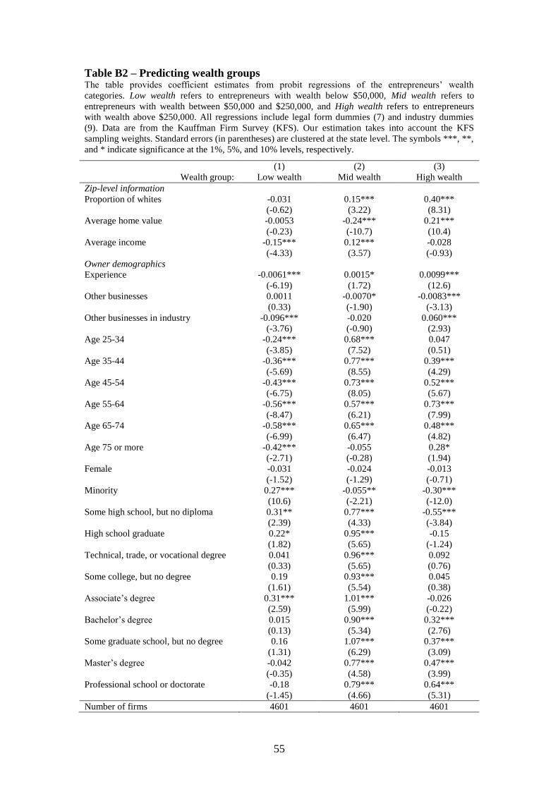
55
Table B2 – Predicting wealth groups The table provides coefficient estimates from probit regressions of the entrepreneurs’ wealth
categories. Low wealth refers to entrepreneurs with wealth below $50,000, Mid wealth refers to
entrepreneurs with wealth between $50,000 and $250,000, and High wealth refers to entrepreneurs
with wealth above $250,000. All regressions include legal form dummies (7) and industry dummies
(9). Data are from the Kauffman Firm Survey (KFS). Our estimation takes into account the KFS
sampling weights. Standard errors (in parentheses) are clustered at the state level. The symbols ***, **,
and * indicate significance at the 1%, 5%, and 10% levels, respectively.
(1) (2) (3)
Wealth group: Low wealth Mid wealth High wealth
Zip-level information
Proportion of whites -0.031 0.15*** 0.40***
(-0.62) (3.22) (8.31)
Average home value -0.0053 -0.24*** 0.21***
(-0.23) (-10.7) (10.4)
Average income -0.15*** 0.12*** -0.028
(-4.33) (3.57) (-0.93)
Owner demographics
Experience -0.0061*** 0.0015* 0.0099***
(-6.19) (1.72) (12.6)
Other businesses 0.0011 -0.0070* -0.0083***
(0.33) (-1.90) (-3.13)
Other businesses in industry -0.096*** -0.020 0.060***
(-3.76) (-0.90) (2.93)
Age 25-34 -0.24*** 0.68*** 0.047
(-3.85) (7.52) (0.51)
Age 35-44 -0.36*** 0.77*** 0.39***
(-5.69) (8.55) (4.29)
Age 45-54 -0.43*** 0.73*** 0.52***
(-6.75) (8.05) (5.67)
Age 55-64 -0.56*** 0.57*** 0.73***
(-8.47) (6.21) (7.99)
Age 65-74 -0.58*** 0.65*** 0.48***
(-6.99) (6.47) (4.82)
Age 75 or more -0.42*** -0.055 0.28*
(-2.71) (-0.28) (1.94)
Female -0.031 -0.024 -0.013
(-1.52) (-1.29) (-0.71)
Minority 0.27*** -0.055** -0.30***
(10.6) (-2.21) (-12.0)
Some high school, but no diploma 0.31** 0.77*** -0.55***
(2.39) (4.33) (-3.84)
High school graduate 0.22* 0.95*** -0.15
(1.82) (5.65) (-1.24)
Technical, trade, or vocational degree 0.041 0.96*** 0.092
(0.33) (5.65) (0.76)
Some college, but no degree 0.19 0.93*** 0.045
(1.61) (5.54) (0.38)
Associate’s degree 0.31*** 1.01*** -0.026
(2.59) (5.99) (-0.22)
Bachelor’s degree 0.015 0.90*** 0.32***
(0.13) (5.34) (2.76)
Some graduate school, but no degree 0.16 1.07*** 0.37***
(1.31) (6.29) (3.09)
Master’s degree -0.042 0.77*** 0.47***
(-0.35) (4.58) (3.99)
Professional school or doctorate -0.18 0.79*** 0.64***
(-1.45) (4.66) (5.31)
Number of firms 4601 4601 4601

56
Table C1 –Personal credit and Business credit Columns 1 and 4 replicate respectively the results from columns 2 and 5 in Table 4. Columns 2 and 5 control for different pre-trends across wealth groups, while columns 3
and 6 control for different trends across wealth groups. Pre-trend is a linear time trend that stops when a first change in exemptions occurs, after which point it takes the
value of zero. Trend is a linear time trend. Treated is a dummy that indicates whether the state passed an exemption law during our sample period. Low wealth refers to
entrepreneurs with wealth below $50,000, and High wealth refers to entrepreneurs with wealth above $250,000. All regressions include credit rating dummies. Data are from
the Kauffman Firm Survey (KFS) for the years 2004-2011. Our estimation takes into account the KFS sampling weights. Standard errors (in parentheses) are clustered at the
state level. The symbols ***, **, and * indicate significance at the 1%, 5%, and 10% levels, respectively.
Personal credit Business credit
(1) (2) (3) (4) (5) (6)
Exemptions ($1 million) -6.41** -5.51** -6.44** -1.36 -2.11 -1.61
(-2.33) (-1.97) (-2.24) (-0.64) (-1.06) (-0.75)
Exemptions LowWealth 8.56* 7.04 8.44 2.74 4.54 3.08
(1.67) (1.35) (1.56) (0.88) (1.61) (0.96)
Exemptions HighWealth 7.39** 6.60** 7.27** 0.41 0.91 0.47
(2.51) (2.16) (2.40) (0.13) (0.31) (0.15)
Pre-trend Treated -0.004 0.006
(-0.25) (0.52)
Pre-trend Treated LowWealth -0.008 0.001
(-0.36) (0.12)
Pre-trend Treated HighWealth 0.011 0.009
(0.70) (0.41)
Trend Treated 0.025* 0.007
(1.74) (0.69)
Trend Treated LowWealth -0.017 0.014*
(-1.29) (1.92)
Trend Treated HighWealth -0.012 -0.001
(-0.88) (-0.061)
Firm FE Yes Yes Yes Yes Yes Yes
Wealth group Year FE Yes Yes Yes Yes Yes Yes
State controls Yes Yes Yes Yes Yes Yes
Number of observations 30,318 30,318 30,318 30,318 30,318 30,318
R-squared 0.058 0.058 0.058 0.012 0.012 0.012
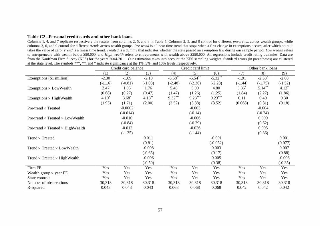
57
Table C2 –Personal credit cards and other bank loans Columns 1, 4, and 7 replicate respectively the results from columns 2, 5, and 8 in Table 5. Columns 2, 5, and 8 control for different pre-trends across wealth groups, while
columns 3, 6, and 9 control for different trends across wealth groups. Pre-trend is a linear time trend that stops when a first change in exemptions occurs, after which point it
takes the value of zero. Trend is a linear time trend. Treated is a dummy that indicates whether the state passed an exemption law during our sample period. Low wealth refers
to entrepreneurs with wealth below $50,000, and High wealth refers to entrepreneurs with wealth above $250,000. All regressions include credit rating dummies. Data are
from the Kauffman Firm Survey (KFS) for the years 2004-2011. Our estimation takes into account the KFS sampling weights. Standard errors (in parentheses) are clustered
at the state level. The symbols ***, **, and * indicate significance at the 1%, 5%, and 10% levels, respectively.
Credit card balance Credit card limit Other bank loans
(1) (2) (3) (4) (5) (6) (7) (8) (9)
Exemptions ($1 million) -2.30 -1.69 -2.10 -5.58** -5.54** -5.32** -1.91 -2.53* -2.08
(-1.16) (-0.81) (-1.03) (-2.48) (-2.36) (-2.28) (-1.44) (-1.75) (-1.52)
Exemptions LowWealth 2.47 1.05 1.76 5.48 5.00 4.80 3.86* 5.14** 4.12*
(0.68) (0.27) (0.47) (1.47) (1.26) (1.25) (1.84) (2.27) (1.86)
Exemptions HighWealth 4.10* 3.68* 4.13** 9.32*** 9.23*** 9.23*** 0.11 0.49 0.30
(1.93) (1.71) (2.00) (3.52) (3.38) (3.52) (0.068) (0.31) (0.18)
Pre-trend Treated -0.0002 -0.003 -0.004
(-0.014) (-0.14) (-0.24)
Pre-trend Treated LowWealth -0.010 -0.006 0.009
(-0.84) (-0.29) (0.62)
Pre-trend Treated HighWealth -0.012 -0.026 0.005
(-1.25) (-1.44) (0.36)
Trend Treated 0.011 -0.001 0.001
(0.81) (-0.052) (0.077)
Trend Treated LowWealth -0.008 0.003 0.007
(-0.65) (0.17) (0.88)
Trend Treated HighWealth -0.006 0.005 -0.003
(-0.50) (0.38) (-0.35)
Firm FE Yes Yes Yes Yes Yes Yes Yes Yes Yes
Wealth group year FE Yes Yes Yes Yes Yes Yes Yes Yes Yes
State controls Yes Yes Yes Yes Yes Yes Yes Yes Yes
Number of observations 30,318 30,318 30,318 30,318 30,318 30,318 30,318 30,318 30,318
R-squared 0.043 0.043 0.043 0.068 0.068 0.068 0.042 0.042 0.042
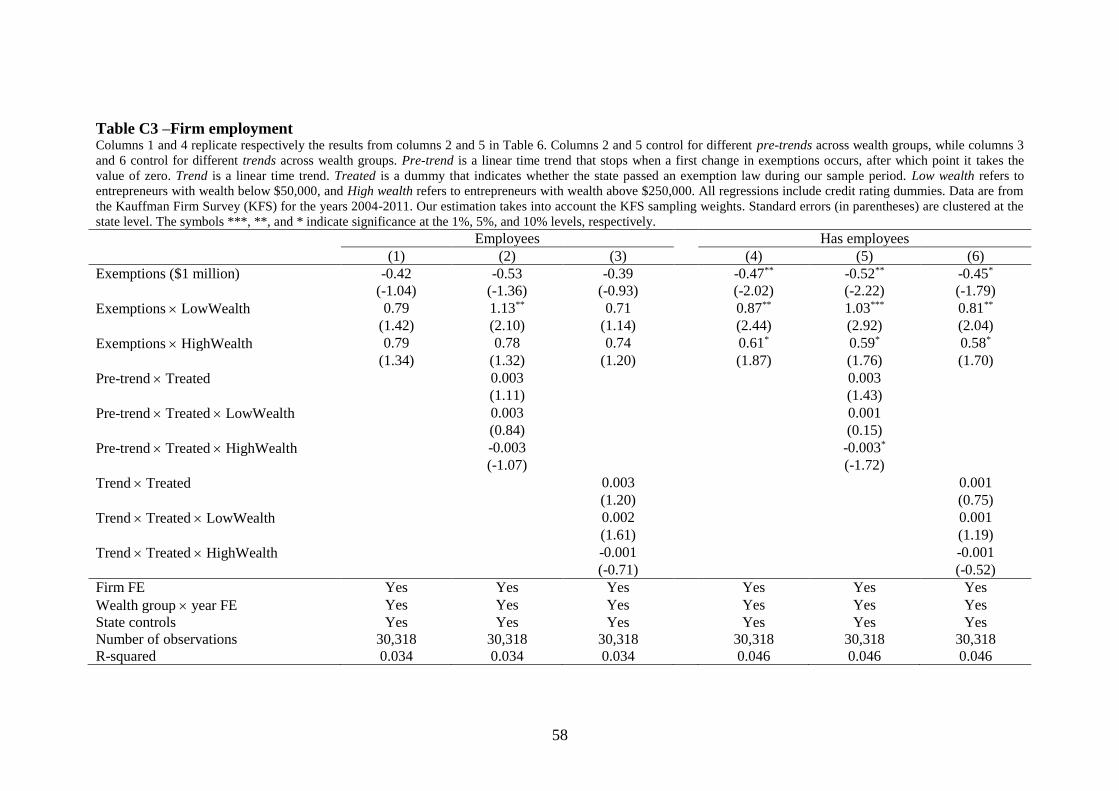
58
Table C3 –Firm employment Columns 1 and 4 replicate respectively the results from columns 2 and 5 in Table 6. Columns 2 and 5 control for different pre-trends across wealth groups, while columns 3
and 6 control for different trends across wealth groups. Pre-trend is a linear time trend that stops when a first change in exemptions occurs, after which point it takes the
value of zero. Trend is a linear time trend. Treated is a dummy that indicates whether the state passed an exemption law during our sample period. Low wealth refers to
entrepreneurs with wealth below $50,000, and High wealth refers to entrepreneurs with wealth above $250,000. All regressions include credit rating dummies. Data are from
the Kauffman Firm Survey (KFS) for the years 2004-2011. Our estimation takes into account the KFS sampling weights. Standard errors (in parentheses) are clustered at the
state level. The symbols ***, **, and * indicate significance at the 1%, 5%, and 10% levels, respectively.
Employees Has employees
(1) (2) (3) (4) (5) (6)
Exemptions ($1 million) -0.42 -0.53 -0.39 -0.47** -0.52** -0.45*
(-1.04) (-1.36) (-0.93) (-2.02) (-2.22) (-1.79)
Exemptions LowWealth 0.79 1.13** 0.71 0.87** 1.03*** 0.81**
(1.42) (2.10) (1.14) (2.44) (2.92) (2.04)
Exemptions HighWealth 0.79 0.78 0.74 0.61* 0.59* 0.58*
(1.34) (1.32) (1.20) (1.87) (1.76) (1.70)
Pre-trend Treated 0.003 0.003
(1.11) (1.43)
Pre-trend Treated LowWealth 0.003 0.001
(0.84) (0.15)
Pre-trend Treated HighWealth -0.003 -0.003*
(-1.07) (-1.72)
Trend Treated 0.003 0.001
(1.20) (0.75)
Trend Treated LowWealth 0.002 0.001
(1.61) (1.19)
Trend Treated HighWealth -0.001 -0.001
(-0.71) (-0.52)
Firm FE Yes Yes Yes Yes Yes Yes
Wealth group year FE Yes Yes Yes Yes Yes Yes
State controls Yes Yes Yes Yes Yes Yes
Number of observations 30,318 30,318 30,318 30,318 30,318 30,318
R-squared 0.034 0.034 0.034 0.046 0.046 0.046

59
Table C4 –Firm revenue and efficiency Columns 1 and 4 replicate respectively the results from columns 2 and 5 in Table 7. Columns 2 and 5 control for different pre-trends across wealth groups, while columns 3
and 6 control for different trends across wealth groups. Pre-trend is a linear time trend that stops when a first change in exemptions occurs, after which point it takes the
value of zero. Trend is a linear time trend. Treated is a dummy that indicates whether the state passed an exemption law during our sample period. Low wealth refers to
entrepreneurs with wealth below $50,000, and High wealth refers to entrepreneurs with wealth above $250,000. All regressions include credit rating dummies. Data are from
the Kauffman Firm Survey (KFS) for the years 2004-2011. Our estimation takes into account the KFS sampling weights. Standard errors (in parentheses) are clustered at the
state level. The symbols ***, **, and * indicate significance at the 1%, 5%, and 10% levels, respectively.
Generate revenue Efficiency
(1) (2) (3) (4) (5) (6)
Exemptions ($1 million) -0.66*** -0.67*** -0.68*** -3.26*** -3.78*** -3.50***
(-2.88) (-3.19) (-3.13) (-3.39) (-4.05) (-3.92)
Exemptions LowWealth 1.21*** 1.22*** 1.28*** 5.87*** 7.08*** 6.33***
(3.19) (3.41) (3.47) (3.90) (4.73) (4.40)
Exemptions HighWealth 0.26 0.30 0.27 1.76 2.01 1.88
(0.73) (0.85) (0.77) (1.28) (1.51) (1.44)
Pre-trend Treated 0.0003 0.009
(0.098) (0.95)
Pre-trend Treated LowWealth -0.005** -0.027***
(-2.01) (-2.94)
Pre-trend Treated HighWealth 0.001 -0.002
(0.33) (-0.19)
Trend Treated -0.001 0.002
(-1.14) (0.40)
Trend Treated LowWealth 0.001 0.013**
(1.11) (3.83)
Trend Treated HighWealth 0.001 -0.002
(1.09) (-0.43)
Firm FE Yes Yes Yes Yes Yes Yes
Wealth group year FE Yes Yes Yes Yes Yes Yes
State controls Yes Yes Yes Yes Yes Yes
Number of observations 30,318 30,318 30,318 30,318 30,318 30,318
R-squared 0.323 0.323 0.323 0.277 0.277 0.277

60
Table D1 –Personal credit and Business credit Columns 1 and 3 replicate respectively the results from columns 1 and 4 in Table 4, in which standard
errors were clustered at the state level. Columns 2 and 4 re-estimate the regressions with jackknifed
standard errors. Data are from the Kauffman Firm Survey (KFS) for the years 2004-2011. Our
estimation takes into account the KFS sampling weights. The symbols ***, **, and * indicate
significance at the 1%, 5%, and 10% levels, respectively.
Personal credit (log) Business credit (log)
Standard errors:
(1)
Clustered
(2)
Jackknifed
(3)
Clustered
(4)
Jackknifed
Exemptions
Exemptions ($1 million) -5.66** -5.66** -2.20 -2.20
(-2.08) (-2.06) (-1.12) (-1.04)
Exemptions LowWealth 7.38 7.38* 4.56 4.56
(1.48) (1.69) (1.64) (1.55)
Exemptions HighWealth 6.60** 6.60* 0.85 0.85
(2.20) (1.94) (0.29) (0.30)
Firm controls 1.19*** 1.19*** 0.88*** 0.88***
Credit risk 1 (5.13) (5.02) (5.81) (4.20)
0.98*** 0.98*** 0.48*** 0.48***
Credit risk 2 (6.70) (7.43) (5.67) (5.10)
0.81*** 0.81*** 0.41*** 0.41***
Credit risk 3 (7.35) (7.44) (6.68) (5.58)
0.48*** 0.48*** 0.22*** 0.22**
Credit risk 4 (4.21) (3.54) (3.83) (2.57)
-0.10 -0.10 0.081 0.081
Credit risk 5 (-0.64) (-0.68) (0.89) (0.79)
Firm FE Yes Yes Yes Yes
Year FE Yes Yes Yes Yes
State controls Yes Yes Yes Yes
Number of observations 30,318 30,318 30,318 30,318
R-squared 0.058 0.058 0.011 0.011

61
Table D2 – Credit cards and Other bank loans Columns 1, 3, and 5 replicate respectively the results from columns 1, 4, and 7 in Table 5, in which standard errors were clustered at the state level. Columns 2, 4, and 6 re-
estimate the regressions with jackknifed standard errors. Data are from the Kauffman Firm Survey (KFS) for the years 2004-2011. Our estimation takes into account the KFS
sampling weights. The symbols ***, **, and * indicate significance at the 1%, 5%, and 10% levels, respectively.
Credit card balance (log) Credit card limit (log) Other bank loans (log)
Standard errors:
(1)
Clustered
(2)
Jackknifed
(3)
Clustered
(4)
Jackknifed
(5)
Clustered
(6)
Jackknifed
Exemptions ($1 million) -1.70 -1.70 -5.39** -5.39** -2.45* -2.45
(-0.84) (-0.82) (-2.32) (-2.05) (-1.77) (-1.48)
Exemptions LowWealth 1.20 1.20 4.93 4.93 4.97** 3.86**
(0.32) (0.37) (1.29) (1.25) (2.30) (2.03)
Exemptions HighWealth 3.83* 3.83 9.41*** 9.41*** 0.42 0.42
(1.80) (1.48) (3.49) (2.86) (0.25) (0.19)
Firm controls
Credit risk 1 0.27** 0.27* 0.27* 0.27 0.10 0.10
(2.63) (1.78) (1.94) (1.47) (0.63) (0.57)
Credit risk 2 0.34*** 0.34*** 0.37*** 0.37*** 0.28*** 0.28***
(3.94) (3.52) (3.13) (3.27) (3.40) (2.94)
Credit risk 3 0.32*** 0.32*** 0.35*** 0.35*** 0.24*** 0.24***
(5.26) (3.92) (3.30) (3.48) (3.55) (3.12)
Credit risk 4 0.28*** 0.28*** 0.30*** 0.30** 0.13* 0.13
(3.12) (2.72) (3.12) (2.50) (1.98) (1.44)
Credit risk 5 -0.21* -0.21* -0.19 -0.19 -0.0079 -0.0079
(-1.78) (-1.75) (-1.37) (-1.36) (-0.080) (-0.073)
Firm FE Yes Yes Yes Yes Yes Yes
Year FE Yes Yes Yes Yes Yes Yes
State controls Yes Yes Yes Yes Yes Yes
Number of observations 30,318 30,318 30,318 30,318 30,318 30,318
R-squared 0.042 0.042 0.067 0.067 0.041 0.041

62
Table D3 – Firm employment Columns 1 and 3 replicate respectively the results from columns 1 and 4 in Table 6, in which standard
errors were clustered at the state level. Columns 2 and 4 re-estimate the regressions with jackknifed
standard errors. Data are from the Kauffman Firm Survey (KFS) for the years 2004-2011. Our
estimation takes into account the KFS sampling weights. The symbols ***, **, and * indicate
significance at the 1%, 5%, and 10% levels, respectively.
Employees (log) Has employees (0/1)
Standard errors:
(1)
Clustered
(2)
Jackknifed
(3)
Clustered
(4)
Jackknifed
Exemptions
Exemptions ($1 million) -0.49 -0.49 -0.51** -0.51**
(-1.25) (-1.02) (-2.17) (-2.09)
Exemptions LowWealth 1.01* 1.01 0.99*** 0.99**
(1.86) (1.29) (2.78) (2.50)
Exemptions HighWealth 0.77 0.77 0.60* 0.60*
(1.31) (1.28) (1.78) (1.92)
Firm controls 0.27*** 0.27*** 0.14*** 0.14***
Credit risk 1 (9.24) (7.63) (8.97) (7.17)
0.19*** 0.19*** 0.10*** 0.10***
Credit risk 2 (9.42) (9.26) (9.16) (8.35)
0.12*** 0.12*** 0.066*** 0.066***
Credit risk 3 (7.43) (6.76) (7.31) (6.10)
0.082*** 0.082*** 0.048*** 0.048***
Credit risk 4 (4.44) (4.05) (3.71) (3.69)
0.00081 0.00081 0.012 0.012
Credit risk 5 (0.046) (0.031) (1.06) (0.80)
Firm FE Yes Yes Yes Yes
Year FE Yes Yes Yes Yes
State controls Yes Yes Yes Yes
Number of observations 30,318 30,318 30,318 30,318
R-squared 0.033 0.033 0.045 0.045

63
Table D4 – Firm revenue and efficiency Columns 1 and 3 replicate respectively the results from columns 1 and 4 in Table 7, in which standard
errors were clustered at the state level. Columns 2 and 4 re-estimate the regressions with jackknifed
standard errors. Data are from the Kauffman Firm Survey (KFS) for the years 2004-2011. Our
estimation takes into account the KFS sampling weights. The symbols ***, **, and * indicate
significance at the 1%, 5%, and 10% levels, respectively.
Generate revenue (0/1) Efficiency (log)
Standard errors:
(1)
Clustered
(2)
Jackknifed
(3)
Clustered
(4)
Jackknifed
Exemptions
Exemptions ($1 million) -0.73*** -0.73*** -4.08*** -4.08***
(-3.55) (-3.30) (-4.37) (-4.20)
Exemptions LowWealth 1.36*** 1.36*** 7.69*** 7.69***
(3.88) (3.78) (5.06) (5.05)
Exemptions HighWealth 0.33 0.33 2.18 2.18*
(0.96) (1.18) (1.64) (1.85)
Firm controls 0.094*** 0.094*** 0.42*** 0.42***
Credit risk 1 (5.29) (4.77) (4.93) (4.66)
0.067*** 0.067*** 0.29*** 0.29***
Credit risk 2 (5.76) (5.27) (6.14) (5.74)
0.058*** 0.058*** 0.27*** 0.27***
Credit risk 3 (6.10) (5.32) (7.32) (6.48)
0.055*** 0.055*** 0.16*** 0.16***
Credit risk 4 (6.55) (4.09) (4.39) (3.11)
0.047*** 0.047*** 0.21*** 0.21***
Credit risk 5 (3.04) (3.19) (3.97) (3.65)
Firm FE Yes Yes Yes Yes
Year FE Yes Yes Yes Yes
State controls Yes Yes Yes Yes
Number of observations 30,318 30,318 30,318 30,318
R-squared 0.323 0.323 0.277 0.277

64
Table D5 – Firm survival Column 1 replicates the results from Table 8, in which standard errors were
clustered at the state level. Column 2 re-estimate the regression with jackknifed
standard errors. Data are from the Kauffman Firm Survey (KFS) for the years 2004-
2011. Our estimation takes into account the KFS sampling weights. The symbols
***, **, and * indicate significance at the 1%, 5%, and 10% levels, respectively.
Bankruptcy (0/1)
Standard errors: (1)
Clustered
(2)
Jackknifed
Exemptions
Exemptions ($1 million) 2.75*** 2.75**
(2.87) (2.00)
Exemptions LowWealth -2.86* -2.86
(-1.80) (-1.38)
Exemptions HighWealth -2.09* -2.09
(-1.66) (-1.14)
Firm controls
Credit risk 1 -1.87*** -1.87***
(-11.8) (-8.61)
Credit risk 2 -1.40*** -1.40***
(-15.0) (-15.8)
Credit risk 3 -0.98*** -0.98***
(-16.6) (-15.1)
Credit risk 4 -0.83*** -0.83***
(-12.9) (-9.59)
Credit risk 5 -0.46*** -0.46***
(-5.50) (-5.24)
State fixed effects Yes Yes
State controls Yes Yes
Owner controls Yes Yes
Firm controls Yes Yes
Number of observations 30,318 30,318

65
Table E1 – Bank financing: Personal credit and Business credit The table displays coefficients from panel regressions of the log of one plus the dollar
amounts of Personal credit and Business credit. Age<4 and Age≥4 indicate respectively
whether the observation is before or after 2008. Exemptions is the sum of the homestead
exemption and the personal property exemptions, which includes the following assets:
jewelry, motor vehicles, cash and deposits, and the wildcard exemption. Exemption values are
in million of dollars. Low wealth refers to entrepreneurs with wealth below $50,000, and High
wealth refers to entrepreneurs with wealth above $250,000. Data are from the Kauffman Firm
Survey (KFS) for the years 2004-2011. Our estimation takes into account the KFS sampling
weights. Standard errors (in parentheses) are clustered at the state level. The symbols ***, **,
and * indicate significance at the 1%, 5%, and 10% levels, respectively.
Personal credit
(log)
Business credit
(log)
(1) (2)
Exemptions
Exemptions (Age < 4) -7.49** 1.58
(-2.59) (0.81)
Exemptions (Age ≥ 4) -5.17* -2.89
(-1.92) (-1.38)
Exemptions LowWealth (Age < 4) 10.94** -0.66
(2.15) (-0.21)
Exemptions LowWealth (Age ≥ 4) 6.60 5.51*
(1.35) (1.89)
Exemptions HighWealth (Age < 4) 6.21 -3.41
(1.52) (-1.35)
Exemptions HighWealth (Age ≥ 4) 6.60** 1.51
(2.17) (0.50)
Credit rating Dummies Yes Yes
Firm FE Yes Yes
Year FE No Yes
State controls No Yes
Number of observations 30,318 30,318
R-squared 0.058 0.011