HOW DOES THE

POLARITY OF ORGANIC

SOLVENTS AFFECT TO

THE PARTITION

COEFFICIENT OF

CAFFEINE BETWEEN THE

ORGANIC SOLVENT AND

WATER?

María del Mar Castro Orta SEVILLA, 5TH MARCH 2012 Words: 3293

1

Abstract

The objective of the investigation is to determine polarity index influence on partition

coefficient of caffeine between water and five different organic solvents not miscible with

water at two different temperatures.

In order to achieve this, an aqueous solution of caffeine was mixed with the same volume

of each organic solvent in a closed flask and equilibrium was let to establish, first at room

temperature and later at 80 ºC. Partition coefficient is determined by measuring the variation

of concentration of caffeine in the aqueous phase by UV-VIS spectroscopy.

After doing the investigation, we can state that polarity index of the organic solvents does

affect to the partition coefficient, hence, to its caffeine solubilities. As the polarity index

increase, so does the partition coefficient, which means that caffeine solubility at the organic

solvent increases. However, temperature does not cause a clear effect on the partition

coefficient, it depends on the nature of each organic solvent.

Number of words: 155.

2

INDEX

1. Introduction……………………………………………………………………………………………………………………….3

2. Variables…………………………………………………………………………………………………………………………….5

3. Equipment and procedure…………………………………………………………………………………………………5

3.1. Equipment……………..……………………………………………………………………….………………………….5

3.2. Substances…………………………………………………………………………………………………………………5

3.3. Procedure…………………………………………………………………………………………………………………..5

3.3.1. Spectrum of caffeine…………………………………………………………………………………………..6

3.3.2. Calibration…………………………………………………………………………………………………………..6

3.3.3. Measurements of the concentration of caffeine in different solvents…………….…6

4. Results……………………………………………………………………………………………………………………………….7

4.1. Determination of the suitable wavelength in caffeine spectrum…………………………….…7

4.2. Calibration………………………………………………………………………………………………………………….8

4.3. Experimental measurements……………………………………………………………………………………..9

5. Discussion………………………………………………………………………………………………………………….….…12

5.1. Conclusion………………………………………………………………………………………………………………..12

5.2. Procedure evaluation……………………………………………………………………………………………….12

5.3. Investigation improvements……………………………………………………………………………………..14

6. Bibliography……………………………………………………………………………………………………………………..15

3

1. Introduction

Caffeine is the ordinary name for 1,3,7-trimethylxanthine, with the molecular structure of figure 1.1(8). Numerous plants naturally produce this chemical, it occurs in coffee, tea, guarana, kola nuts, maté and cacao. It has significant effects in human beings because it stimulates the central nervous system, heart, blood vessels and kidneys; it also behaves as a mild diuretic.

Pure caffeine is a bitter white powder which has a melting point at 238˚C, it sublimates at 178˚C at atmospheric pressure. Caffeine is less soluble in organic compounds than in hot water. Hence, there will be a relation between organic compounds and caffeine solubility.

Polarities of organic compounds may guide the solubility pattern. Polarity depends on the electronegativity difference between atoms in a bond, the greater the difference, the more polar the bond; and on the geometry of the whole molecule. This feature must be analyzed with the solubility in water as immiscible compounds must be used. The data has been obtained from a website (6) about chemical ecology, which we can see below:

Solvent Polarity Index Solubility in Water (%)

Hexane 0 0.001

Cyclohexane 0.2 0.01

Carbon tetrachloride 1.6 0.08

Benzene 2.7 0.18

Chloroform 4.1 0.815

The variable that I'm going to study is the partition coefficient (kc). Considering a substance that can be dissolved in two different solvents that cannot be mixed together, we can find a relationship between the concentrations of this substance in both solvents. This relationship is expressed by the partition coefficient:

I will study the partition coefficient of caffeine between five different organic solvents and water. When caffeine solution in water gets in contact with any solvent, surfaces of both liquids which are in contact interact. This interaction is to transfer a certain amount of caffeine dissolved in water to the new solvent. The transfer continues until equilibrium is reached, known as partition equilibrium. Therefore, the following equilibrium represents the reaction we will work on:

Concentration can be studied by various methods. Gravimetric analysis, for example, determines quantitatively the amount of analyte based on the mass of a solid. Volumetric analysis can also provide concentration information of a solution. A known concentration and

Figure 1.1.: The

molecular structure

of caffeine

4

volume of reagent reacts with a solution of analyte to determine concentration, this is also known as titration. Spectroscopy is a common quantitative method to determine unknown concentrations, in my case, UV-VIS spectrometer was used; hence, I have needed a deeper understanding of the analytical technique. Thus, expanding the knowledge on this topic with the book of Analytical Chemistry (3) has allowed me to understand in greater depth the function of the UV-VIS spectrometer and data processing explained in later sections.

Organic chemistry had been an important chapter in those years. We had been working on a deep knowledge in this field, which developed my great interest. Therefore, I focused my first overview in this area. In addition, caffeine studies and its biological repercussions attract strongly my attention. Investigating about both paths simultaneously guided me to different chemical aspects relationing those concepts. The blending between the investigations about caffeine and the partition coefficient has guided me to the following research question:

How the polarity of different organic compounds does affects to the partition coefficient between the caffeine concentration and the caffeine dissolution?

The objective was to find a conclusion about the trend, if any, of the partition coefficient of caffeine depending on the polarity of organic solvents. Additionally, the variable has been studied in two different temperatures, obtaining a broader vision of the investigation.

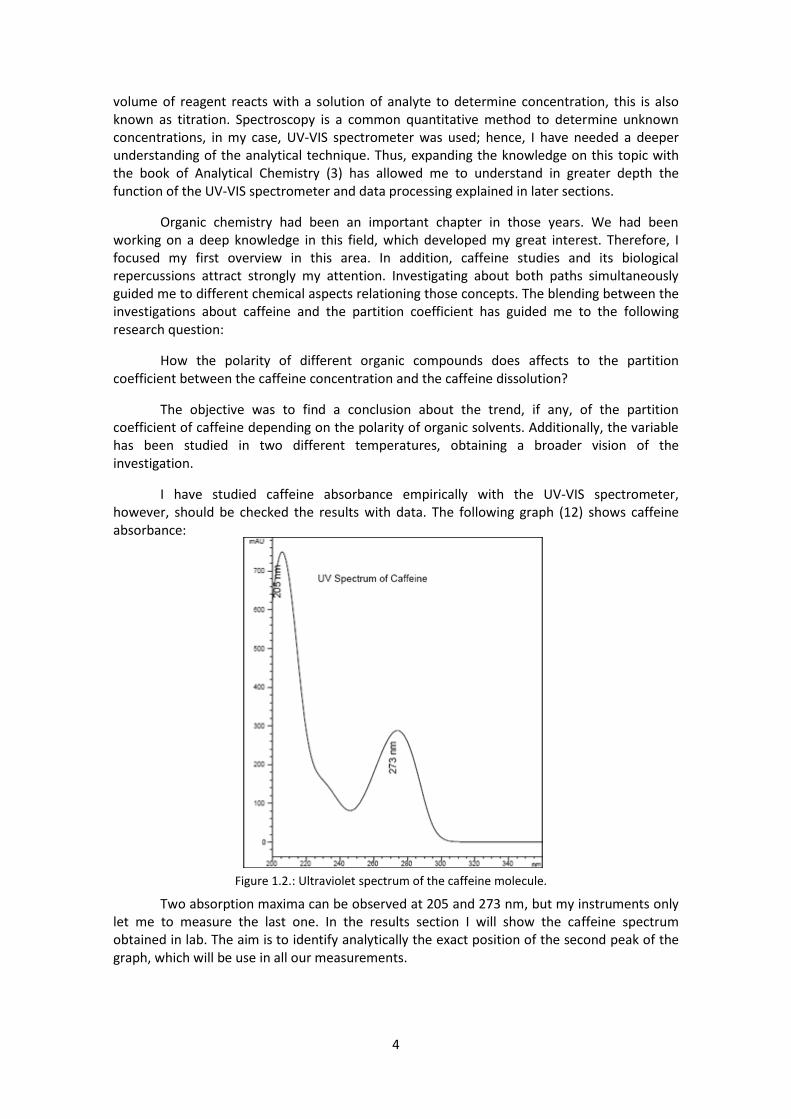
I have studied caffeine absorbance empirically with the UV-VIS spectrometer, however, should be checked the results with data. The following graph (12) shows caffeine absorbance:

Two absorption maxima can be observed at 205 and 273 nm, but my instruments only let me to measure the last one. In the results section I will show the caffeine spectrum obtained in lab. The aim is to identify analytically the exact position of the second peak of the graph, which will be use in all our measurements.

Figure 1.2.: Ultraviolet spectrum of the caffeine molecule.

5

2. Variables

The independent variable is the polarity index of the different organic solvents which will establish the equilibrium of caffeine concentration with water. Therefore, five solvents will be used: cyclohexane, carbon tetrachloride, benzene, chloroform and hexane. In addition, the temperature is an independent variable as well. Two series at different temperatures, room temperature and 80˚C, using those solvents, will be completed.

The dependent variable is the partition coefficient, Kc, depending on the ratio of caffeine concentration between water and organic solvents.

Controlled variables should be taken into account. Initial caffeine concentration in water is 2.5·10-5M, which is essential to maintain it constant at it will be necessary to obtain Kc. Both water and organic solvents volumes must be equal when they are mixed. In research, 10mL of each liquid will be used. Moreover, organic solvents purity, which is shown in equipment section, has been supervised as it can vaguely affect results. The peak of the caffeine absorbance graph determines the suitable wavelength for UV-VIS spectrometer analysis in order to obtain the corresponding absorbance of each equilibrium sample. Finally, pressure should be controlled in the entire procedure in order to reduce every possible source of error.

3. Equipment and procedure

3.1. Equipment

- UV-Visible, Scanning Spectrophotometer (Miton Roy Spectronic 1001 Plus)

- Sample holder

- Plastic pipette

- Pipette

- Pipette bulb

- Volumetric flask

o 1unit - 1L

o 6 units – 50mL

- 5 separatory funnels

- Water bath

- Thermometer

3.2. Substances

- Cyclohexane, purity of 100%, Scharlau.

- Carbon tetrachloride, purity of 100%, Panreac.

- Benzene for analysis, purity of 99%, Panreac.

- Chloroform stabilized with ethanol, purity of 99,0%, Panreac.

- Hexane, mixture of alkanes, Scharlau.

- Acetone

- Distilled H2O

- Caffeine powder

3.3. Procedure

- Prepare a caffeine dissolution 2.5·10-5M in a volumetric flask of 1 liter.

- Operation of spectrophotometer.

6

3.3.1. Spectrum of caffeine

- Pour dissolution of caffeine2.5·10-5 M in one of the sample holder until the

mark that is in it with the plastic pipette.

- In the other sample holder, add distilled water to use as reference in the

scanning spectrophotometer.

- Turn on the scanning spectrophotometer, and notify the distilled water as

reference.

- Measure the absorbance for different wavelengths (λ). Start at 190 nm and

end at 350 nm, measure every 5 nm.

- Look at the maximum absorbance and repeat the analysis for wavelengths

close to it every 2 nm.

- Identify the maximum absorbance; we will work with it during the

investigation.

3.3.2. Calibration

The calibration curve is an analytical chemistry method used to measure the concentration of

a substance in a sample by comparison with a number of elements of known concentration. It

is based on the existence of a mathematical relationship between a character principle

measurable, absorbance spectrophotometry, and the concentration. It will be require the

calibration curve to determine the concentration of caffeine in different solvents through its

absorbance.

- Prepare seven solutions of caffeine with different concentrations, using the

initial solution of 2.5·10-5 M.

o 2.50·10-5 M

o 2.00·10-5 M

o 1.25·10-5 M

o 1.00·10-5 M

o 6.25·10-6 M

o 5.00·10-6 M

o 3.13·10-6 M

- Turn on the scanning spectrophotometer

- Pour distilled water in one of the sample holder.

- Place the distilled water as absorbance 0.

- Measure the absorbance of the 7 solutions.

- Analyze the relation between the concentration and the absorbance by a

mathematical function.

3.3.3. Measurements of the concentration of caffeine in different solvents.

- Clean 5 separatory funnels with acetone and let them air dry.

- Pour 10mL of the caffeine dissolution 2.5·10-5 M in each separatory funnel

using a pipette.

- Pour 10mL of hexane in separatory funnel 1 with a clean pipette.

- Stir it for five minutes.

7

- Repeat the process with the other 4 organic solvents.

- Knowing the density of each solvent (13), we know where the caffeine

dissolution is situated. The absorbance of aqueous phase will be measured as

some organic solvents are slightly miscible in water. Add it to one sample

holder at room temperature (having as reference distilled water in the

scanning spectrophotometer) and measure it absorbance.

Solvent Density (g/cm3)

Hexane 0.655

Cyclohexane 0.779

Carbon tetrachloride 1.595

Benzene 0.878

Chloroform 1.483

- Heat the separatory funnels at 80 ºC in a water bath and a thermometer. - Pour the caffeine dissolution 2.5·10-5 M of separatory funnel 1 in the sample

holder and measure it absorbance. (Remember that we know the caffeine dissolution position because the densities of the different solvents.)

- Repeat the previous step with separatory funnels 2, 3, 4 and 5.

4. Results

4.1. Determination of the suitable wavelength in caffeine spectrum.

Finding the wavelength where caffeine has a significantly high absorbance will increase

the accuracy of results, so the peak in the Graph 1 is more sensible to be detected for

followings measurements.

GRAPH 1: Caffeine Absorbance

0

0.5

1

1.5

2

2.5

3

220 240 260 280 300 320 340 360

Ab

sorb

ance

Wavelength (nm)

Caffeine Absorbance

8

4.2. Calibration

A calibration curve is necessary in order to obtain caffeine concentration as it represents the relationship between both variables. Measuring absorbance of several known concentrations of caffeine in water will give us the graphic relationship.

Absorbance has the spectrometer own error, which is ±0,001 in every sample. As it error bars are negligible due to the Y axis scale, they will be omitted. Concentration, however, carries an analyzable error which comes from the method followed. Therefore, each sample has its own error represented in graph 2.

TABLE 1: Calibration curve

Concentration (M) Absorbance

(±0.001)

2.50·10-5±5·10-7 2.419

2.00·10-5±7·10-7 1.927

1.25·10-5±5·10-7 1.219

1.00·10-5±5·10-7 1.027

6.3·10-6±4·10-7 0.624

5.0·10-6±4·10-7 0.486

3.1·10-6±3·10-7 0.315

GRAPH 2: Calibration curve

The equation of the calibration curve is:

0

0.5

1

1.5

2

2.5

3

0.00E+00 5.00E-06 1.00E-05 1.50E-05 2.00E-05 2.50E-05 3.00E-05

Ab

sorb

ance

Concentration (mol·L-1)

Calibration curve

9

Once I reach a mathematical expression relating absorbance and caffeine concentration in

water, it is possible to recognize any caffeine concentration from a known absorbance.

4.3. Experimental measurements

TABLE 2: Solvents’ absorbances

Solvent Polarity

Index Absorbance of aqueous phase at

room temperature (±0.001) Absorbance of aqueous phase at 80 ˚C (±0.001)

Hexane 0 2.418 2.412

Cyclohexane 0.2 2.414 2.410

Carbon tetrachloride

1.6 2.028 1.999

Benzene 2.7 1.418 1.686

Chloroform 4.1 1.341 1.555

Calculations of the partition coefficient

The ratio between both concentrations of caffeine can be measured by the following formula:

I determine the ratio between the concentrations in Organic solvent /H2O. Defining this ratio will indicate the proportion of caffeine concentration in water between different organic solvents, hence, if Kc>1, the caffeine concentration in the organic solvent is higher than the one in water; if Kc=1, both concentrations are equals; if Kc<1, the caffeine concentration in water is higher than the one in organic solvent. In addition, caffeine relative solubilities in different solvents will be identified due to Kc. Empirically, we measure water absorbance once reached the following equilibrium:

Previously, we have made the calibration curve showing the relation between absorbance and concentration in caffeine. Therefore, once the corresponding absorbance is known, I can obtain its concentration through graph 2.

We need both caffeine concentrations, in water as well as in the organic solvent. Caffeine concentration in water is already explained as we get it directly from data; however, as we have used the same volumes of both aqueous and organic phase, and no significant solubility in water of any of the organic solvent used in the study exists, the concentration in the organic solvent is obtained through the difference between the initial caffeine concentration and the new one in water after the equilibrium.

10

TABLE 3: Partition coefficients at room temperature and 80 ˚C.

Solvent Polarity

Index

Concentration of aqueous phase at

room temperature (M x

105)

Concentration of aqueous phase

at 80˚C (M x 105)

Kc at room temperature

Kc at 80˚C

Hexane 0 2.49±0.02 2.48±0.02 0.006±0.03 0.008±0.03

Cyclohexane 0.2 2.48±0.02 2.48±0.02 0.008±0.03 0.008±0.03

Carbon tetrachloride

1.6 2.08±0.01 2.05±0.01 0.20±0.03 0.22±0.03

Benzene 2.7 1.46±0.01 1.73±0.01 0.72±0.05 0.45±0.04

Chloroform 4.1 1.38±0.01 1.60±0.01 0.81±0,05 0.56±0,04

The relation between Kc and the polarity index is graphed is Graph 3 at room

temperature, and in Graph 4 at 80 ˚C. In order to observe clearly the relation between both

variables, I have decided to use a logarithm scale in the Y axis.

GRAPH 3: Kc vs Polarity index at room temperature.

A linear relation between the polarity index and Kc at room temperature can be found:

1.00E-04

1.00E-03

1.00E-02

1.00E-01

1.00E+00

0 0.5 1 1.5 2 2.5 3 3.5 4 4.5

Par

titi

on

co

eff

icie

nt

Polarity index

Kc vs Polarity index at room temperature

11

GRAPH 4: Kc vs Polarity index at 80˚C.

At 80 ˚C, a similar relation is found:

To compare both patterns we should observe both temperatures results in a single graph:

GRAPH 3: Kc vs. polarity index at room temperature and at 80˚C.

It is not possible to determine a constant temperature influence to partition coefficient as it varies between organic solvents samples.

1.00E-03

1.00E-02

1.00E-01

1.00E+00

0 0.5 1 1.5 2 2.5 3 3.5 4 4.5

Par

titi

on

co

ffic

ien

t

Polarity index

Kc vs Polarity index at 80 ˚C

1.00E-04

1.00E-03

1.00E-02

1.00E-01

1.00E+00

0 0.5 1 1.5 2 2.5 3 3.5 4 4.5

Par

titi

on

co

ffic

ien

t

Polarity index

Kc vs Polarity index

80ºC

Room temperature

12

5. Discussion

5.1. Conclusions

The polarity of the organic solvents chosen affects the partition coefficient. As the polarity index increases, Kc increases. They are directly proportional because they do represent an increasing linear relation graphically, represented by a linear function. It is possible to state an increasing order of solubility of the compounds used:

Hexane<Cyclohexane<Carbon tetrachloride<Benzene<Chloroform<Water

Bearing in mind the partition coefficient expression:

It is possible to deduce the relative caffeine solubility in the organic solvent linked to its polarity; hence, as the polarity index increases and so does Kc, the caffeine concentration in the organic solvent increases too, thus rising its solubility qualitatively.

Analyzing temperature variable, partition coefficient at 80 ˚C and room temperature does not show a clear variation, it depends on the organic solvent. Taking into account the equilibrium established:

Regarding equilibrium enthalpies, according to le Chatelier’s principle1, increasing the temperature of the equilibrium will change the position of it to minimize this change. If Kc increases with temperature the forward rate of equilibrium is endothermic because the position of equilibrium has been displaced to the right as caffeine concentration in the organic solvent increases. In contrast, if Kc decreases with temperature the forward rate of equilibrium is exothermic because the position of equilibrium has been displaced to the left as caffeine concentration in water raises. Therefore, we obtain the followings equilibrium enthalpies:

Hexane equilibrium is endothermic.

Cyclohexane equilibrium is endothermic.

Carbon tetrachloride equilibrium is endothermic.

Benzene equilibrium is exothermic.

Chloroform equilibrium is exothermic.

Empirically, I did not found an important variation of temperature until equilibrium was reached, which means that the influence of temperature in the equilibrium enthalpies is low, hence, it could carry significant error.

5.2. Procedure evaluation

To find out the success of the method designed, it should be analyzed along with the results obtained and its exactness.

1 “If a change is made to the conditions of a chemical equilibrium, then the position of equilibrium will

readjust so as to minimize the change made.”

13

Regarding the accuracy and precision of results, it is important to begin with the procedure to determine the suitable wavelength of caffeine absorbance. UV-VIS spectroscopy is an accurate analytical technique to know the light absorption of a solution; hence, the results given are considerably correct, taking into account only the measurement error which is ±0.001. Caffeine spectrum obtainment has been accurate. Comparing my results with the data2, it highlights the correlation between two graphs. According to this fact, I can check two things; firstly, the exact wavelength found, and, secondly, the precision of UV-VIS spectrometer measurements, which will affect to the whole investigation.

Calibration curve absorbance has the same error as the one considered in the caffeine absorbance spectrum. The possible error of the apparatus is systematic, affecting every measurement made with it. However, there is no effect on Kc since both ratio concentrations would carry this error, obtaining an exact coefficient value. Caffeine concentration, nevertheless, has a calculated error depending on the volume and mass used to prepare the dissolution. The percentages of error of those concentrations are appreciably low, varying from 2% to 10%. The equation about absorbance-caffeine concentration obtained is very accurate as the slope has 1% error, and the constant term error allows (0,0) point belong to the calibration curve.

Partition coefficient is not affected by the systematic error of the UV-VIS spectrophotometer as I already explained. If the coefficient depends of both caffeine concentrations, its error comes from them. Partition coefficient error varies considerably in each case.

- The first coefficient represents the ratio between the caffeine concentration in water and hexane. In both temperatures, room temperature and 80 ˚C, Kc is lower than its error, which shows the importance of its error. This may occur because of the lowest caffeine concentration in hexane. The absorbance at room temperature, 1.418±0.001, is in the range in which the initial caffeine concentration in water does not vary, which means that there has been no caffeine dissolved in hexane. Therefore, caffeine would not be soluble in hexane. At 80 ˚C solubility is disturbed, obtaining a lower absorbance; hence, some caffeine has been dissolved in the organic solvent. Regarding the error, it comes from the huge difference between both caffeine concentrations. At 80 ˚C, Kc is lower than at room temperature, contradicting the line of remaining solvents, however, as we had noticed their error, it is not representative this incongruity, so we despise it.

- Caffeine solubility in cyclohexane exposes similarities with the previous solvent. The error is also higher than the partition coefficient in both temperatures, and it comes from the same source as the hexane case. Moreover, both Kc are equal, which may represent invariance under temperature changes.

- From the analysis of caffeine concentration equilibrium with carbon tetrachloride until the last organic solvent, the partition coefficient error decreases. At room temperature, Kc, 5±2, has a 40% error, which is significantly high. At 80 ˚C, Kc error halved to 20%. I can state that the temperature does not markedly affect to partition coefficient in carbon tetrachloride study.

2 PQ:Caffeine Spectrum." MicroSolv, Laboratory HPLC, Separations & Purification Leaders. Web. 19 Feb.

2012. <http://www.microsolvtech.com/hplc/pqkit_10_13.asp>

14

- Partition coefficient with benzene as the organic solvent, has a value of 1.4±0.2 and 2.3±0.4 at room temperature and 80 ˚C respectively, which means an error of 12.3% and 17.4%.

- Finally, chloroform studies shows 1.2±0.2 and 1.8±0.3 for each temperature. In this case, they both have the same error percentage, 16.7%.

A decrease of coefficients errors with the increase in polarity index of the organic solvent is evident. It may occur because of the growing caffeine solubility in those solvents.

Finally, temperatures should be analyzed. Firstly, working with room temperature is inaccurate as it is not constant. The whole procedure was around 25 ˚C, however, imprecision is appreciable. Secondly, at 80 ˚C heat dissipates finding an important agent of error. While I was adding the dissolution in the sample holder, heat was dissipating in environment and on contact with colder objects. The positive point is that we do not use temperature data to obtain any variable; temperature does not affect to the calculation, but it may affect to the caffeine solubility in organic solvents and, therefore, in the partition coefficient.

5.3. Investigation improvements

The procedure of obtaining concentration values is the one which carries a higher error, so, improving this method, more accurate results will be obtain. One option is to obtain caffeine concentration by another method and the average will be a better value. However, UV-VIS spectrometer is accurate enough to have satisfactory results; moreover, using another method will spend a time unnecessary for the few improvements we would get.

Another option is to use UV-VIS spectrometer to know the concentration in each of the solvents, studying each absorbance spectrum instead of doing the math; however, this would have more procedure errors than the ones I have now.

Temperature variable could be analyzed in several aspects. Temperature dissipation could be reduced using an isolated sample holder, but taking into account that it should be made of materials appropriate for the UV-VIS spectrometer.

Moreover, any temperature effect had been stated. If no pattern was found, we should ask the reason for these results. An investigation guide by temperature as the main independent variable may be an excellent continuation of my research.

15

BIBLIOGRAFÍA

(1) "Caffeine (chemical Compound) -- Britannica Online Encyclopedia." Encyclopedia -

Britannica Online Encyclopedia. Web. 30 Dec. 2011.

<http://www.britannica.com/EBchecked/topic/88304/caffeine>.

(2) "Caffeine Chemistry." Chemistry - Periodic Table, Chemistry Projects, and Chemistry

Homework Help. Web. 26 Dec. 2011.

<http://chemistry.about.com/od/moleculescompounds/a/caffeine.htm>.

(3) Watty, B. , Margarita. Química Analítica. México: Editorial Alhambra Mexicana, 1982

(4) Allinger, Norman L., P. Michael. Cava, and Jongh Don C. De. Quimica Organica. Mexico:

Reverte, 1984.

(5) "Polarity of Organic Compounds." Elmhurst College: Elmhurst, Illinois. Web. 16 Sept.

2011. <http://www.elmhurst.edu/~chm/vchembook/213organicfcgp.html>.

(6) "Solvent Polarity and Miscibility." Chemical Ecology - (c) 1996-2011 by John A. Byers.

Web. 06 Jul. 2011. <http://www.chemical-ecology.net/java/solvents.htm>

(7) "Partition Coefficient -- from Eric Weisstein's World of Chemistry." ScienceWorld. Web.

22 May 2011.

<http://scienceworld.wolfram.com/chemistry/PartitionCoefficient.html>.

(8) "Chemistry + Caffeine: Curious? MIT Libraries." MIT Libraries, MIT Library. Web. 4 Jan.

2012. <http://libraries.mit.edu/about/curious/chemistry.html>.

(9) Castellan, Gilbert William, and Basín María Eugenia Costas. Fisicoquímica. Wilmington,

DE: Addison-Wesley Iberoamericana, 1987.

(10) Pino, Pérez Francisco., and Pavón José Manuel Cano. Gravimetrías Y Métodos

Analíticos De Separación. Sevilla; Publicaciones de la Universidad, 1977.

(11) Prausnitz, J. M., Rüdiger N. Lichtenthaler, and Edmundo Gomes de Azevedo.

Termodinámica Molecular De Los Equilibrios De Fases. Madrid; Pearson Educación,

2000.

(12) PQ:Caffeine Spectrum." MicroSolv, Laboratory HPLC, Separations & Purification

Leaders. Web. 19 Feb. 2012. http://www.microsolvtech.com/hplc/pqkit_10_13.asp

(13) "Chemical Synthesis Database." ChemSynthesis. Web. 15 June 2011.

<http://www.chemsynthesis.com/>