How Is the Surface Tension of Various Liquids Distributed

along the Interface Normal?

Marcello Sega1, Balázs Fábián,2,3 George Horvai,2,4 and Pál

Jedlovszky4,5*

1Computational Physics Group, University of Vienna, Sensengasse 8/9, A-1090

Vienna, Austria

2Department of Inorganic and Analytical Chemistry, Budapest University of

Technology and Economics, Szt. Gellért tér 4, H-1111 Budapest, Hungary

3 Institut UTINAM (CNRS UMR 6213), Université Bourgogne Franche-Comté,

16 route de Gray, F-25030 Besançon, France

4MTA-BME Research Group of Technical Analytical Chemistry, Szt. Gellért tér

4, H-1111 Budapest, Hungary

5Department of Chemistry, Eszterházy Károly University, Leányka utca 6, H-

3300 Eger, Hungary

Running title: Surface Tension Distribution at Liquid Surfaces

*Electronic mail: jedlovszky.pal@uni-eszterhazy.hu

This document is the Accepted Manuscript version of a Published Work that appeared in final form in J. Phys. Chem. C, copyright © American Chemical Society after peer review and technical editing by the publisher. To access the final edited and published work see http://pubs.acs.org/doi/pdf/10.1021/acs.jpcc.6b09880.

2

Abstract

The tangential pressure profile has been calculated across the liquid-vapor interface of

five molecular liquids, i.e., CCl4, acetone, acetonitrile, methanol, and water in molecular

dynamics simulations using a recently developed method. Since the value of the surface

tension is directly related to the integral of this profile, the obtained results can be interpreted

in terms of the distribution of the surface tension along the interface normal, both as a

function of distance, either from the Gibbs dividing surface or from the capillary wave

corrugated real, intrinsic liquid surface, and also in a layerwise manner. The obtained results

show that the surface tension is distributed in a 1-2 nm wide range along the interface normal,

and at least 85% of its value comes from the first molecular layer of the liquid in every case.

The remaining, roughly 10% contribution comes from the second layer, with the exception of

methanol, in which the entire surface tension can be accounted for by the first molecular

layer. Contributions of the third and subsequent molecular layers are found to be already

negligible in every case.

3

1. Introduction

Surface tension, the intensive counterpart of surface area, is a key quantity in colloid

and interface science. At the molecular level, surface tension originates from the fact that

particles at the surface of their phase do not have as many and/or as strong attractive

interactions with their neighbors in the opposite phase as with those within their own phase.

In the particular case of the liquid-vapor interface, far from the critical point, particles that are

at the surface practically lack any kind of interactions with the neighboring vapor phase.

Evidently, this lack or loss of attractive interactions from the direction of the opposite phase

affects not only the particles that are located right at the surface of their phase; particles in the

second, third etc .molecular layers also miss some interactions from their outer coordination

shells. Having this in mind, the following question can be raised immediately: how do the

subsequent subsurface layers contribute to the surface tension of a liquid, in other words, how

is the surface tension distributed along the surface normal axis. Considering that surface

tension originates from the lack of attractive interactions, the answer to this question can be

expected to depend sensibly on the particular intermolecular interactions that characterize the

given liquid phase.

Although the above question concerning the distribution of the surface tension is

related to the fundamental physical concept laying behind the phenomenon of surface tension,

addressing it in a quantitative way is severely hindered by various difficulties. Clearly,

experimental investigation of the problem would be extremely challenging, as in this case the

average interaction energy of molecules forming the subsequent subsurface layers is needed

to be selectively measured. Computer simulations could provide a useful alternative of

experiments in this respect, as they can provide a molecular level insight into the structure and

interactions of, at least, a suitably chosen model of the system to be studied. However, even in

a computer simulation investigation of this problem one has to face several difficulties.

The first such difficulty is that fluid interfaces are corrugated, on the molecular length

scale, by capillary waves, which make the determination of the full list of molecules located

right at the boundary of their phase a task that is far from being trivial. For this purpose, a

number of different methods that are able to locate the real, capillary wave corrugated,

intrinsic surface of a fluid phase have been proposed in the past decade.1-8 Among these

methods the Identification of the Truly Interfacial Molecules (ITIM)5 turned out to be an

4

excellent compromise between computational cost and accuracy.7 In an ITIM analysis the

molecules of the surface layer are detected by moving a probe sphere of a given radius along a

set of test lines from the bulk opposite phase towards the interface in direction parallel with

the macroscopic surface normal. Once the first molecule of the phase of interest is touched by

the probe it is marked as being interfacial, and the probe starts to move along the next test

line. When all the test lines have been considered, the full list of the truly interfacial

molecules is identified.5 Having the full list of the surface molecules determined, a continuous

geometric covering surface of the corresponding phase can be constructed by extrapolating

from the positions of the surface particles.9 Then, profiles of various physical quantities can

be calculated as a function of the distance from this geometric covering surface.9,10

Furthermore, by disregarding the set of molecules that constitute the surface layer, and

repeating the entire ITIM algorithm, the molecules forming the second (and in subsequent

similar steps the third, etc.) molecular layers beneath the liquid surface can also be

identified.5,10 This provides an alternative way of characterizing thermodynamic quantities at

interfaces, namely, by their distribution among the subsequent subsurface molecular layers.10

The surface tension, , can simply be calculated at macroscopically planar interfaces as

the integral of the difference between the normal and tangential pressure components (pN and

pT, respectively) across the interface:11

XXpp d)(21

TN , (1)

where X is the interface normal axis, and the factor of 2 in the denominator accounts for the

presence of two interfaces in the basic simulation box. Since mechanical stability of the

system requires the normal pressure component, pN, to be constant along the interface normal

axis, the calculation of the surface tension profile is equivalent with that of the tangential

pressure component. However, the calculation of the tangential pressure profile is hindered by

the fact that it requires the localization of a quantity (i.e., the pressure) that is inherently non-

local. Namely, the pressure contribution corresponding to the interaction of a given particle

pair can be calculated as a contour integral along an open path connecting the two particles.12

It was shown, however, that several particular choices of the integration contour, such as the

Irving-Kirkwood13 or the Harasima14 path yield comparable profiles of the tangential

pressure.15 The use of the Harasima path has several additional advantages. First, unlike the

Irving-Kirkwood path, it can be used even if the potential energy of the system is not pairwise

additive.15 The importance of this fact in computer simulations becomes evident when

5

considering that even if the intermolecular potential function is pairwise additive, the long

range correction of the electrostatic interaction is usually not. In particular, the reciprocal

space term occurring in the Ewald summation method16-18 and in its particle mesh variants19,20

introduces a non-pairwise additive term in the potential. The other advantage of using the

Harasima path is that in this way the tangential pressure can be distributed among the

individual particles, i.e., a given pressure contribution can be assigned to each of the

individual particles, which makes the pressure profile calculation computationally feasible

and efficient.10 Recently we have demonstrated how the tangential pressure contribution of

the long range part of the electrostatic interaction can be taken into account when the

computationally very efficient Particle Mesh Ewald (PME) method19 or its smooth particle

variant20 is used in combination with the Harasima integration path.21

In this paper we present the calculation of the surface tension profile of five different

molecular liquids, i.e., carbon tetrachloride, acetone, acetonitrile, methanol, and water, along

the normal axis of their liquid-vapor interface on the basis of molecular dynamics computer

simulations. This set of molecular liquids has been chosen to cover a broad range of

intermolecular interactions. Namely, CCl4 is characterized solely by van der Waals

interaction; acetone and acetonitrile are strongly dipolar, yet aprotic (i.e., non-hydrogen

bonding) liquids, methanol consists of small, isolated hydrogen bonded clusters of the

molecules,22 whereas in liquid water the molecules form a space-filling, percolating hydrogen

bonding network.23,24 The surface tension profile is determined both relative to the capillary

wave-corrugated, intrinsic liquid surface (intrinsic profile), and relative to the center-of-mass

of the liquid phase (or, equivalently, to the Gibbs dividing surface between the two phases,

non-intrinsic profile). In addition to the entire profiles, the contributions given by the first five

molecular layers to them are also calculated in every case. Furthermore, the surface tension

contribution is determined also in a layerwise manner.10 The obtained distribution of the

surface tension contributions along the surface normal axis is discussed in connection with the

intermolecular interactions acting in the different liquid systems.

The paper is organized as follows. In section 2 details of the calculations performed,

including molecular dynamics simulations, ITIM analyses and tangential pressure / surface

tension profile calculations are given. The obtained results are presented and discussed in

detail in section 3. Finally, in section 4 the main conclusions of this study are summarized.

6

2. Computational Details

2.1. Molecular Dynamics Simulations. Molecular dynamics simulations of the

vapor- liquid interface of five neat molecular liquids, namely CCl4, acetone, acetonitrile,

methanol, and water have been performed in the canonical (N,V,T) ensemble at the

temperature T = 280 K, with the exception of water, for which T = 300 K was used. The

schematic structure of these molecules is illustrated in Figure 1. The set of molecules

considered has been selected in such a way that the systems studied cover a broad range of

intermolecular interactions, from van der Waals (CCl4) through dipolar aprotic (acetone and

acetonitrile) to non-network forming (methanol) and network-forming (water) hydrogen

bonding liquids. The length of the Y and Z edges of the rectangular basic simulation box have

both been set to 50 Å for all simulations, while that of the direction normal to the interface, X,

has been set in the range from 300 to 500 Å, depending on the molecular liquid, in order to let

the vapor phase be thick enough in every case to separate well the two liquid-vapor interfaces

present in the basic box.

CCl4 and acetone molecules have been described by the OPLS25 and TraPPE26

potential models, respectively; acetonitrile has been modeled by the potential of Böhm et al.,27

methanol by that of Walser et al,28 whereas water molecules have been described by the three-

site SPC/E29 potential model. To confirm that the results are not depending on the particular

potential model chosen we have repeated the calculations concerning water using the SPC30

and TIP3P31 models instead of SPC/E, which have left all of our conclusions essentially

unchanged. The methyl groups of the acetone and methanol molecules have been treated as

united atoms, whereas the acetonitrile model used treats every methyl hydrogen atom

separately. All molecular models used are rigid; the geometry of the molecules has been kept

unchanged in the simulations by means of the SHAKE algorithm.32 The potential models used

are all pairwise additive; the intermolecular interaction energy of a molecule pair has been

calculated as the sum of the Lennard-Jones and Coulombic interactions of all pairs of their

respective interaction sites. The Lennard-Jones distance and energy parameters, and ,

respectively, and fractional charges, q, corresponding to the individual interaction sites of the

molecular models used are summarized in Table 1. The Lennard-Jones interaction of unlike

pairs of interaction sites has been calculated according to the Lorentz-Berthelot rule.18 All

interactions have been truncated to zero beyond the cut-off distance of 10 Å. The long range

part of the electrostatic interaction has been taken into account by the Particle Mesh Ewald

7

(PME) method in its smooth variant.20 It should be pointed out that here we did not take into

account the long-range part of the dispersion forces. To test the importance of this point we

have repeated the calculations concerning CCl4 (i.e., the system on which this correction is

expected to have the largest impact) using the interaction cut-off value of 15 Å. Although the

change of the cut-off value affected strongly the actual value of the surface tension as well as

of the liquid density, as expected,33,34 it left all of our conclusions regarding the shape of the

pressure profiles and distribution of the surface tension unchanged.

The simulations have been performed using an in-house modified version of the

GROMACS 5.1 molecular dynamics simulation package35 that calculates also the pressure

contribution of each particle.36 The equations of motion have been integrated using the

leapfrog algorithm and time steps of 1 fs. The temperature of the systems has been controlled

by means of the Nosé-Hoover thermostat37,38 with a time constant of 0.1 ps. At the beginning

of each simulation, the required number of molecules were placed in a basic box, the Y and Z

edge lengths of which had already set to their final values, while the length of the X edge was

chosen in such a way that the density of the system roughly corresponded to the liquid phase

density. After proper energy minimization the systems were equilibrated for at least 0.5 ns on

the isothermal-isobaric (N,p,T) ensemble at 1 bar using the Parrinello-Rahman barostat.39 The

liquid-vapor interfaces were then created by enlarging the X edge of the basic box to its final

value. The interfacial systems were further equilibrated for at least 5 ns. Finally, 20 ns long

equilibrium trajectories have been generated for calculating the surface tension profiles.

2.2. Detection of the Intrinsic Liquid Surface by the ITIM Method. The intrinsic

surfaces of the simulated liquid phases have been determined using the ITIM method.5 First, a

distinction had to be made between molecules that form the liquid phase and those that

entered into the vapor phase. For this, a cluster analysis algorithm40 has been applied. Thus,

we have defined two neighboring molecules to be in “contact” with each other if the distance

of any of their two atoms is smaller than a pre-defined cut-off value. Having this definition,

we have determined all the clusters formed by the molecules in the system, and have found

the largest of them. Clusters have been defined as assemblies of molecules any two of which

are connected via an intact chain of molecule pairs that are in contact with each other. We

have regarded the largest of these clusters as the liquid phase itself, while the smaller clusters

(including the isolated molecules) have been considered as part of the vapor phase.40,41 The

cut-off values used in defining the contact position of two neighboring molecules have been

set to 8.0, 5.0, 3.6, 5.8, and 3.5 Å for CCl4, acetone, acetonitrile, methanol, and water,

8

respectively, these values being the smallest of the first minimum positions of the partial

radial distribution functions of the corresponding liquid, excluding the ones involving explicit

hydrogen atoms. The results of the subsequent analyses turned out to be rather insensitive to

the particular choice of these cut-off values.

For each configuration, after determining the liquid phase, we proceeded to compute

the set of interfacial atoms using the ITIM algorithm5 as described above, using a probe

sphere with a radius Rp of 2 Å. Contact position of the probe sphere with a given atom has

been defined as their center to center distance being equal to the sum of the respective radii;

the diameter of the atoms has been estimated by their Lennard-Jones distance parameter,

(see Table 1). It should be emphasized that the surface layer has been defined on a molecular

basis: once the probe sphere touches an atom the entire molecule to which this atom belongs

is considered as part of the layer. Test lines have been arranged on a square grid, neighboring

lines being separated by 0.5 Å from each other. The entire procedure of detecting the topmost

layer of the liquid phase has been repeated five times by disregarding the molecules that

belong to one of the previously identified layers. In this way, the molecules forming the first

five subsequent layers of the liquid phase have been identified separately. These layers are

illustrated in Figure 2, showing an equilibrium snapshot of each of the five systems

considered. Finally, all results have been averaged over the two liquid-vapor interfaces

present in the basic box.

2.3. Calculation of the Surface Tension Profile. The global pressure tensor can, in

general, be expressed as a sum of the ideal gas contribution (kinetic term) and an excess

contribution (the virial term, Ξ):

iiii vvm

Vp

212 . (2)

While the local expression for the kinetic contribution is trivial, that of the virial, Ξ(r), is not.

For pairwise additive forces, fij, Ξ(r) can be written as an integral along an open path, Cij,

parametrized by the vector s, connecting each pair (i,j) of atoms:

ij

Cij ijdsf )(

21)( srr

. (3)

9

In these equations Latin indices (i and j) identify particles, while the Greek indices ( and )

identify spatial direction. This expression depends on the choice of the integration path, an

unavoidable consequence of the virial being intrinsically a non-local quantity,12 but yields

qualitatively similar results15 for two of the commonly used paths, namely the Irving-

Kirkwood13 and the Harasima14 ones. The latter is the path of choice for our simulations, as it

concentrates the local tangential pressure contributions on the atomic positions, and allows

calculating the local pressure contribution also for the non-pairwise additive (i.e., reciprocal

space) part of the Ewald sum and its particle-mesh variants. The reciprocal space contribution

of the Ewald sum can be expressed as a sum over the contributions of the individual

particles:15,21

)()()(

2)2(exp

Re)( 2

0

rec, mmmrmr gfSVV

q i

m

ii , (4)

where the sum extends over the reciprocal space vectors, m, and depends on the charge

structure factor:

)2exp()( i

iiqS rmm (5)

as well as on the functions

2B

22 )(exp)( Tkf mm (6)

and

mmm

mm2

2B

22 )(12)(

Tkg . (7)

The mesh-based variant distributes the virial contribution on the mesh nodes at positions rp

as21

)()(~)(FFT)(~ 21rec, mmmr gfFFTBp

i , (8)

where the charge distribution on the mesh of spacing h using the assignment function W is

i

iipp qWh

)(1)(~ rrr , (9)

10

and B(m) depends on the specific interpolation scheme (e.g., b-splines). The virial

contribution can be interpolated back to obtain the contributions of the particles as

prpip

iii rrWrVq

)()(~ rec,rec, . (10)

Note that the Harasima path allows the calculation only of the tangential components of the

local virial tensor, so that the above formulas for the Ewald and mesh-Ewald contributions are

valid only for μ and ν equal to either Y or Z. This is, in general, not a problem, as the normal

component of the virial tensor has to be constant to ensure mechanical stability of the system,

and can thus be simply calculated from the global virial.

All other terms of the virial (i.e., the ones corresponding to the real space part of the

Ewald sum, exclusions, and the SHAKE algorithm) can be trivially decomposed to the

respective particle contributions. It is therefore possible to write in our geometry the

tangential pressure contribution of each particle as

i

ZZiYY

ZZYYi

i vvvvmV

p211

T (11)

Once the particle contributions have been determined, the tangential pressure profile can

readily be calculated both in its non-intrinsic and intrinsic variants:

)()( cmTT XXXpAVXp i

i

i (12)

and

)()( intrTintrT ii

i XXpAVXp , (13)

where Xcm is the position of the center of mass of the liquid slab along the surface normal, and

ξ is the local position of the interface along the same axis.

3. Results and Discussion

The surface tension values obtained by integrating the pT(X) curves, as described in the

previous subsection, turned out to be 14.6, 15.9, 20.8, 17.3, and 58.5 mN/m, with the error

11

bars never exceeding 0.2 mN/m, for CCl4, acetone, acetonitrile, methanol, and water,

respectively. As a consistency check, we have repeated this calculation using the intrinsic

pressure profiles, pT(Xintr) (where Xintr denotes the distance from the intrinsic surface along the

macroscopic surface normal axis, X), and calculated also in the conventional way, using the

average value of pT as obtained from the global pressure tensor, without distributing it among

the particles. The surface tension values obtained in these three different ways indeed turned

out to be identical in every case up to the numerical precision of the calculations.

3.1. Non-Intrinsic Tangential Pressure Profiles. The non-intrinsic profiles of the

tangential pressure, pT(X), are shown in Figure 3 along with the contributions given by the

first five molecular layers beneath the liquid surface, as obtained for the five liquids

considered. In these profiles, the X = 0 Å value corresponds to the center of mass position of

the liquid slab, and the vapor phase is located at X values larger than what corresponds to the

position of the interface. The variation of the position of the interface along the X axis from

system to system simply reflects the different densities of the different liquids. The interfacial

part of the pT(X) profiles and its layerwise contributions are shown on magnified scales in the

insets of Fig. 3.

As is seen, the tangential pressure profile shows a deep minimum at the liquid side of

the interface, whereas the rest of the profile is practically featureless in every case. This

negative peak of the pT(X) profiles covers an about 10-20 Å wide X range, being the

narrowest for water (~7 Å) and broadest for CCl4 (~19 Å). This finding indicates that the

surface tension is indeed located in a narrow, 1-2 nm wide region of the liquid at the surface.

This width is larger by roughly a factor of three than the molecular size. However, due to the

presence of capillary fluctuations, from the total profile it is not possible to draw any

conclusion in how many molecular layers the surface tension is concentrated. Still,

differences in the width of this region reflect essentially the different size of the molecules

constituting the liquid phases. However, the range of this region in water is particularly

narrow, and this cannot be accounted for simply by the small size of the water molecules.

Rather, this narrowness is also due to the unusually strong (H-bonding) intermolecular

interaction in water, which leads to rather close packing of the molecules and high density of

the liquid.

The minimum of this negative peak of pT(X) corresponds to rather large negative

tangential pressure values, being around -200 - -300 bar in every case, with the exception of

water, where this value is close to -2000 bar. Since the value of the surface tension, , is

12

related to the integral of this peak (see eq 1), it is not surprising that in liquids of similar

surface tension values the depth of this minimum is also similar. However, the surface tension

of the water model used here is only 3-4 times larger than that of the models of the other

liquids considered, while the minimum of the pT(X) profile is an order of magnitude deeper.

This is the consequence of the aforementioned exceptional narrowness of the negative pT(X)

peak in water: narrow peaks must be larger in magnitude to result in the same integral value.

By looking at the decomposition of the pressure profiles into the contributions coming

from different layers, also shown in Fig. 3, it is seen that that the large negative peak of the

pT(X) profile is largely accounted for by the contribution of the first single molecular layer

beneath the liquid surface in every case. In other words, the vast majority of the surface

tension is distributed within the X range in which the first molecular layer is located.

However, the profiles of the contributions of the subsequent molecular layers are not simply

zero along the entire interface normal axis, instead, they typically exhibit a negative loop

followed by a positive loop upon going towards the interface. In a few cases (e.g., the second

layer of CCl4, acetone, or acetonitrile) the negative loop is seen to be larger in magnitude than

the subsequent one, indicating the non-negligible contribution of also these layers to the

surface tension. On the other hand, for the majority of the cases the two loops are roughly

equal in magnitude, suggesting that these layers do not give considerable contributions to the

value of the surface tension. It is also seen that the position of the negative loop of a given

layer typically coincides with that of the positive loop of the next molecular layer. As a

consequence, the contributions of such two loops corresponding to two subsequent molecular

layers largely cancel out each other, making the full pT(X) profile featureless beneath the X

range of the first molecular layer.

The contributions of the second to fifth layers to pT(X) behave somewhat differently in

water in this respect. Thus, here a small negative loop is typically followed by a larger

positive, and then again by a small negative loop as going from the bulk liquid phase towards

the interface. This “Mexican hat” shaped contribution is probably at least partly due to the

fact that the radius of the probe sphere used in the ITIM procedure (i.e., 2 Å) is somewhat too

large for probing the relatively small water molecules.7,42 To confirm this, we have repeated

the entire analysis for water using a probe sphere of the radius of 1.2 Å. In this case, the pT(X)

contributions of the second to fifth layers changed considerably toward the usual (i.e.,

negative-positive loops) shape, leaving all other findings of us practically unchanged. It is

also interesting to note that decreasing the probe sphere radius leaves the contribution of the

13

first layer practically unchanged, but broadens and shifts towards the bulk that of the

subsequent layers (see Figs S1 and S2 of Supporting Information).

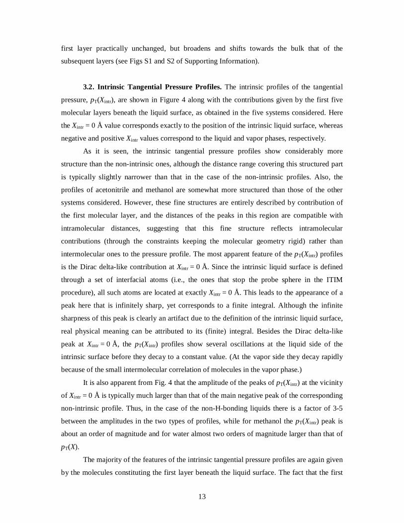
3.2. Intrinsic Tangential Pressure Profiles. The intrinsic profiles of the tangential

pressure, pT(Xintr), are shown in Figure 4 along with the contributions given by the first five

molecular layers beneath the liquid surface, as obtained in the five systems considered. Here

the Xintr = 0 Å value corresponds exactly to the position of the intrinsic liquid surface, whereas

negative and positive Xintr values correspond to the liquid and vapor phases, respectively.

As it is seen, the intrinsic tangential pressure profiles show considerably more

structure than the non-intrinsic ones, although the distance range covering this structured part

is typically slightly narrower than that in the case of the non-intrinsic profiles. Also, the

profiles of acetonitrile and methanol are somewhat more structured than those of the other

systems considered. However, these fine structures are entirely described by contribution of

the first molecular layer, and the distances of the peaks in this region are compatible with

intramolecular distances, suggesting that this fine structure reflects intramolecular

contributions (through the constraints keeping the molecular geometry rigid) rather than

intermolecular ones to the pressure profile. The most apparent feature of the pT(Xintr) profiles

is the Dirac delta-like contribution at Xintr = 0 Å. Since the intrinsic liquid surface is defined

through a set of interfacial atoms (i.e., the ones that stop the probe sphere in the ITIM

procedure), all such atoms are located at exactly Xintr = 0 Å. This leads to the appearance of a

peak here that is infinitely sharp, yet corresponds to a finite integral. Although the infinite

sharpness of this peak is clearly an artifact due to the definition of the intrinsic liquid surface,

real physical meaning can be attributed to its (finite) integral. Besides the Dirac delta-like

peak at Xintr = 0 Å, the pT(Xintr) profiles show several oscillations at the liquid side of the

intrinsic surface before they decay to a constant value. (At the vapor side they decay rapidly

because of the small intermolecular correlation of molecules in the vapor phase.)

It is also apparent from Fig. 4 that the amplitude of the peaks of pT(Xintr) at the vicinity

of Xintr = 0 Å is typically much larger than that of the main negative peak of the corresponding

non-intrinsic profile. Thus, in the case of the non-H-bonding liquids there is a factor of 3-5

between the amplitudes in the two types of profiles, while for methanol the pT(Xintr) peak is

about an order of magnitude and for water almost two orders of magnitude larger than that of

pT(X).

The majority of the features of the intrinsic tangential pressure profiles are again given

by the molecules constituting the first layer beneath the liquid surface. The fact that the first

14

layer molecules contribute to pT(Xintr) other than just at Xintr = 0 Å is due to the fact that the

layers have been defined in terms of molecules, whereas the tangential pressure is distributed

among the atoms in the system. In other words, atoms of the surface molecules that are

located right at the surface themselves (i.e., those that stop the probe sphere in the ITIM

procedure) give rise to the Dirac delta-like peak, while the other atoms belonging to the

surface molecules give rise to the contributions at non-zero Xintr values. It should also be

noted that the features of the pT(Xintr) profiles that correspond to the first molecular layer are

of little interest for our purpose, as they simply describe how the pressure is distributed within

the molecules.

While the contribution of the first molecular layer already largely describes the entire

pT(Xintr) profile in every case, the contribution of the second layer is still noticeable in every

case. Thus, in CCl4 and acetone the second layer contribution fully accounts for the negative

peak at about Xintr = -7 Å and the positive peak around Xintr = -3 Å, in acetonitrile it describes

the waves of pT(Xintr) between -10 and -5 Å, and contributes to the negative peak around -4 Å,

in methanol it gives rise to the small positive peaks at about -5 and -3 Å, and in water it

describes the features of pT(Xintr) between about -4 and -2 Å. On the other hand, the

contributions of the third to fifth layers to the intrinsic tangential pressure profiles, in a clear

contrast to those to the non-intrinsic profiles, are indeed featureless, flat curves.

Finally, it should be noted that the intrinsic tangential pressure profiles show several

details that are not seen in the non-intrinsic profiles. Thus, the intrinsic profiles exhibit

considerably more features in a considerably narrower distance range than the non-intrinsic

ones. Thus, in contrast with the rather complex structure of the intrinsic profiles, the non-

intrinsic ones exhibit one single negative peak, the amplitude of which is also much smaller

than those of the corresponding intrinsic profiles. All these changes reflect how the real,

molecular level structure of the liquid surface is washed out by neglecting the effect of the

capillary waves in a non-intrinsic analysis.

3.3. Contributions of the Individual Molecular Layers to the Surface Tension. The

net contribution of the subsequent molecular layers beneath the liquid surface to the value of

the tangential pressure can be calculated simply by integrating their individual contributions

to the tangential pressure profile. Here it is important to notice that it is not possible to

decompose the normal pressure component into layer contributions, and therefore, strictly

speaking, also the layer contribution to the full surface tension is not accessible, but only its

tangential contribution. However, since the normal pressure must be constant along the

15

interface normal axis, it is sensible to assume that each layer contributes roughly equally to it,

and through it also to the total value of the surface tension. Further, inside the bulk phases the

tangential and normal pressure components must be equal to each other and constant along

the interface normal axis. It is also clear from Figures 3 and 4 that this constant value is

several orders of magnitude smaller than the amplitude of the peaks of the tangential profile

(both in the intrinsic and non-intrinsic case). Therefore, apart from the first few molecular

layers, the difference of the normal and tangential pressure components (which, in turn, really

contributes to the surface tension, see eq. 1) must be zero, whereas in the first few layers the

(unknown) normal pressure component must be much smaller than the tangential one, and

hence can be neglected. In this sense, the tangential pressure contributions of the individual

molecular layers can be interpreted as being practically equal to their full surface tension

contributions. Thus, the term of the ’surface tension contribution’, when speaking about

individual molecular layers, is used and has to be interpreted in the above sense throughout

this paper.

The obtained contributions of the first four molecular layers to the surface tension (in

percentage) are shown in Figure 5. (The contribution of the fifth layer turned out to be

negligible in every case). As a check of consistency, we have done this calculation by

integrating both the intrinsic and non-intrinsic pressure profile contributions; the obtained

results agreed within 0.1% in every case. As is seen, the distribution of the surface tension

among the molecular layers is rather similar in the different liquids considered, in spite of the

fact that they correspond to markedly different intermolecular interactions. Thus, the vast

majority, i.e., at least 85% of the surface tension is concentrated in the first molecular layer;

the second layer still gives a noticeable, roughly 10% contribution to the surface tension,

while this contribution is already negligible beyond the second layer in every case. The only

exception in this respect is methanol, in which practically the entire surface tension comes

from the first molecular layer.

It is also apparent from Fig. 5 that several layers give a negative contribution to the

surface tension value. To understand the origin of this finding one has to consider that

although the origin of the surface tension is the loss of attractive interaction of molecules

being at the boundary of their phase, the surface tension itself describes the free energy cost of

molecules being at the surface. More specifically, in order to decrease their energy loss

surface molecules can increase their orientational order, both relative to the surface and to

each other, which eventually leads the decrease of their entropy. However, while this

orientational ordering might mostly or exclusively affect the surface layer itself, the

16

corresponding energy gain can also affect the neighboring layers, which can lead to a net free

energy decrease (i.e., negative surface tension contribution) in certain layers. This free energy

decrease is, however, not supposed to be large; in accordance with our finding that such

negative contribution to never exceeds 1.5%.

Although the general trends in the distribution of the surface tension clearly turn out to

be system independent, details of the whole picture still depend on the particular

intermolecular interactions acting in the different liquids. Thus, the roughly 10% contribution

of the second layer reflects the lack of attractive interaction of these molecules with several

second shell neighbors. In methanol, however, this contribution is completely missing. As it is

known, in methanol the surface molecules adopt a rather strong orientational order, preferring

the alignment in which the CH3 group sticks straight out to the vapor phase. This orientation

allows the surface methanol molecules to maintain all of their possible hydrogen bonds, and

therefore to fully preserve their hydrogen bonding structure,43,44 which leads to a much lower

surface tension value than what could be expected considering the strength of the

intermolecular interactions. Since in methanol H-bonding is the dominant interaction, but the

vicinity of the interface leaves the H-bonding structure of the molecules unchanged,

molecules in the second layer lack only a negligible fraction of their attractive interaction with

respect to the bulk phase ones. On the other hand, in water the surface molecules adopt

orientations such that they can form as many hydrogen bonds with each other as possible.5,43

As a price for that, hydrogen bonding between the first and second layers is, on average,

weaker than in the bulk liquid phase.

Finally, it should also be noted that the obtained contributions of the individual

molecular layers to the surface tension depend slightly also on the probe sphere radius used in

the analysis, although the global picture is insensitive to that. Thus, when using a probe

sphere of the radius of 1.2 Å instead of 2 Å for water, the contribution of the first and second

layer turns out to be 96.3% and 3.8%, respectively, while that of the subsequent layers is

practically zero. Similarly, when using the Rp value of 1.65 Å instead of 2 Å for methanol, the

contribution of the first three layers turns out to be 106.1%, -3.5% and -1.3%, respectively.

The fact that the decrease of the probe sphere radius leads to an increased contribution of the

first layer is consistent with the previous finding that it shifts the peaks of the subsequent

molecular layers contributions towards the bulk liquid phase (see Figs. S1 and S2 of

Supporting Information), and can be explained by the fact that smaller probe spheres can fall

deeper (with respect to larger ones) between the molecules, touching molecules located

farther from the liquid surface.5

17

4. Summary and Conclusions

In this paper we have demonstrated how intrinsic surface analysis methods can

provide a deep insight into the thermodynamics of fluid surfaces, by calculating the tangential

pressure profile across the liquid-vapor interface of five molecular liquids, characterized by

markedly different intermolecular interactions. Since the value of the surface tension can be

obtained by integrating the tangential pressure profile, this profile provides direct information

on how the surface tension is distributed along the interface normal axis.

Our results show a surprising insensitivity of this distribution of the surface tension to

the type of intermolecular interactions acting in the liquid phase. Thus, in every case, the vast

majority, i.e., at least 85% of the surface tension comes from the first molecular layer, while,

with the exception of methanol, the second layer contributes roughly 10% to the surface

tension, and the contributions of the subsequent molecular layers are negligible. In methanol,

on the other hand, the entire surface tension comes practically from the molecules constituting

the first layer. Correspondingly, when considering an external (i.e., non-intrinsic) coordinate

frame, the surface tension is distributed in a 1-2 nm broad interval along the surface normal,

which covers the distance range in which the first molecular layer is located. Considering an

intrinsic frame, i.e., calculating the profile relative to the capillary wave corrugated interface

itself, the distance range covering non-negligible surface tension contributions is even slightly

narrower, and the amplitudes of the peaks of the profile are considerably larger than in the

non-intrinsic case. The intrinsic analysis of the contribution of the subsequent molecular

layers to the profile also reveals that practically no surface tension contribution comes from

the third and subsequent molecular layers. By contrast, in a non-intrinsic treatment this

information is obscured by the effect of neglecting the capillary waves in the analysis.

Although the distribution of the surface tension along the surface normal axis turned

out to be largely independent from the interactions acting between the molecules in the

specific systems, several details of it still reflect the peculiarities of these intermolecular

interactions. Thus, in the case of water, characterized by small molecular size, particularly

strong interactions and, consequently, particularly close contact of the molecules, the featured

part of the surface tension profile is unusually narrow and the amplitudes of its peaks are

considerably larger than what could be expected simply from the value of the surface tension.

Also, due to the relatively weak interaction between the first two molecular layers beneath the

liquid surface, the contribution of the second layer to the surface tension is somewhat larger in

18

water than in the other liquids. By contrast, the strong surface orientation of the molecules at

the surface of methanol not only efficiently reduces the surface tension, but also eliminates

practically the contribution of the second layer.

Supporting Information. Contributions of the first five layers to the non-intrinsic

tangential pressure profile in water and methanol are provided, as obtained using probe

spheres of different radii. This information is available free of charge via the Internet at

http://pubs.acs.org.

Acknowledgements. This work has been supported by the Hungarian NKFIH

Foundation under Project No. NKFIH 119732, and by the Action Austria-Hungary

Foundation under project No. 93öu3.

References

(1) Chacón, E.; Tarazona, P. Intrinsic Profiles beyond the Capillary Wave Theory: A

Monte Carlo Study. Phys Rev. Letters 2003, 91, 166103-1-4.

(2) Mezei, M. A New Method for Mapping Macromolecular Topography. J. Mol.

Graphics Modell. 2003, 21, 463-472.

(3) Chowdhary, J.; Ladanyi, B. M. Water-Hydrocarbon Interfaces: Effect of Hydrocarbon

Branching on Interfacial Structure. J. Phys. Chem. B. 2006, 110, 15442-15453.

(4) Jorge, M.; Cordeiro, M. N. D. S. Intrinsic Structure and Dynamics of the

Water/Nitrobenzene Interface. J. Phys. Chem. C. 2007, 111, 17612-17626.

(5) Pártay, L. B.; Hantal, G.; Jedlovszky, P.; Vincze, Á.; Horvai, G. A New Method for

Determining the Interfacial Molecules and Characterizing the Surface Roughness in

Computer Simulations. Application to the Liquid–Vapor Interface of Water. J. Comp.

Chem. 2008, 29, 945-956.

(6) Wilard, A. P.; Chandler, D. Instantaneous Liquid Interfaces. J. Phys. Chem. B. 2010,

114, 1954-1958.

(7) Jorge, M.; Jedlovszky, P.; Cordeiro, M. N. D. S. A Critical Assessment of Methods for

the Intrinsic Analysis of Liquid Interfaces. 1. Surface Site Distributions. J. Phys.

Chem. C. 2010, 114, 11169-11179.

19

(8) Sega, M.; Kantorovich, S.; Jedlovszky, P; Jorge, M. The Generalized Identification of

Truly Interfacial Molecules (ITIM) Algorithm for Nonplanar Interfaces. J. Chem.

Phys. 2013, 138, 044110-1-10.

(9) Jorge, M.; Hantal, G.; Jedlovszky, P.; Cordeiro, M. N. D. S. A Critical Assessment of

Methods for the Intrinsic Analysis of Liquid Interfaces: 2. Density Profiles. J. Phys.

Chem. C. 2010, 114, 18656-18663.

(10) Sega, M.; Fábián, B.; Jedlovszky, P. Layer-by-Layer and Intrinsic Analysis of

Molecular and Thermodynamic Properties across Soft Interfaces. J. Chem. Phys. 2015,

143, 114709-1-8.

(11) Rowlinson, J. S.; Widom, B. Molecular Theory of Capillarity; Dover Publications:

Mineola, 2002, p. 11.

(12) Schofield, P.; Henderson, J. R. Statistical Mechanics of Inhomogeneous Fluids. Proc.

R. Soc. Lond. A 1982, 379, 231-246.

(13) Irving, J. H.; Kirkwood, J. G. The Statistical Mechanical Theory of Transport

Processes. IV. The Equations of Hydrodynamics. J. Chem. Phys. 1950, 18, 817-829.

(14) Harasima, A. Molecular Theory of Surface Tension. Adv. Chem. Phys. 1958, 1, 203-

237.

(15) Sonne, J.; Hansen, F. Y.; Peters, G. H. Methodological Problems in Pressure Profile

Calculations for Lipid Bilayers. J. Chem. Phys. 2005, 122, 124903-1-9.

(16) Ewald, P. Die Berechnung Optischer und Elektrostatischer Gitterpotentiale. Ann.

Phys. 1921, 369, 253–287.

(17) de Leeuw, S. W.; Perram, J. W.; Smith, E. R. Simulation of Electrostatic Systems in

Periodic Boundary Conditions. I. Lattice Sums and Dielectric Constants. Proc. R. Soc.

Lond. A 1980, 373, 27-56.

(18) Allen, M. P.; Tildesley, D. J. Computer Simulation of Liquids; Clarendon Press:

Oxford, 1987.

(19) Darden, T.; York, D.; Pedersen, L. Particle Mesh Ewald: An N·log(N) Method for

Ewald Sums in Large Systems. J. Chem. Phys. 1993, 98, 10089-10092.

(20) Essman, U.; Perera, L.; Berkowitz, M. L.; Darden, T.; Lee, H.; Pedersen, L. G. A

Smooth Particle Mesh Ewald Method. J. Chem. Phys. 1995, 103, 8577-8594.

(21) Sega, M.; Fábián, B.; Jedlovszky, P. Pressure Profile Calculation with Particle Mesh

Ewald Methods. J. Chem. Theory Comput. 2016, 12, 4509-4515.

20

(22) Pálinkás, G.; Hawlicka, E.; Heinzinger, K. A Molecular Dynamics Study of Liquid

Methanol with a Flexible Three-Site Model. J. Phys. Chem. 1987, 91, 4334-4341.

(23) Geiger, A.; Stillinger, F. H.; Rahman, A. Aspects of the Percolation Process for

Hydrogen-Bond Networks in Water. J. Chem. Phys. 1979, 70, 4185-4193.

(24) Stanley, H. E.; Teixeira, J. Interpretation of the Unusual Behavior of H2O and D2O at

Low Temperatures. Test of a Percolation Model. J. Chem. Phys. 1980, 73, 3404-3422.

(25) Duffy, E. M.; Severance, D. L.; Jorgensen, W. L. Solvent Effects on the Barrier to

Isomerization for a Tertiary Amide from Ab Initio and Monte Carlo Calculations. J.

Am. Chem. Soc. 1992, 114, 7535–7542.

(26) Stubbs, J. M.; Potoff, J. J.; Siepmann, J. I. Transferable Potentials for Phase

Equilibria. 6. United-Atom Description for Ethers, Glycols, Ketones, and Aldehydes.

J. Phys. Chem. B 2004, 108, 17596-17605.

(27) Böhm, H. J.; McDonald, I. R.; Madden, P. A. An Effective Pair Potential for Liquid

Acetonitrile. Mol. Phys. 1983, 49, 347-360.

(28) Walser, R.; Mark, A. E.; van Gunsteren, W. F.; Lauterbach , M.; Wipff, G. The Effect

of Force-Field Parameters on Properties of Liquids: Parametrization of a Simple

Three-Site Model for Methanol. J. Chem. Phys. 2000, 112, 10450-10459.

(29) Berendsen, H. J. C.; Grigera, J. R.; Straatsma, T. The Missing Term in Effective pair

Potentials. J. Phys. Chem. 1987, 91, 6269-6271.

(30) Berendsen, H. J. C.; Postma, J. P. M.; van Gunsteren, W. F.; Hermans, J. Interaction

Models for Water in Relation to Protein Hydration. In Intermolecular Forces;

Pullman, B., Ed.; Reidel: Dordrecht, 1981, p. 331-342.

(31) Jorgensen, W. L.; Chandrashekar, J.; Madura, J. D.; Impey, R.; Klein, M. L.

Comparison of Simple Potential Functions for Simulating Liquid Water. J. Chem.

Phys. 1983, 79, 926-935.

(32) Ryckaert, J. P.; Ciccotti, G.; Berendsen, H. J. C. Numerical Integration of the

Cartesian Equations of Motion of a System With Constraints; Molecular Dynamics of

n-Alkanes. J. Comp. Phys. 1977, 23, 327–341.

(33) Trokhymchuk, A.; Alejandre, J. Computer Simulations of Liquid/Vapor Interface in

Lennard-Jones Fluids: Some Questions and Answers. J. Chem. Phys. 1999, 111, 8510-

8523.

(34) in ’t Veld, P. J.; Ismail, A. E.; Grest, G. S. Application of Ewald Summations to Long-

Range Dispersion Forces. J. Chem. Phys. 2007, 127, 144711-1-8.

21

(35) Pronk, S.; Páll, S.; Schulz, R.; Larsson, P.; Bjelkmar, P.; Apostolov, R.; Shirts, M. R.;

Smith, J. C.; Kasson, P. M.; van der Spoel; D., et al. GROMACS 4.5: A High-

Throughput and Highly Parallel Open Source Molecular Simulation Toolkit.

Bioinformatics 2013, 29, 845–854.

(36) The code is freely available at https://github.com/Marcello-Sega/gromacs/tree/virial/.

(37) Nosé, S. A Molecular Dynamics Method for Simulations in the Canonical Ensemble.

Mol. Phys. 1984, 52, 255-268.

(38) Hoover, W. G. Canonical Dynamics: Equilibrium Phase-Space Distributions. Phys.

Rev. A 1985, 31, 1695-1697.

(39) Parrinello, M.; Rahman, A. Polymorphic Transitions in Single Crystals: A New

Molecular Dynamics Method. J. Appl. Phys. 1981, 52, 7182-7190.

(40) Pártay, L. B.; Horvai, G.; Jedlovszky, P. Temperature and Pressure Dependence of the

Properties of the Liquid-Liquid Interface. A Computer Simulation and Identification

of the Truly Interfacial Molecules Investigation of the Water-Benzene System. J.

Phys. Chem. C. 2010, 114, 21681-21693.

(41) Darvas, M.; Jorge, M.; Cordeiro, M. N. D. S.; Kantorovich, S. S.; Sega, M.;

Jedlovszky, P. Calculation of the Intrinsic Solvation Free Energy Profile of an Ionic

Penetrant Across a Liquid/Liquid Interface with Computer Simulations. J. Phys.

Chem. B 2013, 117, 16148-16156.

(42) Sega, M. The Role of a Small-Scale Cutoff in Determining Molecular Layers at Fluid

Interfaces. Phys. Chem. Chem. Phys. 2016, 18, 23354-23357.

(43) Pártay, L. B.; Jedlovszky, P.; Vincze, Á.; Horvai, G. Properties of Free Surface of

Water-Methanol Mixtures. Analysis of the Truly Interfacial Molecular Layer in

Computer Simulation. J. Phys. Chem. B. 2008, 112, 5428-5438.

(44) Idrissi, A.; Hantal, G.; Jedlovszky, P. Properties of the Liquid-Vapor Interface of

Acetone-Methanol Mixtures, as Seen from Computer Simulation and ITIM Surface

Analysis. Phys. Chem. Chem. Phys. 2015, 17, 8913-8926.

22

Tables

TABLE 1. Interaction Parameters of the Molecular Models Used.

molecule interaction site /Å /kJ mol-1 q/e

C 3.800 0.2093 0.248 CCl4a

Cl 3.470 1.1137 -0.062

CH3 3.790 0.8144 0.000

acetoneb C 3.820 0.3324 0.424

O 3.050 0.6565 -0.424

H 2.200 0.0835 0.201

C(H3) 3.000 0.4177 -0.577 acetonitrilec

C(≡N) 3.400 0.4177 0.488

N 3.300 0.4177 -0.514

CH3 3.601 1.0168 0.266

methanold O 3.176 0.5519 -0.674

H - - 0.408

O 3.166 0.6502 -0.820 watere

H - - 0.410 aOPLS model, Ref. 25. bTraPPE model, Ref. 26. cRef. 27. dRef. 28. eSPC/E model, Ref. 29.

23

Figure legend

Figure 1. Schematic structure of the five molecules considered in this study. C, Cl, O, N, and

H atoms are marked by grey, light blue, red, dark blue, and white colors, respectively. H

atoms are only shown when the molecular model used treats them explicitly.

Figure 2. Equilibrium snapshot of the surface portion of the five interfacial systems

simulated. Molecules belonging to the first, second, third, fourth and fifth molecular layers are

marked by blue, red, green, magenta, and brown colors, while those belonging to the bulk

liquid phase (i.e. located beyond the fifth layer) and vapor phases by gray and yellow colors,

respectively.

Figure 3. Non-intrinsic (i.e., relative to the basic simulation box) profile of the tangential

pressure (black solid lines) at the liquid-vapor interface of CCl4 (top panel), acetone (second

panel), acetonitrile (third panel), methanol (fourth panel), and water (bottom panel), as

obtained from our computer simulations. The contributions given by the first (red squares),

second (green circles), third (blue up triangles), fourth (light blue down triangles) and fifth

(magenta open diamonds) molecular layers beneath the liquid surface to these profiles are also

indicated. The insets show the structured part of the profiles on a magnified scale.

Figure 4. Intrinsic (i.e., relative to the capillary wave corrugated liquid surface) profile of the

tangential pressure (black solid lines) at the liquid-vapor interface of CCl4 (top panel), acetone

(second panel), acetonitrile (third panel), methanol (fourth panel), and water (bottom panel),

as obtained from our computer simulations. The contributions given by the first (red squares),

second (green circles), third (blue up triangles), fourth (light blue down triangles) and fifth

(magenta open diamonds) molecular layers beneath the liquid surface to these profiles are also

indicated.

Figure 5. Net contribution of the first four molecular layers beneath the liquid surface to the

value of the surface tension, as obtained at the liquid-vapor interface of CCl4 (top panel),

acetone (second panel), acetonitrile (third panel), methanol (fourth panel), and water (bottom

panel). The corresponding values are also shown numerically.

24

Figure 1.

Sega et al.

CCl4 acetone acetonitrile methanol water

25

Figure 2.

Sega et al.

acetonitrile

acetone

methanol

water

CCl4

26

Figure 3.

Sega et al.

0 30 60 90 120 150-2000-1500-1000-500

0500

-300-200-100

0100

-300-200-100

0100

-250-200-150-100-50

050

-200-150-100-50

050

10 15 20 25 30-2000-1500

-1000-500

0

500

30 40 50 60

-300

-200

-100

0

100

40 50 60 70 80-300

-200

-100

0

80 100 120-200

-150

-100

-500

50100 120 140

-150

-100

-50

0

p T(X)/b

ar

Water

X/Å

Methanol

Acetonitrile

Acetone

CCl4

pT(X

)/bar

X/Å

pT(X

)/bar

X/Å

X/Å pT(X

)/bar

pT(X

)/bar

X/Å

pT(X

)/bar

X/Å

27

Figure 4.

Sega et al.

-15 -10 -5 0 5-120000

-90000

-60000

-30000

0-4500-3000-1500

015003000-250

0250500750

-1000-750-500-250

0250

-750

-500

-250

0

250

p T(Xin

tr)/bar

Water

Xintr/Å

Methanol

Acetonitrile

Acetone

CCl4

28

Figure 5.

Sega et al.

0

25

50

75

1000

25

50

75

1000

25

50

75

1000

25

50

75

100

1 2 3 40

25

50

75

100

0.1%2.6%85.4% 11.8%

water

surfa

ce te

nsio

n co

ntrib

utio

n (%

)

layer

-0.7%-0.8%102.4% -0.6%

methanol

0.1%88.2% 10.9%

acetonitrile

-1.4%-0.8%94.2% 9.5%

acetone

-0.7%-0.9%

1.1%

10.3%92.0%

CCl4

29

Table of Contents Graphics:

0 30 60 90

2

4

5

3

1

%

laye

r