How Large are the Gains from Economic Integration? …ies/IESWorkshopS2011/DonaldsonPaper.pdfHow Large are the Gains from Economic Integration? Theory and Evidence from U.S ... ment

How Large are the Gains from Economic Integration?

Theory and Evidence from U.S. Agriculture, 1840-2002

Arnaud Costinot

MIT and NBER

Dave Donaldson

MIT, NBER and CIFAR

PRELIMINARY AND INCOMPLETE

PLEASE DO NOT CIRCULATE

June 20, 2011

Abstract

In this paper we develop a new approach to measuring the gains from economic

integration based on a Roy-like assignment model in which heterogeneous factors of

production are allocated to multiple sectors in multiple local markets. We imple-

ment this approach using data on crop markets in 1,250 U.S. counties from 1840 to

2002. Central to our empirical analysis is the use of a novel agronomic data source on

predicted output by crop for small spatial units. Crucially, this dataset contains infor-

mation about the productivity of all units for all crops, not just those that are actually

being grown. Using this new approach we estimate: (i) the spatial distribution of price

wedges across U.S. counties from 1840 to 2002; (ii) the gains associated with changes

in the level of these wedges over time; and (iii) the further gains that could obtain if

all wedges were removed and gains from market integration were fully realized.

1 Introduction

How large are the gains from economic integration? Since researchers never observe markets

that are both closed and open at the same time, the fundamental challenge in answering

this question lies in predicting how local markets, either countries or regions, would behave

under counterfactual scenarios in which they suddenly become more or less integrated with

the rest of the world.

One prominent response to this challenge, the “reduced form” approach, argues that

knowledge about such counterfactual scenarios can be obtained by comparing countries that

are more open to countries that are more closed (or analogously, by comparing a country

to itself before and after its level of trade openness changes).1 Frankel and Romer (1999)

is a well-known example. The implicit assumption about counterfactual scenarios embodied

in the reduced form approach is that currently open economies would behave, were they

to be less open, in exactly the same manner as countries that are currently less open are

currently behaving. An unsettled area of debate in this literature concerns the credibility

of this counterfactual assumption. Another weakness of this approach is that it does not

estimate policy invariant parameters of economic models, thereby limiting its relevance for

policy and welfare analysis.

Another prominent approach, the “structural” approach, aims to estimate or calibrate

fully specified models of how countries behave under any trading regime. Eaton and Kortum

(2002) is the most influential application of this approach in the international trade literature.

A core ingredient of such models is that there exists a set of technologies that a country would

have no choice but to use if trade was restricted, but which the country can choose not to

use when it is able to trade. Estimates of the gains from economic integration, however

defined, thereby require the researcher to compare factual technologies that are currently

being used to inferior, counterfactual technologies that are deliberately not being used and

are therefore unobservable to the researcher. This comparison is typically made through the

use of functional form assumptions that allow an extrapolation from observed technologies

to unobserved ones.

The goal of this paper is to develop a new structural approach with less need for ex-

trapolation by functional form assumptions in order to obtain knowledge of counterfactual

scenarios. Our basic idea is to focus on agriculture, a sector of the economy in which sci-

entific knowledge of how essential inputs such as water, soil and climatic conditions map

into outputs is uniquely well understood. As a consequence of this knowledge, agronomists

are able to predict– typically with great success– how productive a given parcel of land (a

‘field’) would be were it to be used to grow any one of a set of crops. Our approach combines

1We use the terms “reduced form”and “structural”in the same sense as, for example, Chetty (2009).

1

these agronomic predictions about factual and counterfactual technologies with a Roy-like

assignment model in which heterogeneous fields are allocated to multiple crops in multiple

local markets.

We implement our approach in the context of U.S. agricultural markets from 1840 to

2002. Our dataset consists of 1,250 U.S. counties which we treat as separate local markets

that may be segmented by barriers to trade– analogous to ‘countries’in a standard trade

model. Each county is endowed with many ‘fields’of arable land.2 At each of these fields,

a team of agronomists, as part of the Food and Agriculture Organization’s (FAO) Global

Agro-Ecological Zones (GAEZ) project, have used high-resolution data on soil, topography,

elevation and climatic conditions, fed into state-of-the-art models that embody the biology,

chemistry and physics of plant growth, to predict the quantity of yield that each field could

obtain if it were to grow each of 25 different crops. In our Roy-like assignment model, these

data are suffi cient to construct the production possibility frontier associated with each U.S.

county, which is the essential ingredient required to perform any counterfactual analysis.

Counterfactual analysis in our paper formally proceeds in two steps. First we combine the

productivity data from the GAEZ project with data from the decadal Agricultural Census

on the total amount of output of each crop in each county. Under perfect competition, we

demonstrate how this information can be used to infer local crop prices in each county and

time period as the solution of a simple linear programming problem. Second, armed with

these estimates of local crop prices, we compute the spatial distribution of price ‘wedges’

across U.S. counties from 1840 to 2002 and ask: “For any pair of periods, t and t′, how

much higher (or lower) would the total value of agricultural output across U.S. counties in

period t have been if wedges were those of period t′ rather than period t?”The answer to

this counterfactual question will be our measure of the gains (or losses) from changes in the

degree of economic integration in U.S. agricultural markets over time.

The rest of this paper is organized as follows. Section 3 introduces our theoretical frame-

work, describes how to measure local prices, and in turn, how to measure the gains from

economic integration. Section 4 describes our data. Section 5 presents our main empirical

results. Section 6 offers two extensions. Section 7 concludes. All formal proofs can be found

in the appendix.

2‘Fields’in our dataset are fairly large spatial units: the median U.S. county contains 26 fields.

2

2 Theoretical Framework

2.1 Endowments, Technology, and Market Structure

Our theoretical framework is a Roy-like assignment model, as in Costinot (2009). We consider

an economy with multiple local markets indexed by i ∈ I ≡{1, ..., I}. In our empiricalanalysis, a local market will be a US county. In each market, the only factors of production

are different types of land or fields indexed by f ∈ F ≡ {1, ..., F}. Li (f) ≥ 0 denotes the

number of acres covered by field f in market i. Fields can be used to produce multiple crops

indexed by c ∈ C ≡{1, ..., C}. Fields are perfect substitutes in the production of each crop,but vary in their productivity per acre, Aci (f) > 0. Total output Qci of crop c in market i is

given by

Qci =∑

f∈F Aci (f)Lci (f) ,

where Lci (f) ≥ 0 denotes the number of acres of field f allocated to crop c in market i. Note

that Aci (f) may vary both with f and c. Thus although fields are perfect substitutes in the

production of each crop, some fields may have a comparative as well as absolute advantage

in producing particular crops.

All crops are produced by a large number of price-taking farms in all local markets. The

profits of a representative farm producing crop c in market i are given by

Πci = pci

∑f∈F A

ci (f)Lci (f)− ri (f)Lci (f) ,

where pci and ri (f) denote the price of crop c and rental rate per acre of field f in market i,

respectively. Profit maximization by farms requires

pciAci (f)− ri (f) ≤ 0, for all c ∈ C, f ∈ F , (1)

pciAci (f)− ri (f) = 0, if Lci (f) > 0 (2)

Local factor markets are segmented. Thus factor market clearing in market i requires

∑c∈C L

ci (f) ≤ Li (f) , for all f ∈ F . (3)

We leave good market clearing conditions unspecified, thereby treating each local market as

a small open economy. In the rest of this paper we denote by pi ≡ (pci)c∈C the vector of crop

prices, ri ≡ [ri (f)]f∈F the vector of field prices, and Li ≡ [Lci (f)]c∈C,f∈F the allocation of

fields to crops in market i.

3

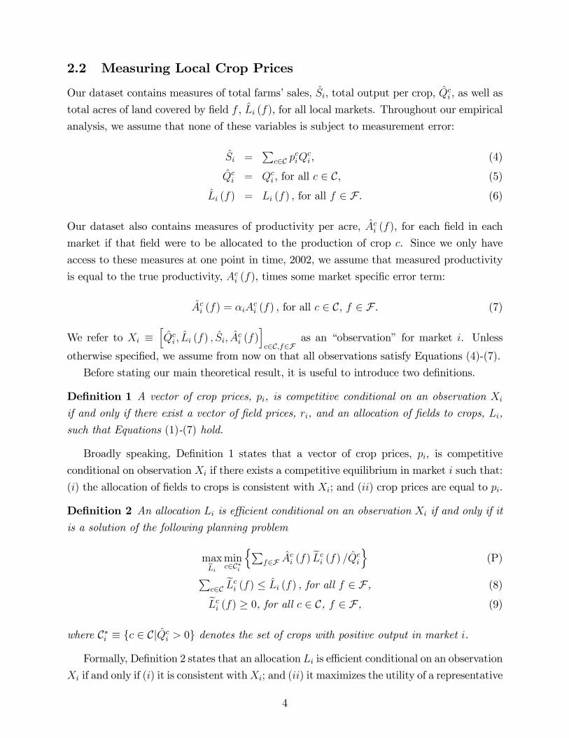
2.2 Measuring Local Crop Prices

Our dataset contains measures of total farms’sales, Si, total output per crop, Qci , as well as

total acres of land covered by field f , Li (f), for all local markets. Throughout our empirical

analysis, we assume that none of these variables is subject to measurement error:

Si =∑

c∈C pciQ

ci , (4)

Qci = Qci , for all c ∈ C, (5)

Li (f) = Li (f) , for all f ∈ F . (6)

Our dataset also contains measures of productivity per acre, Aci (f), for each field in each

market if that field were to be allocated to the production of crop c. Since we only have

access to these measures at one point in time, 2002, we assume that measured productivity

is equal to the true productivity, Aci (f), times some market specific error term:

Aci (f) = αiAci (f) , for all c ∈ C, f ∈ F . (7)

We refer to Xi ≡[Qci , Li (f) , Si, A

ci (f)

]c∈C,f∈F

as an “observation” for market i. Unless

otherwise specified, we assume from now on that all observations satisfy Equations (4)-(7).

Before stating our main theoretical result, it is useful to introduce two definitions.

Definition 1 A vector of crop prices, pi, is competitive conditional on an observation Xi

if and only if there exist a vector of field prices, ri, and an allocation of fields to crops, Li,

such that Equations (1)-(7) hold.

Broadly speaking, Definition 1 states that a vector of crop prices, pi, is competitive

conditional on observation Xi if there exists a competitive equilibrium in market i such that:

(i) the allocation of fields to crops is consistent with Xi; and (ii) crop prices are equal to pi.

Definition 2 An allocation Li is effi cient conditional on an observation Xi if and only if it

is a solution of the following planning problem

maxLi

minc∈C∗i

{∑f∈F A

ci (f) Lci (f) /Qci

}(P)∑

c∈C Lci (f) ≤ Li (f) , for all f ∈ F , (8)

Lci (f) ≥ 0, for all c ∈ C, f ∈ F , (9)

where C∗i ≡ {c ∈ C|Qci > 0} denotes the set of crops with positive output in market i.

Formally, Definition 2 states that an allocation Li is effi cient conditional on an observation

Xi if and only if (i) it is consistent withXi; and (ii) it maximizes the utility of a representative

4

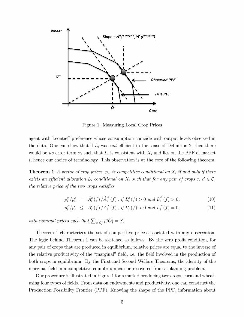
Figure 1: Measuring Local Crop Prices

agent with Leontieff preference whose consumption coincide with output levels observed in

the data. One can show that if Li was not effi cient in the sense of Definition 2, then there

would be no error term αi such that Li is consistent with Xi and lies on the PPF of market

i, hence our choice of terminology. This observation is at the core of the following theorem.

Theorem 1 A vector of crop prices, pi, is competitive conditional on Xi if and only if there

exists an effi cient allocation Li conditional on Xi such that for any pair of crops c, c′ ∈ C,the relative price of the two crops satisfies

pc′

i /pci = Aci (f) /Ac

′

i (f) , if Lci (f) > 0 and Lc′

i (f) > 0, (10)

pc′

i /pci ≤ Aci (f) /Ac

′


i (f) = 0, (11)

with nominal prices such that∑

c∈C∗ipciQ

ci = Si.

Theorem 1 characterizes the set of competitive prices associated with any observation.

The logic behind Theorem 1 can be sketched as follows. By the zero profit condition, for

any pair of crops that are produced in equilibrium, relative prices are equal to the inverse of

the relative productivity of the “marginal”field, i.e. the field involved in the production of

both crops in equilibrium. By the First and Second Welfare Theorems, the identity of the

marginal field in a competitive equilibrium can be recovered from a planning problem.

Our procedure is illustrated in Figure 1 for a market producing two crops, corn and wheat,

using four types of fields. From data on endowments and productivity, one can construct the

Production Possibility Frontier (PPF). Knowing the shape of the PPF, information about

5

relative output levels of the two crops can then be used to infer the slope of the PPF at the

observed vector of output, and in turn, the relative price of the two crops produced in this

market.

According to Theorem 1, one can infer the set of competitive crop prices by solving

a simple linear programming problem. Since our dataset includes 1,250 counties over 17

decades, this is very appealing from a computational standpoint. In spite of the high-

dimensionality of the problem we are interested in– the median U.S. county in our dataset

features 25 crops and 26 fields– it is therefore possible to characterize the set of competitive

crop prices in each county in a very limited amount of time using standard software packages.

Finally, note that for any pair of goods produced in a given local market, the relative

price is generically unique. Non-uniqueness may only occur if the observed vector of out-

put is colinear with a vertex of the production possibility frontier associated with observed

productivity levels and endowments. Not surprisingly, this situation will never occur in our

empirical analysis.

2.3 Measuring the Gains from Economic Integration

Before measuring the gains from economic integration, one first needs to take a stand on

how to measure economic integration across markets. Intuitively, the extent of economic

integration should be related to differences in local crop prices. For one thing, we know

that if crop markets were perfectly integrated, then crop prices should be the same across

markets. To operationalize that idea, we introduce the following definition.

Definition 3 For any pair of crops c, c′ ∈ C in any period t, we define the extent of eco-nomic integration between market i and some reference market as the percentage difference

or “wedge,” τ cit ≡ pct/pcit − 1, between the price of crop c in the two markets.

Armed with Definition 3, one can then estimate the gains (or losses) from changes in the

degree of economic integration across markets between two periods t and t′ > t by answering

the following counterfactual question:

How much higher (or lower) would the total value of output across local markets

in period t have been if wedges were those of period t′ rather than period t?

Formally, let (Qcit)′ denote the counterfactual output level of crop c in market i in period

t if farms in this market were maximizing profits facing the counterfactual prices (pcit)′ =

pct/ (1 + τ cit′) rather than the true prices pcit = pct/ (1 + τ cit). Using this notation, there are

two ways to express the gains (or losses) from changes in the degree of economic integration

6

between two periods t and t′ > t:

∆Itt′ ≡

∑i∈I∑

c∈C pct (Qcit)

′∑i∈I∑

c∈C pctQ

cit

− 1, (12)

∆IItt′ ≡

∑i∈I∑

c∈C (pcit)′ (Qcit)

′∑i∈I∑

c∈C pcitQ

cit

− 1. (13)

By construction, ∆Itt′ and∆II

tt′ both measure how much larger (or smaller) GDP in agriculture

would have been in period t if wedges were those of period t′ rather than those of period

t. These two metric, however, differ in terms of the economic interpretation being given to

these wedges. These different interpretations are reflected in the vector of prices used to

evaluate the total value of output.

In Equation (12), we use the reference prices both in the original and the counterfactual

equilibrium. Thus the implicit assumption underlying ∆Itt′ is that differences in local crop

prices reflect “true” distortions. In order to maximize welfare– whatever the underlying

preferences of the U.S. representative agent may be– farmers should be maximizing profits

taking the reference prices pct as given, but because of various policy reasons, they do not.

This first welfare metric is close in spirit to the measurement of the impact of misallocations

on TFP in Hsieh and Klenow (2009).

In Equation (13), by contrast, we use local prices both in the original and the coun-

terfactual equilibrium. The implicit assumption underlying ∆IItt′ is that differences in local

crop prices reflect “true”technological considerations. Under this interpretation of wedges,

farmers face the “right”prices, but producer prices are lower in local markets than in the

reference market because of the cost of shipping crops. This second metric is closer in spirit

to the measurement of the impact of trade costs in quantitative trade models; see e.g. Eaton

and Kortum (2002) and Waugh (2010).

A few comments are in order. First, it should be clear that, independently of whether

we use ∆Itt′ or ∆II

tt′ , our strategy only allows us to identify wedges relative to some reference

prices. This implies that measurement error in reference prices may affect our estimates

of the gains from economic integration. We come back to this important issue in the next

sections. Second, our strategy only allows us to identify the production gains from economic

integration. Since we do not have consumption data, our analysis will remain silent about

any consumption gains from economic integration.

7

3 Data

Our analysis draws on two main sources of data: predicted productivity by field and crop

(from the GAEZ project), aggregate county outputs by crop (from the US Agricultural

Census), and data on reference prices. We describe these here in turn.ur analysis draws on

three main sources of data.

3.1 Productivity Data

The first and most novel data source that we make use provides measures of productiv-

ity, Aci (f),by crop c, county i, and field f . These measures comes from the Global Agro-

Ecological Zones (GAEZ) project run by the Food and Agriculture Organization (FAO).3

The GAEZ aims to provide a resource that farmers and government agencies can use to make

decisions about the optimal crop choice in a given location that draw on the best available

agronomic knowledge of how crops grow under different conditions.

The core ingredient of the GAEZ predictions is a set of inputs that are known with

extremely high spatial resolution. This resolution governs the resolution of the final GAEZ

database and, equally, that of our analysis– what we call a ‘field’ (of which there are 26

in the median U.S. county) is the spatial resolution of GAEZ’s most spatially coarse input

variable. The inputs to the GAEZ database are data on an eight-dimensional vector of soil

types and conditions, the elevation, the average land gradient, and climatic variables (based

on rainfall, temperature, humidity, sun exposure), in each ‘field’. These inputs are then

fed into an agronomic model– one for each crop– that predicts how these inputs affect the

‘microfoundations’of the plant growth process and thereby map into crop yields. Naturally,

decisions by farmers about how to grow their crops and what complementary inputs (such

as irrigation) to use affect crop yields in addition to those inputs (such as sun exposure and

soil types) over which farmers have very little control. For this reason the GAEZ project

constructs different sets of productivity predictions for different scenarios of farmer inputs.

In our baseline results we use the GAEZ predictions that correspond to the ‘most active’

farmer decisions, and those that involve the highest level of irrigation. We also explore the

robustness of our results to alternative GAEZ modeling scenarios in Section 5.

Finally we wish to emphasize that while the GAEZ has devoted a great deal of attention

to testing their predictions on knowledge of actual growing conditions (e.g. under controlled

experiments at agricultural research stations) the GAEZ does not form its predictions by

estimating any sort of statistical relationship between observed inputs around the world and

3This database has been used by Nunn and Qian (2011) to obtain predictions about the potential pro-ductivity of European regions in producing potatoes, in order to estimate the effect of the discovery of thepotato on population growth in Europe.

8

observed outputs around the world.

3.2 Output Data

The second set of data that we draw on contains records of actual output, Qci , in each US

county from 1840-2002.4 These measures come from the decadal Census of Agriculture

that began in 1840. Although the total output of each crop in each decade in each county is

known, such measures are not available for spatial units smaller than the county (such as the

‘field’). Another source of contained in the Census of Agriculture is the area of land devoted

to each crop in each county and decade. Although this information was not necessary in the

methodology outlined above, it can be usefully applied to weaken the assumption that Aci (f)

can only be mismeasured by a Hicks-neutral term (in each time period), as we demonstrate

in Section 5.2. The weaker assumption is that Aci (f) can be mismeasured by a factor that

can be specific to each crop, county and time period (but this measurement error needs to

be constant across fields within a county, crop and time period).

3.3 Price Data

A final source of data that we will make use of is actual data on observed wholesale and

retail prices from as many cities, for as many crops, and in as many years as possible. We

will use these actual price observations to check that our inferred relative producer prices

agree with actual relative price data, at least in the vicinity of the few cities from which

actual price data are available.

For now, we will only work with the New York State price, which will take as a proxy

for the ‘world price’, which itself is our choice of the reference price at which to evaluate

counterfactual production scenarios. The earliest such data available are for 1860 (Craig,

1998). These data are only available for 9 of our crops, but these are the most important

crops in our dataset. In our empirical analysis, all other crops will be set to zero.

4 Empirical Results

This section presents very preliminary empirical results, based– for now– only on output

data from 1840 and 2002.4We use the 1,250 counties that reported agricultural output data in 1840, and only the corresponding

states in 2002 (which comprise, in essence, the Eastern half of the United States.)

9

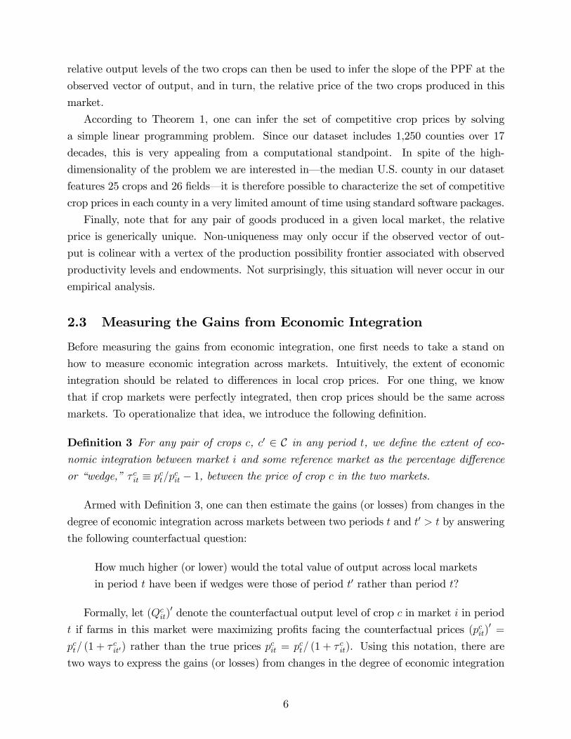
Dependent variable:

maize wheat

maize barley

maize cotton

(1) (2) (3)

1840 sample:distance between i and j 0.84 0.80 0.57

(0.0071)** (0.013)** (0.0056)**Observations 583,070 7,742 42,337

2000 sample:distance between i and j 0.16 0.25 0.00012

(0.029)** (0.089)** 0.00007Observations 567 139 3

Notes: Standard errors in parentheses. ** indicates statistically significant at 1% level.

gap in relative prices betweencounties i and j

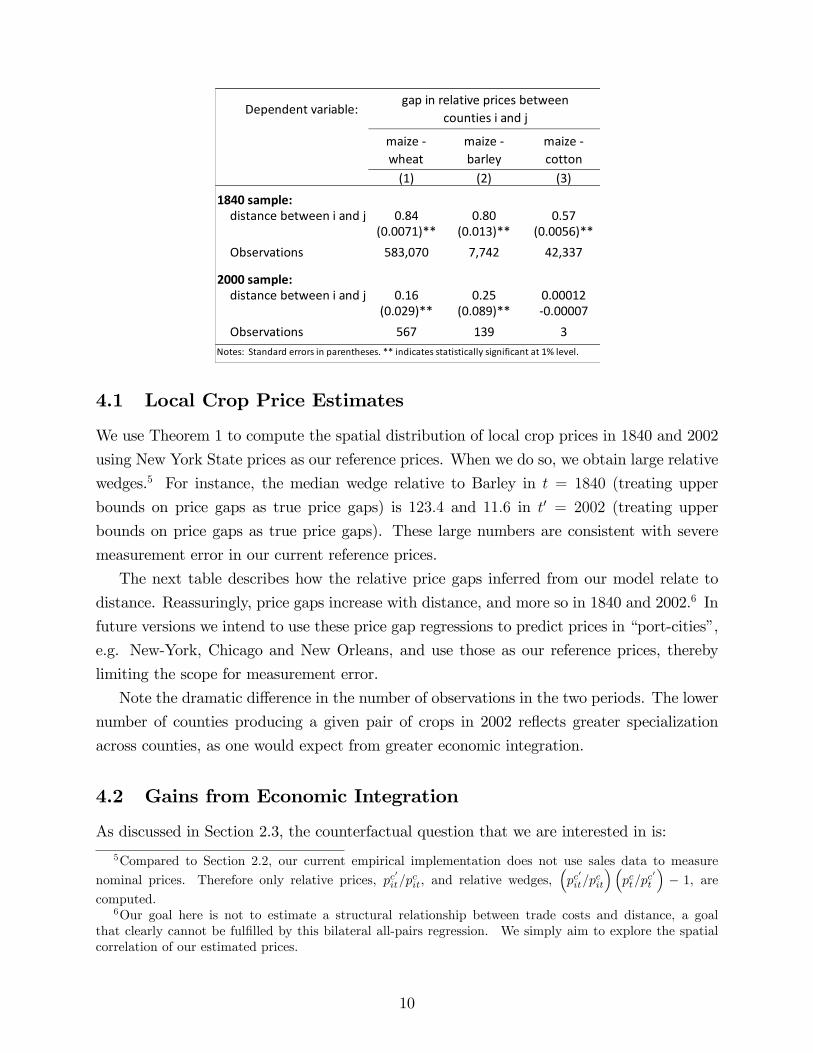
4.1 Local Crop Price Estimates

We use Theorem 1 to compute the spatial distribution of local crop prices in 1840 and 2002

using New York State prices as our reference prices. When we do so, we obtain large relative

wedges.5 For instance, the median wedge relative to Barley in t = 1840 (treating upper

bounds on price gaps as true price gaps) is 123.4 and 11.6 in t′ = 2002 (treating upper

bounds on price gaps as true price gaps). These large numbers are consistent with severe

measurement error in our current reference prices.

The next table describes how the relative price gaps inferred from our model relate to

distance. Reassuringly, price gaps increase with distance, and more so in 1840 and 2002.6 In

future versions we intend to use these price gap regressions to predict prices in “port-cities”,

e.g. New-York, Chicago and New Orleans, and use those as our reference prices, thereby

limiting the scope for measurement error.

Note the dramatic difference in the number of observations in the two periods. The lower

number of counties producing a given pair of crops in 2002 reflects greater specialization

across counties, as one would expect from greater economic integration.

4.2 Gains from Economic Integration

As discussed in Section 2.3, the counterfactual question that we are interested in is:

5Compared to Section 2.2, our current empirical implementation does not use sales data to measure

nominal prices. Therefore only relative prices, pc′

it/pcit, and relative wedges,

(pc

′

it/pcit

)(pct/p

c′

t

)− 1, are

computed.6Our goal here is not to estimate a structural relationship between trade costs and distance, a goal

that clearly cannot be fulfilled by this bilateral all-pairs regression. We simply aim to explore the spatialcorrelation of our estimated prices.

10

How much higher (or lower) would the total value of output across local markets

in period t have been if wedges were those of period t′ rather than period t?

Like in the previous section, we focus on two years t = 1840 and t′ = 2002. So far

we have only computed ∆Itt′ ≡

∑i∈I∑

c∈C pct (Qcit)

′ /∑

i∈I∑

c∈C pctQ

c′it − 1. Because we can’t

track counties from 1840 to 2002 (for now), we use average t′ = 2002 wedges here. We find

that output would have been worth 48% more (if upper bounds on price gaps are taken as

true values of price gaps) and 34% more, if upper bounds on price gaps are instead replaced

with zeroes. The total value of output would be 51% higher if there no wedges at all, i.e.

under perfectly free trade).

5 Extensions

We now present two theoretical extensions that are feasible, and probably important, but

have not been implemented empirically yet.

5.1 Non-Agricultural Land Use

The first of our two extensions allows for non-agricultural land uses, e.g. forests, services,

or manufacturing. For expositional purposes, we simply refer to such activities in short as

“manufacturing.”Crop production is as described in Section 2.1. But unlike in our baseline

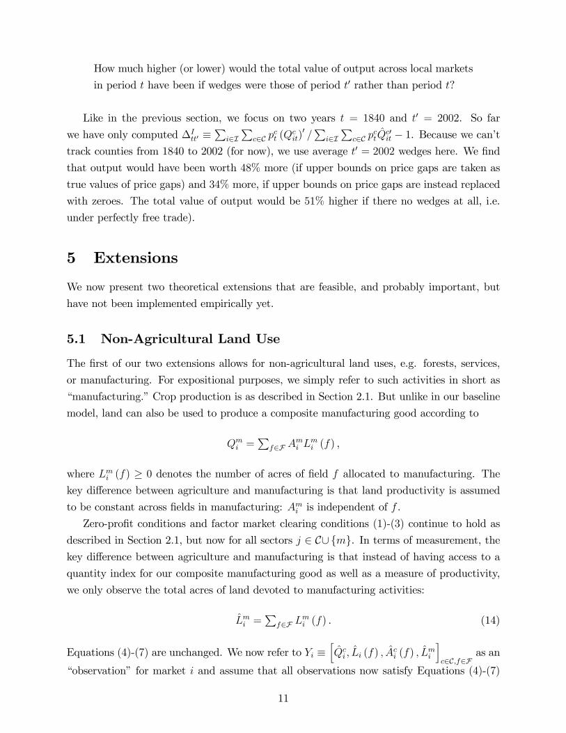
model, land can also be used to produce a composite manufacturing good according to

Qmi =∑

f∈F Ami L

mi (f) ,

where Lmi (f) ≥ 0 denotes the number of acres of field f allocated to manufacturing. The

key difference between agriculture and manufacturing is that land productivity is assumed

to be constant across fields in manufacturing: Ami is independent of f .

Zero-profit conditions and factor market clearing conditions (1)-(3) continue to hold as

described in Section 2.1, but now for all sectors j ∈ C∪{m}. In terms of measurement, thekey difference between agriculture and manufacturing is that instead of having access to a

quantity index for our composite manufacturing good as well as a measure of productivity,

we only observe the total acres of land devoted to manufacturing activities:

Lmi =∑

f∈F Lmi (f) . (14)

Equations (4)-(7) are unchanged. We now refer to Yi ≡[Qci , Li (f) , Aci (f) , Lmi

]c∈C,f∈F

as an

“observation” for market i and assume that all observations now satisfy Equations (4)-(7)

11

and (14). In this environment our definition of competitive prices and effi cient allocations

can be generalized as follows.

Definition 1(M) A vector of crop prices, pi, is competitive conditional on an observationYi if and only if there exist a vector of field prices, ri, and an allocation of fields to crops,

Li, such that Equations (1)-(7) and (14) hold.

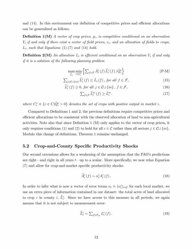
Definition 2(M) An allocation Li is effi cient conditional on an observation Yi if and onlyif it is a solution of the following planning problem

maxLi

minc∈C∗i

{∑f∈F A

ci (f) Lci (f) /Qci

}(P-M)∑

j∈C∪{m} Lji (f) ≤ Li (f) , for all f ∈ F , (15)

Lji (f) ≥ 0, for all j ∈ C∪{m} , f ∈ F , (16)∑f∈F L

mi (f) ≥ Lmi . (17)


Compared to Definitions 1 and 2, the previous definitions require competitive prices and

effi cient allocations to be consistent with the observed allocation of land to non-agricultural

activities. Note also that since Definition 1 (M) only applies to the vector of crop prices, it

only requires conditions (1) and (2) to hold for all c ∈ C rather than all sectors j ∈ C∪{m}.Modulo this change of definitions, Theorem 1 remains unchanged.

5.2 Crop-and-County Specific Productivity Shocks

Our second extensions allows for a weakening of the assumption that the FAO’s predictions

are right– and right in all years t– up to a scalar. More specifically, we now relax Equation

(7) and allow for crop-and-market specific productivity shocks:

Aci (f) = αciAci (f) . (18)

In order to infer what is now a vector of error terms αi ≡ (αci)c∈C for each local market, we

use an extra piece of information contained in our dataset: the total acres of land allocated

to crop c in county i, Lci . Since we have access to this measure in all periods, we again

assume that it is not subject to measurement error:

Lci =∑

f∈Fm Lci (f) . (19)

12

We now refer to Zi ≡[Qci , Li (f) , Si, A

ci (f) , Lci

]c∈C,f∈F

as an “observation”for market i and

assume that all observations now satisfy equations (4)-(6) and (18)-(19). In this environment,

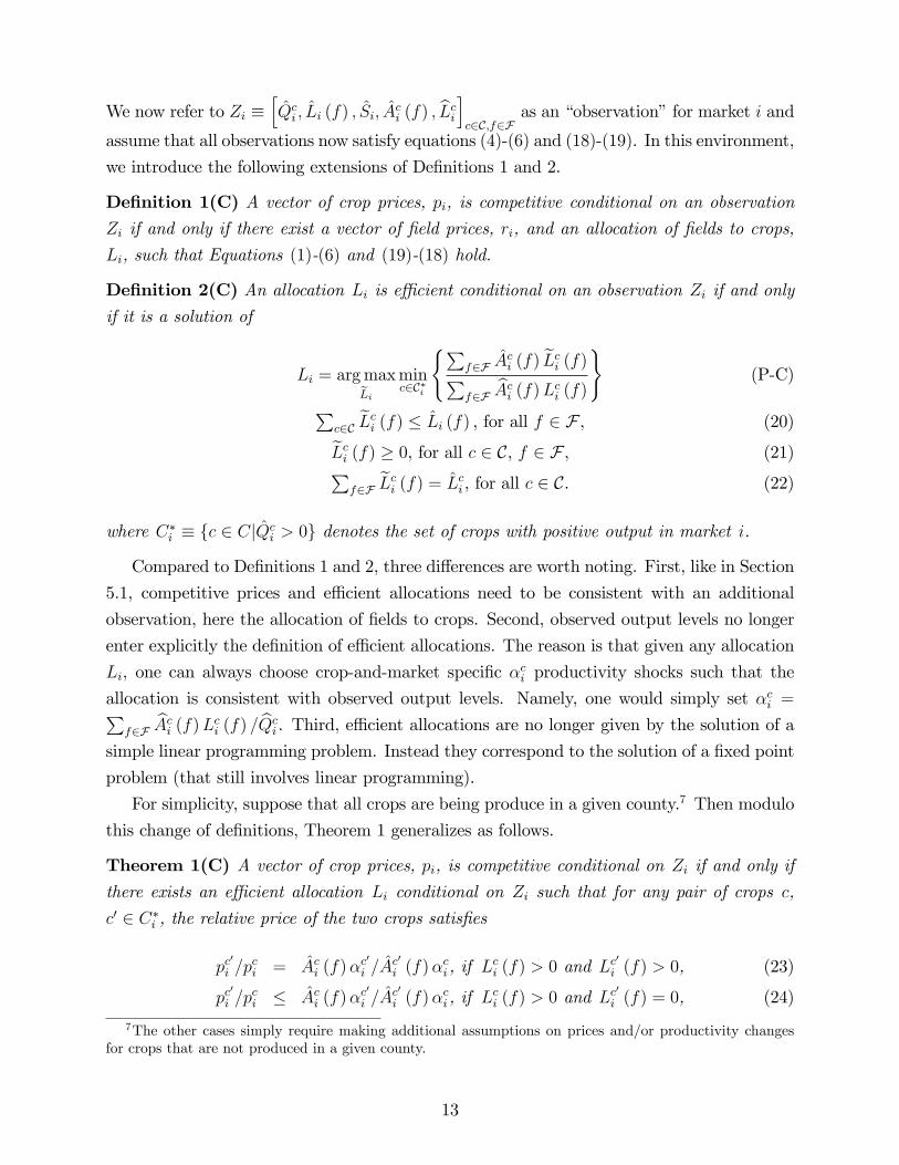
we introduce the following extensions of Definitions 1 and 2.

Definition 1(C) A vector of crop prices, pi, is competitive conditional on an observation

Zi if and only if there exist a vector of field prices, ri, and an allocation of fields to crops,

Li, such that Equations (1)-(6) and (19)-(18) hold.

Definition 2(C) An allocation Li is effi cient conditional on an observation Zi if and onlyif it is a solution of

Li = arg maxLi

minc∈C∗i

{∑f∈F A

ci (f) Lci (f)∑

f∈F Aci (f)Lci (f)

}(P-C)

∑c∈C L

ci (f) ≤ Li (f) , for all f ∈ F , (20)

Lci (f) ≥ 0, for all c ∈ C, f ∈ F , (21)∑f∈F L

ci (f) = Lci , for all c ∈ C. (22)


Compared to Definitions 1 and 2, three differences are worth noting. First, like in Section

5.1, competitive prices and effi cient allocations need to be consistent with an additional

observation, here the allocation of fields to crops. Second, observed output levels no longer

enter explicitly the definition of effi cient allocations. The reason is that given any allocation

Li, one can always choose crop-and-market specific αci productivity shocks such that the

allocation is consistent with observed output levels. Namely, one would simply set αci =∑f∈F A

ci (f)Lci (f) /Qci . Third, effi cient allocations are no longer given by the solution of a

simple linear programming problem. Instead they correspond to the solution of a fixed point

problem (that still involves linear programming).

For simplicity, suppose that all crops are being produce in a given county.7 Then modulo

this change of definitions, Theorem 1 generalizes as follows.

Theorem 1(C) A vector of crop prices, pi, is competitive conditional on Zi if and only if

there exists an effi cient allocation Li conditional on Zi such that for any pair of crops c,

c′ ∈ C∗i , the relative price of the two crops satisfies

pc′

i /pci = Aci (f)αc

′

i /Ac′

i (f)αci , if Lci (f) > 0 and Lc

′

i (f) > 0, (23)

pc′

i /pci ≤ Aci (f)αc

′

i /Ac′


′

i (f) = 0, (24)

7The other cases simply require making additional assumptions on prices and/or productivity changesfor crops that are not produced in a given county.

13

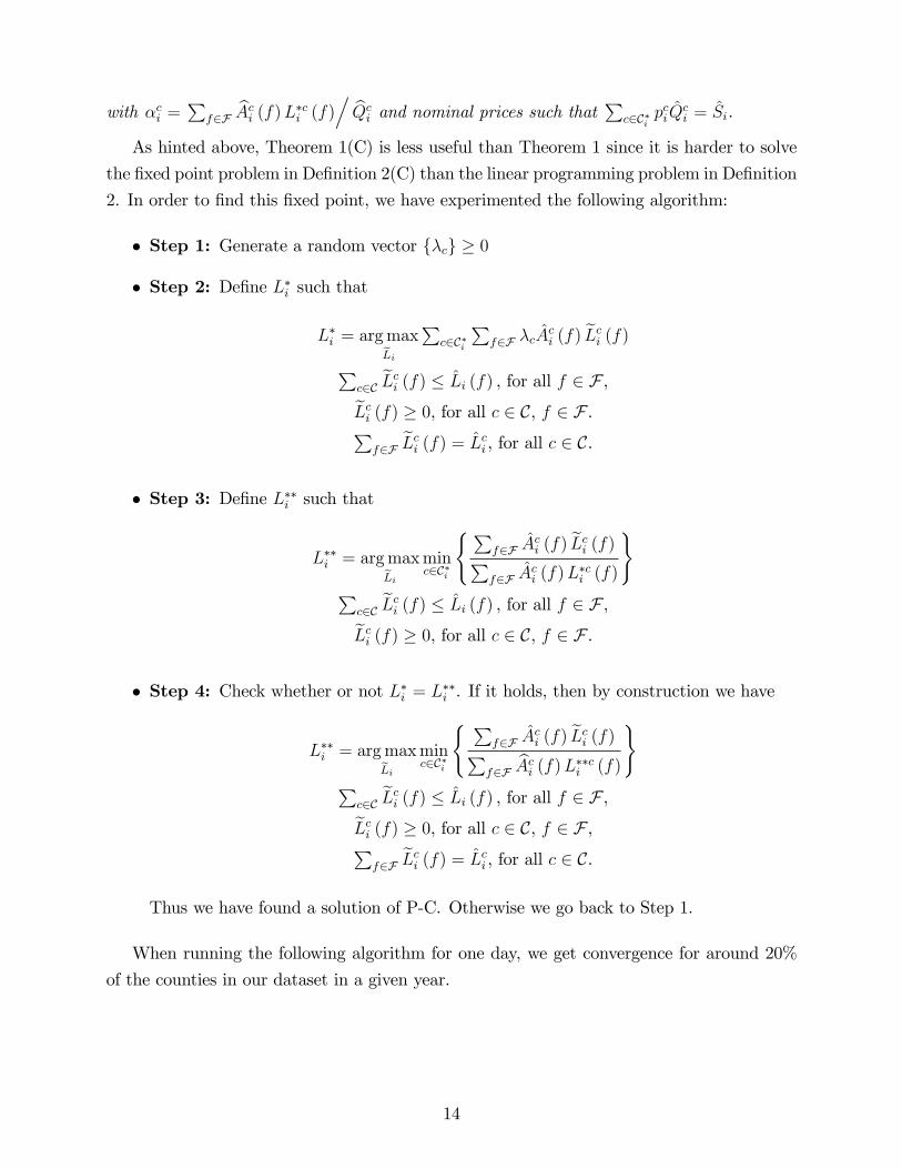
with αci =∑

f∈F Aci (f)L∗ci (f)

/Qci and nominal prices such that

∑c∈C∗i

pciQci = Si.

As hinted above, Theorem 1(C) is less useful than Theorem 1 since it is harder to solve

the fixed point problem in Definition 2(C) than the linear programming problem in Definition

2. In order to find this fixed point, we have experimented the following algorithm:

• Step 1: Generate a random vector {λc} ≥ 0

• Step 2: Define L∗i such that

L∗i = arg maxLi

∑c∈C∗i

∑f∈F λcA

ci (f) Lci (f)∑

c∈C Lci (f) ≤ Li (f) , for all f ∈ F ,

Lci (f) ≥ 0, for all c ∈ C, f ∈ F .∑f∈F L

ci (f) = Lci , for all c ∈ C.

• Step 3: Define L∗∗i such that

L∗∗i = arg maxLi

minc∈C∗i

{∑f∈F A

ci (f) Lci (f)∑

f∈F Aci (f)L∗ci (f)

}∑


Lci (f) ≥ 0, for all c ∈ C, f ∈ F .

• Step 4: Check whether or not L∗i = L∗∗i . If it holds, then by construction we have

L∗∗i = arg maxLi

minc∈C∗i

{ ∑f∈F A

ci (f) Lci (f)∑

f∈F Aci (f)L∗∗ci (f)

}∑


Lci (f) ≥ 0, for all c ∈ C, f ∈ F ,∑f∈F L


Thus we have found a solution of P-C. Otherwise we go back to Step 1.

When running the following algorithm for one day, we get convergence for around 20%

of the counties in our dataset in a given year.

14

6 Concluding Remarks

In this paper we have developed a new approach to measuring the gains from economic inte-

gration based on a Roy-like assignment model in which heterogeneous factors of production

are allocated to multiple sectors in multiple local markets. We have implemented this ap-

proach using data on crop markets in 1,250 U.S. counties from 1840 to 2002. Central to our

empirical analysis is the use of a novel agronomic data source on predicted output by crop

for small spatial units. Crucially, this dataset contains information about the productivity of

all units for all crops, not just those that are actually being grown. Using this new approach

we have estimated (i) the spatial distribution of price wedges across U.S. counties in 1840

and 2002; (ii) the gains associated with changes in the level of these wedges over time; and

(iii) the further gains that could obtain if all wedges were removed and gains from market

integration were fully realized.

15

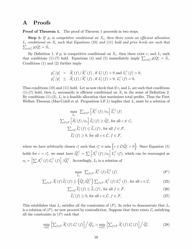
A ProofsProof of Theorem 1. The proof of Theorem 1 proceeds in two steps.

Step 1: If pi is competitive conditional on Xi, then there exists an effi cient allocationLi conditional on Xi such that Equations (10) and (11) hold and price levels are such that∑

c∈C∗ipciQ

ci = Si.

By Definition 1, if pi is competitive conditional on Xi, then there exist ri and Li suchthat conditions (1)-(7) hold. Equations (4) and (5) immediately imply

∑c∈C∗i

pciQci = Si.

Conditions (1) and (2) further imply

pc′


′


i (f) > 0,

pc′


′

i (f) , if Lci (f) > 0, Lc′

i (f) = 0.

Thus conditions (10) and (11) hold. Let us now check that if ri and Li are such that conditions(1)-(7) hold, then Li necessarily is effi cient conditional on Xi in the sense of Definition 2.By conditions (1)-(3), Li is a feasible allocation that maximizes total profits. Thus the FirstWelfare Theorem (Mas-Colell et al. Proposition 5.F.1) implies that Li must be a solution of

maxLi

∑f∈F

[Ac∗ii (f) /αi

]Lc∗ii (f)∑

f∈F

[Aci (f) /αi

]Lci (f) ≥ Qci , for all c 6= c∗i ,∑


Lci (f) ≥ 0, for all c ∈ C, f ∈ F ,

where we have arbitrarily chosen c∗i such that c∗i ≡ min

{c ∈ C|Qci > 0

}. Since Equation (5)

holds for c = c∗i , we must have Qc∗ii =

∑[Ac∗ii (f) /αi

]Lc∗ii (f), which can be rearranged as

αi =[∑

Ac∗ii (f)L

c∗ii (f)

]/Q

c∗ii . Accordingly, Li is a solution of

maxLi

∑f∈F A

c∗ii (f) L

c∗ii (f) (P’)∑

f∈F Aci (f) Lci (f) ≥

(Qci/Q

c∗ii

)∑f∈F A

c∗ii (f)L

c∗ii (f) , for all c ∈ C, (25)∑


Lci (f) ≥ 0, for all c ∈ C, f ∈ F , (27)

This establishes that Li satisfies all the constraints of (P ). In order to demonstrate that Liis a solution of (P ), we now proceed by contradiction. Suppose that there exists L′i satisfyingall the constraints in (P ) such that

minc∈C∗i

[∑f∈F A

ci (f)L

′ci (f)

]/Qcm > min

c∈C∗i

[∑f∈F A

ci (f)Lci (f)

]/Qci . (28)

16

Since Inequality (25) is necessarily binding at a solution of (P ′), we therefore have[∑f∈F A

ci (f)Lci (f)

]/Qci =

[∑f∈F A

c∗ii (f)L

c∗ii (f)

]/Qc∗ii , for all c ∈ C∗i . (29)

Combining Inequality (28) and Equation (29), we obtain[∑f∈F A

ci (f)L

′ci (f)

]/Qci >

[∑f∈F A

c∗ii (f)L

c∗ii (f)


Since L′ci (f) ≥ 0 for all c ∈ C, f ∈ F , we also trivially have

∑Aci (f)L

′ci (f) ≥

(Qci/Q

c∗ii

)∑Ac∗ii (f)L

c∗ii (f) , for all c /∈ C∗i . (31)

By Inequalities (30) and (31), L′i satisfies all the constraints in (P ′). By Inequality (30)evaluated at c = c∗i , we also have[∑

f∈F Ac∗ii (f)L

′c∗ii (f)

]/Qc∗ii >

[∑f∈F A

c∗ii (f)L

c∗ii (f)

]/Qc∗ii .

This contradicts the fact that Li is a solution of (P ′). Thus Li is effi cient conditional on Xi

in the sense of Definition 2. This completes the proof of Step 1.

Step 2: If there exists an effi cient allocation Li conditional on Xi such that Equations(10) and (11) hold and price levels are such that

∑c∈C∗i

pciQci = Si, then pi is competitive

conditional on Xi.

By assumption, the observation Xi is such that Equations (4)-(7) hold. Thus by Def-inition 1, we only need to show that one can construct a vector of field prices, ri, and anallocation of fields, Li, such that conditions (1)-(3) hold as well.A natural candidate for the allocation is Li solution of (P ) such that conditions (10) and

(11) hold. By Definition 2, such a solution exists since there exists an effi cient allocation Liconditional on Xi such that conditions (10) and (11) hold. The fact that Inequality (3) holdsfor allocation Li is immediate from Equation (6) and Inequality (8). Let us now constructthe vector of field prices, ri, such that for

ri (f) = maxc∈C

pciAci (f) Q

c∗ii /[∑

f∈F Ac∗ii (f)L

c∗ii (f)], (32)

with c∗i ≡ min{c ∈ C|Qci > 0

}. Since Equation (5) holds for c = c∗i , Equation (7) implies

αi = [∑

f∈F Ac∗ii (f)L

c∗ii (f)]/Q

c∗ii . Thus we can rearrange Equation (32) as

ri (f) = maxc∈C

pciAci (f) .

This immediately implies Inequality (1). To conclude, all we need to show is that pciAci (f) =

ri (f) if Lci (f) > 0. We proceed by contradiction. Suppose that there exist c ∈ C andf ∈ F such that Lci (f) > 0 and pciA

ci (f) < maxc′∈C p

c′i A

c′i (f). By Equation (7), this can

17

be rearranged as pciAci (f) < maxc′∈C p

c′i A

c′i (f). Now consider c0 = arg maxc′∈C p

c′i A

c′i (f). By

construction, we havepc0i /p

ci > Aci (f) /Ac0i (f) ,

which contradicts either condition (10), if Lc0i (f) > 0, or condition (11), if Lc0i (f) = 0. Thiscompletes the proof of Step 2.

Theorem 1 directly derives from Steps 1 and 2. QED.

Proof of Theorem 1(M). The proof of Theorem 1(M) is similar to the previous proof.

Step 1: If pi is competitive conditional on Yi, then there exists an effi cient allocation Liconditional on Yi such that Equations (10) and (11) hold and price levels are such that∑

c∈C∗ipciQ

ci = Si.

By Definition 1 (M), if pi is feasible conditional on Zi, then there exist ri and Li suchthat (1)-(7) and (14) hold. Equations (4) and (5) immediately imply

∑c∈C∗i

pciQci = Si.

Conditions (1) and (2) further imply

pc′


′


i (f) > 0,

pc′


′

i (f) , if Lci (f) > 0, Lc′

i (f) = 0.

Thus conditions (10) and (11) hold. Let us now check that if ri and Li are such that conditions(1)-(7) hold, then Li necessarily is effi cient conditional on Xi in the sense of Definition 2 (M).By conditions (1)-(3), Li is a feasible allocation that maximizes total profits. Thus the FirstWelfare Theorem (Mas-Colell et al. Proposition 5.F.1) implies that Li must be a solution of

maxLi

∑f∈F

[Ac∗ii (f) /αi

]Lc∗ii (f)∑

f∈F

[Aci (f) /αi


f∈F Ami L

mi (f) ≥ Qmi ,∑

j∈C∪{m} Lji (f) ≤ Li (f) , for all f ∈ F ,

Lji (f) ≥ 0, for all j ∈ C∪{m} , f ∈ F ,


{c ∈ C|Qci > 0

}. Since Equation

(5) holds for c = c∗i , we must have Qc∗ii =

∑[Ac∗i (f) /αi

]Lc∗i (f), which can be rearranged

αi =[∑

Ac∗i (f)Lc

∗i (f)

]/Q

c∗ii . By Equation (14) we must also have Qmi = Ami L

mi . Thus we

18

can rearrange the previous program as

maxLi

∑f∈F A

c∗ii (f) L

c∗ii (f) (P-M’)∑

f∈F Aci (f) Lci (f) ≥

(Qci/Q

c∗ii

)∑f∈F A

c∗ii (f)L

c∗ii (f) , for all c ∈ C, (33)∑

f∈F Lmi (f) ≥ Lmi , (34)∑

j∈j∈C∪{m} Lji (f) ≤ Li (f) , for all f ∈ F , (35)

Lji (f) ≥ 0, for all j ∈ C∪{m} , f ∈ F . (36)

This establishes that Li satisfies all the constraints of (P −M). In order to demonstratethat Li is a solution of (P −M), we now proceed by contradiction. Suppose that there existsL′i satisfying all the constraints in (P −M) such that

minc∈C∗i

[∑f∈F A

ci (f)L

′ci (f)

]/Qcm > min

c∈C∗i

[∑f∈F A

ci (f)Lci (f)

]/Qci . (37)

Since Inequality (P −M ′) is necessarily binding at a solution of (P −M ′), we therefore have[∑f∈F A

ci (f)Lci (f)

]/Qci =

[∑f∈F A

c∗ii (f)L

c∗ii (f)


Combining Inequality (37) and Equation (38), we obtain[∑f∈F A

ci (f)L

′ci (f)

]/Qci >

[∑f∈F A

c∗ii (f)L

c∗ii (f)


Since L′ci (f) ≥ 0 for all c ∈ C, f ∈ F , we also trivially have

∑Aci (f)L

′ci (f) ≥

(Qci/Q

c∗ii

)∑Ac∗ii (f)L

c∗ii (f) , for all c /∈ C∗i . (40)

By Inequalities (39) and (40), L′i satisfies all the constraints in (P −M ′). By Inequality (39)evaluated at c = c∗i , we also have[∑

f∈F Ac∗ii (f)L

′c∗ii (f)

]/Qc∗ii >

[∑f∈F A

c∗ii (f)L

c∗ii (f)

]/Qc∗ii .

This contradicts the fact that Li is a solution of (P −M ′). Thus Li is effi cient conditionalon Yi in the sense of Definition 1 (M). This completes the proof of Step 1.

Step 2: If there exists an effi cient allocation Li conditional on Yi such that Equations(10) and (11) hold and price levels are such that

∑c∈C∗i


conditional on Yi.

By assumption, the observation Yi is such that Equations (4)-(7) and (14) hold. Thusby Definition 1 (M), we only need to show that one can construct a vector of field prices, ri,and an allocation of fields, Li, such that conditions (1)-(3) hold as well.A natural candidate for the allocation is Li solution of (P −M) such that conditions

19

(10) and (11) hold. By Definition 2 (M), such a solution exists since there exists an effi cientallocation Li conditional on Yi such that conditions (10) and (11) hold. The fact thatInequality (3) holds for allocation Li is immediate from Equation (6) and Inequality (15).Let us now construct the vector of field prices, ri, such that for

ri (f) = maxc∈C

pciAci (f) Q

c∗ii /[∑

f∈F Ac∗ii (f)L

c∗ii (f)], (41)


}. Since Equation (5) holds for c = c∗i , Equation (7) implies

αi = [∑

f∈F Ac∗ii (f)L

c∗ii (f)]/Q

c∗ii . Thus we can rearrange Equation (41) as

ri (f) = maxc∈C

pciAci (f) .

This immediately implies that Inequality (1) holds for all c ∈ C. To conclude, all we needto show is that pciA

ci (f) = ri (f) if Lci (f) > 0. We proceed by contradiction. Suppose

that there exist c ∈ C and f ∈ F such that Lci (f) > 0 and pciAci (f) < maxc′∈C p

c′i A

c′i (f).

By Equation (7), this can be rearranged as pciAci (f) < maxc′∈C p

c′i A

c′i (f). Now consider

c0 = arg maxc′∈C pc′i A

c′i (f). By construction, we have

pc0i /pci > Aci (f) /Ac0i (f) ,


Theorem 1(M) directly derives from Steps 1 and 2. QED.

Proof of Theorem 1(C). The proof of Theorem 1(C) is similar to the previous proofs.

Step 1: If pi is competitive conditional on Zi, then there exists an effi cient allocationLi conditional on Zi such that Equations (10) and (11) hold and price levels are such that∑

c∈C∗ipciQ

ci = Si.

By Definition 1(C), if pi is competitive conditional on Zi, then there exist ri and Lisuch that conditions (1)-(6) and (19)-(18) hold. Equations (4) and (5) immediately imply∑

c∈C∗ipciQ

ci = Si. Conditions (1) and (2) further imply

pc′

i /pci = Aci (f)αc

′

i /Ac′


′

i (f) > 0,

pc′

i /pci ≤ Aci (f)αc

′

i /Ac′

i (f)αci , if Lci (f) > 0, Lc

′

i (f) = 0.

Thus conditions (23) and (24) hold. Let us now check that if ri and Li are such thatconditions (1)-(6) and (19)-(18) hold, then Li necessarily is effi cient conditional on Zi in thesense of Definition 2(C). By conditions (1)-(3), Li is a feasible allocation that maximizes totalprofits. By Equation (19), it also satisfies

∑f∈F L

ci (f) = Lci . Thus, by the First Welfare

20

Theorem (Mas-Colell et al. Proposition 5.F.1), Li must be a solution of

maxLi

∑f∈F

[Ac∗ii (f) /αci

]Lc∗ii (f)∑

f∈F

[Aci (f) /αci



Lci (f) ≥ 0, for all c ∈ C, f ∈ F ,∑f∈F L



{c ∈ C|Qci > 0

}. Since Equation

(5) holds for all c, we must have Qci =∑

[Aci (f) /αci ]Lci (f), which can be rearranged as

αci = [∑Aci (f)Lci (f)] /Qci for all c ∈ C∗i . Accordingly, Li is a solution of

maxLi

∑Ac∗ii (f) L

c∗ii (f) (P-C’)∑

Aci (f) Lci (f) ≥∑Aci (f)Lci (f) , for all c 6= c∗i , (42)∑


Lci (f) ≥ 0, for all c ∈ C, f ∈ F , (44)∑f∈F L

ci (f) = Lci , for all c ∈ C. (45)

This establishes that Li satisfies all the constraints of (P − C). In order to demonstrate thatLi is a solution of (P − C), we now proceed by contradiction. Suppose that there exists L′isatisfying all the constraints in (P − C) such that

minc∈C∗i

{∑f∈F A

ci (f)L′ci (f)∑


}> min

c∈C∗i

{∑f∈F A

ci (f)Lci (f)∑


}= 1. (46)

Inequality (46) immediately implies∑f∈F A

ci (f)L′ci (f) >

∑f∈F A

ci (f)Lci (f) for all c ∈ C∗i . (47)

Since Li is such that Equation (5) holds for all c, we also know that Lci (f) = 0 for allf ∈ F ,c /∈ C∗i . Since L

′ci (f) ≥ 0 for all c ∈ C, f ∈ F , we also trivially have∑Aci (f)L

′ci (f) ≥

∑Aci (f)Lci (f) , for all c /∈ C∗i . (48)

By Inequalities (47) and (48), L′i satisfies all the constraints in (P − C ′). By Inequality (47)evaluated at c = c∗i , we also have∑

f∈F Ac∗ii (f)L

′c∗ii (f) >

∑f∈F A

c∗ii (f)L

c∗ii (f) .

21

This contradicts the fact that Li is a solution of (P − C ′). Thus Li is effi cient conditionalon Zi in the sense of Definition 2(C). This completes the proof of Step 1.

Step 2: If there exists an effi cient allocation Li conditional on Zi such that Equations(23) and (24) hold and price levels are such that

∑c∈C∗i


conditional on Zi.

By assumption, the observation Zi is such that Equations (4)-(6) and (19)-(18) hold.Thus by Definition 1(C), we only need to show that one can construct a vector of fieldprices, ri, and an allocation of fields, Li, such that conditions (1)-(3) hold as well.A natural candidate for the allocation is Li solution of (P − C) such that conditions

(23) and (24) hold. By Definition 2(C), such a solution exists since there exists an effi cientallocation Li conditional on Zi such that conditions (23) and (24) hold. The fact thatInequality (3) holds for allocation Li is immediate from Equation (6) and Inequality (20).Let us now construct the vector of field prices, ri, such that for

ri (f) = maxc∈C∗i

pciAci (f) Qci/[

∑f∈F A

ci (f)Lci (f)], (49)


}. Since Equation (5) holds for all c, Equation (18) implies

αci = [∑

f∈F Aci (f)Lci (f)]/Qci for all c ∈ C∗i . Thus we can rearrange Equation (49) as

ri (f) = maxc∈C∗i

pciAci (f) .

Under the assumption C = C∗i , this immediately implies Inequality (1). To conclude, all weneed to show is that pciA

ci (f) = ri (f) if Lci (f) > 0. We proceed by contradiction. Suppose

that there exist c ∈ C and f ∈ F such that Lci (f) > 0 and pciAci (f) < maxc′∈C∗i p

c′i A

c′i (f).

By Equation (18), this can be rearranged as pciAci (f) /αci < maxc′∈C p

c′i A

c′i (f) /αc

′i . Now

consider c0 = arg maxc′∈C pc′i A

c′i (f) /αc

′i . By construction, we have

pc0i /pci > Aci (f)αc0i /A

c0i (f)αci ,


Theorem 1(C) directly derives from Steps 1 and 2. QED.

22

ReferencesChetty, Raj (2009), “Suffi cient Statistics for Welfare Analysis: A Bridge Between Structural

and Reduced-Form Methods,”Annual Review of Economics, 1, pp. 451-488.

Costinot, Arnaud (2009), “An Elementary Theory of Comparative Advantage,”Economet-rica, 77(4), pp. 1165-1192.

Eaton, Jonathan and Samuel Kortum (2002), “Technology, Geography and Trade,”Econo-metrica, 70(5), pp. 1741-1779.

Frankel, Jeffrey A. and David Romer, “Does Trade Cause Growth?,”American EconomicReview, 89(3), pp. 379-399.

Hsieh, Chang-Tai and Pete Klenow (2009), Misallocation and Manufacturing TFP in Chinaand India, Quarterly Journal of Economics, 124(4), pp. 1403-1448

Waugh, Michael (2010), “International Trade and Income Differences,”American EconomicReview, 100(5), pp. 2093-2124.

23

Documents

How Large are the Gains from Economic Integration? …ies/IESWorkshopS2011/DonaldsonPaper.pdfHow Large are the Gains from Economic Integration? Theory and Evidence from U.S ... ment