Board of Governors of the Federal Reserve System

International Finance Discussion Papers

Number 935

July 2008

How Long Can the Unsustainable U.S. Current Account Deficit Be Sustained?

Carol C. Bertaut, Steven B. Kamin, and Charles P. Thomas

NOTE: International Finance Discussion Papers are preliminary materials circulated to stimulate discussion and critical comment. References in publications to International Finance Discussion Papers (other than an acknowledgment that the writer has had access to unpublished material) should be cleared with the author or authors. Recent IFDPs are available on the Web at www.federalreserve.gov/pubs/ifdp/. This paper can be downloaded without charge from Social Science Research Network electronic library at http://www.ssrn.com/.

How Long Can the Unsustainable U.S. Current Account Deficit Be Sustained?

Carol C. Bertaut, Steven B. Kamin, and Charles P. Thomas*

July 2008

Abstract: This paper addresses three questions about the prospects for the U.S. current account deficit. Is it sustainable in the long term? If not, how long will it take for measures of external debt and debt service to reach levels that could prompt some pullback by global investors? And if and when such levels are breached, how readily would asset prices respond and the current account start to narrow? To address these questions, we start with projections of a detailed partial-equilibrium model of the U.S. balance of payments. Based on plausible assumptions of the key drivers of the U.S. external balance, they indicate that the current account deficit will resume widening and the negative NIIP/GDP ratio will continue to expand. However, our projections suggest that even by the year 2020, the negative NIIP/GDP ratio will be no higher than it is in several industrial economies today, and U.S. net investment income payments will remain very low. The share of U.S. claims in foreigners’ portfolios will likely rise, but not to an obviously worrisome extent. All told, it seems likely it would take many years for the U.S. debt to cumulate to a level that would test global investors’ willingness to extend financing. Finally, we explore the historical responsiveness of asset prices and the current account in industrial economies to measures of external imbalances and debt. We find little evidence that, as countries’ net indebtedness rises, the developments needed to correct the current account—including changes in growth rates, asset prices, or exchange rates—materialize all that rapidly. We would emphasize that these findings do not imply that U.S. current account adjustment is necessarily many years away, as any number of factors could trigger such adjustment. Our point is rather that international balance sheet considerations likely are not sufficient, by themselves, to require external adjustment any time soon. JEL Codes: F21, F32, F37

Keywords: sustainability, external imbalance, dollar

*The authors are economists in the International Finance Division of the Federal Reserve Board. They can be reached at carol.bertaut@frb.gov, steven.kamin@frb.gov , and charles.thomas@frb.gov. This paper has benefitted from comments by Trevor Reeve and participants at the Current Account Sustainability in Major Economies (II) conference at the University of Wisconsin, especially our discussant Jeffrey Frankel. The views in this paper are solely the responsibility of the authors and should not be interpreted as reflecting the views of the Board of Governors of the Federal Reserve System or of any other person associated with the Federal Reserve System. Jim Albertus, Sean Fahle and Dao Nguyen provided excellent research assistance.

1

I. Introduction and Summary

Several years ago, as the U.S. current account deficit was expanding to record levels,

observers increasingly began to focus on the unsustainability of the U.S. external imbalances, as

well as the possibility that the subsequent correction would be abrupt and disorderly.1 Since

peaking at 6.6 percent of GDP in the third quarter of 2006, however, the current account deficit

has begun shrinking as a result of declines in the foreign exchange value of the dollar, slower

U.S. GDP growth, and continued strong expansion abroad; the deficit dipped to 4.9 percent in

the fourth quarter of 2007. With the reduction in the deficit and the depreciation of the dollar,

which in real multilateral terms is now about 25 percent below its peak level in February 2002,

concerns about a disorderly correction appear to have become less prominent. This may in part

reflect a growing conviction that a correction of the current account is likely to be orderly rather

than disruptive.2 It may also reflect a view that, with recent declines in the dollar and in the

deficit, no further correction of the U.S. current account may be necessary.

In this paper, we address three simple questions: Is the U.S. current account now

sustainable on a long-term basis? If not, how long might it take for measures of U.S. external

indebtedness to expand beyond levels that global investors are willing to finance? And finally, if

and when such levels are breached, how rapidly might a correction in asset prices and the current

account ensue?

We start, in Section II, by discussing the most common metric for assessing current

account sustainability, the stability of an economy=s net debt as a share of GDP; such stability is

necessary if net interest payments to foreigners are not to rise without limit as a share of income.

1See, among others, Edwards (2005), Eichengreen (2004), Mann (1999, 2002, 2003), Mussa (2004), Obstfeld and Rogoff (2004), Roubini and Setzer (2004), and Truman (2004). 2 Freund (2005), Croke, Kamin, and Leduc (2006), Gagnon (2005), and Debelle and Galati (2005), among others, present evidence suggesting that current account corrections in industrial economies have generally been benign.

2

We go on in Section III to describe projections of U.S. external balance variables and measure

them against the sustainability criterion described above. The projections are based on

simulations of a detailed model of the U.S. balance of payments, taking as exogenous the key

drivers of the U.S. trade and current accounts: GDP growth in the United States and abroad,

inflation rates, interest rates, oil prices, and the level of the real multilateral dollar. We find that,

based on our model simulations, beyond the near term, the current account deficit likely will

begin widening again and U.S. external debt will rise steadily.

However, just because the current account is unsustainable in the long term does not

mean that a correction is imminent. Theory provides no guidance as to how large the external

debt must become before developments are triggered that would narrow the U.S. current account

deficit. Our baseline projection suggests that the U.S. net external debt will grow from around

20 percent of GDP at present to around 60 percent of GDP by 2020. Is that a lot or a little? To

answer this question, we look to the current pattern of external liabilities among industrial

countries, and we find a number of countries whose external debt ratios currently are 60 percent

or higher.

The net debt/GDP ratio, while a common and useful summary measure of an economy=s

international balance-sheet situation, is not a perfect or unique indicator of a country=s

creditworthiness. Accordingly, in Section IV, we consider a second metric of current account

sustainability: the exposure of investors to U.S. assets in terms of the share of U.S. securities in

foreign portfolios. If the financing of the current account deficit means that this exposure is

rising without limit, that, too, would suggest that the current account is unsustainable. We find

no evidence that, to date, the exposure of foreign investors to U.S. assets has been rising.

Calculations based on our projections of the U.S. balance of payments (described above) suggest

that this exposure will increase going forward, but not necessarily to a worrisome extent.

3

All told, the evidence we present in Sections III and IV suggests that, even in the absence

of further changes in the driving variables, it would likely be many years before indicators of the

U.S. international balance sheet breached any significant thresholds of creditworthiness and

investor exposure. Yet, if such thresholds were breached, do we know how rapidly forces would

be set in motion to narrow the current account deficit and restrain the growth of external debt?

To address this question, Section V examines the extent to which, historically, higher levels of

external debt or related imbalances have led to changes in an economy=s access to financing. We

first examine the effect of external debt on two variables that closely reflect the behavior of

global investors: interest rates and exchange rates. Estimating panel regressions for a sample of

industrial countries, we find that higher levels of debt push up interest rates in a country by only

a very small extent, and exert no discernable effect on exchange rates. We then reproduce

recent results by Gruber and Kamin (2008), who find that in panel regressions to explain the

current account balance, the lagged value of the net international investment position (NIIP)

invariably has a positive and significant coefficient; this suggests that higher levels of debt lead

to larger, not smaller, current account deficits. Section VI summarizes our findings and

advances some tentative conclusions.

II. Assessing Current Account Sustainability

II.1 The NIIP/GDP criterion

The net international investment position (NIIP) represents the sum of all claims by U.S.

residents on foreign residents less the claims of foreigners on the United States. The NIIP is a

key determinant (along with rates of return) of U.S. net investment income: the sum of receipts

on foreign assets owned by U.S residents net of payments on foreign claims on U.S. residents.

Therefore, most analysts underscore that a necessary condition for current account sustainability

4

is that the NIIP/GDP ratio be stable (Mann, 1999, 2002, 2003, Mussa, 2004, Cline, 2005,

Edwards, 2005). Otherwise, if the (negative) NIIP/GDP ratio were to rise without limit, the ratio

of net investment payments to GDP would rise as well, and would eventually exceed GDP.

Unrestrained increases in the (negative) NIIP/GDP ratio beyond some threshold should

set in train a number of developments that would narrow the current account deficit and restrain

the growth of external debt: U.S. residents would reduce their spending as their wealth declined

and they experienced an erosion of the amount of disposable income remaining after servicing

their debt. And foreigners would sell off U.S. assets as they became concerned about our ability

to repay debts, weakening the dollar and thus again leading to smaller deficits.

The stability of the NIIP/GDP ratio required for current account sustainability, in turn,

imposes limits on the current account deficit. To see this, note that for the ratio of the NIIP to

GDP to remain stable over time, the proportionate change in the NIIP must equal the

proportionate rise in nominal GDP:

(NIIPt - NIIPt-1)/NIIPt-1 = (GDPt - GDPt-1)/GDPt-1

Leaving aside any valuation adjustments, the annual change in the NIIP is equal to the current

account balance:

NIIPt - NIIPt-1 = Current Accountt

Therefore the proportionate change in the NIIP is equal to the ratio of the current account to the

lagged NIIP; this, in turn, approximately equals the current account/GDP ratio divided by the

NIIP/GDP ratio:

(NIIPt - NIIPt-1)/NIIPt-1 = (Current Accountt /NIIPt-1)

. (Current Accountt /GDPt)/(NIIPt/GDPt)

5

Accordingly, for the ratio of the NIIP to GDP to remain stable over time, the current

account/GDP ratio divided by the NIIP/GDP ratio must equal the proportionate rise in nominal

GDP:

(Current Accountt /GDPt)/(NIIPt/GDPt) . (GDPt - GDPt-1)/GDPt

In 2007, the current account deficit was about 5 percent of GDP and the NIIP was about -

18 percent of GDP. This implies, all else held constant, that the NIIP would rise (become more

negative) at a pace of 28 percent annually, much faster than the prospective rate of increase of

nominal GDP of 4.4 percent (see Section III). Were the current account deficit to remain at 5

percent of GDP, the NIIP/GDP ratio would stabilize once it reached -114 percent.3 This is

because at that level of the NIIP, the proportionate rise in the NIIP–5 percent/114 percent–is

equal to the prospective 4.4 percent rise in nominal GDP. How large a negative NIIP/GDP ratio

is sustainable? Nobody knows, but some relevant considerations are discussed in Section III.4.

II.2 Qualifications to the NIIP as a measure of external sustainability

The NIIP does not fully summarize the sustainability of the external position. As will be

discussed further below, depending upon the rate of return, the same NIIP may be associated

with very different net investment income flows. Several additional considerations also affect

the interpretation of the NIIP as a measure of creditworthiness and sustainability.

First, changes in the valuation of assets may affect the NIIP without affecting the

economy=s underlying capacity to service the external position. For example, all else equal, a

rise in U.S. stock prices will raise the value of foreign holdings of U.S. assets and thus cause the

NIIP to become more negative. However, this does not necessarily mean that the U.S. external

3 This discussion leaves open the question of what level of the trade balance would be needed to achieve the level of the current account required to stabilize the NIIP/GDP ratio. One rule of thumb is that current account stability requires the trade balance to be equal to zero; then, the current account equals net income payments on the NIIP, the NIIP grows at the rate of interest, and, if GDP grows at the rate of interest as well, the NIIP/GDP ratio is stabilized.

6

position has become more difficult to finance. On the contrary, the higher stock prices may

reflect increases in U.S. income and productivity, raising our capacity to make foreign payments;

moreover, higher stock prices mean we can finance the same current account deficit through the

sale of fewer (but pricier) equities to foreigners.

An extreme example of the impact of equity valuations on the NIIP is Finland, where a

substantial share of its external liabilities consists of foreign holdings of stock in Nokia. As

shown in the top panel of Exhibit 1, the surge in the NIIP to nearly -170 percent of GDP in 1999

was driven by a parallel surge in the price of Nokia stock, and when that stock declined, so, too,

did the size of Finland=s negative NIIP.

Second, and as a related point, one should not confuse the NIIP with the net wealth of an

economy’s residents. Net wealth is comprised of total assets owned by residents, both domestic

and foreign, less foreigners’ claims on those residents. The bottom panel of Exhibit 1 compares

the net wealth of U.S. residents to the NIIP (expressed as a liability position) and total gross

claims on U.S. residents, including foreign direct investment in the United States. (It is

important to note that in this measure of net wealth the foreign claims, or net liabilities, have

already been netted out.) As the chart illustrates, relative to net wealth both the U.S. net debt

position and the gross claims of foreigners remain relatively small.4 Presumably, a country=s

ability to repay external debt will depend not only on its GDP, but also on its total wealth, just as

a homeowner=s ability to repay his mortgage depends not just on his income, but on the value of

his assets including, but not limited to, his house. Accordingly, increases in net external debt

accompanied by even larger increases in the value of domestic assets should not lead to

correction of the current account deficit: there should not be declines in creditworthiness leading

4 See, also, Xafa (2007).

7

to a pullback for global investors, nor should the rising debt lead to spending restraint by U.S.

residents as long as total wealth is rising.

Finally, the aggregate NIIP may be only loosely related to the credit risk that foreign

investors face. In principle, the creditworthiness of a borrower is determined by, among other

things, the total debt the borrower has issued. For most international borrowers in an industrial

economy, however, foreigners represent only a small portion of their creditor base, with most

liabilities being to domestic residents. Therefore, the fact that foreign claims on the United

States are rising does not necessarily mean that U.S. indebtedness is rising relative to its ability

to repay. The diversity and distribution of creditworthiness across borrowers in a given economy

is likely to influence the credit risks faced by foreign investors to a greater degree than the

overall foreign indebtedness of the economy. (As discussed in more detail in Section III.5, the

riskiness of U.S. external debt is reduced by the fact that the major debtor is the U.S.

government.) This is reinforced by the fact that in most industrial countries, it is not possible to

treat foreign creditors differently from domestic creditors.

III. Simulations of the U.S. balance of payments

With these qualifications in mind, we now consider projections of the U.S. balance of

payments to determine whether the key criterion for current account sustainabilityBthe stability

of the NIIP/GDP ratioBis likely to be met. For this exercise, we use the Federal Reserve Board=s

partial-equilibrium model of the balance of payments, which is described briefly below. (A more

complete description is provided at the end of this paper.)

Before proceeding, we address the desirability of using a partial equilibrium model—

which assumes the key macroeconomic drivers of the current account to be exogenous—to

assess current account sustainability. In principle, the new generation of forward-looking

8

dynamic general equilibrium models might be better suited for longer run macroeconomic

projections. However, in these models, trade deficits and external debt represent equilibrium

responses to shocks, and asset prices and deficits start to correct long before economies reach

any putative debt limits. (See, for example, Erceg, Guerrieri, and Gust, 2006) Conversely,

much of the debate over U.S. external sustainability assumes that U.S. indebtedness may expand

until it reaches certain limits, after which correction may be triggered. In this context, it makes

sense to use a partial equilibrium model, which does not assume spending adjusts endogenously

in response to future financing constraints, to forecast the paths of external imbalances and debt

under plausible assumptions about output growth and prices, and then to assess whether those

paths are sustainable. Moreover, the USIT partial-equilibrium model described below treats the

U.S. balance of payments in considerably more detail than any general equilibrium model

currently in use, and such detail is essential to assessing current account sustainability.

III.1 The USIT model

The USIT (U.S. International Transactions) model consists of 491 equations including 26

econometrically estimated behavioral equations, with the rest being identities and other

computational equations. The model takes as exogenous projections for the central determinants

of the U.S. external accounts, including: U.S. and foreign real GDP growth, U.S. and foreign

inflation rates, U.S. interest rates, oil prices, and the foreign exchange value of the dollar. Based

on these inputs, it then projects U.S. external balance variables in four broad categories: (1) trade

flows, (2) non-trade components of the current account (especially investment income), (3)

financing flows, and (4) the investment positions comprising the NIIP. Salient aspects of the

modeling strategy and parameters are as follows:

9

(1) Trade sector

• Import prices for most major categories are projected based on the level of the dollar, foreign CPIs, and the U.S. CPI; the rate of passthrough from changes in the dollar to changes in merchandise import prices is quite low, about 1/3. Export prices depend on measures of U.S. production costs and final prices.

• Real imports for most major categories depend on both the prices of imports relative to

U.S. pricesBwith an elasticity of about unityBand on U.S. GDP. Real exports for most major categories depend on the price of exports relative to exchange-rate-converted foreign CPIsBalso with an elasticity of about unityBand on a trade-weighted aggregate of foreign GDPs. Importantly, these equations incorporate the Houthakker-Magee asymmetry in income elasticities: the elasticity of real imports with respect to U.S. GDP is about 1.75 on average, exceeding the elasticity of real exports with respect to foreign GDP, of about 1.25 on average.5

• Both the quantity and price of oil imports are modeled separately, with the former based

on trends in U.S. production and consumption of oil, and the latter based on current and prospective market developments.

(2) Non-trade components of the current account balance

• Investment income is projected by applying income rates of return to different categories of U.S. external claims and liabilities.

• Assumptions on U.S. interest rates are used to project income rates on portfolio (equity,

bond and deposit) positions. Skipping ahead slightly to Exhibit 2, the rates of income on U.S. private portfolio assets and liabilities have been roughly similar in recent years and are projected to remain so, at a level close to the projected U.S. short-term rate of interest, going forward. The income return on Government liabilities has been somewhat higher (closer to the long-term rate of interest) and is projected to remain somewhat higher than the private rates of return.

• The income rate of return on foreign direct investment in the United States depends on the U.S. output gap. The rate of return on U.S. direct investment abroad depends on the foreign output gap and the relative price of oil.

• Historically, income rates on U.S. direct investment abroad have exceeded that on foreign

direct investment in the United States. Although this gap has narrowed over the past decade, it remains large and we project it to remain large in the future.6

5 The theoretical basis for the Houthakker-Magee asymmetry remains ambiguous and the subject of controversy among trade modelers. Even so, the estimated coefficients in our trade models continue to exhibit the Houthakker-Magee asymmetry for goods trade. For services trade, in contrast, the income elasticity for exports exceeds that for imports. However, as goods trade exceeds services trade, the income elasticity for total imports exceeds that of total exports.

6 A number of explanations have been advanced for the asymmetry of rates of return on direct investment, including

10

• Transfers are projected exogenously, based on recent trends.

(3) Financing Flows

• Once the current account balance is projected, this pins down the amount of net financing flows into (out of) the U.S. economy. However, two additional facets of these flows must be specified. First, financial flows must be allocated among the various categories: direct investment and portfolio investment. Second, a given amount of net financing may be associated with any number of combinations of gross financing flows. For example, an $800 billion net inflow may be achieved by $800 billion in gross inflows from abroad, combined with 0 outflows; or it could be achieved by $1,600 billion in gross inflows and $800 billion in gross outflows.

• Gross direct investment flows to/from the United States depend on GDP growth in the

recipient country.

• Foreign flows into U.S. government assets and U.S. government flows into foreign assets are projected at their recent trends.

• This leaves net private portfolio flows to balance the current account/financial account identity. The gross flows are constructed so as to produce growth rates in the stock of claims and liabilities that most closely match recent history while still having the implied net flows meet the net financing requirement.7

(4) Investment positions

• For each category of investment (direct investment, private portfolio, government portfolio, etc.), the gross asset or liabilities position in a given year will be equal to the position in the preceding year plus (a) financial flows (positive or negative) in that category during the year, and (b) valuation changes in the position.

• For all the simulation exercises, we report the direct investment positions and the NIIP using the current cost measure of direct investment.8

• In the simulation projections presented here, we include valuation changes to the direct

investment positions alone, not the portfolio positions. The valuation changes for the greater efficiency of U.S. firms, better project selection by U.S. firms, younger and thus less mature investments for foreign firms in the United States, greater competitive pressures in the U.S. market, or differences in tax treatment. (See Higgins, Klitgaard, and Tille, 2005.) None of these factors seem likely to disappear in the near term. 7 This is accomplished by starting out with trend extrapolations of gross inflows and outflows. If more financing is needed, gross inflows are adjusted up and outflows are adjusted down symmetrically; the reverse occurs if less financing is needed. 8 This is BEA’s preferred measure as it avoids many methodological issues associated with estimating the stock market value of non-traded equity positions. In addition, for our simulations, using the current cost measure means our estimates do not depend on our assumptions about future stock market movements.

11

direct investment positions reflect changes in exchange rates and in domestic prices of the assets (land, machinery, structures, etc.) comprising the position.

III.2 Key assumptions for the projection

The most important assumptions underlying the baseline balance-of-payments projection

are shown on the first page of exhibit 2.

• The real multilateral exchange value of the dollar is held constant at its level at the beginning of 2008.

• For U.S. real GDP growth, rates in 2008 and 2009 are based on OECD projections, while

longer-term growth rates of 2.4 percent are based on the OECD assessment of U.S. potential GDP growth in 2009 (OECD, 2008). In between the near term and farther out, growth jumps temporarily to restore the actual level of GDP to potential, after which growth subsides to its potential rate and the output gap remains at zero.

• GDP growth in the foreign industrial economies is projected in the same manner, based

on OECD (2008). GDP growth in developing countries is based on the IMF=s World Economic Outlook projections for 2008, on the average growth rate from 1997-2007 for further out, and also incorporates a transitional period to restore levels of GDP to their potential levels.

• For 2008 and 2009, U.S. long- and short-term interest rates are based on OECD (2008).

Beyond a transitional period, long-term rates are set equal to the projected growth of nominal GDP: real growth of 2.4 percent plus inflation of 2 percent, based on the OECD 2009 projection. Short-term rates are set 1 percentage point below long-term rates.

• The price of imported oil is set flat at its value at the beginning of this year. Note that

imported oil is comprised of a mix of different grades, and its price is accordingly lower than that of West Texas Intermediate, whose price approached $100 per barrel around that time.

III.3 Model projections The baseline projection

As indicated in the second page of Exhibit 2, after some initial wiggles, real exports grow

at a pace of nearly 5 percent over most of the projection period. Real imports, reflecting their

higher elasticity with respect to GDP, grow a touch faster than 5 percent. In consequence, the

trade balance widens gradually as a share of GDP, reaching about 52 percent by 2020. The non-

oil trade deficit expands at a faster pace, as the volume of oil imports rises more slowly than

12

other types of imports, consistent with trend declines in the oil-intensity of U.S. GDP.9 The

current account balance also declines gradually as a share of GDP, reflecting not only the

widening trade deficit, but also a (long-expected) shift in the balance on investment income from

positive to negative as the NIIP gets more negative; net investment income and the current

account deficit would deteriorate even faster were it not for the asymmetry in the rates of return

on foreign direct investment. Finally, reflecting all of these developments, the NIIP/GDP ratio

deteriorates steadily over the projection period, reaching over -60 percent of GDP by 2020.

Because of their importance for net investment income and thus the current account

balance, the third page of Exhibit 2 provides more detail on the composition of projected gross

investment positions and on the rates of return on these positions. The bottom panel indicates

that the high rates of return on direct investment claims that we are assuming is well in line with

past history, while the rate of return on direct investment liabilities is, if anything, generous by

historical standards. The similarity in our projection of rates of return on portfolio claims and

liabilities is also supported by history. The top panel shows that increases in U.S. direct

investment claims, which have the potential to significantly improve the net investment income

balance owing to their high rate of return, do not appear out of line with the evolution of other

categories.

We draw four central conclusions from this projection. First, based on the standard

criterionBstability of the NIIP/GDP ratioBthe U.S. current account balance is not sustainable in

the long term. The NIIP/GDP ratio deteriorates by more than 40 percentage points of GDP by

2020, or very roughly 4 percentage points per year. But, second, even if the current account is

unsustainable, it is probably less unsustainable than would have been the case had we started the

9 The saw-toothed pattern of the trade balance is caused by a residual seasonal pattern (even after seasonal adjustment by BEA) in oil imports.

13

projection back in, say, 2000; at that time, as indicated in the first page of Exhibit 2, the real

value of the dollar was considerably higher, and U.S. and foreign growth seemed more similar.

Moreover, and third, it is doubtful that, by 2020, the U.S. balance of payments will be entering

any Adanger zone@ where external adjustment will be urgently required. Although the level of the

net debt appears quite elevated (this will be discussed further below), net investment income

payments still represent a paltry 2 percentage point of GDP. This debt burden implies only a

minimal drag on spending, nor would it wave a red flag to investors concerned about the

creditworthiness of the U.S. economy. Fourth and finally, even if investors took more signal

from the NIIP/GDP ratio than from the net investment income balance, it would take quite a few

years before the net debt rose above 60 percent of GDP.

As in all forecasts, our projections depend crucially on the extrapolation of past

relationships and parameters into the future. We would note that two of our most important such

extrapolations have opposite effects on the outlook. On the one hand, our assumption that the

Houthakker-Magee asymmetry in income elasticities will persist leads to forecasts of larger

current account deficits and net debt than if we assumed this asymmetry to erode.10 On the

other, our projection that the return on U.S. direct investment abroad will continue to exceed that

on foreign direct investment in the United States leads to smaller deficits and debt than if the gap

in rates of return were to start closing. All told, we are comfortable that these risks to our

forecast offset each other to a reasonable extent, but we acknowledge that the outlook is quite

uncertain.

10 In fact, although our elasticities for individual trade components remain constant going forward, the income elasticity asymmetry for overall trade narrows in our projection. This is because the share of services in overall trade rises, and the income elasticity asymmetry for services trade (in contrast to goods trade) favors U.S. exports.

14

Comparison with other projections

Compared with some previous exercises in projecting the U.S. balance of payments, our baseline

projection pushes considerably farther into the future the date at which the U.S. external debt

becomes a concern. For example, writing nearly a decade ago, Mann (1999) projected that with

an unchanged exchange rate and standard growth assumptions, the U.S. current account deficit

would reach 8 percent of GDP by 2010 and the NIIP/GDP ratio would reach -64 percent of GDP.

With updated assumptions, Mann (2004) projected the current account deficit would reach

roughly 13 percent of GDP by 2010. Cline (2005) projected that by 2010, the current account

deficit would reach 7¼ percent of GDP and the NIIP/GDP ratio would reach 50 percent.

Comparing model simulations is difficult, but several factors likely contribute to the more benign

outlook in our projections compared with Mann (1999, 2004) and Cline (2005): the dollar has

fallen further from the levels assumed in their projections; a combination of valuation changes

and data revisions have boosted the starting point for our projections of net investment income;

and valuation changes and data revisions have boosted the starting point for our projections of

the NIIP.

Two other projections might be mentioned, although they are more difficult to compare

with ours. Higgins, Klitgaard, and Tille (2005) construct a scenario in which the NIIP/GDP

reaches -65 percent of GDP in 2015 and -89 percent of GDP by 2025; this represents faster

deterioration than in our projections, but it is based on the assumption that the current account

deficit is fixed at 6 percent of GDP, a higher deficit than we project for most of the projection

period. By contrast, Kitchen (2007) develops a projection in which the NIIP/GDP ratio reaches

only -39 percent of GDP by 2015—compared with about -50 percent of GDP in our baseline—

but this projection assumes dollar depreciation of over 1 percent annually. Notably, Kitchen’s

analysis, like ours, assumes a persistent rate of return differential favoring U.S. direct investment

15

abroad, and thus he also projects a very small deficit on net investment income, notwithstanding

a still-substantial net external debt.

Alternative projections

We believe the baseline projection described above to be plausible, but certainly the

confidence interval around future projections must be very large indeed. Accordingly, in this

section we present several alternative projections to illustrate the range of uncertainty, shown in

Exhibit 3.

In the first alternative projection, the rate of foreign GDP growth is increased by about ½

percentage point, so that it grows about 4 percent annually. As shown by the magenta lines, the

trade and current account deficits flatten out and then start narrowing; the net investment income

balance is much improved, as higher foreign growth leads to more high-earning U.S. direct

investment abroad; and the NIIP/GDP ratio deteriorates more slowly. Hence, with this relatively

small alternation of assumptions, the present configuration of asset prices, growth rates, and

exchange rates would likely be sustainable in the long term.

In the second alternative projection, the rate of foreign GDP growth is lowered by about

½ percentage point and U.S. GDP growth is boosted about ½ percentage point, so that they both

grow at about 3 percent annually. As denoted by the green lines, under this scenario, the current

account deficit widens to more than 8 percent of GDP by 2020, the NIIP/GDP ratio deteriorates

beyond -70 percent, while the balance on net investment income now declines to about -1

percent of GDP. These outcomes are less sustainable than those in the baseline projection, but

nevertheless, the debt-service ratio remains benign.

In the third alternative projection, shown by the red lines, oil prices rise at 5 percent

annually. In this scenario, the trade deficit widens to nearly 8 percent and the NIIP/GDP ratio

also deteriorates beyond 70 percent of GDP by 2020. But surprisingly, the balance on net

16

investment income is nearly zero, much better than in the baseline. Higher oil prices boost the

profits of U.S.-based oil companies, leading to higher receipts on direct investment abroad. All

told, therefore, the higher oil prices have mixed implications for sustainability.

Finally, we consider a scenario—the blue lines—in which the dollar declines by 1 percent

annually going forward and, as investors demand a higher return to compensate, U.S. interest

rates rise by 1 percentage point as well. In this scenario, which might be regarded as quite

gradual correction, the trade deficit is considerably reduced relative to baseline. This positive

effect on external balance is partly offset by the higher payments required on U.S. portfolio

liabilities, so that the net investment income deficit is larger than in the baseline. However, on

balance the current account deficit is narrower than in the baseline projection and the NIIP/GDP

ratio slightly less negative as well.

To sum up, the risks to our projection are both on the upside and the downside, and we

believe the baseline represents a plausible modal scenario.

Ex post historical simulation Obviously, beyond uncertainty about the exogenous variables in our simulations, another

source of error in our projections is parameter uncertainty. To at least partially address this

concern, Exhibit 4 presents the results of a simulation of the model starting in the fourth quarter

of 1994 and ending in the fourth quarter of 2007. The exogenous variables are set to their actual

historical values—denoted by the black lines—while the endogenous variables are simulated

dynamically and shown in red.

The model does a surprisingly good job of tracking movements in the trade and current

account balances. Simulated rates of return on direct and portfolio investment track history less

well, but still follow the broad contours of the historical data, as does the predicted path of net

investment income. The predicted ratio of the NIIP to GDP generally follows the actual path

17

until 2003 or so, after which the predicted path continues to deteriorate while the actual

NIIP/GDP ratio becomes less negative. However, much of the rise (to less negative values) of

the actual NIIP/GDP ratio reflected revisions to the data which uncovered more U.S. assets

abroad, and this could not be anticipated by the model.

All told, the ex post historical simulation provides some comfort that our model can give

us useful insights into the outlook for the U.S. external balance.

III.4 How negative a NIIP is worrisome?

Theory tells us that a sustainable current account requires a stable NIIP/GDP ratio, and,

accordingly, our baseline projection suggests that the U.S. current account is not sustainable in

the long run. However, theory provides no guidance as to how large the negative NIIP/GDP

ratio, or the ratio of net investment income payments to GDP, could become before triggering an

adjustment that narrows the current account deficit. Accordingly, it is not clear whether the

roughly -60 percent of GDP that the NIIP reaches in the baseline scenario is worrisome, or

whether the current account deficit would be forced to adjust much before or much after it

reached that point.

To address this question, we look at the experience of other industrial countries. The top

panel of Exhibit 5 presents NIIP/GDP ratios for 19 industrial economies in 2006, the latest year

for which these data are available for a broad array of countries. The exhibit makes clear that the

current level of the NIIP/GDP ratio for the United States, about 20 percent, is well within normal

bounds. More importantly, about five countries had negative NIIP/GDP ratios in the

neighborhood of 60 percent or higher: New Zealand, Greece, Portugal, Australia, and Spain.

Note that in baseline scenario on Exhibit 2, the U.S. NIIP does not reach 60 percent until 2019.

The bottom panel of Exhibit 5 presents data on the ratio of net investment income to GDP

for a similar group of industrial economies. A couple of countriesBIreland and New

18

ZealandBhave negative net investment income balances of 5 percent of GDP or more, while

several more have balances in the -12 to -22 percent range. Under the baseline scenario, the

U.S. net investment income balance does not reach -2 percent of GDP until 2019.

In considering sustainability, the NIIP and net investment income are compared to GDP

because GDP is a measure of a country’s ability to service its debt. Exhibit 5a re-computes the

data shown in Exhibit 5, presenting ratios of the NIIP and net investment income to an

alternative measure of debt-repayment capacity, exports of goods and services. Because of the

United States’ relatively low share of exports in GDP, the country’s negative NIIP/exports ratio

in 2006 becomes somewhat larger relative to other countries, but remains smaller than that of the

five countries (listed above) with negative NIIP/GDP ratios exceeding 60 percent. According to

the baseline projection described above, the U.S. NIIP/exports ratio expands to -440 percent by

2020. This is a little larger than the 2006 debt/export ratios for the most highly indebted

countries shown in Exhibit 5a. However, in the baseline projection, the U.S. negative net

investment income balance as a share of exports remains smaller than 5 percent, which is

considerably below many of the ratios shown on Exhibit 5a. Moreover, given that a country can

reduce imports or expand exports as needed to repay external debt, we feel the NIIP/GDP and

net investment income/GDP ratios shown in Exhibit 5 are probably better proxies for debt-

repayment capacity.

Returning to those measures, Exhibit 6 plots the net investment income balances against

net international investment positions. The scatterplot makes clear that, for the most part,

economies with larger (more positive) NIIPs enjoy larger (more positive) net investment income

balances. Because rates of return differ across countries, and across assets and liabilities as well,

the linkage between NIIPs and net investment income balances is not perfect. This limited

correlation is demonstrated most clearly by Ireland: Although its NIIP/GDP ratio is not

19

unusually negative, its sizable direct investment liabilities pay a higher return than the debt

instruments which constitute most of its assets. In consequence, it has an unusually large net

investment income deficit.11

To get some sense of the limits of U.S. external indebtedness, a more relevant set of

comparisons may involve international investment positions of economies at the time that they

begin to experience current account adjustment. The top panel of Exhibit 7 presents the

NIIP/GDP ratio at the onset of current account adjustment; the adjustment years are the same

ones identified in research by Croke, Kamin, and Leduc (2006), and data are available for 15 of

the 23 episodes identified. The chart makes clear that there is a very wide range of NIIP/GDP

ratios associated with current account adjustmentBin fact, a few countries even had positive

NIIPs. Therefore, it is likely that many adjustments were triggered well before NIIPs reached

some notional limit, and for reasons other than the NIIP per se. Even so, in three of the 15

episodes shown the NIIP/GDP ratios rose above 40 percent before adjustment occurred, roughly

double the current U.S. level.

The bottom panel of Exhibit 7 presents analogous data on the ratio of net investment

income to GDP during current account adjustment episodes. Again, a considerable dispersion of

net investment balances is apparent. Moreover, in 9 of the 22 episodes, the negative net

investment income ratio exceeded 3 percent, a level that, in our baseline projection, the United

States does not come close to reaching in the next 12 years.

The possible limits to the NIIP and the net investment position thus appear to depend on

country-specific factors. Exhibit 7a plots again the NIIP/GDP ratio and the investment income

to GDP ratio at the year of current account adjustment (the solid bars) as well as the averages of

11 Some may wonder why the United States, which is well known to have rates of return on external assets in excess of those on external liabilities, appears so unremarkable and close to the trend line in the scatterplot. The reason is simply that many of the industrial economies shown share this favorable rate-of-return asymmetry.

20

these measures for these countries in years prior to adjustment (the shaded bars). This analysis

indicates that for many countries, current account adjustment occurred when these ratios reached

levels that were notably more negative than over their previous history. However, it is also clear

from the lower panel that many countries had a history of net investment income payments

averaging 2 percent or more of GDP without current account adjustment. In Section V, we will

revisit the question of whether, historically, higher levels of net debt have been associated with

higher likelihoods of subsequent external adjustment.

III.5 Is the United States special?

In this section, we showed that the U.S. current account balance remains unsustainable, in

the sense that given plausible future paths for GDP growth, interest rates, and oil prices, as well

as an unchanged path of the exchange rate, the NIIP/GDP ratio will likely become increasingly

negative. However, a comparison with the experiences of other industrial countries suggests

that, even as far away as 2020, the U.S. net external debt will still be no larger than it is today for

five industrial economies, and the servicing burden on that debt will be relatively minor. These

considerations suggest that no adjustment will be required in the near term, at least as a

consequence of international balance sheet considerations.

But how relevant is the experience of other industrial economies for the United States?

In fact, some arguments suggest that measures of external indebtedness could become even

greater for the United States than for other industrial economies before adjustment was needed.

An increasingly prevalent view holds that because the United States offers especially broad,

deep, and liquid financial markets, along with strong investor protects, global investors find U.S.

assets unusually attractive, accept lower rates of return on U.S. assets than those of other

countries, and would be willing to finance the deficit for a long period (Clarida, 2005, Cooper,

2005, Hubbard, 2005, 2006, Gourinchas and Rey, 2007, Forbes, 2008). However, Curcuru,

21

Dvorak, and Warnock (2008) cast doubt on the view that U.S. rates of return on its portfolio

liabilities are significantly below those on its assets, and Gruber and Kamin (2008) also present

evidence undermining the view that U.S. assets are special.

But even if U.S. assets in aggregate hold no special attraction for global investors, above

and beyond their standard return and risk characteristics, a second consideration suggests that the

U.S. may be able to expand its debt to an unusual extent. Among the different categories of U.S.

debtors, a key international borrower is, of course, the federal government. At the end of 2007,

foreign holdings of U.S. Treasuries and agency debt amount to about $3.8 trillion, accounting for

22 percent of total U.S. foreign liabilities.12 Given the U.S. government=s commitment to the

quality of its debt and its access to effective taxation, this likely makes U.S. external debt,

overall, more creditworthy than if it had been issued primarily by U.S. households. Equity and

direct investment holdings made up an additional 29 percent of U.S. foreign liabilities. Such

instruments involve no credit risk, and their valuation depends far more on the profitability of the

U.S. capital stock than the extent to which that stock is owned by foreigners.

The composition of U.S. assets and liabilities may also help boost the sustainable size of

the United States’ net debt. As is often remarked, because the United States’ foreign-currency

denominated assets well exceed its foreign-currency denominated liabilities, a decline in the

dollar tends to reduce the net debt. This makes U.S. debt-servicing less vulnerable to dollar

depreciation, and hence probably raises the level of sustainable debt.

A number of other considerations, however, suggest that the United States may have a

diminished scope to issue external debt compared with other countries. First, some of the highly

indebted economies shown in Exhibit 5 may themselves represent special cases: Given their

12 Foreign investors held an estimated 57 percent of long-term marketable Treasury debt outstanding and over 21 percent of U.S. government agency debt outstanding.

22

abundant resources, it may be sensible for Australia and New Zealand to import substantial

capital and repay slowly over a long time horizon. Similarly, the large deficits and debts of

Portugal, Spain, and Greece may be an artifact of their integration into EU and the euro area.

Second, put simply, the United States is the largest economy in the world, and heavy

issuance of liabilities could saturate global demand. This consideration is addressed in Section

IV below.

IV. Measures of Investor Exposure to U.S. Assets

The NIIP/GDP ratio is primarily a signal, albeit a highly imperfect one, of the weight of

an economy=s debt service obligations; when the NIIP/GDP ratio reaches a certain size, investors

may decide to limit their acquisition of the economy=s assets, fearing that larger NIIPs may not

be serviceable. In addition to concerns about creditworthiness, however, investors may also seek

to limit their exposure to an economy because that exposure threatens to breach a certain share of

their portfolio.13 The NIIP/GDP ratio is not a very useful measure of this type of exposure, that

is, of the weight of U.S. assets in foreign portfolios. In this section, we address several more

direct measures of the exposure of investors to U.S. assets.

IV.1 Recent measures of foreigners= exposure to U.S. assets

Exhibit 8 plots the share of U.S. equities and bonds in the global market capitalization of

those instruments. This measure draws no distinction between U.S. and foreign investors, and

merely gauges whether persistent U.S. current account deficits have been associated with more

rapid issuance of equity and bond liabilities than is occurring in other economies. In fact, the

13 Mann (1999, 2002, and 2003) and Cline (2005), among others, also draw a distinction between creditworthiness- and exposure-based criteria for sustainability, and present calculations based on these concepts. Concerns about creditworthiness and exposure are not necessarily unrelated. In a portfolio balance model, investors allocate their wealth to different assets, based on expected returns and uncertainties about those returns. Therefore, the more creditworthy an asset is considered to be, the higher the share in wealth allocated to that asset.

23

data show little net rise since the late 1990s in the U.S. share of global market capitalization for

these instruments, likely reflecting two factors. First, financial deepening is progressing rapidly

abroad, and increased securities issuance has led to ratios of market capitalization to GDP abroad

that approach those of the United States.14 Second, declines in stock prices, on balance, since

2000 and declines in the dollar since 2002 have also kept exposures to U.S. assets in terms of the

shares held in check.

An alternative approach to gauging the exposure of investors to U.S. assets is to measure

the share of U.S. assets in foreign portfolios. Exhibit 9 compares, for the limited number of

countries and years for which survey data are available, the change over time in (1) the aggregate

share of holdings of U.S. equities and bonds in overall holdings by foreigners of these

instruments (the blue bars), and (2) the aggregate share of overall holdings by foreigners of these

instruments comprised of claims on residents outside their own countries (the red bars).15 Note

that overall holdings include not only a country=s cross-border holdings of equities or bonds, but

also its holdings of its own domestic equities or bonds. A number of observations can be made.

First, the share of U.S. equities and bonds in the aggregate portfolios of foreigners has not risen

much since 1997, and most or all of that increase took place between 1997 and 2001.16 Second,

14 Balakrishnan, Bayoumi, and Tulin (2007) find that declining home bias and financial deepening account for most of the financing of the recent large U.S. current account deficits, rather than increases in the share of U.S. assets in foreign portfolios. 15 Data on foreign holdings of U.S. and other external securities are derived from the IMF’s Coordinated Portfolio Investment Surveys (CPIS). Because the CPIS captures non-reserve holdings only, we impute an amount for holdings of both U.S. and other external securities held as reserves using data from the IMF SEFER and COFER surveys. Most industrial countries and a number of emerging-market countries now participate in the CPIS. In terms of major holders of U.S. securities, they exclude investments held in some major custodial centers, by most Middle East oil exporters, and by China. Holdings of U.S. securities accounted for by CPIS countries in 2006 represent about 70 percent of total U.S. securities held by foreign investors. See Bertaut, Griever, and Tryon (2006) for a discussion of the methodology for imputing reserve holdings, and for a more complete discussion of the comparability between holdings of U.S. securities as measured by the CPIS and by U.S. liability surveys. Data on holdings of domestic securities are derived from national source financial balance sheet accounts where available, and otherwise from estimates of domestic equity and bond market capitalization. 16 The 1997 and 2001 figures are not strictly comparable because more countries participated in the 2001 CPIS than in the 1997 CPIS. However, the difference in coverage is less critical for comparing relative shares than absolute

24

compared to the share of U.S. assets in portfolios abroad, the share of all external (to them)

assets in portfolios abroad has risen by as much or more. This relationship may be seen more

easily in Exhibit 10, which indicates the share of U.S. equities and bonds in the external

portfolios of foreigners. (In these calculations, holdings of a given country=s domestic securities

are subtracted from its overall holdings to arrive at its external holdings.) The shares of both

U.S. equities and bonds in these portfolios rose between 1997 and 2001, but have declined or

been little changed since 2001.

Exhibit 11 assesses the extent to which foreigners are Aunderweight@ in U.S. assets, and

compares that to the extent that they are underweight in external assets more generally.17

Foreigners are considered to be appropriately weighted (in terms of a standard portfolio

allocation model) in U.S. equities, for example, if the share of U.S. equities in their total equity

portfolioBthe blue bars in Exhibit 9Bis equal to the share of U.S. equities outstanding in global

equity capitalizationBas shown in Exhibit 8. We thus compute foreigners= relative portfolio

weights in U.S. assets (plotted against the vertical axis) by dividing the share of U.S. securities in

the total portfolio of foreigners by the size of the U.S. market relative to the world market:

holdings, and indeed the increase in shares held between the two years owes largely to the increases registered by countries that were participants in both years. 17See Bertaut and Griever (2004), for a fuller elaboration of this approach.

foreign holdings of US securitiesShare in US securities

foreign holdings of all securities=

Sharein USsecuritiesWeight in USsecurities

USMarket CapGlobalMarket Cap

=

25

A relative portfolio weight of 1 implies appropriate weighting of U.S. assets in

foreigners= portfolios, while a relative weight less than 1 implies an underweighting of U.S.

assets.

A similar calculation is undertaken for the foreigners= relative portfolio weight in all

external securities, where for any given country outside the United States, Aexternal@ refers to all

countries external to that country (including the United States).18 A value of this calculation

(plotted against the horizontal axis) less than 1 implies that foreigners are underweight in assets

outside their own country and overweight in domestic securitiesBthat is, they exhibit home bias.

Observations on the dashed 45-degree line would indicate that foreigners are equally

underweight U.S. and other external assets. The data indicate that foreign investors are both

underweight in U.S. assets and in external assets more generally B that is, they exhibit home bias.

In 1997, the bias against U.S. assets appeared to be considerably greater than the bias against

other countries= assets. Since then, foreigners appear to have reduced their bias against U.S. and

other countries= equities about equally. The same appears true for foreign holdings of U.S. and

other external bonds between 2001 and 2006; between 1997 and 2001, they appear to have

reduced their bias against U.S. bonds by somewhat more. Although foreigners’ home bias has

declined over this period, foreigners remain more underweight in U.S. securities than they do in

external securities in general.

The bottom line from Exhibits 8 - 11 is that, in spite of the expansion of U.S. external

liabilities since the mid-1990s, neither the shares nor the relative weights of U.S. assets in

foreigners’ portfolios have increased to any meaningful extent. This somewhat surprising result

is, in part, a reflection of the decline in the dollar since 2002, which has reduced the value of

18 In this analysis, we consider intra-euro area holdings of other euro-area country securities as domestic securities.

26

holdings of dollar-denominated instruments relative to those denominated in other currencies.

However, this result also reflects the increases of asset holdings abroad more generally, of which

increased holdings of U.S. assets are just a part. All told, there is no evidence that an overhang

of excessive foreign exposure to U.S. assets is developing which would require further

adjustments in the U.S. current account balance or in U.S. asset prices to correct.

IV.2 Prospective future movements in foreigners= exposure to U.S. assets

Even if the exposure of foreigners to U.S. assets, relative to a number of benchmarks,

does not appear to have increased much over the past decade, it is possible that the financing of

continued current account deficits would push this exposure to more worrisome levels in the

future. With the projected increase in the NIIP in our baseline projection described above,

foreign investors will of necessity acquire many additional U.S. assets. How large a share of

their portfolio foreign investors are willing to acquire is an open question. It depends

importantly on factors beyond the evolution of the U.S. NIIP, including the growth of securities

issuance in foreign economies and thus the share of U.S. securities in global market

capitalization.

To devise an estimate of the potential magnitude of the effects of the projected increase

in the NIIP on foreign portfolios, we perform the following exercise: We assume that both U.S.

and foreign total market capitalization (reflecting equities and bonds combined) grow at their

respective rates of nominal GDP, thus keeping their market cap/GDP ratios constant. As

described in Section III, the USIT model simulations project gross portfolio flows into and out of

the United States so that the resulting net financing is sufficient to meet the balance of payments

requirements while also keeping the growth in the gross positions as close as possible to their

27

recent historical rates.19 Thus, the total portfolio of foreign investors is projected to grow along

with foreign market cap (minus the amount acquired by U.S. investors), plus estimated increased

holdings of U.S. securities. Finally, we perform an alternative calculation in which the

projections for financial flows into and out of the United States remain the same, but both U.S.

and foreign market cap grow at the same rate (equal to the average of foreign and U.S. growth),

so that U.S. market cap stays constant as a share of global market cap.

As illustrated in Exhibits 12A-12D, the results of this projection exercise generally point

to increases in the share and relative weight of U.S. assets in foreigners’ portfolios, but it is not

clear those increases would be worrisome. Panel A shows projections for total U.S. market cap

as a share of global market cap. (This panel is comparable to the share concept in Exhibit 8, but

combines equity and bond capitalization.) Under the baseline assumption, total U.S. market cap

declines to about 32 percent of global market cap by 2020, reflecting the slower projected growth

of U.S. nominal GDP and thus of U.S. market cap, compared with foreign GDP and market cap.

In the alternative simulation, the U.S. share of market cap stays constant, by design.

Panel B shows that if foreigners acquire U.S. assets sufficient to accommodate the rise in

the NIIP, the share of U.S. market cap held by foreigners rises from around 20 percent currently

to near 40 percent in either simulation.

Panel C shows the evolution of U.S. securities as a share of the total portfolio of

foreigners (comparable to the blue bars in Exhibit 9) and panel D shows the corresponding

evolution of the relative portfolio weights in U.S. securities (comparable to the relative portfolio

weights in U.S. securities shown in Exhibit 11). Under either simulation, the share increases to

19 Specifically, we assume that as foreigners acquire additional non-direct investment claims on the United States, the share of these claims that are securities (as opposed to bank deposits, trade credits, etc.) will mirror their current share in non-direct investment claims. Similarly, as U.S. residents acquire additional non-direct investment claims on foreigners, the share of these claims that are in the form of securities will mirror their current share.

28

around 20 percent by 2020, and the corresponding estimated relative weight of U.S. securities in

foreigners’ portfolios increases to 55-60 percent.20 This increase in the relative weight is

substantial, but even so, a relative weight of .55 implies that foreigners would remain

underweight in U.S. assets. Moreover, although we cannot perform a similar projection of the

relative weight of external securities in foreigners= portfolios, presumably that weight would also

be rising substantially, assuming the trends documented in Exhibit 11 continue.21

V. How Responsive are Asset Prices to International Balance Sheet Indicators?

To make an assessment of how imminent is a correction in the current account balance,

one must know the answers to three questions. First, what is the likely future evolution of the

current account balance, debt service, and external debt ratios? We took a stab at answering this

question with the simulations illustrated in Exhibits 2 - 4, and 12. Second, what are likely

benchmarks for external debt indicators, beyond which external adjustment becomes more

probably? We surveyed data on the external debt profiles of other industrial economies to make

some tentative judgment as to upper range of reasonable levels of external indebtedness.

Third and finally, as external indebtedness rises, what is the probable effect of this rise on

interest rates, exchange rates, and, ultimately, the current account balance? For example, once

the negative NIIP/GDP ratio breaches some threshold of sustainability, how rapidly do investors

20 The starting figures for 2006Ba 12 percent share of U.S. assets in total portfolios corresponding to a U.S. portfolio weight of about .28Bare slightly larger than the shares and weights in exhibits 9-11 because for this exercise, we base total foreign holdings of U.S. securities on the more comprehensive liabilities estimates that underlie the NIIP calculations, and thus we are are able to include all foreign holdings of U.S. securities, including those held by countries not participating in the CPIS surveys, notably international financial centers, Middle East oil exporters, and China. Note also that the average shares and weights will more closely resemble the bond shares and weights in the exhibits because the majority of foreign holdings are in the form of U.S. bonds. 21 We are not able to project how changes in foreigners= shares and weights held in total external securities compare with the projected changes in shares and weights held in U.S. securities. Although we are able to forecast total foreign (non-U.S.) market cap held by foreigner investors, we have no way of allocating what fraction of that foreign market cap reflects foreigner investors= home country securities and what fraction reflects holdings of other foreign securities.

29

pull back from a country=s assets, thus boosting interest rates, pushing down the currency, and

inducing current account adjustment? As an initial rough cut at answering this question, we

describe below regressions of interest rates and exchange rates on measures of international

balance sheet positions, as well as a range of macroeconomic control variables. We also refer to

econometric estimates by Gruber and Kamin (2008) of the effect of the NIIP/GDP ratio on

current account balances.

V.1 Long-term interest rates

Were increases in external debt to lead to concerns about a country=s creditworthiness and

to a pullback by global investors, one should observe an increase in a country=s domestic interest

rates. To examine this possibility, we estimate panel regressions using annual data for 22

industrial countries over the period 1975 to 2006.22 The dependent variable is the nominal long-

term (usually 10-year) yield on government benchmark bonds. A set of control variables

includes the overnight money market interest rate, the four-quarter rate of CPI inflation, the four-

quarter rate of real GDP growth, the standard deviation of the quarterly change in the long-term

nominal interest rate over the preceding 12 quarters, the ratio of the structural (full-employment)

fiscal balance to GDP, and two annual lags of the dependent variable.

The first column of Table 1 presents the results of this equation, estimated including only

the control variables. The results are, for the most part, consistent with expectations. Increases

in money market interest rates, inflation, and real GDP growth all boost nominal long-term bond

yields by a statistically significant extent. Also as one would expect, increases in the volatility of

interest rates boost yields and increases in the fiscal balance reduce yields, although these effects

are not statistically significant.

22 The specification is similar to that employed in Gruber and Kamin (2008), who, in turn, based their equation on that in Warnock and Warnock (2006).

30

The next column of the table adds year and country fixed effects, as well as a dummy

variable that becomes one in 1999, with the creation of the euro area. The coefficients on the

control variables are, for the most part, little changed.

The next four columns add, separately, to this equation four different measures of

external balance, all lagged one year: the NIIP/GDP ratio, the ratio of net investment income

(NIINCOME) to GDP, the current account (CAB)/GDP ratio, and the share of a countries= gross

external liabilities in the gross external assets of foreigners (Ext. Liab.). The remaining columns

present results of equations that include all four of these external balance measures together, but

with different combinations of year and country fixed effects.

By and large, there is little evidence that the external balance measures examined here are

associated with a significant effect on long-term yields. To the extent that any of these variables

has a consistent and nearly significant effect of the expected sign, it is the NIIP/GDP ratio. At its

largest, the coefficient on this term is -.005, implying that a 100 percent of GDP negative NIIP

would be associated with an increase in the long-term nominal interest rate of 50 basis

pointsBthis is a discernable, but not especially large, increment. The current U.S. NIIP of about -

20 percent of GDP implies a boost to the interest rate of a fifth of that, of only 10 basis points.

(This is a much smaller effect than estimated by Lane and Milesi-Ferretti, 2001, using a more

limited set of control variables.)

In interpreting the coefficients on the external balance variables, a prominent

identification problem should be acknowledged. In principle, countries with highly developed

financial systems and strong investor protections should attract foreign investors. As noted

earlier, a number of analysts suggest that the particular attractiveness of U.S. assets helps to

explain the large U.S. current account deficits. (See, among others, Blanchard, Giavazzi, and Sa,

2005, Clarida, 2005, Cooper, 2005, Hubbard, 2005, 2006, and Forbes, 2008.) These large capital

31

inflows, in turn, ought to lower U.S. long-term yields. Accordingly, a priori, it is not clear

whether large external debts should be associated with higher interest rates, because they raise

concerns among investors, or lower interest rates, because the large debts reflect strong investor

interest.

However, the estimates shown in columns 2-6 and 9-10 should, to a large extent, control

for the simultaneity problem described above, as they include country fixed effects. Any special

attractiveness of a country=s assets is likely to be persistent, to affect bond yields for extended

periods, and thus to be picked up in the coefficient on the country effect. Some evidence in

support of this view is provided by the fact that in columns 7 and 8, where no country fixed

effects are included, the coefficient on the NIIP/GDP ratio is much smaller than in columns 9

and 10, where country fixed effects have been included. This suggests that the country fixed

effects are, indeed, helping to control for the simultaneity problem.

V.2 Exchange rates

Another sign that investors are pulling back from financing a country=s current account

deficit is, of course, a depreciation of the exchange rate. Therefore, if higher levels of external

debt and debt-service are systematically associated with a higher probability of external

adjustment, they should also be associated with subsequent exchange rate depreciations. To

assess whether this is, indeed, the case, we re-estimated the panel equations shown in Table 1,

but substituted measures of the real exchange rate in place of nominal long-term interest rates.

We use the CPI-deflated multilateral exchange rate published in the IMF=s International

Financial Statistics.23 (An increase indicates appreciation.)

In Table 2, the dependent variable is the percent deviation of the real exchange rate from

its country-specific sample mean. The coefficient on the money market interest rate is positive 23 These regressions are estimated for the same 22 industrial countries over the sample 1978-2006.

32

and significant, while that on the inflation rate is about the same magnitude but negative and

significant; together, these results confirm our expectation that increases in the real interest rate

should positively affect the real exchange rate. None of the other control variables have a

significant coefficient of the expected signBthis is perhaps not surprising, as exchange rate

models are notoriously hard to estimate. The measured effects of the external balance variables

are a mixed bag as well. The NIIP and net investment income generally have a positive effect on

the real exchange rate as expected, but the effect is inconsistent in terms of sign and significance.

Higher current account balances lead to lower exchange rates and larger external liabilities lead

to higher exchange rates, the opposite of what we’d expect.

Finally, Table 3 re-estimates these equations, with the dependent variable specified as the

percent change in the real exchange rate from the previous year. Now, the current account

balance appears to be positively associated with the real exchange rate, but the coefficients on

the other variables remain insignificant or of the wrong sign.24

V.3 Current account balances

Should the external debt of a country become large enough so as to raise serious concerns

about its creditworthiness, ultimately developments must ensue which would lead to reduction of

the current account deficit. But is there any evidence that higher levels of external debt lead to

subsequent current account adjustments? Table 4 reproduces econometric results from Gruber

and Kamin (2008). They estimate a panel regression, using data for a wide range of industrial

and developing countries over the period 1982-2006, to explain the ratio of the current account

balance of GDP. The regression estimates shown include standard determinants of current

24 Gagnon (1996) finds evidence that net foreign assets scaled by trade flows are significantly associated with real exchange rates for a panel ending in 1995. In a multi-country probit study of industrial economies, Wright and Gagnon (2006) find that larger current account deficits are significantly associated with sharp real currency depreciations, but the magnitude of the effect is quite small. Other variables do not exert significant, robust effects on the probability of a sharp real depreciation.

33

account balances drawn from the literature, and, for the most part, coefficients are as expected:

larger current account balances (e.g., surpluses) are associated with higher per capita income,

higher fiscal balances, lower age dependency ratios, higher net exports of oil, and, in the last two

columns, higher indexes of governance. (Better governance is presumed to attract investment

and thus lower the current account balance.)

Notably, the coefficient on a country=s net foreign assets (i.e., the NIIP), is positive and

significant.25 This is the opposite result that would obtain if more negative NIIPs led to smaller

current account deficits. It may be that higher levels of net foreign asset increase the current

account balance by raising net investment income, or it may be that the NIIP captures persistent

elements of the current account balance that are not captured by the other explanatory variables.

In any event, however, the result suggests that, at least in historical experience, it is difficult to

find a systematic relationship between levels of external indebtedness and patterns of current

account adjustment. Moreover, the result shown in Table 4 is not specific to the research of

Gruber and Kamin (2008); Chinn and Prasad (2003) and Chinn and Ito (2007), as well as Gruber

and Kamin (2007), also estimate positive coefficients on the NIIP.

Notably, Lane and Milesi-Ferretti (2002) find that although the NIIP/GDP ratio is not

correlated with the trade balance, an adjusted measure that takes into account growth rates of

GDP and interest rates is, indeed, correlated negatively, consistent with some stabilizing effects

of the NIIP. However, Lane and Milesi-Ferretti (2001) look at the error-correction properties of

the NIIP and find deviations of the NIIP from equilibrium are closed only slowly.

25 The data are averaged into periods of 4 or 5 years. The net foreign assets variable is measured as its value in the preceding period.

34

V.4 Summing up

In this section, we examined the extent to which, historically, deteriorations of external

balance positions have been associated with pullbacks by global investors, as indicated by higher

interest rates, more depreciated exchange rates, or increases in current account balances. All

told, we found that greater external debt was associated with only small increases in interest rates

and mixed effects on exchange rates. Of course, modeling financial market prices is notoriously

difficult, so it may not be surprising that we found little evidence of strong linkages among

indebtedness, interest rates and exchange rates. By the same token, however, the direst

predictions that continued large U.S. current account deficits will lead to financial crisis remain

unsubstantiated.

Evidence on the effect of external debt on the current account balances was also mixed,

with Gruber and Kamin (2008) and other studies finding that greater net debt is associated with

larger current account deficits, but Lane and Milesi-Ferretti (2001, 2002) finding evidence of

some, albeit slow, stabilizing effects of the NIIP. This suggests that even if increases in net debt

eventually lead to current account correction, that effect may take time to materialize.

VI. Conclusion

In this paper, we addressed three questions about the prospects for the large U.S. current

account deficit. Is it sustainable in the long term? If not, how long will it take for measures of

external debt and debt service to reach levels that could prompt some pullback by global

investors? And if and when such levels are breached, how readily would asset prices respond

and the current account start to narrow?

To address these questions, we started with projections of a detailed partial-equilibrium

model of the U.S. balance of payments. Assuming plausible settings of macroeconomic

35

indicators in the United States and abroad, as well as a flat real dollar, our projections indicate

that the current account deficit will resume widening and the negative NIIP/GDP ratio will

continue to expand. This suggests that the configuration of macroeconomic settings underlying

the current account balance at present is not sustainable in the long term. Nevertheless,

compared with earlier years when the dollar was much higher, the current account balance is

likely somewhat less unsustainable at present.

Moreover, compared with other industrial economies, current levels of the U.S. debt and

debt service are relatively modest, and foreign exposure to U.S. assets has been moving down

rather than up. Our projections suggest that even by the year 2020, the negative NIIP/GDP ratio

will be no higher than it is in five industrial economies today, and U.S. net investment income

payments will remain below 1 percent of GDP. Absent changes in the dollar and consequent

valuation adjustments, the share of U.S. claims in foreigners’ portfolios will likely rise over the

next decade, but not to an obviously worrisome extent. All told, it seems likely it would take

more than a decade for U.S. indebtedness to reach any limits of global investors’ willingness to

extend financing.

Finally, we explored the historical responsiveness of asset prices and the current account

in a wide range of industrial economies to increases in different measures of net indebtedness

and external imbalances. We discerned only a very small effect of external indebtedness on

interest rates, and no clear and concerted effects on exchange rates. Similarly, increases in net

external indebtedness appear to have exerted no systematic effect on subsequent levels of the

current account balance. Accordingly, it is not clear that, even were the U.S. net debt to

approach limits to its sustainability, the developments needed to correct the current account—

changes in growth rates, assets prices, exchange rates, and the like—would materialize all that

rapidly.

36

We would emphasize that these findings do not imply that U.S. current account

adjustment is necessarily many years away. Many factors could trigger such adjustment,

including, inter alia, a surge in foreign growth, declines in U.S. growth, or intensified concerns

about U.S. current account sustainability. In fact, judging by the developments of the last several

years, we may already be in the middle of an adjustment episode. Our point is rather that

international balance sheet considerations likely are not sufficient, by themselves, to require

external adjustment any time soon.

37

References

Balakrishnan, Ravi, Tamin Bayoumi, and Volodymyr Tulin (2007), “Globalization, Gluts, Innovation, or Irrationality: What Explains the Easy Financing of the U.S. Current Account Deficit,” IMF Working Paper WP/07/160.

Bertaut, Carol and William Griever (2004), “Recent Developments in Cross-Border Investment in Securities,” Board of Governors of the Federal Reserve System, Federal Reserve Bulletin, Winter.

Bertaut, Carol, William Griever, and Ralph Tryon(2006), “Understanding U.S. Cross-Border Securities Data,” Board of Governors of the Federal Reserve System, Federal Reserve Bulletin, May.

Blanchard, O., Giavazzi, F., and Sa, F. (2005), “The U.S. current account and the dollar,” NBER Working Paper No. 11137.

Chinn, M.D. and Ito, H. (2007), “Current account balances, financial development, and institutions: assaying the world ‘savings glut’,” Journal of International Money and Finance 26, 546-569.

Chinn, M.D. and Prasad, E.S. (2003), “Medium-term determinants of current accounts in industrial and developing countries: an empirical exploration,” Journal of International Economics 59, 47-76.

Clarida, Richard H. (2005), “Japan, China, and the U.S. Current Account Deficit,” Cato Journal 25, 111-114.

Cline, William R. (2005), The United States as a Debtor Nation, Institute for International Economics, Washington, D.C.

Cooper, R.N. (2005), “Living with Global Imbalances: A Contrarian View,” Institute for International Economics Policy Brief PB05-3, November.

Croke, Hilary, Steven Kamin, and Sylvain Leduc (2006), AAn Assessment of the Disorderly Adjustment Hypothesis for Industrial Economies,@ International Finance, vol. 9, No. 1, pp. 37-61.

Curcuru, Stephanie, Tomas Dvorak, and Francis Warnock (2008), The Stability of Large External Imbalances: The Role of Returns Differentials,” Quarterly Journal of Economics, forthcoming.

Debelle, Guy and Gabriele Galati (2005), “Current Account Adjustment and Capital Flows,” BIS Working Paper 169.

Edwards, Sebastian (2005), “Is the U.S. Current Account Deficit Sustainable? If Not, How Costly Is Adjustment Likely to Be?,” Brookings Papers on Economic Activity, 1:2005, pp. 211-228.

Eichengreen, Barry (2004), “Why the Dollar’s Fall is Not to be Welcomed,” Financial Times, December 20.

Erceg, Christopher, Luca Guerrieri, and Christopher Gust (2006), “SIGMA: A New Open Economy Model for Policy Analysis,” International Journal of Central Banking, vol. 2, March, pp. 1-50.

38

Forbes, Kristin (2008), “Why Do Foreigners Invest in the United States?” NBER Working Paper No. 13908, April.

Freund, Caroline (2005), “Current Account Adjustment in Industrial Countries,” Journal of International Money and Finance.

Gagnon, Joseph E. (1996), “Net Foreign Assets and Equilibrium Exchange Rates: Panel Evidence,” Board of Governors of the Federal Reserve System, International Finance Discussion Papers No. 574.

______(2005), “Currency Crashes and Bond Yields in Industrial Countries,” Board of Governors of the Federal Reserve System, International Finance Discussion Papers No. 837, August.

Gourinchas, Pierre-Olivier, and Helene Rey (2007), “From World Banker to World Venture Capitalist: US External Adjustment and the Exorbitat Priviledge,” in Richard Clarida, ed., G7 Current Account Imbalances: Sustainability and Adjustment. University of Chicago Press, pp. 11-66.

Gruber, J.W., Kamin, S.B. (2007), “Explaining the Global Pattern of Current Account Imbalances,” Journal of International Money and Finance 26, 500-522.

Gruber, Joseph and Steven Kamin (2008), “Do Differences in Financial Development Explain the Global Pattern of Current Account Imbalances?” Board of Governors of the Federal Reserve System, International Finance Discussion Papers No. 923, March.

Higgins, Mathew, Thomas Klitgaard, and Cedric Tille (2005), “The Income Implications of Rising International Liabilities,” Federal Reserve Bank of New York, Current Issues in Economics and Finance, December.

Hubbard, R.G. (2005), “A Paradox of Interest,” Wall Street Journal, June 23.

Hubbard, R.G. (2006), “The U.S. current account deficit and public policy,” Journal of Policy Modeling 28, 665-671.

Kitchen, John (2007), “Sharecroppers or Shrewd Capitalists? Projections of the US Current Account, International Income Flows, and Net International Debt,” Review of International Economics, vol. 15, no. 5.

Lane, Philip R. and Gian Maria Milesi-Ferretti (2001), “Long-Term Capital Movements,” IMF Working Paper WP/01/107, August.

Lane, Philip R. and Gian Maria Milesi-Ferretti (2002), “External Wealth, the Trade Balance, and the Real Exchange Rate,” European Economic Review 46, pp. 1049-1071.

Mann, Catherine (1999), Is the U.S. Trade Deficit Sustainable? Institute for International Economics, Washington, D.C.

______(2002), “Perspectives on the U.S. Current Account Deficit and Sustainability,” Journal of Economic Perspectives, Vol. 16, No. 3, Summer, pp. 131-152.

______(2003), “How Long the Strong Dollar?” in C. Fred Bergsten and John Williamson, eds., Dollar Overvaluation and the World Economy, Institute for International Economics, Washington, D.C.

39

______(2004), “Managing Exchange Rates: Achievement of Global Re-balancing or Evidence of Global Co-dependency,” Business Economics, July.

Mussa, Michael (2004), “Exchange Rate Adjustments Needed to Reduce Global Payments Imbalances,” in C. Fred Bergsten and John Williamson, eds., Dollar Adjusment: How Far? Against Whom?, Institute for International Economics, Washington, D.C., 113-138.

Mussa, Michael (2005), “Sustaining Global Growth while Reducing External Imbalances,” in C. Fred Bergsten, ed., The United States and the World Economy, Institute for International Economics, Washington, D.C.

Obstfeld, Maurice and Kenneth Rogoff (2004), “The Unsustainable US Current Account Position Revisited,” NBER Working Paper 10869.

Roubini, Nouriel and Brad Setser (2004), “The US as a Net Debtor: The Sustainability of US External Imbalances,” manuscript.

Truman, Edwin (2004), “Budget and External Deficits: Same Family But Not Twins,” prepared for the Federal Reserve Bank of Boston Annual Research Conference, June.

Warnock, Francis E. and Veronica Cacdac Warnock (2006), “International Capital Flows and U.S. Interest Rates,” NBER Working Paper 12560, October.

Wright, Jonathan H. and Joseph E. Gagnon (2006), “Predicting Sharp Depreciations in Industrial Country Exchange Rates,” Board of Governors of the Federal Reserve System, International Finance Discussion Papers No. 881, November.

Xafa, Miranda (2007), “Global Imbalances and Financial Stability,” International Monetary Fund Working Paper WP/07/11, May.

40

Key Equations in the U.S. International Transactions (USIT) Model

TRADE IN GOODS AND SERVICES 1. Core export volume: ))/(,(/ 11$/ LagfcpifXcorefXcorecore PEPYfPX ⋅= 2. Core import volume: ))/(,(/ 71 LaggdpMcoreLagMcorecore PPYfPM =

3. Oil import volume: )/,,)/(,(

/

80 oilngLaggdpoiloil

oiloiloiloilMoiloil

PPHDDPPYfCQXICPM

=−+Δ+=

4. Core export price: )(PDfPXcore = 5. Core import price: ),)(,)(( 31$/1 LagLagfLagfMcore PCEPfP = 6. Primary commodity price: ),)//(,( 7$/ TEPPYfPC Lagffcpicpiworld= 7. Services receipts: ))/(,(/ 7$/ LagfcpifXservfXservserv PEPYfPX ⋅= 8. Services payments: ))/(,(/ 3LaggdpMservMservserv PPYfPM = 9. Services receipts price: ),)/(,( 1$/ MoilLagffcpiservXserv PEPPfP = 10. Services payments price: ),/( $/ gdpffcpiMserv PEPfP = Note: exports and imports of computers and semiconductors are exogenous for both volumes and prices (Xcomp, Xsemi, Mcomp, Msemi, PXcomp, PXsemi, PMcomp, PMsemi). Import, volume and price of natural gas are also exogenous. 11. Exports: servsemicompcore XXXXX +++= 12. Imports: ngservsemicompoilcore MMMMMMM +++++= 13. Trade balance: MXTB −=

(Exogenous for this study)

41

INVESTMENT INCOME

14. Direct investment income receipts: 1

$/

)(

),/,(

Lagdididi

fgdpMoilfdi

ARX

EPPYGAPfR

⋅=

Δ=

15. Direct investment income payments: 1)(

)(

Lagfdifdidi

fdi

ARM

YGAPfR

⋅=

=

16. Portfolio investment income receipts:† 1

110

)(

))(,,(

Lagportportport

lagporttbondtbillport

ARX

RRRfR

⋅=

=

17. Portfolio investment income payments:† 1

110

)(

))(,,(

Lagfportfportport

lagfporttbondtbillfport

ARM

RRRfR

⋅=

=

18. Net investment income: portdiportdi MMXXNII −−+= CURRENT ACCOUNT 18. Current account balance: NTNIITBCAB −+= FINANACIAL FLOWS 19. Direct investment outflows: ))(,/,( 1$/ Lagdiffcpifdi AEPYfFC Δ= 20. Direct investment inflows: ))(,,( 1Lagfdicpidi APYfFL Δ= 21. Portfolio investment outflows:† ),)(,,,( 1 TAKABSDFABCABfFC Lagportport = 22. Portfolio investment inflows:† ),)(,,,,( 1 TAKABSDFABCABfFL Lagfportport = 23. Financial Account Balance: derivportdiportdi FNFLFLFCFCFAB +−−+= 24. Balance of payments identity: SDKABFABCAB ++=− VALUATION ADJUSTMENTS (with DI at current cost) 25. On Direct Investment Claims: ),,)(( $/1 fcpiflagdidi PEAfVA ΔΔ= 26. On Direct Investment Liabilities: ),)(( 1 nridlagfdifdi PAfVA Δ=

(Private and government modeled separately)

(Private and government modeled separately)

42

INVESTMENT POSITIONS 27. Direct Investment Claims: dididilagdidi VAOVAFCAA +++= 1)( 28. Direct Investment Liabilities: fdifdidilagfdifdi VAOVAFLAA +++= 1)( 29. Portfolio Claims:†

portportlagportport VAFCAA ++= 1)( 30. Portfolio Liabilities:† fportportlagfportfport VAFLAA ++= 1)(

31. Net International Investment Position: Adi Stock of U.S. direct investment assets abroad Afdi Stock of foreign direct assets in the United States Afport Stock of foreign portfolio assets in the United States DEFINITION OF VARIABLES Aport Stock of U.S. portfolio assets abroad CAB Current account balance Coil Oil consumption Ef/$ Nominal exchange rate (foreign currency per U.S. dollar) FCdi Direct investment outflows FLdi Direct investment inflows FCport Portfolio claims flows FLport Portfolio liabilities flows FNderiv Net derivatives flows NII Net investment income Ioil Inventories of oil M Imports of goods and services Mcomp Imports of computers Mcore Imports of core goods (non-oil goods excluding computers and semiconductors) Mdi Direct investment income payments Mng Imports of natural gas Moil Imports of oil Mport Portfolio investment income payments Msemi Imports of semiconductors Mserv Imports of services NT Net unilateral transfers and other income paid to foreigners PC Non-fuel primary commodity prices Pcpi CPI price index PD Export weighted aggregate of various domestic goods prices Pfcpi Foreign CPI Pgdp GDP implicit price deflator PMcomp Import price of computers PMcore Import price of core goods PMoil Import price of oil PMsemi Import price of semiconductors PMserv Import price of services Png Price of natural gas

fportfdiportdi AAAANIIP −−+=

†Private portfolio claims on foreigners and U.S. government claims on foreigners are modeled separately. For portfolio liabilities, foreign claims on the U.S. private sector are modeled separately from claims on the U.S. government.

43

Pnrid Nonresidential investment deflator Poil PPI price of oil Pserv PCE price of services PXcomp Export price of computers PXcore Export price of core goods PXsemi Export price of semiconductors PXserv Export price of services Qoil Domestic oil production Rdi Rate of return on U.S. direct investment assets abroad Rfdi Rate of return on foreign direct assets in the United States Rfport Rate of return on foreign portfolio assets in the United States Rport Rate of return on U.S. portfolio assets abroad Rtbill U.S. 30-day T-bill interest rate Rtbond10 U.S. 10 year T-bond interest rate SD Statistical discrepancy in the U.S. balance of payments T Time trend TB Trade balance in goods and services TR Index of U.S. tariff rates VAdi Price and exchange rate valuation adjustment for DI claims VAfdi Price valuation adjustment for DI liabilities VAOdi Other valuation adjustments for DI claims VAOfdi Other valuation adjustments for DI liabilities VAport Total valuation adjustment for portfolio claims VAfport Total valuation adjustment for portfolio liabilities X Exports of goods and services Xcomp Exports of computers Xcore Exports of core goods (goods excluding computers and semiconductors) Xdi Direct investment income receipts Xoil Exports of oil Xport Portfolio investment income receipts Xsemi Exports of semiconductors Xserv Exports of services Y Real GDP Yf Foreign real GDP YGAP Output gap YGAPf Foreign output gap Yworld

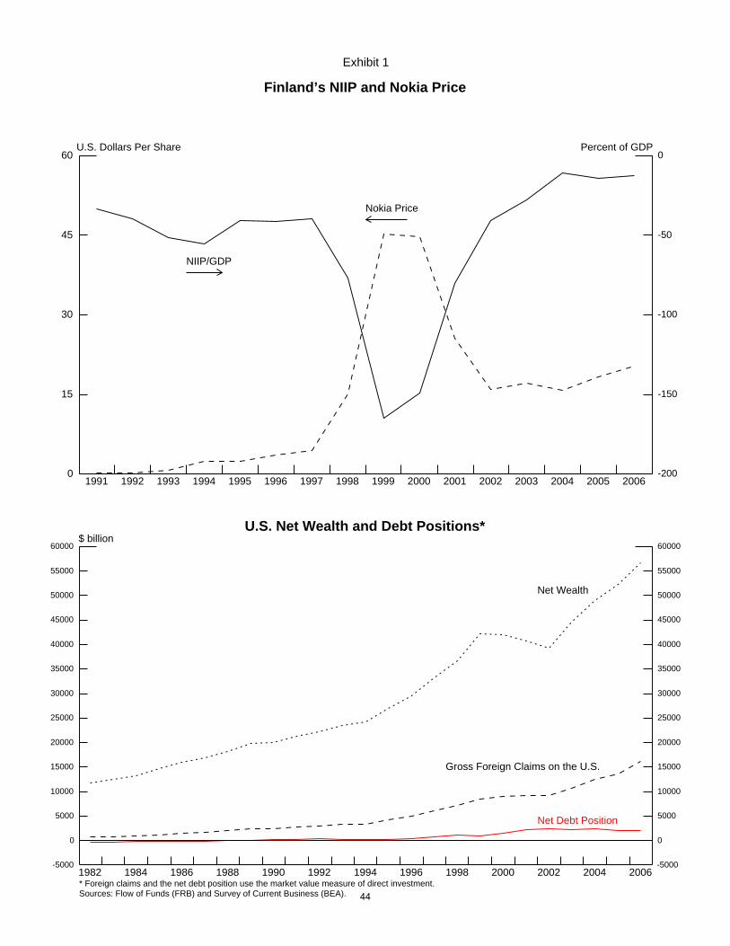
Exhibit 1

Finland’s NIIP and Nokia Price

1991 1992 1993 1994 1995 1996 1997 1998 1999 2000 2001 2002 2003 2004 2005 20060

15

30

45

60

-200

-150

-100

-50

0

Nokia Price

NIIP/GDP

U.S. Dollars Per Share Percent of GDP

1982 1984 1986 1988 1990 1992 1994 1996 1998 2000 2002 2004 2006-5000

0

5000

10000

15000

20000

25000

30000

35000

40000

45000

50000

55000

60000

-5000

0

5000

10000

15000

20000

25000

30000

35000

40000

45000

50000

55000

60000

* Foreign claims and the net debt position use the market value measure of direct investment.Sources: Flow of Funds (FRB) and Survey of Current Business (BEA).

Net Wealth

Gross Foreign Claims on the U.S.

Net Debt Position

U.S. Net Wealth and Debt Positions* $ billion

44

Exhibit 2 04-22-08

Extended Baseline Projection

80

90

100

110

120

2000 2010 2020

Real Exchange RateIndex, 2000q1 = 100

0

1

2

3

4

5

6

2000 2010 2020

Foreign GDP (with US GDP, dashed)4-quarter percent change

0

10

20

30

40

50

60

70

80

90

2000 2010 2020

Oil Import Pricedollars per barrel

0

1

2

3

4

5

6

7

2000 2010 2020

Short-TermLong-Term

US Short & Long-Term Interest Ratespercentage points

0

2

4

6

8

10

2000 2010 2020

Net PositionGovernment PaymentsPrivate PaymentsPrivate Receipts

Rate of Return on Portfolio Investmentpercent, a.r.

-3

0

3

6

9

12

15

2000 2010 2020

ReceiptsPayments

Rate of Return on Direct Investmentpercent, a.r.

45

Exhibit 2 (continued) 04-22-08

Extended Baseline Projection

-15

-10

-5

0

5

10

15

2000 2010 2020

Real Exports4-quarter percent change

-15

-10

-5

0

5

10

15

2000 2010 2020

Real Imports4-quarter percent change

-8

-7

-6

-5

-4

-3

-2

-1

0

2000 2010 2020

Nominal Trade Balance (Ex. Oil, dashed)percent of GDP

-8

-7

-6

-5

-4

-3

-2

-1

0

2000 2010 2020

Current Account Balancepercent of GDP

-80

-70

-60

-50

-40

-30

-20

-10

0

2000 2010 2020

Net International Investment Position/GDPpercent of GDP

-1.00

-0.75

-0.50

-0.25

0.00

0.25

0.50

0.75

1.00

2000 2010 2020

Net Investment Incomepercent of GDP

46

Exhibit 2 (continued further) 04-22-08

Extended Baseline Projection

0

20

40

60

80

100

120

140

160

180

200

1980 1990 2000 2010 2020

Direct Investment ClaimsDirect Investment LiabilitiesPortfolio ClaimsPortfolio Liabilities

Gross Investment Positionspercent of GDP

-2

0

2

4

6

8

10

12

14

16

1980 1990 2000 2010 2020

Rates of Returnpercent

47

Exhibit 3 04-22-08

Alternative Projections

70

80

90

100

110

120

2000 2010 2020

Black: Baseline Green: U.S. Growth = Foreign Growth Red: Oil Prices RiseBlue: Dollar Depreciation and Higher Interest Rates Magenta: Higher Foreign Growth

Real Exchange RateIndex, 2000q1 = 100

0

1

2

3

4

5

6

2000 2010 2020

Foreign GDP (with US GDP, dashed)4-quarter percent change

0

20

40

60

80

100

120

140

160

2000 2010 2020

Oil Import Pricedollars per barrel

0

1

2

3

4

5

6

7

2000 2010 2020

Short-TermLong-Term

US Short & Long-Term Interest Ratespercentage points

0

1

2

3

4

5

6

7

8

2000 2010 2020

Rate of Return on Overall Portfolio Investmentpercent, a.r.

-3

0

3

6

9

12

15

2000 2010 2020

Receipts (Solid)Payments (Dashed)

Rate of Return on Direct Investmentpercent, a.r.

48

Exhibit 3 (continued) 04-22-08

Alternative Projections

-15

-10

-5

0

5

10

15

2000 2010 2020

Black: Baseline Green: U.S. Growth = Foreign Growth Red: Oil Prices RiseBlue: Dollar Depreciation and Higher Interest Rates Magenta: Higher Foreign Growth

Real Exports4-quarter percent change

-15

-10

-5

0

5

10

15

2000 2010 2020

Real Imports4-quarter percent change

-10

-8

-6

-4

-2

0

2000 2010 2020

Nominal Trade Balance (Ex. Oil, dashed)percent of GDP

-10

-8

-6

-4

-2

0

2000 2010 2020

Current Account Balancepercent of GDP

-80

-60

-40

-20

0

2000 2010 2020

Net International Investment Position/GDPpercent of GDP

-1.5

-1.0

-0.5

0.0

0.5

1.0

1.5

2000 2010 2020

Net Investment Incomepercent of GDP

49

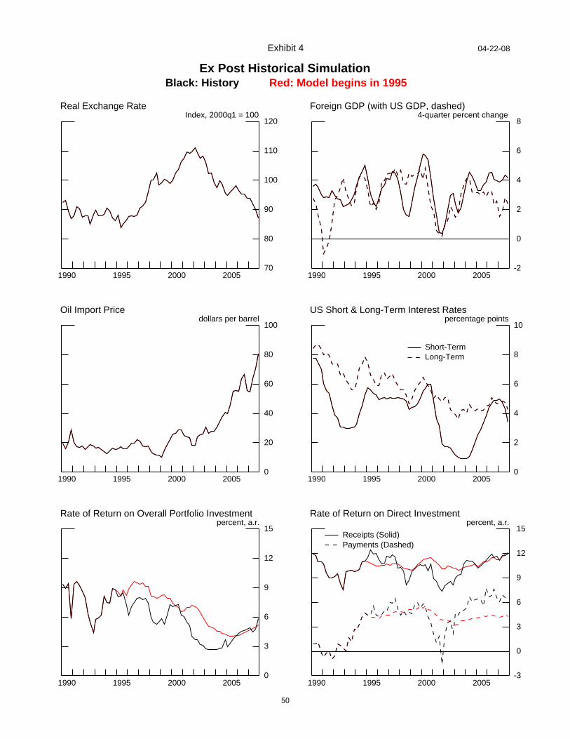
Exhibit 4 04-22-08

Ex Post Historical Simulation

70

80

90

100

110

120

1990 1995 2000 2005

Black: History Red: Model begins in 1995

Real Exchange RateIndex, 2000q1 = 100

-2

0

2

4

6

8

1990 1995 2000 2005

Foreign GDP (with US GDP, dashed)4-quarter percent change

0

20

40

60

80

100

1990 1995 2000 2005

Oil Import Pricedollars per barrel

0

2

4

6

8

10

1990 1995 2000 2005

Short-TermLong-Term

US Short & Long-Term Interest Ratespercentage points

0

3

6

9

12

15

1990 1995 2000 2005

Rate of Return on Overall Portfolio Investmentpercent, a.r.

-3

0

3

6

9

12

15

1990 1995 2000 2005

Receipts (Solid)Payments (Dashed)

Rate of Return on Direct Investmentpercent, a.r.

50

Exhibit 4 (continued) 04-22-08

Ex Post Historical Simulation

-15

-10

-5

0

5

10

15

1990 1995 2000 2005

Black: History Red: Model begins in 1995

Real Exports4-quarter percent change

-15

-10

-5

0

5

10

15

1990 1995 2000 2005

Real Imports4-quarter percent change

-8

-6

-4

-2

0

2

1990 1995 2000 2005

Nominal Trade Balance (Ex. Oil, dashed)percent of GDP

-8

-6

-4

-2

0

2

1990 1995 2000 2005

Current Account Balancepercent of GDP

-30

-25

-20

-15

-10

-5

0

1990 1995 2000 2005

Net International Investment Position/GDPpercent of GDP

-0.25

0.00

0.25

0.50

0.75

1.00

1990 1995 2000 2005

Net Investment Incomepercent of GDP

51

Exhibit 5

-100

-80

-60

-40

-20

0

20

40

60

80

100

120

140

160

NZ Gre Por Aus Spa U.K. Swe Aut U.S. Fin Can Ire Ita Net Fra Ger Bel Jap Swi

Source: IMF International Financial Statistics. Sweden data from 2005.

Net International Investment Position as a Share of GDP, 2006Percent of GDP

-20

-15

-10

-5

0

5

10

15

Ire NZ Aus Por Gre Spa Aut Ita Can Fin U.S. Swe Nor Bel Fra Ger Den U.K. Jap Net Swi

Source: IMF Balance of Payments Statistics.

Net Investment Income as a Share of GDP, 2006Percent of GDP

52

Exhibit 5a

-500

-450

-400

-350

-300

-250

-200

-150

-100

-50

0

50

100

150

200

250

300

Gre NZ Aus Por Spa U.S. U.K. Swe Aut Fin Ita Can Ire Net Fra Bel Ger Swi Jap

Source: IMF International Financial Statistics. Sweden data from 2005.

Net International Investment Position as a Share of Exports, 2006Percent of Exports

-30

-25

-20

-15

-10

-5

0

5

10

15

20

25

NZ Aus Ire Gre Por Spa Ita Aut Can Fin Swe Bel Nor Ger Den Fra U.S. Net U.K. Jap Swi

Source: IMF Balance of Payments Statistics.

Net Investment Income as a Share of Exports, 2006Percent of Exports

53

Exhibit 6

-100 -80 -60 -40 -20 0 20 40 60 80 100 120 140 160-20

-15

-10

-5

0

5

10

15

-20

-15

-10

-5

0

5

10

15

NZ

Gre PorAus

Spa

U.K.

Swe

Aut

U.S.Fin

Can

Ire

Ita

Net

Fra Ger Bel

Jap

Swi

Net International Investment Position / GDP

Net Investment Income / GDPNIIP/GDP vs Net Investment Income/GDP, 2006

54

Exhibit 7

-50

-40

-30

-20

-10

0

10

20

Net International Investment Position as a Share of GDP(Measured at Year of Current Account Adjustment)

Fin Aus Can Can Swe Swe Aut Spa Nor Aut Ita Spa U.S. Ita UK1991 1989 1993 1981 1992 1982 1999 1991 1986 1980 1992 1981 1987 1981 1989

Source: IMF International Financial Statistics.

Percent of GDP

-12

-10

-8

-6

-4

-2

0

2

Net Investment Income as a Share of GDP(Measured at Year of Current Account Adjustment)

NZ Por Ire Can Den Fin Swe Can Aus Gre Gre Ita Swe Aut Nor Spa Spa Ita Aut UK Fra U.S.1984 1982 1981 1981 1986 1991 1992 1993 1989 1985 1990 1992 1982 1999 1986 1981 1991 1981 1980 1989 1982 1987

Source: IMF Balance of Payments Statistics.

Percent of GDP

55

Exhibit 7a

-50

-40

-30

-20

-10

0

10

20

Net International Investment Position as a Share of GDP

Fin Aus Can Can Swe Swe Aut Spa Nor Aut Ita Spa U.S. Ita UK1991 1989 1993 1981 1992 1982 1999 1991 1986 1980 1992 1981 1987 1981 1989

Source: IMF International Financial Statistics.

Measured at Year of Current Account AdjustmentAverage Over Available History Up to Year of Current Account Adjustment

Percent of GDP

-12

-10

-8

-6

-4

-2

0

2

Net Investment Income as a Share of GDP

NZ Por Ire Can Den Fin Swe Can Aus Gre Gre Ita Swe Aut Nor Spa Spa Ita Aut UK Fra U.S.1984 1982 1981 1981 1986 1991 1992 1993 1989 1985 1990 1992 1982 1999 1986 1981 1991 1981 1980 1989 1982 1987

Source: IMF Balance of Payments Statistics.

Measured at Year of Current Account AdjustmentAverage Over Available History Up to Year of Current Account Adjustment

Percent of GDP

56

Exhibit 8

Shares in World Market Capitalization

1993 1994 1995 1996 1997 1998 1999 2000 2001 2002 2003 2004 2005 200630

35

40

45

50

55

Source: S&P’s Global Markets Factbook 2004.

Share of U.S. EquitiesPercent

1994 1995 1996 1997 1998 1999 2000 2001 2002 2003 2004 2005 200630

35

40

45

50

55

Source: BIS data, adjusted for Brady bonds outstanding.

Share of U.S. BondsPercent

57

Exhibit 9

0

5

10

15

20

25

30

35

1997 2001 2002 2003 2004 2005 2006

U.S. equitiesAll external equities

Share of U.S. and All External Equities in Total Equity Portfolios of Foreign InvestorsPercent

0

5

10

15

20

25

30

35

1997 2001 2002 2003 2004 2005 2006Authors’ estimates based on IMF Coordinated Portfolio Asset Surveys.

U.S. bondsAll external bonds

Share of U.S. and All External Bonds in Total Bond Portfolios of Foreign InvestorsPercent

58

Exhibit 10

Share of U.S. Securities in Foreign Investors’ Portfolios of External Securities

0

5

10

15

20

25

30

35

40

45

1997 2001 2002 2003 2004 2005 2006Authors’ estimates based on IMF Coordinated Portfolio Asset Surveys.

EquitiesBonds

Percent

59

Exhibit 11

0.10 0.12 0.14 0.16 0.18 0.20 0.22 0.24 0.26 0.28 0.30 0.32 0.34 0.36 0.380.10

0.12

0.14

0.16

0.18

0.20

0.22

0.24

0.26

0.28

0.30

0.32

0.34

0.36

0.38

1997

2001

2002

2003 2004

20052006

Relative Portfolio Weight in External Equities

Relative Portfolio Weight in U.S. EquitiesForeigners’ Relative Portfolio Weights in U.S. and All External Equities

0.10 0.12 0.14 0.16 0.18 0.20 0.22 0.24 0.26 0.28 0.30 0.32 0.34 0.36 0.380.10

0.12

0.14

0.16

0.18

0.20

0.22

0.24

0.26

0.28

0.30

0.32

0.34

0.36

0.38

1997

20012002

2003

2004

2005

2006

Relative Portfolio Weight in External Bonds

Relative Portfolio Weight in U.S. BondsForeigners’ Relative Portfolio Weights in U.S. and All External Bonds

60

Exhibit 12

Projections of Foreign Holdings of U.S. Securities

0.30

0.32

0.34

0.36

0.38

2004 2006 2008 2010 2012 2014 2016 2018 2020

BaselineAlternative

A. U.S. Market CapitalizationShare of World Market Cap

0.15

0.17

0.19

0.21

0.23

0.25

0.27

0.29

0.31

0.33

0.35

0.37

0.39

0.41

0.43

0.45

0.47

0.49

2004 2006 2008 2010 2012 2014 2016 2018 2020

BaselineAlternative

B. Foreign HoldingsShare of U.S. Market Cap

0.10

0.12

0.14

0.16

0.18

0.20

0.22

0.24

2004 2006 2008 2010 2012 2014 2016 2018 2020

BaselineAlternative

C. U.S. SecuritiesShare of Total Foreign Portfolio

0.25

0.30

0.35

0.40

0.45

0.50

0.55

2004 2006 2008 2010 2012 2014 2016 2018 2020

BaselineAlternative

D. U.S. SecuritiesRelative Weight in Foreign Portfolio

61

(1) (2) (3)† (4)† (5) (6)‡ (7)‡ (8)‡ (9)‡ (10)‡

10-yr. Int. Rate (-1) 0.426 0.578 0.587 0.564 0.559 0.596 0.395 0.596 0.371 0.573SE 0.041 0.059 0.058 0.060 0.062 0.064 0.048 0.063 0.047 0.066t-stat 10.32 9.89 10.09 9.36 9.06 9.37 8.20 9.47 7.87 8.74

10-yr. Int. Rate (-2) 0.157 0.064 0.056 0.057 0.060 0.069 0.176 0.071 0.167 0.060SE 0.028 0.062 0.064 0.056 0.055 0.068 0.031 0.060 0.037 0.062t-stat 5.69 1.03 0.87 1.02 1.10 1.01 5.67 1.17 4.50 0.97

Money Market Int. Rate 0.246 0.198 0.194 0.204 0.211 0.195 0.238 0.170 0.265 0.206SE 0.025 0.030 0.029 0.033 0.036 0.032 0.024 0.033 0.025 0.036t-stat 9.82 6.64 6.82 6.12 5.87 6.12 9.90 5.19 10.72 5.69

Inflation 0.212 0.180 0.185 0.206 0.201 0.177 0.240 0.208 0.246 0.205SE 0.042 0.066 0.065 0.063 0.067 0.066 0.038 0.062 0.044 0.064t-stat 5.08 2.73 2.85 3.25 3.01 2.67 6.36 3.36 5.63 3.18

Real GDP Growth 0.077 0.060 0.064 0.071 0.066 0.049 0.089 0.045 0.110 0.057SE 0.027 0.024 0.026 0.026 0.026 0.026 0.033 0.025 0.040 0.029t-stat 2.88 2.54 2.47 2.72 2.49 1.89 2.72 1.78 2.76 1.94

Int. Rate Volatility 0.093 -0.486 -0.422 -0.392 -0.484 -0.483 0.166 -0.393 0.175 -0.436SE 0.408 0.289 0.288 0.308 0.296 0.324 0.480 0.326 0.526 0.319t-stat 0.23 -1.68 -1.47 -1.27 -1.64 -1.49 0.35 -1.21 0.33 -1.37

Fiscal Balance / GDP -0.005 -0.025 -0.031 -0.022 -0.019 -0.025 -0.004 0.001 -0.035 -0.026SE 0.016 0.011 0.012 0.010 0.011 0.011 0.015 0.012 0.016 0.012t-stat -0.34 -2.17 -2.61 -2.14 -1.71 -2.25 -0.25 0.09 -2.13 -2.23

NIIP / GDP (-1) -0.002 -0.001 -0.001 -0.005 -0.004SE 0.002 0.001 0.001 0.003 0.002t-stat -1.60 -1.25 -2.25 -1.90 -1.92

NIINCOME / GDP (-1) -0.020 0.052 0.030 0.001 -0.016SE 0.059 0.013 0.009 0.103 0.066t-stat -0.35 4.01 3.46 0.01 -0.25

CAB / GDP (-1) 0.008 -0.011 -0.001 -0.003 0.015SE 0.012 0.009 0.008 0.015 0.010t-stat 0.61 -1.21 -0.17 -0.22 1.49

Ext. Liab. Variable (-1) 0.020 -0.004 -0.001 0.006 0.013SE 0.015 0.003 0.002 0.029 0.017t-stat 1.38 -1.43 -0.41 0.19 0.75

Euro -0.072 -0.108 -0.119 -0.055 -0.125 0.000 -0.071 -0.061 -0.197SE 0.137 0.128 0.154 0.120 0.145 0.081 0.090 0.146 0.163t-stat -0.53 -0.84 -0.77 -0.46 -0.86 0.00 -0.79 -0.42 -1.21

Constant 0.267 -0.332 -0.481 -0.113 -0.025 -0.455 0.307 -0.143 -0.020 -0.266SE 0.130 1.058 1.064 0.952 0.937 1.028 0.150 0.711 0.433 0.916t-stat 2.05 -0.31 -0.45 -0.12 -0.03 -0.44 2.05 -0.20 -0.05 -0.29

Time Fixed Effects No Yes Yes Yes Yes Yes No Yes No YesCountry Fixed Effects No Yes Yes Yes Yes Yes No No Yes Yes

R^2 0.938 0.967 0.969 0.970 0.968 0.970 0.945 0.969 0.948 0.970SER 1.060 0.810 0.796 0.787 0.814 0.791 1.022 0.798 1.020 0.798# Observations 541 541 532 518 511 474 438 438 438 438

Except as noted, countries included are Australia, Austria, Belgium, Canada, Denmark, Finland, France, Germany, Greece, Iceland, Ireland, Italy, Japan, Netherlands, New Zealand, Norway, Portugal, Spain, Sweden, Switzerland, the United Kingdom, and the United States.† Excludes Iceland.‡ Excludes Canada, Iceland, and Italy.

Table 1: Panel Regressions for Interest Rates

Dependent Variable: 10-yr Nominal Government Bond Yields

62

(1) (2) (3)† (4)† (5) (6)‡ (7)‡ (8)‡ (9)‡ (10)‡

REER Pct. Dev. (-1) 1.066 1.053 1.066 1.078 1.043 1.046 1.087 1.097 1.021 1.026SE 0.035 0.035 0.031 0.039 0.036 0.026 0.044 0.037 0.044 0.032t-stat 30.32 30.29 34.81 27.90 28.75 40.73 24.86 29.84 23.40 32.09

REER Pct. Dev. (-2) -0.333 -0.321 -0.331 -0.330 -0.313 -0.317 -0.334 -0.327 -0.326 -0.311SE 0.036 0.034 0.031 0.037 0.038 0.035 0.047 0.039 0.054 0.045t-stat -9.27 -9.37 -10.55 -8.83 -8.27 -9.13 -7.06 -8.29 -6.05 -6.91

Money Market Int. Rate 0.178 0.365 0.380 0.363 0.371 0.421 0.198 0.370 0.254 0.417SE 0.081 0.162 0.167 0.169 0.159 0.178 0.090 0.145 0.093 0.170t-stat 2.19 2.25 2.28 2.16 2.33 2.37 2.20 2.56 2.72 2.45

Inflation -0.242 -0.453 -0.427 -0.359 -0.471 -0.440 -0.230 -0.308 -0.334 -0.426SE 0.051 0.136 0.131 0.150 0.146 0.131 0.086 0.131 0.098 0.143t-stat -4.71 -3.33 -3.27 -2.40 -3.23 -3.36 -2.68 -2.34 -3.42 -2.97

Real GDP Growth -0.173 -0.332 -0.344 -0.332 -0.337 -0.274 -0.111 -0.157 -0.167 -0.234SE 0.142 0.173 0.192 0.193 0.198 0.202 0.185 0.190 0.197 0.214t-stat -1.22 -1.92 -1.80 -1.72 -1.70 -1.36 -0.60 -0.83 -0.85 -1.09

Int. Rate Volatility -0.458 -0.937 -0.961 -0.557 -0.871 -1.314 -0.339 -0.244 -0.329 -0.692SE 0.559 1.093 1.146 1.225 1.022 1.226 0.549 0.944 0.821 1.202t-stat -0.82 -0.86 -0.84 -0.45 -0.85 -1.07 -0.62 -0.26 -0.40 -0.58

Fiscal Balance / GDP 0.014 0.094 0.116 0.073 0.030 0.185 0.072 0.118 0.048 0.125SE 0.050 0.108 0.107 0.107 0.097 0.118 0.067 0.061 0.113 0.127t-stat 0.28 0.87 1.09 0.68 0.31 1.57 1.07 1.93 0.43 0.98

NIIP / GDP (-1) 0.016 0.013 0.017 0.011 0.013SE 0.009 0.007 0.007 0.014 0.014t-stat 1.76 1.81 2.66 0.78 0.96

NIINCOME / GDP (-1) 0.356 -0.052 -0.067 0.552 0.486SE 0.200 0.083 0.087 0.275 0.261t-stat 1.78 -0.62 -0.76 2.01 1.86

CAB / GDP (-1) -0.002 -0.068 -0.077 -0.191 -0.166SE 0.103 0.080 0.092 0.115 0.138t-stat -0.02 -0.86 -0.84 -1.66 -1.20

Ext. Liab. Variable (-1) 0.271 0.001 0.012 0.509 0.486SE 0.129 0.021 0.023 0.233 0.251t-stat 2.10 0.05 0.52 2.19 1.93

Euro 0.099 0.362 0.524 0.148 -0.486 0.632 0.294 -0.095 -0.138SE 0.837 0.858 0.897 0.849 1.106 0.657 0.759 0.946 1.283t-stat 0.12 0.42 0.58 0.17 -0.44 0.96 0.39 -0.10 -0.11

Constant 0.677 -0.598 -0.513 -0.755 -0.344 -2.039 0.310 -1.746 -0.668 -2.507SE 0.673 2.090 2.146 2.377 2.268 2.452 0.754 1.218 1.426 2.664t-stat 1.01 -0.29 -0.24 -0.32 -0.15 -0.83 0.41 -1.43 -0.47 -0.94

Time Fixed Effects No Yes Yes Yes Yes Yes No Yes No YesCountry Fixed Effects No Yes Yes Yes Yes Yes No No Yes Yes

R^2 0.7116 0.7705 0.7749 0.7864 0.7701 0.7741 0.7301 0.7771 0.7463 0.7901SER 5.0163 4.7281 4.6858 4.5901 4.8073 4.6942 4.9430 4.6687 4.9065 4.6473# Observations 497 497 488 480 473 434 404 404 404 404

Except as noted, countries included are Australia, Austria, Belgium, Canada, Denmark, Finland, France, Germany, Greece, Iceland, Ireland, Italy, Japan, Netherlands, New Zealand, Norway, Portugal, Spain, Sweden, Switzerland, the United Kingdom, and the United States.† Excludes Iceland.‡ Excludes Canada, Iceland, and Italy.

Dependent Variable: Real Effective Exchange Rate as Percent Deviation from Sample Mean

Table 2: Panel Regressions for Exchange Rates

(Note: Means calculated by country.)(Note: REER is home relative to foreign. An increase is an appreciation.)

63

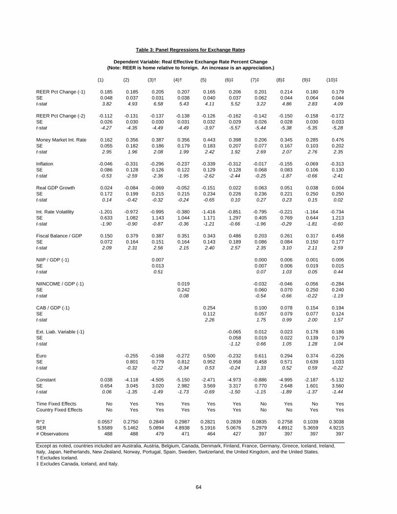
(1) (2) (3)† (4)† (5) (6)‡ (7)‡ (8)‡ (9)‡ (10)‡

REER Pct Change (-1) 0.185 0.185 0.205 0.207 0.165 0.206 0.201 0.214 0.180 0.179SE 0.048 0.037 0.031 0.038 0.040 0.037 0.062 0.044 0.064 0.044t-stat 3.82 4.93 6.58 5.43 4.11 5.52 3.22 4.86 2.83 4.09

REER Pct Change (-2) -0.112 -0.131 -0.137 -0.138 -0.126 -0.162 -0.142 -0.150 -0.158 -0.172SE 0.026 0.030 0.030 0.031 0.032 0.029 0.026 0.028 0.030 0.033t-stat -4.27 -4.35 -4.49 -4.49 -3.97 -5.57 -5.44 -5.38 -5.35 -5.28

Money Market Int. Rate 0.162 0.356 0.387 0.356 0.443 0.398 0.206 0.345 0.285 0.476SE 0.055 0.182 0.186 0.179 0.183 0.207 0.077 0.167 0.103 0.202t-stat 2.95 1.96 2.08 1.99 2.42 1.92 2.69 2.07 2.76 2.35

Inflation -0.046 -0.331 -0.296 -0.237 -0.339 -0.312 -0.017 -0.155 -0.069 -0.313SE 0.086 0.128 0.126 0.122 0.129 0.128 0.068 0.083 0.106 0.130t-stat -0.53 -2.59 -2.36 -1.95 -2.62 -2.44 -0.25 -1.87 -0.66 -2.41

Real GDP Growth 0.024 -0.084 -0.069 -0.052 -0.151 0.022 0.063 0.051 0.038 0.004SE 0.172 0.199 0.215 0.215 0.234 0.226 0.236 0.221 0.250 0.250t-stat 0.14 -0.42 -0.32 -0.24 -0.65 0.10 0.27 0.23 0.15 0.02

Int. Rate Volatility -1.201 -0.972 -0.995 -0.380 -1.416 -0.851 -0.795 -0.221 -1.164 -0.734SE 0.633 1.082 1.143 1.044 1.171 1.297 0.405 0.769 0.644 1.213t-stat -1.90 -0.90 -0.87 -0.36 -1.21 -0.66 -1.96 -0.29 -1.81 -0.60

Fiscal Balance / GDP 0.150 0.379 0.387 0.351 0.343 0.486 0.203 0.261 0.317 0.458SE 0.072 0.164 0.151 0.164 0.143 0.189 0.086 0.084 0.150 0.177t-stat 2.09 2.31 2.56 2.15 2.40 2.57 2.35 3.10 2.11 2.59

NIIP / GDP (-1) 0.007 0.000 0.006 0.001 0.006SE 0.013 0.007 0.006 0.019 0.015t-stat 0.51 0.07 1.03 0.05 0.44

NIINCOME / GDP (-1) 0.019 -0.032 -0.046 -0.056 -0.284SE 0.242 0.060 0.070 0.250 0.240t-stat 0.08 -0.54 -0.66 -0.22 -1.19

CAB / GDP (-1) 0.254 0.100 0.078 0.154 0.194SE 0.112 0.057 0.079 0.077 0.124t-stat 2.26 1.75 0.99 2.00 1.57

Ext. Liab. Variable (-1) -0.065 0.012 0.023 0.178 0.186SE 0.058 0.019 0.022 0.139 0.179t-stat -1.12 0.66 1.05 1.28 1.04

Euro -0.255 -0.168 -0.272 0.500 -0.232 0.611 0.294 0.374 -0.226SE 0.801 0.779 0.812 0.952 0.958 0.458 0.571 0.639 1.033t-stat -0.32 -0.22 -0.34 0.53 -0.24 1.33 0.52 0.59 -0.22

Constant 0.038 -4.118 -4.505 -5.150 -2.471 -4.973 -0.886 -4.995 -2.187 -5.132SE 0.654 3.045 3.020 2.982 3.569 3.317 0.770 2.648 1.601 3.560t-stat 0.06 -1.35 -1.49 -1.73 -0.69 -1.50 -1.15 -1.89 -1.37 -1.44

Time Fixed Effects No Yes Yes Yes Yes Yes No Yes No YesCountry Fixed Effects No Yes Yes Yes Yes Yes No No Yes Yes

R^2 0.0557 0.2750 0.2849 0.2987 0.2821 0.2839 0.0835 0.2758 0.1039 0.3038SER 5.5589 5.1462 5.0894 4.8938 5.1916 5.0676 5.2979 4.8912 5.3659 4.9215# Observations 488 488 479 471 464 427 397 397 397 397

Except as noted, countries included are Australia, Austria, Belgium, Canada, Denmark, Finland, France, Germany, Greece, Iceland, Ireland, Italy, Japan, Netherlands, New Zealand, Norway, Portugal, Spain, Sweden, Switzerland, the United Kingdom, and the United States.† Excludes Iceland.‡ Excludes Canada, Iceland, and Italy.

Table 3: Panel Regressions for Exchange Rates

Dependent Variable: Real Effective Exchange Rate Percent Change(Note: REER is home relative to foreign. An increase is an appreciation.)

64

Table 4: Standard Determinants of Current Account / GDP

1 2 3 4Per Capita GDP 0.003 0.005 0.010 0.011

3.200 3.806 4.475 4.628ΔGrowth 0.032 0.066 ‐0.063 ‐0.010

0.396 1.043 ‐0.436 ‐0.102Fiscal Balance 0.189 0.185 0.214 0.207

2.864 3.333 2.616 3.063NFA 0.018 0.016 0.013 0.011

2.765 2.603 2.526 2.713Age Dependency Ratio -0.025 ‐0.010 -0.068 -0.041

‐1.954 ‐0.574 ‐3.233 ‐1.627Oil Balance / GDP 0.158 0.156 0.165 0.168

3.130 3.038 2.452 2.367Openness 0.012 0.006 0.010 0.000

1.996 1.099 1.012 0.064Governance Indicators -0.018 -0.015

‐2.379 ‐2.133U.S.(1997 ‐ 2006) -0.060 -0.077

‐3.752 ‐4.174Developing Asia (1997‐2006) 0.047 0.047

4.666 8.520

#Obs 346 346 221 221R^2 0.313 0.364 0.372 0.445SER 0.035 0.034 0.037 0.034

Panel regression with unreported constant and period fixed effects.  84 cross‐sections and 5 periods.t-statistic reported underneath coefficientBold indicates signifance at the 10 percent level.Developing Asia includes China, Hong Kong, Indonesia, Korea, Malaysia,      Philippines, Taiwan, and Thailand

65