Embed Size (px)
Citation preview
How much for a haircut?
Illiquidity, secondary markets, and the value of private equity
Nicolas P.B. Bollen* Vanderbilt University
Berk A. Sensoy Ohio State University
April 24, 2015
Abstract
Limited partners (LPs) of private equity funds commit to invest with significant
uncertainty regarding the timing of capital calls and payoffs and extreme
restrictions on liquidity. Secondary markets have emerged which alleviate some of
the associated cost. This paper develops a subjective valuation model that
incorporates these institutional features. For a risk-averse LP private equity values
are highly sensitive to the time-varying discount observed in secondary market
transactions. Model-implied breakeven returns generally exceed empirically
observed returns. Only for highly risk-tolerant LPs who can access above-average
funds and an efficient secondary market are the costs of private equity justified by
performance.
Preliminary; please do not circulate
*Corresponding author. Contact information: Nicolas P.B. Bollen, The Owen Graduate School of Management,
Vanderbilt University, 401 21st Avenue South, Nashville, TN 37203, Telephone: 615-343-5029, Email:
[email protected]. Berk A. Sensoy, Department of Finance, Fisher College of Business, Ohio State
University, Columbus, OH 43210, Telephone: 614-292-3217, email: [email protected]. For helpful comments and
discussions, we thank Nick Crain and seminar participants at Boston College, University of Michigan, University of
Utah, and Vanderbilt University. This research is supported by the Financial Markets Research Center at Vanderbilt
University and The Risk Institute at the Fisher College of Business, Ohio State University.
1
Introduction
Institutional investors now routinely allocate 15% to 30% of their portfolios to private equity
funds. This capital is committed with extreme restrictions on liquidity. Private equity funds are
organized as 10 to 12 year partnerships, with investors as limited partners (LPs) and the fund
manager as the general partner (GP). Importantly, during the partnership’s life there is no option
to redeem a stake with the fund. Instead, LPs requiring an early exit from the partnership must turn
to the secondary market to sell their stakes, usually at a substantial discount from fund NAV. These
haircuts can reach fire sale levels in times of broader market dislocations, such as during the recent
global financial crisis. Moreover, even while invested in the fund, LPs face a large degree of
uncertainty regarding the timing and magnitude of capital calls for investments in portfolio
companies and payoffs from exited portfolio companies. These liquidity arrangements intuitively
affect the ex-ante value of commitments to private equity funds. Despite the importance of private
equity to institutional portfolios, to date no academic research provides adequate guidance
regarding the impact of the LP’s illiquidity on their required rate of return.
In this paper, we develop a valuation model for commitments to private equity funds from
the perspective of a risk-averse LP subject to liquidity shocks, such as those brought on by the
crisis, which force the LP to seek an early exit from the partnership. In the model, the market is
incomplete and private equity cannot be fully spanned by public equity, so present values are not
well-defined and an LP’s subjective valuation is relevant. The model explicitly incorporates both
the secondary market, which we assume the LP accesses when a liquidity shock occurs, and
uncertainty about the timing of capital calls and distributions. We show that each of these features
has a quantitatively important impact on the value of commitments to private equity funds.
The model allows us to evaluate several closely related questions that are central to
assessing any alternative asset class. How large are the returns required to compensate for the
special liquidity risks borne by LPs, and how do these compare to actual returns to private equity
funds in the data? How do required returns depend on an LP’s tolerance for risk, the efficiency of
the secondary market, and the fees charged by the GP? What is the impact of diversification across
public and private equity and how does an LP’s allocation to private equity affect the return it
requires? Equivalently, how does an LP’s allocation to private equity depend on the returns it
expects?
2
In the spirit of the real options literature, we model the joint evolution of private and public
equity asset values using a three-dimensional lattice in discrete time. The lattice allows us to
efficiently accommodate a number of path dependencies, including forced secondary sales and
stochastic capital calls and distributions. The lattice is used to compute the certainty equivalent
value of the LP’s portfolio at fund inception using backward recursion, exploiting the fact that
private equity funds have a finite contracted life. In most of our analyses, we solve for the return
and CAPM alpha of the private equity assets (portfolio companies) required to make the LP’s
certainty equivalent equal to the certainty equivalent from a benchmark portfolio consisting only
of public equities and a risk-free bond. From this gross-of-fee breakeven required return on private
equity assets we compute the corresponding net-of-fee LP performance measures commonly used
in the academic literature and in practice: the IRR, TVPI, and PME.1 We illustrate how these
breakeven returns vary with the LP’s risk aversion and allocation to private equity, as well as the
efficiency of the secondary market. We also perform analyses in which we solve for an LP’s
optimal allocation to private equity given a particular expected return on private equity
investments. Naturally, the results depend on the model inputs. We calibrate parameters to the data
wherever possible; individual LPs can use our procedure to generate their own benchmarks.
We begin with the case of an LP portfolio consisting of two assets, a private equity fund
and a risk-free bond. The purpose is to illustrate the impact of the private equity institutional
features novel to our approach in the simplest possible setting. Our first finding is that relative to
a benchmark in which capital calls and distributions occur at known times, uncertain capital calls
and distributions can reduce the LP’s valuation by up to 10% of initial wealth.
Next we introduce liquidity shocks which force an LP to sell its stake on the secondary
market at some discount to NAV. Empirical evidence of secondary markets indicates that the size
of haircuts varies systematically over time, and for this reason we allow for different haircuts in
future secondary market transactions. When haircuts are large, i.e., the secondary market is
inefficient, private equity investments are worth as much as 15% to 25% less than when haircuts
are small, especially to LPs with higher risk aversion. Risk-tolerant LPs are much less sensitive to
1 The TVPI, or total value to paid-in capital, is the undiscounted ratio of the payoffs received by the LP, which come
from distributions to the LP of proceeds from exited or liquidated portfolio companies, to the capital calls paid by the
LP to the fund. The PME, or public market equivalent, is the ratio of discounted distributions to discounted capital
calls, using the realized public market return as the discount rate.
3
the magnitude of secondary market haircuts. Consistent with this, required breakeven private
equity asset returns and net-of-fee LP returns are more highly sensitive to the efficiency of the
secondary market when the LP is more risk averse. The required breakeven returns that emerge
from this analysis far exceed the documented empirical performance of private equity funds,
suggesting that standalone PE investments are unwise for most LPs.
Next, we consider the impact of fees. Again, we solve for breakeven asset returns by setting
the ex-ante value of a portfolio of public equity and a risk-free bond to the value of a portfolio of
private equity and a risk-free bond. We find that moving from a hypothetical zero-fee fund to one
with the typical 2% per year management fee plus 20% carried interest increases the breakeven
private equity asset return by about 20% to 25%. And if fees are doubled, the break-even asset
return increases by another 20% to 25%. Thus, in our model fees to the GP can raise the asset
return required for the LP to breakeven by over 50%.
A more realistic case is one in which the LP holds private equity in a portfolio together
with public equity and a risk-free bond. Here we ask, for a given allocation to private equity, what
private equity returns are required to generate the same certainty equivalent as a portfolio
consisting of 80% public equity and 20% in a risk-free bond.2 Given the diversification benefit
achieved when mixing public and private equity, as well as the smaller allocation to private equity
compared to the prior analysis, we find more modest breakeven asset and fund returns.
Nevertheless, breakeven returns are still greater than empirical estimates of typical fund
performance for most parameter values, indicating that for many LPs the returns they receive in
practice are insufficient to compensate for the risks of private equity. Recent empirical work finds
an average buyout net-of-fee PME of approximately 1.2 to 1.3, indicating 20% to 30%
outperformance relative to the S&P 500 over the life of the fund, and finds that venture capital has
roughly equaled public equities since 2000.3 In our model, these returns are below the LP’s
breakeven return except for risk-tolerant LPs facing an efficient secondary market. That said, those
LPs who are able to access or select above-average funds may find private equity attractive even
at allocations up to 60%.
2 A 10 to 20% allocation to fixed income and cash is typical for endowments and affiliated foundations, according to
the 2014 NACUBO-Commonfund Study of Endowments. Results are similar using instead a benchmark portfolio
consisting of 90% public equity and 10% risk-free bonds. 3 See Harris et al. (2014) for a summary.
4
Our last analysis solves for the optimal allocation to public and private equity in a three-
asset portfolio that includes a risk-free bond. We consider a relatively efficient and a relatively
inefficient secondary market, and vary investor risk aversion. Our results indicate that the
relatively high allocations to private equity made by large endowments (e.g., Yale had a 35%
allocation in 2013) are likely to be optimal to the extent that such institutions are relatively risk
tolerant and able to access or select better funds. However, even then the efficiency of the
secondary market has a substantial impact on the optimal allocation to private equity. When
calibrated to venture capital, for example, the optimal allocation for a risk-tolerant investor is 37%
with an efficient secondary market but only 27% otherwise. For a risk-averse investor, the optimal
allocation drops from a much smaller 11% all the way to 6%.
This paper contributes to several strands of the private equity literature. A key contribution
of this paper is to help interpret empirical work on the performance of private equity funds.
Robinson and Sensoy (2013), Harris, Jenkinson, and Kaplan (2014), Higson and Stucke (2014),
and Phalippou (2013) all use recent data and provide similar estimates of the performance of PE
as an asset class.
Although there is a general consensus on what the performance of private equity funds has
been, there is no clear agreement on whether this performance is sufficient to appropriately
compensate LPs. Our work adds to a nascent literature attempting to shed light on this question.
In an important contribution, Sorensen, Wang, and Yang (2014) develop a method to value private
equity using European option-pricing techniques in continuous time, which requires them to
abstract from the secondary market and stochastic capital calls and distributions. No prior work
incorporates these key institutional features, which are naturally suited to the real-options
framework adopted here and, as we show below, have a quantitatively important impact on the ex-
ante value of private equity commitments. In addition, despite the fact that institutional investors
differ markedly in their allocations to private equity, no prior work examines how breakeven
returns vary with the magnitude of these allocations or provides guidance on optimal allocations.
Our work is also related to recent theoretical work in asset pricing analyzing private equity
performance measures, particularly the PME. Korteweg and Nagel (2013) and Sorensen and
Jagannathan (2013) show that the PME is an appropriate risk-adjusted return for an investor with
log utility if the risk of private equity is spanned by the public market portfolio. In this case, the
5
relevant PME benchmark is one. Our work shows that given the liquidity risks of private equity,
the appropriate PME benchmark is often substantially greater than one, especially for more risk-
averse LPs.
Finally, our work connects to the literature on the fees charged by private equity funds. A
continuing debate is whether fees charged in practice are justified by the returns investors
ultimately receive. Robinson and Sensoy (2013) partially address this question by showing that
higher-fee funds do not earn lower net-of-fee returns. Yet, their analysis speaks only to the cross-
section and not to whether the typical level of fees is excessive. In our model, the answer is
typically yes.
The rest of the paper is organized as follows. In Section I we provide some relevant
institutional detail of private equity funds. Section II explains our procedure for computing an LP’s
subjective valuation of private equity investment. Section III discusses base-case parameter
selection. Main results for portfolios of private equity and risk-free bonds, as well as an allocation
across public equity, private equity, and risk-free bonds, are presented in Section IV. We offer a
summary in Section V.
I. Investments in Private Equity Funds – The Institutional Detail
Private equity funds are generally organized as limited liability partnerships (LLPs) with a
contracted life of ten years. The fund is managed by a private equity firm such as Blackstone,
which serves as the general partner (GP) of the partnership. Investors in the fund, typically large
institutions, are the limited partners (LPs). LPs are passive investors in the fund. At fund inception,
LPs commit to provide capital for management fees and for the fund to make investments in
portfolio companies. These commitments are not transferred to the GP immediately. Instead, the
GP calls capital for investments at its discretion when it identifies investment opportunities.
Similarly, LPs receive cash distributions when the GP chooses to exit portfolio companies through
an IPO, acquisition, or liquidation.
As noted above, LPs typically cannot redeem their stakes with the GP, in contrast to other
forms of delegated asset management such as mutual funds and hedge funds. Liquidity restrictions
on LPs are a consequence of the nature of the underlying portfolio company investments. By
6
definition, private equity securities are those for which there is not an organized exchange, and the
private equity model is to hold investments for a period of years in an effort to add value, typically
through financial or operational engineering. Forced sales of these securities to meet LP
redemption demands would impose large transactions costs on the fund and other LPs as well as
eliminate the opportunity to add value. Moreover, capital calls and distributions are at the GP’s
discretion, and hence stochastic from the LP’s perspective, because presumably the GP has greater
ability than the LP to select and time portfolio company investments and exits. If this were not the
case there would be little reason for an LP to invest in a private equity fund.
In response to the illiquidity of LP stakes, secondary markets have emerged which allow
an LP to sell its stake to other institutions. The efficiency of these markets can be measured by the
discount or haircut a selling LP must accept relative to fair value. Empirical evidence on private
equity secondary transactions is scarce, however Kleymenova et al. (2012) report an average bid
haircut of 25.2% over the 2003-2010 period. They also report considerable countercyclical
variation, with haircuts averaging 8.7% in 2006 and 56.7% in 2009.4
GPs are compensated with a management fee and a share of the profits earned by the fund,
called carried interest. The most common management fee is 2% of committed capital per year, so
that an LP who commits $100 million pays a total of $20 million in management fees over a ten-
year horizon, leaving $80 million for investments in portfolio companies. The most common
carried interest arrangement is 20% of profits, with LPs receiving their committed capital back,
plus a hurdle rate of 8%, before carried interest is earned. Typically, a catch-up provision specifies
that GPs receive 100% of further distributions until they have received 20% of total profits. After
that point, additional proceeds are split between LPs and GPs according to the carried interest rate.
See Gompers and Lerner (1999), Metrick and Yasuda (2010), and Robinson and Sensoy (2013)
for descriptions of different management fee and carried interest arrangements.
There are two main types of private equity funds categorized by the nature of their portfolio
companies. Venture capital funds invest in early stage pre-IPO companies and do not use debt.
Buyout funds, in contrast, invest in more established companies, including public firms, usually
with substantial leverage. Consequently, systematic differences in risk and performance are
4 In practice, discounts are computed treating fund NAVs as fair values despite the fact that they are potentially subject
to manipulation by the GP. Braun et al. (2014), Brown et al. (2014), and Barber and Yasuda (2014) find that NAVs
are generally fair, but are sometimes manipulated when the GP is raising capital for a new fund.
7
typically observed, hence empirical analysis is often undertaken and results reported on venture
capital funds separately from buyout funds. Henceforth when discussing issues that apply to both
we use the general term private equity, as in Section II which presents our valuation model. When
presenting numerical results, as in Section IV, we report two sets of analyses with parameters
selected to represent either venture capital or buyout funds.
II. The Model
Consider a risk averse LP with initial wealth W0 and a CRRA utility function for date T
wealth WT given by
(1)
where measures the LP’s risk aversion.5 The LP can allocate wealth at date 0 across three assets:
a risk-free bond, the public equity market, and a private equity fund managed by a GP. Let x denote
the fraction of initial wealth W0 invested in the private equity fund, y denote the fraction of initial
wealth allocated to the public market, and denote the remaining fraction of initial
wealth invested in a risk-free bond, with . Denote corresponding dollar amounts as
X0, Y0, and Z0, respectively.
II.A. Preliminaries
II.A.1. Private Equity Funds
The private equity fund has a maximum investment life of T, though the GP may sell or
“liquidate” fund assets and distribute proceeds earlier. The LP’s participation in the private equity
fund involves a quantity of capital fixed at date 0, known as committed capital, which is itself split
into two categories. The first is investment capital, denoted by I0, which the LP pays to the GP
once suitable assets are identified and the investment capital is called by the GP. The second are
management fees, which are a fixed percentage m of committed capital and are paid at the end of
every period with the first payment on date 1 and the last payment on the liquidation date. To
simplify analysis of fund performance we collapse this arrangement into a single cash outflow by
5 An alternative specification is the utility of lifetime periodic consumption, for which an investment in private equity
requires a temporary commitment of capital. See Sorensen et al. (2014).
1 1T TU W W
1– –z x y
0 , , 1x y z
8
the LP at date 0 and a single cash inflow on the liquidation date. In particular, we assume that both
investment capital and the present value of management fees for the full horizon T are set aside at
date 0 in an interest bearing account earning the risk-free rate rf. This avoids uncertainty in the
ability of the LP to supply investment capital when called.6 Interest earned on the investment
capital prior to the call date is retained by the LP in the risk-free account. Management fees are
paid at the end of each period out of the account. On the liquidation date, the single cash inflow is
defined as the distribution from the GP and the remaining balance in the risk-free account.
Private equity funds often use leverage to increase the scale of asset purchases. We assume
the GP issues zero-coupon debt in the amount of D0 when investment capital is called and assets
are purchased so that fund assets are initially worth A0 = I0 + D0. The leverage ratio is defined as
D0/I0. We assume that debt is effectively risk free, which can be motivated by buyout firms’
incentives to implicitly guarantee debt with other assets to maintain the ability to borrow in the
future, and hence the yield on fund debt is rf.7
In practice the GP makes multiple capital calls, invests in a portfolio of assets, and
distributes proceeds from asset sales as they occur. Like Sorensen et al. (2014), we assume for
simplicity a single capital call and a single liquidation date, on which proceeds from asset sales
are distributed among debt investors, LPs, and the GP taking into account the seniority of debt
investor claims, a hurdle rate for fund performance, and the carried interest earned by the GP.
However, unlike prior work, we allow both capital calls and distributions to be stochastic. We
denote the share of asset sales flowing to LPs and GPs as and , respectively. See
the Appendix for details on the “waterfall” calculation of these shares.
II.A.2. Joint Evolution of Public and Private Equity
To account for the correlation between the returns of public and private equity, and to allow
for other links between the two markets, we need to model their joint dynamics. We assume that
6 This uncertainty can be important in practice when, for example, and LP makes multiple commitments in anticipation
of a sequence of calls, and the calls instead cluster. 7 In practice the debt is not risk-free and would yield something above the risk-free rate. However, given our
assumptions regarding expected private equity asset expected returns, the probability that bondholders are not repaid
in full has an inconsequential impact on realized bond returns.
tLP A tGP A
9
the returns of public (U) and private (V) equity are governed by a bivariate normal distribution
over each fraction t of a year:
(2)
where and are the annual mean and volatility of returns, respectively, and is the correlation
between public and private equity returns. In some parts of the analysis we consider stand-alone
investments in public or private equity, and in those cases we use the corresponding marginal
distribution. Our focus is on the LP’s ability to exit the private equity fund on a secondary market
prior to the liquidation date, and for this reason our valuation framework employs a discrete-time
numerical technique. Over each period, we allow the value of public and private equity to either
increase, stay the same, or decrease, with probabilities and magnitudes chosen to match the
distributional assumption in (2). In other words, we calibrate a trinomial distribution to match each
assumed normal distribution. Discretizing return distributions in this way is a standard technique
in the literature on valuing payoffs with features resembling American options, which arise here
because of both secondary sales and stochastic capital calls and distributions.
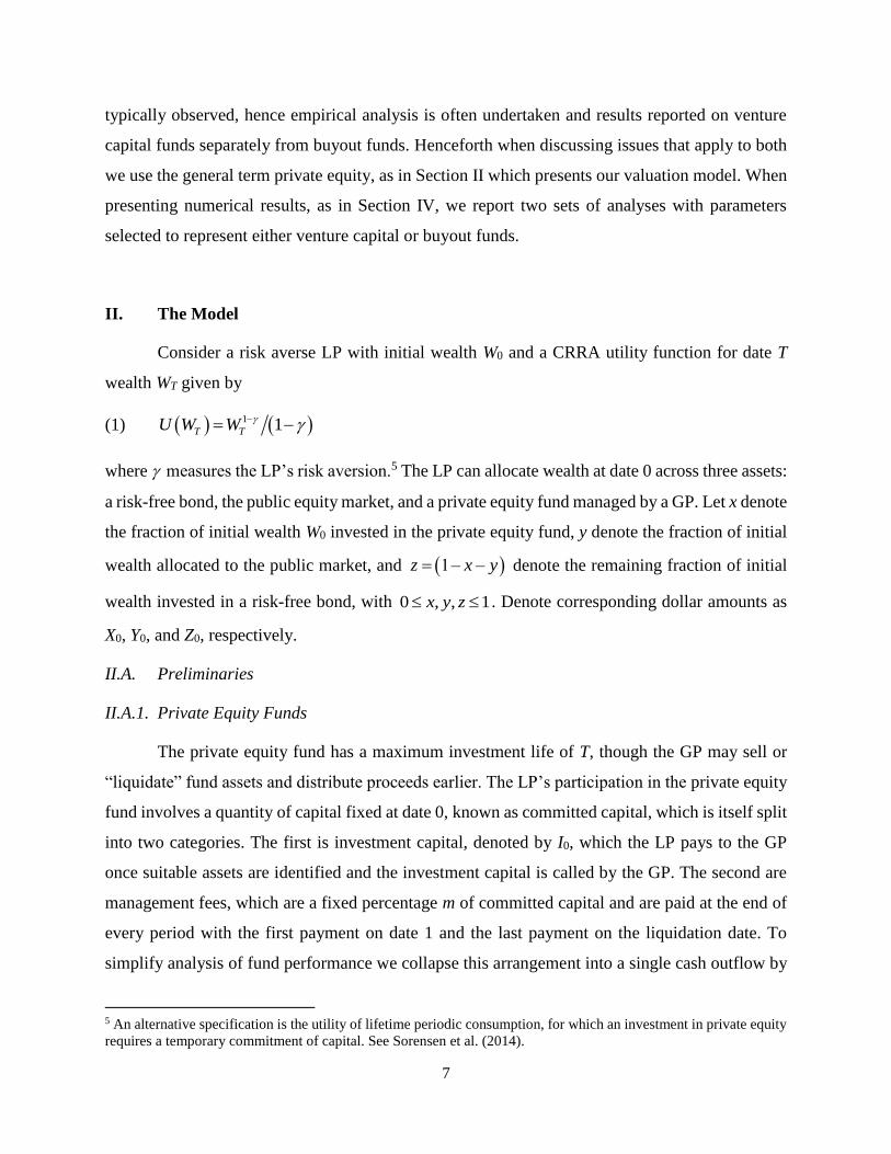
Figure 1 illustrates the possible paths the value of private equity investment capital can
take over the T periods in the life of the fund. Capital committed at date 0 may be called
immediately and invested by the GP, in which case its value will either increase, stay the same, or
decrease each period. If the investment capital is not called its value remains unchanged until the
beginning of the next period. Figure 2 illustrates the possible paths the investment in both public
and private equity can take. Figure 2A describes the three dimensions: time and the values of
public and private equity. We assume that the investment in public equity occurs immediately
upon the allocation decision at date 0. After the capital committed to the private equity fund is
called there are nine joint outcomes possible at each point as shown in Figure 2B. As described in
the Appendix and corresponding Table A1, we determine the nine branch probabilities by
separating the public and private equity value changes. The public equity evolves according to its
marginal distribution, and then the private equity evolves according to its conditional distribution,
where the conditioning information is whether the public equity increased, stayed the same or
decreased. Figure 2C shows this decomposition.
2 2, ~ , , , , ,U V U V U Vr r BVN t t t t
10
We achieve changes in asset values via multiplicative factors. From one date to the next,
the LP’s stake in the public market can increase by a factor eu, decrease by a factor e–u or stay the
same. Once private capital is called and invested by the GP, the value of the purchased assets will
increase by a factor ev, decrease by a factor e–v or stay the same. When analyzing changes in either
public or private markets in isolation, we will need the trinomial probabilities for changes in the
value of the relevant market according to its marginal distribution. For these, we denote the
probabilities of an increase, no change, and a decrease as p1, p0, and p-1, respectively. In general,
we will need the joint probabilities for changes in the values of public and private markets. For
these we denote the probability of an increase in both markets as p1,1, with other branches defined
similarly with the first subscript indicating the change in the public market.
II.A.3. Liquidity Shocks and the Secondary Market
We assume that LPs sell their stakes on the secondary market only in response to a shock
to their liquidity needs. At each point in time, we assume there exists the probability that a
liquidity shock occurs the following period. If a liquidity shock does occur, we assume that the LP
sells all risky assets on the secondary market and invests fully in the risk-free bond, i.e., a flight to
safety.
In addition to forced sales, the model can accommodate voluntary early exercise by which
the LP can decide at each node whether to exercise its real option to transact on the secondary
market or continue to hold the position in the private equity fund for an additional period. Early
exercise may be optimal, for example, when liquidity shocks are somewhat predicable by the LP,
and if haircuts widen substantially when liquidity shocks occur. We find that in our model LP’s
do not generally exercise early unless the probability of a liquidity shock is quite large.
Consequently, for clarity, we omit this possibility in our analyses.
The probability of a liquidity shock is likely related to the performance of risky assets. We
set the probability of a liquidity shock at a given node equal to a base rate of 1% per quarter that
increases by 1% for every net decrease in public equity asset value. We assume that if the LP sells
its stake in the private equity fund in a secondary market the sale will require the LP to accept a
discount or haircut. Empirically, average haircuts vary over time, reflecting the overall appetite for
alternative assets and suggesting that the size of the haircut has a systematic component. One might
imagine an idiosyncratic component as well, if for example counterparties can prey on LPs that
11
have experienced a liquidity shock.8 We could make the size of the haircut a function of asset
values but for simplicity assume that the haircut can take one of two values. The discount then is
a multiplicative factor that is either in a high or low state, HH or HL, where H is a haircut with
0 1H LH H . We denote the probability of each state occurring as pH or pL, which we set as
a non-linear function of cumulative public equity returns, with a larger (smaller) haircut much
more likely when public equity falls (rises) in value. In particular, we set the probability of a large
haircut equal to 0.5 sign i i T where i is the number of net increases, when positive, or
decreases, when negative, in public equity at a particular node. See Figure 3 for an illustration of
these probabilities. With these assumptions, the size of the haircut conditional on a liquidity shock
does not depend on asset values but, because liquidity shocks are more likely when asset values
decline, unconditional expected haircuts are larger when asset values are low.
To operationalize these haircuts, suppose that the LP approaches the secondary market at
some date t after the call date, and fund asset levels are worth At at that time. We assume that the
market price for the LP’s stake in the fund would be a fraction H of the payoff that would accrue
to the LP if the GP were to immediately sell the fund assets, i.e., the LP’s payoff after bondholders
and the GP’s carried interest were paid. Similarly, if the LP approaches the secondary market at
some date t prior to or on the call date, the market price for the LP’s stake would be a fraction H
of the investment capital. In all cases, the LP would retain the current value of interest earned on
the deposit of investment capital. With regards to management fees, we assume that the investor
who buys from the LP on the secondary market is willing to assume responsibility for paying them.
However, the new LP will only pay a maximum of the same percentage management fee as the
original LP. If the new LP buys at a price less than the original LP’s investment capital, the original
LP must make a transfer payment to the new LP equal to the time t value of the difference between
the original management fees (which the GP still expects to receive) and those consistent with the
same percentage management fee applied to the lower purchase price.
II.B. Asset Valuation in the Lattice
Let Pt,i,j,k denote the LP’s subjective valuation of its investment at node (t,i,j), where t
denotes the date, ranging from 0 to T, and i and j denote the number of net increases in public and
8 Ramadorai (2012) documents wider haircuts for hedge funds in distress.
12
private equity asset values, respectively. As will become clear, we also need to condition the value
on the date on which private capital is called; let k denote a potential call date.
At date 0, the probability of capital being called on a given date t is denoted by t. To
emphasize the uncertainty over capital calls we assume the earliest capital can be called is t = 1,
reflecting also the time required for the GP to identify suitable assets. Further, let K < T–1 denote
the last date on which capital can be called, which is typically defined in a partnership agreement.
Since we assume public equity investment occurs at time 0, i ranges from t to –t. However, on the
private equity dimension, a given node is reachable only if the capital was called early enough. In
particular, nodes with are reachable.
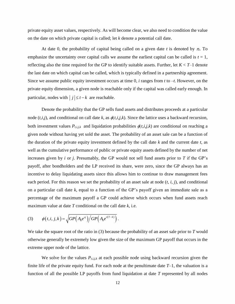
Denote the probability that the GP sells fund assets and distributes proceeds at a particular
node (t,i,j), and conditional on call date k, as t,i,j,k). Since the lattice uses a backward recursion,
both investment values Pt,i,j,k and liquidation probabilities t,i,j,k) are conditional on reaching a
given node without having yet sold the asset. The probability of an asset sale can be a function of
the duration of the private equity investment defined by the call date k and the current date t, as
well as the cumulative performance of public or private equity assets defined by the number of net
increases given by i or j. Presumably, the GP would not sell fund assets prior to T if the GP’s
payoff, after bondholders and the LP received its share, were zero, since the GP always has an
incentive to delay liquidating assets since this allows him to continue to draw management fees
each period. For this reason we set the probability of an asset sale at node (t, i, j), and conditional
on a particular call date k, equal to a function of the GP’s payoff given an immediate sale as a
percentage of the maximum payoff a GP could achieve which occurs when fund assets reach
maximum value at date T conditional on the call date k, i.e.
(3) .
We take the square root of the ratio in (3) because the probability of an asset sale prior to T would
otherwise generally be extremely low given the size of the maximum GP payoff that occurs in the
extreme upper node of the lattice.
We solve for the values Pt,i,j,k at each possible node using backward recursion given the
finite life of the private equity fund. For each node at the penultimate date T–1, the valuation is a
function of all the possible LP payoffs from fund liquidation at date T represented by all nodes
j t k
0 0, , ,v T kvjt i j k GP A e GP A e
13
which emanate from the node at T–1, exploiting the fact that the GP is sure to liquidate the private
equity portfolio at date T. Similarly, date T–2 values are obtained using all possible outcomes at
date T–1, except now these outcomes include both secondary market transactions as well as the
continuation values obtained in the prior step, and so on. Each value P is a certainty equivalent,
that is, the value of a risk-free bond that provides the same utility for sure as the expected utility
of the investment the following period.
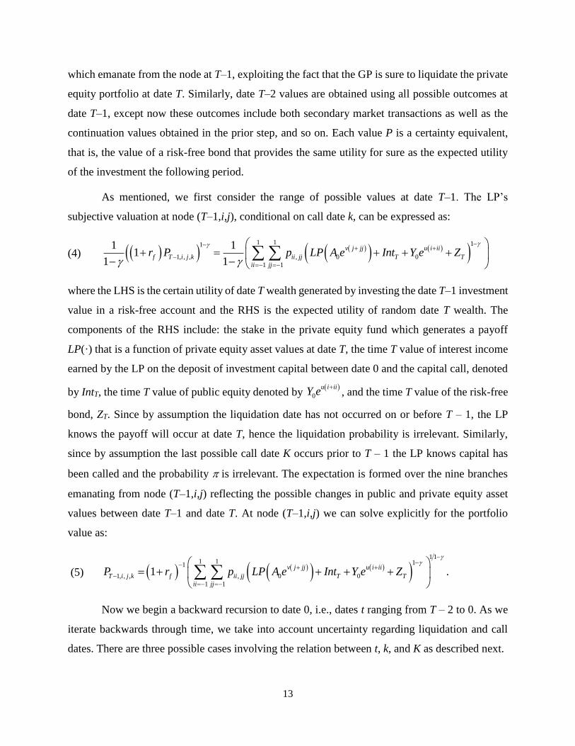
As mentioned, we first consider the range of possible values at date T–1. The LP’s
subjective valuation at node (T–1,i,j), conditional on call date k, can be expressed as:
(4)
where the LHS is the certain utility of date T wealth generated by investing the date T–1 investment
value in a risk-free account and the RHS is the expected utility of random date T wealth. The
components of the RHS include: the stake in the private equity fund which generates a payoff
LP(·) that is a function of private equity asset values at date T, the time T value of interest income
earned by the LP on the deposit of investment capital between date 0 and the capital call, denoted
by IntT, the time T value of public equity denoted by , and the time T value of the risk-free
bond, ZT. Since by assumption the liquidation date has not occurred on or before T – 1, the LP
knows the payoff will occur at date T, hence the liquidation probability is irrelevant. Similarly,
since by assumption the last possible call date K occurs prior to T – 1 the LP knows capital has
been called and the probability is irrelevant. The expectation is formed over the nine branches
emanating from node (T–1,i,j) reflecting the possible changes in public and private equity asset
values between date T–1 and date T. At node (T–1,i,j) we can solve explicitly for the portfolio
value as:
(5)
Now we begin a backward recursion to date 0, i.e., dates t ranging from T – 2 to 0. As we
iterate backwards through time, we take into account uncertainty regarding liquidation and call
dates. There are three possible cases involving the relation between t, k, and K as described next.
1 1 11
1, , , , 0 0
1 1
1 11
1 1
v j jj u i ii
f T i j k ii jj T T
ii jj
r P p LP A e Int Y e Z
0
u i iiY e
1 1
1 1 11
1, , , , 0 0
1 1
1 .v j jj u i ii
T i j k f ii jj T T
ii jj
P r p LP A e Int Y e Z
14
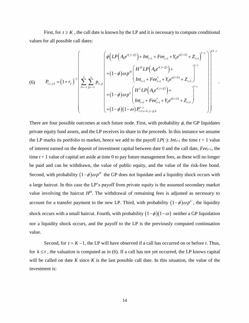
First, for , the call date is known by the LP and it is necessary to compute conditional
values for all possible call dates:
(6)
There are four possible outcomes at each future node. First, with probability , the GP liquidates
private equity fund assets, and the LP receives its share in the proceeds. In this instance we assume
the LP marks its portfolio to market, hence we add to the payoff LP(·): Intt+1 the time t + 1 value
of interest earned on the deposit of investment capital between date 0 and the call date, Feet+1, the
time t + 1 value of capital set aside at time 0 to pay future management fees, as these will no longer
be paid and can be withdrawn, the value of public equity, and the value of the risk-free bond.
Second, with probability the GP does not liquidate and a liquidity shock occurs with
a large haircut. In this case the LP’s payoff from private equity is the assumed secondary market
value involving the haircut HH. The withdrawal of remaining fees is adjusted as necessary to
account for a transfer payment to the new LP. Third, with probability , the liquidity
shock occurs with a small haircut. Fourth, with probability neither a GP liquidation
nor a liquidity shock occurs, and the payoff to the LP is the previously computed continuation
value.
Second, for , the LP will have observed if a call has occurred on or before t. Thus,
for , the valuation is computed as in (6). If a call has not yet occurred, the LP knows capital
will be called on date K since K is the last possible call date. In this situation, the value of the
investment is:
t K
1
0 1 1 0 1
1
0
1 *11 1 0 1
, , , ,11
0
*
1 1 0 1
1,
1
1
1
1 1
v j jj u i ii
t t t
v j jjH
H
u i ii
t t tt i j k f ii jj
jj v j jjL
L
u i ii
t t t
t
LP A e Int Fee Y e Z
H LP A ep
Int Fee Y e ZP r p
H LP A ep
Int Fee Y e Z
P
1 1
1
1
1
, ,
.ii
i ii j jj k
1 Hp
1 Lp
1 1
1t K
k t
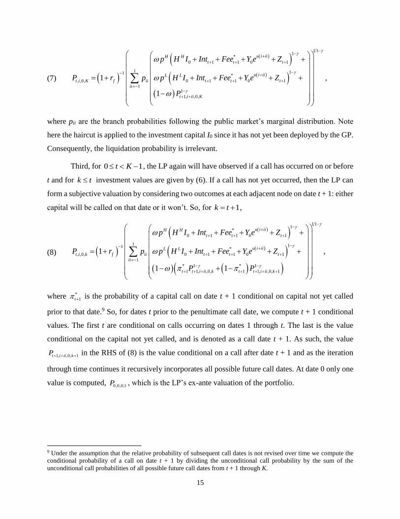
15
(7)
where pii are the branch probabilities following the public market’s marginal distribution. Note
here the haircut is applied to the investment capital I0 since it has not yet been deployed by the GP.
Consequently, the liquidation probability is irrelevant.
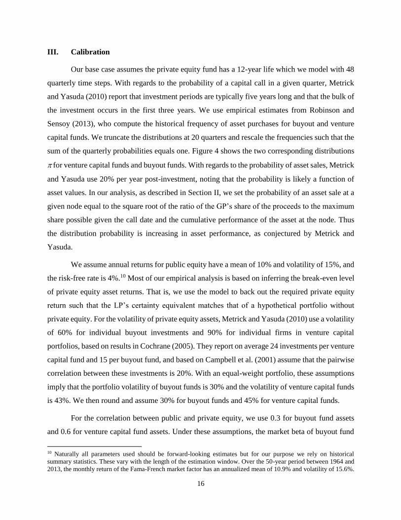
Third, for , the LP again will have observed if a call has occurred on or before
t and for investment values are given by (6). If a call has not yet occurred, then the LP can
form a subjective valuation by considering two outcomes at each adjacent node on date t + 1: either
capital will be called on that date or it won’t. So, for ,
(8)
where is the probability of a capital call on date t + 1 conditional on capital not yet called
prior to that date.9 So, for dates t prior to the penultimate call date, we compute t + 1 conditional
values. The first t are conditional on calls occurring on dates 1 through t. The last is the value
conditional on the capital not yet called, and is denoted as a call date t + 1. As such, the value
in the RHS of (8) is the value conditional on a call after date t + 1 and as the iteration
through time continues it recursively incorporates all possible future call dates. At date 0 only one
value is computed, , which is the LP’s ex-ante valuation of the portfolio.
9 Under the assumption that the relative probability of subsequent call dates is not revised over time we compute the
conditional probability of a call on date t + 1 by dividing the unconditional call probability by the sum of the
unconditional call probabilities of all possible future call dates from t + 1 through K.
1 11
*
0 1 1 0 1
1 11*
, ,0, 0 1 1 0 1
11
1, ,0,
1 ,
1
u i iiH H
t t t
u i iiL L
t i K f ii t t t
ii
t i ii K
p H I Int Fee Y e Z
P r p p H I Int Fee Y e Z
P
0 1t K
k t
1k t
1 11
*
0 1 1 0 1
1 11*
, ,0, 0 1 1 0 1
1
* 1 * 1
1 1, ,0, 1 1, ,0, 1
1 ,
1 1
u i iiH H
t t t
u i iiL L
t i k f ii t t t
ii
t t i ii k t t i ii k
p H I Int Fee Y e Z
P r p p H I Int Fee Y e Z
P P
*
1t
1, ,0, 1t i ii kP
0,0,0,1P
16
III. Calibration
Our base case assumes the private equity fund has a 12-year life which we model with 48
quarterly time steps. With regards to the probability of a capital call in a given quarter, Metrick
and Yasuda (2010) report that investment periods are typically five years long and that the bulk of
the investment occurs in the first three years. We use empirical estimates from Robinson and
Sensoy (2013), who compute the historical frequency of asset purchases for buyout and venture
capital funds. We truncate the distributions at 20 quarters and rescale the frequencies such that the
sum of the quarterly probabilities equals one. Figure 4 shows the two corresponding distributions
for venture capital funds and buyout funds. With regards to the probability of asset sales, Metrick
and Yasuda use 20% per year post-investment, noting that the probability is likely a function of
asset values. In our analysis, as described in Section II, we set the probability of an asset sale at a
given node equal to the square root of the ratio of the GP’s share of the proceeds to the maximum
share possible given the call date and the cumulative performance of the asset at the node. Thus
the distribution probability is increasing in asset performance, as conjectured by Metrick and
Yasuda.
We assume annual returns for public equity have a mean of 10% and volatility of 15%, and
the risk-free rate is 4%.10 Most of our empirical analysis is based on inferring the break-even level
of private equity asset returns. That is, we use the model to back out the required private equity
return such that the LP’s certainty equivalent matches that of a hypothetical portfolio without
private equity. For the volatility of private equity assets, Metrick and Yasuda (2010) use a volatility
of 60% for individual buyout investments and 90% for individual firms in venture capital
portfolios, based on results in Cochrane (2005). They report on average 24 investments per venture
capital fund and 15 per buyout fund, and based on Campbell et al. (2001) assume that the pairwise
correlation between these investments is 20%. With an equal-weight portfolio, these assumptions
imply that the portfolio volatility of buyout funds is 30% and the volatility of venture capital funds
is 43%. We then round and assume 30% for buyout funds and 45% for venture capital funds.
For the correlation between public and private equity, we use 0.3 for buyout fund assets
and 0.6 for venture capital fund assets. Under these assumptions, the market beta of buyout fund
10 Naturally all parameters used should be forward-looking estimates but for our purpose we rely on historical
summary statistics. These vary with the length of the estimation window. Over the 50-year period between 1964 and
2013, the monthly return of the Fama-French market factor has an annualized mean of 10.9% and volatility of 15.6%.
17
assets is 0.6 (so the levered fund beta is 1.2 at 1X leverage) and of venture capital fund assets is
1.8. These betas are correspond closely to empirical estimates of the betas of private equity funds,
which are typically around one for (levered) buyout betas and two for venture capital funds.11
To illustrate the lattice topology with quarterly time steps, we use the base-case mean and
volatility for annual public equity returns of 10% and 15%, respectively. For venture capital and
buyout funds we use asset volatilities of 45% and 30%, respectively, and correlations with public
equity of 0.6 and 0.3. For both we use an asset expected return of 20%. Listed in Table A1 in the
Appendix are branch probabilities determined to generate a discrete trinomial distribution that
matches the mean and volatility of each normal distribution. Our procedure described in Appendix
1 results in quarterly step sizes of 9.8% for public equity, 30.9% for venture capital funds, and
19.6% for buyout funds. In panel A, listed for public equity is the marginal probability of each of
the three possible returns and listed for the venture capital fund is the conditional probability of
each of the three possible returns given one of the public equity returns. Note that the conditional
volatility of venture capital fund asset returns is equal in all cases, since the bivariate normal
distribution implies a conditional volatility equal to the unconditional volatility scaled by
. The conditional mean of venture capital fund assets is substantially affected by the return of
public equity. The conditional mean following a positive public equity return, for example, is
18.2% on a quarterly basis versus –17.2% following a negative public equity return. Panel B shows
the corresponding calculations for buyout funds. Note that joint probabilities are higher along the
diagonal for venture capital funds reflecting the higher assumed correlation.
The tight match between the discrete distribution of the lattice and the assumed continuous
distribution is illustrated in Figure 5, which shows the probability of landing on each node at time
T = 48 as well as the corresponding probability from the bivariate normal distribution.
We assume that liquidity shocks are rare events with base-case probability equal to 1%
per quarter, consistent with the estimate of a global consumption shock in Nakamura et al. (2013)
of 3.7% per annum. We change the probability in the lattice at date t by increasing by 1% for
every net decrease in public equity asset value between date 0 and t. For nodes with a net increase
11 See Cochrane (2005), Korteweg and Sorensen (2010), and Driessen et al. (2010).
21
18
in asset value we leave at 1%. The intuition is that an LP is more likely to suffer a liquidity crisis
when its relatively more liquid assets are declining in value.
For GP fees we assume a 2% management fee, a 20% performance fee, and an 8% hurdle
rate, all of which are typical as found in Metrick and Yasuda (2010).
With regards to LP risk aversion, Mehra and Prescott (1985) review the use of in prior
literature, state that most studies use values between one and two, and argue that the parameter
should be restricted to a maximum of ten. More recently, Campbell and Cochrane (1999) set
equal to two in their seminal work on consumption-based asset pricing. As described in the
following section, we find that for a 12-year investment horizon, and our assumptions about the
risk-free rate and public equity’s expected return and volatility, values for between 1.5 and 3.5
generate reasonable optimal asset allocations. Hence, these are the values we use throughout the
paper.
Table 1 summarizes the base case assumptions for each of the parameters of the model.
IV. Results
IV.A. Benchmark Portfolio of Public Equity and a Risk-free Bond
In much of our analysis it will be helpful to have a benchmark based on public equity for
comparison. Consider an investor with a 12-year investment horizon. Using the same type of
trinomial lattice described in Section II, and our base-case assumptions about the risk-free rate and
the expected return of public equity, we determine the allocation weights across public equity and
risk-free bonds that maximizes the certainty equivalent of the portfolio, over a range of risk
aversion levels and public equity volatility. We restrict allocation to public equity to be no greater
than 100%. Figure 6 shows the results. For low levels of risk aversion and volatility the investor
should invest all wealth in public equity. For volatility of 15%, which is typical of estimates of
long-run volatility for the stock market, optimal allocation is 100% for = 3 and below. However,
given short-term liquidity needs, all investors hold some fraction of wealth in the risk-free asset.
In the 2014 NACUBO study of university endowments, for example, the typical endowment
allocates roughly 20% to cash and bonds, hence for our benchmark we assume a 20% allocation
to the risk-free bond with the remaining 80% split between public and private equity.
19
IV.B. Impact of Stochastic Capital Calls and Distributions
As mentioned previously, prior academic work abstracts from the uncertainty of timing of
LP cash flows in private equity funds. In this subsection we focus on uncertainty regarding the
dates of capital calls and the return of equity capital by the GP, and show that this uncertainty has
a significant impact on LP valuations. To illustrate this point, we assume here that there are no
liquidity shocks or secondary sales, and focus on the simpler case in which the LP does not invest
in public equities. These simplifications allow us to directly associate changes in assumptions
about calls and distributions to resulting changes in private equity valuations.
Consider an LP with a risk aversion parameter of 2.5 who invests in a portfolio of 80%
private equity and 20% in risk-free bonds.12 We evaluate the LP’s ex-ante certainty equivalent
value of this portfolio under different assumptions about private equity cash flow timing, reported
in Table 2. We do so for three possible private equity funds: a venture capital fund (Panel A), a
“1X” buyout fund with debt equal to 100% of initial equity (Panel B), and a “3X” buyout fund
with debt equal to 300% of initial equity (Panel C). As described in Section III, we use an expected
return and volatility of public equities of 10% and 15%, respectively, and a volatility of 45% and
30%, respectively, for venture capital and buyout fund assets. The risk-free rate is 4%.
In the benchmark case, reported in the first column of Table 2, capital is called immediately
at t=0 and the distribution occurs at the end of the fund’s 12-year life (date T), consistent with
Sorensen et al. (2014). Here, we calibrate the expected return of private equity assets so that the
portfolio’s value is exactly equal to a portfolio of 80% public equity and 20% risk-free bonds,
hence by construction the certainty equivalent is the same in the first column in all three panels.
This certainty equivalent is roughly 161% of LP wealth, far in excess of 100% indicating that
public equity is attractive to this LP. The required annual expected returns are 20.6% for venture
capital funds, 17.3% for 1X buyout funds, and 18.4% for 3X buyout funds. We use these expected
returns in all other columns to assure comparability.
In the second column of Table 2 the capital call occurs at the end of 2.5 years instead of at
t=0, reflecting the time spent by the GP in identifying suitable investments. The distribution date
12 The bond allocation can be interpreted as optimally trading off risk and return as well as accommodating short-term
liquidity needs as discussed above. The position in riskless bonds also avoids cases in which the LP receives a payoff
of zero in a levered fund when terminal asset values are less than the amount owed to debt investors – given the
assumed utility function these cases have a dramatic effect on valuation.
20
remains fixed but occurs prior to year 12. For venture capital funds the distribution occurs at the
end of 11.25 years for a total investment horizon of 8.75 years, and for buyout funds the
distribution occurs at the end of 9.25 years for a total investment horizon of 6.75 years. These
distribution dates are chosen to match those which arise endogenously in the fourth and fifth
columns, as described below, so that we can make informative comparisons. In practice, portfolio
company holding periods are indeed substantially shorter than the contracted life of the fund as
investments are made by the GP over the first few years of the fund’s life and exited when the GP
decides to do so. Stromberg (2009) reports typical investment horizons for buyout fund assets in
the range of 5 to 7 years; typical holding periods for venture capital assets are likely to be somewhat
longer given their early stage. The more realistic shorter investment horizons in columns two
through five compared to the first column results in a substantially decreased valuations for all
types of funds, as the private equity assets have less time to increase in value.
In the third column we hold distributions fixed as in the second column, and introduce
stochastic capital calls by assuming that capital is called with equal probability each quarter over
the first 4.75 years, resulting in an expected delay of 2.5 years. Although the expected call date is
the same as in the second column, introducing uncertainty in this way lowers the LP’s subjective
portfolio value by about 1% of initial wealth, for all fund types.
In the fourth and fifth columns we allow stochastic distributions following the expression
in (3), with the timing of capital calls the same as in the second and third columns, respectively.
The resulting holding periods are endogenously determined as a consequence of the GP’s
distribution rule and as mentioned are about 8.75 years for venture capital funds and 6.75 for
buyout funds. Here, we see that the LP’s value is considerably larger than in the cases with fixed
distributions. The GP’s rule makes distributions more likely when the private equity asset value is
high while the fixed distribution does not. This outweighs the negative effect on valuation of the
pure uncertainty. As before, moving from fixed to stochastic capital calls lowers the LP’s value.
Overall, the main message from Table 2 is that stochastic capital calls and distributions,
unexplored in prior work, have a significant impact on the ex-ante value of private equity funds.
Uncertainty in the timing of cash flows generally lowers the risk-averse LP’s certainty equivalent,
21
but this is offset in the case of distributions by an endogenous GP decision rule that makes higher-
value outcomes more likely.13
IV.C. Impact of Liquidity Shocks and Secondary Market Discounts
In this subsection we focus on the impact of liquidity shocks and secondary market
discounts on private equity values. As above, we assume here the LP does not allocate across
public and private equity. However, we use a three-dimensional lattice that models the joint
evolution of public and private equity in order to incorporate the relation between public equity
performance and both the probability of a liquidity crisis and the probability that haircuts are in a
high or low state.
In Figure 7 we show certainty equivalents of private equity investments when the LP is
vulnerable to liquidity shocks and must sell at a discount on the secondary market when a liquidity
shock arrives. Liquidity shocks occur at a base rate of 1% per quarter, with rates increasing as
public equity values fall as described in Section II. To measure the impact of the size of the haircut
on valuations we show results for Small Haircuts, with HH = 90% and HL = 95%, and Large
Haircuts, with HH = 50% and HL = 90%. Certainty equivalents are computed over a range of
expected asset returns. As before we compute certainty equivalents for portfolios of 80% private
equity and 20% risk-free bonds. We show results for venture capital funds, with asset volatility of
45% and no leverage, and buyout funds, with asset volatility of 30% and either 1X or 3X leverage.
Figures A through C show results for less risk averse investors with = 1.5 and Figures D through
F show results for more risk averse investors with = 2.5. Naturally in all cases certainty
equivalents are increasing in asset expected return. More importantly, the gap between certainty
equivalents for Small and Large Haircuts is substantial and widens as expected returns increase.
For higher risk aversion, the difference reaches a maximum of roughly 25% for all three fund
types. For lower risk aversion, the difference is not as large but still reaches a maximum of roughly
15% for all three fund types. These results indicate that the efficiency of the secondary market for
private equity investments has a significant impact on their valuation.
Perhaps the most important question facing LPs is what rate of return is required to
compensate for the risk of underlying assets, the uncertainty of the timing of cash flows in private
13 All expected returns are constant over time in the model, so there is no sense in which capital calls can be strategic,
e.g. to take advantage of depressed asset prices.

22
equity funds, as well as the size of the haircut required to transact in the secondary market. Our
methodology takes as an input the expected return of private equity asset values, and by varying
this input we can quickly determine using numerical methods the return required to generate a
break-even valuation. For this analysis we use as a benchmark the certainty equivalent of a
portfolio of 80% public equity, with expected return of 10% and volatility of 15%, and 20% in
risk-free bonds with a return of 4%. The private equity investments are also portfolios with a 20%
allocation to risk-free bonds. Thus, these analyses compute the expected return on private equity
assets needed to make the LP indifferent to replacing a portfolio that is 80% public equity and 20%
risk-free bonds with one that is 80% private equity and 20% risk-free bonds.14 Of course, investors
hold private equity in a well-diversified portfolio, and we explore below how breakeven returns
change when we allow portfolios to mix public and private equity. For both public and private
equity we incorporate the impact of liquidity shocks and corresponding secondary market
transactions; the difference between the two is that public equity is exited at NAV whereas private
equity sales entail a haircut.
Table 3 reports the break-even expected asset returns in venture capital funds in Panel A,
as a function of LP risk aversion and the size of the haircut parameters HH and HL. In all cases the
break-even return is increasing in risk aversion and decreasing in the prices available in the
secondary market as modeled by the haircuts. Risk aversion has a first-order impact on break-even
returns suggesting that venture capital funds are appropriate as a stand-alone investment for only
a subset of potential investors. For the least risk averse LP, the breakeven asset returns range from
18.0% at the most efficient secondary market (HL = 95% and HH = 90%) to 19.9% for the least
efficient secondary market (HL = 90% and HH = 50%). The difference of 1.9% annually is one
measure of the cost of inefficient secondary markets for venture capital funds. For the most risk
averse LP, the breakeven asset returns range from 29.4% to 39.7% across the efficiency
parameters. The efficiency of the secondary market clearly affects the attractiveness of private
equity.
14 This is a tougher, but more appropriate, benchmark than requiring that the portfolio involving private equity simply
have a certainty-equivalent at least equal to the LP’s wealth. A benchmark of the LP’s wealth would be appropriate if
the alternative investment were a portfolio of 100% riskless bonds; as shown in Figure 5 and Table 2, the LP can
achieve a higher certainty equivalent by investing in public equities.
23
Another metric for performance is the break-even alpha of fund assets, which is straight-
forward to compute by subtracting from a break-even asset return the corresponding expected
return from a single factor model. We use public equity as a proxy for the single factor. As
described in Section III, our base case assumptions result in a venture capital asset beta of 1.8
which implies an expected asset return of 14.8%, assuming a 4% risk-free rate and 10% expected
return for public equity. Similarly, for buyout assets, the beta is 0.6 which implies an expected
return of 7.6%. Panel B lists the break-even alphas for venture capital assets. The impact of the
secondary market efficiency is modest for the lowest risk aversion, but extreme for the most risk-
averse, suggesting that for many investors it is unlikely that venture capital funds are appropriate
when secondary markets are inefficient.
Panel C shows the realized LP returns that correspond to the break-even asset returns in
Panel A. The break-even LP returns are more salient since they can be compared to historical LP
returns to assess whether private equity funds have in the past generated sufficient returns to
compensate investors for risk and various costs. Given the uncertain call and distribution dates in
private equity funds, there are a number of different ways that realized returns can be computed.
For example, for a given investment horizon T, the LP’s capital is only deployed by the manager
for the time between call and distribution dates, and assumptions are required to account for the
periods outside this window. To facilitate comparisons to reported LP performance, which
typically assume fund exits only occur when the GP distributes, we compute LP fund returns
assuming there are no liquidity shocks and associated secondary market transactions. Since
different paths through the lattice can still result in different exit dates from the fund, we first
compute the IRR on a quarterly basis that sets the present value of the payoff equal to the initial
committed capital. Next, we compute a median IRR taking into account the likelihood of each
possible payoff occurring in the lattice.15
As seen in Panel C, the relation between the LP’s break-even return, risk aversion, and the
haircut parameters is qualitatively the same as in Panel A. One other result stands out: the break-
even LP return is roughly 70% of gross return of fund assets, reflecting the substantial share of
gross fund performance that accrues to the GP. For comparison, Harris et al. (2014) report an
average IRR for LPs in venture capital funds of 16.8%, indicating that the average venture capital
15 We focus on median performance metrics due to the presence of influential outliers at the extremes of the lattice.
24
fund in their sample generated returns that exceed the break-even returns in Table 3 from the
perspective of the least risk-averse investor but fell short otherwise, even with highly efficient
secondary markets. Common performance metrics for private equity funds are the TVPI, discussed
previously, and the Public Market Equivalent (PME). In this exercise we compute a median TVPI
using the distribution of gross returns from the set of possible payoffs in the lattice. We compute
PMEs by scaling each possible payoff at date t by the future value at t of the committed capital
grossed up by the public equity return that occurred over that particular path. Panels D and E show
the median TVPI and PME, respectively, which correspond to the break-even asset returns in Panel
A. As before, break-even TVPI and PME are substantially affected by the efficiency of the
secondary market, especially for the more risk-averse investor. The break-even PME, for example,
falls from 3.20 to 2.22 for the medium risk-averse investor as markets are made more efficient.
For comparison, Harris et al. (2014) report average PMEs of 1.22 for buyout funds and 1.36 for
venture capital funds. Here the average fund underperforms our model-implied break-even PME
in almost all cases.
Table 4 shows break-even asset returns and LP returns for a 1X buyout fund. Assets have
annual volatility of 30%. Break-even asset returns are slightly lower than the venture capital fund
results in Table 3. In contrast, break-even fund returns are in almost all cases somewhat higher,
indicating that for the utility function considered, the levered investment in the lower volatility
assets of the buyout fund is riskier for the LP than the unlevered investment in the higher volatility
assets of the venture capital fund. For the least risk averse investor and the most efficient secondary
market, for example, the break-even venture capital fund returns is 14.3% versus 16.0% for the
buyout fund. Table 5 shows break-even returns for a 3X buyout fund. In all cases the break-even
fund returns are substantially higher than in Table 4, as one would expect for the additional risk
generated by leverage. The difference is much larger for the highest level of risk aversion. For the
most efficient secondary market, for example, the break-even fund return is 27.6% for lower
leverage and 39.2% for higher leverage. The average IRR of buyout funds in Harris et al. (2014)
is 14.2%. Regardless of the haircuts, risk aversion, and leverage, this indicates that the average
buyout fund in their sample underperformed relative to our model’s benchmark.
One feature of private equity funds that drives a wedge between the asset return, i.e., the
return of underlying portfolio companies, and the return experienced by an LP is the fee structure
charged by GPs. The most common is a 2% annual management fee and 20% carried interest, the
25
base case assumptions in this paper. To illustrate the impact of fees on the returns earned by LPs,
we repeat the break-even analysis described above for the LP with = 1.5. Table 6 shows results
for each fund type across a range of management fees and levels of carried interest. In Panels A
and B, corresponding to venture capital and 1X buyout funds, the maximum fees increase the
break-even asset return by roughly 8% per annum. In Panel C, for 3X buyout funds, the required
asset return increases by about 5%.
IV.D. Allocation across Public and Private Equity
The valuation and break-even analyses in the prior subsections involve portfolios of private
equity and a risk-free bond. While this setup is useful for isolating the impact of the efficiency of
the secondary market, it ignores diversification between public and private equity markets. In this
section we examine a portfolio of risk-free bonds, public equity, and either buyout or venture
capital funds to provide additional insight in a context resembling the endowment of an
institutional investor.
Following the throes of the Great Recession, public equity has generated high returns from
a historical perspective, resulting in some investors reducing their allocation to other asset
classes.16 One way to frame the analysis is to determine the minimum expected return of a private
equity fund such that an investor is indifferent between a portfolio with no private equity and one
with a given allocation to private equity. We assume a 20% allocation to risk-free bonds earning
4% in all cases to accommodate an institution’s immediate liquidity needs. For a given level of
risk aversion, we then compute the certainty equivalent of a portfolio that is 80% allocated to
public equity with expected return of 10% and volatility of 15%. Next, we numerically determine
the expected asset return for private equity such that a portfolio that is either 20%, 40%, or 60%
allocated to private equity (with corresponding allocation of 60%, 40%, and 20% to public equity)
generates the same certainty equivalent as the 80% allocation to public equity.
Results are displayed in Table 7 across sets of allocation and haircut parameters for venture
capital funds with no leverage and assets with volatility of 45%. In Panel A, though increasing the
allocation to private equity can generate a larger diversification benefit, the increased risk
generates in all cases a monotonic relationship between the allocation to venture capital and the
16 For example, see “Calpers to Exit Hedge Funds” Wall Street Journal 9/15/14.
26
required expected asset return. Perhaps most salient for our study, comparing break-even fund
returns across secondary market parameters gives a measure of the LP’s cost of illiquidity in a
portfolio context. The difference is as narrow as 2.0% per annum ( = 1.5 and x = 20%) to as high
as 5.7% per annum ( = 3.5 and x = 60%).
Comparing these results to those in Table 3 shows that break-even venture capital fund
returns are substantially lower in a portfolio context. For investors with = 2.5, for example, and
when secondary markets are least efficient, the break-even fund return in Panel C of Table 3 is
20.6%, and this drops to just 12.4% when allocation to venture capital is 20% in Panel C of Table
8. Viewed in this way, the typical fund in empirical studies such as Harris et al. (2014) is closer to
our benchmark. Note that our procedure allows an individual LP to determine its own benchmark
given an estimate of risk aversion, the LP’s chosen allocation to venture capital, and the other
parameters of our model.
Tables 8 and 9 show corresponding results for 1X buyout funds and 3X buyout funds,
respectively, both with asset volatility of 30%. The additional leverage has little impact on break-
even fund returns for investors with = 1.5. For more risk-averse investors, additional leverage
raises the break-even fund return substantially for larger allocations, with a difference of 7.1% per
annum, 17.3% for 1X leverage and 24.4% for 3X leverage, for the largest allocation and a more
efficient secondary market. A similar pattern exists for TVPI and PME in Panels D and E,
respectively, in the two tables.
Our last analysis fixes the bond allocation to 20% and then finds the utility-maximizing
split between public and private equity. We do this for each type of private equity fund at the most
efficient and least efficient secondary market parameters. Results are displayed in Table 10. In
Panel A, for the least risk-averse investor, the optimal allocation to venture capital increases from
27% to 37% when secondary markets are made more efficient. For the most risk-averse investor
the increase is smaller in absolute terms but larger in percentage terms, rising from 6% to 11%.
This result indicates that the efficiency of the secondary market has a substantial effect on the
optimal portfolio. Also, the optimal allocation to venture capital is widely varying across risk-
aversion levels. Results in Panels B and C are qualitatively similar. Interestingly, as reported in
the 2015 NACUBO study, the allocations in the less efficient secondary market case correspond
27
to the average allocation to alternative investments in 2014 for university endowments as a
function of the size of the endowment.
VI. Conclusion
This paper presents a valuation framework for private equity investment from the
perspective of a risk-averse LP, explicitly incorporating institutional features that differentiate
private equity from other types of vehicles. In particular, we allow for a distribution of call dates
thereby reflecting the uncertainty of how long capital is actually deployed in private equity assets.
We also allow for uncertainty surrounding when assets are liquidated by the GP. Most importantly,
we model LP exits on a secondary market in response to liquidity shocks. Secondary markets are
quickly developing in practice to remedy the severe illiquidity in private equity investment. Up
until now, there has been no research that studies the impact of the efficiency of secondary markets
on the valuation of private equity stakes.
We find that cash flow uncertainty does matter, both by reducing the average time that
capital is deployed by GPs as well as creating additional uncertainty in the distribution of LP
payoffs. In our model, we assume that LPs set aside all committed capital at date 0 in an interest-
bearing account, hence a distribution of call dates naturally leads to periods of low earning power
for LPs. We also find that the efficiency of the secondary market can have a dramatic impact on
the attractiveness of private equity investment, in some cases reducing the break-even fund return
by 10% per year.
Our model can be used to guide LPs in their ex-ante allocation decision, as well as ex-post
analysis of performance. In both cases our procedure requires as an input the LP’s assessment of
the distribution of call dates as well as the subsequent likelihood of a GP’s distribution of fund
proceeds. These parameters can be studied using historical data of LP cash flows.
We make a number of simplifications to our representation of an LP’s decision problem to
gain tractability, and at least two of these we plan on relaxing in future work.
First, for a given private equity investment, we assume that all committed capital is called
on a single date, and all fund assets are liquidated on a single subsequent date. This assumption
likely overstates the cost of illiquidity, since in practice LPs hold a portfolio of private equity

28
investments, with partial calls and liquidations for each, so that the allocation to private equity in
whole is somewhat self-financing. That said, the popular press has documented cases in which the
systematic component of calls and distributions has left LPs with significant liquidity crises. In
future work we plan on incorporating multiple calls and distributions.
Second, we assume the LP has an investment horizon equal to the contracted life of a single
private equity investment. Our valuation model therefore focuses on this relatively short time
period. In practice, private equity investors often have a very long investment horizon. For
University endowments, for example, one could argue the relevant horizon is infinite given the
permanent role that endowments can play in a University’s budget. In subsequent work, we plan
on fixing the investment horizon at some arbitrarily long horizon and allowing LPs to roll over
distributions from private equity investments into new commitments.
In both cases, relaxing these assumptions will likely increase the dimensionality of the
valuation, resulting in the need for large-scale parallel processing to generate numerical solutions.
29
Appendix
A.1. Waterfall
The computation of claimant shares follows closely that in Sorensen et al. (2014). Suppose
that fund assets are worth At on the liquidation date t. Distributions to the three types of claimants
are defined by three discrete asset levels denoted A1, A2, and A3. The first, A1, is the amount due
debt investors, i.e.
(A1)
Note that the value of the debt reflects the time from issuance, which is the call date k. We assume
that debt investors receive 100% of asset proceeds until they receive A1, the full amount they are
due. The second, A2, is defined by the LP’s hurdle rate h applied to the committed capital and all
management fees paid to the GP, i.e.
(A2)
Note that the hurdle rate is applied to the investment capital only from the call date k, whereas the
hurdle rate is applied to all management fees paid beginning on date 1. We assume that, once the
debt investors are fully repaid, the LP receives 100% of additional asset proceeds until they receive
A2 – A1.
The third, A3, is defined by the GP’s carried interest, c, which is a percentage of fund
profits, typically 20%, as follows:
(A3) .
The left-hand side of (A3) is the GP’s contractual carried interest payment and the right-
hand side of (4) is the “catch-up” region of asset sales, assuming that the GP receives 100% of
proceeds beyond A2 until its carried interest is paid. The solution to (A3) is
. Beyond A3, asset sale proceeds are split between the LP and GP
with the GP receiving a fraction c of the incremental proceeds.
A.2. Branch Probabilities
When considering private equity (V) investment as a stand-alone investment we assume
returns over each period of length t are normally distributed
(A4)
where and are annual mean and volatility, respectively. Following Kamrad and Ritchken
(1991) we can approximate the continuous normal distribution of using a discrete random
variable governed by the trinomial distribution used in the lattice. From any node in the lattice,
the discrete variable can take on one of three values
(A5)
where scales the familiar Cox, Ross, and Rubenstein (1979) binomial lattice step size. The
free parameter is selected numerically to both ensure all probabilities between 0 and 1 and to
keep the three branch probabilities as close to 1/3 as possible to aid the ability of the discrete
1 0 1 .t k
fA D r
2 1 0 01 1 1 1 .
tt k t
f fA A I Yh m r r h
3 0 1 3 2c A Y A A A
3 2 0 1 1A A c Y A c
Vr
2~ , .V V Vr N t t
Vra
Vr
1
0
1
with probability
0 with probability
with probability
V V
a
V
V V
v t p
r p
v t p
1V
V
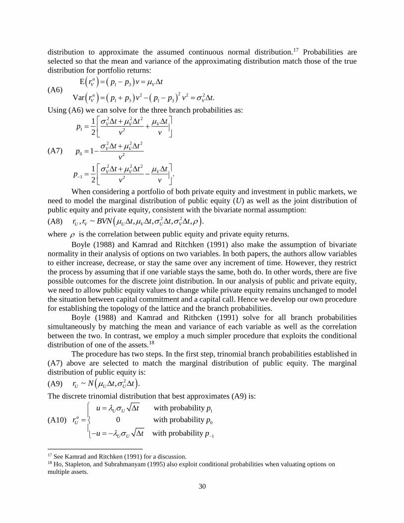
30
distribution to approximate the assumed continuous normal distribution.17 Probabilities are
selected so that the mean and variance of the approximating distribution match those of the true
distribution for portfolio returns:
(A6)
Using (A6) we can solve for the three branch probabilities as:
(A7)
When considering a portfolio of both private equity and investment in public markets, we
need to model the marginal distribution of public equity (U) as well as the joint distribution of
public equity and private equity, consistent with the bivariate normal assumption:
(A8)
where is the correlation between public equity and private equity returns.
Boyle (1988) and Kamrad and Ritchken (1991) also make the assumption of bivariate
normality in their analysis of options on two variables. In both papers, the authors allow variables
to either increase, decrease, or stay the same over any increment of time. However, they restrict
the process by assuming that if one variable stays the same, both do. In other words, there are five
possible outcomes for the discrete joint distribution. In our analysis of public and private equity,
we need to allow public equity values to change while private equity remains unchanged to model
the situation between capital commitment and a capital call. Hence we develop our own procedure
for establishing the topology of the lattice and the branch probabilities.
Boyle (1988) and Kamrad and Rithcken (1991) solve for all branch probabilities
simultaneously by matching the mean and variance of each variable as well as the correlation
between the two. In contrast, we employ a much simpler procedure that exploits the conditional
distribution of one of the assets.18
The procedure has two steps. In the first step, trinomial branch probabilities established in
(A7) above are selected to match the marginal distribution of public equity. The marginal
distribution of public equity is:
(A9)
The discrete trinomial distribution that best approximates (A9) is:
(A10)
17 See Kamrad and Ritchken (1991) for a discussion. 18 Ho, Stapleton, and Subrahmanyam (1995) also exploit conditional probabilities when valuating options on
multiple assets.
1 3
22 2 2
1 3 1 3
E
Var .
a
V V
a
V V
r p p v t
r p p v p p v t
2 2 2
1 2
2 2 2
0 2
2 2 2
1 2
1
2
1
1.
2
V V V
V V
V V V
t t tp
v v
t tp
v
t t tp
v v
2 2, ~ , , , , .U V U V U Vr r BVN t t t t
2~ , .U U Ur N t t
1
0
1
with probability
0 with probability
with probability
U U
a
U
U U
u t p
r p
u t p
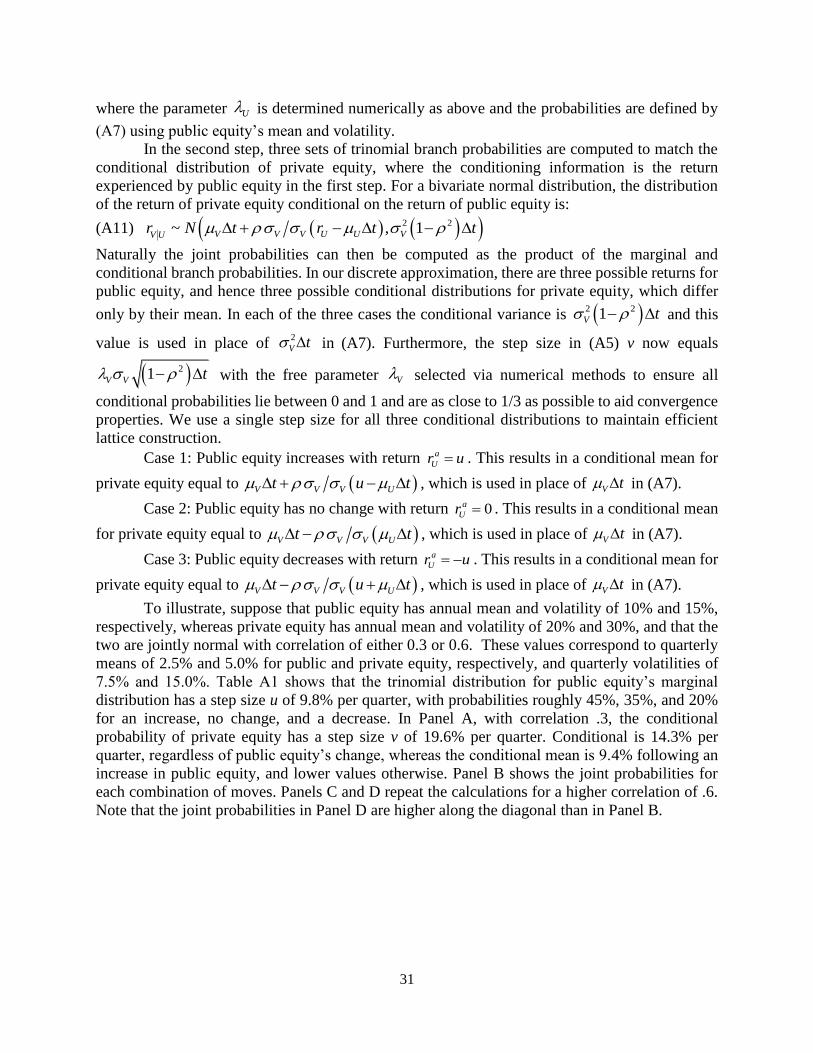
31
where the parameter is determined numerically as above and the probabilities are defined by
(A7) using public equity’s mean and volatility.
In the second step, three sets of trinomial branch probabilities are computed to match the
conditional distribution of private equity, where the conditioning information is the return
experienced by public equity in the first step. For a bivariate normal distribution, the distribution
of the return of private equity conditional on the return of public equity is:
(A11)
Naturally the joint probabilities can then be computed as the product of the marginal and
conditional branch probabilities. In our discrete approximation, there are three possible returns for
public equity, and hence three possible conditional distributions for private equity, which differ
only by their mean. In each of the three cases the conditional variance is and this
value is used in place of in (A7). Furthermore, the step size in (A5) v now equals
with the free parameter selected via numerical methods to ensure all
conditional probabilities lie between 0 and 1 and are as close to 1/3 as possible to aid convergence
properties. We use a single step size for all three conditional distributions to maintain efficient
lattice construction.
Case 1: Public equity increases with return . This results in a conditional mean for
private equity equal to , which is used in place of in (A7).
Case 2: Public equity has no change with return . This results in a conditional mean
for private equity equal to , which is used in place of in (A7).
Case 3: Public equity decreases with return . This results in a conditional mean for
private equity equal to , which is used in place of in (A7).
To illustrate, suppose that public equity has annual mean and volatility of 10% and 15%,
respectively, whereas private equity has annual mean and volatility of 20% and 30%, and that the
two are jointly normal with correlation of either 0.3 or 0.6. These values correspond to quarterly
means of 2.5% and 5.0% for public and private equity, respectively, and quarterly volatilities of
7.5% and 15.0%. Table A1 shows that the trinomial distribution for public equity’s marginal
distribution has a step size u of 9.8% per quarter, with probabilities roughly 45%, 35%, and 20%
for an increase, no change, and a decrease. In Panel A, with correlation .3, the conditional
probability of private equity has a step size v of 19.6% per quarter. Conditional is 14.3% per
quarter, regardless of public equity’s change, whereas the conditional mean is 9.4% following an
increase in public equity, and lower values otherwise. Panel B shows the joint probabilities for
each combination of moves. Panels C and D repeat the calculations for a higher correlation of .6.
Note that the joint probabilities in Panel D are higher along the diagonal than in Panel B.
U
2 2~ , 1V V V U U VV Ur N t r t t
2 21V t
2
V t
21V V t V
a
Ur u
V V V Ut u t V t
0a
Ur
V V V Ut t V t
a
Ur u
V V V Ut u t V t
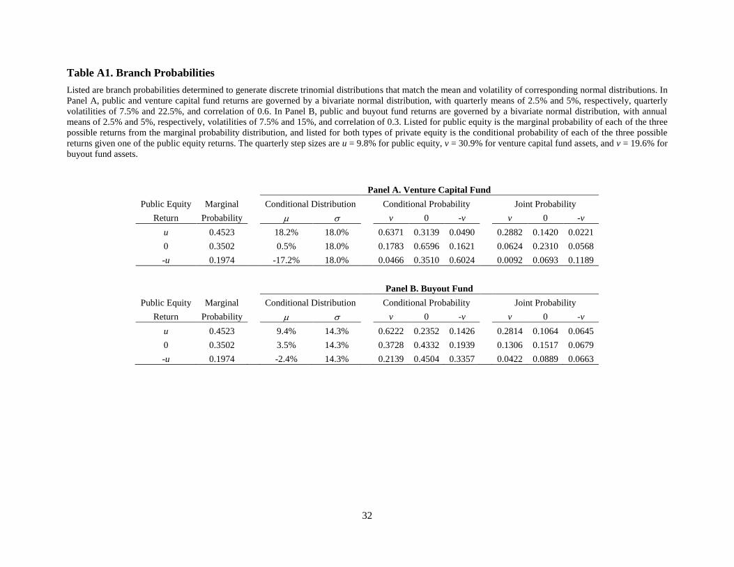
32
Table A1. Branch Probabilities
Listed are branch probabilities determined to generate discrete trinomial distributions that match the mean and volatility of corresponding normal distributions. In
Panel A, public and venture capital fund returns are governed by a bivariate normal distribution, with quarterly means of 2.5% and 5%, respectively, quarterly
volatilities of 7.5% and 22.5%, and correlation of 0.6. In Panel B, public and buyout fund returns are governed by a bivariate normal distribution, with annual
means of 2.5% and 5%, respectively, volatilities of 7.5% and 15%, and correlation of 0.3. Listed for public equity is the marginal probability of each of the three
possible returns from the marginal probability distribution, and listed for both types of private equity is the conditional probability of each of the three possible
returns given one of the public equity returns. The quarterly step sizes are u = 9.8% for public equity, v = 30.9% for venture capital fund assets, and v = 19.6% for
buyout fund assets.
Panel A. Venture Capital Fund
Public Equity Marginal Conditional Distribution Conditional Probability Joint Probability
Return Probability v 0 -v v 0 -v
u 0.4523 18.2% 18.0% 0.6371 0.3139 0.0490 0.2882 0.1420 0.0221
0 0.3502 0.5% 18.0% 0.1783 0.6596 0.1621 0.0624 0.2310 0.0568
-u 0.1974 -17.2% 18.0% 0.0466 0.3510 0.6024 0.0092 0.0693 0.1189
Panel B. Buyout Fund
Public Equity Marginal Conditional Distribution Conditional Probability Joint Probability
Return Probability v 0 -v v 0 -v
u 0.4523 9.4% 14.3% 0.6222 0.2352 0.1426 0.2814 0.1064 0.0645
0 0.3502 3.5% 14.3% 0.3728 0.4332 0.1939 0.1306 0.1517 0.0679
-u 0.1974 -2.4% 14.3% 0.2139 0.4504 0.3357 0.0422 0.0889 0.0663
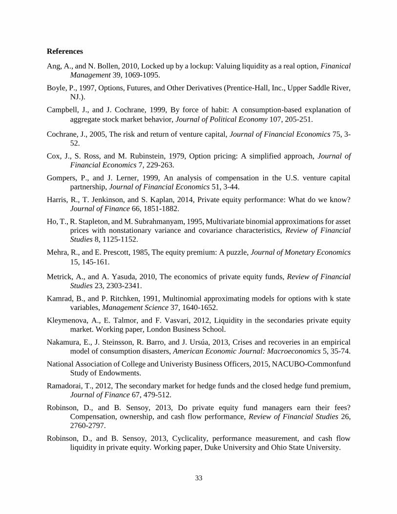
33
References
Ang, A., and N. Bollen, 2010, Locked up by a lockup: Valuing liquidity as a real option, Finanical
Management 39, 1069-1095.
Boyle, P., 1997, Options, Futures, and Other Derivatives (Prentice-Hall, Inc., Upper Saddle River,
NJ.).
Campbell, J., and J. Cochrane, 1999, By force of habit: A consumption-based explanation of
aggregate stock market behavior, Journal of Political Economy 107, 205-251.
Cochrane, J., 2005, The risk and return of venture capital, Journal of Financial Economics 75, 3-
52.
Cox, J., S. Ross, and M. Rubinstein, 1979, Option pricing: A simplified approach, Journal of
Financial Economics 7, 229-263.
Gompers, P., and J. Lerner, 1999, An analysis of compensation in the U.S. venture capital
partnership, Journal of Financial Economics 51, 3-44.
Harris, R., T. Jenkinson, and S. Kaplan, 2014, Private equity performance: What do we know?
Journal of Finance 66, 1851-1882.
Ho, T., R. Stapleton, and M. Subrahmanyam, 1995, Multivariate binomial approximations for asset
prices with nonstationary variance and covariance characteristics, Review of Financial
Studies 8, 1125-1152.
Mehra, R., and E. Prescott, 1985, The equity premium: A puzzle, Journal of Monetary Economics
15, 145-161.
Metrick, A., and A. Yasuda, 2010, The economics of private equity funds, Review of Financial
Studies 23, 2303-2341.
Kamrad, B., and P. Ritchken, 1991, Multinomial approximating models for options with k state
variables, Management Science 37, 1640-1652.
Kleymenova, A., E. Talmor, and F. Vasvari, 2012, Liquidity in the secondaries private equity
market. Working paper, London Business School.
Nakamura, E., J. Steinsson, R. Barro, and J. Ursúa, 2013, Crises and recoveries in an empirical
model of consumption disasters, American Economic Journal: Macroeconomics 5, 35-74.
National Association of College and Univeristy Business Officers, 2015, NACUBO-Commonfund
Study of Endowments.
Ramadorai, T., 2012, The secondary market for hedge funds and the closed hedge fund premium,
Journal of Finance 67, 479-512.
Robinson, D., and B. Sensoy, 2013, Do private equity fund managers earn their fees?
Compensation, ownership, and cash flow performance, Review of Financial Studies 26,
2760-2797.
Robinson, D., and B. Sensoy, 2013, Cyclicality, performance measurement, and cash flow
liquidity in private equity. Working paper, Duke University and Ohio State University.

34
Shliefer, A., and R. Vishny, 2011, Fire sales in finance and macroeconomics, Journal of Economic
Perspectives 25, 29-48.
Sorensen, M., N. Wang, and J. Yang, 2014, Valuing private equity, Review of Financial Studies
27, 1977-2021.
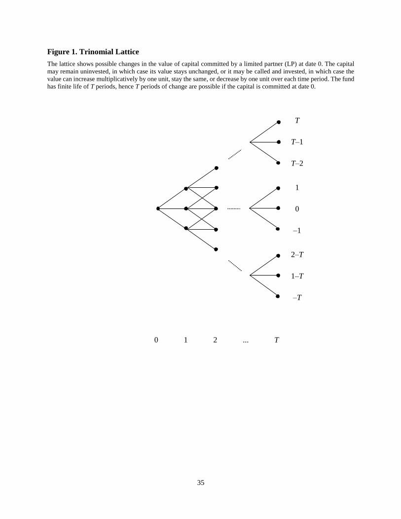
35
Figure 1. Trinomial Lattice
The lattice shows possible changes in the value of capital committed by a limited partner (LP) at date 0. The capital
may remain uninvested, in which case its value stays unchanged, or it may be called and invested, in which case the
value can increase multiplicatively by one unit, stay the same, or decrease by one unit over each time period. The fund
has finite life of T periods, hence T periods of change are possible if the capital is committed at date 0.
T
T–1
T–2
1
0
–1
2–T
1–T
–T
0 1 2 ... T
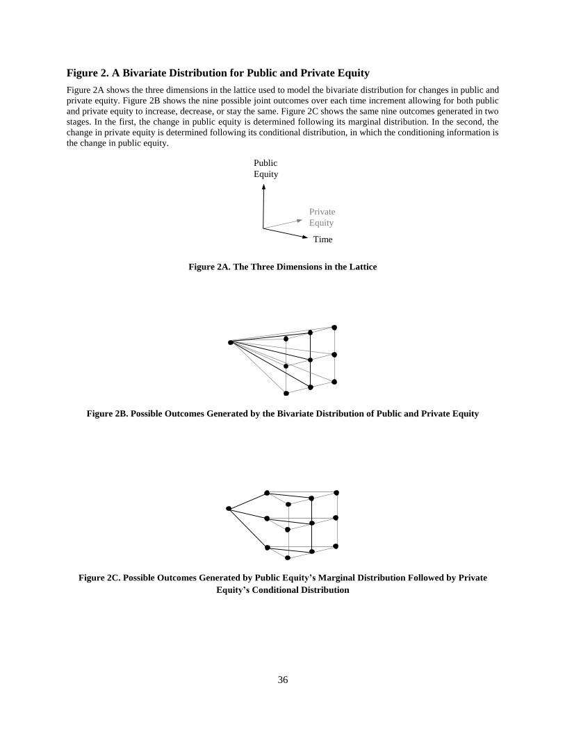
36
Figure 2. A Bivariate Distribution for Public and Private Equity
Figure 2A shows the three dimensions in the lattice used to model the bivariate distribution for changes in public and
private equity. Figure 2B shows the nine possible joint outcomes over each time increment allowing for both public
and private equity to increase, decrease, or stay the same. Figure 2C shows the same nine outcomes generated in two
stages. In the first, the change in public equity is determined following its marginal distribution. In the second, the
change in private equity is determined following its conditional distribution, in which the conditioning information is
the change in public equity.
Figure 2A. The Three Dimensions in the Lattice
Figure 2B. Possible Outcomes Generated by the Bivariate Distribution of Public and Private Equity
Figure 2C. Possible Outcomes Generated by Public Equity’s Marginal Distribution Followed by Private
Equity’s Conditional Distribution
Time
Public
Equity
Private
Equity
37
Figure 3. Probability of a Large Haircut
Depicted is the probability of a large haircut as a function of the cumulative number of net increases or decreases in
public equity values.
0%
10%
20%
30%
40%
50%
60%
70%
80%
90%
100%
-48 -36 -24 -12 0 12 24 36 48
Pro
bab
ilit
y o
f a
Lar
ge
Hai
rcut
Net Quarterly Changes in Public Equity
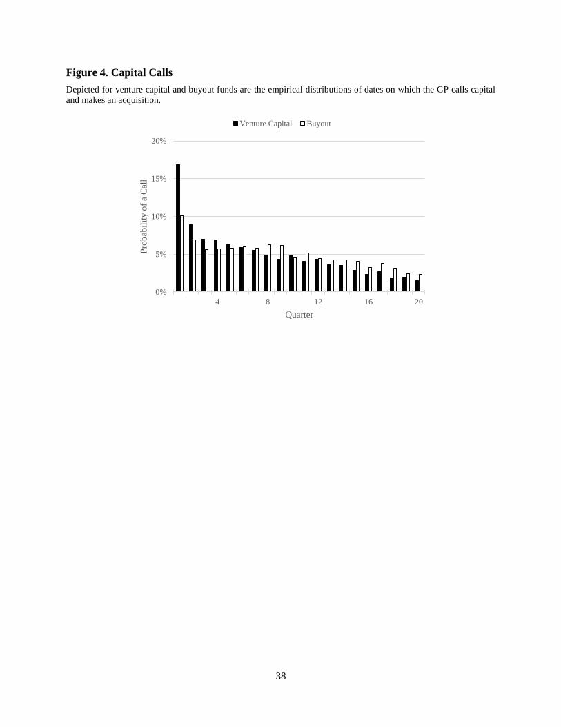
38
Figure 4. Capital Calls
Depicted for venture capital and buyout funds are the empirical distributions of dates on which the GP calls capital
and makes an acquisition.
0%
5%
10%
15%
20%
4 8 12 16 20
Pro
bab
ilit
y o
f a
Cal
l
Quarter
Venture Capital Buyout
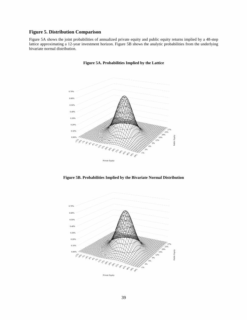
39
Figure 5. Distribution Comparison
Figure 5A shows the joint probabilities of annualized private equity and public equity returns implied by a 48-step
lattice approximating a 12-year investment horizon. Figure 5B shows the analytic probabilities from the underlying
bivariate normal distribution.
Figure 5A. Probabilities Implied by the Lattice
Figure 5B. Probabilities Implied by the Bivariate Normal Distribution
-1%
2%
6%
9%
12%
16%
20%
23%
27%
0.00%
0.10%
0.20%
0.30%
0.40%
0.50%
0.60%
0.70%
Pub
lic
Eq
uit
y
Private Equity
-1%
2%
6%
9%
12%
16%
20%
23%
27%
0.00%
0.10%
0.20%
0.30%
0.40%
0.50%
0.60%
0.70%
Pub
lic
Eq
uit
y
Private Equity
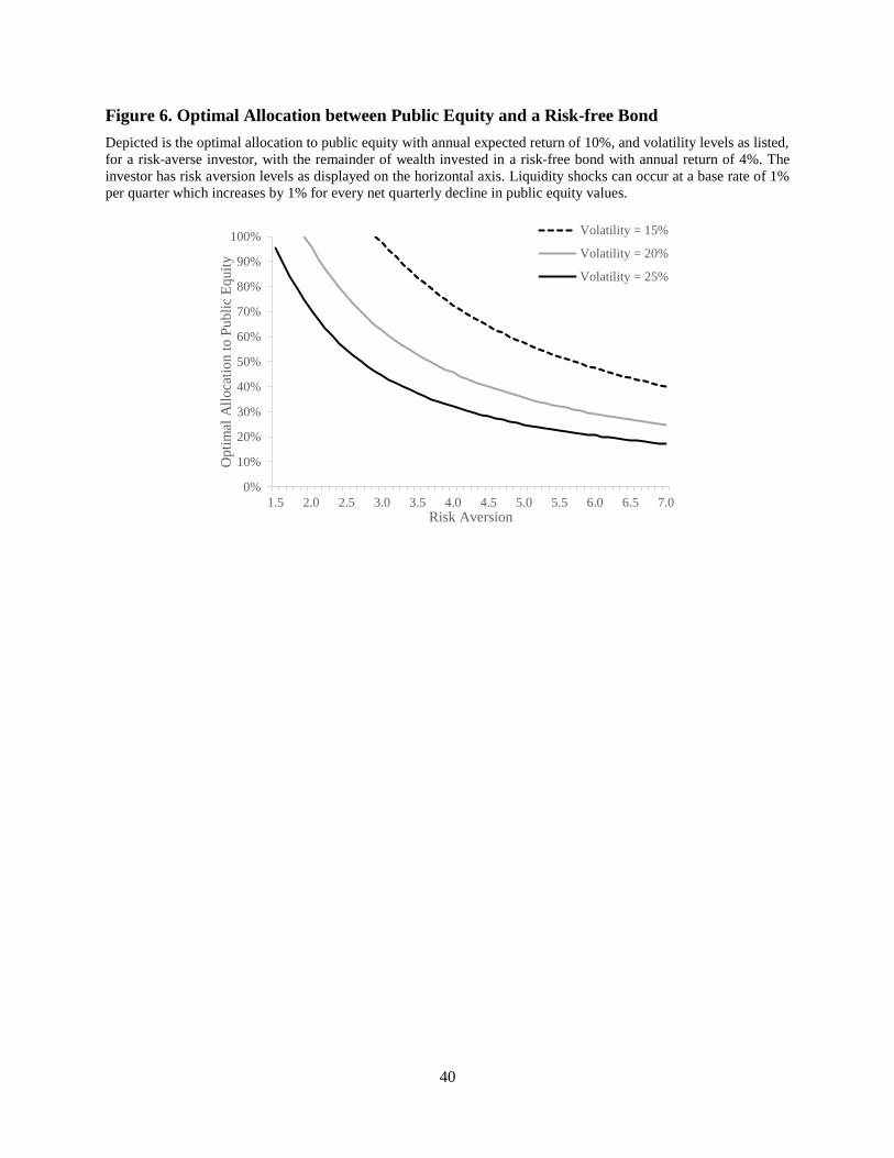
40
Figure 6. Optimal Allocation between Public Equity and a Risk-free Bond
Depicted is the optimal allocation to public equity with annual expected return of 10%, and volatility levels as listed,
for a risk-averse investor, with the remainder of wealth invested in a risk-free bond with annual return of 4%. The
investor has risk aversion levels as displayed on the horizontal axis. Liquidity shocks can occur at a base rate of 1%
per quarter which increases by 1% for every net quarterly decline in public equity values.
0%
10%
20%
30%
40%
50%
60%
70%
80%
90%
100%
1.5 2.0 2.5 3.0 3.5 4.0 4.5 5.0 5.5 6.0 6.5 7.0
Op
tim
al A
llo
cati
on t
o P
ub
lic
Eq
uit
y
Risk Aversion
Volatility = 15%
Volatility = 20%
Volatility = 25%
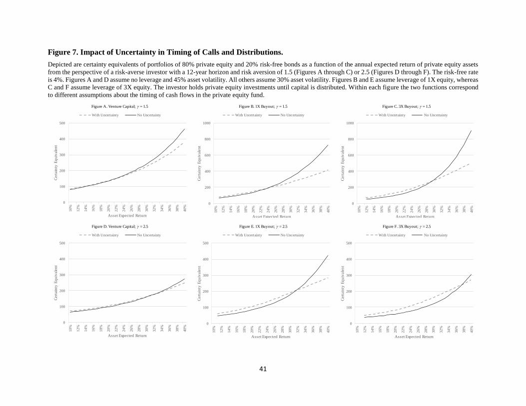
41
Figure 7. Impact of Uncertainty in Timing of Calls and Distributions.
Depicted are certainty equivalents of portfolios of 80% private equity and 20% risk-free bonds as a function of the annual expected return of private equity assets
from the perspective of a risk-averse investor with a 12-year horizon and risk aversion of 1.5 (Figures A through C) or 2.5 (Figures D through F). The risk-free rate
is 4%. Figures A and D assume no leverage and 45% asset volatility. All others assume 30% asset volatility. Figures B and E assume leverage of 1X equity, whereas
C and F assume leverage of 3X equity. The investor holds private equity investments until capital is distributed. Within each figure the two functions correspond
to different assumptions about the timing of cash flows in the private equity fund.
Figure A. Venture Capital; = 1.5 Figure B. 1X Buyout; = 1.5 Figure C. 3X Buyout; = 1.5
0
100
200
300
400
500
10%
12%
14%
16%
18%
20%
22%
24%
26%
28%
30%
32%
34%
36%
38%
40%
Cert
ain
ty E
qu
ivale
nt
Asset Expected Return
With Uncertainty No Uncertainty
0
200
400
600
800
1000
10
%
12
%
14
%
16
%
18
%
20
%
22
%
24
%
26
%
28
%
30
%
32
%
34
%
36
%
38
%
40
%
Cert
ain
ty E
qu
ivale
nt
Asset Expected Return
With Uncertainty No Uncertainty
0
200
400
600
800
1000
10
%
12
%
14
%
16
%
18
%
20
%
22
%
24
%
26
%
28
%
30
%
32
%
34
%
36
%
38
%
40
%
Cert
ain
ty E
qu
ivale
nt
Asset Expected Return
With Uncertainty No Uncertainty
Figure D. Venture Capital; = 2.5 Figure E. 1X Buyout; = 2.5 Figure F. 3X Buyout; = 2.5
0
100
200
300
400
500
10
%
12
%
14
%
16
%
18
%
20
%
22
%
24
%
26
%
28
%
30
%
32
%
34
%
36
%
38
%
40
%
Cert
ain
ty E
qu
ivale
nt
Asset Expected Return
With Uncertainty No Uncertainty
0
100
200
300
400
500
10
%
12
%
14
%
16
%
18
%
20
%
22
%
24
%
26
%
28
%
30
%
32
%
34
%
36
%
38
%
40
%
Cert
ain
ty E
qu
ivale
nt
Asset Expected Return
With Uncertainty No Uncertainty
0
100
200
300
400
500
10
%
12
%
14
%
16
%
18
%
20
%
22
%
24
%
26
%
28
%
30
%
32
%
34
%
36
%
38
%
40
%
Cert
ain
ty E
qu
ivale
nt
Asset Expected Return
With Uncertainty No Uncertainty
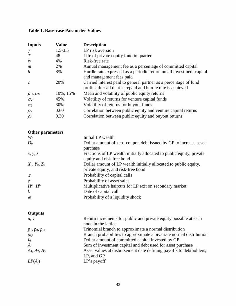
42
Table 1. Base-case Parameter Values
Inputs Value Description
1.5-3.5 LP risk aversion
T 48 Life of private equity fund in quarters
rf 4% Risk-free rate
m 2% Annual management fee as a percentage of committed capital
h 8% Hurdle rate expressed as a periodic return on all investment capital
and management fees paid
c 20% Carried interest paid to general partner as a percentage of fund
profits after all debt is repaid and hurdle rate is achieved
U, U 10%, 15% Mean and volatility of public equity returns
V 45% Volatility of returns for venture capital funds
B 30% Volatility of returns for buyout funds
V 0.60 Correlation between public equity and venture capital returns
B 0.30 Correlation between public equity and buyout returns
Other parameters
W0 Initial LP wealth
D0 Dollar amount of zero-coupon debt issued by GP to increase asset
purchase
x, y, z Fractions of LP wealth initially allocated to public equity, private
equity and risk-free bond
X0, Y0, Z0 Dollar amount of LP wealth initially allocated to public equity,
private equity, and risk-free bond
Probability of capital calls
Probability of asset sales
HH, HL Multiplicative haircuts for LP exit on secondary market
k Date of capital call
Probability of a liquidity shock
Outputs
u, v Return increments for public and private equity possible at each
node in the lattice
p1, p0, p-1 Trinomial branch to approximate a normal distribution
pi,j Branch probabilities to approximate a bivariate normal distribution
I0 Dollar amount of committed capital invested by GP
A0 Sum of investment capital and debt used for asset purchase
A1, A2, A3 Asset values at disbursement date defining payoffs to debtholders,
LP, and GP
LP(At) LP’s payoff
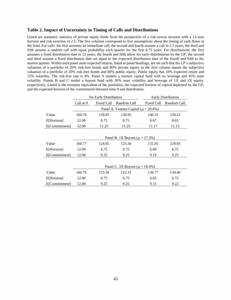
43
Table 2. Impact of Uncertainty in Timing of Calls and Distributions
Listed are summary statistics of private equity funds from the perspective of a risk-averse investor with a 12-year
horizon and risk aversion of 2.5. The five columns correspond to five assumptions about the timing of cash flows in
the fund. For calls: the first assumes an immediate call; the second and fourth assume a call in 2.5 years; the third and
fifth assume a random call with equal probability each quarter for the first 4.75 years. For distributions: the first
assumes a fixed distribution date in 12 years; the fourth and fifth allow for early distributions by the GP; the second
and third assume a fixed distribution date set equal to the expected distribution date of the fourth and fifth to the
nearest quarter. Within each panel asset expected returns, listed in panel headings, are set such that the LP’s subjective
valuation of a portfolio of 20% risk-free bonds and 80% private equity in the first column equals the subjective
valuation of a portfolio of 20% risk-free bonds and 80% public equity. Public equity has 10% expected return and
15% volatility. The risk-free rate is 4%. Panel A models a venture capital fund with no leverage and 45% asset
volatility. Panels B and C model a buyout fund with 30% asset volatility and leverage of 1X and 3X equity,
respectively. Listed is the certainty equivalent of the portfolios, the expected horizon of capital deployed by the GP,
and the expected horizon of the commitment between time 0 and distribution.
No Early Distribution Early Distribution
Call at 0 Fixed Call Random Call Fixed Call Random Call
Panel A. Venture Capital ( = 20.6%)
Value 160.76 139.83 138.95 140.31 139.22
E[Horizon] 12.00 8.75 8.75 8.67 8.65
E[Commitment] 12.00 11.25 11.25 11.17 11.15
Panel B. 1X Buyout ( = 17.3%)
Value 160.77 124.65 123.56 131.05 129.83
E[Horizon] 12.00 6.75 6.75 6.69 6.75
E[Commitment] 12.00 9.25 9.25 9.19 9.25
Panel C. 3X Buyout ( = 18.4%)
Value 160.76 123.36 122.31 136.77 134.40
E[Horizon] 12.00 6.75 6.75 6.65 6.72
E[Commitment] 12.00 9.25 9.25 9.15 9.22
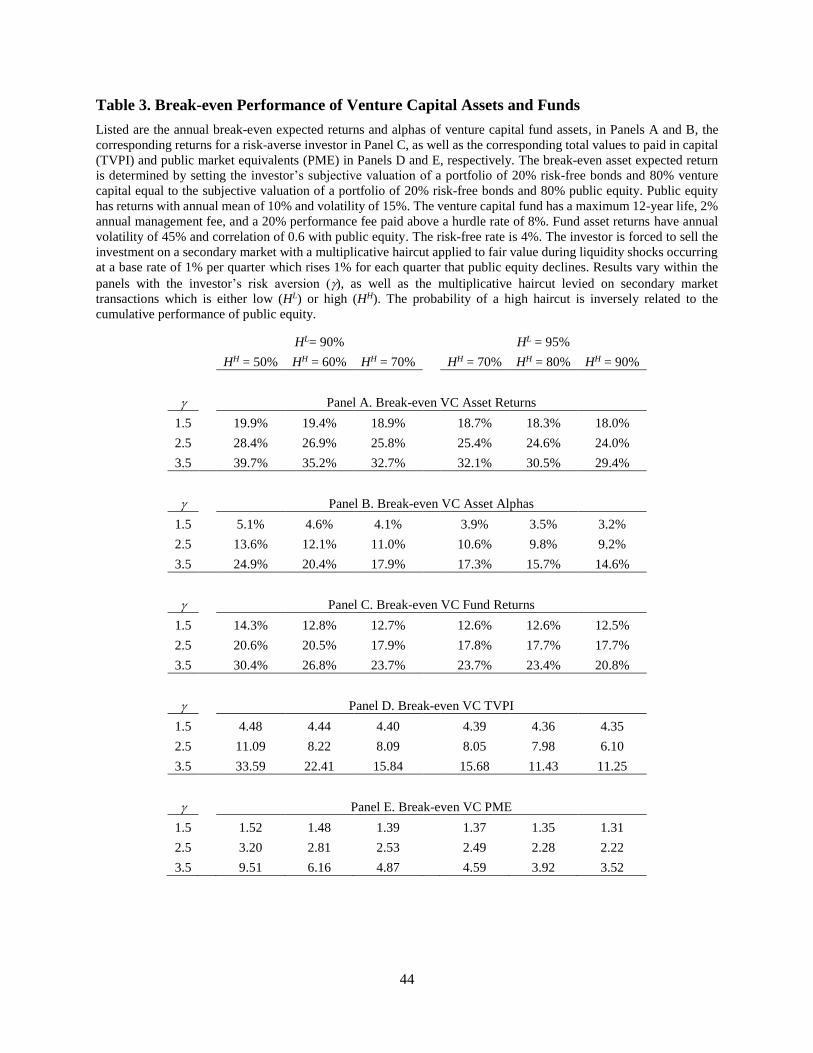
44
Table 3. Break-even Performance of Venture Capital Assets and Funds
Listed are the annual break-even expected returns and alphas of venture capital fund assets, in Panels A and B, the
corresponding returns for a risk-averse investor in Panel C, as well as the corresponding total values to paid in capital
(TVPI) and public market equivalents (PME) in Panels D and E, respectively. The break-even asset expected return
is determined by setting the investor’s subjective valuation of a portfolio of 20% risk-free bonds and 80% venture
capital equal to the subjective valuation of a portfolio of 20% risk-free bonds and 80% public equity. Public equity
has returns with annual mean of 10% and volatility of 15%. The venture capital fund has a maximum 12-year life, 2%
annual management fee, and a 20% performance fee paid above a hurdle rate of 8%. Fund asset returns have annual
volatility of 45% and correlation of 0.6 with public equity. The risk-free rate is 4%. The investor is forced to sell the
investment on a secondary market with a multiplicative haircut applied to fair value during liquidity shocks occurring
at a base rate of 1% per quarter which rises 1% for each quarter that public equity declines. Results vary within the
panels with the investor’s risk aversion (), as well as the multiplicative haircut levied on secondary market
transactions which is either low (HL) or high (HH). The probability of a high haircut is inversely related to the
cumulative performance of public equity.
HL= 90% HL = 95%
HH = 50% HH = 60% HH = 70% HH = 70% HH = 80% HH = 90%
Panel A. Break-even VC Asset Returns
1.5 19.9% 19.4% 18.9% 18.7% 18.3% 18.0%
2.5 28.4% 26.9% 25.8% 25.4% 24.6% 24.0%
3.5 39.7% 35.2% 32.7% 32.1% 30.5% 29.4%
Panel B. Break-even VC Asset Alphas
1.5 5.1% 4.6% 4.1% 3.9% 3.5% 3.2%
2.5 13.6% 12.1% 11.0% 10.6% 9.8% 9.2%
3.5 24.9% 20.4% 17.9% 17.3% 15.7% 14.6%
Panel C. Break-even VC Fund Returns
1.5 14.3% 12.8% 12.7% 12.6% 12.6% 12.5%
2.5 20.6% 20.5% 17.9% 17.8% 17.7% 17.7%
3.5 30.4% 26.8% 23.7% 23.7% 23.4% 20.8%
Panel D. Break-even VC TVPI
1.5 4.48 4.44 4.40 4.39 4.36 4.35
2.5 11.09 8.22 8.09 8.05 7.98 6.10
3.5 33.59 22.41 15.84 15.68 11.43 11.25
Panel E. Break-even VC PME
1.5 1.52 1.48 1.39 1.37 1.35 1.31
2.5 3.20 2.81 2.53 2.49 2.28 2.22
3.5 9.51 6.16 4.87 4.59 3.92 3.52

45
Table 4. Break-even Performance of 1X Buyout Assets and Funds
Listed are the annual break-even expected returns and alphas of buyout fund assets, in Panels A and B, the
corresponding returns for a risk-averse investor in Panel C, as well as the corresponding total values to paid in capital
(TVPI) and public market equivalents (PME) in Panels D and E, respectively. The break-even asset expected return
is determined by setting the investor’s subjective valuation of a portfolio of 20% risk-free bonds and 80% buyout fund
equal to the subjective valuation of a portfolio of 20% risk-free bonds and 80% public equity. Public equity has returns
with annual mean of 10% and volatility of 15%. The buyout fund has a maximum 12-year life, 1X leverage, 2% annual
management fee, and a 20% performance fee paid above a hurdle rate of 8%. Fund asset returns have annual volatility
of 30% and correlation of 0.3 with public equity. The risk-free rate is 4%. The investor is forced to sell the investment
on a secondary market with a multiplicative haircut applied to fair value during liquidity shocks occurring at a base
rate of 1% per quarter which rises 1% for each quarter that public equity declines. Results vary within the panels with
the investor’s risk aversion (), as well as the multiplicative haircut levied on secondary market transactions which is
either low (HL) or high (HH). The probability of a high haircut is inversely related to the cumulative performance of
public equity.
HL= 90% HL = 95%
HH = 50% HH = 60% HH = 70% HH = 70% HH = 80% HH = 90%
Panel A. Break-even 1X Buyout Asset Returns
1.5 17.7% 17.3% 16.9% 16.8% 16.5% 16.2%
2.5 23.6% 22.5% 21.8% 21.5% 21.0% 20.6%
3.5 32.0% 29.1% 27.5% 27.1% 26.1% 25.5%
Panel B. Break-even 1X Buyout Asset Alphas
1.5 10.1% 9.7% 9.3% 9.2% 8.9% 8.6%
2.5 16.0% 14.9% 14.2% 13.9% 13.4% 13.0%
3.5 24.4% 21.5% 19.9% 19.5% 18.5% 17.9%
Panel C. Break-even 1X Buyout Fund Returns
1.5 16.0% 15.7% 15.2% 15.0% 14.7% 14.4%
2.5 20.5% 19.7% 18.9% 18.6% 18.4% 18.2%
3.5 27.6% 25.1% 23.4% 23.0% 22.7% 22.2%
Panel D. Break-even 1X Buyout TVPI
1.5 3.88 3.79 3.73 3.72 3.67 3.62
2.5 5.96 5.74 5.55 5.47 4.81 4.74
3.5 10.58 9.65 7.82 7.73 7.48 7.31
Panel E. Break-even 1X Buyout PME
1.5 1.61 1.57 1.54 1.53 1.50 1.46
2.5 2.41 2.23 2.14 2.09 2.01 1.97
3.5 4.39 3.55 3.16 3.07 2.86 2.75
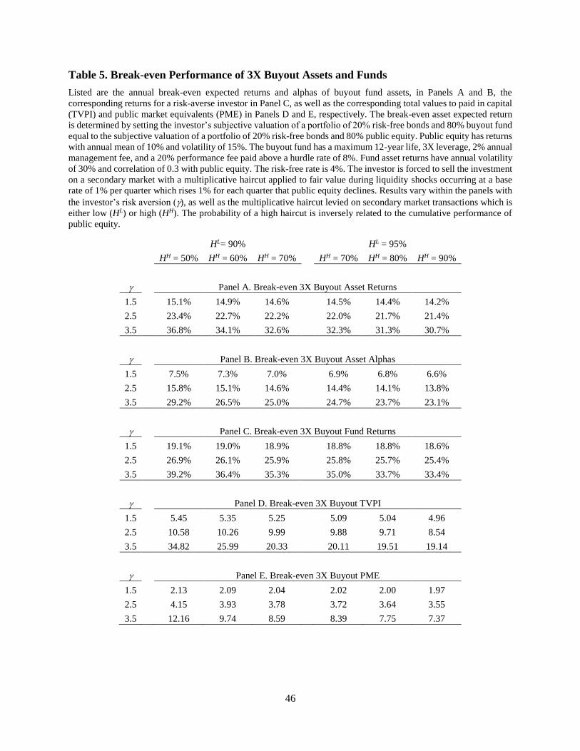
46
Table 5. Break-even Performance of 3X Buyout Assets and Funds
Listed are the annual break-even expected returns and alphas of buyout fund assets, in Panels A and B, the
corresponding returns for a risk-averse investor in Panel C, as well as the corresponding total values to paid in capital
(TVPI) and public market equivalents (PME) in Panels D and E, respectively. The break-even asset expected return
is determined by setting the investor’s subjective valuation of a portfolio of 20% risk-free bonds and 80% buyout fund
equal to the subjective valuation of a portfolio of 20% risk-free bonds and 80% public equity. Public equity has returns
with annual mean of 10% and volatility of 15%. The buyout fund has a maximum 12-year life, 3X leverage, 2% annual
management fee, and a 20% performance fee paid above a hurdle rate of 8%. Fund asset returns have annual volatility
of 30% and correlation of 0.3 with public equity. The risk-free rate is 4%. The investor is forced to sell the investment
on a secondary market with a multiplicative haircut applied to fair value during liquidity shocks occurring at a base
rate of 1% per quarter which rises 1% for each quarter that public equity declines. Results vary within the panels with
the investor’s risk aversion (), as well as the multiplicative haircut levied on secondary market transactions which is
either low (HL) or high (HH). The probability of a high haircut is inversely related to the cumulative performance of
public equity.
HL= 90% HL = 95%
HH = 50% HH = 60% HH = 70% HH = 70% HH = 80% HH = 90%
Panel A. Break-even 3X Buyout Asset Returns
1.5 15.1% 14.9% 14.6% 14.5% 14.4% 14.2%
2.5 23.4% 22.7% 22.2% 22.0% 21.7% 21.4%
3.5 36.8% 34.1% 32.6% 32.3% 31.3% 30.7%
Panel B. Break-even 3X Buyout Asset Alphas
1.5 7.5% 7.3% 7.0% 6.9% 6.8% 6.6%
2.5 15.8% 15.1% 14.6% 14.4% 14.1% 13.8%
3.5 29.2% 26.5% 25.0% 24.7% 23.7% 23.1%
Panel C. Break-even 3X Buyout Fund Returns
1.5 19.1% 19.0% 18.9% 18.8% 18.8% 18.6%
2.5 26.9% 26.1% 25.9% 25.8% 25.7% 25.4%
3.5 39.2% 36.4% 35.3% 35.0% 33.7% 33.4%
Panel D. Break-even 3X Buyout TVPI
1.5 5.45 5.35 5.25 5.09 5.04 4.96
2.5 10.58 10.26 9.99 9.88 9.71 8.54
3.5 34.82 25.99 20.33 20.11 19.51 19.14
Panel E. Break-even 3X Buyout PME
1.5 2.13 2.09 2.04 2.02 2.00 1.97
2.5 4.15 3.93 3.78 3.72 3.64 3.55
3.5 12.16 9.74 8.59 8.39 7.75 7.37
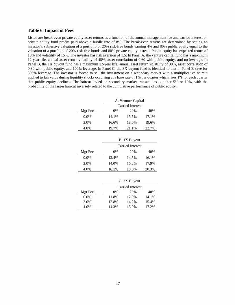
47
Table 6. Impact of Fees
Listed are break-even private equity asset returns as a function of the annual management fee and carried interest on
private equity fund profits paid above a hurdle rate of 8%. The break-even returns are determined by setting an
investor’s subjective valuation of a portfolio of 20% risk-free bonds earning 4% and 80% public equity equal to the
valuation of a portfolio of 20% risk-free bonds and 80% private equity instead. Public equity has expected return of
10% and volatility of 15%. The investor has risk aversion of 1.5. In Panel A, the venture capital fund has a maximum
12-year life, annual asset return volatility of 45%, asset correlation of 0.60 with public equity, and no leverage. In
Panel B, the 1X buyout fund has a maximum 12-year life, annual asset return volatility of 30%, asset correlation of
0.30 with public equity, and 100% leverage. In Panel C, the 3X buyout fund is identical to that in Panel B save for
300% leverage. The investor is forced to sell the investment on a secondary market with a multiplicative haircut
applied to fair value during liquidity shocks occurring at a base rate of 1% per quarter which rises 1% for each quarter
that public equity declines. The haircut levied on secondary market transactions is either 5% or 10%, with the
probability of the larger haircut inversely related to the cumulative performance of public equity.
A. Venture Capital
Carried Interest
Mgt Fee 0% 20% 40%
0.0% 14.1% 15.5% 17.1%
2.0% 16.6% 18.0% 19.6%
4.0% 19.7% 21.1% 22.7%
B. 1X Buyout
Carried Interest
Mgt Fee 0% 20% 40%
0.0% 12.4% 14.5% 16.1%
2.0% 14.0% 16.2% 17.9%
4.0% 16.1% 18.6% 20.3%
C. 3X Buyout
Carried Interest
Mgt Fee 0% 20% 40%
0.0% 11.8% 12.9% 14.1%
2.0% 12.8% 14.2% 15.4%
4.0% 14.3% 15.9% 17.2%
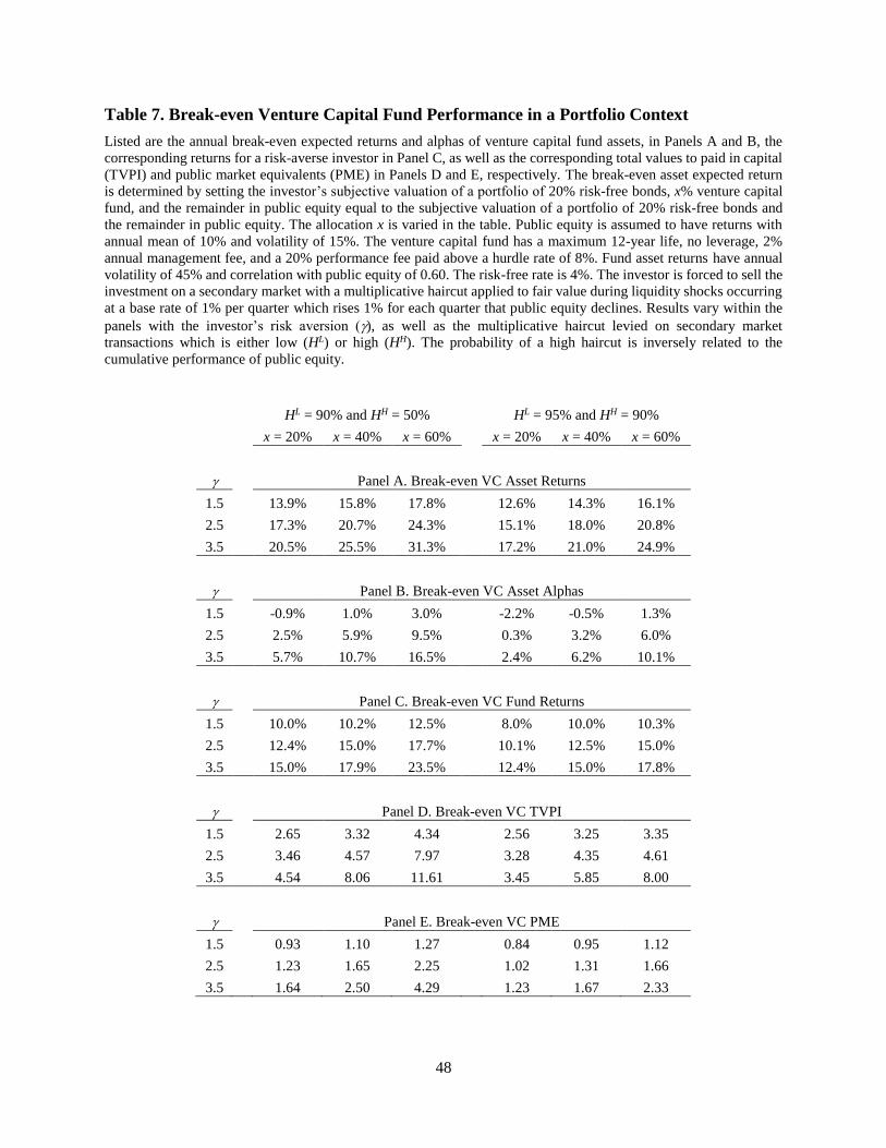
48
Table 7. Break-even Venture Capital Fund Performance in a Portfolio Context
Listed are the annual break-even expected returns and alphas of venture capital fund assets, in Panels A and B, the
corresponding returns for a risk-averse investor in Panel C, as well as the corresponding total values to paid in capital
(TVPI) and public market equivalents (PME) in Panels D and E, respectively. The break-even asset expected return
is determined by setting the investor’s subjective valuation of a portfolio of 20% risk-free bonds, x% venture capital
fund, and the remainder in public equity equal to the subjective valuation of a portfolio of 20% risk-free bonds and
the remainder in public equity. The allocation x is varied in the table. Public equity is assumed to have returns with
annual mean of 10% and volatility of 15%. The venture capital fund has a maximum 12-year life, no leverage, 2%
annual management fee, and a 20% performance fee paid above a hurdle rate of 8%. Fund asset returns have annual
volatility of 45% and correlation with public equity of 0.60. The risk-free rate is 4%. The investor is forced to sell the
investment on a secondary market with a multiplicative haircut applied to fair value during liquidity shocks occurring
at a base rate of 1% per quarter which rises 1% for each quarter that public equity declines. Results vary within the
panels with the investor’s risk aversion (), as well as the multiplicative haircut levied on secondary market
transactions which is either low (HL) or high (HH). The probability of a high haircut is inversely related to the
cumulative performance of public equity.
HL = 90% and HH = 50% HL = 95% and HH = 90%
x = 20% x = 40% x = 60% x = 20% x = 40% x = 60%
Panel A. Break-even VC Asset Returns
1.5 13.9% 15.8% 17.8% 12.6% 14.3% 16.1%
2.5 17.3% 20.7% 24.3% 15.1% 18.0% 20.8%
3.5 20.5% 25.5% 31.3% 17.2% 21.0% 24.9%
Panel B. Break-even VC Asset Alphas
1.5 -0.9% 1.0% 3.0% -2.2% -0.5% 1.3%
2.5 2.5% 5.9% 9.5% 0.3% 3.2% 6.0%
3.5 5.7% 10.7% 16.5% 2.4% 6.2% 10.1%
Panel C. Break-even VC Fund Returns
1.5 10.0% 10.2% 12.5% 8.0% 10.0% 10.3%
2.5 12.4% 15.0% 17.7% 10.1% 12.5% 15.0%
3.5 15.0% 17.9% 23.5% 12.4% 15.0% 17.8%
Panel D. Break-even VC TVPI
1.5 2.65 3.32 4.34 2.56 3.25 3.35
2.5 3.46 4.57 7.97 3.28 4.35 4.61
3.5 4.54 8.06 11.61 3.45 5.85 8.00
Panel E. Break-even VC PME
1.5 0.93 1.10 1.27 0.84 0.95 1.12
2.5 1.23 1.65 2.25 1.02 1.31 1.66
3.5 1.64 2.50 4.29 1.23 1.67 2.33
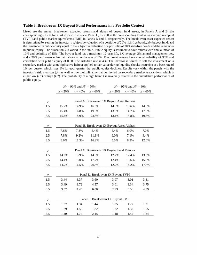
49
Table 8. Break-even 1X Buyout Fund Performance in a Portfolio Context
Listed are the annual break-even expected returns and alphas of buyout fund assets, in Panels A and B, the
corresponding returns for a risk-averse investor in Panel C, as well as the corresponding total values to paid in capital
(TVPI) and public market equivalents (PME) in Panels D and E, respectively. The break-even asset expected return
is determined by setting the investor’s subjective valuation of a portfolio of 20% risk-free bonds, x% buyout fund, and
the remainder in public equity equal to the subjective valuation of a portfolio of 20% risk-free bonds and the remainder
in public equity. The allocation x is varied in the table. Public equity is assumed to have returns with annual mean of
10% and volatility of 15%. The buyout fund has a maximum 12-year life, 1X leverage, 2% annual management fee,
and a 20% performance fee paid above a hurdle rate of 8%. Fund asset returns have annual volatility of 30% and
correlation with public equity of 0.30. The risk-free rate is 4%. The investor is forced to sell the investment on a
secondary market with a multiplicative haircut applied to fair value during liquidity shocks occurring at a base rate of
1% per quarter which rises 1% for each quarter that public equity declines. Results vary within the panels with the
investor’s risk aversion (), as well as the multiplicative haircut levied on secondary market transactions which is
either low (HL) or high (HH). The probability of a high haircut is inversely related to the cumulative performance of
public equity.
HL = 90% and HH = 50% HL = 95% and HH = 90%
x = 20% x = 40% x = 60% x = 20% x = 40% x = 60%
Panel A. Break-even 1X Buyout Asset Returns
1.5 15.2% 14.9% 16.0% 14.0% 13.6% 14.6%
2.5 15.4% 16.8% 19.5% 13.6% 14.7% 17.0%
3.5 15.6% 18.9% 23.8% 13.1% 15.8% 19.6%
Panel B. Break-even 1X Buyout Asset Alphas
1.5 7.6% 7.3% 8.4% 6.4% 6.0% 7.0%
2.5 7.8% 9.2% 11.9% 6.0% 7.1% 9.4%
3.5 8.0% 11.3% 16.2% 5.5% 8.2% 12.0%
Panel C. Break-even 1X Buyout Fund Returns
1.5 14.0% 13.9% 14.3% 12.7% 12.4% 13.5%
2.5 14.1% 15.0% 17.2% 12.4% 13.6% 15.3%
3.5 14.2% 16.5% 20.5% 12.2% 14.2% 17.3%
Panel D. Break-even 1X Buyout TVPI
1.5 3.44 3.37 3.60 3.07 3.01 3.31
2.5 3.49 3.72 4.57 3.01 3.34 3.75
3.5 3.52 4.45 6.00 2.93 3.56 4.59
Panel E. Break-even 1X Buyout PME
1.5 1.37 1.34 1.44 1.25 1.22 1.31
2.5 1.39 1.53 1.82 1.22 1.32 1.55
3.5 1.40 1.75 2.45 1.18 1.42 1.84
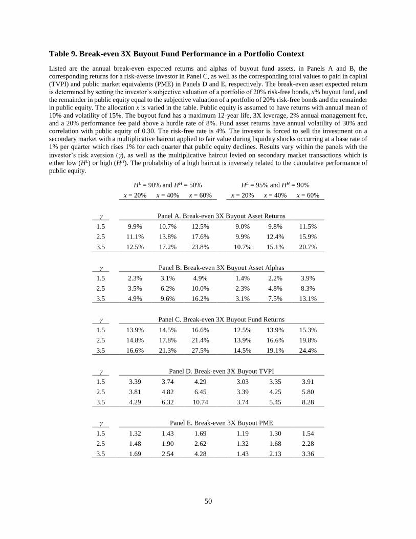
50
Table 9. Break-even 3X Buyout Fund Performance in a Portfolio Context
Listed are the annual break-even expected returns and alphas of buyout fund assets, in Panels A and B, the
corresponding returns for a risk-averse investor in Panel C, as well as the corresponding total values to paid in capital
(TVPI) and public market equivalents (PME) in Panels D and E, respectively. The break-even asset expected return
is determined by setting the investor’s subjective valuation of a portfolio of 20% risk-free bonds, x% buyout fund, and
the remainder in public equity equal to the subjective valuation of a portfolio of 20% risk-free bonds and the remainder
in public equity. The allocation x is varied in the table. Public equity is assumed to have returns with annual mean of
10% and volatility of 15%. The buyout fund has a maximum 12-year life, 3X leverage, 2% annual management fee,
and a 20% performance fee paid above a hurdle rate of 8%. Fund asset returns have annual volatility of 30% and
correlation with public equity of 0.30. The risk-free rate is 4%. The investor is forced to sell the investment on a
secondary market with a multiplicative haircut applied to fair value during liquidity shocks occurring at a base rate of
1% per quarter which rises 1% for each quarter that public equity declines. Results vary within the panels with the
investor’s risk aversion (), as well as the multiplicative haircut levied on secondary market transactions which is
either low (HL) or high (HH). The probability of a high haircut is inversely related to the cumulative performance of
public equity.
HL = 90% and HH = 50% HL = 95% and HH = 90%
x = 20% x = 40% x = 60% x = 20% x = 40% x = 60%
Panel A. Break-even 3X Buyout Asset Returns
1.5 9.9% 10.7% 12.5% 9.0% 9.8% 11.5%
2.5 11.1% 13.8% 17.6% 9.9% 12.4% 15.9%
3.5 12.5% 17.2% 23.8% 10.7% 15.1% 20.7%
Panel B. Break-even 3X Buyout Asset Alphas
1.5 2.3% 3.1% 4.9% 1.4% 2.2% 3.9%
2.5 3.5% 6.2% 10.0% 2.3% 4.8% 8.3%
3.5 4.9% 9.6% 16.2% 3.1% 7.5% 13.1%
Panel C. Break-even 3X Buyout Fund Returns
1.5 13.9% 14.5% 16.6% 12.5% 13.9% 15.3%
2.5 14.8% 17.8% 21.4% 13.9% 16.6% 19.8%
3.5 16.6% 21.3% 27.5% 14.5% 19.1% 24.4%
Panel D. Break-even 3X Buyout TVPI
1.5 3.39 3.74 4.29 3.03 3.35 3.91
2.5 3.81 4.82 6.45 3.39 4.25 5.80
3.5 4.29 6.32 10.74 3.74 5.45 8.28
Panel E. Break-even 3X Buyout PME
1.5 1.32 1.43 1.69 1.19 1.30 1.54
2.5 1.48 1.90 2.62 1.32 1.68 2.28
3.5 1.69 2.54 4.28 1.43 2.13 3.36
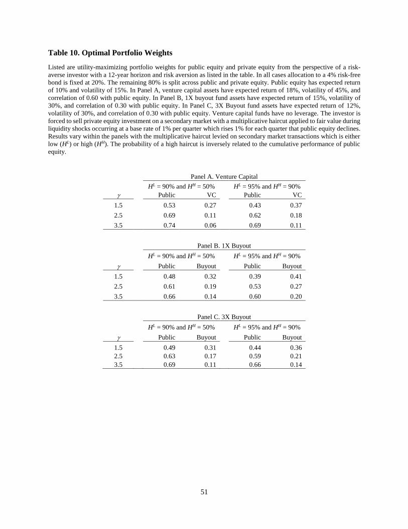
51
Table 10. Optimal Portfolio Weights
Listed are utility-maximizing portfolio weights for public equity and private equity from the perspective of a risk-
averse investor with a 12-year horizon and risk aversion as listed in the table. In all cases allocation to a 4% risk-free
bond is fixed at 20%. The remaining 80% is split across public and private equity. Public equity has expected return
of 10% and volatility of 15%. In Panel A, venture capital assets have expected return of 18%, volatility of 45%, and
correlation of 0.60 with public equity. In Panel B, 1X buyout fund assets have expected return of 15%, volatility of
30%, and correlation of 0.30 with public equity. In Panel C, 3X Buyout fund assets have expected return of 12%,
volatility of 30%, and correlation of 0.30 with public equity. Venture capital funds have no leverage. The investor is
forced to sell private equity investment on a secondary market with a multiplicative haircut applied to fair value during
liquidity shocks occurring at a base rate of 1% per quarter which rises 1% for each quarter that public equity declines.
Results vary within the panels with the multiplicative haircut levied on secondary market transactions which is either
low (HL) or high (HH). The probability of a high haircut is inversely related to the cumulative performance of public
equity.
Panel A. Venture Capital
HL = 90% and HH = 50% HL = 95% and HH = 90%
Public VC Public VC
1.5 0.53 0.27 0.43 0.37
2.5 0.69 0.11 0.62 0.18
3.5 0.74 0.06 0.69 0.11
Panel B. 1X Buyout
HL = 90% and HH = 50% HL = 95% and HH = 90%
Public Buyout Public Buyout
1.5 0.48 0.32 0.39 0.41
2.5 0.61 0.19 0.53 0.27
3.5 0.66 0.14 0.60 0.20
Panel C. 3X Buyout
HL = 90% and HH = 50% HL = 95% and HH = 90%
Public Buyout Public Buyout
1.5 0.49 0.31 0.44 0.36
2.5 0.63 0.17 0.59 0.21
3.5 0.69 0.11 0.66 0.14