Embed Size (px)
Citation preview

How the European day-ahead electricity market works
ELEC0018-1 - Marché de l'énergie - Pr. D. Ernst
Bertrand Cornélusse, Ph.D.
March 2017
1

Starting question
How is electrical energy traded in Europe?
2

Organization of the electrical power system (simplified)
Generation Companies
Generate electricity, provide balancing services,…
Large consumers
Buy electricity from producers, sell electricity to end-users
System Operators
Ensure reliability and security of the electrical network
Operates the electricity markets: facilitates energy trading and allocates cross-border capacity
Market Operators
Retailers
Buy electricity from producers, Generate their own electricity, sell their extra generation
3
OTC
OTC

Previous organization (simplified)
Generation Companies
ConsumersGenerate electricity, provide balancing services,…
Ensure reliability and security of the electrical network
Sell electricity to end-users
4

Why an Electricity Market?
Break monopolies and open electricity generation and retail to competition.
Facilitate exchanges between countries. This does not only require creating a markets in each country, but also coupling those markets.
Give incentives for building capacity/consuming electricity where appropriate. Market results provide time series of prices per area and period of the day, volumes that are exchanged, etc. This is part of necessary information to determine the appropriate capacity investments (at least in principle…).
5

What is an Electricity Market?
A centralized platform where participants can exchange electricity transparently according to the price they are will to pay or receive, and according to the capacity of the electrical network.
Fixed gate auction
• Participants submit sell or buy orders for several areas, several hours,
• the submissions are closed at a pre-specified time (closure)
• the market is cleared. Uniform clearing price: market prices are (well, should be ...) sufficient to determine whether orders are accepted or rejected
• Example: day-ahead. This is the topic of this lecture.
Continuous time auction
• Participants continuously submit orders. Orders are stored,
• Each time a deal is feasible, it is executed,
• Example: intra-day.
6

Markets by time horizon and activity
Intra-dayFutures
Towards real-time
BalancingDay-ahead
7

Markets by time horizon and activity
Intra-dayFutures
Towards real-time
BalancingDay-ahead
• Generation companies/retailers submit supply/demand orders
• TSOs allocate cross-border capacity
• Cleared once per day around 1PM
7

Day-ahead market operation and coupling
Each zone (or bidding area) has its own Power eXchange (PX) which collects participants orders.
France and Germany : EPEX spot, Belgium and the Netherlands: APX-Endex, etc.
Market coupling
• Perform clearing once per day for all coupled zones
• hence orders can be matched between markets
• and cross-border capacity is thus implicitly allocated.
• A price difference between countries must be explained by the congestion of some transmission lines.
Note: before market coupling, cross-border (i.e. inter-market) capacities were allocated through explicit auctions before deals were actually performed.
Detail: in general, each PX is responsible for the allocation to its participants (portfolio allocation). It has its own tie rules to lift indeterminacies.
8

Market operators / Power exchanges
9

History of the coupling project
10
COSMOS 2010
PCR 2014
GME 2015
4MMC 2015
Possible future extensions

0
150000
300000
450000
600000
Ger
man
yFr
ance UK
Italy
Spai
nTu
rkey
Swed
enPo
land
Nor
way
Net
herla
nds
Belg
ium
Finl
and
Aust
riaC
zech
Rep
ublic
Gre
ece
Portu
gal
Rom
ania
Hun
gary
Den
mar
kBu
lgar
iaSe
rbia
Irela
ndSl
ovak
iaIc
elan
d
Quantitative insight: Yearly consumption (2012)
• Total EU-28: 2.8 103 TWh
• Belgium: 82 TWh
11
[GWh]
Source: [2]

Evolution of consumption [GWh]
12
1450000
1812500
2175000
2537500
2900000
2003 2005 2007 2009 2011
EU (28 countries)EU (15 countries)Euro area (18 countries)
77000
78750
80500
82250
84000
2003 2005 2007 2009 2011
Belgium
Source: [2]

Energy traded on the day-ahead market (DAM)
13
0
75
150
225
300
2009 2010 2011 2012 2013
DE+AU FR CH[TWh]
Source: [1]

Traded volume in DAM/ total consumption
14
0%
13%
25%
38%
50%
2009 2010 2011 2012
DE+AU FR
Source: [1,2]
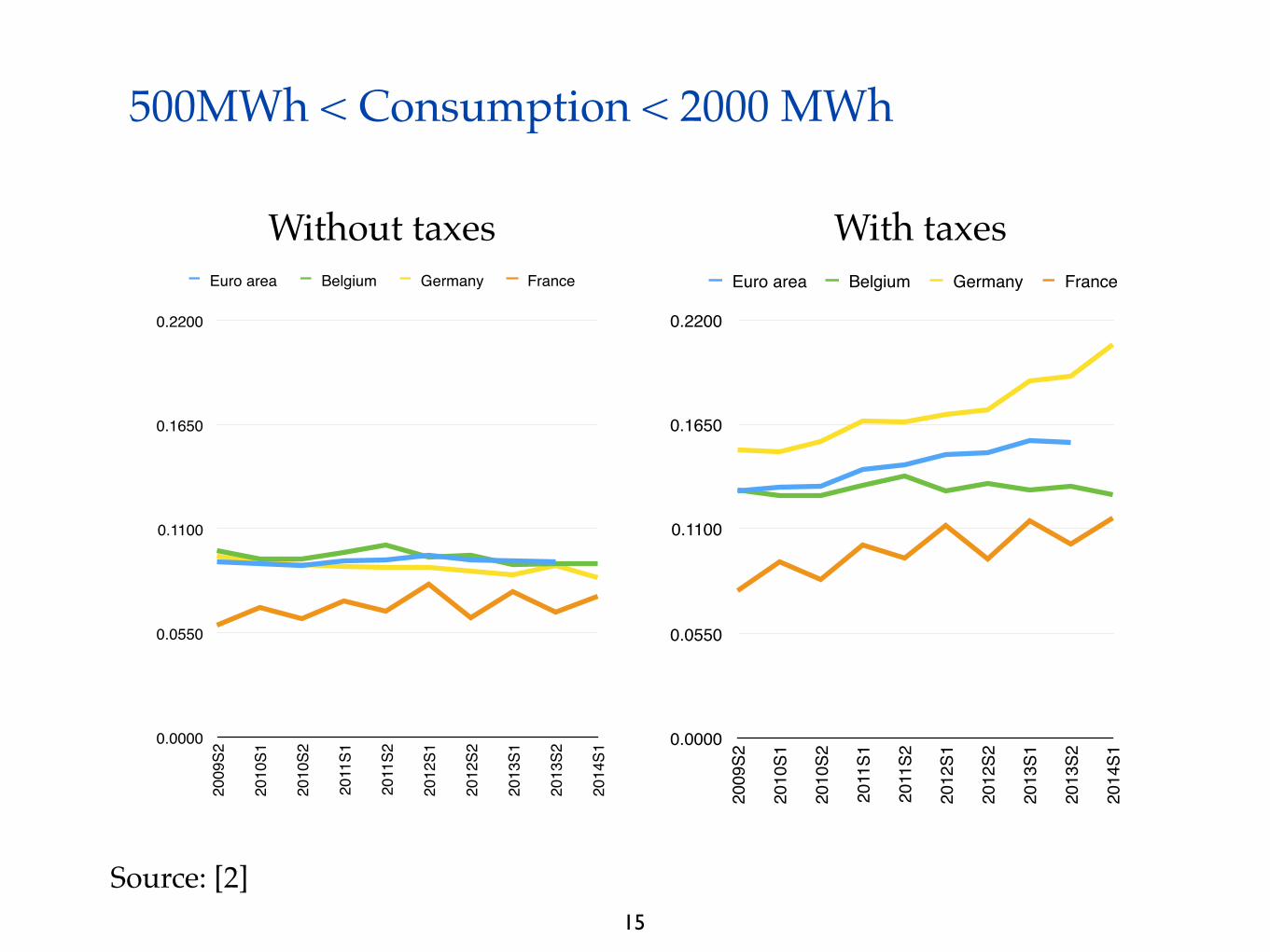
500MWh < Consumption < 2000 MWh
15
0.0000
0.0550
0.1100
0.1650
0.2200
2009
S2
2010
S1
2010
S2
2011
S1
2011
S2
2012
S1
2012
S2
2013
S1
2013
S2
2014
S1
Euro area Belgium Germany France
Without taxes
0.0000
0.0550
0.1100
0.1650
0.2200
2009
S2
2010
S1
2010
S2
2011
S1
2011
S2
2012
S1
2012
S2
2013
S1
2013
S2
2014
S1
Euro area Belgium Germany France
With taxes
Source: [2]

Electricity prices for household consumers [Euro/kWh]
16
0.0000
0.0750
0.1500
0.2250
0.3000
2009
S2
2010
S1
2010
S2
2011
S1
2011
S2
2012
S1
2012
S2
2013
S1
2013
S2
2014
S1
Euro area Belgium Germany France
0.0000
0.0750
0.1500
0.2250
0.3000
2009
S2
2010
S1
2010
S2
2011
S1
2011
S2
2012
S1
2012
S2
2013
S1
2013
S2
2014
S1
Euro area Belgium Germany France
Without taxes With taxes
Source: [2]

Outline of the lecture
1. Definitions and market rules
2. Selected topics in Mathematical Programming
3. Formalization of the day-ahead market coupling problem
4. A few words about the solution method implemented in EUPHEMIA
17

Outline of the lecture
1. Definitions and market rules
2. Selected topics in Mathematical Programming
3. Formalization of the day-ahead market coupling problem
4. A few words about the solution method implemented in EUPHEMIA
18

Orders: expressing the willingness to buy or sell
For now, assume• participants submit orders that can be
matched to any proportion• p0: price at which the order starts to be
accepted • p1: price at which the order is totally
accepted• only one period• the quantity is an energy amount,
expressed in MWh (MegaWatt X hour)
Price
Quantityq
p0
p1
accepted quantity
19
Later on, we will denote the fraction of q accepted by
4 Illustrative examplesCase 1:
• No reserve provision
• No peak price
• No storage
• Only a priori case (no settlement)
• No microgrid operator
Islanded operation ∆ curtailment
5 Getting in or out of the communityThe problem of coalitions ... can subgroups can generate more profit than the whole?
6 Investment in new devices
7 ConclusionCHP not considered but changes conclusion only if their is a heat distribution network, else itjust imposes extra constraint locally to entities.
x œ [0, 1]
ReferencesYannick Phulpin, Miroslav Begovic, Marc Petit, and Damien Ernst. A fair method for centralized
optimization of multi-TSO power systems. International Journal of Electrical Power and
Energy Systems, 31(9):482–488, 2009. ISSN 01420615. doi: 10.1016/j.ijepes.2009.03.014. URLhttp://dx.doi.org/10.1016/j.ijepes.2009.03.014.
Di Zhang, Nouri J. Samsatli, Adam D. Hawkes, Dan J L Brett, Nilay Shah, and Lazaros G.Papageorgiou. Fair electricity transfer price and unit capacity selection for microgrids. En-
ergy Economics, 36:581–593, 2013. ISSN 01409883. doi: 10.1016/j.eneco.2012.11.005. URLhttp://dx.doi.org/10.1016/j.eneco.2012.11.005.
16

A single period, single location, day-ahead market
Market Clearing Price (MCP)
Sell
Buy
Aggregated sell and buy curves
Price
Quantity
20

• But what are the properties of the computed prices? Ideally, they should be such that all orders that are
• in-the-money are fully accepted
• out-of-the-money are fully rejected
• at-the-money are accepted
• at a proportion if
• at any proportion if p0 = p1
“Clearing” the market amounts to determining which orders should be accepted and at which price
21
MCP � p0p1 � p0
p0 6= p1

Exercise with hourly order curves
• The order book is composed of
• Determine the supply and demand curves and compute the MCP.
22
Order Type Quantity p0 p1
1 Supply 10 0 20
2 Supply 15 10 25
3 Demand 5 30 10
4 Demand 10 30 30

Solution
23
0
7.5
15
22.5
30
0 7.5 15 22.5 30
Supply Demand
Market Clearing Price (MCP)
12.5 MWh

Graphical view of welfare (shaded area)
Sell
Buy
Surplus of buyersPrice
Quantity
24
Market Clearing Price (MCP)
Surplus of sellers

Block orders
A block order is defined by
• one price
• a set of periods
• quantities for those periods
• (a minimum acceptance ratio)
Why?
• Producers want to recover start-up costs, model technical constraints,
• consumers want to secure their base load.
Severe complications
• Couples periods
• Introduces “non-convexities”
25

Exercise with block orders (a single time period)
26
Price
Quantity
Optimizing welfare would lead to the acceptance of the two block orders.How do you set the price? Which orders are accepted?
Buy order 1
Buy order 2
Sell block order 2
Sell block order 1

The rule in Europe: no Paradoxically Accepted Block (PAB)
No order can be accepted while loosing money, even if it increases the total welfare.
On the other hand a block order could be rejected although it is in the money: Paradoxically Rejected orders.
Exercise: create an example where the optimal solution contains a Paradoxically Rejected Block order.
27

28
The exchanges between markets are restricted
Capacitated network flow
Belgium
France
The Netherlands
Germany
-Cdown ≤ flow(FR,DE) ≤ Cup
This is not a realistic model, since there are other transmission lines and power flows according to Kirchhoff laws (non-linear).
ATC model: connectors are defined between some pairs of bidding areas.Electricity can be exchanged via these connectors, but exchanges are limited.

Two markets, no congestion
29
Price
Quantity
Price
Quantity
Market A Market BInfinite capacity

Two markets, no congestion
29
Price
Quantity
Price
Quantity
Uniform global price
Market A Market BInfinite capacity

Two markets, no congestion
29
Price
Quantity
Price
Quantity
Market B exports to market A (all demand matched from supply of market B)
Uniform global price
Market A Market BInfinite capacity

Two markets, no congestion
29
Price
Quantity
Price
Quantity
Price
Quantity
As if there were only one market
Market B exports to market A (all demand matched from supply of market B)
Uniform global price
Market A Market BInfinite capacity

Two markets, congestion
30
Price
Quantity
Market A
Price
Quantity
Market B
Transfer limited
Price difference
Max 10 MW

Two markets, congestion
30
Price
Quantity
Market A
Price
Quantity
Market B
Transfer limited
Market B exports to market A, but not enough to equalize prices
Price difference
Max 10 MW

Refining the network model
Flow based model
• Instead of an ATC model, a more realistic representation is achieved by expressing linear constraints on net exports of bidding areas
• Coefficients of net exports, called Power Distribution Coefficient Factors (PTDF), are obtained thanks to an approximate sensitivity analysis around the expected working point of the system
• Issues with the economic interpretation of prices
Losses and tariffs on DC inter-connectors
Network ramping, ...
31

“Flow based” network model
Goals:
• express better the physical constraints of the network
• Allocate more capacity
• increase welfare
32

How?
A set of critical branches (CBs) are considered. Critical branches are lines, cables or devices that can be heavily impacted by cross-border exchanges. These are not only cross-border lines.
The expected loading of CBs is evaluated based on long term nominations. Part of the remaining margin can be allocated to day-ahead markets.
The impact of cross border exchanges on CBs is modelled through the net export of the bidding areas in the same balancing area.
Balancing area: set of bidding areas for which sum of net exports is zero. Can exchange energy with other balancing area, but accounted in another variable. E.g. CWE, FR + BE + NL + DE
33

NordPool Spot
Linked blocks
• Acceptance of one block conditioned by acceptance of other blocks
Flexible blocks
• e.g. a block of one hour that may be accepted at any period
34

GME (Italy)
Italy is split in several sub-markets
We must determine one common clearing price for all demand orders whatever the sub-market m: PUN (Prezzo Unico Nazionale)
Supply orders are remunerated at zonal price Pm
Assume Qm is the quantity matched in zone m
Goal: zero imbalance
35

OMIE (Spain – Portugal – Morocco)
“Complex Order” defined by
• Several supply curves for several periods
• A Minimum Income Condition
• Bounded variations between consecutive periods
quantity matched
market price
Minimum Income
period
36

Price/volume indeterminacies
• When curves cross on a vertical segment, there is a price indeterminacy
• Rule: try to be as close as possible from the mid point of the intersection interval
• Similarly, when curves cross on a horizontal segment, there is a volume indeterminacy
• Rule: maximize traded energy
• Note: there are other curtailment rules (local matching, ...)
37

Outline of the lecture
1. Definitions and market rules
2. Selected topics in Mathematical Programming
3. Formalization of the day-ahead market coupling problem
4. A few words about the solution method implemented in EUPHEMIA
38

Optimization
39
Find the best solution to a problem (the best according to a pre-specified measure, a function) and satisfying some constraints.
Example: find the longest meaningful word composed of letters in the set{T,N,E,T,E,N,N,B,A}
https://www.youtube.com/watch?v=lsFAokXCxTI
The problem is usually cast in mathematical language.
The solution method is usually automatic, that is an algorithm implemented on a computer.

Linear programing (LP)
Objective and constraints are linear expressions, and variables have continuous domains.
Example:
Properties:
•The feasible domain is a polyhedron.
•Optimal solution(s) lie on the boundary of that polyhedron.
40

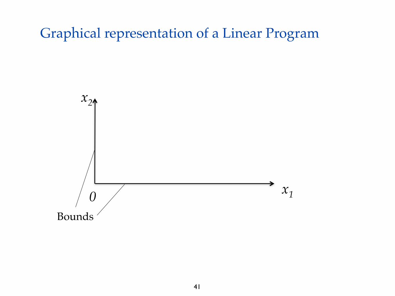
Graphical representation of a Linear Program
41
x2
x1 0
Graphical representation of a Linear Program
41
x2
x1 0Bounds

Graphical representation of a Linear Program
41
x2
x1 0
Constraints
6Bounds
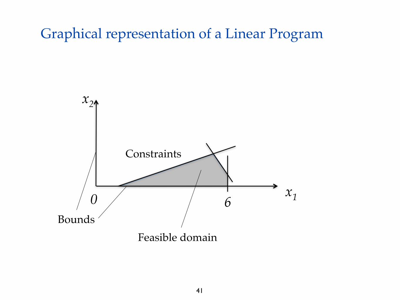
Feasible domain
Graphical representation of a Linear Program
41
x2
x1 0
Constraints
6Bounds

Feasible domain
Graphical representation of a Linear Program
41
Objective increases in this direction x2
x1 0
Constraints
6Bounds
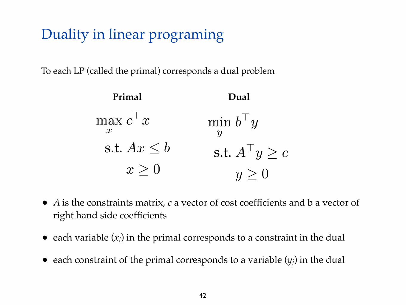
To each LP (called the primal) corresponds a dual problem
Duality in linear programing
42
max
x
c
>x
s.t. Ax b
x � 0
Primal
miny
b>y
s.t. A>y � c
y � 0
Dual
• A is the constraints matrix, c a vector of cost coefficients and b a vector of right hand side coefficients
• each variable (xi) in the primal corresponds to a constraint in the dual
• each constraint of the primal corresponds to a variable (yj) in the dual

Complementary slackness
At optimality, the following relations hold:
For all rows i and all columns j of A, where ai is row i of matrix A and Aj is column j of matrix A (vectors are always understood as column vectors)
This means that, at optimality, either a primal (resp. dual) constraint is tight (satisfied to equality) or the corresponding dual (resp. primal) variable is zero.
43

Solving very large LPs
Simplex
• moves from one vertex (extreme point) of the feasible domain to another until objective stops decreasing
• very efficient in practice but can be exponential on some special problems
• can keep information of one solution to quickly compute a solution to a perturbed problem (useful in a B&B setting), dual simplex, ...
Barrier
• iteratively penalizes the objective with a function of constraints, to force successive points to lie within the feasible domain
• polynomial time, very efficient especially for large sparse systems
• but no extremal solution hence crossover required in a B&B setting
44

Convex optimization
Those results generalize to problems more general than LP, that is when the objective and the feasible domain are convex.
There is a theoretical guarantee that there exist algorithms to solve those problems efficiently.
Example: (convex) Quadratic Programming (QP) are problems where the objective is quadratic and constraints are linear. The simplex and barrier algorithms can be adapted to QP.
45

Mixed Integer programing (MIP)
Idem as before, except that some variables must take integer values.
In general, relaxing the integrality requirement and solving the resulting continuous optimization problem does not yield a feasible solution to the original problem. Simple rounding procedures do not necessarily restore feasibility, and even if it does, do not guarantee optimality. However, the continuous relaxation provides a bound on the optimum of the original problem.
Simple enumeration of combinations of integer variable values is computationally undoable. Branch-and-bound is a clever way to do enumeration. It progressively imposes integer values and uses the solution to intermediate continuous relaxations to obtain bounds and thus avoid exploring some combinations, without losing optimal solutions.
46
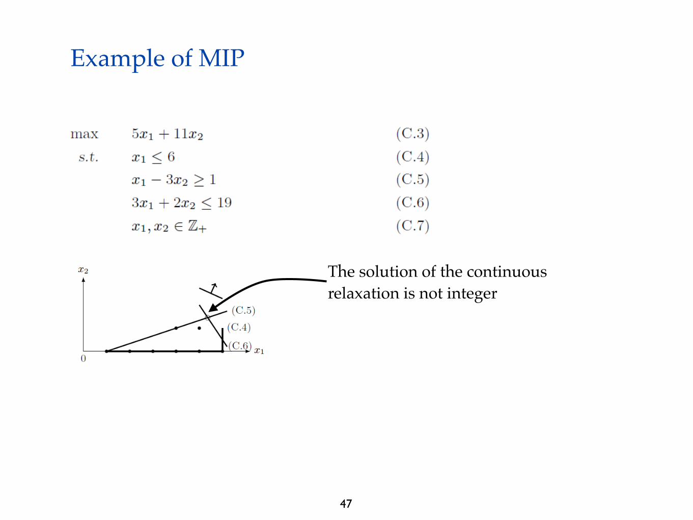
Example of MIP
47
The solution of the continuous relaxation is not integer

Branch and bound exampleFractional solution
48

Branch and bound exampleFractional solution
48

Branch and bound example
Fractional solution
Fractional solution
48

Branch and bound example
Fractional solution
Fractional solution
48

Branch and bound example
Fractional solution
Fractional solution
Integer solution48

Branch and bound example
Fractional solution
Fractional solution
Integer solution48

Branch and bound example
Fractional solution
Fractional solution
Integer solution
Prune by infeasibility
48

Branch and bound example
Fractional solution
Fractional solution
Integer solution
Prune by infeasibility
48

Branch and bound example
Fractional solution
Fractional solution
Integer solution
Prune by infeasibility
Prune by bound48

Outline of the lecture
1. Definitions and market rules
2. Selected topics in Mathematical Programming
3. Formalization of the day-ahead market coupling problem
4. A few words about the solution method implemented in EUPHEMIA
49

Features considered in the remainder of this lecture
• ATC coupling problem with hourly orders and block orders only.
• I.e. we do not consider GME, OMIE, smart orders, nor flow based network model.
50
Nature of the mathematical problem
It is a mathematical program with complementarity constraints (MPCC) and in addition it contains integer decision variables.
It enters the category of Mixed Integer Non-Linear Programs, meaning that the continuous relaxation of the problem is non-convex.
As we will see in the next section, Euphemia approximates the problem as a Mixed Integer Quadratic Program (MIQP) that is convex (Q is positive semi-definite) and then checks the solution is compliant with the “true” problem.
51

The primal market coupling problem
Clearing constraints express the equality of generation and demand
Main decision variables:
• acceptance ratio of orders
52
maximize Welfare
subject to 1. Clearing Constraints
2. Network constraints
3. Order definition constraints

Objective function: maximize social welfare
Exercise (solution on next page): Assume each order i of a set I is defined by
• its quantity qi
• its start and end prices pi0 and pi1
• its type (supply or demand)
Write down the expression of welfare as a function of accepted quantities (for simplicity, do not account for block orders).
53
54
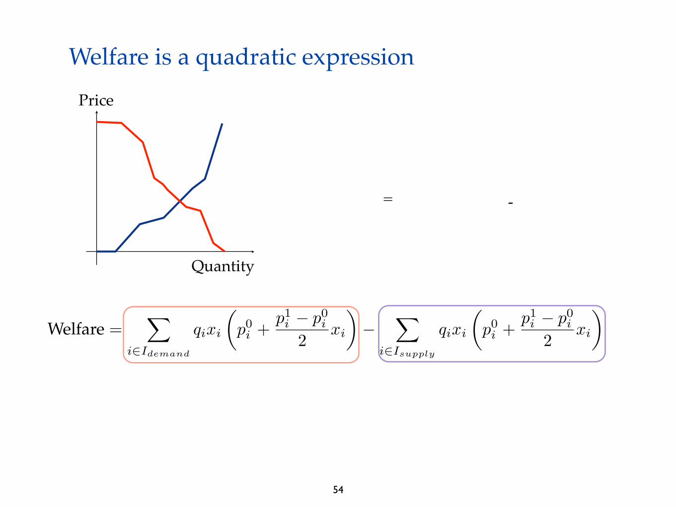
Welfare is a quadratic expressionPrice
Quantity
= -

54
Welfare is a quadratic expressionPrice
Quantity
= -

54
Welfare is a quadratic expressionPrice
Quantity
= -

54
Welfare is a quadratic expressionPrice
Quantity
= -

54
Welfare is a quadratic expressionPrice
Quantity
= -

Exercise
Define the necessary variables and formulate all the primal constraints (clearing, ATC, block order definition).
55

56
Without block orders, the problem has the following properties
• The formulation is convex (QP) and can be decomposed hour by hour
• Dual solution yields market prices and congestion prices
Primal constraints Dual variables
Clearing Market Clearing Price (MCP)
Inter-connector capacity Inter-connector congestion price
Orders acceptance UB Order “surplus” (Si)
57
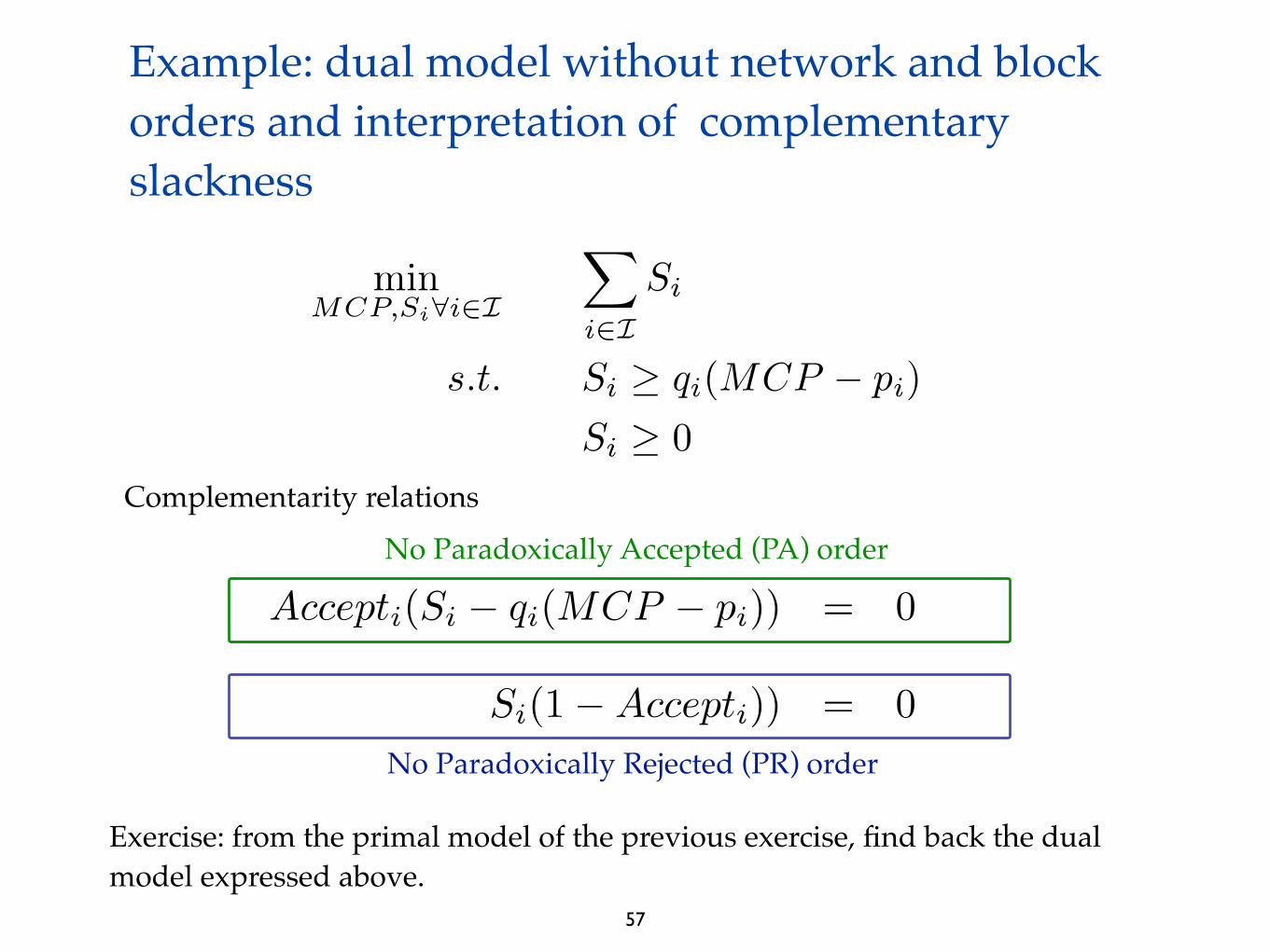
Example: dual model without network and block orders and interpretation of complementary slackness
No Paradoxically Accepted (PA) order
No Paradoxically Rejected (PR) order
Complementarity relations
Exercise: from the primal model of the previous exercise, find back the dual model expressed above.

58
Solutions naturally satisfy market rules
Order type MCP Acceptance Ratio
supply > p1 1
supply < p0 0
any >= p0 and <= p1 (MCP-p0) / (p1-p0)
demand < p1 1
demand > p0 0

59
Incorporating block orders
Complications
integer variables, thus QP à MIQP
time coupling
Paradoxically Accepted Blocks (PAB)
Market says it is not acceptable to lose money, but it is acceptable to be rejected although could have made money, without compensation

Outline of the lecture
1. Definitions and market rules
2. Selected topics in Mathematical Programming
3. Formalization of the day-ahead market coupling problem
4. A few words about the solution method implemented in EUPHEMIA
60

About Euphemia
• Property of PCR members
• Developed by n-Side
• In operation since February 4, 2014. Before that the former solution COSMOS operated from November 9 2010 in the CWE region.
• Now almost 4 years without failure• Typical size of instances:• 50.000 orders• 700 blocks• COSMOS solved real instances in less than 10 seconds. Now
the algorithm takes several minutes.
61

Main idea
For a fixed selection of blocks, the Market Coupling Problem can be written as a QP
Solving this problem yields
• quantities (primal)
• prices (dual)
If there is no PAB with respect to those prices
• the block selection and the prices form a feasible solution to the Market coupling problem
Else we must find another block selection.
62

Branch-and-cut algorithm description (1)
Integer
Primal
When a node yields an integer solution for the primal
63

Branch-and-cut algorithm description (2)
Dual constraints
Set bounds on dual variables by
complementarity
Dual
The dual of the relaxed problem (integer variables fixed) is constructed from the primal solution by complementarity
Integer
Primal
64

Branch-and-cut algorithm description (3)
Dual constraints
Dual
Integer
Primal
+ no PAB constraints
A constraint preventing prices that cause PAB is appended to the dual problem
65

Branch-and-cut algorithm description (4)
Dual constraints
Dual
Integer
Primal
+ no PAB constraints
The objective is modified to yield prices as close as possible to the center of the price indeterminacy intervals
Price problemModified objectiveto lift price indeterminacies
66

Branch-and-cut algorithm description (5)
Dual constraints
Set bounds on dual variables by
complementarity
Dual
Integer
Primal
+ no PAB constraints
if that problem is feasible, we have a candidate solution for the market coupling problem
Price problemModified objectiveto lift price indeterminacies
Feasible
Acceptable
67

Branch-and-cut algorithm description (6)
Dual constraints
DualPrimal
+ no PAB constraints
Else a cut is added to the current node to prevent this block selection
Price problemModified objectiveto lift price indeterminacies
Infeasible
68

About the implementation in Euphemia
• Implemented
• in Java
• using CPLEX and Concert Technology
• tuned cutting and node selection mechanisms
• achieves a precision of 10-5 on all constraints
• Embedded mechanisms to repair numerically difficult problems
69

References
[1] EPEX spot annual report 2013
[2] Eurostat: http://appsso.eurostat.ec.europa.eu/nui/setupDownloads.do
70