How to capture more ILP - Page d'accueil / Lirmm.fr / - lirmm · How to capture more ILP B. Goossens, LP2A/DALI Archi07, Boussens, 19-23 mars 2007

How to capture more ILP

B. Goossens, LP2A/DALI

Archi07, Boussens, 19-23 mars 2007

Instruction Level Parallelism

● Natural program parallelism.

● Enhancing parallelism for the data path.

● Enhancing parallelism for the instruction path.

● The ILP wall.

● How can we break the ILP wall?

ILP in the SAXPY procedure

forall (i=0; i<1024; i++) y[i] += x[i] * a;

The source code is parallel as long as it is written in an appropriate language (e.g. Unified Parallel C).

In this code, there are 1024 independent computations (fix i , load x[i] , multiply, load y[i] , add, store y[i] ).

An ad hoc hardware

Saxpy 1024 in 4 cycles (load x, multiply and load y, add, store) (1024 +, 1024 *).

xy

0 1023

l/e x/y a

*

+

l/e x/y a

*

+

SAXPY in machine code

// x in R8, y in R9, n (1024) in R10, i in R1, i-n in R2

// a in F1, x[i] in F2, y[i] in F3, a*x[i] in F4, y[i]+a*x[i] in F5

saxpy ADD R1, 0, 0

loop FLOAD F2, R8(R1)

FLOAD F3, R9(R1)

FMUL F4, F1, F2

FADD F5, F3, F4

FSTORE F5, R9(R1)

ADD R1, R1, 1

SUB R2, R1, R10

BNE R2, loop

The machine code is not parallel.

There is only one singlecomputation made of 1 + 8*1024inter-dependent instructions.

Why isn't the new code parallel?● Introduction of control (e.g. loop):

Instructions run after a conditional or indirect branch depend on the branch.

● Introduction of shared registers:

Instructions writing to and reading from register r depend on instructions writing to r .

● Introduction of the load-store model:

Instructions writing to and reading from memory address b depend on instructions writing to memory address a until a and b are known.

How can we regain the lost parallelism?

● Speculate (start a dependent computation, assuming the dependency condition is solved).

● Remap (expand the architectural set of resources and remap the code on the new set, removing part of the dependencies).

How can we regain the lost parallelism?

● Predict conditional branch direction and indirect jump target (branch predictor and target buffer).

● Expand the set of shared registers and remap the machine code onto the new set (register renaming).

● Speculate on load addresses (speculative loads).

SAXPY in-order computation

● Instruction i starts its computation when its dependencies with instructions j<i are solved and when instruction i-1 is started (pipelining accelerates the process).

1,0 1,1 1,2 1,3 1,4 1,5 1,6 1,7 1,8

2,1 2,2 2,3 2,4 2,5 2,6 2,7 2,8

i, j: instruction j in iteration ij<i: j precedes i

Distance from(i,j) to (i+1,j)is 8.

SAXPY in partial order computation

● Instruction i starts its computation when its dependencies with instructions j<i are solved (superscalar ooo execution).

1,01,1

1,2

1,3 1,4 1,5 1,6 1,7 1,8

2,1

2,2

2,3 2,4 2,5 2,6 2,7 2,8

control

WAR

RAW


Dependencies on registers

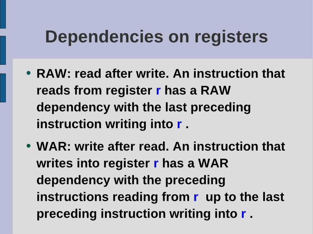
● RAW: read after write. An instruction that reads from register r has a RAW dependency with the last preceding instruction writing into r .

● WAR: write after read. An instruction that writes into register r has a WAR dependency with the preceding instructions reading from r up to the last preceding instruction writing into r .

Dependencies on registers

● WAW: write after write. An instruction that writes into register r has a WAW dependency with the last preceding instruction writing into r .

● WAW and WAR dependencies can be removed by remapping (duplicate reg.).

● RAW and WAR dependencies can be removed by speculating (predict rather than read).

SAXPY with branch prediction

● Instruction i starts its computation when its dependencies with instructions j<i are solved. Speculate on branch direction.

1,01,1

1,2

1,3 1,4 1,5 1,6 1,7 1,8

2,1

2,2

2,3 2,4 2,5 2,6 2,7 2,8


Need to correctfalse predictions.

Branch prediction in the SAXPY loop

● Speculate on the direction of the loop branch (bet it will be taken).

● Next iteration does not depend anymore on the branch computation.

● At the end of the 1024 iterations, the bet is lost. It is required to correct: the code following the loop has a dependency with the branch.

Impact of branch prediction on SAXPY ILP

● Control dependencies are removed.

● The next iteration starts when the loop counter is updated (instruction (i, 6)), which cannot be performed sooner than after the current iteration store because of the WAR dependency on the loop counter register.

● Small impact.

Hints to the programmer to enhance ILP with branches

● Reduce conditional branches in the static code (they are frequent in iterative programming). e.g. unroll loops, avoid very few iterations loops, use conditional moves.

● Reduce conditional branches in the dynamic code, e.g. sort successive branches from the most taken one to the least.


● Favour highly predictable branches (either one dominating direction -e.g. taken for a loop with many iterations- or one dominating path for a succession of branches -e.g. when one branch is taken, next one is also mostly taken -.

● Impact of conditional branches prediction correction on ILP is high: many branches (10% to 20%), mispredictions (2% to 8%).


● Reduce indirect branches in the static code (they are frequent in functional programming with return instructions). e.g. inlining.

● Return address predictors are very accurate and return instructions are not very frequent in the dynamic code (2%).

● Impact of indirect branches prediction correction on ILP is low.

SAXPY with renaming (no branch prediction)

● Instruction i starts its computation when its dependencies with instructions j<i are solved. Rename registers.

1,0 1,1

1,2

1,3 1,4 1,5

1,6 1,7 1,8

2,1

2,2

2,3 2,4 2,5

2,6 2,7 2,8

memory

Distance from(i,j) to (i+1,j)is 3 (control)or 4 (compute).

Register renaming

● Assume an infinite set of renaming registers.

● Any destination register is remapped to a unique renaming register.

● Any source register r is remapped to the renaming register assigned to r by the last preceding instruction having r as a destination.

Register renaming

● WAW dependencies are removed as instructions write in a unique renaming register.

● WAR dependencies are removed as instruction sources are read from a unique renaming register.

When may a renaming register be reused?

a: OP R1, R2, R3 //RR1 renames R1

...

b: OP R4, R1, R5 //RR1 used

...

c: OP R1, R6, R7 //RR2 renames R1

...

d: OP R8, R9, R0 //RR1 may rename R8 //if b has read RR1

Memory dependency

● A load potentially depends on any preceding store (RAW mem. dep.).

● The dependency is pending until the load and the store addresses have both been computed.

● The dependency is confirmed if both memory accesses concern at least one single common byte.

Memory dependency

● A store potentially depends on any preceding load (WAR mem. dep.) and on any preceding store (WAW mem. dep.).

● The dependency is pending until the addresses have both been computed.

● The dependency is confirmed if both memory accesses concern at least one single common byte.

Impact of register renaming on SAXPY ILP

● WAR + WAW dependencies are removed.

● It builds two parallel sequences: the control part (loop counter computation), sequentialized by a control dependency; the loop body part, sequentialized by a memory dependency (the next iterations loads cannot be performed before the current iteration store).

● Average impact

Hints to the programmer to enhance ILP with renaming

● The only limitation to ILP introduced by the renaming process is due to the finite number of renaming registers.

● Instructions with no destination (e.g. store and branch) allocate no register (not a hint, just a note).

● Remanent data keep registers allocated for a long time. Favour volatile data. (in SAXPY, a is remanent and i is volatile).

SAXPY with renaming and memory address speculation

● Instruction i starts when its dependencies with instructions j<i are solved. Rename registers, speculate on memory address.

1,0 1,1

1,2

1,3 1,4 1,5

1,6 1,7 1,8

2,1

2,2

2,3 2,4 2,5

2,6 2,7 2,8


Need to correctfalse speculation.

Load address speculation

● The load is performed even though there are still some unkown preceding store addresses.

● When a store address is resolved, it is compared to the addresses of all the following loads already run.

● If a match occurs, the run is restarted from the incorrect load. This adds a RAW mem. dependency.

Store address speculation

● The store is performed even though there are still some unkown preceding load or store addresses.

● When a load or store address is resolved, it is compared to the addresses of all the following stores already run.

● If a match occurs, the run is restarted from the incorrect load or store. This adds a WAR or WAW mem. dependency.

Impact of renaming and mem. speculation on SAXPY ILP

● WAR + WAW dependencies are removed.

● Memory load dependencies are removed.

● The loop body part for the next iteration is artificially relinked to the current iteration loop counter part by the control dependency.

● Low impact compared to renaming only.

Hints to the programmer to enhance ILP with mem. spec.

● Impact of memory speculation correction on ILP may be high: many stores (10% to 20%).

● Mispredictions occur when there is a true RAW dependence between a store and the following loads.

● Avoid to read a variable that has been just written (e.g. avoid a recurrence on a variable in memory; avoid push/pop).

SAXPY with b. prediction, renaming and m. speculation

1,0 1,1

1,2

1,3 1,4 1,5

1,6 1,7 1,8

2,1

2,2

2,3 2,4 2,5

2,6 2,7 2,8


What is the ILP limit in SAXPY with b. pred., r. ren., m. spec.

● Because instruction (i+1, 6) has a RAW dependency on R1 with instruction (i, 6), the distance between two successive iterations is at least 1.

● Hence, instruction (i+1, j) has at least a distance of 1 with instruction (i, j) (in SAXPY, all the instructions in the loop body depend on the iteration counter).

What is the ILP limit in SAXPY with b. pred., r. ren., m. spec.

● Instructions (i, j) and (i+k, j) (k>0) cannot have a distance of 0.

● The set of distance 0 instructions (the ones that can be run in parallel) at most contains one of each instruction in the loop body.

● The ILP limit is the number of instructions in the loop body.

● To enhance ILP, unroll the loop.

SAXPY with value, branch and memory speculation

● e.g. In ld/st instructions, R1 is predicted rather than read in register (RAW and WAR dependencies on R1 are removed).

1,0

1,1

1,2

1,3 1,4 1,5

1,6 1,7 1,8

2,1

2,2

2,3 2,4 2,5

2,6 2,7 2,8

WAW


What is the ILP limit in SAXPY with b. pred., v. pred., m. spec.

● Because instruction (i+1, 6) has a RAW dependency on R1 with instruction (i, 6), the distance between two successive iterations is at least 1 (as when renaming is applied).

● The ILP limit is the number of instructions in the loop body.

How to remove dependencies

● Renaming removes WAR and WAW dependencies.

● Branch prediction (direction and target) removes control dependencies.

● Memory address speculation removes load after store dependencies.

● Value prediction removes WAR and RAW dependencies.

Fetching instructions in parallel

● The fetch bandwidth bounds the ILP that can be captured.

● The instructions should be fetched in-order to allow the dependency analysis.

● Fetching should be respectful of the control dependencies.

● Pipelined, superscalar, speculative fetching are needed techniques to provide enough instructions to the core.

Scalar fetching for SAXPY

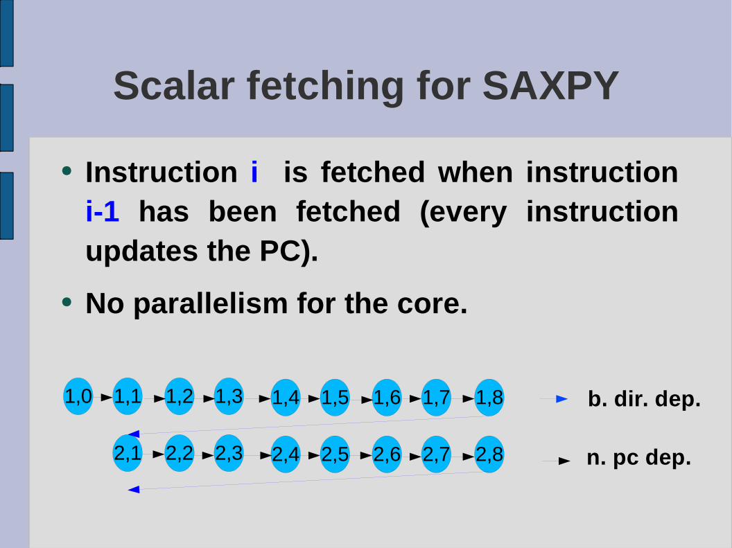
● Instruction i is fetched when instruction i-1 has been fetched (every instruction updates the PC).

● No parallelism for the core.

1,0 1,1 1,2 1,3 1,4 1,5 1,6 1,7 1,8

2,1 2,2 2,3 2,4 2,5 2,6 2,7 2,8

b. dir. dep.

n. pc dep.

Superscalar fetching for SAXPY(single basic block)

● Instructions in a Basic Block (bb) arefetched in parallel. Only the bb ending instruction updates PC. Next bb is fetched when the control dependency with the current bb has been solved.

1,0 1,1 1,2 1,3 1,4 1,5 1,6 1,7 1,8

2,1 2,2 2,3 2,4 2,5 2,6 2,7 2,8

Superscalar fetching

● The parallelism offered to the core is bounded by the average basic block size.

● In 5 SPECInt2000 benchmarks, there are 15% of branch/call/return instructions run (average bb size: 6 instructions).

● In 5 SPECfp2000 benchmarks, there are 4% of branch/call/return instructions run (average bb size: 25 instructions).

Superscalar fetching

● The parallelism offered to the core is also bounded by the instruction memory bus width (the superscalar fetching degree).

● A bb can span multiple memory accesses (large basic blocks) or can occupy a small part of a memory access (small bb).

● Bus expansion increases the parallelism offered to the core, up to the average bb length.

Superscalar fetching for SAXPY (4 instructions memory bus)1,0 1,1 1,2 1,3

1,4 1,5 1,6 1,7

1,8

2,1 2,2 2,3

2,4 2,5 2,6 2,7

2,8 x xx

x

x xx

x xx x xx

4 aligned instructions fetched


1 aligned instruction fetched



1 aligned instruction fetched

average (2/3 of bus) 2,66 aligned instructions fetched

pc ++ computation dependency




b. dir. computation dependency

Fetched lines dependencies

● PC++ computation.

● Branch direction computation or prediction.

● Indirect jump computation (e.g. pop the return address) or prediction (e.g. pop the return address from a small hardware stack).

Superscalar fetching for SAXPY (8 instructions memory bus)1,0 1,1 1,2 1,3 1,4 1,5 1,6 1,7

1,8

2,1 2,2 2,3 2,4 2,5 2,6 2,7

2,8 x xx

x

x xx

x xx x xx x xx x xx x

x xx x xx x

average (½ of bus) 4 aligned instructions fetched

8 instructions

1 instruction

7 instructions

1 instruction

Superscalar fetching for SAXPY (16 instructions memory bus)1,0 1,1 1,2 1,3 1,4 1,5 1,6 1,7

1,8

2,1 2,2 2,3 2,4 2,5 2,6 2,7

2,8 x xx

x

x xx


x xx x xx x

9 instructions

8 instructions

average (½ of bus) 8 aligned instructions fetched

Further expansion of the memory bus is useless

Compiler hints to improve superscalar fetching

● Decrease the number of branch instructions (conditional move, loop unrolling).

● Align the code (in SAXPY, align the loop body).

● Decrease the number of indirect jumps (inlining, transform recursion into iteration when possible).

SAXPY with aligned body loop (8i bus)

1,0

1,1 1,2 1,3 1,4 1,5 1,6 1,7 1,8

2,1 2,2 2,3 2,4 2,5 2,6 2,7 2,8


3,1 3,2 3,3 3,4 3,5 3,6 3,7 3,8

Superscalar fetching for SAXPY(multiple basic blocks)

● Multiple bb are fetched in parallel. Only the ending instruction of the last bb updates PC. Next set of bb is fetchedwhen the control dependency with the last currently fetched bb has been solved.

● The control dependencies between the fetched bb are solved by prediction. The predictor must provide the starting address of each of the bb to be fetched.

Multiple block ahead predictor

● For n fetched blocks, the predictor must deliver n bb addresses (PC gives the first bb address, the predictor gives next PC).

● The inner dependencies to solve can be any mix of conditional branch targets, function calls (return address to be pushed), return addresses, immediate or indirect jumps.

Multiple block ahead predictor

● A major simplification is to concentrate the prediction on the conditional branches.

● When a bb is ended by an indirect jump, this bb ends the set of fetched bb.

● Still, we can fetch multiple function calls (push all the return addresses) and a last bb ended by a return (pop the last address pushed in the same fetch cycle).

Two bb fetch in SAXPY (two branch predictions, 16i bus)

1,0 1,1 1,2 1,3 1,4 1,5 1,6 1,7

1,8 2,1 2,2 2,3 2,4 2,5 2,6 2,7

2,8 3,1 3,2 3,3 3,4 3,5 3,6 3,7

3,8 4,1 4,2 4,3 4,4 4,5 4,6 4,7

Compiler alignmentis no more required.

How many branch predictions are needed?

● The distribution of control flow instructions is not uniform.

● Integer codes have much more control flow instructions than floating point codes.

● With n predictions, on Int codes, we fetch 6n instructions on the average. On fp codes, we fetch 25n instructions on the average.

Available ILP in programs

● Maximum available ILP can be measured on a perfect processor (remove all dependencies except true data (register RAW); no value prediction).

● Perfect processor: Infinite renaming registers, perfect branch prediction, perfect load/store speculation, infinite issue and run capacity, single cycle execution.

ILP in SPEC92 (source: Hen-Pat Comp. Arch. 3rd edition, 2003)

The ILP wall

● A lot of ILP, but difficult to catch (low ILP programs should be parallelized).

● Resources must be provided to remove dependencies and to run in parallel with a short latency.

The window size limit

● The window is the set of consecutive instructions starting from the oldest uncompleted one.

● The perfect processor assumes an infinite window but a real processor has a fixed size window.

● Any instruction out of the window has a window limit dependency. The ILP suffers from such dependencies.

ILP in a fixed size window processor (source Hen-Pat'03)

The branch prediction limit

● The perfect processor assumes a perfect branch prediction but a real processor has an imperfect branch predictor.

● The state-of-the-art predictor (97% hits) is hybrid, predicting both the loop branches (local predictor) and the context-path branches (global predictor).

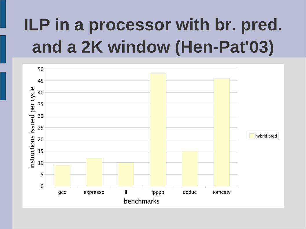
ILP in a processor with br. pred. and a 2K window (Hen-Pat'03)

ILP in a bounded processor

● 128 instructions window. Up to 64 issues per cycle. Single cycle latency operations. State-of-the-art branch predictor. Perfect memory address speculation.

● Can the ILP wall be crossed? Actual IPC is 2 in a 6-wide issue processor. There is still a lot of uncaught ILP (from 2 to 10).

ILP in a bounded proc. (128 inst. window) (Hen-Pat'03)

How can we break the ILP wall?

● Fetch must provide more on-the-path instructions to the data path.

● Decrease the misprediction rate (improve prediction techniques).

● Decrease the misprediction penalty (accelerate branch computation).

● Increase the fetch bandwidth (multiple bb fetch and multiple branch predictions).

How can we break the ILP wall?

● The data path must be improved to be more fully active and must be widened.

● To catch the available ILP (say n), every cycle a set of at least n independent instructions must be issued.

● These n instructions get their sources from the data path or from the registers.

● These n instructions put their results into the data path and in the registers.

Volatile and remanent data

● A datum is volatile from the time it is sent out of its computing unit until it is written to its destination register or discarded.

● A datum is remanent from the time it is written to its destination register until the same register is overwritten.

● The source of an instruction is volatile if the datum it depends on (RAW) is volatile. It is remanent if the datum is remanent.

Data writing into registers

● A datum is written into its destination register only if no later instruction is writing into the same register.

● When a set of instructions are committed together, if two write to the same register, only the latest one is performed.

● On 10 Mibench benchmarks, less than 1 write per cycle is performed. It decreases when the commit width increases.

Remanent writes (source Parello et al. Sympa'06)

Result writing and remanent data

● When a datum is written into its destination register, it becomes remanent.

● Later dependent sources will have to be read from the register file.

● Until it is either written or discarded, a result is a volatile datum.

● A volatile datum is forwarded to all the dependent sources (RAW).

Volatile and remanent data in SAXPY

saxpy ADD R1, 0, 0

loop FLOAD F2, R8(R1) R1 volatile, R8 remanent

FLOAD F3, R9(R1) R1 volatile, R9 remanent

FMUL F4, F1, F2 F1 remanent, F2 volatile

FADD F5, F3, F4 F3 and F4 volatile

FSTORE F5, R9(R1) R1 and F5 volatile, R9 remanent

ADD R1, R1, 1 R1 volatile

SUB R2, R1, R10 R1 volatile, R10 remanent

BNE R2, loop R2 volatile

Volatile and remanent data

● On 10 Mibench benchmarks, less than 30% of the sources are remanent.

● When the issue width is increased, the proportion of remanent data decreases.

● This is because the latency between production and consumption is reduced, turning remanent data into volatile ones.

Remanent sources (Parello et al, Sympa'06)

Volatile sources (Parello et al, Sympa'06)

A register file for a wide issue processor

● Should be placed out of the data path.

● Read remanent sources at dispatch, write remanent results at commit. No reg access from issue to writeback.

● 4-issue processor => 2 r and 1 w ports.



● Scalable register file.

Critical volatile sources

● A volatile source is critical if it is the ultimate source of the instruction (when the source is received, the instruction is ready to be issued).

● Critical sources are produced ooo.

● In 10 Mibench benchmarks, a 4-issue processor receives 3.8 critical volatile sources and 0.7 non critical volatile sources per cycle.

Critical volatile sources

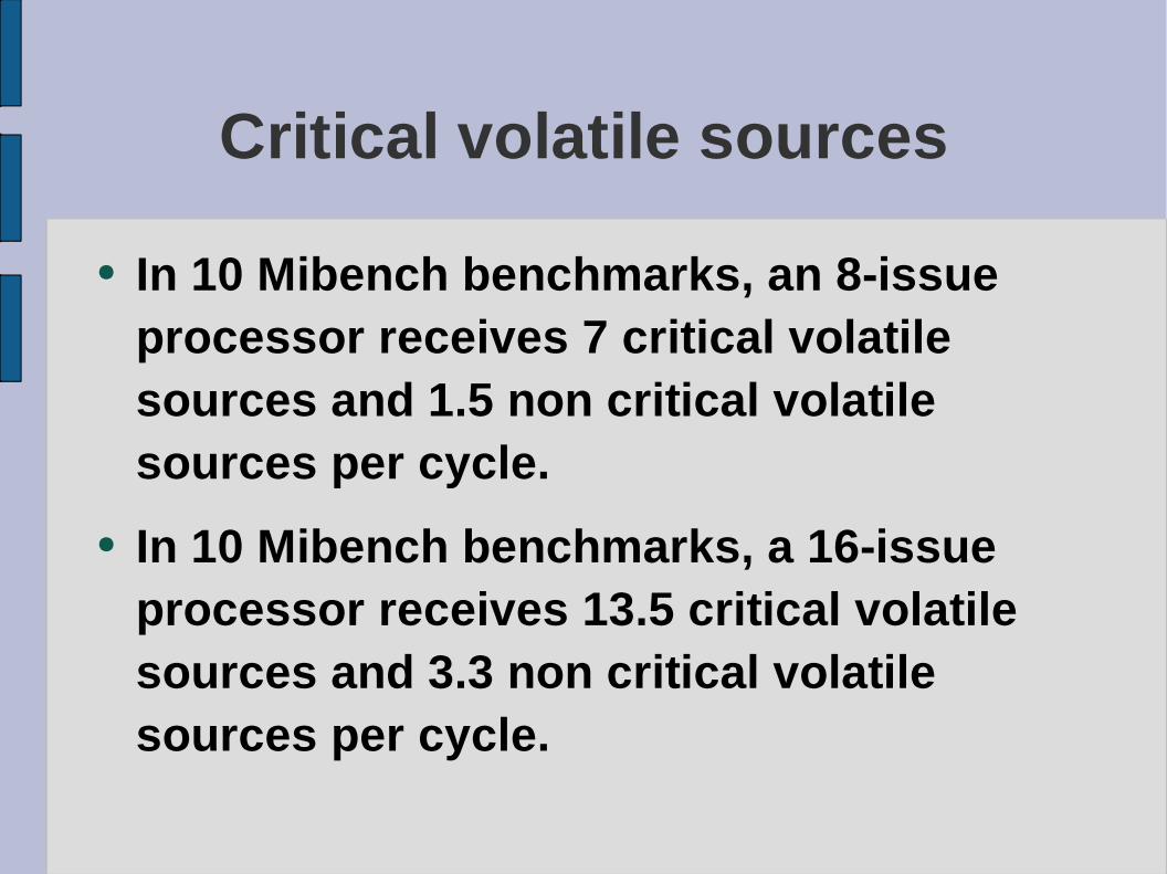
● In 10 Mibench benchmarks, an 8-issue processor receives 7 critical volatile sources and 1.5 non critical volatile sources per cycle.

● In 10 Mibench benchmarks, a 16-issue processor receives 13.5 critical volatile sources and 3.3 non critical volatile sources per cycle.

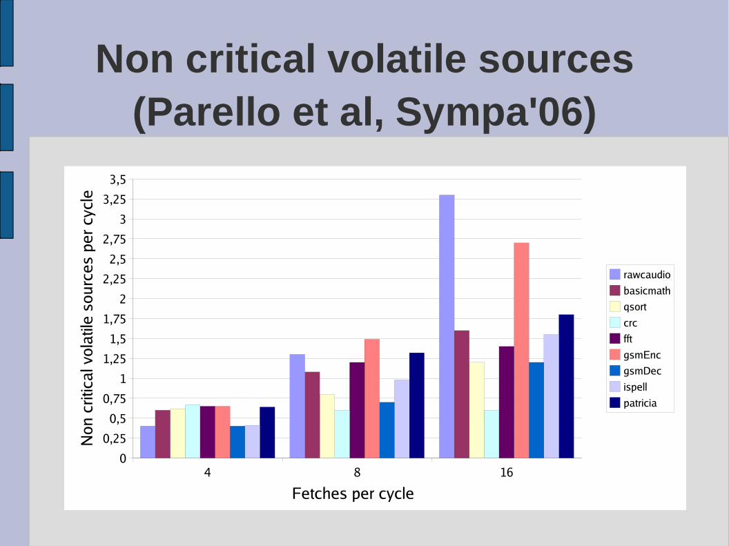
Non critical volatile sources (Parello et al, Sympa'06)

Critical volatile sources (Parello et al, Sympa'06)

A bypass network for a wide issue processor

● A bypass network routes the critical volatile data from the computing units output to the computing units inputs.

● An instruction is issued when its last source is scheduled for output.

● Each computing unit is linked to a small subset to allow the most frequent bypasses.

● The dispatcher maps dependent instructions on linked units (if any is suitable).

A forwarding network for a wide issue processor

● Non critical volatile data are routed from the computing units outputs to the waiting sources (issue stage).

● As the data are not critical, the route can be pipelined.

● The scheduler states which data are critical. It posts a routing protocol for every volatile source at the producer unit output.

Conclusion

● Programs have high ILP (or can be re-written to enhance their ILP).

● There are some hints to think that the processor issue width is scalable.

● We need more knowledge on how to schedule the instructions to optimize the captured ILP.

● We need to decrease the impact of branches (feed the data path with instructions).

Documents

How to capture more ILP - Page d'accueil / Lirmm.fr / - lirmm · How to capture more ILP B. Goossens, LP2A/DALI Archi07, Boussens, 19-23 mars 2007