How to Compute Equilibrium Prices in 1891 - Yale Universitydido.econ.yale.edu/~hes/pub/how-to-compute.pdf · How to Compute Equilibrium Prices in 1891 By WILLIAM C. BRAINARD and HERBERT

How to Compute Equilibrium Prices in 1891

By WILLIAM C. BRAINARD and HERBERT E. SCARF*

ABSTRACT. Irving Fisher’s Ph.D. thesis, submitted to Yale Universityin 1891, contains a fully articulated general equilibrium model pre-sented with the broad scope and formal mathematical clarity associ-ated with Walras and his successors. In addition, Fisher presents aremarkable hydraulic apparatus for calculating equilibrium prices andthe resulting distribution of society’s endowments among the agentsin the economy. In this paper we provide an analytical descriptionof Fisher’s apparatus, and report the results of simulating the mechan-ical/hydraulic “machine,” illustrating the ability of the apparatus to“compute” equilibrium prices and also to find multiple equilibria.

I

Introduction

IRVING FISHER’S Ph.D. thesis, submitted to Yale University in 1891, isremarkable in at least two distinct ways. The thesis contains a fullyarticulated general equilibrium model presented with the broad scopeand formal mathematical clarity that we associate with Walras and hissuccessors. But what is even more astonishing is the presentation, inthe thesis, of Fisher’s hydraulic apparatus for calculating equilibriumprices and the resulting distribution of society’s endowments amongthe agents in the economy.

The American Journal of Economics and Sociology, Vol. 64, No. 1 ( January, 2005).© 2005 American Journal of Economics and Sociology, Inc.

*William Brainard is the Arthur M. Okun Professor of Economics at Yale University.

A graduate of Oberlin College and Yale University, his research is primarily in macro-

economics. He is a Fellow of the Econometric Society and co-editor of the Brookings

Papers on Economic Activity. Herbert E. Scarf is the Sterling Professor of Economics at

Yale University. He received his Ph.D. in Mathematics from Princeton in 1954. He was

at the RAND Corporation from 1954 to 1956, and taught in the Department of Statis-

tics at Stanford from 1956 to 1963. In 1963, Scarf joined the Department of Econom-

ics at Yale and the Cowles Foundation. He received the Lanchester Prize of the

Operations Research Society of American in 1974 and the von Neumann Medal in 1983.

He is a member of the National Academy of Sciences and the American Philosophical

Society and is a Distinguished Fellow of the American Economic Society.

Fisher’s development of the general equilibrium model was donewithout any knowledge of the simultaneous achievement of Walras.In the introduction to his thesis, Fisher states that

[t]he equations in Chapter IV, Sec. 10, were found by me two years ago,when I had read no mathematical economist except Jevons. They werean appropriate extension of Jevons’ determination of the exchange of twocommodities between two trading bodies to the exchange of any numberof commodities between any number of traders. . . . These equations areessentially those of Walras.

Even though Fisher’s construction of what we now call the Walrasian model of equilibrium was a fully original achievement, hedid have contemporaries: the central ideas of equilibrium theory wereindependently discovered at several locations in the final decade ofthe last century. But the second theme of Fisher’s thesis was entirelynovel in conception and execution. No other economist of his timesuggested the possibility of exploring the implications of equilibriumanalysis by constructing specific numerical models, with a moderatelylarge number of commodities and consumers, and finding those pricesthat would simultaneously equate supply and demand in all markets.The profession would have to wait until rudimentary computers wereavailable in the 1930s before Leontief turned his hand to a simplifiedversion of this computation.

Fisher’s hydraulic machine is complex and ingenious. It correctlysolves for equilibrium prices in a model of exchange in which eachconsumer has additive, monotonic, and concave utility functions, anda specified money income; the market supplies of each good areexogenously given. Both additivity and fixed money incomes makethe model of exchange to which his mechanism is applied less thancompletely general. But we know of no argument for the existenceof equilibrium prices in this restricted model that does not requirethe full use of Brouwer’s fixed point theorem. Of course fixed pointtheorems were not available to Fisher and in that section of his thesisin which first-order conditions are presented for a general model ofexchange, Fisher argues for consistency by counting equations andunknowns.

It is hard to discover the source of Fisher’s interest in computation.He was a student of J. Willard Gibbs, and perhaps the theme of

58 The American Journal of Economics and Sociology

concrete models in mechanics was carried over to economics. But itis also possible that his hydraulic apparatus is simply an instance ofan American passion for complex machinery that gets things done.Fisher, himself, had a passion for innovation. In the course of a longcareer, he invented an elaborate tent for the treatment of tuberculo-sis (described in the Journal of the American Medical Association,1903), developed a mechanical diet indicator that permited easy cal-culation of the daily consumption of fats, carbohydrates, and proteins,copywrited (1943) an icosahedral world globe with triangular facetsthat when unfolded was allegedly an improvement on the Mercatorprojection, and patented an “index visible filing system” (1913) soldto Kardex Rand, later Remmington Rand, in 1925 for $660,000.

II

Fisher’s Cisterns

LET US BEGIN by describing the special model of exchange that is solvedby the Fisher machine. There are, say, m consumers, indexed by i = 1, . . . , m and n goods, indexed by j = 1, . . . n. Consumer i hasthe utility function

with each uij increasing and concave. Society’s endowment of goodj is Ej, and consumer i ’s income is Yi.

At prices p = (p1, . . . , pn) ≥ 0, consumer i is assumed to maximizeutility subject to his budget constraint

If the marginal utility of income for consumer i is li, the demands,xij, will satisfy the first order conditions:

A competitive equilibrium is given by a price vector p so that themarket demands obtained by the summation of individual demands

¢ ( ) £ = >( )u x p xij ij i j ijl if 0 .

max , . . . ,

.,

u x x

p x Y

i n

j j ij n

1

1

( )£

=Â

subject to

u x x u xi n ij jj n

11

, . . . , ,,

( ) = ( )=Â

Brainard and Scarf on Equilibrium Prices 59

are equal, commodity by commodity, to the market supply. In otherwords, we are asked to find p = (p1, . . . , pn) ≥ 0, l = (l1, . . . , lm) ≥ 0 and a matrix of commodities [xij], such that

These are Irving Fisher’s equations.To solve these equations on an electronic computer we would input

the endowment vector E, the income vector Y, and provide a descrip-tion of the mn marginal utilities (xij) as functions of their arguments.Fisher invented a clever way to represent a typical marginal utility byan irregularly shaped cistern that is meant to receive varying amountsof water during the operation of the machine.

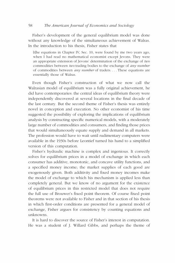
Imagine a cistern with a uniform thickness of unity, and with ashape shown in Figure 1.

The origin is placed at the northwest corner of the cistern, whichhas a vertical height of d units. For each 0 £ x £ d, the width of thecistern is given by the function f (x). If the cistern is filled with waterup to x units below the top of the cistern, the volume of water itcontains will be

Fisher designs the cistern so that the depth x is equal to the marginalutility, for that consumer and that good, of the volume of water itcontains, i.e.,

as an identity for all x. With this construction, the maximal depth dis equal to u¢(0), and one needs to select utility functions with a finitemarginal utility at zero in order to have cisterns of finite depth.Another feature of this utility function is that the consumer is satiated

xx

= ¢ ( )( )Úu f t dtd

f t dtd

( )Ú .x

¢uij

p x Yj ijj n

i i=Â £ = >( )

1

0,

.if l

x E piji m

j j=Â £ = >( )

1

0,

if and

¢ ( ) £ = >( )u x p xij ij i j ijl , if 0


when the cistern is filled to its top and consumption is equal to.

The connection between the utility function u(x) and the shape ofthe cistern f(x) is unusual, and the reader may find it useful to calculate f for various well-known utility functions. For example, ifu(x) = -e-x, the shape function is f(x) = 1/x, and the depth, d, is unity.

As a second example, if , the shape function is

f(x) = b and the box is rectangular. And finally if f(x) = b + at, withb + ad > 0, the utility function is given by

u xa

b ad bax b ad ax( ) = +( ) - - +( ) -( )( )1

122 6 2 42

3 2 3 2.

u x dxb

x( ) = -1

22

Ú ( )0d f t dt


0

d

Figure 1

A Cistern

In order to see a way in which these cisterns can be used to solvean optimization problem, consider a single consumer with utility function

Construct a cistern for each utility function uj(xj) and let their topsbe rigidly connected by a rod constrained to be horizontal, but freeto move vertically, so that the cisterns will float in a tub of waterwithout changing their relative positions. Insert a fixed amount ofwater, Y, into the right-most cistern, and let the interiors of the cis-terns be connected by rubber tubes so that the water flows easilyfrom one to another.

When the apparatus reaches an equilibrium, the input of water, Y,will be allocated among the n cisterns, with cistern j containing anamount xj. The level of water will be the same in each cistern, say lunits below the top, so that

We see that this assemblage of the Fisher cisterns solves the problem

max

,

u x

x Y

j j

j

( )=

ÂÂ

subject to

¢( ) =u x jj j l, .for each

x YjÂ = and

u x u xj j( ) = ( )Â .


I II III IV S C

#0

1

2

3

4

Figure 2

simply by using the fact that freely flowing water will seek a commonlevel in the series of interconnected cisterns, thereby equating themarginal utility for each good to a common price of unity.

We have evaluated the demand functions of this consumer atincome Y, and at prices p = (1, . . . , 1). In order to deal with generalprices, and several consumers, we shall have to assemble the cisternsin a considerably more complex fashion.

III

A Preliminary Machine: Pareto Optimal Allocations

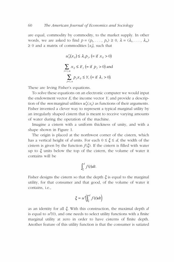
LET US CONSIDER a construction that is not quite the one used by Fisher,but that allows us to explore models of exchange with m consumers.Figure 3 depicts the case of two consumers (I, II) and two com-modities (A, B). Construct a separate rod for each of the m consumers.On the rod for the ith consumer, we place n cisterns, one for eachcommodity, and for each such good we connect all of the m cisternsreferring to that good by a tube in which water will flow. The westsides of the cisterns for each commodity are aligned parallel to a floatF lying on the surface of the water. The left end of each rod is attachedto this float, F. The i th rod will make an angle ai with the watersurface.

In this construction the float F is not permitted to move and theangles ai are fixed in advance. What does move are the cisterns alongeach rod; but in the following precisely constrained way.

Constraining the Cisterns

All of the cisterns relating to good j have their northwest corners atthe same horizontal distance, say pj, from their attachment to float F.

The distances from F may shift during the functioning of themachine but all distances relating to the same commodity are con-strained to be the same. These distances are determined by inserting,into the tube for good j, an amount of water equal to the marketsupply Ej of that good. The water levels for the m cisterns for goodj reach a common level, and together the cisterns move along therods so that this common level is equal to the water level in the


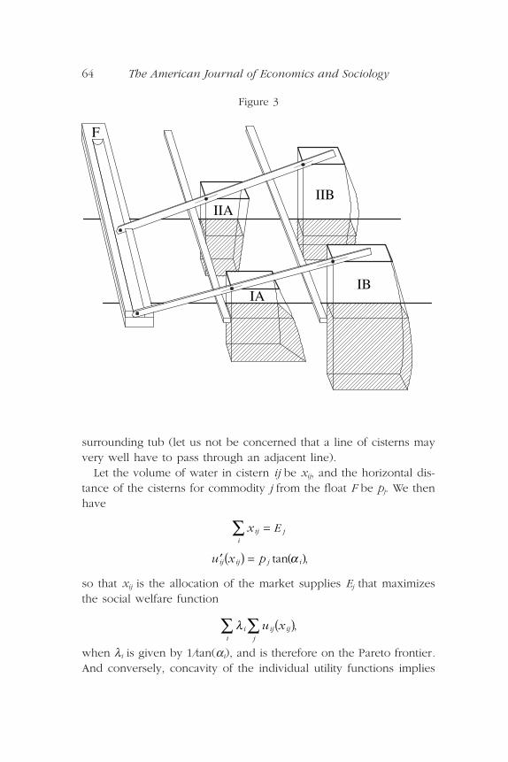
surrounding tub (let us not be concerned that a line of cisterns mayvery well have to pass through an adjacent line).

Let the volume of water in cistern ij be xij, and the horizontal dis-tance of the cisterns for commodity j from the float F be pj. We thenhave

so that xij is the allocation of the market supplies Ej that maximizesthe social welfare function

when li is given by 1/tan(ai), and is therefore on the Pareto frontier.And conversely, concavity of the individual utility functions implies

l ii

ij ijj

u xÂ Â ( ),

¢ ( ) = ( )u x pij ij j itan ,a

x Eij ji

=Â


F

IIAIIB

IBIA

Figure 3

that any Pareto optimal allocation is obtained by some selection ofli and therefore by some selection of these angles ai. Of course,Fisher wrote before Pareto and this concept does not appear in histhesis.

Typically this allocation will not satisfy the individual budget con-straints Spjxij = Yi and the angles of the rods must be systematicallyvaried so as to find those angles for which the value of consumptionequals income for each consumer. But at this point in our exposition,it is far from clear how to modify the apparatus so as to compareconsumption and income. Nothing in this machine permits us to cal-culate the cost of the commodity bundle demanded by a particularconsumer. At no place is a quantity multiplied by a price. We shallreturn to this issue after describing Fisher’s somewhat differentarrangement of these cisterns.

Fisher’s Construction (Preliminary)

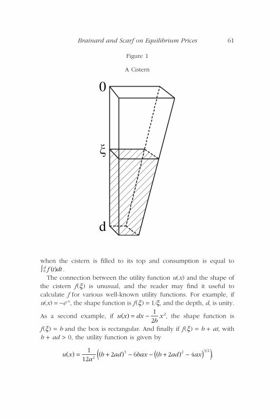
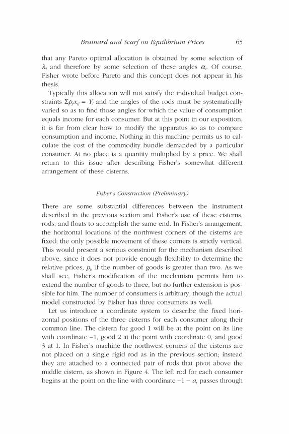
There are some substantial differences between the instrumentdescribed in the previous section and Fisher’s use of these cisterns,rods, and floats to accomplish the same end. In Fisher’s arrangement,the horizontal locations of the northwest corners of the cisterns arefixed; the only possible movement of these corners is strictly vertical.This would present a serious constraint for the mechanism describedabove, since it does not provide enough flexibility to determine therelative prices, pj, if the number of goods is greater than two. As weshall see, Fisher’s modification of the mechanism permits him toextend the number of goods to three, but no further extension is pos-sible for him. The number of consumers is arbitrary, though the actualmodel constructed by Fisher has three consumers as well.

Let us introduce a coordinate system to describe the fixed hori-zontal positions of the three cisterns for each consumer along theircommon line. The cistern for good 1 will be at the point on its linewith coordinate -1, good 2 at the point with coordinate 0, and good3 at 1. In Fisher’s machine the northwest corners of the cisterns arenot placed on a single rigid rod as in the previous section; insteadthey are attached to a connected pair of rods that pivot above themiddle cistern, as shown in Figure 4. The left rod for each consumerbegins at the point on the line with coordinate -1 - a, passes through


the corner of the cistern for good 1 at -1, and then through the cornerof the middle cistern for good 2 at 0. The right rod begins at the pointon the line with coordinate 1 + c, passes through the corner of thecistern for good 3 at 1, and then joins the left rod at the corner ofthe cistern for good 2.

The beginnings of these pairs of rods are secured on two floats,one to the left at coordinate -1 - a and the other to the right at coor-dinate 1 + c. The floats are permitted to move laterally, so that thevalues of a and c are arbitrary. Let us also assume for the momentthat the northwest corners of the cisterns describing the same good,for the various consumers, are all connected by a rigid bar parallelto the surface of the water, so that all of these corners are forced tobe at the same height. Movement of the floats implies sliding pivots.

As before, the cisterns for a common good are connected by tubingthrough which water will move freely. A quantity of water equal tothe supply of that good is entered into the corresponding tube bysetting the levels of certain plungers at the back of the tub. The waterlevels for the cisterns for each commodity will find a common level,and subsequently the floats to the right and left will move so that allof the cistern levels, for each consumer and for each good, will equil-ibrate at the water level of the tub. If the quantity of water in cistern


Figure 4

F

IIAIIB

IIC

IAIB

IC

F

ij is xij then Sixij = Ej for each good. Moreover, the surface of thewater in each cistern referring to good j is at the same depth belowits northwest corner, so that for each j the marginal utilities (xij) areidentical for all consumers i.

If we set pj = (xij) we see that the apparatus has found an allo-cation xij and prices p such that

As with the previous construction, the hydraulic instrument has produced a particular Pareto optimal allocation; in this case the allocation with the marginal utility of income equal to unity for allconsumers. Other Pareto optimal allocations can be found by multi-plying each utility function by a nonnegative constant, or by allow-ing the bars connecting the northwest corners of the cisterns to makean angle with the surface of the water different from zero.

But it is still not clear how to find an efficient allocation in whichthe value of consumption is equal to income for all consumers. Areasonable scholar might perfectly well have given up at this point,but Fisher persisted with an ingenious and intricate modification ofthe apparatus, designed to solve this problem.

It would be difficult to improve on Fisher’s description of the finalmechanism. The next section is taken directly from his thesis. Hedenotes the consumers by I, II, III and commodities by A, B, C. Hisstatements about marginal utilities and their relationship to prices areonly true at equilibrium.

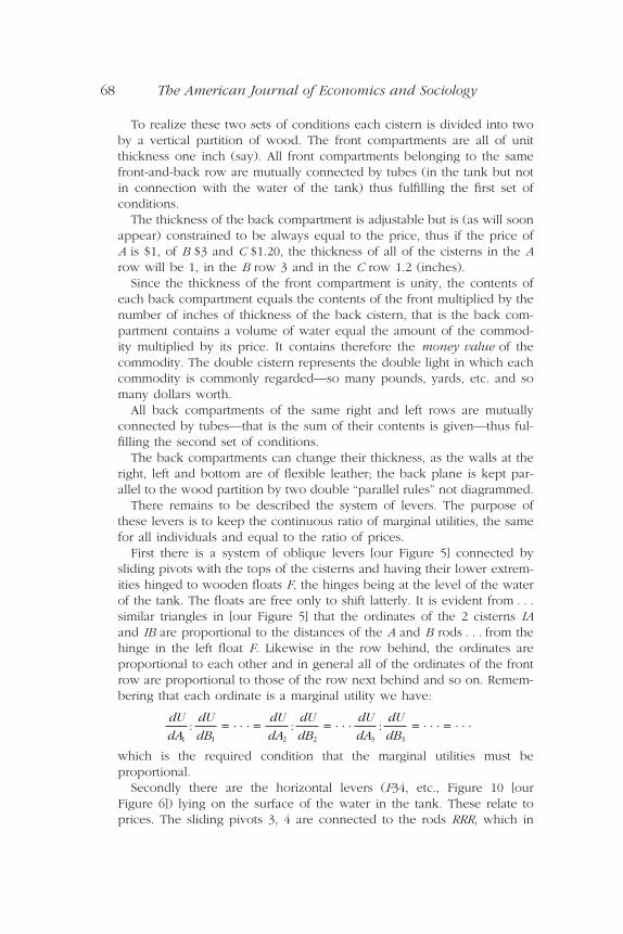
Fisher’s Construction (The Schematic Figure 5 and Text Taken from Section 4 of His Thesis)

The water in these cisterns must be subjected to two sets of conditions,first: the sum of all of the contents of IA, IIA, IIIA, etc., shall be a givenamount (vis: the whole of the commodity A consumed during the givenperiod) with a like given sum for the B row, C row, etc., secondly: thesum of IA, IB, IC, etc., each multiplied by a coefficient (the price of A, ofB, of C, etc.), shall be given (vis: the whole income of I during the period)with a like given sum for the II row, III row, etc.

¢ ( ) =u x pij ij j.

x Eij ji

=Â

¢uij

¢uij



To realize these two sets of conditions each cistern is divided into twoby a vertical partition of wood. The front compartments are all of unitthickness one inch (say). All front compartments belonging to the samefront-and-back row are mutually connected by tubes (in the tank but notin connection with the water of the tank) thus fulfilling the first set of conditions.

The thickness of the back compartment is adjustable but is (as will soonappear) constrained to be always equal to the price, thus if the price ofA is $1, of B $3 and C $1.20, the thickness of all of the cisterns in the Arow will be 1, in the B row 3 and in the C row 1.2 (inches).

Since the thickness of the front compartment is unity, the contents ofeach back compartment equals the contents of the front multiplied by thenumber of inches of thickness of the back cistern, that is the back com-partment contains a volume of water equal the amount of the commod-ity multiplied by its price. It contains therefore the money value of thecommodity. The double cistern represents the double light in which eachcommodity is commonly regarded—so many pounds, yards, etc. and somany dollars worth.

All back compartments of the same right and left rows are mutuallyconnected by tubes—that is the sum of their contents is given—thus ful-filling the second set of conditions.

The back compartments can change their thickness, as the walls at theright, left and bottom are of flexible leather; the back plane is kept par-allel to the wood partition by two double “parallel rules” not diagrammed.

There remains to be described the system of levers. The purpose ofthese levers is to keep the continuous ratio of marginal utilities, the samefor all individuals and equal to the ratio of prices.

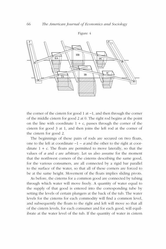
First there is a system of oblique levers [our Figure 5] connected bysliding pivots with the tops of the cisterns and having their lower extrem-ities hinged to wooden floats F, the hinges being at the level of the waterof the tank. The floats are free only to shift latterly. It is evident from . . .similar triangles in [our Figure 5] that the ordinates of the 2 cisterns IAand IB are proportional to the distances of the A and B rods . . . from thehinge in the left float F. Likewise in the row behind, the ordinates areproportional to each other and in general all of the ordinates of the frontrow are proportional to those of the row next behind and so on. Remem-bering that each ordinate is a marginal utility we have:

which is the required condition that the marginal utilities must be proportional.

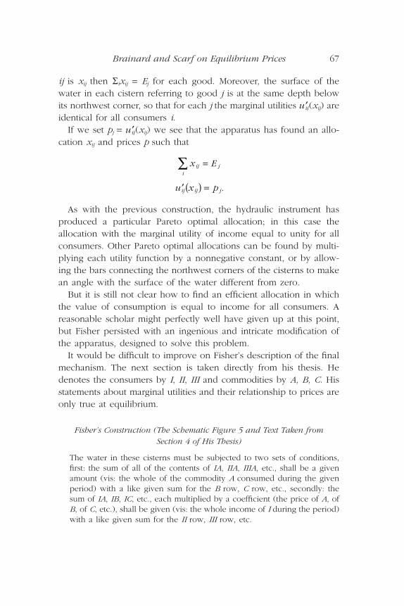
Secondly there are the horizontal levers (F34, etc., Figure 10 [our Figure 6]) lying on the surface of the water in the tank. These relate toprices. The sliding pivots 3, 4 are connected to the rods RRR, which in

dU

dA

dU

dB

dU

dA

dU

dB

dU

dA

dU

dB1 1 2 2 3 3

: : := ◊ ◊ ◊ = = ◊ ◊ ◊ = ◊ ◊ ◊ = ◊ ◊ ◊

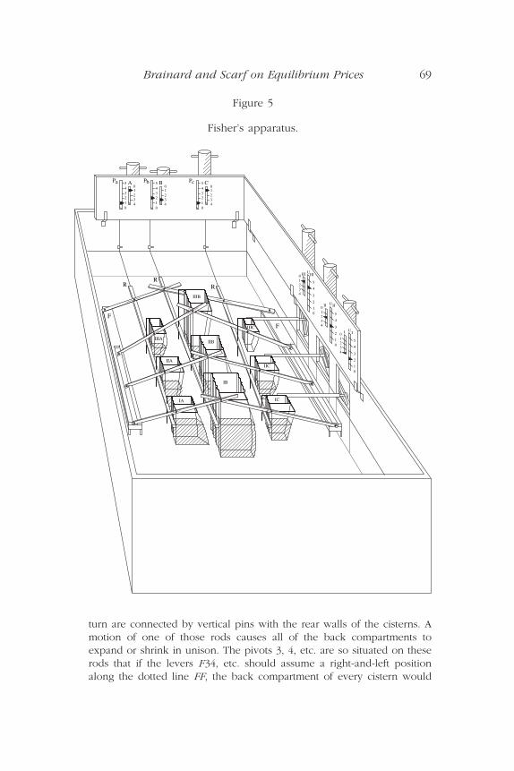
turn are connected by vertical pins with the rear walls of the cisterns. Amotion of one of those rods causes all of the back compartments toexpand or shrink in unison. The pivots 3, 4, etc. are so situated on theserods that if the levers F34, etc. should assume a right-and-left positionalong the dotted line FF, the back compartment of every cistern would


Figure 5

Fisher’s apparatus.

543210

1234

0P Aa

IA

IIA

IIIA

IIIB

IIB

IB

IC

IIC

5

4

3

2

10

UIIIIII0

1234

543210

1234

0P Bb

5

4

3

2

10

UIIII01234

5

4

3

2

10

UII

01234

RR

F

F

543210

1234

0P Cc

IIIC

R

be completely closed. Hence R3 equals the thickness of each back com-partment in th A row, R4 the corresponding thickness in the B row andso on.

By the similar triangles FR3 and F34 in Figure 10 [our Figure 6], it isclear that the lines R3 and R4, and consequently the rear thickness in theA and B rows are proportional to the distances of the A and B rods R andR from the float F. But we have just seen that the ordinates of IA and IBare proportional to these same distances. Hence the thickness of the back


3

4

F

IIIBIIIA IIIC

IIA IIB IIC

IA IB IC

F

R

R

R

Figure 6

compartments of the cisterns are proportional to the ordinates of thosecisterns, that is to marginal utilities. Hence we are free to call the thick-ness of each back compartment, the money price of the commodity towhich that cistern relates.

It is to be observed that the cisterns are free to move only vertically,the rods and rear cistern walls only forward and backward, the woodenfloats can shift sidewise right and left while the levers assume such posi-tions as the mechanism compels.

This ends our direct quotation from Fisher’s thesis, and his descrip-tion of his machine. In the next section, we describe our computersimulation of his model.

The Digital Version of the Fisher Machine

Did Fisher’s machine work? We knew it must have, at least after afashion, because Fisher reports that for 25 years he used his firstmodel in teaching. But we were curious to see it work, and couldnot help wondering whether the floats would come to rest againsttheir stops rather than in a “market” equilibrium. After some roman-tic thoughts about replicating the machine, tub, water, and all, wesettled on simulating the machine in Matlab. The physical features ofthe Fisher apparatus fall into two groups. The properties of the firstgroup—the quantity and expenditure cisterns and the system of rodscontrolling the elevations of the cisterns and the price dimension ofthe expenditure cisterns—determine the equilibrium prices and allo-cation, and when the system is out of equilibrium they determine theforces and pressures that move the rods, cisterns, floats, and bellowsthemselves. The second group of features—the tubes connecting thequantity and expenditure cisterns, the mass and surface area of the floats, the viscosity of water—govern the speed of adjustment ofthe system when it is out of equilibrium.

Our mathematical description of the first group of features isstraightforward and faithful to the hydraulic model, except for ignor-ing the actual model’s “imperfections”—the nonzero mass of the rodsand the thickness and mass of the walls of the cisterns. For any posi-tion of the consumer and price rods, we use Archimedes principleand the weight of water in each of the cisterns to calculate the vertical forces they exert; these forces are resolved into a rotational


force on each consumer’s rods, and a force inward or outward on thetwo floats. The inward or outward pressures on the price bellows ofeach consumer’s expenditure boxes are calculated from the differ-ence in the level of water inside and out of the expenditure cisterns.The resulting forces are transmitted to the price rods, and are alsoresolved into rotational forces and inward or outward forces on thefloats.

The construction of the Fisher model guarantees that in equilibriumor out, the quantity of water summed over each individual’s expen-diture cisterns always equals that individual’s money income, and thequantity of water, summed over an individual’s quantity cisterns,always equals the social endowment for each commodity. Tubesallow these fixed quantities to flow among the expenditure cisternsfor each individual, and among commodity cisterns across individu-als for each commodity. This preservation of quantities is easy tomimic in the Matlab version. As explained in the previous section byFisher, if the level of the water in each of the quantity and expendi-ture cisterns is the same as the level of water in the tub, each con-sumer will be maximizing utility subject to his or her budget constraintand the prices and allocations will correspond to a competitive equi-librium. This condition obviously implies that for each cistern, theArchimedes forces are exactly balanced by the weight of water in thecistern; in both the hydraulic and Matlab model, if the system is atrest in a competitive equilibrium, there are no net forces to disturbit. It is an intriguing question, whose answer we do not know,whether there are any rest points in which the level of water in thecisterns is different from the level in the tub.

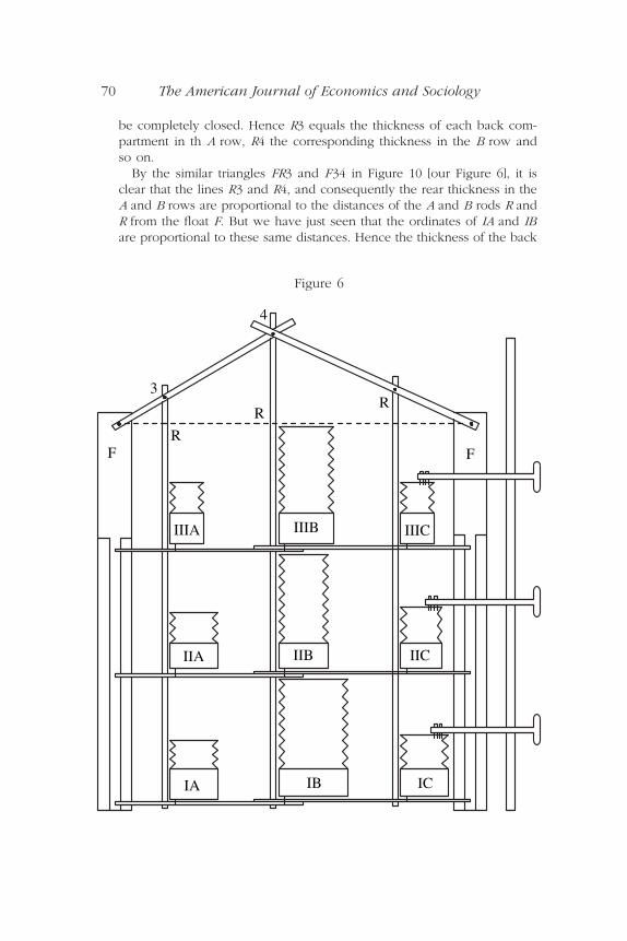
In contrast to its accurate description of the features of the hydraulicmodel determining equilibrium, the Matlab model is an approxima-tion of several features governing the dynamics of adjustment. Ratherthan the continuous, real-time, adjustments in the hydraulic machine,adjustments in the Matlab model are discrete, iteration by iteration.Three speeds of adjustment are crucial to the dynamics—the speedwith which water flows among cisterns, the speed with which thecisterns move up or down in the tub and the price bellows expandor contract, and the speed with which the pivot floats move in orout. The diameter, length, and surface characteristics of the tubes


used by Fisher to connect the cisterns are not known to us, nor are the mass, displacement, or surface area of the floats. If the dimen-sions of the tubes were known, textbook fluid mechanics could beused to calculate the flow as a function of pressure differentials, vis-cosity, surface frictions, etc.; those same textbooks suggest that as apractical matter, there is no substitute for estimating the flow exper-imentally. Similarly, while it might be theoretically possible to calcu-late how far in a moment of time a given force would move acistern—up or down—in the tub, as a function of its mass, shape, and surface areas, it would have been a daunting task. In our simu-lations, what is important are the relative speeds of adjustment. Ourintuition suggested that the vertical movements of the cisterns, theinward or outward movements of the floats, and the adjustment ofthe price bellows were likely to be much quicker than the adjust-ments of the fluid levels through the tubes. The results of a casualexperiment, using a one-liter coke bottle as a proxy for a cistern and a one-foot length of 5/8≤ hose for a tube, were consistent withthat intuition; a bottle of water two/thirds full came to a displacementequilibrium in a tub much faster (by a factor of something like 10)than when the same bottle was emptied into the tub by the hose.This led us to choose the parameters in the model so that the adjust-ments of the consumer rods, bellows, and floats are much more rapidthan the equalization of water levels in the commodity or expendi-ture cisterns.

Given these parameter choices, price and consumer rods adjust toalmost completely eliminate the net forces on them, while significantdifferences in the level of water in the various cisterns remain. Start-ing from an arbitrary initial condition, there is typically a rapid adjust-ment of rods and floats, followed by a much longer period duringwhich the water flows among the cisterns and the entire set of vari-ables move slowly together. In our actual simulations it does notappear that the stability of the adjustment mechanism is much affectedby the precise values of these parameters, so long as the step size,corresponding to an iteration, is kept small. As will be seen, theadjustment paths display this qualitative behavior; from an initial dis-equilibrium of both prices and quantities, prices adjust rapidly tolevels that balance the forces on the rods, followed by much slower


adjustment as the water flows between cisterns. The Matlab modelalso ignores two physical phenomena that could, in principle, beimportant to the dynamics of adjustment—the increase in drag thatresults from increases in velocity, and inertia. Inertia could, even withcontinuous time, result in overshooting, with damped oscillations ofthe system, around equilibrium values. The equations used in theMatLab program are found in the Appendix.

Fisher’s Use of the Machine

Fisher regarded his model as “the physical analogue of the ideal eco-nomic market” (Mathematical investigations, p. 44), with the virtuethat “[t]he elements which contribute to the determination of pricesare represented each with its appropriate role and open to the scrutinyof the eye . . .” providing “a clear and analytical picture of the inter-dependence of the many elements in the causation of prices.” Fisheralso saw the machine as way of demonstrating comparative staticsresults “to employ the mechanism as an instrument of investigationand by it, study some complicated variations which could scarcely besuccessfully followed without its aid.” We do not know how trans-parent the model was to Fisher’s students, but it is easy to imaginethe excitement they may have felt in watching the model at work,accompanied by enthusiastic commentary by Fisher.

In principle the Fisher model will find the competitive equilibriumfor any three-commodity, three-person exchange economy with addi-tively separable preferences, with the restriction that individuals’endowments are some fraction of the aggregate commodity endow-ment bundle—a restriction implicit in the assumption that individ-uals are endowed with fixed money incomes rather than arbitrarybundles of commodities. To find a particular equilibrium merelyrequires specifying the shapes of the 3 ¥ 3 cisterns, and prescribingthe aggregate supplies and individual endowments. As previouslyexplained, for the Fisher machine to work, the preferences and quan-tity endowments must be assigned to rows so that in equilibrium thecommodity in the middle row has the highest marginal utility. Givenpreferences and initial quantities, comparative static results can beobtained simply by altering the aggregate supplies or individual


endowments as desired and observing the new equilibrium prices andallocation.

Although we do not know what experiments Fisher actually ranwith his machine, he does describe eight comparative static exercises.Some of these illustrate basic features of the system, for example, thatproportional increases in money incomes result in an equal propor-tional increase in each price, with no change in the allocation ofgoods. Another simple exercise discussed by Fisher examines whetherproportional increases in the endowment of goods necessarily resultin proportional decreases in prices, as was apparently, and incorrectly,believed by Mill. Some exercises illustrate less intuitive properties ofexchange economies: increasing one individual’s income may makesome other individual better off and also the possibility of “immiser-ating growth,” i.e., increasing an individual’s endowment of a goodmay actually lower his or her welfare.

Although Fisher discusses the way in which changing an individ-ual’s preferences alters the equilibrium, it was expensive to changethe cisterns in his model and it seems unlikely they were changedafter some initial experimentation. The cisterns in Fisher’s original1893 model included a fairly rich variety of shapes; the cisterns in his1925 model look like they may all have rectangular faces, corre-sponding to quadratic utility functions. While Fisher’s constructionmade it difficult to vary preferences, his set up made it easy to changequantities; by simply moving a plunger for a commodity or individ-ual’s income he could force more water into the associated columnor row of cisterns.

Dynamics of the Machine

We used our Matlab representation of the hydraulic machine to sim-ulate the path of adjustment for a variety of preferences, endowments,and initial conditions. We do not have a basis for comparison withFisher’s actual model; Fisher does not analyze or describe the dynamicbehavior of his machine.

It is easy to imagine that, as Fisher slowly depressed a quantityplunger to change the equilibrium, the flows of water between cis-terns and the movements of lever arms were rapid enough to keep


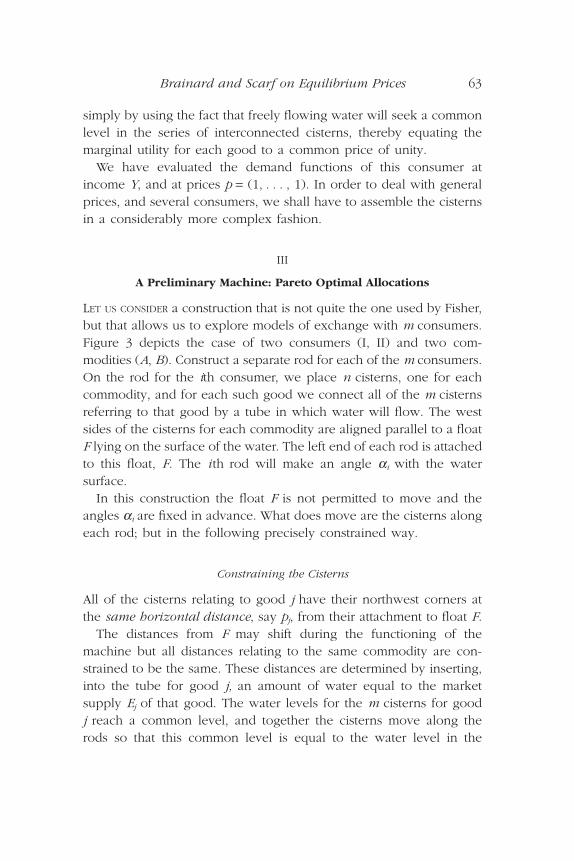
the system in the neighborhood of the shifting equilibrium; it is likelythat in Fisher’s experiments the initial conditions were never very farfrom equilibrium. In contrast, in our simulations we typically startedthe system with arbitrary allocations of the quantities to the cisterns(dividing the quantities equally across individuals and expendituresby individuals equally across commodities) and arbitrary prices. As a consequence our simulations show rapid movements of prices early in the adjustment process, with substantial discrepanciesbetween the quantity of a commodity j being allocated to individuali, q[i, j ] and the quantity of that good that could be purchased by the allocation of expenditures on commodity j by individual i, qe [i, j ], given current prices. These characteristics are evident inthree examples given in Figure 5, which display paths of prices, andthese discrepancies for the first commodity (q [i, 1] - qe [i, 1]) duringthe adjustment process.

It is difficult to imagine an economic interpretation of Fisher’sadjustment process. Throughout the adjustment process individuals’commodity allocations sum to the social endowment, and each individual’s money income is exactly exhausted in that individual’sexpenditure cisterns. However, allocations are not on the contractcurve (ratios of marginal utilities are not the same across individuals),individuals are not maximizing utility (the ratios of the marginal util-ities of the quantities being consumed by an individual are not thesame as the ratios of prices), and the value at current prices of a goodallocated to an individual is typically not equal to the nominal incomeallocated to purchase that good by the individual (the water level inthe front and back cisterns for a given commodity need not be equal).

An Example of Multiple Equilibria

The restrictive assumptions on preferences and endowments embod-ied in the Fisher machine are not sufficient to guarantee uniqueness.Indeed it is possible to have multiple equilibria even if the additivelyseparable preferences are restricted to be quadratic. How would themachine behave if in fact there is more than one equilibrium? A com-bination of preferences and endowments that gives rise to multipleequilibria is specified in the following example.


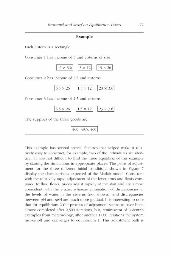
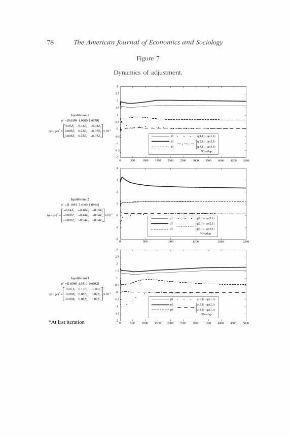
This example has several special features that helped make it rela-tively easy to construct, for example, two of the individuals are iden-tical. It was not difficult to find the three equilibria of this exampleby starting the simulations in appropriate places. The paths of adjust-ment for the three different initial conditions shown in Figure 7display the characteristics expected of the Matlab model. Consistentwith the relatively rapid adjustment of the lever arms and floats com-pared to fluid flows, prices adjust rapidly at the start and are almostcoincident with the y axis, whereas elimination of discrepancies inthe levels of water in the cisterns (not shown), and discrepanciesbetween q [·] and qe [·] are much more gradual. It is interesting to notethat for equilibrium 2 the process of adjustment seems to have beenalmost completed after 2,500 iterations, but, reminiscent of Lorentz’sexamples from meteorology, after another 1,000 iterations the systemmoves off and converges to equilibrium 1. This adjustment path is


Example

Each cistern is a rectangle.

Consumer 1 has income of 5 and cisterns of size:

Consumer 2 has income of 2.5 and cisterns:

Consumer 3 has income of 2.5 and cisterns:

The supplies of the three goods are:

400, 49.5, 400

23 ¥ 3.61.5 ¥ 126.5 ¥ 26

23 ¥ 3.61.5 ¥ 126.5 ¥ 26

13 ¥ 263 ¥ 1246 ¥ 3.6


3

2.5

2

1.5

1

0.5

0

-0.5

-1

-1.5

-20 500 1000 1500 2000 2500 3000 3500 4000 4500 5000

0 500 1000 1500 2000 2500 3000 3500 4000 4500 5000

3

2.5

2

1.5

1

0.5

0

-0.5

-1

-1.5

-2

4

2

1

0

-1

-20 500 1000 1500 2000 2500

3

p1

p2

p3 q(3,1) - qe(3,1)

q(2,1) - qe(2,1)

q(1,1) - qe(1,1)

*Overlap

p1

p2

p3 q(3,1) - qe(3,1)

q(2,1) - qe(2,1)

q(1,1) - qe(1,1)

*Overlap

p1

p2

p3 q(3,1) - qe(3,1)

q(2,1) - qe(2,1)

q(1,1) - qe(1,1)

*Overlap

*

1 2 3* 2

1 2 3

1 2 3

Equilibrium 3

[1.6560 1.9310 0.6082]

0.07 0.13 0.00

( ) 0.00 0.08 0.02 10

0.00 0.08 0.02

p

E E E

q qe E E E

E E E

−

=− −

− = − ×

−

*

1 2 3* 2

1 2 3

1 2 3

Equilibrium 1

[0.6199 1.9600 1.6370]

0.03 0.44 0.04

( ) 0.005 0.22 0.07 10

0.005 0.22 0.07

p

E E E

q qe E E EE E E

−

=−

− = − ¥−

*

1 2 3* 2

1 2 3

1 2 3

Equilibrium 2

[1.1054 2.4060 1.0964]

0.14 0.10 0.05

( ) 0.005 0.44 0.04 10

0.005 0.04 0.04

p

E E E

q qe E E E

E E E

−

=− − −

− = − − − ×

− − −

*At last iteration

Figure 7

Dynamics of adjustment.

shown in Figure 8. Since we do not have an economic interpretationof the dynamics of adjustment in the hydraulic model, we cannotmake use of the usual economic propositions about the equilibria,for example, the role of the assumption of gross substitutability inguaranteeing uniqueness of the competitive equilibrium and stabilityof the Walrasian price adjustment mechanism.

Appendix

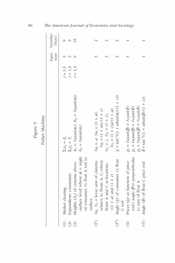
The equations used in the digital version of the Fisher machine aregiven in Figure 9. The state of the system is given by the values of24 state variables—the nine commodity and nine expenditure alloca-tions (xij, yij), two float locations (a, c), three consumer rod angles


0 2000 4000 6000 8000 10000 12000-2

-1

0

1

2

3

4Equilibrium 2 (12,000 iterations)

p1

p2

p3 q(3,1) - qe(3,1)

q(1,1) - qe(1,1)

*Overlap

q(2,1) - qe(2,1)

Figure 8


Figu

re 9

Fish

er M

achin

e

Equa-

Var

iable

stio

ns

(New

)

(1)

Mar

ket

clea

ring

S ix i

j=

Ej

j=

1,3

39

(2)

Exp

enditu

re c

onst

rain

tsS i

y ij

=Y

ii

=1,

33

9(3

)H

eigh

ts (

hij)

of

cist

erns

above

h

i1=

a1tan

(ai);

hi2

=a

2tan

(ai);

i=

1,3

915

surf

ace

leve

l w

her

e a i

=an

gle

hi3

=a

3tan

(ai)

of

consu

mer

i’s fl

oat

A r

od t

o

surf

ace

(3¢)

ai,

c i=

leve

r ar

m o

f ci

ster

ns

a1

=a,

a2

=(1

+a),

32

rela

tive

to fl

oat

s A,

Ciw

her

e a

3=

(1 +

a)c

/(1

+c)

float

s A a

nd C

at

loca

tions

c 1=

c,

c 2=

(1 +

c),

33

-(1

+a)

and (

1 +

c)c 3

=(1

+c)

a/(

1 +

a)

(3≤)

Angl

e (g

i) o

f co

nsu

mer

i’s fl

oat

g i

=ta

n-1((

1 +

a)tan

(ai)/(

1 +

c))

33

C r

od

(4)

Price

s (p

j) as

funct

ion o

f price

p 1

=a

1tan

(b)

=c 3

tan(d

)3

4ro

d’s a

ngl

e b

to p

erpen

dic

ula

r p 2

= a

2tan

(b)

=c 2

tan(d

)to

axi

s of

float

Ap 3

=a

3tan

(b)

=c 1

tan(d

)(4

¢)Angl

e (d

) of

float

C p

rice

rod

d=

tan

-1((

1 +

a)tan

(b)/

(1 +

c))

11

ll

ll

ll

l

ll

l

ll

ll

l

ll


(5)

Mar

ginal

util

ities

of

com

modity

(D

ij-

x ij)

=(x

ij)

99

allo

catio

n(6

)M

argi

nal

util

ities

of

expen

ditu

re

(Dij

- y

ij)

=(y

ij/p

j)9

9al

loca

tion w

her

e x i

j, y

ij=

dep

th o

f w

ater

in

com

modity

, ex

pen

ditu

re

cist

ern;

Dij

=m

axim

um

dep

th o

f ci

ster

n(7

)Chan

ge i

n a

ngl

es o

f co

nsu

mer

s’

Dai

=S a

/((1

+ta

n(a

i)2 )S j

)i

=1,

33

–ro

ds

(a f

unct

ion o

f w

eigh

t of

¥S j

aj[x

ij-

(hij)

+undis

pla

ced w

ater

in c

iste

rn)

y ij-

p j(h

ij)]

wher

e s a

=sp

eed o

f ad

just

men

t(8

)ch

ange

in p

rice

rod a

ngl

e Db

=S b

/((1

+ta

n(b

)2 )S j

)1

–(f

unct

ion o

f pre

ssure

s on

¥S j

S i[

ajp

r ij(

yij,

hij)]

price

bel

low

s) w

her

e s b

=sp

eed o

f ad

just

men

t(8

¢)pr

ij(y

ij,

hij)

=pre

ssure

on p

rice

pr

ij(y

ij, h

ij)

=tf

(t)d

tbel

low

s ij

wher

e f(

t) =

wid

th

of

cist

ern a

t dep

th t

Ú-

-(

)0y

ijij

ijD

h

l

aj2

l

uiji-

1

uiji-

1l

aj2

l

¢u

ij¢u

ij


(9)

Chan

ge i

n fl

oat

loca

tions

Da=

-Sa/(

1 +

a)S

i{tan

(ai)(x

i1-

(hi1)

2–

(chan

ge i

n r

elat

ive

price

s)+

y i1

- p 1

(hi1))

- ta

n(b

)pri

1(y

i1,

hi1)}

Dc=

-Sc/(

1 +

c)S i

{tan(g

i)(x

i3-

(hi3)

+y i

3-

p 3(h

i3))

-

tan(d

)pr i

3(y

i3,

hi3)}

(10)

Quan

tity

adju

stm

ents

(S x

=flow

Dx

1j=

S x(x

2j-

x 1i) +

S x(x

3j-

x 1j)

j=1

,36

–as

funct

ion

of

pre

ssure

Dx

2j=

S x(x

1j-

x 2i) +

S x(x

3j-

x 2j)

diffe

rentia

l)Dx

3j=

S x(x

1j-

x 3i) +

S x(x

2j-

x 3j)

(11)

Exp

enditu

re a

dju

stm

ents

Dy1j

=S x

(y2j

- y

1i)

+ S x

(y3j

- y

1j)

j=

1,3

6–

Dy2j

=S x

(y1j

- y

2i)

+S x

(y3j

- y

2j)

Dy3j

=S x

(y1j

- y

3i)

+S x

(y2j

- y

3j)

6464

uii 3

1-u

ii 31-

uii 1

1-u

ii 11-

Figu

re 9

Con

tin

ued

Equa-

Var

iable

stio

ns

(New

)

(ai), and a single price rod angle (b). Together these 24 variablesdetermine 40 other variables used in the solution of the model. Thesets of equations in (1) through (6) give the constraints and relation-ships among these variables. The condition that the commodity andexpenditure allocations add up to the exogenous commodities andincomes (Ej, Yi) are given by six equations in (1) and (2). Not count-ing these equations there are 18 independent equations and variables.The equations in (3) give the heights of the cisterns above the surfaceof the water (hij) as determined by the lever arms laj, lcj implied bythe float locations and consumer rod angles (ai). Equations in (4) giveprices as a function of the same lever arms and the price rod angle(b). Equations (5) and (6) give the depth of water in the commodityand expenditure cisterns (xij, Yij) implied by the commodity andexpenditure allocations.

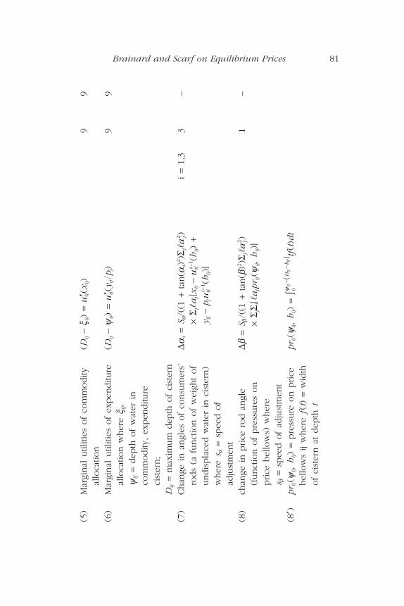
In equilibrium the heights for the cisterns above the surface of thewater in the tub (hij), the marginal utilities implied by the commod-ity allocations ( (xij)) and the marginal utilities implied by the expen-diture allocations ( (yij /pj)) are all equal and proportional to theprices.

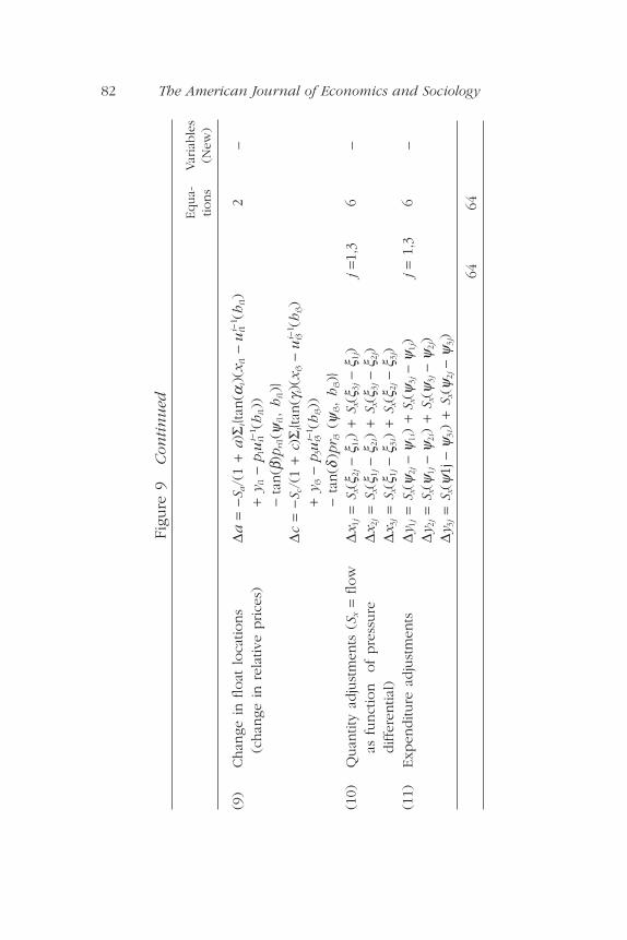
Equations (7) through (11) give the adjustment of the 24 state vari-ables iteration by iteration as a function of the forces on the rods andfloats when the system is out of equilibrium. (For economy of pres-entation and computation the adjustments of a and c assume that themoments of the consumer rods are zero, equivalently that the (ai)and (b) are changing so slowly that the motion of the cisterns throughthe water induces neglible resistance.)

¢uij

¢uij


Documents

How to Compute Equilibrium Prices in 1891 - Yale Universitydido.econ.yale.edu/~hes/pub/how-to-compute.pdf · How to Compute Equilibrium Prices in 1891 By WILLIAM C. BRAINARD and HERBERT