How to improve international competitiveness of Portuguese ... · How to improve international competitiveness of Portuguese economy ... 5See Silberberg and Suen (2001) for speci–c

How to improve international competitiveness ofPortuguese economy�

Elsa Cristina Neves Januário Vazy

(draft version: please do not quote)

1 September 2006(ETSG Conference - 2006)

Contents

1 Introduction 2

2 Static General Equilibrium Model for Portugal 22.1 Firm Behaviour and Foreign Trade . . . . . . . . . . . . . . . . . 3

2.1.1 How to Produce? . . . . . . . . . . . . . . . . . . . . . . . 42.1.2 Productivity of primary factors . . . . . . . . . . . . . . . 72.1.3 How much to Produce? . . . . . . . . . . . . . . . . . . . 82.1.4 International trade as a connection between economies . . 11

2.2 The Behaviour of the representative family . . . . . . . . . . . . 132.3 Government Behaviour . . . . . . . . . . . . . . . . . . . . . . . . 152.4 Investment Demand . . . . . . . . . . . . . . . . . . . . . . . . . 162.5 General equilibrium in the economy . . . . . . . . . . . . . . . . 172.6 Data base . . . . . . . . . . . . . . . . . . . . . . . . . . . . . . . 18

3 Alternative Scenarios and Results 19

A Used Aggregation 25

B Variables List 27B.1 Endogenous variables . . . . . . . . . . . . . . . . . . . . . . . . . 27B.2 Exogenous variables . . . . . . . . . . . . . . . . . . . . . . . . . 27B.3 Parameters . . . . . . . . . . . . . . . . . . . . . . . . . . . . . . 28

C Equation list 29�With �nancial support of CEFAG�UE, "Centro de Estudos e Formação Avançada em

Gestão" of University of Évora. I am grateful with the important contribution made byRenato Flores and Luis Costa.

yUniversity of Évora, Economics Department ([email protected]).

1

1 Introduction

Last developments of European process of integration, as the enlargement toeast, created new questions related to the Portuguese economy performanceand is future development. Many politicians have been saying that Portuguese�rms must be more competitive in international markets, especially now thatnew member-states have the same accessibility to the European market thanPortugal and some advantages on the attraction of new investments. It hasbeen said also that the improvement of Portuguese economy is only possibleif labour become more productive. Thus, the improvement of productivity inPortugal is being considered one important key issue to future success of theeconomy.In this work we do not pretend to study how to improve the productivity,

or which policy should be adopted by government, or even which incentiveshould be given to Portuguese �rms. Instead, it is our aims to identify the typeof labour (skilled or unskilled) which productivity should be improved and inwhich sectors should that happen.The importance of these questions relates to the costs of productivity im-

provements and also to the diverse importance of di¤erent sectors on exports.Thus, it is expected that the same increase in productivity, but in di¤erentsectors, will lead to di¤erent e¤ects on the improvement of exports and tradebalance.

2 Static General Equilibrium Model for Portu-gal

The aim of this framework is to model the Portuguese economy. To this end weconsider 5 agents and 2 markets. Foreign currencies are not considered becausedata are expressed in the same monetary unit.

Table 1: Agents and marketsAgents MarketsFamilies GoodsFirms Factors

Banks (Investment)Government

Rest of the World

The adopted aggregation used for sectors is that used in Brucker (1998), inhis classi�cation of competitiveness factors.1

Table 2: Sectors of activity

1See appendix A with the relationship between the GTAP Data Base and the Brucker(1998) proposal.

2

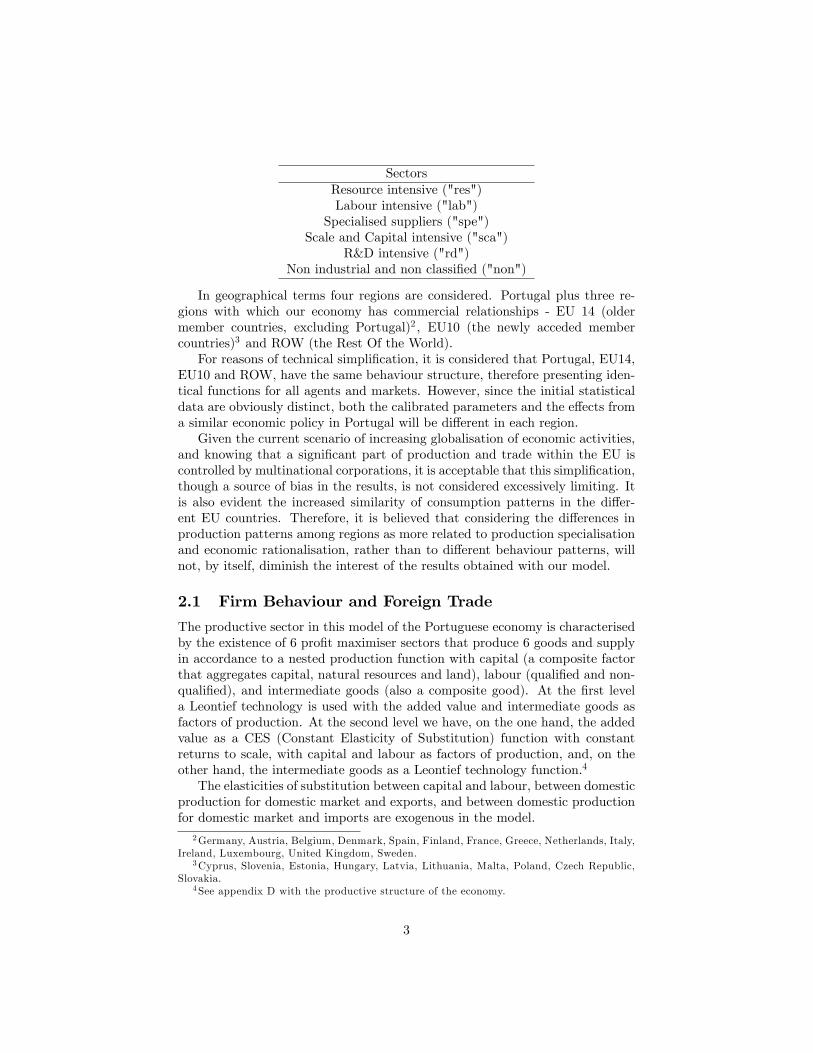
SectorsResource intensive ("res")Labour intensive ("lab")

Specialised suppliers ("spe")Scale and Capital intensive ("sca")

R&D intensive ("rd")Non industrial and non classi�ed ("non")

In geographical terms four regions are considered. Portugal plus three re-gions with which our economy has commercial relationships - EU 14 (oldermember countries, excluding Portugal)2 , EU10 (the newly acceded membercountries)3 and ROW (the Rest Of the World).For reasons of technical simpli�cation, it is considered that Portugal, EU14,

EU10 and ROW, have the same behaviour structure, therefore presenting iden-tical functions for all agents and markets. However, since the initial statisticaldata are obviously distinct, both the calibrated parameters and the e¤ects froma similar economic policy in Portugal will be di¤erent in each region.Given the current scenario of increasing globalisation of economic activities,

and knowing that a signi�cant part of production and trade within the EU iscontrolled by multinational corporations, it is acceptable that this simpli�cation,though a source of bias in the results, is not considered excessively limiting. Itis also evident the increased similarity of consumption patterns in the di¤er-ent EU countries. Therefore, it is believed that considering the di¤erences inproduction patterns among regions as more related to production specialisationand economic rationalisation, rather than to di¤erent behaviour patterns, willnot, by itself, diminish the interest of the results obtained with our model.

2.1 Firm Behaviour and Foreign Trade

The productive sector in this model of the Portuguese economy is characterisedby the existence of 6 pro�t maximiser sectors that produce 6 goods and supplyin accordance to a nested production function with capital (a composite factorthat aggregates capital, natural resources and land), labour (quali�ed and non-quali�ed), and intermediate goods (also a composite good). At the �rst levela Leontief technology is used with the added value and intermediate goods asfactors of production. At the second level we have, on the one hand, the addedvalue as a CES (Constant Elasticity of Substitution) function with constantreturns to scale, with capital and labour as factors of production, and, on theother hand, the intermediate goods as a Leontief technology function.4

The elasticities of substitution between capital and labour, between domesticproduction for domestic market and exports, and between domestic productionfor domestic market and imports are exogenous in the model.

2Germany, Austria, Belgium, Denmark, Spain, Finland, France, Greece, Netherlands, Italy,Ireland, Luxembourg, United Kingdom, Sweden.

3Cyprus, Slovenia, Estonia, Hungary, Latvia, Lithuania, Malta, Poland, Czech Republic,Slovakia.

4See appendix D with the productive structure of the economy.

3

Returns on capital and wages are equal across sectors since it is consideredthat there is perfect domestic factors�mobility.Firms pay taxes for the use of resources (capital and labour) as well as for

the use of intermediate goods.The behaviour of each �rm may be generalised in two groups of decisions on

how and how much to produce. In the �rst group the producer should choosethe optimal combination of primary and intermediate resources that are neededto produce, i.e. the best way of obtaining goods or services. At the second groupthe agent�s decisions determine how much will be distributed in the domesticmarket along with imported goods, and how much will go to the foreign market,i.e. the optimum level of production.

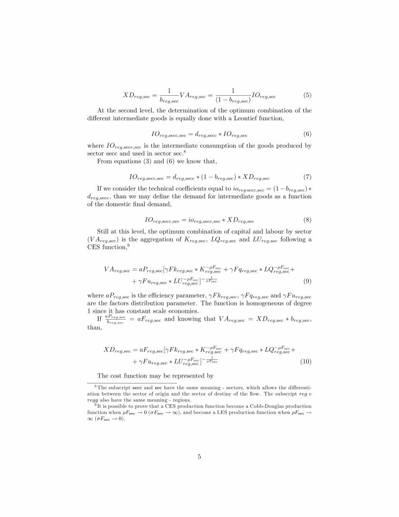
2.1.1 How to Produce?

At a �rst level the �rm chooses the basket of intermediate goods and the basketof primary factors by means of a Leontief production function. This type offunction assumes that the production of each sector is done with minimum �xedamounts from the baskets of intermediate goods and factors of production, i.e.�xed coe¢ cients. This mean that it is not possible the substitution betweenthem, i.e. is not possible to produce only with intermediate goods or only withprimary factors, since they are perfect complementary in this function.5

At this level the generic production function (g), where XDreg;sec is thedomestic production,6 V Areg;sec is the value added by each sector (or the basketof capital and labour necessary in each sector) and IOreg;sec is the basket ofintermediate goods used by each sector.7

XDreg;sec = g (V Areg;sec; IOreg;sec) (1)

Both V Areg;sec and IOreg;sec are �xed parts of XDreg;sec,

V Areg;sec = breg;sec �XDreg;sec (2)

IOreg;sec = (1� breg;sec) �XDreg;sec (3)

where breg;sec is the �xed coe¢ cients that relates the basket of productive factorswith the production, in each region. Therefore, XDreg;sec can been written as

XDreg;sec = min

�1

breg;secV Areg;sec;

1

(1� breg;sec)IOreg;sec

�(4)

The cost minimisation implicit in the rational behaviour of the producer allowsthe presentation of the former equation in the following way,

5See Silberberg and Suen (2001) for speci�c issues about Leontief and CES functions .6The subscript "reg" and "sec" means that the variable is disaggregated by regions and

sectors.7We can consider V Areg;sec and IOreg;sec as generic functions with distinct factors of

production, V Areg;sec = f(Kreg;sec; Lreg;sec) and IOreg;sec = z(Xreg;secc;sec), respectively.

4

XDreg;sec =1

breg;secV Areg;sec =

1

(1� breg;sec)IOreg;sec (5)

At the second level, the determination of the optimum combination of thedi¤erent intermediate goods is equally done with a Leontief function,

IOreg;secc;sec = dreg;secc � IOreg;sec (6)

where IOreg;secc;sec is the intermediate consumption of the goods produced bysector secc and used in sector sec.8

From equations (3) and (6) we know that,

IOreg;secc;sec = dreg;secc � (1� breg;sec) �XDreg;sec (7)

If we consider the technical coe¢ cients equal to ioreg secc;sec = (1� breg;sec)�dreg;secc, than we may de�ne the demand for intermediate goods as a functionof the domestic �nal demand,

IOreg;secc;sec = ioreg;secc;sec �XDreg;sec (8)

Still at this level, the optimum combination of capital and labour by sector(V Areg;sec) is the aggregation of Kreg;sec, LQreg;sec and LUreg;sec following aCES function,9

V Areg;sec = aPreg;sec[ Fkreg;sec �K��Fsecreg;sec + Fqreg;sec � LQ��Fsecreg;sec+

+ Fureg;sec � LU��Fsecreg;sec ]� 1�Fsec (9)

where aPreg;sec is the e¢ ciency parameter, Fkreg;sec, Fqreg;sec and Fureg;secare the factors distribution parameter. The function is homogeneous of degree1 since it has constant scale economies.If aPreg;sec

breg;sec= aFreg;sec and knowing that V Areg;sec = XDreg;sec � breg;sec,

than,

XDreg;sec = aFreg;sec[ Fkreg;sec �K��Fsecreg;sec + Fqreg;sec � LQ��Fsecreg;sec+

+ Fureg;sec � LU��Fsecreg;sec ]� 1�Fsec (10)

The cost function may be represented by

8The subscript secc and sec have the same meaning - sectors, which allows the di¤erenti-ation between the sector of origin and the sector of destiny of the �ow. The subscript reg eregg also have the same meaning - regions.

9 It is possible to prove that a CES production function become a Cobb-Douglas productionfunction when �Fsec ! 0 (�Fsec !1), and become a LES production function when �Fsec !1 (�Fsec ! 0).

5

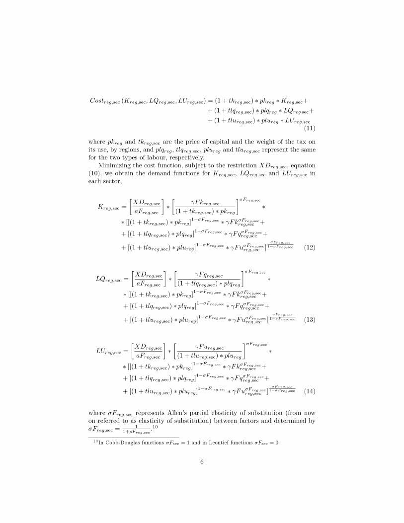
Costreg;sec (Kreg;sec; LQreg;sec; LUreg;sec) = (1 + tkreg;sec) � pkreg �Kreg;sec+

+ (1 + tlqreg;sec) � plqreg � LQreg sec++ (1 + tlureg;sec) � plureg � LUreg;sec

(11)

where pkreg and tkreg;sec are the price of capital and the weight of the tax onits use, by regions, and plqreg, tlqreg;sec, plureg and tlureg;sec represent the samefor the two types of labour, respectively.Minimizing the cost function, subject to the restriction XDreg;sec, equation

(10), we obtain the demand functions for Kreg;sec, LQreg;sec and LUreg;sec ineach sector,

Kreg;sec =

�XDreg;secaFreg;sec

��

Fkreg;sec(1 + tkreg;sec) � pkreg

��Freg;sec�

� [[(1 + tkreg;sec) � pkreg]1��Freg;sec � Fk�Freg;secreg;sec +

+ [(1 + tlqreg;sec) � plqreg]1��Freg;sec � Fq�Freg;secreg;sec +

+ [(1 + tlureg;sec) � plureg]1��Freg;sec � Fu�Freg;secreg;sec ]�Freg;sec

1��Freg;sec (12)

LQreg;sec =


��

Fqreg;sec(1 + tlqreg;sec) � plqreg

��Freg;sec�





LUreg;sec =


��

Fureg;sec(1 + tlureg;sec) � plureg

��Freg;sec�





where �Freg;sec represents Allen�s partial elasticity of substitution (from nowon referred to as elasticity of substitution) between factors and determined by�Freg;sec =

11+�Freg;sec

.10

10 In Cobb-Douglas functions �Fsec = 1 and in Leontief functions �Fsec = 0.

6

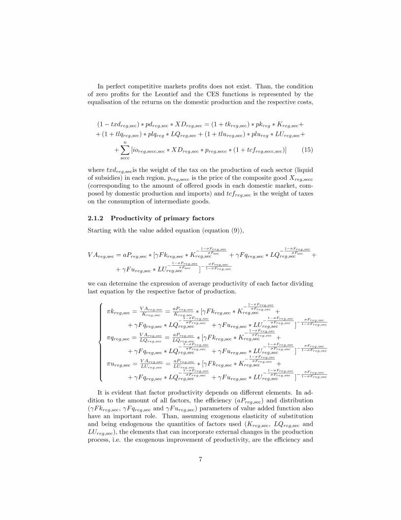
In perfect competitive markets pro�ts does not exist. Than, the conditionof zero pro�ts for the Leontief and the CES functions is represented by theequalisation of the returns on the domestic production and the respective costs,

(1� txdreg;sec) � pdreg;sec �XDreg;sec = (1 + tkreg;sec) � pkreg �Kreg;sec+

+(1 + tlqreg;sec) � plqreg � LQreg;sec + (1 + tlureg;sec) � plureg � LUreg;sec+

+nXsecc

[ioreg;secc;sec �XDreg;sec � preg;secc � (1 + tcfreg;secc;sec)] (15)

where txdreg;secis the weight of the tax on the production of each sector (liquidof subsidies) in each region, preg;secc is the price of the composite good Xreg;secc(corresponding to the amount of o¤ered goods in each domestic market, com-posed by domestic production and imports) and tcfreg;sec is the weight of taxeson the consumption of intermediate goods.

2.1.2 Productivity of primary factors

Starting with the value added equation (equation (9)),

V Areg;sec = aPreg;sec � [ Fkreg;sec �K� 1��Freg;sec

�Fsecreg;sec + Fqreg;sec � LQ

� 1��Freg;sec�Fsec

reg;sec +

+ Fureg;sec � LU� 1��Freg;sec

�Fsecreg;sec ]

� �Freg;sec1��Freg;sec

we can determine the expression of average productivity of each factor dividinglast equation by the respective factor of production.8>>>>>>>>>>>>>><>>>>>>>>>>>>>>:

�kreg;sec =V Areg;sec

Kreg;sec=

aPreg;secKreg;sec

� [ Fkreg;sec �K� 1��Freg;sec

�Freg;secreg;sec +

+ Fqreg;sec � LQ� 1��Freg;sec

�Freg;secreg;sec + Fureg;sec � LU

� 1��Freg;sec�Freg;sec

reg;sec ]� �Freg;sec1��Freg;sec

�qreg;sec =V Areg;sec

LQreg;sec=

aPreg;secLQreg;sec







�ureg;sec =V Areg;sec

LUreg;sec=

aPreg;secLUreg;sec







It is evident that factor productivity depends on di¤erent elements. In ad-dition to the amount of all factors, the e¢ ciency (aPreg;sec) and distribution( Fkreg;sec, Fqreg;sec and Fureg;sec) parameters of value added function alsohave an important role. Than, assuming exogenous elasticity of substitutionand being endogenous the quantities of factors used (Kreg;sec, LQreg;sec andLUreg;sec), the elements that can incorporate external changes in the productionprocess, i.e. the exogenous improvement of productivity, are the e¢ ciency and

7

distribution parameters. Changes on the �rst parameter are re�ected equallyon all factors of production and changes on distribution parameters can a¤ectspeci�c factors. Examples of this last group are professional especi�c forma-tion, higher education in special �elds or sciences, or �nancial incentives linkedto labour prodactivity.To evaluate the e¤ects of this type of economic policy we can calculate the

impact of a change (for example, of 10%) on these parameters and comparedi¤erent scenarios. Naturally, the �nal e¤ect on factor productivity will bedi¤erent from the initial change since the economy adjusts with changes ofendogenous variables.

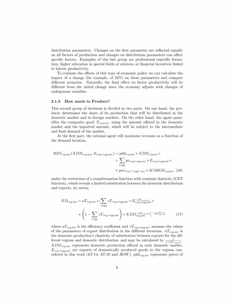
2.1.3 How much to Produce?

This second group of decisions is divided in two parts. On one hand, the pro-ducer determines the share of its production that will be distributed in thedomestic market and in foreign markets. On the other hand, the agent quan-ti�es the composite good Xreg;sec, using the amount o¤ered in the domesticmarket and the imported amount, which will be subject to the intermediateand �nal demand of the market.At the �rst part, the rational agent will maximise revenues as a function of

the demand location,

REVreg;sec(XDDreg;sec; Ereg;regg;sec) = pddreg;sec �XDDreg;sec+

+Xregg

pereg;regg;sec � Ereg;regg;sec+

+ pwereg;"regg";sec �MARGEreg;sec (16)

under the restriction of a transformation function with constant elasticity (CETfunction), which reveals a limited substitution between the domestic distributionand exports, by sector,

XDreg;sec = aTreg;sec � [Xregg

Treg;regg;sec � E��Treg;secreg;regg;sec+

+

1�

Xregg

Treg;regg;sec

!�XDD��Treg;sec

reg;sec ]� 1�Treg;sec (17)

where aTreg;sec is the e¢ ciency coe¢ cient and Treg;regg;sec assumes the valuesof the parameters of export distribution in the di¤erent locations. �Treg;sec isthe domestic production�s elasticity of substitution between exports for the dif-ferent regions and domestic distribution, and may be calculated by 1

1+�Treg;sec.

XDDreg;sec represents domestic production o¤ered in each domestic market,Ereg;regg;sec are exports of domestically produced goods to the regions con-sidered in this work (EU14, EU10 and ROW ), pddreg;sec represents prices of

8

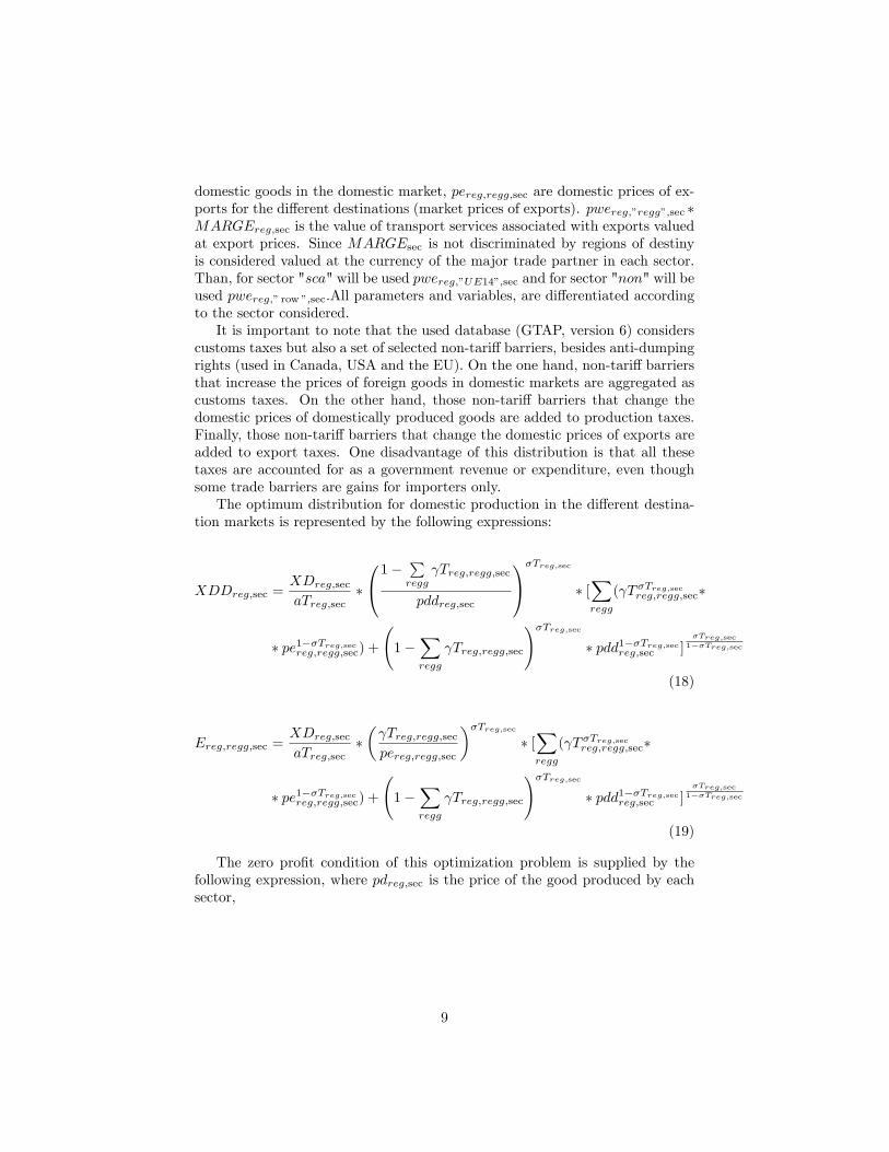
domestic goods in the domestic market, pereg;regg;sec are domestic prices of ex-ports for the di¤erent destinations (market prices of exports). pwereg;"regg";sec �MARGEreg;sec is the value of transport services associated with exports valuedat export prices. Since MARGEsec is not discriminated by regions of destinyis considered valued at the currency of the major trade partner in each sector.Than, for sector "sca" will be used pwereg;"UE14";sec and for sector "non" will beused pwereg;" row ";sec.All parameters and variables, are di¤erentiated accordingto the sector considered.It is important to note that the used database (GTAP, version 6) considers

customs taxes but also a set of selected non-tari¤ barriers, besides anti-dumpingrights (used in Canada, USA and the EU). On the one hand, non-tari¤ barriersthat increase the prices of foreign goods in domestic markets are aggregated ascustoms taxes. On the other hand, those non-tari¤ barriers that change thedomestic prices of domestically produced goods are added to production taxes.Finally, those non-tari¤ barriers that change the domestic prices of exports areadded to export taxes. One disadvantage of this distribution is that all thesetaxes are accounted for as a government revenue or expenditure, even thoughsome trade barriers are gains for importers only.The optimum distribution for domestic production in the di¤erent destina-

tion markets is represented by the following expressions:

XDDreg;sec =XDreg;secaTreg;sec

�

0@1�Pregg

Treg;regg;sec

pddreg;sec

1A�Treg;sec

� [Xregg

( T �Treg;secreg;regg;sec�

� pe1��Treg;secreg;regg;sec) +

1�

Xregg

Treg;regg;sec

!�Treg;sec� pdd1��Treg;secreg;sec ]

�Treg;sec1��Treg;sec

(18)

Ereg;regg;sec =XDreg;secaTreg;sec

�� Treg;regg;secpereg;regg;sec

��Treg;sec� [Xregg

( T �Treg;secreg;regg;sec�

� pe1��Treg;secreg;regg;sec) +

1�

Xregg

Treg;regg;sec

!�Treg;sec� pdd1��Treg;secreg;sec ]


(19)

The zero pro�t condition of this optimization problem is supplied by thefollowing expression, where pdreg;sec is the price of the good produced by eachsector,

9

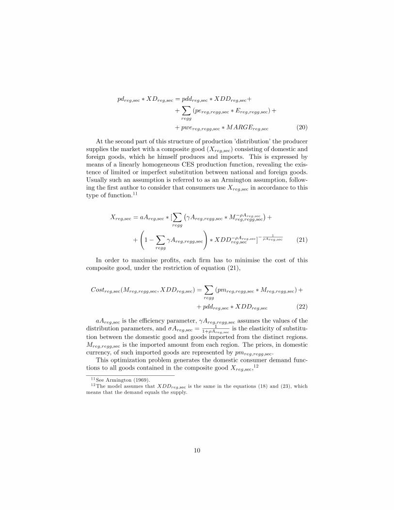
pdreg;sec �XDreg;sec = pddreg;sec �XDDreg;sec+

+Xregg

(pereg;regg;sec � Ereg;regg;sec)+

+ pwereg;regg;sec �MARGEreg;sec (20)

At the second part of this structure of production �distribution�the producersupplies the market with a composite good (Xreg;sec) consisting of domestic andforeign goods, which he himself produces and imports. This is expressed bymeans of a linearly homogeneous CES production function, revealing the exis-tence of limited or imperfect substitution between national and foreign goods.Usually such an assumption is referred to as an Armington assumption, follow-ing the �rst author to consider that consumers use Xreg;sec in accordance to thistype of function.11

Xreg;sec = aAreg;sec � [Xregg

� Areg;regg;sec �M��Areg;sec

reg;regg;sec

�+

+

1�

Xregg

Areg;regg;sec

!�XDD��Areg;sec

reg;sec ]� 1�Areg;sec (21)

In order to maximise pro�ts, each �rm has to minimise the cost of thiscomposite good, under the restriction of equation (21),

Costreg;sec(Mreg;regg;sec; XDDreg;sec) =Xregg

(pmreg;regg;sec �Mreg;regg;sec)+

+ pddreg;sec �XDDreg;sec (22)

aAreg;sec is the e¢ ciency parameter, Areg;regg;sec assumes the values of thedistribution parameters, and �Areg;sec = 1

1+�Areg;secis the elasticity of substitu-

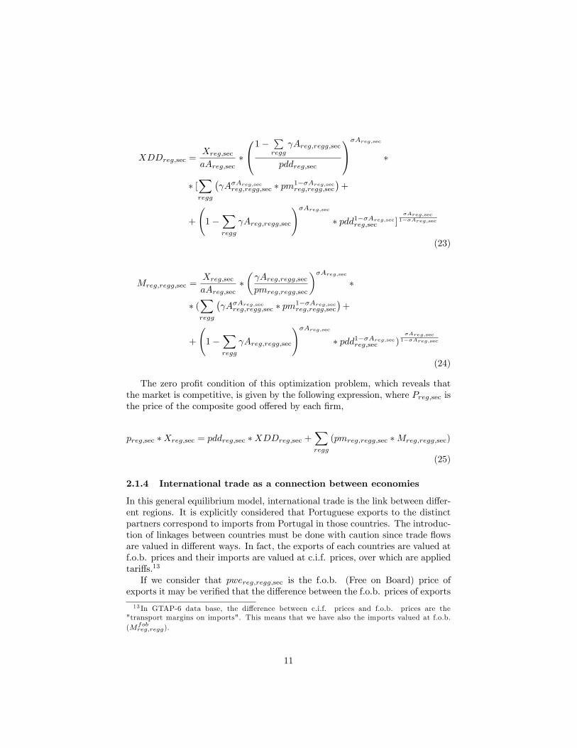
tion between the domestic good and goods imported from the distinct regions.Mreg;regg;sec is the imported amount from each region. The prices, in domesticcurrency, of such imported goods are represented by pmreg;regg;sec.This optimization problem generates the domestic consumer demand func-

tions to all goods contained in the composite good Xreg;sec,12

11See Armington (1969).12The model assumes that XDDreg;sec is the same in the equations (18) and (23), which

means that the demand equals the supply.

10

XDDreg;sec =Xreg;secaAreg;sec

�

0@1�Pregg

Areg;regg;sec

pddreg;sec

1A�Areg;sec

�

� [Xregg

� A�Areg;sec

reg;regg;sec � pm1��Areg;secreg;regg;sec

�+

+

1�

Xregg

Areg;regg;sec

!�Areg;sec

� pdd1��Areg;secreg;sec ]

�Areg;sec1��Areg;sec

(23)

Mreg;regg;sec =Xreg;secaAreg;sec

�� Areg;regg;secpmreg;regg;sec

��Areg;sec

�

� (Xregg

� A�Areg;sec

reg;regg;sec � pm1��Areg;secreg;regg;sec

�+

+

1�

Xregg

Areg;regg;sec

!�Areg;sec

� pdd1��Areg;secreg;sec )


(24)

The zero pro�t condition of this optimization problem, which reveals thatthe market is competitive, is given by the following expression, where Preg;sec isthe price of the composite good o¤ered by each �rm,

preg;sec �Xreg;sec = pddreg;sec �XDDreg;sec +Xregg

(pmreg;regg;sec �Mreg;regg;sec)

(25)

2.1.4 International trade as a connection between economies

In this general equilibrium model, international trade is the link between di¤er-ent regions. It is explicitly considered that Portuguese exports to the distinctpartners correspond to imports from Portugal in those countries. The introduc-tion of linkages between countries must be done with caution since trade �owsare valued in di¤erent ways. In fact, the exports of each countries are valued atf.o.b. prices and their imports are valued at c.i.f. prices, over which are appliedtari¤s.13

If we consider that pwereg;regg;sec is the f.o.b. (Free on Board) price ofexports it may be veri�ed that the di¤erence between the f.o.b. prices of exports

13 In GTAP-6 data base, the di¤erence between c.i.f. prices and f.o.b. prices are the"transport margins on imports". This means that we have also the imports valued at f.o.b.(Mfob

reg;regg).

11

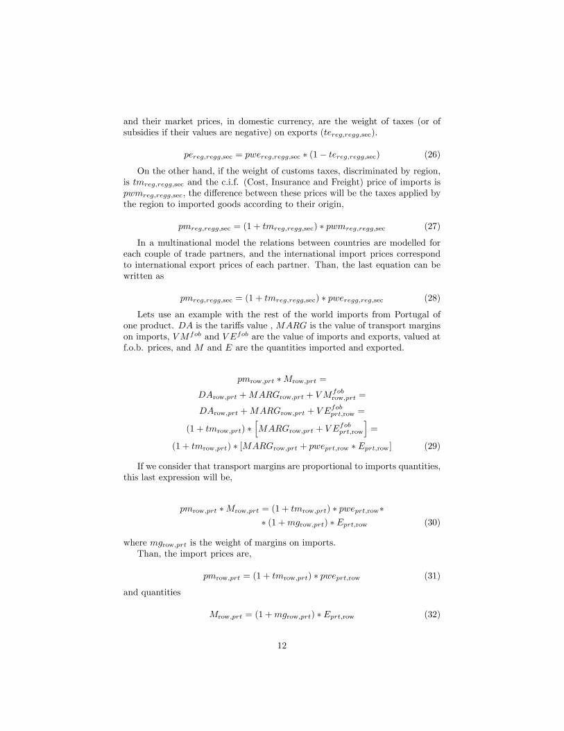
and their market prices, in domestic currency, are the weight of taxes (or ofsubsidies if their values are negative) on exports (tereg;regg;sec).

pereg;regg;sec = pwereg;regg;sec � (1� tereg;regg;sec) (26)

On the other hand, if the weight of customs taxes, discriminated by region,is tmreg;regg;sec and the c.i.f. (Cost, Insurance and Freight) price of imports ispwmreg;regg;sec, the di¤erence between these prices will be the taxes applied bythe region to imported goods according to their origin,

pmreg;regg;sec = (1 + tmreg;regg;sec) � pwmreg;regg;sec (27)

In a multinational model the relations between countries are modelled foreach couple of trade partners, and the international import prices correspondto international export prices of each partner. Than, the last equation can bewritten as

pmreg;regg;sec = (1 + tmreg;regg;sec) � pweregg;reg;sec (28)

Lets use an example with the rest of the world imports from Portugal ofone product. DA is the tari¤s value , MARG is the value of transport marginson imports, VMfob and V Efob are the value of imports and exports, valued atf.o.b. prices, and M and E are the quantities imported and exported.

pmrow;prt �Mrow;prt =

DArow;prt +MARGrow;prt + VMfobrow;prt =

DArow;prt +MARGrow;prt + V Efobprt;row =

(1 + tmrow;prt) �hMARGrow;prt + V E

fobprt;row

i=

(1 + tmrow;prt) � [MARGrow;prt + pweprt;row � Eprt;row] (29)

If we consider that transport margins are proportional to imports quantities,this last expression will be,

pmrow;prt �Mrow;prt = (1 + tmrow;prt) � pweprt;row�� (1 +mgrow;prt) � Eprt;row (30)

where mgrow;prt is the weight of margins on imports.Than, the import prices are,

pmrow;prt = (1 + tmrow;prt) � pweprt;row (31)

and quantities

Mrow;prt = (1 +mgrow;prt) � Eprt;row (32)

12

In the equation (30) it is possible to see the in�uence of each country oneach partner.In the context of this model, the Balance of Payments is represented by the

liquid �ow of goods and services.14

nXsec

(pweregg;reg;sec �Mreg;regg;sec) =nXsec

(pwereg;regg;sec � Ereg;regg;sec)+

+ SFreg;regg (33)

being SFreg;regg the foreign savings, i.e. the surplus of the Portuguese economyif negative, or de�cit if positive.

2.2 The Behaviour of the representative family

In this study a representative family is used as a proxy for all consumers. It isan assumption that erases social diversity, a characteristic of all economies, butis justi�ed by the fact that the objective of the model is the measurement ofthe e¤ects of economic policies in countries�external competitiveness and notat the level of income distribution among consumers.It is considered that the representative family is the owner of all production

factors and that the capital and labour endowments are exogenous, i.e. it isassumed that there is an external immobility of such factors. Unemployment isallowed in the model.The representative family maximises a non-homogeneous Stone-Gary utility

function, which produces a linear system of expenses (known as LES function),subject to a budget constraint.Family income is obtained with the selling of productive resources to �rms

(capital, skilled and unskilled labour), with the payment of unemployment sub-sidies and of other government transfers,

Y Hreg = pkreg � (1� dreg) �KSreg + plqreg � (LQSreg � UNEMPQreg)++ plureg � (LUSreg � UNEMPUreg) + TRFreg (34)

Y Hreg represents the family total income, KSreg, LUSreg and LQSreg arecapital and labour endowments, UNEMPQreg and UNEMPUreg are the un-employment of skilled and unskilled labour,15 TRFreg is the total amount offamily�s government transfers, and dreg is the rate of depreciation of capital.

14Capital �ows are not included in the equation because it is assumed that all factorsare immobile between countries. It is also not considered the transfers form Brussels, likestructural funds and other European funds. These issues are left for future developments ofthe model15 It is possible to use endogenous unemployment by means of a "Phillips� curve". This

curve relates the rate of change of the wage rate and the rate of change of the unemploymentrate. During this stage of the investigation, the unemployment is exogenous.

13

Families� expenses are allocated to income taxes (tyreg), savings (SHreg)and goods and services consumption (Creg;sec).Savings are a �xed share of the income, which means that the marginal

propensity to save (mpsreg) is constant, after deducting taxes paid to the gov-ernment,

SHreg = mpsreg � [Y Hreg � tyreg � (Y Hreg � TRFreg)] (35)

and allow the calculation of the income available to consumption (CBUDreg),

CBUDreg = Y Hreg � tyreg � (Y Hreg � TRFreg)� SHreg (36)

The consumer optimum choice is determined through the maximisation ofhis LES utility function (UHreg(Creg;sec)), subject to the budgetary constraintthat relates the income available to consumption with the value of expenses,

UHreg(Creg;sec) =Ysec

(Creg;sec � �Hreg;sec)�Hreg;sec (37)

whereXsec

�Hreg;sec = 1 and Creg;sec > �Hreg;sec � 0

s.t. CBUDreg =Xsec

[(1 + tcreg;sec) � preg;sec � Creg;sec] (38)

where �Hreg;sec represents the minimum amount of family consumption for eachgood, and preg;sec is the price of the goods sold in the domestic market (domesticand imported goods).16 The �nal private demand for goods and services isrepresented by,

Creg;sec = �Hreg;sec + �Hreg;sec � [(1 + tcreg;sec) � preg;sec]�1�

�(CBUDreg �

Xsecc

[(1 + tcreg;secc) � preg;secc � �Hreg;secc])

(39)

i.e.,

(1 + tcreg;sec) � preg;sec � Creg;sec = (1 + tcreg;sec) � preg;sec � �Hreg;sec+

+�Hreg;sec �(CBUDreg �

Xsecc

[(1 + tcreg;secc) � preg;secc � �Hreg;secc])

(40)

16When �Hreg;sec = 0; 8 sec, the LES function is transformed into a Cobb-Douglas function,which is homogenous of degree 1 (linear homogenous) if

Psec �Hsec = 1. Therefore, LES

functions are a generalization of Cobb-Douglas functions, and let the elasticity of substitutionto be di¤erent from 1. So, these functions may be more reasonable to study the consumerbehaviour.

14

It is interesting to note that (1 + tcreg;sec) � preg;sec � �Hreg;sec is the familyexpense that allows the attainment of the minimum level of consumption explicitin the utility function. �Hreg;sec[CBUDreg �

Psec(1 + tcreg;sec) � preg;sec �

�Hreg;sec] is the part of the available income that remains, after assuring theminimum level of consumption (residual income), and is expended in goods andin services in �xed parts for each sector, according to the parameters �Hreg;sec.

2.3 Government Behaviour

In what concerns the behaviour of the economic agent �government�, it is con-sidered that it is responsible for tax collection and transfers�payments to fam-ilies, namely unemployment subsidies and other transfers (such as pensionsor health related transfers). The considered taxes are those on consumption(tcreg;sec, tcgreg;sec, tcireg;sec, tcfreg;sec), on the use of capital (tkreg;sec) andlabour (tlqreg;sec and tlureg;sec), on income (tyreg), on imports (tmreg;regg;sec)and on exports (tereg;regg;sec), and on production (txdreg;sec). All these taxesare in proportion to the taxable basis.It is assumed that the government maximises a Cobb-Douglas utility function

(UGreg(CGreg;sec)) subject to an initially balanced budget. It is possible toassume a value for the budget de�cit or to bound it (e.g. 3% of GDP) bythe endogeneization of taxes. This option introduces a great complexity in themodel that should be avoided if the European economies are not really boundedby that assumption of Stability and Growth Plan.Total government revenues consist of total tax revenues (TAXRreg) since

the productive activities of the government are included in the activity of �rms.This is due to the fact that government behaviour in what concerns productiondecisions should be similar to that of private agents and also because the numberof totally public �rms are decreasing in number.

TAXRreg = tyreg � (Y Hreg � TRFreg) +Xsec

[preg;sec � (tcreg;sec � Creg;sec+

+ tcgreg;sec � CGreg;sec + tcireg;sec � Ireg sec) +Xsecc

(tcfreg;secc;sec�

� ioreg;secc;sec � preg;secc �XDreg;sec) + tkreg;sec � pkreg �Kreg;sec+

+ tlqreg;sec � plqreg � LQreg;sec + tlureg;sec � plureg � LUreg;sec+

+Xregg

(tmreg;regg;sec � pweregg;reg;sec �Mreg;regg;sec + tereg;regg;sec�

� pwereg;regg;sec � Ereg;regg;sec) + txdreg;sec � pdreg;sec �XDreg;sec](41)

Government pays unemployment subsidies at a rate trepreg as a share ofthe average wage and other transfers, such as pensions and health subsidies,that are constant in real terms and transformed into nominal variables using aLaspeyres price index (pcindexreg),

15

pcindexreg =Xsec

(1 + tctreg;sec) � ptreg;sec � C0reg;sec(1 + tc0reg;sec) � p0reg;sec � C0reg;sec

!(42)

where t is the moment in time (0 for values before the scenario simulation and1 for values after the scenario simulation).Total transfers (TRFreg) are expressed by the equation,

TRFreg = trepreg � (plqreg � UNEMPQreg + plureg � UNEMPUreg)++ TROreg � pcindexreg (43)

It is expected that government consumption decisions are also a result of themaximisation of a linearly homogeneous Cobb-Douglas utility function, subjectto the budget constraint, where �CGreg;sec is the income elasticity of the gov-ernment demand of goods and services and CGreg;sec the referred demand,

UGreg(CGreg;sec) =nQsecCG�CGreg;sec

reg;sec beingnXsec

�CGreg;sec = 1 (44)

s.t.

TAXRreg�TRFreg�pcindexreg�SGreg =nXsec

(1 + tcgreg;sec)�preg;sec�CGreg;sec

(45)where pcindexreg�SGreg is the budget balance, being SGreg the real governmentsaving and tcgreg;sec is the tax weight on public consumption.Government�s demand for goods and services, obtained via the optimization,

as the following expression,

(1 + tcgreg;sec) � preg;sec � CGreg;sec = �CGreg;sec��(TAXRreg � TRFreg � pcindexreg � SGreg) (46)

As it would be expected, government�s nominal expenditure in each goodand service is a �xed share of its revenues. If the demand functions are added,across sectors, the result is the government�s budget constraint, which puts inevidence the existence of constant scale returns linked to the homogeneity ofthis agent�s utility function.

2.4 Investment Demand

The demand for investment will be included in the model in a very simple way,considering investment as investment goods, i.e. goods and services identicalto those demanded by �rms and consumers, valued at market prices (including

16

taxes). It is considered that there is an entity that allocates savings across in-vestment goods, in all sectors, in accordance to a Cobb-Douglas utility function(UIreg(Ireg;sec)), where Ireg;sec is the amount of investment goods and �Ireg;secis the income elasticity of the investment good demand.

UIreg(Ireg;sec) =nQsecI�Ireg;secreg;sec where

nXsec=1

�Ireg;sec = 1 (47)

The demand expression is determined by the maximisation of this utility func-tion, subject to the constraint of total savings (Sreg) where tcireg;sec is theweight of taxes on the consumption of the goods used as investment goods,

Sreg =nXsec

Ireg;sec � preg;sec � (1 + tcireg;sec) (48)

being total savings equal to the following identity,

Sreg = SHreg + pcindexreg � SGreg +Xregg

(SFreg;regg)+

+Xsec

dreg � pkreg �Kreg;sec �MARGEreg;sec � pwereg;regg;sec (49)

The solution of the maximisation problem is

(1 + tcireg;sec) � preg;sec � Ireg;sec = �Ireg;sec � Sreg (50)

i.e.,

Ireg;sec = �Ireg;sec � Sreg � [(1 + tcireg;sec) � preg;sec]�1 (51)

2.5 General equilibrium in the economy

The general equilibrium in the economy implies the equality between supplyand demand in all markets (goods and services, capital and labour). Than, inlabour market the demand must equal the supply of the two types of labour(LUS for the unskilled labour and LQS for the skilled), liquid of unemployment,X

sec

LQreg;sec = LQSreg � UNEMPQreg (52)

Xsec

LUreg;sec = LUSreg � UNEMPUreg (53)

The same should occur in the capital market, where it is considered thatthere are no unemployed resources,

17

Xsec

Kreg;sec = KSreg (54)

as well as in goods and services market,

Xreg;sec = Creg;sec + Ireg;sec +Xsecc

(ioreg;sec;secc �XDreg;secc) + CGreg;sec (55)

As in all general equilibrium models the Walras Law must be satis�ed. Thislaw say brie�y that in an economy with "m" markets, if "m� 1" markets are inequilibrium, than the last market will be necessarily in equilibrium. This impliesthat we must not consider one of the last four equations during the solvement.17

Finally, to close the model the numeraire will be the price of one of thefactors of production (pkreg, plqreg or plureg).The factor endowments in the economy are exogenous (KSreg, LQSreg and

LUSreg), as well as the unemployment levels (UNEMPQreg and UNEMPUreg),other government transfers for the households (TROreg), transport services re-lated to exports (MARGEreg;sec), government savings (SGreg) and foreign sav-ings between countries of the region "rest of the world" (SFreg;regg). This lastclosure equation exist since walras law is satis�ed.

2.6 Data base

In this version of the model is used the GTAP (version 6) data base for majorvariables, except for unemployment levels (UNEMPQreg and UNEMPUreg),rates of unemployment subsidy (trepreg), other government transfers for thehouseholds (TROreg), all transformation and substitution elasticities (�Freg;sec,�Treg;sec, �Areg;sec) and the minimum amount of families consumption for eachgood (�Hreg;sec). The 87 regions of the data base are aggregated into 4 regions(Portugal, EU14, EU10 and ROW). In respect to sectors, the 57 sectors ofthe data bade are aggregated into 6 already reported. The great advantage ofthis data base is the possibility of direct comparison of di¤erent input-outputmatrixes, and its easy accessibility. In what concerns to the parameters thatnot exist in this data bade, the statistical sources are di¤erent.For the unemployment level it will be used the rates of National Statistic

Institute (INE), for Portuguese levels and the rates of EUROSTAT for remainingregions.18

The parameter trepreg is calculated with EUROSTAT data, as the weightof unemployment subsidy per unemployed person, in each region, relatively tothe nominal compensation per employee.19

17 It will be ignored the equation of the market which price will be the numeraire.18See INE (2001) and http://epp.eurostat.ec.europa.eu/.19See "Out-of-work income maintenance and support" and "Nominal compensation per

employee" in http://epp.eurostat.ec.europa.eu/.

18

The source of other government transfers for the households (TROreg) isNational Accounts of INE, and EUROSTAT20 To avoid any incompatibility be-tween this statistics sources and GTAP data base, this parameter is introducedas a percentage of households consumption at current prices.The unknown parameter of the household utility function (�Hreg;sec) is very

subjective because it depends mainly on household preferences. Since we haveonly one representative household in each region, it is almost a random choice.The option made is the average consumption in the beginning of ninety decade,when started the accession negotiations to EU.21 So, is assumed that house-holds considers the consumption level before the start of European enlargementprocess as the minimum acceptable.With respect to substitution and transformation elasticities the sources are

di¤erent. For elasticities of substitution between production factors (�Freg;sec),the values generated by the general equilibrium program "RunGTAP - Version5" of GTAP data base are used, considering the same sectorial and regionalaggregation as in this model. For elasticities of substitution between domesticand imported goods (�Areg;sec), the values considered by OECD in a tari¤ tradesimulator (the most used in international literature) are used.(OCDE (2003))The discrimination between regions are made using the respective weights ofeach product in each sector.Finally, for transformation elasticities (�Treg;sec), an approximation are cal-

culated, using total �ows,in Portugal, and for the other regions are applied thevalues used in DART model.22

3 Alternative Scenarios and Results

The purpose of this paper is the identi�cation of which type of labour (skilledor unskilled) permits the greater improvement of Portuguese competitivenesswhen its productivity increase, and in which sector that happen. Naturally, toget the �nal decision we need to know the cost of each alternative of policy toincrease the labour productivity.Since each sector has a di¤erent weight on both intermediate and �nal con-

sumption (domestic and foreigner), the increase of labour productivity also has adi¤erent impact on the promotion of exports and imports. Thus, it is importantto test the e¤ect of changes in productivity of both skilled and unskilled labour,in di¤erent sectors and in di¤erent combinations. We will test a 10% change indistribution parameters related with labour ( Fqprt;sec and Fuprt;sec).The following scenarios will be tested:

20See "Quadro de Contas Económicas Integradas", INE (2004) andhttp://epp.eurostat.ec.europa.eu/.21Calculus are based on national statistics (INE and Portuguese Bank) and european sta-

tistics (http://epp.eurostat.ec.europa.eu/).22See

19

Table 3: Scenarios (increases of 10%)C1 - increase of Fq and Fu in all sectorsC2 - increase of Fq in all sectorsC3 - increase of Fu in all sectorsC4 - increase of Fq and Fu in sector "res"C5 - increase of Fq and Fu in sector "lab"C6 - increase of Fq and Fu in sector "spe"C7 - increase of Fq and Fu in sector "sca"C8 - increase of Fq and Fu in sector "rd"C9 - increase of Fq and Fu in sector "non"C10 - increase of Fq and Fu in sectors "lab", "spe", "sca" and "rd"C11 - increase of Fu in all sectors and of Fq in sectors "res" and

"lab"C12 - increase of Fu in all sectors and of Fq in sectors "res", "lab"

and "non"C13 - increase of Fu in all sectors and of Fq in sectors "res", "lab",

"non" and "sca"

Since it is being used a multi-national and multi-sector general equilibriummodel, it is possible to evaluate changes in all trade �ows of all regions. Theonly closure condition that is acting on the results is the fact that foreignersaving between countries in "rest of the world" region. Notwithstanding, it isnot supposed that changes in Portuguese labour productivity will, in fact, makeany di¤erence in these region. So, it is not a refraining condition.The e¤ects can be seen in terms of relative changes of all variables. However,

in this paper will be only presented the results for exports, agents utility andequivalent variation index.It is important to notice that di¤erent size of the regions and the sectors

implies a careful analyses.We can see that trade relations between Portugal and EU10 are insigni�cant

both in exports and in imports (see tables 4 and 5). This insigni�cance is alsovalid for sector "rd" ("research and development").

Table 4: Weight of each sector exports ontotal exports, by partner (%)

res lab spe sca rd non TotalyPRT!UE14 13,81 26,21 18,22 28,07 0,80 12,90 21,884827PRT!UE10 6,50 14,46 35,10 24,36 1,06 18,52 0,5335088PRT!ROW 14,17 15,33 13,36 20,74 2,33 34,07 9,2026437

y- monetary units.

Table 5: Weight of each sector imports ontotal imports, by partner (%)

20

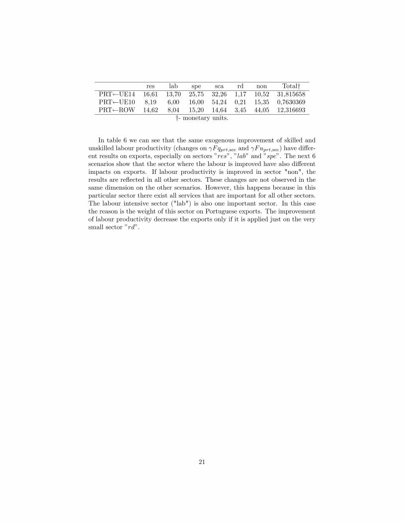
res lab spe sca rd non TotalyPRT UE14 16,61 13,70 25,75 32,26 1,17 10,52 31,815658PRT UE10 8,19 6,00 16,00 54,24 0,21 15,35 0,7630369PRT ROW 14,62 8,04 15,20 14,64 3,45 44,05 12,316693

y- monetary units.

In table 6 we can see that the same exogenous improvement of skilled andunskilled labour productivity (changes on Fqprt;sec and Fuprt;sec) have di¤er-ent results on exports, especially on sectors "res", "lab" and "spe". The next 6scenarios show that the sector where the labour is improved have also di¤erentimpacts on exports. If labour productivity is improved in sector "non", theresults are re�ected in all other sectors. These changes are not observed in thesame dimension on the other scenarios. However, this happens because in thisparticular sector there exist all services that are important for all other sectors.The labour intensive sector ("lab") is also one important sector. In this casethe reason is the weight of this sector on Portuguese exports. The improvementof labour productivity decrease the exports only if it is applied just on the verysmall sector "rd".

21

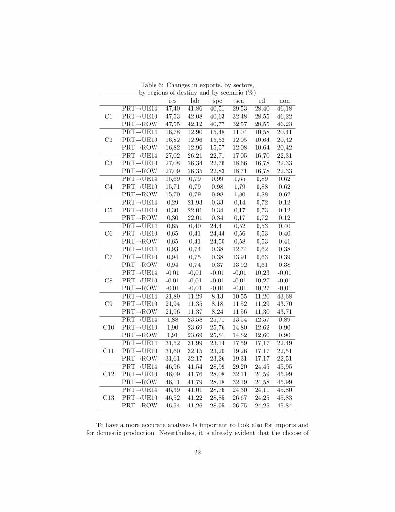
Table 6: Changes in exports, by sectors,by regions of destiny and by scenario (%)

res lab spe sca rd nonPRT!UE14 47,40 41,86 40,51 29,53 28,40 46,18

C1 PRT!UE10 47,53 42,08 40,63 32,48 28,55 46,22PRT!ROW 47,55 42,12 40,77 32,57 28,55 46,23PRT!UE14 16,78 12,90 15,48 11,04 10,58 20,41






C7 PRT!UE10 0,94 0,75 0,38 13,91 0,63 0,39PRT!ROW 0,94 0,74 0,37 13,92 0,61 0,38PRT!UE14 -0,01 -0,01 -0,01 -0,01 10,23 -0,01

C8 PRT!UE10 -0,01 -0,01 -0,01 -0,01 10,27 -0,01PRT!ROW -0,01 -0,01 -0,01 -0,01 10,27 -0,01PRT!UE14 21,89 11,29 8,13 10,55 11,20 43,68





C13 PRT!UE10 46,52 41,22 28,85 26,67 24,25 45,83PRT!ROW 46,54 41,26 28,95 26,75 24,25 45,84

To have a more accurate analyses is important to look also for imports andfor domestic production. Nevertheless, it is already evident that the choose of

22

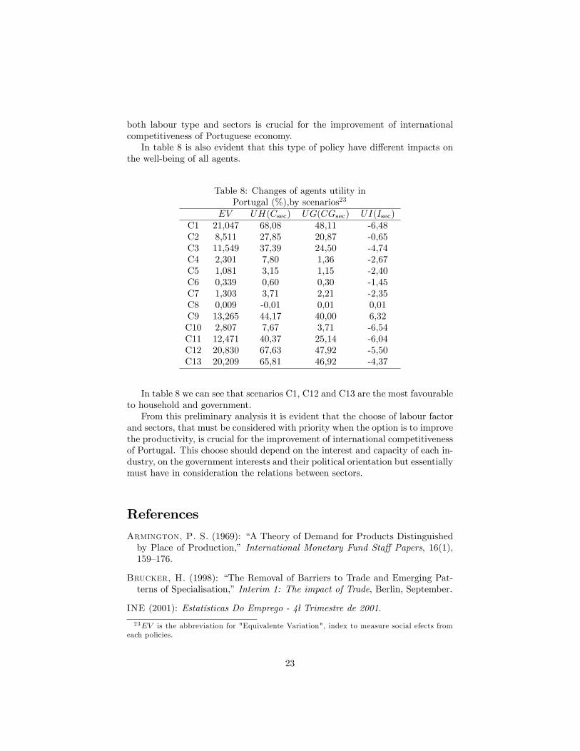
both labour type and sectors is crucial for the improvement of internationalcompetitiveness of Portuguese economy.In table 8 is also evident that this type of policy have di¤erent impacts on

the well-being of all agents.

Table 8: Changes of agents utility inPortugal (%),by scenarios23

EV UH(Csec) UG(CGsec) UI(Isec)C1 21,047 68,08 48,11 -6,48C2 8,511 27,85 20,87 -0,65C3 11,549 37,39 24,50 -4,74C4 2,301 7,80 1,36 -2,67C5 1,081 3,15 1,15 -2,40C6 0,339 0,60 0,30 -1,45C7 1,303 3,71 2,21 -2,35C8 0,009 -0,01 0,01 0,01C9 13,265 44,17 40,00 6,32C10 2,807 7,67 3,71 -6,54C11 12,471 40,37 25,14 -6,04C12 20,830 67,63 47,92 -5,50C13 20,209 65,81 46,92 -4,37

In table 8 we can see that scenarios C1, C12 and C13 are the most favourableto household and government.From this preliminary analysis it is evident that the choose of labour factor

and sectors, that must be considered with priority when the option is to improvethe productivity, is crucial for the improvement of international competitivenessof Portugal. This choose should depend on the interest and capacity of each in-dustry, on the government interests and their political orientation but essentiallymust have in consideration the relations between sectors.

References

Armington, P. S. (1969): �A Theory of Demand for Products Distinguishedby Place of Production,� International Monetary Fund Sta¤ Papers, 16(1),159�176.

Brucker, H. (1998): �The Removal of Barriers to Trade and Emerging Pat-terns of Specialisation,�Interim 1: The impact of Trade, Berlin, September.

INE (2001): Estatísticas Do Emprego - 4÷Trimestre de 2001.

23EV is the abbreviation for "Equivalente Variation", index to measure social efects fromeach policies.

23

(2004): Contas Nacionais Anuais (Base 2000) 1995-2003.

OCDE (2003): �Tari¤s and Trade: OECD Query and Simulation Package,�(CD-ROM).

Silberberg, E., and W. C. Suen (2001): The Structure of Economics: AMathematical Analysis. McGraw-Hill Publishing Company.

24

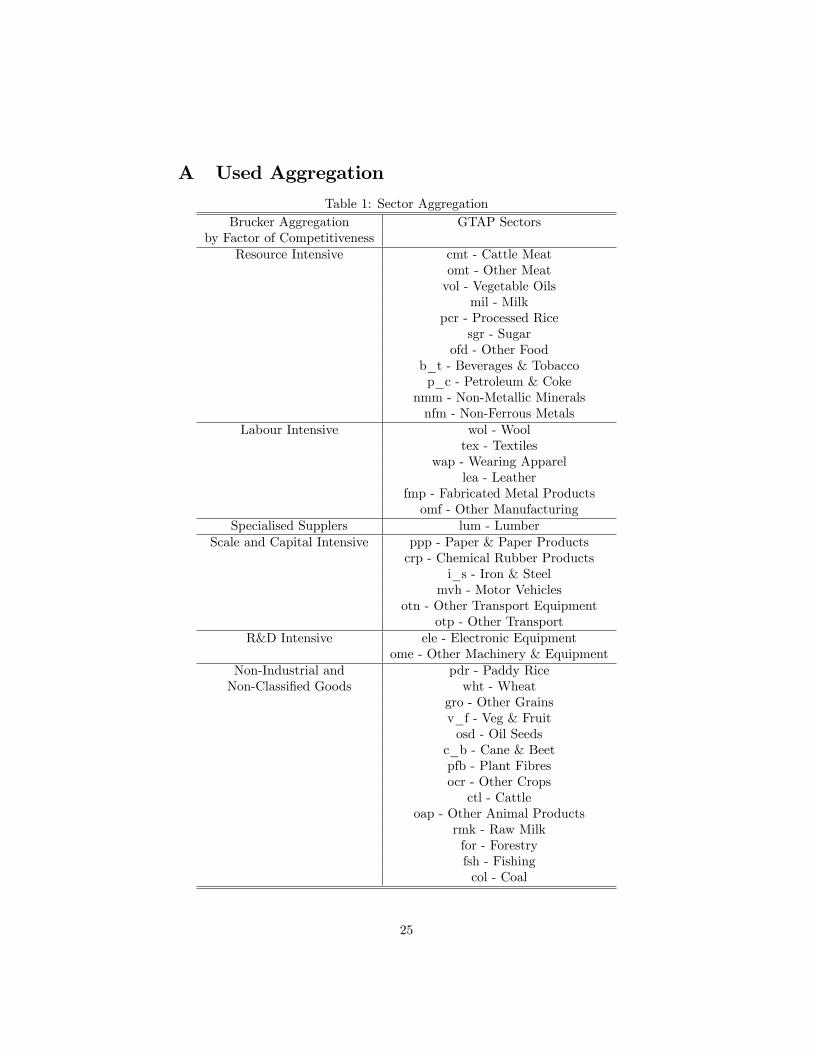
A Used Aggregation

Table 1: Sector AggregationBrucker Aggregation GTAP Sectors

by Factor of CompetitivenessResource Intensive cmt - Cattle Meat

omt - Other Meatvol - Vegetable Oils

mil - Milkpcr - Processed Rice

sgr - Sugarofd - Other Food

b_t - Beverages & Tobaccop_c - Petroleum & Coke

nmm - Non-Metallic Mineralsnfm - Non-Ferrous Metals

Labour Intensive wol - Wooltex - Textiles

wap - Wearing Apparellea - Leather

fmp - Fabricated Metal Productsomf - Other Manufacturing

Specialised Supplers lum - LumberScale and Capital Intensive ppp - Paper & Paper Products

crp - Chemical Rubber Productsi_s - Iron & Steel

mvh - Motor Vehiclesotn - Other Transport Equipment

otp - Other TransportR&D Intensive ele - Electronic Equipment

ome - Other Machinery & EquipmentNon-Industrial and pdr - Paddy RiceNon-Classi�ed Goods wht - Wheat

gro - Other Grainsv_f - Veg & Fruitosd - Oil Seeds

c_b - Cane & Beetpfb - Plant Fibresocr - Other Cropsctl - Cattle

oap - Other Animal Productsrmk - Raw Milkfor - Forestryfsh - Fishingcol - Coal

25

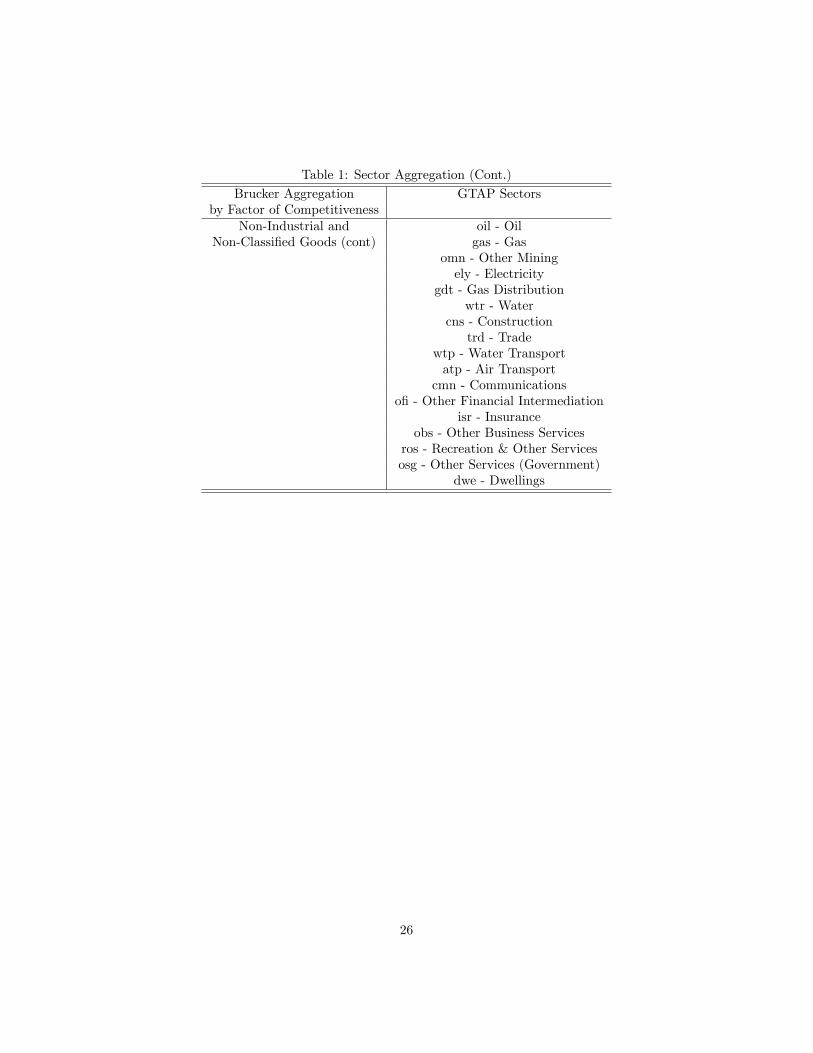
Table 1: Sector Aggregation (Cont.)Brucker Aggregation GTAP Sectors

by Factor of CompetitivenessNon-Industrial and oil - Oil

Non-Classi�ed Goods (cont) gas - Gasomn - Other Miningely - Electricity

gdt - Gas Distributionwtr - Water

cns - Constructiontrd - Trade

wtp - Water Transportatp - Air Transport

cmn - Communicationso� - Other Financial Intermediation

isr - Insuranceobs - Other Business Services

ros - Recreation & Other Servicesosg - Other Services (Government)

dwe - Dwellings

26

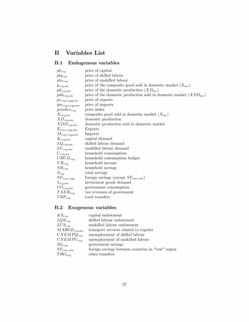
B Variables List

B.1 Endogenous variables

pkreg price of capitalplqreg price of skilled labourplureg price of unskilled labourpreg;sec price of the composite good sold in domestic market (Xsec)pdreg;sec price of the domestic production (XDsec)pddreg;sec price of the domestic production sold in domestic market (XDDsec)pereg;regg;sec price of exportspmreg;regg;sec price of importspcindexreg price indexXreg;sec composite good sold in domestic market (Xsec)XDreg;sec domestic productionXDDreg;sec domestic production sold in domestic marketEreg;regg;sec ExportsMreg;regg;sec ImportsKreg;sec capital demandLQreg;sec skilled labour demandLUreg;sec unskilled labour demandCreg;sec household consumptionCBUDreg household consumption budgetY Hreg household incomeSHreg household savingsSreg total savingsSFreg;regg foreign savings (except SFrow;row)Ireg;sec investment goods demandCGreg;sec government consumptionTAXRreg tax revenues of governmentTRFreg total transfers

B.2 Exogenous variables

KSreg capital endowmentLQSreg skilled labour endowmentLUSreg unskilled labour endowmentMARGEreg;sec transport services related to exportsUNEMPQreg unemployment of skilled labourUNEMPUreg unemployment of unskilled labourSGreg government savingsSFrow;row foreign savings between countries in "row" regionTROreg other transfers

27

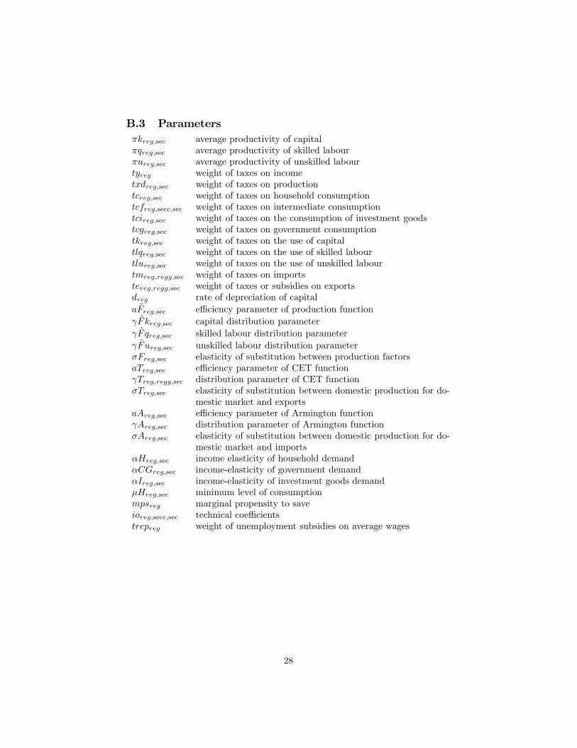
B.3 Parameters�kreg;sec average productivity of capital�qreg;sec average productivity of skilled labour�ureg;sec average productivity of unskilled labourtyreg weight of taxes on incometxdreg;sec weight of taxes on productiontcreg;sec weight of taxes on household consumptiontcfreg;secc;sec weight of taxes on intermediate consumptiontcireg;sec weight of taxes on the consumption of investment goodstcgreg;sec weight of taxes on government consumptiontkreg;sec weight of taxes on the use of capitaltlqreg;sec weight of taxes on the use of skilled labourtlureg;sec weight of taxes on the use of unskilled labourtmreg;regg;sec weight of taxes on importstereg;regg;sec weight of taxes or subsidies on exportsdreg rate of depreciation of capitala ~Freg;sec e¢ ciency parameter of production function ~Fkreg;sec capital distribution parameter ~Fqreg;sec skilled labour distribution parameter ~Fureg;sec unskilled labour distribution parameter�Freg;sec elasticity of substitution between production factorsaTreg;sec e¢ ciency parameter of CET function Treg;regg;sec distribution parameter of CET function�Treg;sec elasticity of substitution between domestic production for do-

mestic market and exportsaAreg;sec e¢ ciency parameter of Armington function Areg;sec distribution parameter of Armington function�Areg;sec elasticity of substitution between domestic production for do-

mestic market and imports�Hreg;sec income elasticity of household demand�CGreg;sec income-elasticity of government demand�Ireg;sec income-elasticity of investment goods demand�Hreg;sec minimum level of consumptionmpsreg marginal propensity to saveioreg;secc;sec technical coe¢ cientstrepreg weight of unemployment subsidies on average wages

28

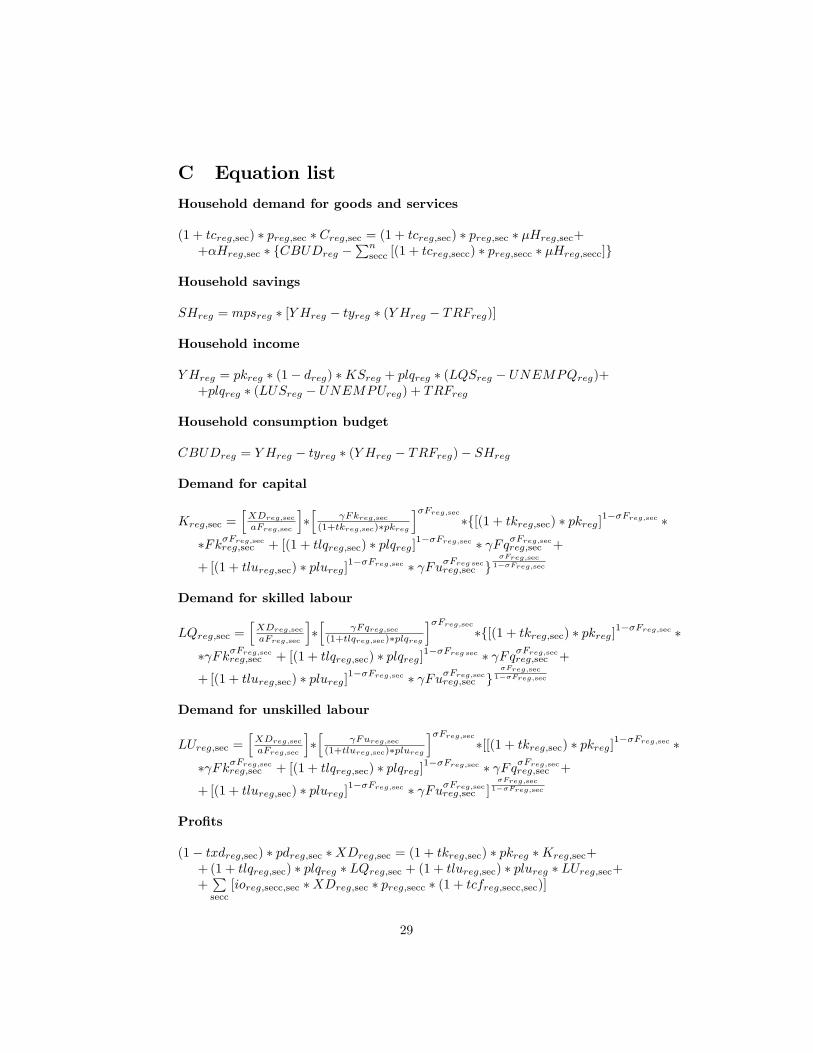
C Equation list

Household demand for goods and services

(1 + tcreg;sec) � preg;sec � Creg;sec = (1 + tcreg;sec) � preg;sec � �Hreg;sec++�Hreg;sec � fCBUDreg �

Pnsecc [(1 + tcreg;secc) � preg;secc � �Hreg;secc]g

Household savings

SHreg = mpsreg � [Y Hreg � tyreg � (Y Hreg � TRFreg)]

Household income

Y Hreg = pkreg � (1� dreg) �KSreg + plqreg � (LQSreg � UNEMPQreg)++plqreg � (LUSreg � UNEMPUreg) + TRFreg

Household consumption budget

CBUDreg = Y Hreg � tyreg � (Y Hreg � TRFreg)� SHreg

Demand for capital

Kreg;sec =hXDreg;sec

aFreg;sec

i�h

Fkreg;sec(1+tkreg;sec)�pkreg

i�Freg;sec�f[(1 + tkreg;sec) � pkreg]1��Freg;sec �

�Fk�Freg;secreg;sec + [(1 + tlqreg;sec) � plqreg]1��Freg;sec � Fq�Freg;secreg;sec +

+ [(1 + tlureg;sec) � plureg]1��Freg;sec � Fu�Freg secreg;sec g�Freg;sec

1��Freg;sec

Demand for skilled labour

LQreg;sec =hXDreg;sec

aFreg;sec

i�h

Fqreg;sec(1+tlqreg;sec)�plqreg

i�Freg;sec�f[(1 + tkreg;sec) � pkreg]1��Freg;sec �

� Fk�Freg;secreg;sec + [(1 + tlqreg;sec) � plqreg]1��Freg sec � Fq�Freg;secreg;sec +

+ [(1 + tlureg;sec) � plureg]1��Freg;sec � Fu�Freg;secreg;sec g�Freg;sec

1��Freg;sec

Demand for unskilled labour

LUreg;sec =hXDreg;sec

aFreg;sec

i�h

Fureg;sec(1+tlureg;sec)�plureg

i�Freg;sec�[[(1 + tkreg;sec) � pkreg]1��Freg;sec �

� Fk�Freg;secreg;sec + [(1 + tlqreg;sec) � plqreg]1��Freg;sec � Fq�Freg;secreg;sec +


1��Freg;sec

Pro�ts

(1� txdreg;sec) � pdreg;sec �XDreg;sec = (1 + tkreg;sec) � pkreg �Kreg;sec++(1 + tlqreg;sec) � plqreg � LQreg;sec + (1 + tlureg;sec) � plureg � LUreg;sec++Psecc

[ioreg;secc;sec �XDreg;sec � preg;secc � (1 + tcfreg;secc;sec)]

29

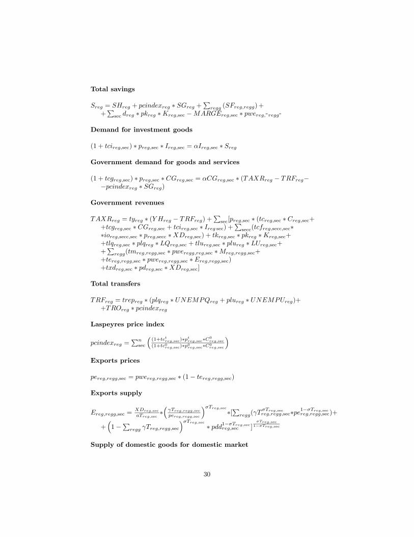
Total savings

Sreg = SHreg + pcindexreg � SGreg +P

regg (SFreg;regg)++P

sec dreg � pkreg �Kreg;sec �MARGEreg;sec � pwereg;"regg"

Demand for investment goods

(1 + tcireg;sec) � preg;sec � Ireg;sec = �Ireg;sec � Sreg

Government demand for goods and services

(1 + tcgreg;sec) � preg;sec � CGreg;sec = �CGreg;sec � (TAXRreg � TRFreg��pcindexreg � SGreg)

Government revenues

TAXRreg = tyreg � (Y Hreg � TRFreg) +P

sec[preg;sec � (tcreg;sec � Creg;sec++tcgreg;sec � CGreg;sec + tcireg;sec � Ireg sec) +

Psecc(tcfreg;secc;sec�

�ioreg;secc;sec � preg;secc �XDreg;sec) + tkreg;sec � pkreg �Kreg;sec++tlqreg;sec � plqreg � LQreg;sec + tlureg;sec � plureg � LUreg;sec++P

regg(tmreg;regg;sec � pweregg;reg;sec �Mreg;regg;sec++tereg;regg;sec � pwereg;regg;sec � Ereg;regg;sec)+txdreg;sec � pdreg;sec �XDreg;sec]

Total transfers

TRFreg = trepreg � (plqreg � UNEMPQreg + plureg � UNEMPUreg)++TROreg � pcindexreg

Laspeyres price index

pcindexreg =Pn

sec

�(1+tctreg;sec)�p

treg;sec�C

0reg;sec

(1+tc0reg;sec)�p0reg;sec�C0reg;sec

�Exports prices

pereg;regg;sec = pwereg;regg;sec � (1� tereg;regg;sec)

Exports supply

Ereg;regg;sec =XDreg;sec

aTreg;sec�� Treg;regg;secpereg;regg;sec

��Treg;sec�[P

regg( T�Treg;secreg;regg;sec�pe1��Treg;secreg;regg;sec)+

+�1�

Pregg Treg;regg;sec

��Treg;sec� pdd1��Treg;secreg;sec ]


Supply of domestic goods for domestic market

30

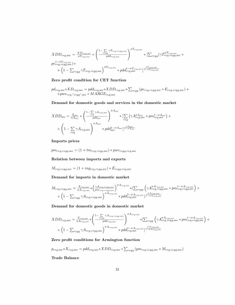
XDDreg;sec =XDreg;sec

aTreg;sec� 1�

Pregg

Treg;regg;sec

pddreg;sec

!�Treg;sec� [P

regg( T�Treg;secreg;regg;sec �

pe1��Treg;secreg;regg;sec)+

+�1�

Pregg Treg;regg;sec

��Treg;sec� pdd1��Treg;secreg;sec ]


Zero pro�t condition for CET function

pdreg;sec�XDreg;sec = pddreg;sec�XDDreg;sec+P

regg (pereg;regg;sec � Ereg;regg;sec)++pwereg;"regg";sec �MARGEreg;sec

Demand for domestic goods and services in the domestic market

XDDsec =Xsec

aAsec� 1�

Preg

Areg;sec

pddsec

!�Asec

� [Preg

� A�Asec

reg;sec � pm1��Asecreg;sec

�+

+

1�

Preg Areg;sec

!�Asec

� pdd1��Asecsec ]

�Asec1��Asec

Imports prices

pmreg;regg;sec = (1 + tmreg;regg;sec) � pweregg;reg;sec

Relation between imports and exports

Mreg;regg;sec = (1 +mgreg;regg;sec) � Eregg;reg;sec

Demand for imports in domestic market

Mreg;regg;sec =Xreg;sec

aAreg;sec�� Areg;regg;sec

pmreg;regg;sec

��Areg;sec

�(P

regg

� A

�Areg;secreg;regg;sec � pm1��Areg;sec

reg;regg;sec

�+

+�1�

Pregg Areg;regg;sec

��Areg;sec

� pdd1��Areg;secreg;sec )


Demand for domestic goods in domestic market

XDDreg;sec =Xreg;sec

aAreg;sec� 1�

Pregg

Areg;regg;sec

pddreg;sec

!�Areg;sec

�[P

regg

� A

�Areg;secreg;regg;sec � pm1��Areg;sec

reg;regg;sec

�+

+�1�

Pregg Areg;regg;sec

��Areg;sec

� pdd1��Areg;secreg;sec ]


Zero pro�t conditions for Armington function

preg;sec�Xreg;sec = pddreg;sec�XDDreg;sec+P

regg (pmreg;regg;sec �Mreg;regg;sec)

Trade Balance

31

Psec (pweregg;reg;sec �Mreg;regg;sec) =

Psec (pwereg;regg;sec � Ereg;regg;sec)+SFreg;regg

Equilibrium in skilled labour marketPsec LQreg;sec = LQSreg � UNEMPQreg

Equilibrium in unskilled labour marketPsec LUreg;sec = LUSreg � UNEMPUreg

Equilibrium in capital marketPsecKreg;sec = KSreg

Equilibrium in goods and services market

Xreg;sec = Creg;sec + Ireg;sec +P

secc(ioreg;sec;secc �XDreg;secc) + CGreg;sec

32

Documents

How to improve international competitiveness of Portuguese ... · How to improve international competitiveness of Portuguese economy ... 5See Silberberg and Suen (2001) for speci–c