How to measure lifetime for Robustness Validation step by step

How to measure lifetime for

Robustness Validation

– step by step

Electronic Components and Systems Division

How to measure lifetime for Robustness Validation 2

Impressum

How to measure lifetime for Robustness Validation -

step by step

Published by:

Robustness Validation Forum

ZVEI - German Electrical and Electronic Manufacturers ‘Association e.V.

Electronic Components and Systems (ECS) Division

Lyoner Straße 9

60528 Frankfurt am Main, Germany

Phone: +49 69 6302 402

Fax: +49 69 6302 407

E-mail: [email protected]

www.zvei.org/ecs

Contact person:

Dr.-Ing. Rolf Winter

Picture credits, title:

Fotolia 24076108_©ArchMen and

ZVEI - German Electrical and Electronic Manufacturers‘ Association e.V.

Measurement Data and Graphics: Robert BOSCH GmbH

November 2012 / Revision 1.9

This document may be reproduced free of charge in any format or medium providing it is

reproduced accurately and not used in a misleading context. The material must be acknowledged

as ZVEI copyright and the title of the document has to be specified. A complimentary copy of the

document where ZVEI material is quoted has to be provided. Every effort was made to ensure

that the information given herein is accurate, but no legal responsibility is accepted for any

errors, omissions or misleading statements in this information. The Document and supporting

materials can be found on the ZVEI website at:

www.zvei.org under the rubric "Publikationen" or directly under

www.zvei.org/RobustnessValidation

http://www.zvei.org/

http://www.zvei.org/RobustnessValidation


Content

1. Starting a lifetime evaluation 5

2. Pre Evaluation – doing principle investigations 7

3. Performing investigation on several devices 9

4. Generating a lifetime distribution 11

5. Defining the failure criterion 14

6. Evaluating the lifetime distribution parameters 16

7. Lifetime at different stress values 22

8. Applying the acceleration model 25

9. Calculating the lifetime in the field 28

10. Further Reading 31

11. Appendix A: Strange curves – what to do? 32

12. Appendix B: Measurement data 35


Preamble

The objective of this document is to introduce the concepts of life time testing, distribution,

acceleration and prediction to those who are not familiar with and/or are beginners in reliability

engineering and statistics. The reader will be guided step by step by making use of simple and

representative examples in which results of testing until failure are used. Therefore, in addition

the importance of failure criteria and understanding failure mechanisms will be discussed and

explained. Finally, in case the reader is interested in more details, a list of recommended

literature is given.

Foreword

The quality of electronic products we buy and the competitiveness of the electronics industry

depend on being able to make sound quality and reliability predictions. Qualification measures

must be useful and accurate data to provide added value. Increasingly, manufacturers of

semiconductor components must be able to show that they are producing meaningful results for

the reliability of their products under defined mission profiles from the whole supply chain.

Reliability is the probability that a semiconductor component will perform in accordance with

expectations for a predetermined period of time in a given environment. To be efficient reliability

testing has to compress this time scale by accelerated stresses to generate knowledge about the

time to failure. To meet any reliability objective, requires comprehensive knowledge of the

interaction of failure modes, failure mechanisms, the mission profile and the design of the

product.

In recent years the Robustness Validation Methodology is becoming more and more commonly

applied in the electronics industry. Reliability experts at the component manufacturers are often

in charge of creating meaningful data for these lifetime predictions. For non-experts it is often

difficult to understand the basic work flow and the basic mathematics behind this data.

This booklet is meant to explain the procedure of lifetime measurements in a comprehensive

step by step approach. For anyone who feels inspired to learn more about the field of reliability

engineering, further reading is proposed at the end of this booklet.

I would like to thank all RV Forum members and colleagues for actively supporting the robustness

validation approach by this Step-by-Step brochure.

Dr. Jörg Breibach

1st

President Robustness Validation Forum Group

Editor in Chief


1. Starting a lifetime evaluation

Q: When to do a lifetime evaluation?

What are the benefits doing lifetime investigations?

What situation requires lifetime evaluation?

Different situations require a deeper knowledge of the product behaviour over lifetime. Such as:

During the development process for a product, different technologies, materials and

ground rules can be used. Which one is the best?

Or the first product of a new technology must be qualified.

Or a modification of a product needs to be verified and qualified in relation to the

former status, in this often a relative statement worse/the same/better is sufficient and

no absolute values are necessary.

Accelerated testing

The goal is to generate knowledge about the lifetime of a component in a reasonable timeframe

by accelerating the degradation. So the failures which might occur after 12 years continuous

operation in field show up e.g. after 15 hours. The concept of accelerated testing is based on

knowledge of failure mechanisms and their acceleration models.

The benefits are:

Reliability prognosis for the field can be generated early in development

Development cycles can be reduced drastically in time

Prediction on lifetime behaviour of specific applications

Quality requirements such as failure rates during service life can be assessed

What are the stressors for the product?

First you have to identify the stressors. These are external stresses or loads which have impact on

product life, e.g. ambient temperature, applied voltage, humidity, vibration.

In the following example we will use voltage as an identified stressor. You now have to evaluate

the lifetime with respect to failure mechanisms stimulated by this stressor. In this example we

chose the leakage of a dielectric layer as failure mechanism.

Further details are explained in [1] and [

2].

1 J.W. McPherson Ph.D, Reliability Physics and Engineering Time-To-Failure Modeling, Springer 2010 ISBN 978-1-4419-

6347-5 2 Robustness Validation Handbook, ZVEI 2007 (details regarding stressors see page 15ff)


Which parameters are essential for the product’s lifetime?

The next step is to identify one or more parameters which are characteristic for the product and

are essential for its function. This can be e.g. leakage current, resistance, capacitance, … .

Outcome:

What is to be investigated

Product parameter which is measured

Stressor on product


2. Pre Evaluation – doing basic investigations

Topic: evaluate the generic degradation behaviour of the device

The purpose of the pre-evaluation: to define the right stress-parameters, measurement

parameters and their range and time intervals for the measurement. Sometimes they are already

known based on similar experience, data sheet information or due to design.

If no information is available DOE (DOE = Design of experiments) like investigations have to be

performed. Maybe several tests are necessary until the right stress values, time intervals for

measurement etc. are known.

Test structure, test setup

The investigations can be done directly on the product or on test structures which have the same

design, with the same material used, using the same manufacturing process. The first step is to

select the product (or appropriate test structure) for reliability evaluation. The product (test

structure) must be representative of or related to the product design and the application

conditions that the product may experience in the field. If for example you are looking for voltage

acceleration, it must be possible to apply increased voltage without stimulating non relevant

failure mechanisms.

Measurement value

What is the minimum (resolution) and maximum value to be measured during or after stress?

When to stop the measurement (at which time or max value)?

Measurement Intervals

The parameter must be measured in sufficient small time intervals to see the change of the

parameter happening. So if there will be a parameter change within 5 hours expected, then a

measuring interval of 1 hour is too large. A measurement interval of 10 min will be more

appropriate. More detailed information you will gain as you do the pre-evaluation. Maybe

several tests are necessary until you get the right conditions. Also it’s essential to know if the

degradation behaviour typically is linear or logarithmic exponential.

Maximum stress values

Also the stress limit must be considered carefully. The stressor must not exceed a level where it

creates failure mechanisms not representative for the product in its application. A failure created

by the accelerated test must the same as it would be in the field.

So for a molded product the temperature must not exceed the melting point of the molding

compound.


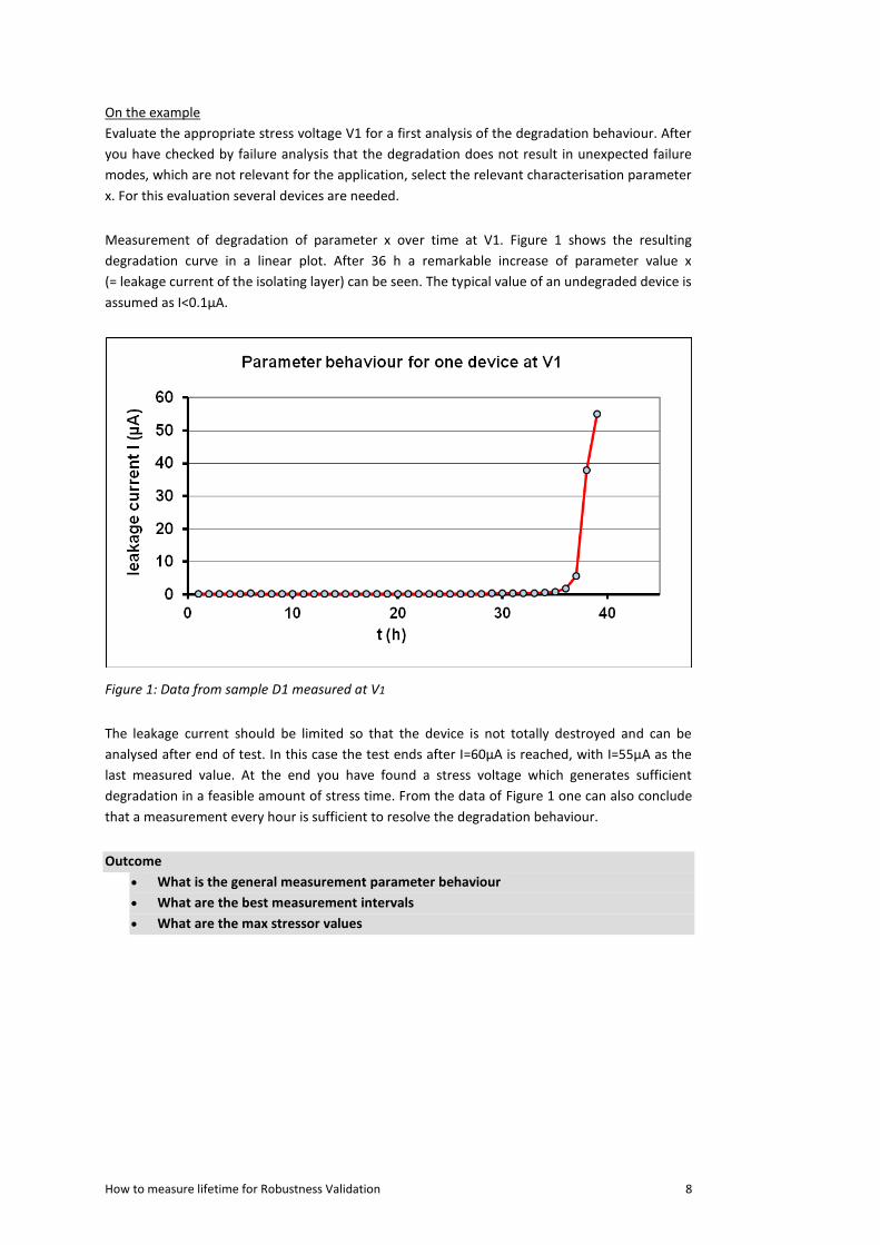
On the example

Evaluate the appropriate stress voltage V1 for a first analysis of the degradation behaviour. After

you have checked by failure analysis that the degradation does not result in unexpected failure

modes, which are not relevant for the application, select the relevant characterisation parameter

x. For this evaluation several devices are needed.

Measurement of degradation of parameter x over time at V1. Figure 1 shows the resulting

degradation curve in a linear plot. After 36 h a remarkable increase of parameter value x

(= leakage current of the isolating layer) can be seen. The typical value of an undegraded device is

assumed as I<0.1µA.

Figure 1: Data from sample D1 measured at V1

The leakage current should be limited so that the device is not totally destroyed and can be

analysed after end of test. In this case the test ends after I=60µA is reached, with I=55µA as the

last measured value. At the end you have found a stress voltage which generates sufficient

degradation in a feasible amount of stress time. From the data of Figure 1 one can also conclude

that a measurement every hour is sufficient to resolve the degradation behaviour.

Outcome

What is the general measurement parameter behaviour

What are the best measurement intervals

What are the max stressor values


3. Performing investigation on several devices

Topic: Defining the complete test setup and performing the test

After having gained a typical product behaviour due to a stress-parameter by doing a pre-

evaluation you can do the investigations on a higher number of samples. This will result in a

better characterisation of the product and its statistical behaviour. Not every part degrades in the

same way. There is some part to part variation, which is extremely important to characterise the

product, e.g. defining the lifetime t63 and the Weibull slope β.

Definition of sample size

The sample size must not be too small. This would result in reduced data accuracy or broad

confidence range.

On the other hand the sample size should not be too high as the information gained will not

linearly increase with sample size. So depending on the exact situation a 10x higher sample size

will only double data accuracy. Increase sample will also increase the testing costs requiring a

sound cost-benefit-ratio.

So the answer on the question „What is the right sample size?“ cannot be given in general. In any

case it must be large enough to characterize the behaviour. If it turns out that it is too small

additional samples have to be taken.

On the example

In this case the test is started with the sample size 16 (usually there is some experience existing

which sample size is appropriate, with the assumption that these are sufficient for the

investigations, at the end of the experiment it will show up if this sample size was the right one).

Each device is labelled with a number from D1 to D16.

The stress conditions are the same as for the pre-evaluation and are defined as:

Stress voltage: V1

t meas,max = 40 h

fmeas = 1h-1

Imax = 60µA

Remark: Imax = 60µA is not the failure criterion. This is the maximum current which is detected.

This may be caused by limitation of the measurement tool, the device itself etc. It is the value up

to which the current is logged.

Under these conditions the rest of the complete sample of 16 devices D2-D16 is measured and

the results transferred to the data base (see Table 1). For each device the parameter x is

measured with a frequency of 1 hour - starting with the first data point after 1 h of constant

voltage stress. A rough check of the data shows that the devices behave slightly different.

Most of the devices reach the current-limit within the timeframe of 40 h, but for D12 the

degradation after 40 h is only I=25 µA.


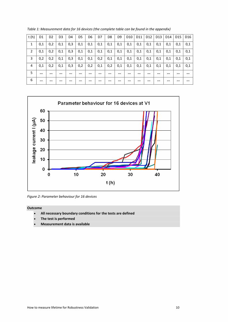
Table 1: Measurement data for 16 devices (the complete table can be found in the appendix)

t (h) D1 D2 D3 D4 D5 D6 D7 D8 D9 D10 D11 D12 D13 D14 D15 D16

1 0,1 0,2 0,1 0,3 0,1 0,1 0,1 0,1 0,1 0,1 0,1 0,1 0,1 0,1 0,1 0,1

2 0,1 0,2 0,1 0,3 0,1 0,1 0,1 0,1 0,1 0,1 0,1 0,1 0,1 0,1 0,1 0,1

3 0,2 0,2 0,1 0,3 0,1 0,1 0,2 0,1 0,1 0,1 0,1 0,1 0,1 0,1 0,1 0,1

4 0,1 0,2 0,1 0,3 0,2 0,2 0,1 0,2 0,1 0,1 0,1 0,1 0,1 0,1 0,1 0,1

5 ... ... ... ... ... ... ... ... ... ... ... ... ... ... ... ...

6 ... ... ... ... ... ... ... ... ... ... ... ... ... ... ... ...

Figure 2: Parameter behaviour for 16 devices

Outcome

All necessary boundary conditions for the tests are defined

The test is performed

Measurement data is available


4. Generating a lifetime distribution

Topic: analysing data to get to a lifetime distribution

The above graph shows the change of the leakage current over time. Up to now the failure

criterion is not determined, the value which separates well from defective devices.

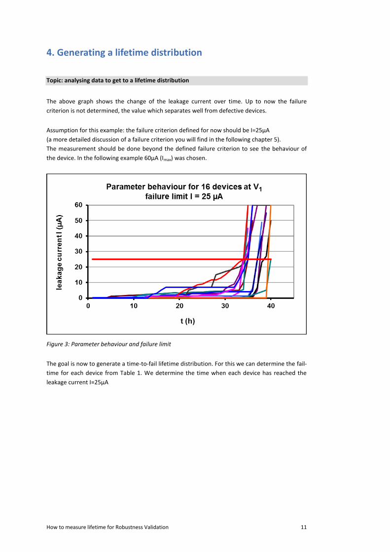
Assumption for this example: the failure criterion defined for now should be I=25µA

(a more detailed discussion of a failure criterion you will find in the following chapter 5).

The measurement should be done beyond the defined failure criterion to see the behaviour of

the device. In the following example 60µA (Imax) was chosen.

Figure 3: Parameter behaviour and failure limit

The goal is now to generate a time-to-fail lifetime distribution. For this we can determine the fail-

time for each device from Table 1. We determine the time when each device has reached the

leakage current I=25µA


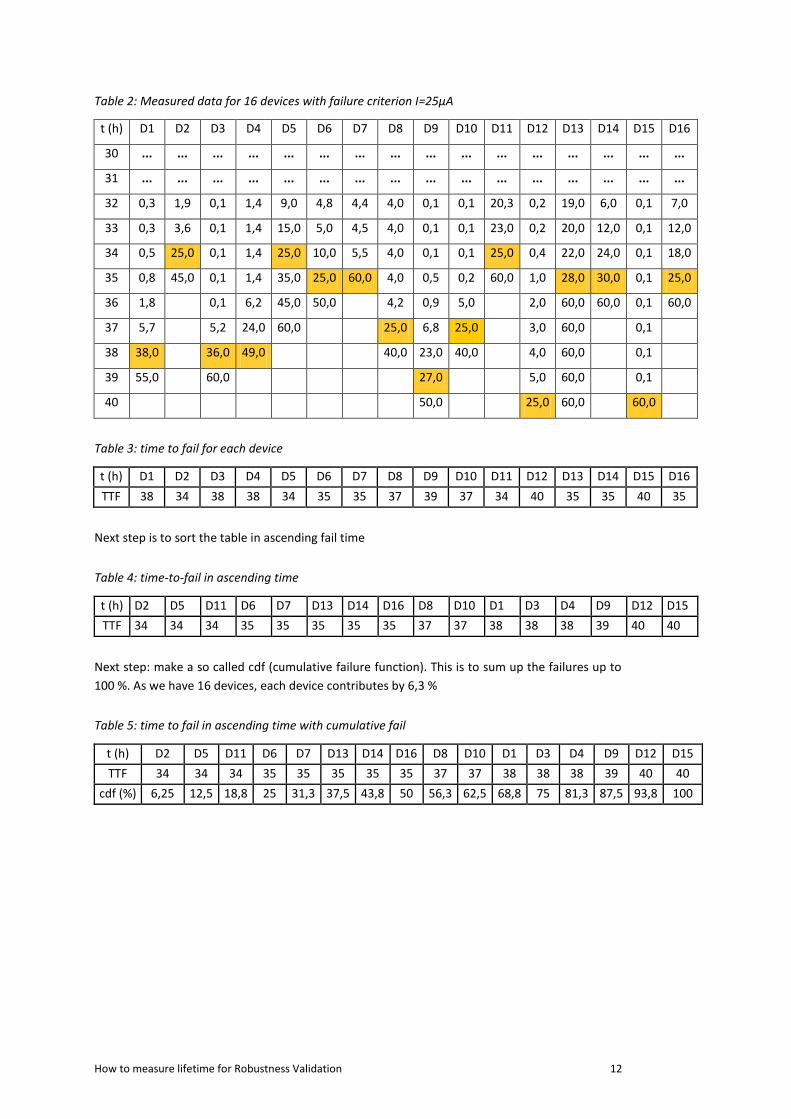
Table 2: Measured data for 16 devices with failure criterion I=25µA


30 ... ... ... ... ... ... ... ... ... ... ... ... ... ... ... ...

31 ... ... ... ... ... ... ... ... ... ... ... ... ... ... ... ...

32 0,3 1,9 0,1 1,4 9,0 4,8 4,4 4,0 0,1 0,1 20,3 0,2 19,0 6,0 0,1 7,0

33 0,3 3,6 0,1 1,4 15,0 5,0 4,5 4,0 0,1 0,1 23,0 0,2 20,0 12,0 0,1 12,0

34 0,5 25,0 0,1 1,4 25,0 10,0 5,5 4,0 0,1 0,1 25,0 0,4 22,0 24,0 0,1 18,0

35 0,8 45,0 0,1 1,4 35,0 25,0 60,0 4,0 0,5 0,2 60,0 1,0 28,0 30,0 0,1 25,0

36 1,8 0,1 6,2 45,0 50,0 4,2 0,9 5,0 2,0 60,0 60,0 0,1 60,0

37 5,7 5,2 24,0 60,0 25,0 6,8 25,0 3,0 60,0 0,1

38 38,0 36,0 49,0 40,0 23,0 40,0 4,0 60,0 0,1

39 55,0 60,0 27,0 5,0 60,0 0,1

40 50,0 25,0 60,0 60,0

Table 3: time to fail for each device


TTF 38 34 38 38 34 35 35 37 39 37 34 40 35 35 40 35

Next step is to sort the table in ascending fail time

Table 4: time-to-fail in ascending time


TTF 34 34 34 35 35 35 35 35 37 37 38 38 38 39 40 40

Next step: make a so called cdf (cumulative failure function). This is to sum up the failures up to

100 %. As we have 16 devices, each device contributes by 6,3 %

Table 5: time to fail in ascending time with cumulative fail


TTF 34 34 34 35 35 35 35 35 37 37 38 38 38 39 40 40

cdf (%) 6,25 12,5 18,8 25 31,3 37,5 43,8 50 56,3 62,5 68,8 75 81,3 87,5 93,8 100


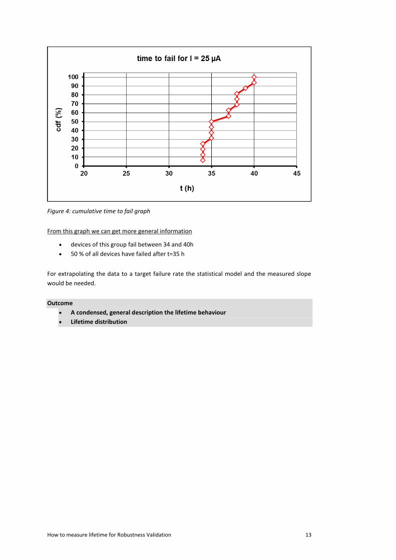
Figure 4: cumulative time to fail graph

From this graph we can get more general information

devices of this group fail between 34 and 40h

50 % of all devices have failed after t=35 h

For extrapolating the data to a target failure rate the statistical model and the measured slope

would be needed.

Outcome

A condensed, general description the lifetime behaviour

Lifetime distribution


5. Defining the failure criterion

Topic: defining the failure criteria

„What is a failure?“ To answer that question we need to have a criterion – the failure criterion.

But what is a failure? Looking at the common definition of a failure we get

a state of inability to perform a normal function (Merriam-Webster)

non-performance of something due, required, or expected (Dictionary.com)

The inability of a system or system component to perform a required function within

specified limits. (learn that)

This means that the criterion when degradation becomes a failure has to be defined based on the

specification, the application or customer requirements. In some cases a different failure

criterion can result in a different failure distribution and therefore different lifetime.

To demonstrate the effect of different failure criteria an example with three cases is generated.

The three criteria are:

Ifail = 1µA

Ifail = 5µA

Ifail l = 25µA

We get for the time to fail

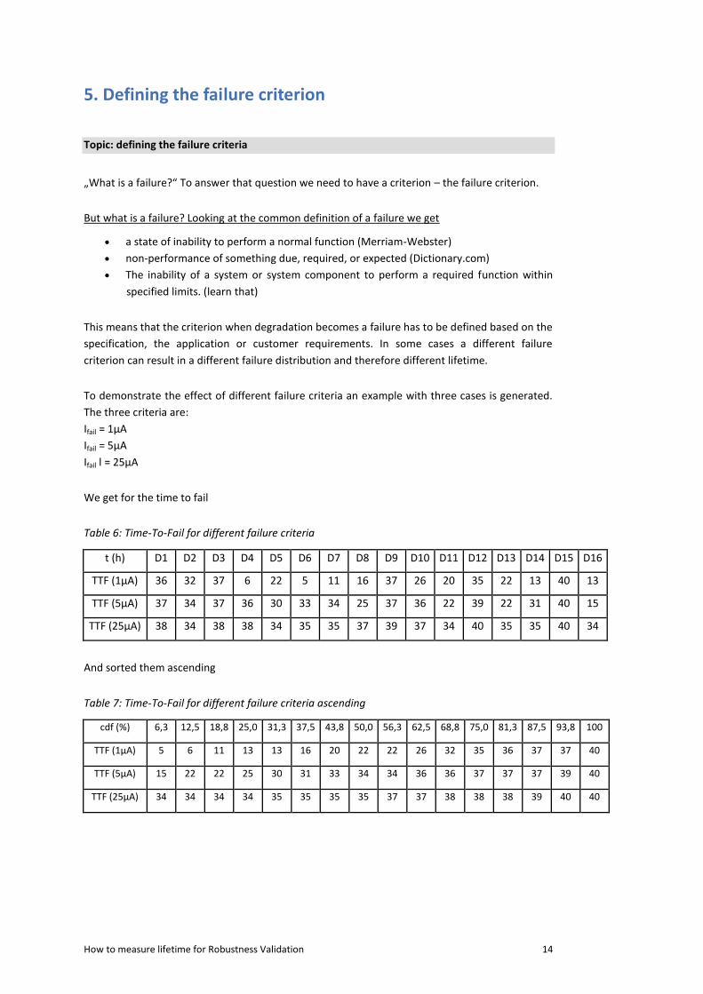
Table 6: Time-To-Fail for different failure criteria


TTF (1µA) 36 32 37 6 22 5 11 16 37 26 20 35 22 13 40 13

TTF (5µA) 37 34 37 36 30 33 34 25 37 36 22 39 22 31 40 15

TTF (25µA) 38 34 38 38 34 35 35 37 39 37 34 40 35 35 40 34

And sorted them ascending

Table 7: Time-To-Fail for different failure criteria ascending

cdf (%) 6,3 12,5 18,8 25,0 31,3 37,5 43,8 50,0 56,3 62,5 68,8 75,0 81,3 87,5 93,8 100

TTF (1µA) 5 6 11 13 13 16 20 22 22 26 32 35 36 37 37 40

TTF (5µA) 15 22 22 25 30 31 33 34 34 36 36 37 37 37 39 40

TTF (25µA) 34 34 34 34 35 35 35 35 37 37 38 38 38 39 40 40


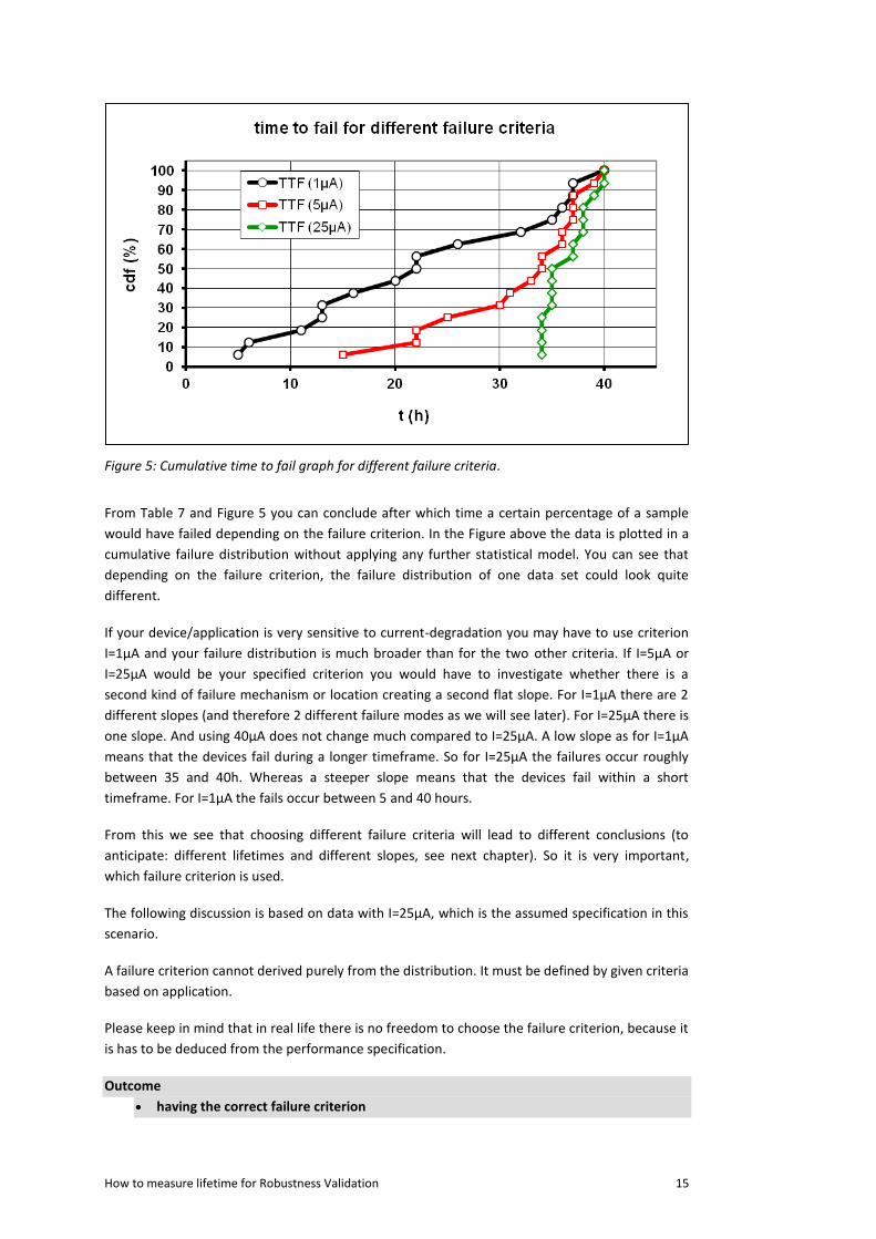
Figure 5: Cumulative time to fail graph for different failure criteria.

From Table 7 and Figure 5 you can conclude after which time a certain percentage of a sample

would have failed depending on the failure criterion. In the Figure above the data is plotted in a

cumulative failure distribution without applying any further statistical model. You can see that

depending on the failure criterion, the failure distribution of one data set could look quite

different.

If your device/application is very sensitive to current-degradation you may have to use criterion

I=1µA and your failure distribution is much broader than for the two other criteria. If I=5µA or

I=25µA would be your specified criterion you would have to investigate whether there is a

second kind of failure mechanism or location creating a second flat slope. For I=1µA there are 2

different slopes (and therefore 2 different failure modes as we will see later). For I=25µA there is

one slope. And using 40µA does not change much compared to I=25µA. A low slope as for I=1µA

means that the devices fail during a longer timeframe. So for I=25µA the failures occur roughly

between 35 and 40h. Whereas a steeper slope means that the devices fail within a short

timeframe. For I=1µA the fails occur between 5 and 40 hours.

From this we see that choosing different failure criteria will lead to different conclusions (to

anticipate: different lifetimes and different slopes, see next chapter). So it is very important,

which failure criterion is used.

The following discussion is based on data with I=25µA, which is the assumed specification in this

scenario.

A failure criterion cannot derived purely from the distribution. It must be defined by given criteria

based on application.

Please keep in mind that in real life there is no freedom to choose the failure criterion, because it

is has to be deduced from the performance specification.

Outcome

having the correct failure criterion


6. Evaluating the lifetime distribution parameters

Topic: how to characterise a life time distribution

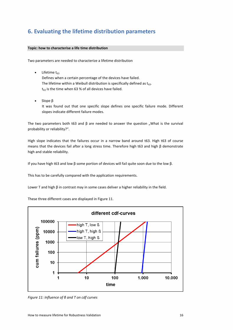
Two parameters are needed to characterize a lifetime distribution

Lifetime t63

Defines when a certain percentage of the devices have failed.

The lifetime within a Weibull distribution is specifically defined as t63.

t63 is the time when 63 % of all devices have failed.

Slope β

It was found out that one specific slope defines one specific failure mode. Different

slopes indicate different failure modes.

The two parameters both t63 and β are needed to answer the question „What is the survival

probability or reliability?“.

High slope indicates that the failures occur in a narrow band around t63. High t63 of course

means that the devices fail after a long stress time. Therefore high t63 and high β demonstrate

high and stable reliability.

If you have high t63 and low β some portion of devices will fail quite soon due to the low β.

This has to be carefully compared with the application requirements.

Lower T and high β in contrast may in some cases deliver a higher reliability in the field.

These three different cases are displayed in Figure 11.

Figure 11: Influence of β and T on cdf curves


Bathtub curve

Weibull diagram

time

cum

failures early life

extrinsic fails

ß<1

useful life

random fails

ß=1

wear out

intrinsic fails

ß>1

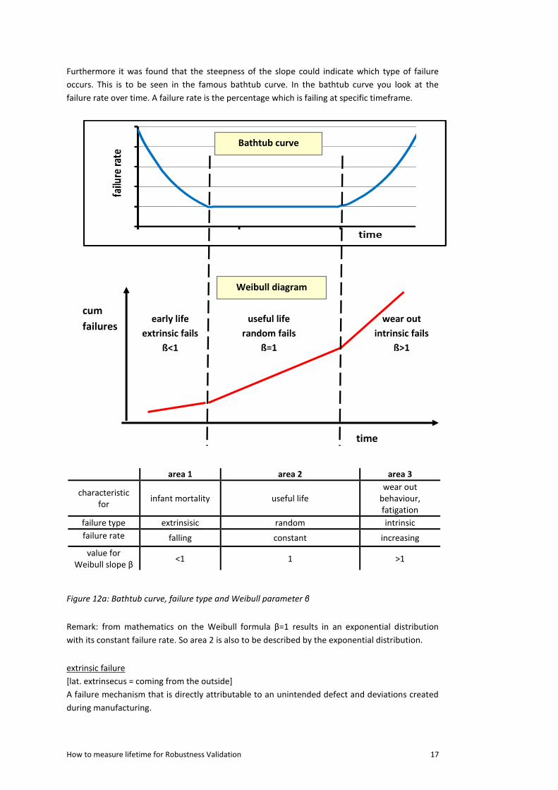
Furthermore it was found that the steepness of the slope could indicate which type of failure

occurs. This is to be seen in the famous bathtub curve. In the bathtub curve you look at the

failure rate over time. A failure rate is the percentage which is failing at specific timeframe.

area 1 area 2 area 3

characteristic for

infant mortality useful life wear out

behaviour, fatigation

failure type extrinsisic random intrinsic

failure rate falling constant increasing

value for Weibull slope β

<1 1 >1

Figure 12a: Bathtub curve, failure type and Weibull parameter β

Remark: from mathematics on the Weibull formula β=1 results in an exponential distribution

with its constant failure rate. So area 2 is also to be described by the exponential distribution.

extrinsic failure

[lat. extrinsecus = coming from the outside]

A failure mechanism that is directly attributable to an unintended defect and deviations created

during manufacturing.


Intrinsic failure

[lat., intrinsecus = inside]

A failure mechanism attributable to natural deterioration of materials processed. These failures

are correlated to the intended selection of material, process technology and design.

For further definitions see [ 3]

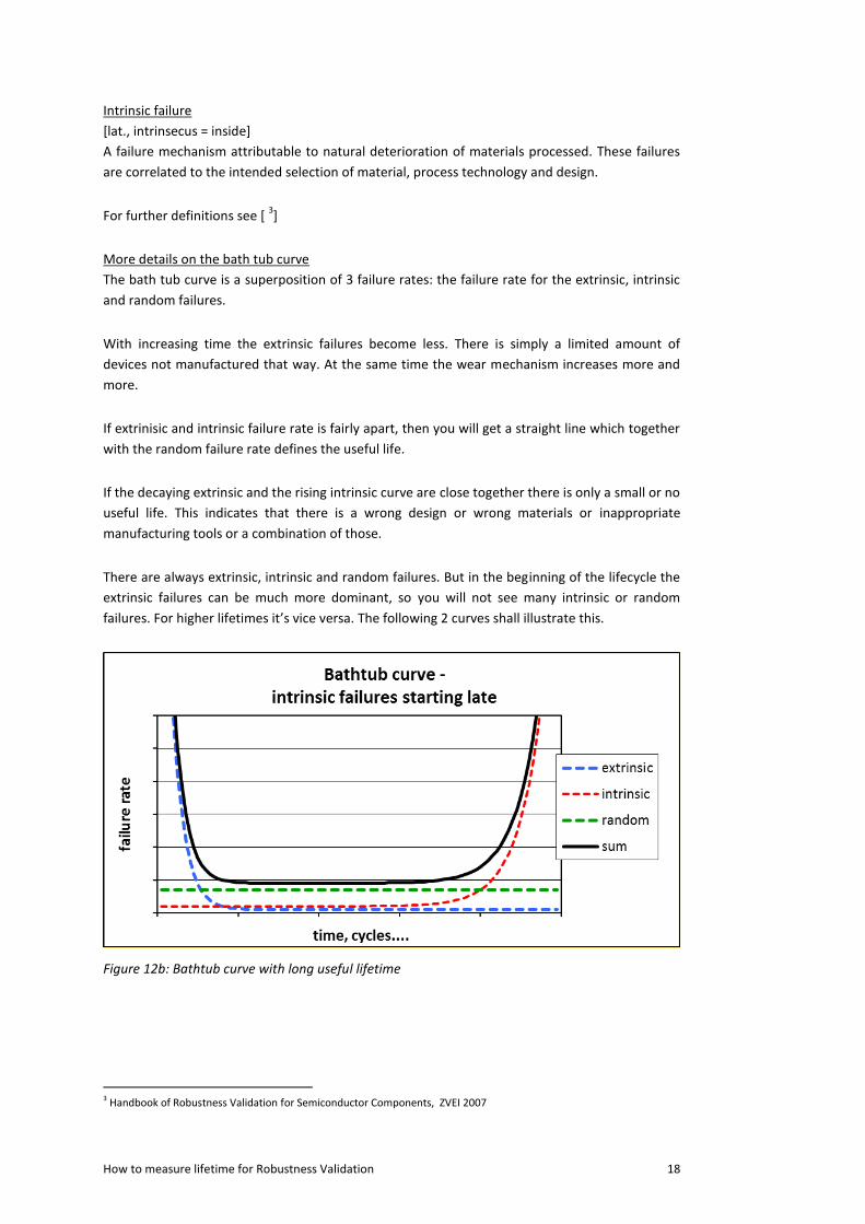
More details on the bath tub curve

The bath tub curve is a superposition of 3 failure rates: the failure rate for the extrinsic, intrinsic

and random failures.

With increasing time the extrinsic failures become less. There is simply a limited amount of

devices not manufactured that way. At the same time the wear mechanism increases more and

more.

If extrinisic and intrinsic failure rate is fairly apart, then you will get a straight line which together

with the random failure rate defines the useful life.

If the decaying extrinsic and the rising intrinsic curve are close together there is only a small or no

useful life. This indicates that there is a wrong design or wrong materials or inappropriate

manufacturing tools or a combination of those.

There are always extrinsic, intrinsic and random failures. But in the beginning of the lifecycle the

extrinsic failures can be much more dominant, so you will not see many intrinsic or random

failures. For higher lifetimes it’s vice versa. The following 2 curves shall illustrate this.

Figure 12b: Bathtub curve with long useful lifetime

3 Handbook of Robustness Validation for Semiconductor Components, ZVEI 2007


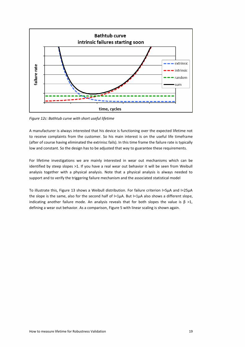
Figure 12c: Bathtub curve with short useful lifetime

A manufacturer is always interested that his device is functioning over the expected lifetime not

to receive complaints from the customer. So his main interest is on the useful life timeframe

(after of course having eliminated the extrinisc fails). In this time frame the failure rate is typically

low and constant. So the design has to be adjusted that way to guarantee these requirements.

For lifetime investigations we are mainly interested in wear out mechanisms which can be

identified by steep slopes >1. If you have a real wear out behavior it will be seen from Weibull

analysis together with a physical analysis. Note that a physical analysis is always needed to

support and to verify the triggering failure mechanism and the associated statistical model

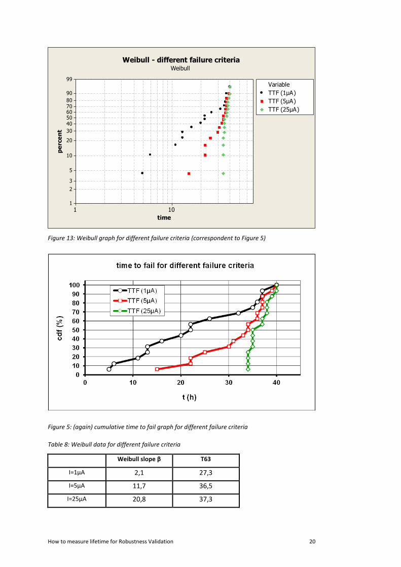
To illustrate this, Figure 13 shows a Weibull distribution. For failure criterion I=5µA and I=25µA

the slope is the same, also for the second half of I=1µA. But I=1µA also shows a different slope,

indicating another failure mode. An analysis reveals that for both slopes the value is β >1,

defining a wear out behavior. As a comparison, Figure 5 with linear scaling is shown again.


101

99

90

8070605040

30

20

10

5

3

2

1

time

pe

rce

nt

TTF (1µA)

TTF (5µA)

TTF (25µA)

Variable

Weibull

Weibull - different failure criteria

Figure 13: Weibull graph for different failure criteria (correspondent to Figure 5)

Figure 5: (again) cumulative time to fail graph for different failure criteria

Table 8: Weibull data for different failure criteria

Weibull slope β T63

I=1µA 2,1 27,3

I=5µA 11,7 36,5

I=25µA 20,8 37,3


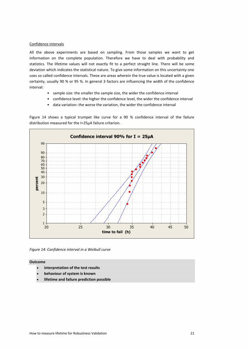
Confidence intervals

All the above experiments are based on sampling. From those samples we want to get

information on the complete population. Therefore we have to deal with probability and

statistics. The lifetime values will not exactly fit to a perfect straight line. There will be some

deviation which indicates the statistical nature. To give some information on this uncertainty one

uses so called confidence intervals. These are areas wherein the true value is located with a given

certainty, usually 90 % or 95 %. In general 3 factors are influencing the width of the confidence

interval:

• sample size: the smaller the sample size, the wider the confidence interval

• confidence level: the higher the confidence level, the wider the confidence interval

• data variation: the worse the variation, the wider the confidence interval

Figure 14 shows a typical trumpet like curve for a 90 % confidence interval of the failure

distribution measured for the I=25µA failure criterion.

50454035302520

99

90

8070605040

30

20

10

5

3

2

1

time to fail (h)

pe

rce

nt

Confidence interval 90% for I = 25µA

Figure 14: Confidence interval in a Weibull curve

Outcome

interpretation of the test results

behaviour of system is known

lifetime and failure prediction possible


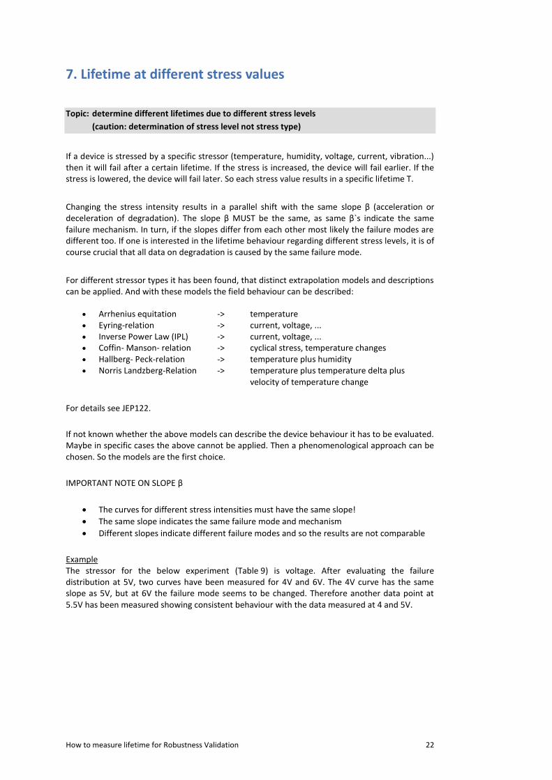
7. Lifetime at different stress values

Topic: determine different lifetimes due to different stress levels

(caution: determination of stress level not stress type)

If a device is stressed by a specific stressor (temperature, humidity, voltage, current, vibration...) then it will fail after a certain lifetime. If the stress is increased, the device will fail earlier. If the stress is lowered, the device will fail later. So each stress value results in a specific lifetime T.

Changing the stress intensity results in a parallel shift with the same slope β (acceleration or deceleration of degradation). The slope β MUST be the same, as same β`s indicate the same failure mechanism. In turn, if the slopes differ from each other most likely the failure modes are different too. If one is interested in the lifetime behaviour regarding different stress levels, it is of course crucial that all data on degradation is caused by the same failure mode.

For different stressor types it has been found, that distinct extrapolation models and descriptions can be applied. And with these models the field behaviour can be described:

Arrhenius equitation -> temperature Eyring-relation -> current, voltage, ... Inverse Power Law (IPL) -> current, voltage, ... Coffin- Manson- relation -> cyclical stress, temperature changes Hallberg- Peck-relation -> temperature plus humidity Norris Landzberg-Relation -> temperature plus temperature delta plus

velocity of temperature change

For details see JEP122.

If not known whether the above models can describe the device behaviour it has to be evaluated. Maybe in specific cases the above cannot be applied. Then a phenomenological approach can be chosen. So the models are the first choice.

IMPORTANT NOTE ON SLOPE β

The curves for different stress intensities must have the same slope!

The same slope indicates the same failure mode and mechanism

Different slopes indicate different failure modes and so the results are not comparable

Example The stressor for the below experiment (Table 9) is voltage. After evaluating the failure distribution at 5V, two curves have been measured for 4V and 6V. The 4V curve has the same slope as 5V, but at 6V the failure mode seems to be changed. Therefore another data point at 5.5V has been measured showing consistent behaviour with the data measured at 4 and 5V.


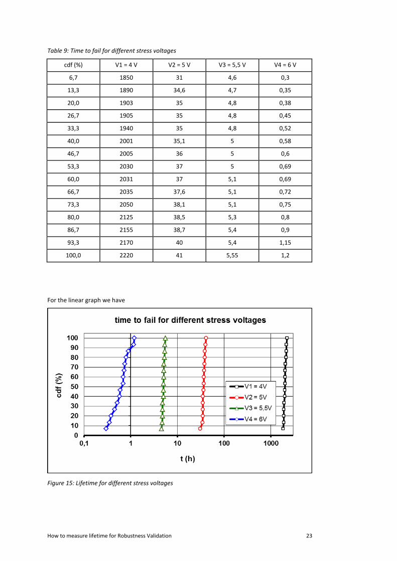
Table 9: Time to fail for different stress voltages

cdf (%) V1 = 4 V V2 = 5 V V3 = 5,5 V V4 = 6 V

6,7 1850 31 4,6 0,3

13,3 1890 34,6 4,7 0,35

20,0 1903 35 4,8 0,38

26,7 1905 35 4,8 0,45

33,3 1940 35 4,8 0,52

40,0 2001 35,1 5 0,58

46,7 2005 36 5 0,6

53,3 2030 37 5 0,69

60,0 2031 37 5,1 0,69

66,7 2035 37,6 5,1 0,72

73,3 2050 38,1 5,1 0,75

80,0 2125 38,5 5,3 0,8

86,7 2155 38,7 5,4 0,9

93,3 2170 40 5,4 1,15

100,0 2220 41 5,55 1,2

For the linear graph we have

Figure 15: Lifetime for different stress voltages


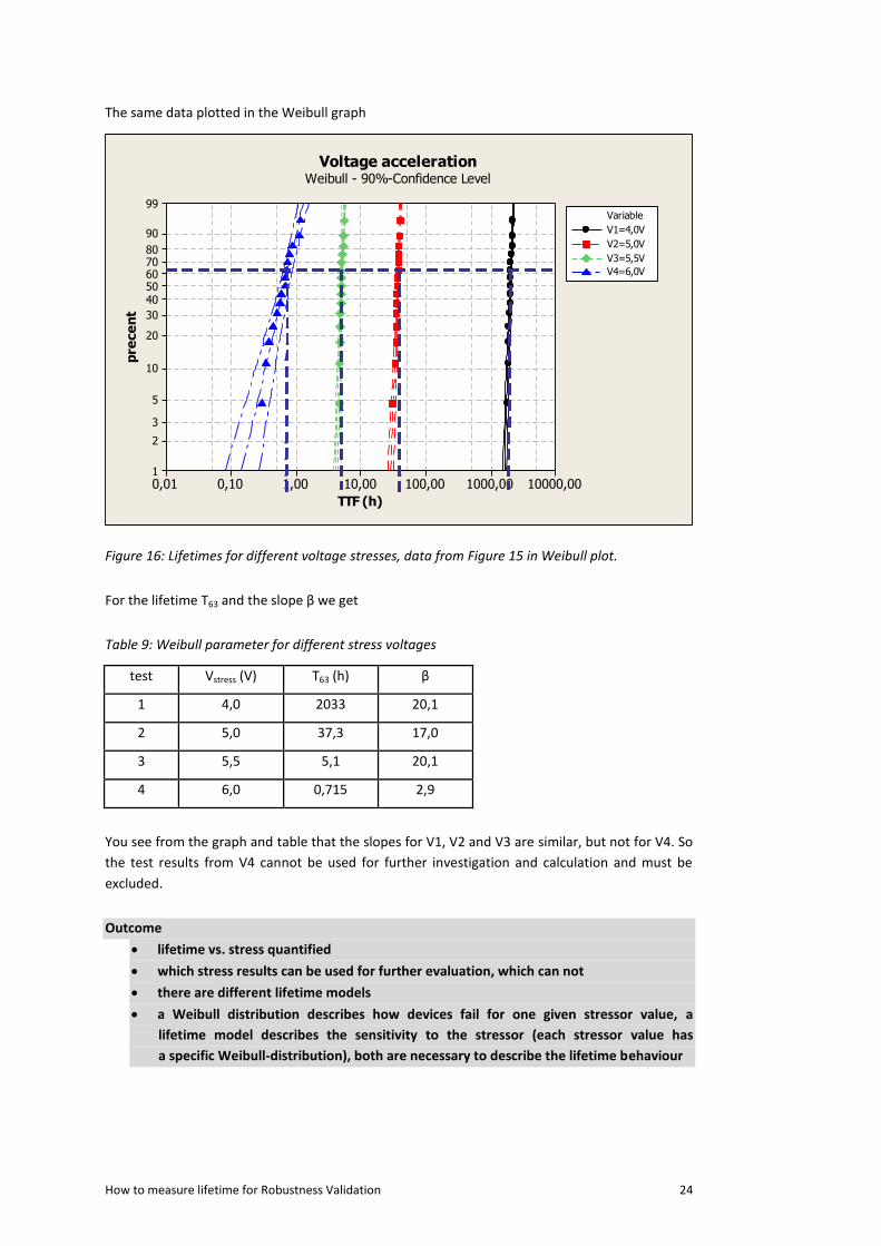
The same data plotted in the Weibull graph

Figure 16: Lifetimes for different voltage stresses, data from Figure 15 in Weibull plot.

For the lifetime T63 and the slope β we get

Table 9: Weibull parameter for different stress voltages

test Vstress (V) T63 (h) β

1 4,0 2033 20,1

2 5,0 37,3 17,0

3 5,5 5,1 20,1

4 6,0 0,715 2,9

You see from the graph and table that the slopes for V1, V2 and V3 are similar, but not for V4. So

the test results from V4 cannot be used for further investigation and calculation and must be

excluded.

Outcome

lifetime vs. stress quantified

which stress results can be used for further evaluation, which can not

there are different lifetime models

a Weibull distribution describes how devices fail for one given stressor value, a

lifetime model describes the sensitivity to the stressor (each stressor value has

a specific Weibull-distribution), both are necessary to describe the lifetime behaviour

10000,001000,00100,0010,001,000,100,01

99

90

8070605040

30

20

10

5

3

2

1

TTF (h)

pre

ce

nt

V1=4,0V

V2=5,0V

V3=5,5V

V4=6,0V

Variable

Voltage accelerationWeibull - 90%-Confidence Level


8. Applying the acceleration model

Topic: What is the correct lifetime model for the experiments?

The next step is to choose a lifetime model. This is already known from basic investigations using generic devices or first choice to deal with.

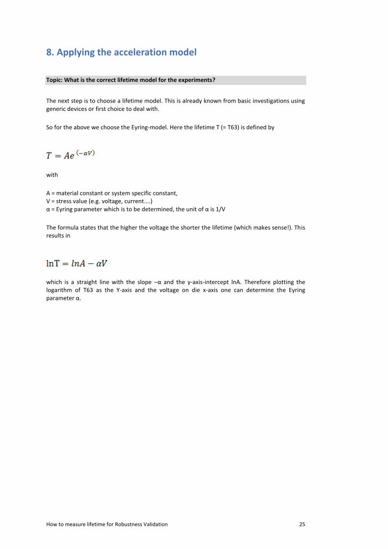
So for the above we choose the Eyring-model. Here the lifetime T (= T63) is defined by

with

A = material constant or system specific constant, V = stress value (e.g. voltage, current....) α = Eyring parameter which is to be determined, the unit of α is 1/V

The formula states that the higher the voltage the shorter the lifetime (which makes sense!). This results in

which is a straight line with the slope –α and the y-axis-intercept lnA. Therefore plotting the logarithm of T63 as the Y-axis and the voltage on die x-axis one can determine the Eyring parameter α.


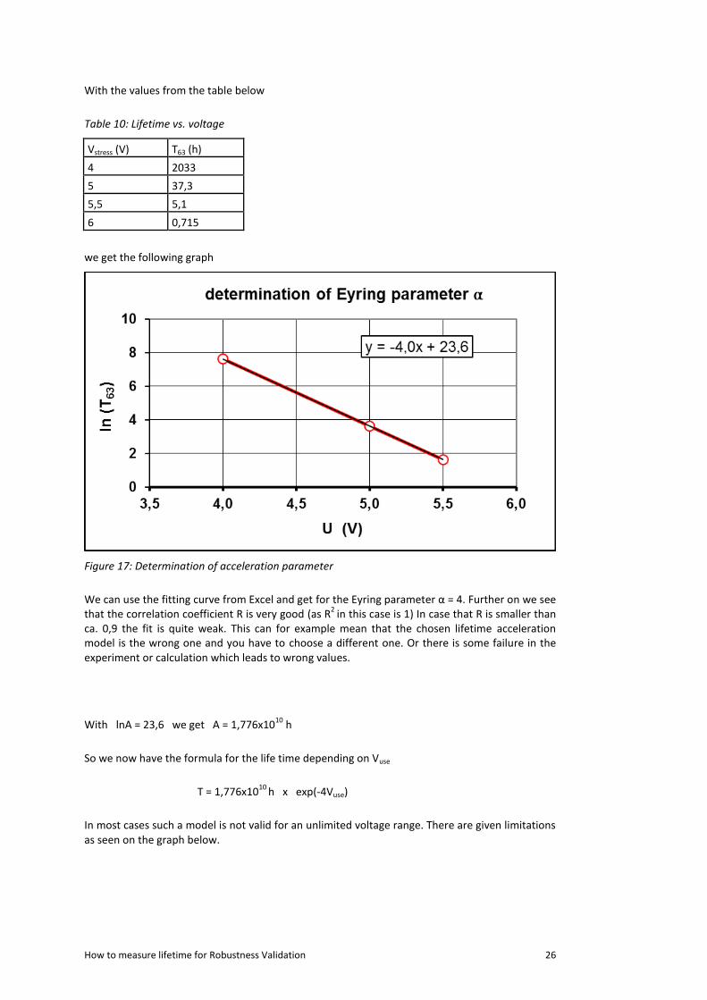
With the values from the table below

Table 10: Lifetime vs. voltage

Vstress (V) T63 (h)

4 2033

5 37,3

5,5 5,1

6 0,715

we get the following graph

Figure 17: Determination of acceleration parameter

We can use the fitting curve from Excel and get for the Eyring parameter α = 4. Further on we see that the correlation coefficient R is very good (as R

2 in this case is 1) In case that R is smaller than

ca. 0,9 the fit is quite weak. This can for example mean that the chosen lifetime acceleration model is the wrong one and you have to choose a different one. Or there is some failure in the experiment or calculation which leads to wrong values.

With lnA = 23,6 we get A = 1,776x1010

h

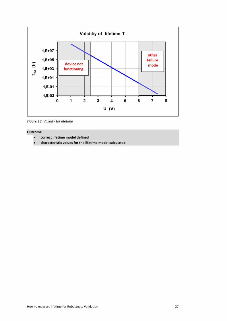
So we now have the formula for the life time depending on Vuse

T = 1,776x1010

h x exp(-4Vuse)

In most cases such a model is not valid for an unlimited voltage range. There are given limitations as seen on the graph below.


Figure 18: Validity for lifetime

Outcome

correct lifetime model defined

characteristic values for the lifetime model calculated


9. Calculating the lifetime in the field

Topic: How to determine life time in the field with the data gained so far?

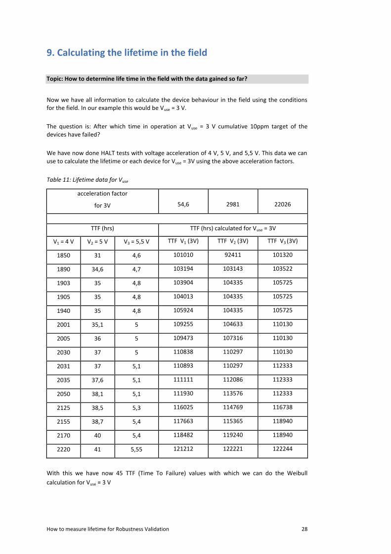
Now we have all information to calculate the device behaviour in the field using the conditions for the field. In our example this would be Vuse = 3 V.

The question is: After which time in operation at Vuse = 3 V cumulative 10ppm target of the devices have failed?

We have now done HALT tests with voltage acceleration of 4 V, 5 V, and 5,5 V. This data we can use to calculate the lifetime or each device for Vuse = 3V using the above acceleration factors.

Table 11: Lifetime data for Vuse

acceleration factor

for 3V 54,6 2981 22026

TTF (hrs) TTF (hrs) calculated for Vuse = 3V

V1 = 4 V V2 = 5 V V3 = 5,5 V TTF V1 (3V) TTF V2 (3V) TTF V3 (3V)

1850 31 4,6 101010 92411 101320

1890 34,6 4,7 103194 103143 103522

1903 35 4,8 103904 104335 105725

1905 35 4,8 104013 104335 105725

1940 35 4,8 105924 104335 105725

2001 35,1 5 109255 104633 110130

2005 36 5 109473 107316 110130

2030 37 5 110838 110297 110130

2031 37 5,1 110893 110297 112333

2035 37,6 5,1 111111 112086 112333

2050 38,1 5,1 111930 113576 112333

2125 38,5 5,3 116025 114769 116738

2155 38,7 5,4 117663 115365 118940

2170 40 5,4 118482 119240 118940

2220 41 5,55 121212 122221 122244

With this we have now 45 TTF (Time To Failure) values with which we can do the Weibull

calculation for Vuse = 3 V


1400001300001200001100001000009000080000

99,9

99

90807060504030

20

10

5

3

2

1

TTF (h)

pe

rce

nt

Form 18,72

Skala 113230

N 45

Time to fail (TTF) calculated for Vuse = 3VConfidence interval 90%

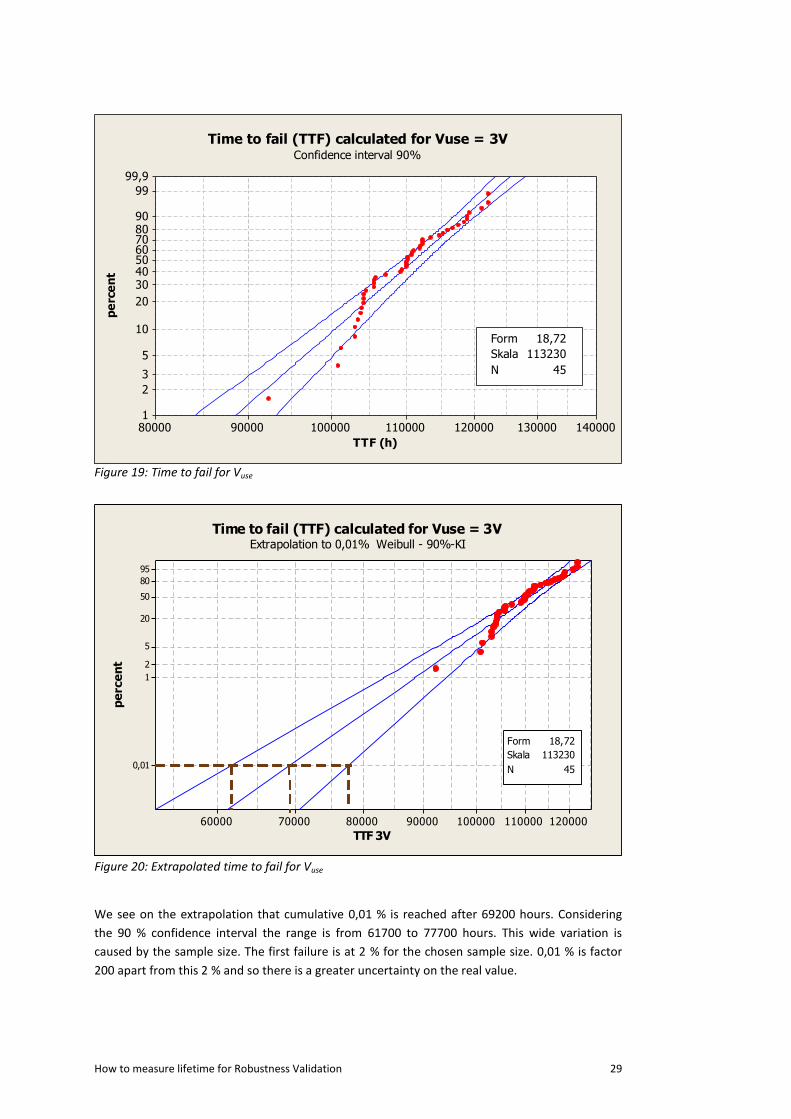
Figure 19: Time to fail for Vuse

12000011000010000090000800007000060000

95

80

50

20

5

2

1

0,01

TTF 3V

pe

rce

nt

Form 18,72

Skala 113230

N 45

Time to fail (TTF) calculated for Vuse = 3VExtrapolation to 0,01% Weibull - 90%-KI

Figure 20: Extrapolated time to fail for Vuse

We see on the extrapolation that cumulative 0,01 % is reached after 69200 hours. Considering

the 90 % confidence interval the range is from 61700 to 77700 hours. This wide variation is

caused by the sample size. The first failure is at 2 % for the chosen sample size. 0,01 % is factor

200 apart from this 2 % and so there is a greater uncertainty on the real value.


Problems and pitfalls

Using the results from the experiments one has to consider the limitations for the statements

gained. Such limitations can be imposed by the below areas

• sample size used

• how representative is the sample

• extrapolation for ppm-statements

Sample size

Accuracy is limited by sample size. The smaller the sample size, the less accurate are the results.

To find the proper sample size for the given test is the first prerequisite to avoid accuracy

limitations and a waste of time and money. Worst case the test has to be expanded with further

samples.

Representative sample

The samples used should to cover all variations and fluctuations for a process which are for

example lot to lot variations or within lot variations, tool influences.... These variations are also

related to the slope and width of the distribution, respectively.

Extrapolation

Using 50-100 samples a cumulative failure of 1 % can be identified directly. But every

extrapolation to lower failures has a certain uncertainty. This is based on the fact that you

assume the behavior of the tested devices is representative for the whole production. This,

however, is just an assumption.

Outcome

lifetime in the field calculated

can device fulfil requirements or not


10. Further Reading

For further reading on more specific questions of lifetime measurement, the following books and publications are recommended:

Practical Reliability Engineering Patrick P. O'Connor (Author), Andre Kleyner (Author) Published by Wiley ISBN-10: 047097981X ISBN-13: 978-0470979815

Handbook of Reliability Engineering& Management W. G. Ireson (Editor), ISBN-10: 007032039X ISBN-13: 978-0070320390

Accelerated Reliability Engineering: HALT and HASS G. K. Hobbs, ISBN-10: 047197966X ISBN-13: 978-0471979661

AIAG Potential Failure mode and effects Analysis FMEA (4th Edition) ISBN 978-1-60534-136-1

The New Weibull Handbook Fifth Edition, Reliability and Statistical Analysis for Predicting Life, Safety, Supportability, Risk, Cost and Warranty Claims [Spiral-bound] Dr. Robert. Abernethy (Author, Editor, Illustrator) ISBN-10: 0965306232 ISBN-13: 978-0965306232

Life cycle reliability engineering Includes bibliographical references and index. Yang, Guangbin, 1964 ISBN-13: 978-0-471-71529-0 (cloth) ISBN-10: 0-471-71529-8 (cloth)

Product reliability: specification and performance. British Library Cataloguing in Publication Data (Springer series in reliability engineering) ISBN-13: 9781848002708

Reliability Engineering Theory and Practice Fifth edition ISBN 978-3-540-49388-4 5th ed. Springer Berlin Heidelberg New York 2007

Volume 3 Part 1 Ensuring reliability of car manufacturers- Reliability Management 3rd edition 2000, VDA QMC

Accelerated testing and Validation Testing, Engineering and Management Tools for lean development Alex Porter, Elsevier 2004, ISBN 0-7506-7653-1

Reliability Physics and Engineering Time-To-Failure Modeling, JW McPherson PhD, Pherson, Springer2010, ISBN978-1-4419-6347-5

Design for reliability Dana Crowe, Alec Feinberg CRC Press 2001 ISBN 9780849311116

Reliability Physics and Engineering: Time-To-Failure Modeling, Joe McPherson, ISBN 978-1-4419-6348-2, Springer

http://www.amazon.com/s/ref=ntt_athr_dp_sr_1?_encoding=UTF8&field-author=Patrick%20P.%20O%27Connor&ie=UTF8&search-alias=books&sort=relevancerank

http://www.amazon.com/s/ref=ntt_athr_dp_sr_2?_encoding=UTF8&field-author=Andre%20Kleyner&ie=UTF8&search-alias=books&sort=relevancerank

http://www.amazon.com/s/ref=ntt_athr_dp_sr_1?_encoding=UTF8&field-author=Dr.%20Robert.%20Abernethy&ie=UTF8&search-alias=books&sort=relevancerank

http://rb-purpdm.de.bosch.com/purpdm/run?app=info/infoElements.jsp?cmd=infoElement_show&element_id=INFO86799287476637677






11. Appendix A: Strange curves – what to do?

Topic: Graph is not a straight line as expected. What is the interpretation? What has to be

done?

For the cdf graph you usually expect usually one straight line. But sometimes this is not the case

and one is encountered with deviations from such a straight line. Often these deviations are not

caused by measurement failures, but have a physical background.

CAUTION: The following discussion is qualitative. Quantitative interpretation of failure

distributions can be done using the appropriate statistical plot.

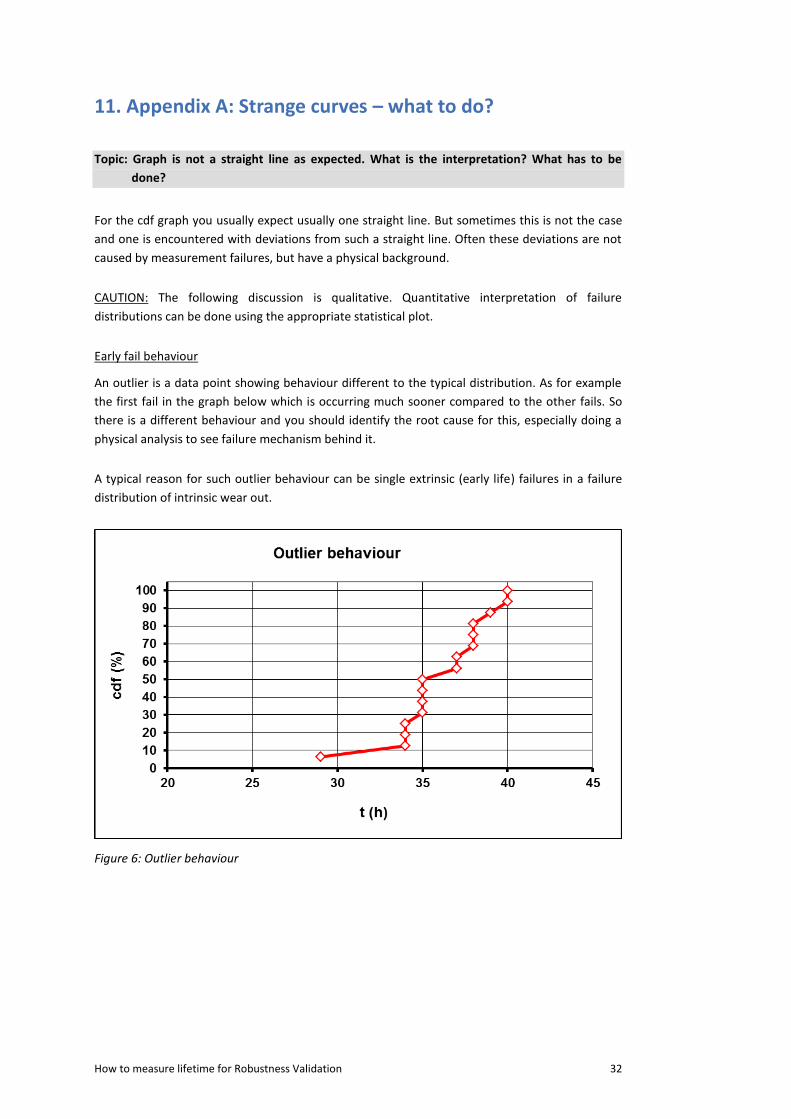
Early fail behaviour

An outlier is a data point showing behaviour different to the typical distribution. As for example

the first fail in the graph below which is occurring much sooner compared to the other fails. So

there is a different behaviour and you should identify the root cause for this, especially doing a

physical analysis to see failure mechanism behind it.

A typical reason for such outlier behaviour can be single extrinsic (early life) failures in a failure

distribution of intrinsic wear out.

Figure 6: Outlier behaviour


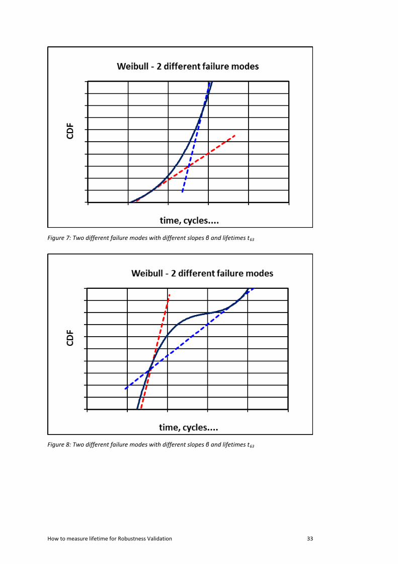
Figure 7: Two different failure modes with different slopes β and lifetimes t63

Figure 8: Two different failure modes with different slopes β and lifetimes t63


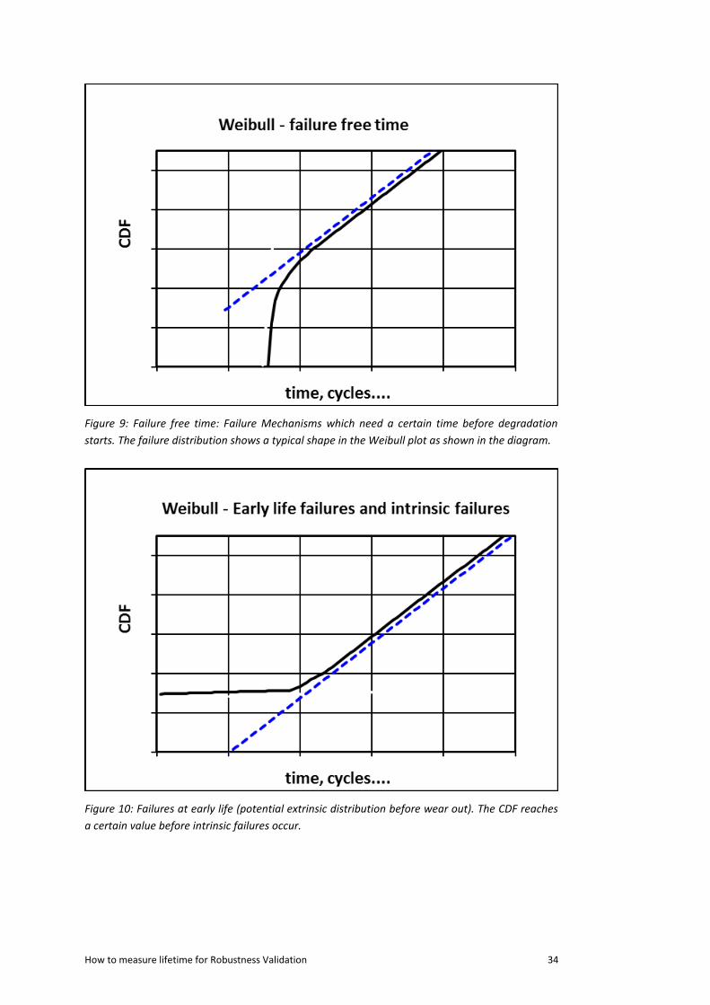
Figure 9: Failure free time: Failure Mechanisms which need a certain time before degradation

starts. The failure distribution shows a typical shape in the Weibull plot as shown in the diagram.

Figure 10: Failures at early life (potential extrinsic distribution before wear out). The CDF reaches

a certain value before intrinsic failures occur.


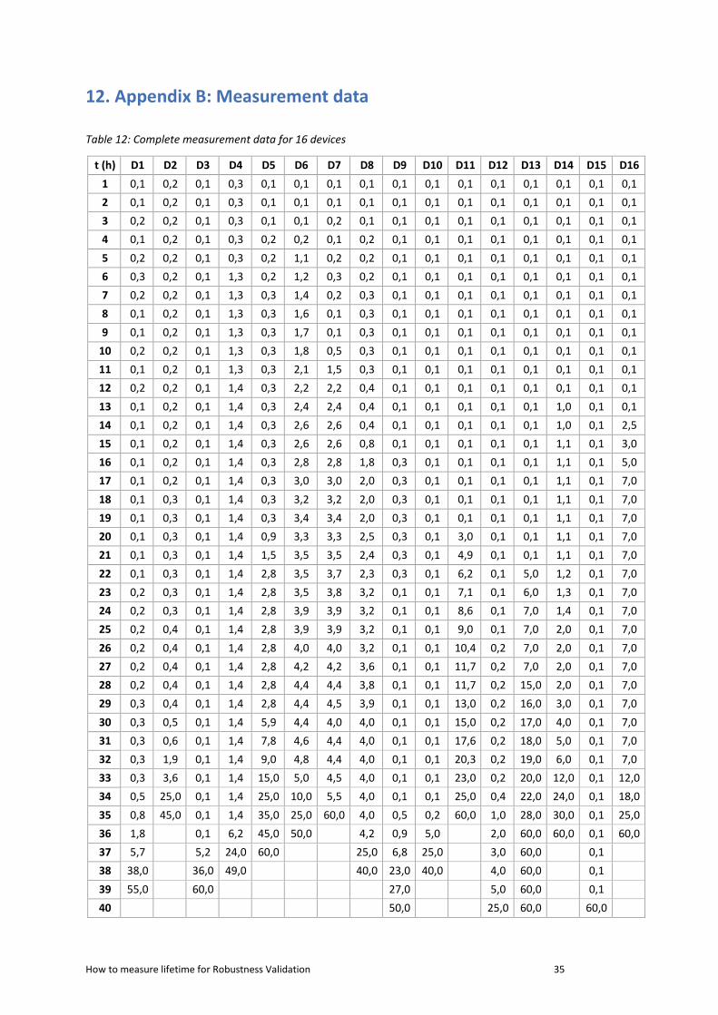
12. Appendix B: Measurement data

Table 12: Complete measurement data for 16 devices


1 0,1 0,2 0,1 0,3 0,1 0,1 0,1 0,1 0,1 0,1 0,1 0,1 0,1 0,1 0,1 0,1

2 0,1 0,2 0,1 0,3 0,1 0,1 0,1 0,1 0,1 0,1 0,1 0,1 0,1 0,1 0,1 0,1

3 0,2 0,2 0,1 0,3 0,1 0,1 0,2 0,1 0,1 0,1 0,1 0,1 0,1 0,1 0,1 0,1

4 0,1 0,2 0,1 0,3 0,2 0,2 0,1 0,2 0,1 0,1 0,1 0,1 0,1 0,1 0,1 0,1

5 0,2 0,2 0,1 0,3 0,2 1,1 0,2 0,2 0,1 0,1 0,1 0,1 0,1 0,1 0,1 0,1

6 0,3 0,2 0,1 1,3 0,2 1,2 0,3 0,2 0,1 0,1 0,1 0,1 0,1 0,1 0,1 0,1

7 0,2 0,2 0,1 1,3 0,3 1,4 0,2 0,3 0,1 0,1 0,1 0,1 0,1 0,1 0,1 0,1

8 0,1 0,2 0,1 1,3 0,3 1,6 0,1 0,3 0,1 0,1 0,1 0,1 0,1 0,1 0,1 0,1

9 0,1 0,2 0,1 1,3 0,3 1,7 0,1 0,3 0,1 0,1 0,1 0,1 0,1 0,1 0,1 0,1

10 0,2 0,2 0,1 1,3 0,3 1,8 0,5 0,3 0,1 0,1 0,1 0,1 0,1 0,1 0,1 0,1

11 0,1 0,2 0,1 1,3 0,3 2,1 1,5 0,3 0,1 0,1 0,1 0,1 0,1 0,1 0,1 0,1

12 0,2 0,2 0,1 1,4 0,3 2,2 2,2 0,4 0,1 0,1 0,1 0,1 0,1 0,1 0,1 0,1

13 0,1 0,2 0,1 1,4 0,3 2,4 2,4 0,4 0,1 0,1 0,1 0,1 0,1 1,0 0,1 0,1

14 0,1 0,2 0,1 1,4 0,3 2,6 2,6 0,4 0,1 0,1 0,1 0,1 0,1 1,0 0,1 2,5

15 0,1 0,2 0,1 1,4 0,3 2,6 2,6 0,8 0,1 0,1 0,1 0,1 0,1 1,1 0,1 3,0

16 0,1 0,2 0,1 1,4 0,3 2,8 2,8 1,8 0,3 0,1 0,1 0,1 0,1 1,1 0,1 5,0

17 0,1 0,2 0,1 1,4 0,3 3,0 3,0 2,0 0,3 0,1 0,1 0,1 0,1 1,1 0,1 7,0

18 0,1 0,3 0,1 1,4 0,3 3,2 3,2 2,0 0,3 0,1 0,1 0,1 0,1 1,1 0,1 7,0

19 0,1 0,3 0,1 1,4 0,3 3,4 3,4 2,0 0,3 0,1 0,1 0,1 0,1 1,1 0,1 7,0

20 0,1 0,3 0,1 1,4 0,9 3,3 3,3 2,5 0,3 0,1 3,0 0,1 0,1 1,1 0,1 7,0

21 0,1 0,3 0,1 1,4 1,5 3,5 3,5 2,4 0,3 0,1 4,9 0,1 0,1 1,1 0,1 7,0

22 0,1 0,3 0,1 1,4 2,8 3,5 3,7 2,3 0,3 0,1 6,2 0,1 5,0 1,2 0,1 7,0

23 0,2 0,3 0,1 1,4 2,8 3,5 3,8 3,2 0,1 0,1 7,1 0,1 6,0 1,3 0,1 7,0

24 0,2 0,3 0,1 1,4 2,8 3,9 3,9 3,2 0,1 0,1 8,6 0,1 7,0 1,4 0,1 7,0

25 0,2 0,4 0,1 1,4 2,8 3,9 3,9 3,2 0,1 0,1 9,0 0,1 7,0 2,0 0,1 7,0

26 0,2 0,4 0,1 1,4 2,8 4,0 4,0 3,2 0,1 0,1 10,4 0,2 7,0 2,0 0,1 7,0

27 0,2 0,4 0,1 1,4 2,8 4,2 4,2 3,6 0,1 0,1 11,7 0,2 7,0 2,0 0,1 7,0

28 0,2 0,4 0,1 1,4 2,8 4,4 4,4 3,8 0,1 0,1 11,7 0,2 15,0 2,0 0,1 7,0

29 0,3 0,4 0,1 1,4 2,8 4,4 4,5 3,9 0,1 0,1 13,0 0,2 16,0 3,0 0,1 7,0

30 0,3 0,5 0,1 1,4 5,9 4,4 4,0 4,0 0,1 0,1 15,0 0,2 17,0 4,0 0,1 7,0

31 0,3 0,6 0,1 1,4 7,8 4,6 4,4 4,0 0,1 0,1 17,6 0,2 18,0 5,0 0,1 7,0

32 0,3 1,9 0,1 1,4 9,0 4,8 4,4 4,0 0,1 0,1 20,3 0,2 19,0 6,0 0,1 7,0

33 0,3 3,6 0,1 1,4 15,0 5,0 4,5 4,0 0,1 0,1 23,0 0,2 20,0 12,0 0,1 12,0

34 0,5 25,0 0,1 1,4 25,0 10,0 5,5 4,0 0,1 0,1 25,0 0,4 22,0 24,0 0,1 18,0

35 0,8 45,0 0,1 1,4 35,0 25,0 60,0 4,0 0,5 0,2 60,0 1,0 28,0 30,0 0,1 25,0

36 1,8 0,1 6,2 45,0 50,0 4,2 0,9 5,0 2,0 60,0 60,0 0,1 60,0

37 5,7 5,2 24,0 60,0 25,0 6,8 25,0 3,0 60,0 0,1

38 38,0 36,0 49,0 40,0 23,0 40,0 4,0 60,0 0,1

39 55,0 60,0 27,0 5,0 60,0 0,1

40 50,0 25,0 60,0 60,0

ZVEI - German Electrical and Electronic Manufacturers‘ Association

Lyoner Straße 9

60528 Frankfurt am Main, Germany

Phone: +49 69 6302 276

Fax: +49 69 6302 407

E-mail: [email protected]

www.zvei.org

Documents

How to measure lifetime for Robustness Validation step by step