How to model a TCP-IP network using only 20 parameters

How to model a TCP/IP network using only 20 parameters

Kevin Mills, NISTCxS Study Group – November 17, 2009

visual hash of MesoNet source code from http://www.wordle.net/

Outline

• Goal – Problem – Solution• Scale Reduction: Theory and Practice• Overview of the 20 MesoNet Parameters• Parameter Explanations in 5 Categories

– Network (4 parameters)

– Sources & Receivers (4 parameters)

– User Behavior (6 parameters)

– Protocols (3 parameters)

– Simulation & Measurement Control (3 parameters)

• Discuss Simulation Resource Requirements• Future Work

Goal – Problem – Solution• Goal – compare proposed Internet congestion control

algorithms under a wide range of controlled, repeatable conditions

• Problem – real network not controllable and repeatable; test beds currently too small; most network simulation models have large search space and require infeasible memory and processing resources for large, fast networks; more tractable fluid-flow simulators are currently inaccurate

• Solution – design a reduced scale network simulation model (MesoNet) that is easy to configure and tractable to compute Joint work with Jian Yuan and Edward Schwartz

The Function ☺ of a Simulation Model

y1, …, ym = f( x1|[1,…,k], …, xn|[1,…,k] )

Response State‐Space Stimulus State‐Space

Theory – Scale Reduction in Two Parts kn

k(n‐r1)

k(n‐r1‐r2)

2(n‐r1‐r2)

2(n‐r1‐r2‐r3)

2‐levelexperiment

design

modelrestriction

factorclustering

OFF (orthogonal fractional factorial)experiment design

SCIENTIFIC DOMAIN EXPERTISE

STATISTICALEXPERIMENT

DESIGNEXPERTISE

kn

k(n‐r1)

k(n‐r1‐r2)

2(n‐r1‐r2)

2(n‐r1‐r2‐r3)

2‐levelexperiment

design

modelrestriction

factorclustering


kn

k(n‐r1)

k(n‐r1‐r2)

2(n‐r1‐r2)

2(n‐r1‐r2‐r3)

2‐levelexperiment

design

modelrestriction

factorclustering


SCIENTIFIC DOMAIN EXPERTISE


DESIGNEXPERTISE


DESIGNEXPERTISE

Today’s Talk

A Future Talk

Practice – Scale Reduction in Two Parts

Today’s Talk

A Future TalkKevin Mills

Jim Filliben

(232)1000

220

28

k = 2

r1 = 944

O(109633) [ 1080 = atoms in visible universe]

(232)56 O(10539)

(232)20r2 = 36

O(10192)

O(106)

r3 = 12 256

DomainAnalyst

Statistician

(232)1000

220

28

k = 2

r1 = 944


(232)56 O(10539)

(232)20r2 = 36

O(10192)

O(106)

r3 = 12 256

(232)1000

220

28

k = 2

r1 = 936


(232)64 O(10616)

(232)20r2 = 44

O(10192)

O(106)

r3 = 12 256

DomainAnalyst

Statistician

MesoNet – a TCP/IP network model using only 20 parameters

Network Parameters

User Behavior

Sources & Receivers

Protocols

Simulation & Measurement Control

x1 Network Speedx2 Propagation Delayx3 Buffer Provisioningx4 Topologyx5 Source & Receiver Interface Speedsx6 Number of Sources & Receiversx7 Distribution of Sourcesx8 Distribution of Receiversx9 Web browsing File Sizesx10 Larger download Proportion & File Sizesx11 Think Timex12 User Patiencex13 Temporal Congestion on Very Fast pathsx14 Long‐Lived Flowsx15 Assignment of Congestion‐Control Algorithmx16 Initial Congestion Windowx17 Initial Slow‐Start Thesholdx18 Measurement Interval Sizex19 Simulation Duration x20 Startup Pattern

Network Parameters

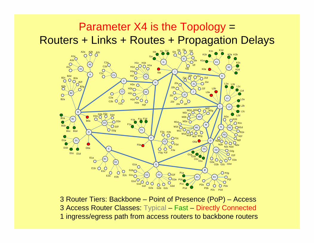
Parameter X4 is the Topology = Routers + Links + Routes + Propagation Delays

A

C

D

E

G

F

J

K

M

P

B

L

N

O

A1

A1b

A1c

A1a

A2b A2cA2a

C1

C1b

C1c

C1a

C2

C2bC2c

C2a

H2b

H2c

H2a

H1

H1bH1cH1a

E1

E1bE1c

E1a

E2bE2cE2a

H1d

H1e

H1f

H2fH2e

H2d

G1b

G1c

G1a

G1eG1d

G2b G2cG2a

G2e

G2dG1f

G2fP1 P2

P1a

P1b

P1c

P1dP2a

P2bP2c P2d

P2e

P2f

P2g

K1

K2K0a

K1a

K1bK1c K1d

K2a K2b

K2c

K2d

L2

L1

L1a L1bL1c

L1d

L2a

L2b

L2c

L2d

L0aL0b

J1

J2

J1aJ1b J1c

J1d

J1e

J1f

J2a

J2b

J2c

J2dJ2e J2f

N1aN1b

N1c

N1d

N1e

N1fN2

N2aN2b

N2c N2dN2e

N2f

M2b

M2cM2d M2e

M2f

M2

M2g

M2aM1a

M1M1b

M1cM1dM1e M1f M1g

O0a

O1aO1b

O1cO1c

O1

O2a

O2

O2b O2c O2d

O2e

O2f

O2g

I2

I2a

I1

II0a

I1a

I1b I1c I1d

I2gI2f

I2e

I2dI2cI2b

F2

F2aF1

F1a

F1b F1c F1d

F2g F2f

F2d

F2c

F2b

F0a

F2e

D2

D2a

D1D1a

D1b

D1c D1d

D2gD2f

D2dD2cD2b

D2e

D0a

B0aB1B1a

B1b

B1c B1d

B2

B2a

B2b

B2cB2d

B2eB2f

B2g

H

G1 G2

E2

H2

A2

N1

3 Router Tiers: Backbone – Point of Presence (PoP) – Access3 Access Router Classes: Typical – Fast – Directly Connected1 ingress/egress path from access routers to backbone routers

Link Characteristics – Propagation Delay and Cost Metric

A

C

D

E

G

F

J

K

M

P

B

L

N

O

A1

A1b

A1c

A1a

A2b A2cA2a

C1

C1b

C1c

C1a

C2

C2bC2c

C2a

H2b

H2c

H2a

H1

H1bH1cH1a

E1

E1bE1c

E1a

E2bE2cE2a

H1d

H1e

H1f

H2fH2e

H2d

G1b

G1c

G1a

G1eG1d

G2b G2cG2a

G2e

G2dG1f

G2fP1 P2

P1a

P1b

P1c

P1dP2a

P2bP2c P2d

P2e

P2f

P2g

K1

K2K0a

K1a

K1bK1c K1d

K2a K2b

K2c

K2d

L2

L1

L1a L1bL1c

L1d

L2a

L2b

L2c

L2d

L0aL0b

J1

J2

J1aJ1b J1c

J1d

J1e

J1f

J2a

J2b

J2c

J2dJ2e J2f

N1aN1b

N1c

N1d

N1eN1f

N2

N2aN2b

N2c N2dN2e

N2f

M2b

M2cM2d M2e

M2f

M2

M2g

M2aM1a

M1M1bM1c

M1dM1e M1f M1g

O0a

O1aO1b

O1cO1c

O1

O2a

O2

O2b O2c O2d

O2e

O2f

O2g

I2

I2a

I1

II0a

I1a

I1b I1c I1d

I2gI2f

I2e

I2dI2cI2b

F2

F2aF1

F1a

F1b F1c F1d

F2g F2f

F2d

F2c

F2b

F0a

F2e

D2

D2a

D1D1a

D1b

D1c D1d

D2gD2f

D2dD2cD2b

D2e

D0a

B0aB1B1a

B1b

B1c B1d

B2

B2a

B2b

B2cB2d

B2eB2f

B2g

H

G1 G2

E2

H2

A2

N1

• Packets incur propagation delaywhen transiting a link

• Cost metric used to compute routesfrom source backbone router to destination backbone router

Link # Link Endpoints Delay (ms) Cost Metric1 A‐B 21 502 B‐C 25 103 B‐D 8 504 B‐L 75 2235 C‐H 12 1006 D‐E 10 107 D‐F 33 1088 E‐G 33 1009 F‐G 7 1010 F‐H 12 5011 F‐I 22 5512 G‐O 23 10413 G‐P 19 11014 I‐H 14 1015 I‐J 8 5016 I‐K 22 14717 J‐L 20 6018 K‐L 7 5019 L‐M 12 5020 L‐N 6 3921 L‐O 14 1022 M‐O 6 1023 N‐O 8 1024 O‐P 14 10

Dijkstra’s SPF Backbone Routes Computed from Cost Metrics

A

C

D

E

G

F

J

K

M

P

B

L

N

O

A1

A1b

A1c

A1a

A2b A2cA2a

C1

C1b

C1c

C1a

C2

C2bC2c

C2a

H2b

H2c

H2a

H1

H1bH1cH1a

E1

E1bE1c

E1a

E2bE2cE2a

H1d

H1e

H1f

H2fH2e

H2d

G1b

G1c

G1a

G1eG1d

G2b G2cG2a

G2e

G2dG1f

G2fP1 P2

P1a

P1b

P1c

P1dP2a

P2bP2c P2d

P2e

P2f

P2g

K1

K2K0a

K1a

K1bK1c K1d

K2a K2b

K2c

K2d

L2

L1

L1a L1bL1c

L1d

L2a

L2b

L2c

L2d

L0aL0b

J1

J2

J1aJ1b J1c

J1d

J1e

J1f

J2a

J2b

J2c

J2dJ2e J2f

N1aN1b

N1c

N1d

N1eN1f

N2

N2aN2b

N2c N2dN2e

N2f

M2b

M2cM2d M2e

M2f

M2

M2g

M2aM1a

M1M1bM1c

M1dM1e M1f M1g

O0a

O1aO1b

O1cO1c

O1

O2a

O2

O2b O2c O2d

O2e

O2f

O2g

I2

I2a

I1

II0a

I1a

I1b I1c I1d

I2gI2f

I2e

I2dI2cI2b

F2

F2aF1

F1a

F1b F1c F1d

F2g F2f

F2d

F2c

F2b

F0a

F2e

D2

D2a

D1D1a

D1b

D1c D1d

D2gD2f

D2dD2cD2b

D2e

D0a

B0aB1B1a

B1b

B1c B1d

B2

B2a

B2b

B2cB2d

B2eB2f

B2g

H

G1 G2

E2

H2

A2

N1

PATHS FOR NODE A PATHS FOR NODE B PATHS FOR NODE C PATHS FOR NODE DA:B @ A‐>B $ 50 B:A @ B‐>A $ 50 C:A @ C‐>B‐>A $ 60 D:A @ D‐>B‐>A $ 100A:C @ A‐>B‐>C $ 60 B:C @ B‐>C $ 10 C:B @ C‐>B $ 10 D:B @ D‐>B $ 50A:D @ A‐>B‐>D $ 100 B:D @ B‐>D $ 50 C:D @ C‐>B‐>D $ 60 D:C @ D‐>B‐>C $ 60A:E @ A‐>B‐>D‐>E $ 110 B:E @ B‐>D‐>E $ 60 C:E @ C‐>B‐>D‐>E $ 70 D:E @ D‐>E $ 10A:F @ A‐>B‐>D‐>F $ 208 B:F @ B‐>D‐>F $ 158 C:F @ C‐>H‐>F $ 150 D:F @ D‐>F $ 108A:G @ A‐>B‐>D‐>E‐>G $ 210 B:G @ B‐>D‐>E‐>G $ 160 C:G @ C‐>H‐>F‐>G $ 160 D:G @ D‐>E‐>G $ 110A:H @ A‐>B‐>C‐>H $ 160 B:H @ B‐>C‐>H $ 110 C:H @ C‐>H $ 100 D:H @ D‐>F‐>H $ 158A:I @ A ‐> B ‐> C ‐> H ‐> I $ 170 B:I @ B ‐> C ‐> H ‐> I $ 120 C:I @ C ‐> H ‐> I $ 110 D:I @ D ‐> F ‐> I $ 163A:J @ A‐>B $220 B:J @ B‐>C $170 C:J @ C‐>H $160 D:J @ D‐>F $213A:K @ A‐>B‐>C‐>H‐>I‐>K $ 317 B:K @ B‐>C‐>H‐>I‐>K $ 267 C:K @ C‐>H‐>I‐>K $ 257 D:K @ D‐>F‐>I‐>K $ 310A:L @ A‐>B‐>L $ 273 B:L @ B‐>L $223 C:L @ C‐>H $220 D:L @ D‐>E‐>G‐>O‐>N‐>L $ 263A:M @ A‐>B‐>L‐>M $ 323 B:M @ B‐>L‐>M $ 273 C:M @ C‐>H‐>I‐>J‐>L‐>M $ 270 D:M @ D‐>E‐>G‐>O‐>M $ 224A:N @ A‐>B‐>L‐>N $ 312 B:N @ B‐>L‐>N $ 262 C:N @ C‐>H‐>I‐>J‐>L‐>N $ 259 D:N @ D‐>E‐>G‐>O‐>N $ 224A:O @ A‐>B‐>D‐>E‐>G‐>O $ 314 B:O @ B‐>D‐>E‐>G‐>O $ 264 C:O @ C‐>H‐>F‐>G‐>O $ 264 D:O @ D‐>E‐>G‐>O $ 214A:P @ A‐>B‐>D‐>E‐>G‐>P $ 320 B:P @ B‐>D‐>E‐>G‐>P $ 270 C:P @ C‐>H‐>F‐>G‐>P $ 270 D:P @ D‐>E‐>G‐>P $ 220

PATHS FOR NODE E PATHS FOR NODE F PATHS FOR NODE G PATHS FOR NODE HE:A @ E‐>D‐>B‐>A $ 110 F:A @ F‐>D‐>B‐>A $ 208 G:A @ G‐>E‐>D‐>B‐>A $ 210 H:A @ H‐>C‐>B‐>A $ 160E:B @ E‐>D‐>B $ 60 F:B @ F‐>D‐>B $ 158 G:B @ G‐>E‐>D‐>B $ 160 H:B @ H‐>C‐>B $ 110E:C @ E‐>D‐>B‐>C $ 70 F:C @ F‐>H‐>C $ 150 G:C @ G‐>F‐>H‐>C $ 160 H:C @ H‐>C $ 100E:D @ E‐>D $ 10 F:D @ F‐>D $ 108 G:D @ G‐>E‐>D $ 110 H:D @ H‐>F‐>D $ 158E:F @ E‐>G‐>F $ 110 F:E @ F‐>G‐>E $ 110 G:E @ G‐>E $ 100 H:E @ H‐>F‐>G‐>E $ 160E:G @ E‐>G $ 100 F:G @ F‐>G $ 10 G:F @ G‐>F $ 10 H:F @ H‐>F $ 50E:H @ E‐>G‐>F‐>H $ 160 F:H @ F‐>H $ 50 G:H @ G‐>F‐>H $ 60 H:G @ H‐>F‐>G $ 60E:I @ E ‐> G ‐> F ‐> I $ 165 F:I @ F ‐> I $ 55 G:I @ G ‐> F ‐> I $ 65 H:I @ H ‐> I $ 10E:J @ E‐>G $215 F:J @ F ‐> I ‐> J $ 105 G:J @ G‐>F $115 H:J @ H‐>I ‐> J $60E:K @ E‐>G‐>O‐>N‐>L‐>K $ 303 F:K @ F‐>I ‐> K $ 202 G:K @ G‐>O‐>N‐>L‐>K $ 203 H:K @ H‐> $157E:L @ E‐>G‐>O‐>N‐>L $ 253 F:L @ F‐>G‐>O‐>N‐>L $ 163 G:L @ G‐>O‐>N‐>L $ 153 H:L @ H‐>I ‐> L$ 120E:M @ E‐>G‐>O‐>M $ 214 F:M @ F‐>G‐>O‐>M $ 124 G:M @ G‐>O‐>M $ 114 H:M @ H‐>I‐>J‐>L‐>M $ 170E:N @ E‐>G‐>O‐>N $ 214 F:N @ F‐>G‐>O‐>N $ 124 G:N @ G‐>O‐>N $ 114 H:N @ H‐>I‐>J‐>L‐>N $ 159E:O @ E‐>G‐>O $ 204 F:O @ F‐>G‐>O $ 114 G:O @ G‐>O $ 104 H:O @ H‐>F‐>G‐>O $ 164E:P @ E‐>G‐>P $ 210 F:P @ F‐>G‐>P $ 120 G:P @ G‐>P $ 110 H:P @ H‐>F‐>G‐>P $ 170

9.533.63240

Avg. Source-Receiver Path LengthAvg. Backbone Path Length# Backbone Paths

9.533.63240

Avg. Source-Receiver Path LengthAvg. Backbone Path Length# Backbone Paths

Sample Backbone Paths for Routers A Through H

Parameter x2 scales all propagation delaysLink # Link Endpoints Delay (ms) x2 = 2 x2 = 0.5 1 A‐B 21 42 10.52 B‐C 25 50 12.53 B‐D 8 16 44 B‐L 75 150 37.55 C‐H 12 24 66 D‐E 10 20 57 D‐F 33 66 16.58 E‐G 33 66 16.59 F‐G 7 14 3.510 F‐H 12 24 611 F‐I 22 44 1112 G‐O 23 46 11.513 G‐P 19 38 9.514 I‐H 14 28 715 I‐J 8 16 416 I‐K 22 44 1117 J‐L 20 40 1018 K‐L 7 14 3.519 L‐M 12 24 620 L‐N 6 12 321 L‐O 14 28 722 M‐O 6 12 323 N‐O 8 16 424 O‐P 14 28 7

Engineering Relationship Among Router Speeds(MesoNet simplification – only routers have speeds)

Speed RelationshipsRouter Class SpeedBackbone r1 x BBspeedupPoP r1/r2Access r1/r2/r3Fast Access r1/r2/r3 x BfastDirectly Connected Access r1/r2/r3 x Bdirect

Parameter Valuer1 x1r2 4r3 10BBspeedup 2Bdirect 10Bfast 2

Sample Parameters Values

Router Class Speed x1 = 800 x1 = 1600Backbone r1 x BBspeedup 1600 3200PoP r1/r2 400 800Access r1/r2/r3 40 80Fast Access r1/r2/r3 x Bfast 80 160Directly Connected Access r1/r2/r3 x Bdirect 400 800

Parameter x1 scales all router speedsGiven a fixed r2, r3, BBspeedup, Bdirect and Bfast,

Domain View of Network Speed(MesoNet simplification – packets have no size)

^default maximum transfer unit size for the Internet is 1500 bytes

Assuming speeds dimensioned in packets per millisecondsand packets sized at 1500^ 8-bit bytes:

Router Class x1 = 800 Speed (Gbps) x1 = 1600 Speed (Gbps)Backbone 1600 19.2 3200 38.4PoP 400 4.8 800 9.6Access 40 0.48 80 0.96Fast Access 80 0.96 160 1.92Directly Connected Access 400 4.8 800 9.6

Buffer Size Determination

CRTT ×

nCRTT )( ×

Choice of 4 Buffer Provisioning Algorithmsrecommended practice

suggested by researchers from Stanford

2)))(()(( nCRTTCRTT ×+× interpolation

Buffers =

directly set

Buffers =

Buffers =

Buffers = <integer value>

RTT = average round-trip propagation delay of the topologyC = capacity of a given router type – determined by network speed settingsn = expected number of flows transiting the router

Qfactor = buffer size scaling factor

BufferSize = Buffers x Qfactor

For selected algorithm, x3 = Qfactor scales buffer size For specified Qfactor, x3 = algorithm determines buffer size

Sources & Receivers

Approximate Number of Sources & Receivers

baseSources = target^ # sources under each access routerU = scaling factor for target # sources

# sources = O(baseSources x U x # access routers) # receivers = O(baseSources x U x # access routers x 4)

O(204,000)O(51,000)3

O(68,000)O(17,000)1

# receivers# sourcesUbaseSources = 100 # access routers = 170

^# sources and receivers becomes known exactly only when taking into account the distribution of sources and receivers under various access router types

Setting x6 (= U) scales the number of sources and receivers in the network

Access Router Classes & Source Distribution

1 – probNs - probNsf

probNsf

probNs

Probability Source Under

Directly connected access routersD-class

Access routers with fast speedF-class

Access routers with typical speedN-class

Access Router Classes

Setting x7 = (probNs, probNsf) scales the distribution of sources and adjusts the number of sources in the topology

Setting x8 = (probNr, probNrf) performs a similar function on receivers

Target # sources under 3 access routers: 1 in each class) = 3 x baseSources x U# sources under each N-class router = 3 x baseSources x U x probNs

# sources under each F-class router = 3 x baseSources x U x probNsf

# sources under each D-class router = 3 x baseSources x U x (1 - probNs - probNsf)

6.2

62.2

31.6

% sources

2,160

21,600

10,980

# sources

8

40

122

# routers

270D-class

540F-class

90N-class

sources/routerrouter class

Given U = 3, baseSources = 100, probNs = 0.1, probNsf = 0.6

Total Sources in Network

34,740

Source/Receiver Distributions Influence Traffic Patterns

0.86.2D-class

3.962.2F-class

95.331.6N-class

% receivers% sourcesrouter class

Given U = 3, baseSources = 100, probNs = 0.1, probNsf = 0.6, probNr = 0.8, probNrf = 0.1

30.1NN flows

60.5FN flows

2.4FF flows

6.1DN flows

0.74DF flows

0.05DD flows

% flowsFlow class

FF, FN, DN and DF flows represent Web-centric traffic and NN flows represent P2P-like traffic

DD flows represent traffic exchange with large data repositories

Source & Receiver Interface Speeds

96080Hfast

968Hbase

MbpsppmsInterface Speeds

Assuming packet size is 1500 8-bit bytes:

Model permits two interface speeds

x5 specifies the probability that a source/receiver has an Hfast interface

(1- x5) gives the probability that a source/receiver has an Hbase interface

Example

User Behavior

Source Behavior^

^Note: this simplified diagram omits a flow connection phase that occurs before sending and also the potential for the connection phase to fail – after which source enters Thinking

x11 specifies average Think Time x12 specifies probability source is reactive

Think Time Expired

Select Receiver &File Size (Pareto Distribution)

Finished

Select Think Time(Exponential Distribution)


Too Long(reactive sources only)

Too Slow (reactive sources only)


Select Receiver &File Size (Pareto Distribution)


File Size Selection

x9 specifies on

shape of Pareto distribution

average size (packets)on

Size of Web Objects

moviesMx

software downloadsSx

documentsFx

Larger File Size Multipliers

moviesMp

software downloadsSp

documentsFp

Larger File Probabilities

Probability of Web Object (1 – Fp – Sp – Mp)

Given a fixed Given fixed Fx, Sx, Mxx10 specifies (Fp, Sp, Mp)

Characterize Web Objects ( on, )

Characterize Larger Files [(Fx, Fp), (Sx, Sp), (Mx, Mp)]

Specifying Intense Spatiotemporal Traffic

x13 specifies (Jon, Joff)

fraction of simulated time after which jumbo file transfers endJoff

fraction of simulated time after which jumbo file transfers beginJon

size multiplier for jumbo filesJx

Jumbo File Characteristics

During selected time periods, DD flows can transfer jumbo files

Given a fixed Jx

Characterize Jumbo Files (Jx, Jon, Joff)

Specifying Long-Lived Flows

x14 specifies (n, LLon, SourceType, SourceLocation, ReceiverLocation)

Behavior of each long-lived flow is monitored in detail

access router under which each long-lived receiver is locatedReceiverLocation[n]

access router under which each long-lived source is locatedSourceLocation[n]

congestion control algorithm used by each long-lived flowSourceType[n]

fraction of simulated time after which each long-lived flow startsLLon[n]

number of long-lived flowsn

Characteristics of Long-Lived Flows

BIC7

HTCP6

FAST5

Scalable TCP4

CTCP3

HSTCP2

TCP1

select from probability distribution (see x15)0

Source TypeID

Protocols

Assignment of Congestion Control AlgorithmProbabilistically assign each source (except for long-lived flows) a congestion control algorithm

prBICTCPBIC

prHTCPHTCP

prFASTFAST

prSCALABLEScalable TCP

prCTCPCTCP

prHSTCPHSTCP

prTCPTCP

Probability

Congestion Control

Algorithm

x15 specifies (prTCP, prHSTCP, prCTCP, prSCALABLE, prFAST, prHTCP, prBICTCP)

Initial Congestion Window & Slow Start ThresholdCongestion window (cwnd) determines how many packets may be sent by a source in one RTT

At Initial Slow Start Threshold (sst) cwnd increase switches from exponential to linear

0

20

40

60

80

100

120

140

160

0 20 40 60 80 100

Time

CW

ND

Initial cwnd

Initial sst

exponentialincrease

linearincrease

0

20

40

60

80

100

120

140

160

0 20 40 60 80 100

Time

CW

ND

Initial cwnd

Initial sst

0

20

40

60

80

100

120

140

160

0 20 40 60 80 100

Time

CW

ND

Initial cwnd

Initial sst

0

20

40

60

80

100

120

140

160

0 20 40 60 80 100

Time

CW

ND

Initial cwnd

Initial sst

0

20

40

60

80

100

120

140

160

0 20 40 60 80 100

Time

CW

ND

Initial cwnd

Initial sst

0

20

40

60

80

100

120

140

160

0 20 40 60 80 100

Time

CW

ND

0

20

40

60

80

100

120

140

160

0 20 40 60 80 100

Time

CW

ND

Initial cwnd

Initial sst

exponentialincrease

linearincrease

Initial cwnd determines how many packets may be sent prior to first acknowledgment

x16 specifies initial cwnd x17 specifies initial sst

Simulation & Measurement Control

Measurement Interval Size & Simulation DurationMeasurements taken as time series sampled periodically: every measurement interval

simulation durationM x MI

number of measurement intervalsMI

measurement interval sizeM

Controlling Measurement & Simulation Length

3000 3500 4000 4500 5000 5500 6000 6500 7000 75000

1000

2000

3000

4000

5000

6000

7000

8000

9000Evolution of Flows Condition 5 - TCP

Time

Act

ive F

low

s

Sending Flows

Normal Congestion Control

Connecting Flows

Flows in Initial Slow Start

3000 3500 4000 4500 5000 5500 6000 6500 7000 75000

1000

2000

3000

4000

5000

6000

7000

8000

9000Evolution of Flows Condition 5 - TCP

Time

Act

ive F

low

s

Sending Flows

Normal Congestion Control

Connecting Flows

Flows in Initial Slow Start

x18 specifies M x19 specifies MI

Source Startup PatternSources enter the sending state at simulation startup according to a specified pattern

probability a source starts sending after random time: mean think timeprREST

probability a source starts sending after random time: mean 66% x think timeprONthird

probability a source starts sending after random time: mean 33% x think time prONsecond

probability a source starts in the sending stateprON

Initial Think Times for Sources

x20 specifies (prON, prONsecond, prONthird)

prREST = (1 – prON – prONsecond – prONthird)

0

1000

2000

3000

4000

5000

6000

0 50 100 150 200 250Time

Send

ing

Flow

s

0.50prREST

0.17prONthird

0.08prONsecond

0.25prON

Two Sample Experiments

BIC, CTCP, FAST, FAST-AT, HSTCP,

HTCP, Scalable


HTCP, Scalable

Alternate Congestion-Control Algorithms

60 min. – 96-98% Web objects; 2-4% document transfers; smaller number of service-pack and movie downloads

30:70 & 70:30

232/2

1x10-4 to 1x10-2

19.2 & 38.417,455 & 26,085

Sec. 8 High SST


Scenario

30:70 & 70:30

Ratio (%) of Sources using Alternate Congestion-Control to Standard TCP Congestion-Control

232/2Initial Slow-Start Threshold

2x10-9 to 2x10-2Packet Loss Rate

192 & 384Backbone Speed (Gbps)174,600 & 261,792Network Size (sources)

Sec. 9 High SSTCharacteristic


HTCP, Scalable


HTCP, Scalable

Alternate Congestion-Control Algorithms


30:70 & 70:30

232/2

1x10-4 to 1x10-2

19.2 & 38.417,455 & 26,085

Sec. 8 High SST


Scenario

30:70 & 70:30

Ratio (%) of Sources using Alternate Congestion-Control to Standard TCP Congestion-Control

232/2Initial Slow-Start Threshold

2x10-9 to 2x10-2Packet Loss Rate

192 & 384Backbone Speed (Gbps)174,600 & 261,792Network Size (sources)

Sec. 9 High SSTCharacteristic

Joint work with Jim Filliben, Dong Yeon Cho and Edward Schwartz

7 Congestion Control Algorithms x 32 Conditions

Factor-> x1 x2 x3 x4 x5 x6 x7 x8 x9Condition -- -- -- -- -- -- -- -- --

1 8000 1 0.5 5000 100 0.04/0.004/0.0004 0.7 0.7 32 16000 1 0.5 5000 100 0.04/0.004/0.0004 0.3 0.3 23 8000 2 0.5 5000 100 0.02/0.002/0.0002 0.7 0.3 24 16000 2 0.5 5000 100 0.02/0.002/0.0002 0.3 0.7 35 8000 1 1 5000 100 0.02/0.002/0.0002 0.3 0.7 26 16000 1 1 5000 100 0.02/0.002/0.0002 0.7 0.3 37 8000 2 1 5000 100 0.04/0.004/0.0004 0.3 0.3 38 16000 2 1 5000 100 0.04/0.004/0.0004 0.7 0.7 29 8000 1 0.5 7500 100 0.02/0.002/0.0002 0.3 0.3 3

10 16000 1 0.5 7500 100 0.02/0.002/0.0002 0.7 0.7 211 8000 2 0.5 7500 100 0.04/0.004/0.0004 0.3 0.7 212 16000 2 0.5 7500 100 0.04/0.004/0.0004 0.7 0.3 313 8000 1 1 7500 100 0.04/0.004/0.0004 0.7 0.3 214 16000 1 1 7500 100 0.04/0.004/0.0004 0.3 0.7 315 8000 2 1 7500 100 0.02/0.002/0.0002 0.7 0.7 316 16000 2 1 7500 100 0.02/0.002/0.0002 0.3 0.3 217 8000 1 0.5 5000 150 0.02/0.002/0.0002 0.3 0.3 218 16000 1 0.5 5000 150 0.02/0.002/0.0002 0.7 0.7 319 8000 2 0.5 5000 150 0.04/0.004/0.0004 0.3 0.7 320 16000 2 0.5 5000 150 0.04/0.004/0.0004 0.7 0.3 221 8000 1 1 5000 150 0.04/0.004/0.0004 0.7 0.3 322 16000 1 1 5000 150 0.04/0.004/0.0004 0.3 0.7 223 8000 2 1 5000 150 0.02/0.002/0.0002 0.7 0.7 224 16000 2 1 5000 150 0.02/0.002/0.0002 0.3 0.3 325 8000 1 0.5 7500 150 0.04/0.004/0.0004 0.7 1 226 16000 1 0.5 7500 150 0.04/0.004/0.0004 0.3 0.3 327 8000 2 0.5 7500 150 0.02/0.002/0.0002 0.7 0.3 328 16000 2 0.5 7500 150 0.02/0.002/0.0002 0.3 0.7 229 8000 1 1 7500 150 0.02/0.002/0.0002 0.3 0.7 330 16000 1 1 7500 150 0.02/0.002/0.0002 0.7 0.3 231 8000 2 1 7500 150 0.04/0.004/0.0004 0.3 0.3 232 16000 2 1 7500 150 0.04/0.004/0.0004 0.7 0.7 3

29-4 Orthogonal Fractional Factorial Design

(7 x 32 =) 224 Runs for Small, Slow Network and (7 x 32 =) 224 Runs for Large, Fast Network

Note: factor designators x1 to x9 not the same as used in this talk

MesoNet Tractable?Large, Fast Network with High

Initial Slow-Start ThresholdSmall, Slow Network with High

Initial Slow-Start Threshold

2,568,480,12217,390,7817,258,056

11,466,429

Flows Completed

764,739,915,9785,048,119,1662,138,998,7643,414,017,482

Data Packets Sent

7,470,633,040,19926,055,028,851Total all Runs50,932,067,100175,947,632Max. Per Condition21,069,357,40972,944,797Min. Per Condition33,351,040,358116,317,093Avg. Per Condition

Data Packets SentFlows CompletedStatistic

Large, Fast Network with High Initial Slow-Start Threshold

Small, Slow Network with High Initial Slow-Start Threshold

2,568,480,12217,390,7817,258,056

11,466,429

Flows Completed

764,739,915,9785,048,119,1662,138,998,7643,414,017,482

Data Packets Sent

7,470,633,040,19926,055,028,851Total all Runs50,932,067,100175,947,632Max. Per Condition21,069,357,40972,944,797Min. Per Condition33,351,040,358116,317,093Avg. Per Condition

Data Packets SentFlows CompletedStatistic

739.0443.97Max. CPU hours(one run)

2,392.41196.56Avg. Memory Usage (Mbytes)

203.0412.58Min. CPU hours(one run)

421.2326.15Avg. CPU hours(per run)

94,355.285,857.18CPU hours (224 Runs)

Large, Fast Network with High Initial Slow-

Start Threshold

Small, Slow Network with High Initial Slow-

Start Threshold

739.0443.97Max. CPU hours(one run)

2,392.41196.56Avg. Memory Usage (Mbytes)

203.0412.58Min. CPU hours(one run)

421.2326.15Avg. CPU hours(per run)

94,355.285,857.18CPU hours (224 Runs)

Large, Fast Network with High Initial Slow-

Start Threshold

Small, Slow Network with High Initial Slow-

Start Threshold

48 processors available to run simulations

competed in 1 week competed in 3 months35 weeks of CPU time 131 months of CPU time

Future Work

• Conduct 20-factor sensitivity analysis of MesoNet [data analysis underway]

• Use MesoNet to compare proposed Internet congestion control algorithms [report drafted]

• Develop a reduced scale simulation model for cloud computing IaaS (infrastructure-as-a-service) [studying literature, code and deployments]

• Conduct sensitivity analysis of IaaS model• Compare proposed IaaS resource

allocation algorithms [studying literature and code]

JOINT WORK BETWEEN CxS and CNS Programs

Joint work with Chris Dabrowski, Jim Filliben and Peter Mell

Backup Slides

Dijkstra’s SPF Backbone Routes Computed from Cost Metrics (2 of 2)

A

C

D

E

G

F

J

K

M

P

B

L

N

O

A1

A1b

A1c

A1a

A2b A2cA2a

C1

C1b

C1c

C1a

C2

C2bC2c

C2a

H2b

H2c

H2a

H1

H1bH1cH1a

E1

E1bE1c

E1a

E2bE2cE2a

H1d

H1e

H1f

H2fH2e

H2d

G1b

G1c

G1a

G1eG1d

G2b G2cG2a

G2e

G2dG1f

G2fP1 P2

P1a

P1b

P1c

P1dP2a

P2bP2c P2d

P2e

P2f

P2g

K1

K2K0a

K1a

K1bK1c K1d

K2a K2b

K2c

K2d

L2

L1

L1a L1bL1c

L1d

L2a

L2b

L2c

L2d

L0aL0b

J1

J2

J1aJ1b J1c

J1d

J1e

J1f

J2a

J2b

J2c

J2dJ2e J2f

N1aN1b

N1c

N1d

N1eN1f

N2

N2aN2b

N2c N2dN2e

N2f

M2b

M2cM2d M2e

M2f

M2

M2g

M2aM1a

M1M1bM1c

M1dM1e M1f M1g

O0a

O1aO1b

O1cO1c

O1

O2a

O2

O2b O2c O2d

O2e

O2f

O2g

I2

I2a

I1

II0a

I1a

I1b I1c I1d

I2gI2f

I2e

I2dI2cI2b

F2

F2aF1

F1a

F1b F1c F1d

F2g F2f

F2d

F2c

F2b

F0a

F2e

D2

D2a

D1D1a

D1b

D1c D1d

D2gD2f

D2dD2cD2b

D2e

D0a

B0aB1B1a

B1b

B1c B1d

B2

B2a

B2b

B2cB2d

B2eB2f

B2g

H

G1 G2

E2

H2

A2

N1

PATHS FOR NODE I PATHS FOR NODE J PATHS FOR NODE K PATHS FOR NODE LI : A @ I ‐> H ‐> C ‐> B ‐> A $ 170 J : A @ J ‐> I ‐> H ‐> C ‐> B ‐> A $ 220 K:A @ K‐>I‐>H‐>C‐>B‐>A $ 317 L:A @ L‐>B‐>A $ 273I : B @ I ‐> H ‐> C ‐> B $ 120 J : B @ J ‐> I ‐> H ‐> C ‐> B $ 170 K:B @ K‐>I‐>H‐>C‐>B $ 267 L:B @ L‐>B $223I : C @ I ‐> H ‐> C $ 110 J : C @ J ‐> I ‐> H ‐> C $ 160 K:C @ K‐>I‐>H‐>C $ 257 L:C @ L‐>J‐‐> H ‐> C $ 220I : D @ I ‐> F ‐> D $ 163 J : D @ J ‐> I ‐> F ‐> D $ 213 K:D @ K‐>I‐>F‐>D $ 310 L:D @ L‐>N‐>O‐>G‐>E‐>D $ 263I : E @ I ‐> F ‐> G ‐> E $ 165 J : E @ J ‐> I ‐> F ‐> G ‐> E $ 215 K:E @ K‐>L‐>N‐>O‐>G‐>E $ 303 L:E @ L‐>N‐>O‐>G‐>E $ 253I : F @ I ‐> F $ 55 J : F @ J ‐> I ‐> F $ 105 K:F @ K‐>I ‐> F $ 202 L:F @ L‐>N‐>O‐>G‐>F $ 163I : G @ I ‐> F ‐> G $ 65 J : G @ J ‐> I ‐> F ‐> G $ 115 K:G @ K‐>L‐>N‐>O‐>G $ 203 L:G @ L‐>N‐>O‐>G $ 153I : H @ I ‐> H $ 10 J : H @ J ‐> I ‐> H $ 60 K:H @ K‐>I $157 L:H @ L‐>J ‐> H $ 120I : J @ I ‐> J $ 50 J : I @ J ‐> I $ 50 K:I @ K ‐> I $ 147 L:I @ L ‐> J ‐> I $ 110I : K @ I ‐> K $ 147 J : K @ J ‐> L ‐> K $ 110 K:J @ K‐>L $110 L:J @ L ‐> J $ 60I : L @ I ‐> J ‐> L $ 110 J : L @ J ‐> L $ 60 K:L @ K‐>L $50 L:K @ L‐>K $50I : M @ I ‐> J ‐> L ‐> M $ 160 J : M @ J ‐> L ‐> M $ 110 K:M @ K‐>L‐>M $ 100 L:M @ L‐>M $ 50I : N @ I ‐> J ‐> L ‐> N $ 149 J : N @ J ‐> L ‐> N $ 99 K:N @ K‐>L‐>N $ 89 L:N @ L‐>N $ 39I : O @ I ‐> J ‐> L ‐> N ‐> O $ 159 J : O @ J ‐> L ‐> N ‐> O $ 109 K:O @ K‐>L‐>N‐>O $ 99 L:O @ L‐>N‐>O $ 49I : P @ I ‐> J ‐> L ‐> N ‐> O ‐> P $ 169 J : P @ J ‐> L ‐> N ‐> O ‐> P $ 119 K:P @ K‐>L‐>N‐>O‐>P $ 109 L:P @ L‐>N‐>O‐>P $ 59

PATHS FOR NODE M PATHS FOR NODE N PATHS FOR NODE O PATHS FOR NODE PM:A @ M‐>L‐>B‐>A $ 323 N:A @ N‐>L‐>B‐>A $ 312 O:A @ O‐>G‐>E‐>D‐>B‐>A $ 314 P:A @ P‐>G‐>E‐>D‐>B‐>A $ 320M:B @ M‐>L‐>B $ 273 N:B @ N‐>L‐>B $ 262 O:B @ O‐>G‐>E‐>D‐>B $ 264 P:B @ P‐>G‐>E‐>D‐>B $ 270M:C @ M‐>L‐>J‐>I‐>H‐>C $ 270 N:C @ N‐>L‐>J‐>I‐>H‐>C $ 259 O:C @ O‐>G‐>F‐>H‐>C $ 264 P:C @ P‐>G‐>F‐>H‐>C $ 270M:D @ M‐>O‐>G‐>E‐>D $ 224 N:D @ N‐>O‐>G‐>E‐>D $ 224 O:D @ O‐>G‐>E‐>D $ 214 P:D @ P‐>G‐>E‐>D $ 220M:E @ M‐>O‐>G‐>E $ 214 N:E @ N‐>O‐>G‐>E $ 214 O:E @ O‐>G‐>E $ 204 P:E @ P‐>G‐>E $ 210M:F @ M‐>O‐>G‐>F $ 124 N:F @ N‐>O‐>G‐>F $ 124 O:F @ O‐>G‐>F $ 114 P:F @ P‐>G‐>F $ 120M:G @ M‐>O‐>G $ 114 N:G @ N‐>O‐>G $ 114 O:G @ O‐>G $ 104 P:G @ P‐>G $ 110M:H @ M‐>L‐>J‐>I‐>H $ 170 N:H @ N‐>L‐>J‐>I‐>H $ 159 O:H @ O‐>G‐>F‐>H $ 164 P:H @ P‐>G‐>F‐>H $ 170M:I @ M ‐> L ‐> J ‐> I $ 160 N:I @ N ‐> L ‐> J ‐> I $ 149 O:I @ O ‐> N ‐> L ‐> J ‐> I $ 159 P:I @ P ‐> O ‐> N ‐> L ‐> J ‐> I $ 169M:J @ M‐>L‐>J $ 110 N:J @ N‐>L $99 O:J @ O‐>N‐>L‐>J $ 109 P:J @ P‐>O‐>N‐>L‐>J $ 119M:K @ M‐>L‐>K $ 100 N:K @ N‐>L‐>K $ 89 O:K @ O‐>N‐>L‐>K $ 99 P:K @ P‐>O‐>N‐>L‐>K $ 109M:L @ M‐>L $ 50 N:L @ N‐>L $ 39 O:L @ O‐>N‐>L $ 49 P:L @ P‐>O‐>N‐>L $ 59M:N @ M‐>O‐>N $ 20 N:M @ N‐>O‐>M $ 20 O:M @ O‐>M $ 10 P:M @ P‐>O‐>M $ 20M:O @ M‐>O $ 10 N:O @ N‐>O $ 10 O:N @ O‐>N $ 10 P:N @ P‐>O‐>N $ 20M:P @ M‐>O‐>P $ 20 N:P @ N‐>O‐>P $ 20 O:P @ O‐>P $ 10 P:O @ P‐>O $ 10

Other Sample MesoNetTopologies

Sample Dumbbell Topology from an Empirical Study

Sample Simulated Topology (I) from MesoNet

Sample Simulated Topology (IIc & IId) from MesoNet

IIc – asymmetric routesIId – SPF based on propagation delay

Sample Simulated Topology (ST) from MesoNet

A

B

D

C

F

G

H

I

K

J

E

B0a

F0a

I0a

I1a

Sources B0a1-B0a5

Sources B0a6-B0a10

Sources F0a1-F0a5 Sources F0a6-F0a10

H0a

Sources H0a1-H0a5Sources H0a6-H0a10

Receivers K0a1-K0a5

K0a

Receivers K0a6-K0a10

Receivers I0a1-I0a5 Receivers I0a6-I0a10

Receivers I1a1-I1a5

Receivers I1a6-I1a10Bottleneck Link

SPF based on propagation delays

Documents

How to model a TCP-IP network using only 20 parameters